INFLUENCE OF GNSS CONFIGURATION AND MAP INTERPOLATION METHOD ON INSAR ATMOSPHERIC PHASE ASSESSMENT

Elisabeth Simonetto (1), Frédéric Durand (1), Laurent Morel (1), Yassine El Hamri (1),

Jean-Luc Froger (2), Joëlle Nicolas (1), Stéphane Durand (1), Laurent Polidori (1)

(1) GeF/L2G, ESGT, CNAM, 1 Bd Pythagore, 72000 Le Mans, France, Email: elisabeth.simonetto@cnam.fr (2) LMV, OPGC, Université Blaise pascal, 5 rue Kessler, 63038 Clermont-Ferrand, France, Email:

J.L.Froger@opgc.univ-bpclermont.fr

ABSTRACT

Radar interferometry has proven to be a relevant technique in many application contexts. However, although the development of advanced processing, the interpretation of interferometric measurements is still disturbed by the presence of an atmospheric signal. In this work, we deal with the correction of interferograms using tropospheric delays measured from GNSS stations. We propose some experiments that enhance the influence of different factors in the processing of tropospheric maps. The results show that the interpolation strategy and the GNSS network geometry have a significant impact on the correction. 1. INTRODUCTION

Radar interferometry has proven to be a relevant technique since the last twenty years in many application contexts: geoscience, post-mining, urban survey, landslide, man-made structure monitoring... Nowadays, the largest choice in methods, software, radar data archive or new images, facilitates the use of this technique. However, it will fail in the case of important ground change and its measurements are influenced by the atmosphere crossing (e.g. [1], [2]). In order to estimate the atmospheric signal in InSAR data, several methodologies have been studied by the past using one or several approaches in synergy: standard weather models (e.g. [3], [4]), spectrometer measurements such as MERIS data (e.g. [4], [5]), ground meteorological data (e.g. [6]), adapted filtering (e.g. [7], [8]), advanced InSAR (e.g. [9], [10], [11]), or GNSS (e.g. [12], [13], [14], [15], [16]). In this article, tropospheric corrections are evaluated from GNSS data. The main limitation of this approach is the spatial sampling of the available GNSS stations. One can expect that the GNSS measurement interpolation will have a significant impact on the corrections. In this context, we make comparisons of the tropospheric corrections from GNSS data in terms of the GNSS station number, their spatial distribution and the interpolation method. The test area is the Piton de la Fournaise volcano, La Réunion, France.

2. METHODOLOGY

2.1. Phase modelling in INSAR

The propagation of radar waves in the atmosphere induces significant delays and path deviation. As consequence, an interferogram that is computed between two radar images, named 1 and 2, contains an atmospheric signal relative to the delay written (e.g. [1]):

atmoatmo r∆=∆λπϕ 4 , 1,12,2 atmoatmoatmo rrr −=∆ (1)

In Eq. 1, λ is the radar wavelength. rk,atmok is the path delay of the radar wave propagation in the atmosphere for the data k at the radar image acquisition time:

∫=S

P

z

z

kgatmokk dz

zznr

)(cos)(,

, θ (2)

Where zP and zS are respectively the altitudes of the target and the sensor. θ(z) is the incidence angle in terms of altitude and ng,k(z) is the group refractive index in terms of altitude. Two atmospheric strata are mainly involved in this phenomenon: ionosphere and troposphere:

tropoionoatmo ϕϕϕ ∆+∆=∆

ionoionoiono ,1,2 ϕϕϕ −=∆ (3)

tropotropotropo ,1,2 ϕϕϕ −=∆

where ionok,ϕ and tropok,ϕ are respectively the

ionospheric phase delay and the tropospheric phase delay for image k at target point. The ionospheric phase delay can be expressed in the following way (e.g. [17]):

( ) TECf

PP

iono 210 2

1

1024.1

1

cos

14

×=

θλπϕ (4)

where θP is the incidence angle at target point P, f the

_____________________________________ Proc. ‘Fringe 2015 Workshop’, Frascati, Italy 23–27 March 2015 (ESA SP-731, May 2015)

radar frequency in MHz and TEC is the total electronic content at acquisition time of a radar image. The TEC depends on the geographic location, local time, the season and solar activity. The tropospheric phase delay is written (see e.g. [1]):

( ) ( )∫−

= s

P

z

zP

tropo dzzNPθλ

πϕcos

1046

(5)

where N(z) is the refractive co-index along the wave path for pixel P. Tropospheric refractive index is well expressed in [18]. One can also write:

( ) ( )PSTDPtropo λπϕ 4= (6)

where STD(P) is the Slant Total Delay, that is the total tropospheric delay observed from P-point to the radar sensor. In this work, we only deal with the tropospheric signal. 2.2. GNSS contribution

As in radar imagery, the delay in the propagation of electromagnetic wave due to the troposphere is mandatory in space geodetic techniques such as Global Navigation Satellite Systems (GNSS). This tropospheric delay is mitigated by using a model such as those recommended in the IERS Convention 2010 [19]. These models are usually expressed as followed:

( ) ( ). . . .cos .sinH W G N ESTD ZHD mf el ZWD mf el mf G Az G Az= + + + (7)

The total tropospheric delay observed at the zenith of a GNSS station, i.e. the Zenith Total Delay (ZTD), is divided into the Zenith Hydrostatic Delay (ZHD) and the Zenith Wet Delay (ZWD) which represent about 90% and 10% of the total delay respectively. The hydrostatic and wet delays are mapped down to any elevation angle el using the corresponding hydrostatic and wet functions (mfH , mfW) to provide the Slant Total Delay (STD), i.e. the delay in the direction of the satellite. In these tropospheric models, the ZHD and the mapping functions are assumed to be known a priori (i.e. modelled) while the ZWD are estimated. The computed GPS ZTD can then be used for the InSAR correction. 2.3. Combination

The correction is based on the direct modelling of the atmospheric phase screen (APS) at each radar image acquisition time. APS corresponds to the radar atmospheric phase delay. It is derived from the radar acquisition parameters (satellite locations and velocities, SAR sensor characteristics, acquisition time) and an interpolated map of the GNSS ZTD measurements. Besides, to compute the INSAR correction term in the

LOS of the satellite, the ZTD should be converted into STD as in Eq. 7, with in first approximation:

( ) ( )elelmf

sin1= (8)

where el is the elevation angle of the radar satellite. Two APS are combined to compute a simulated tropospheric differential phase (Eq. 6 and 3). This one represents the undesired contribution that must be removed from the differential interferogram. The methodology is summarized in Fig. 1.

Radar 1 Radar 2

RINEX Files 1

DEM

RINEX Files 2

Differential

interferogram

ZTD 1 ZTD 2

LOS

deformation

measurements

Corrected

differential

phase

Differential

tropospheric

phase

APS 1 APS 2

Figure 1. Method flowchart

3. DATA PRESENTATION AND PROCESSING

3.1. Test area

We choose to experiment such correction over the Piton de la Fournaise volcano located on La Reunion Island, France, in Indian Ocean. The volcano occupies the southeast part of the Island. It presents several cliffs open to the East. The escarpment located further East limits a large U-shaped depression open to the Indian Ocean, the Enclos Fouqué – Grandes Pentes – Grand Brûlé structure. The summit cone, located in Enclos Fouqué, rises 2630 m. It gathers two craters: Bory and Dolomieu. This great relief is expected to produce high atmospheric artefacts in the radar interferograms. Besides, this volcano is very active with, for instance, 30 eruptive events between 2000 and 2010 [20], and a recent eruption occurred on the 21st June of 2014. This site presents other advantages: - A large radar image database exists and InSAR

database is accessible through the CASOAR web site1 in the framework of the OI² (InSAR Observatory of Indian Ocean) Service of OPGC/SNOV/INSU2, in charge of the continuous InSAR monitoring of Piton de la Fournaise since 2005 [201]. Through several PI projects, interferograms were produced using Envisat, ALOS, RADARSAT-2, TerraSAR-X, COSMO-SkyMed radar data.

- The volcano has been monitored since 1979 with permanent in situ instruments (GPS stations, seismic stations …) in the framework of the OVPF (Piton de la Fournaise Volcano Observatory)3 of IPGP. Data are made accessible through the VOLOBSIS web service4.

- According to the arid nature of the soil over the

summit part of the Enclo Fouqué – Grandes Pentes – Grand Brûlé structure, and the ground deformation amplitudes, this area is well adapted to the survey by radar interferometry. Indeed, the interferometric coherence may be high in the presence of recent lava flows because the vegetation is not enough developed, as shown in [201]. However, other vegetated parts of the volcano limit the use of InSAR technique.

3.2. InSAR data and processing

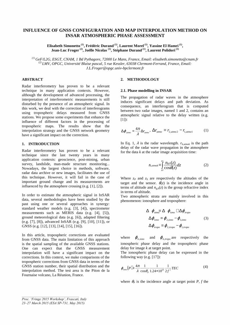
We use two COSMO-SkyMed HImage data acquired in ascending pass with VV polarization mode, an incidence angle of 40° and swath 15 (Tab. 1). Their acquisition dates frame the eruption that occurred June, 21 2014. The first image was acquired the 28th April 2014 during the warm and wet season. The second image was acquired on 9th July 2014 during the cold and dry season. The radar wavelength is equal to 3.12 cm (X-Band). The perpendicular baseline is around 27 m resulting in a height ambiguity of 396 m. Standard InSAR processing is performed using the DORIS software [22] and SNAPHU [23] for the phase unwrapping. A 4x4 multilook leads to a ground pixel size of around 8 m (Fig. 2). Topography is compensated using a LIDAR DEM with a grid mesh size of 7.5 m.

1 https://wwwobs.univ-bpclermont.fr/casoar/casoar_info.php, accessed in March 2015 2 http://wwwobs.univ-bpclermont.fr/SO/televolc/volinsar/index.php, accessed in March 2015 3 http://www.ipgp.fr/fr/ovpf/observatoire-volcanologique-piton-de-fournaise, accessed in March 2015 4 http://volobsis.ipgp.fr/index.php?page=home, accessed in March 2015

Date Satellite Orbit 04/28/2104 S1 37268 07/09/2014 S2 35609

Table 1. Data characteristics

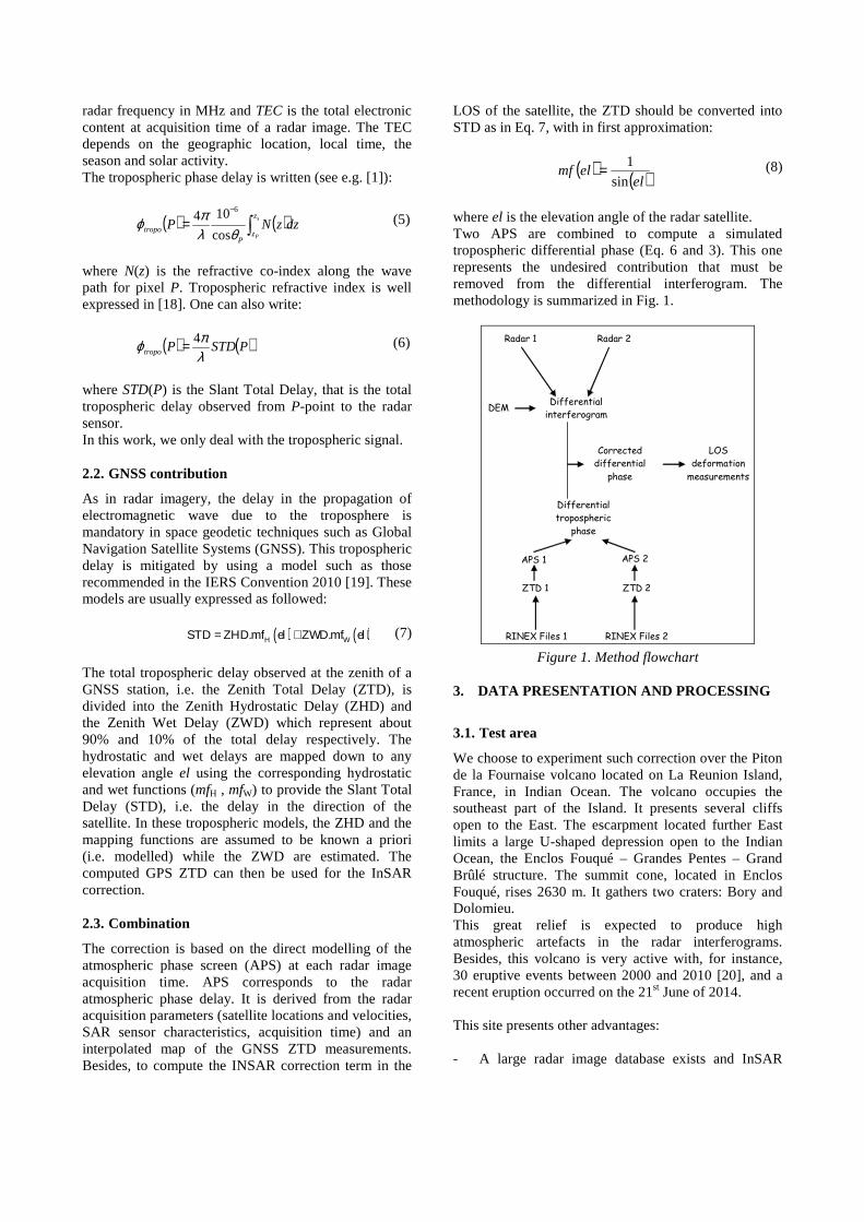
The coherence image shows a good level around the summit but is more irregular in the area named Grandes Pentes (eastern flank, Fig. 3). The differential phase in Fig. 4 reveals two superimposed patterns of fringes : 1) a short-wavelength bilobate pattern centered on the summit cone corresponds to the displacement induced by the June 2014 eruption and 2) a larger pattern of 7 – 8 fringes on the eastern flank of the volcano (Grandes Pentes – Grand Brûlé area) with a decreasing phase from the eastern base of the summit cone to the sea which corresponds to around 12 cm of LOS displacement away from the satellite. This pattern seems correlated with the terrain.

Figure 2. Amplitude image

Figure 3. Coherence image

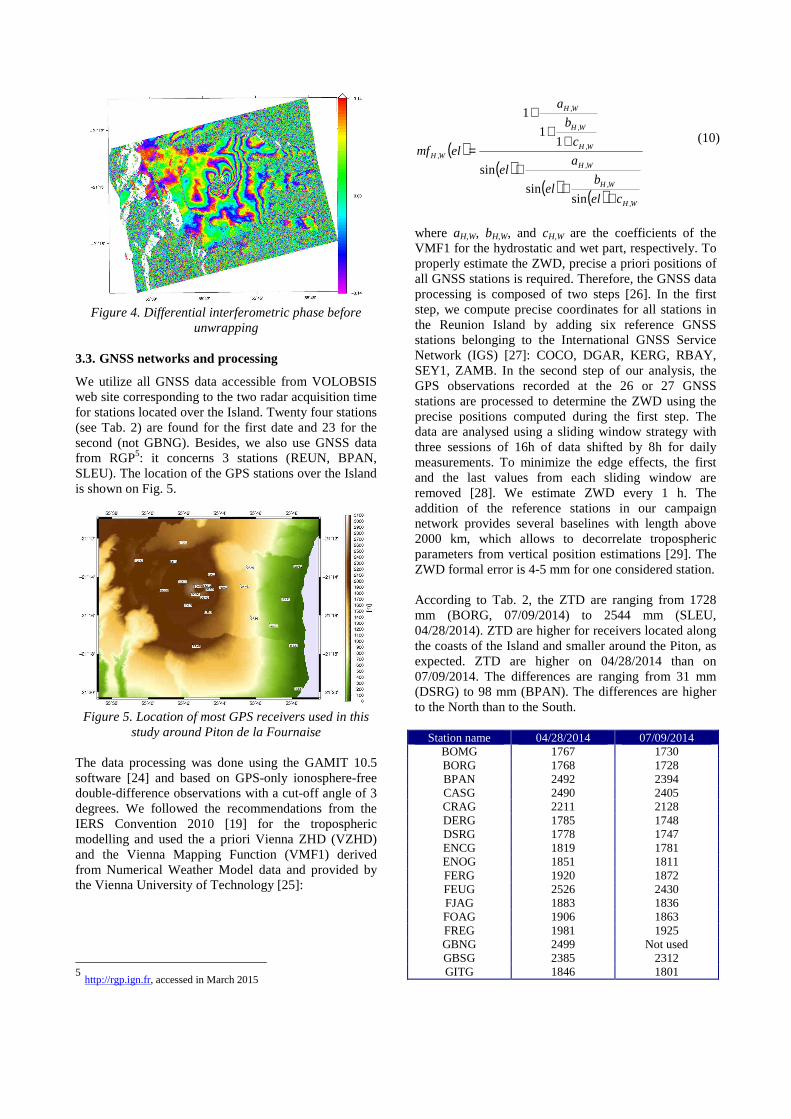
Figure 4. Differential interferometric phase before

unwrapping 3.3. GNSS networks and processing

We utilize all GNSS data accessible from VOLOBSIS web site corresponding to the two radar acquisition time for stations located over the Island. Twenty four stations (see Tab. 2) are found for the first date and 23 for the second (not GBNG). Besides, we also use GNSS data from RGP5: it concerns 3 stations (REUN, BPAN, SLEU). The location of the GPS stations over the Island is shown on Fig. 5.

Figure 5. Location of most GPS receivers used in this

study around Piton de la Fournaise The data processing was done using the GAMIT 10.5 software [24] and based on GPS-only ionosphere-free double-difference observations with a cut-off angle of 3 degrees. We followed the recommendations from the IERS Convention 2010 [19] for the tropospheric modelling and used the a priori Vienna ZHD (VZHD) and the Vienna Mapping Function (VMF1) derived from Numerical Weather Model data and provided by the Vienna University of Technology [25]:

5 http://rgp.ign.fr, accessed in March 2015

( )( )

( ) ( ) WH

WH

WH

WH

WH

WH

WH

cel

bel

ael

c

b

a

elmf

,

,

,

,

,

,

,

sinsin

sin

11

1

++

+

++

+

= (10)

where aH,W, bH,W, and cH,W are the coefficients of the VMF1 for the hydrostatic and wet part, respectively. To properly estimate the ZWD, precise a priori positions of all GNSS stations is required. Therefore, the GNSS data processing is composed of two steps [26]. In the first step, we compute precise coordinates for all stations in the Reunion Island by adding six reference GNSS stations belonging to the International GNSS Service Network (IGS) [27]: COCO, DGAR, KERG, RBAY, SEY1, ZAMB. In the second step of our analysis, the GPS observations recorded at the 26 or 27 GNSS stations are processed to determine the ZWD using the precise positions computed during the first step. The data are analysed using a sliding window strategy with three sessions of 16h of data shifted by 8h for daily measurements. To minimize the edge effects, the first and the last values from each sliding window are removed [28]. We estimate ZWD every 1 h. The addition of the reference stations in our campaign network provides several baselines with length above 2000 km, which allows to decorrelate tropospheric parameters from vertical position estimations [29]. The ZWD formal error is 4-5 mm for one considered station. According to Tab. 2, the ZTD are ranging from 1728 mm (BORG, 07/09/2014) to 2544 mm (SLEU, 04/28/2014). ZTD are higher for receivers located along the coasts of the Island and smaller around the Piton, as expected. ZTD are higher on 04/28/2014 than on 07/09/2014. The differences are ranging from 31 mm (DSRG) to 98 mm (BPAN). The differences are higher to the North than to the South.

Station name 04/28/2014 07/09/2014 BOMG 1767 1730 BORG 1768 1728 BPAN 2492 2394 CASG 2490 2405 CRAG 2211 2128 DERG 1785 1748 DSRG 1778 1747 ENCG 1819 1781 ENOG 1851 1811 FERG 1920 1872 FEUG 2526 2430 FJAG 1883 1836 FOAG 1906 1863 FREG 1981 1925 GBNG 2499 Not used GBSG 2385 2312 GITG 1846 1801

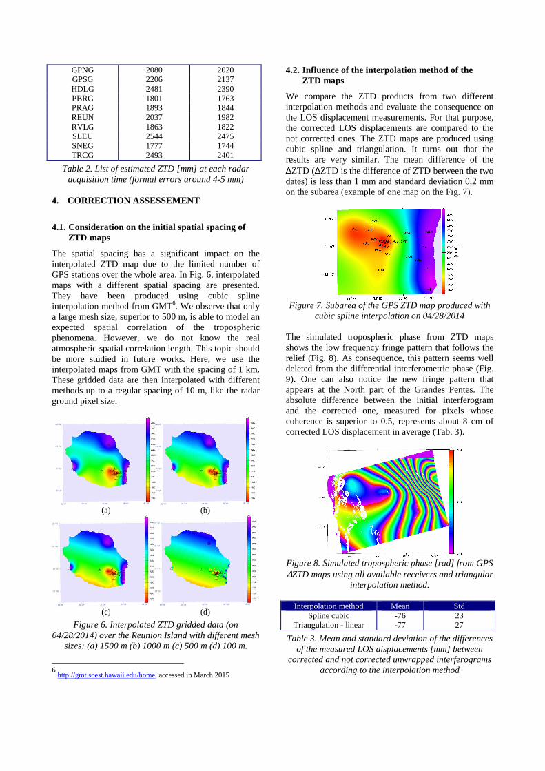
GPNG 2080 2020 GPSG 2206 2137 HDLG 2481 2390 PBRG 1801 1763 PRAG 1893 1844 REUN 2037 1982 RVLG 1863 1822 SLEU 2544 2475 SNEG 1777 1744 TRCG 2493 2401

Table 2. List of estimated ZTD [mm] at each radar acquisition time (formal errors around 4-5 mm)

4. CORRECTION ASSESSEMENT

4.1. Consideration on the initial spatial spacing of

ZTD maps

The spatial spacing has a significant impact on the interpolated ZTD map due to the limited number of GPS stations over the whole area. In Fig. 6, interpolated maps with a different spatial spacing are presented. They have been produced using cubic spline interpolation method from GMT6. We observe that only a large mesh size, superior to 500 m, is able to model an expected spatial correlation of the tropospheric phenomena. However, we do not know the real atmospheric spatial correlation length. This topic should be more studied in future works. Here, we use the interpolated maps from GMT with the spacing of 1 km. These gridded data are then interpolated with different methods up to a regular spacing of 10 m, like the radar ground pixel size.

(a) (b)

(c) (d)

Figure 6. Interpolated ZTD gridded data (on 04/28/2014) over the Reunion Island with different mesh

sizes: (a) 1500 m (b) 1000 m (c) 500 m (d) 100 m.

6 http://gmt.soest.hawaii.edu/home, accessed in March 2015

4.2. Influence of the interpolation method of the ZTD maps

We compare the ZTD products from two different interpolation methods and evaluate the consequence on the LOS displacement measurements. For that purpose, the corrected LOS displacements are compared to the not corrected ones. The ZTD maps are produced using cubic spline and triangulation. It turns out that the results are very similar. The mean difference of the ∆ZTD (∆ZTD is the difference of ZTD between the two dates) is less than 1 mm and standard deviation 0,2 mm on the subarea (example of one map on the Fig. 7).

Figure 7. Subarea of the GPS ZTD map produced with

cubic spline interpolation on 04/28/2014 The simulated tropospheric phase from ZTD maps shows the low frequency fringe pattern that follows the relief (Fig. 8). As consequence, this pattern seems well deleted from the differential interferometric phase (Fig. 9). One can also notice the new fringe pattern that appears at the North part of the Grandes Pentes. The absolute difference between the initial interferogram and the corrected one, measured for pixels whose coherence is superior to 0.5, represents about 8 cm of corrected LOS displacement in average (Tab. 3).

Figure 8. Simulated tropospheric phase [rad] from GPS ∆ZTD maps using all available receivers and triangular

interpolation method.

Interpolation method Mean Std Spline cubic -76 23

Triangulation - linear -77 27

Table 3. Mean and standard deviation of the differences of the measured LOS displacements [mm] between

corrected and not corrected unwrapped interferograms according to the interpolation method

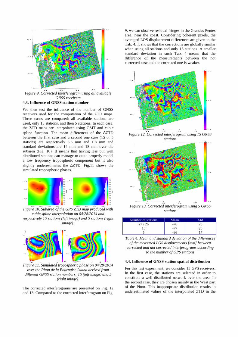
Figure 9. Corrected Interferogram using all available

GNSS receivers 4.3. Influence of GNSS station number

We then test the influence of the number of GNSS receivers used for the computation of the ZTD maps. Three cases are compared: all available stations are used, only 15 stations, and then 5 stations. In each case, the ZTD maps are interpolated using GMT and cubic spline function. The mean differences of the ∆ZTD between the first case and a second one case (15 or 5 stations) are respectively 3.5 mm and 1.8 mm and standard deviations are 14 mm and 18 mm over the subarea (Fig. 10). It means that having less but well distributed stations can manage to quite properly model a low frequency tropospheric component but it also slightly underestimates the ∆ZTD. Fig.11 shows the simulated tropospheric phases.

Figure 10. Subarea of the GPS ZTD map produced with

cubic spline interpolation on 04/28/2014 and respectively 15 stations (left image) and 5 stations (right

image).

Figure 11. Simulated tropospheric phase on 04/28/2014

over the Piton de la Fournaise Island derived from different GNSS station numbers: 15 (left image) and 5

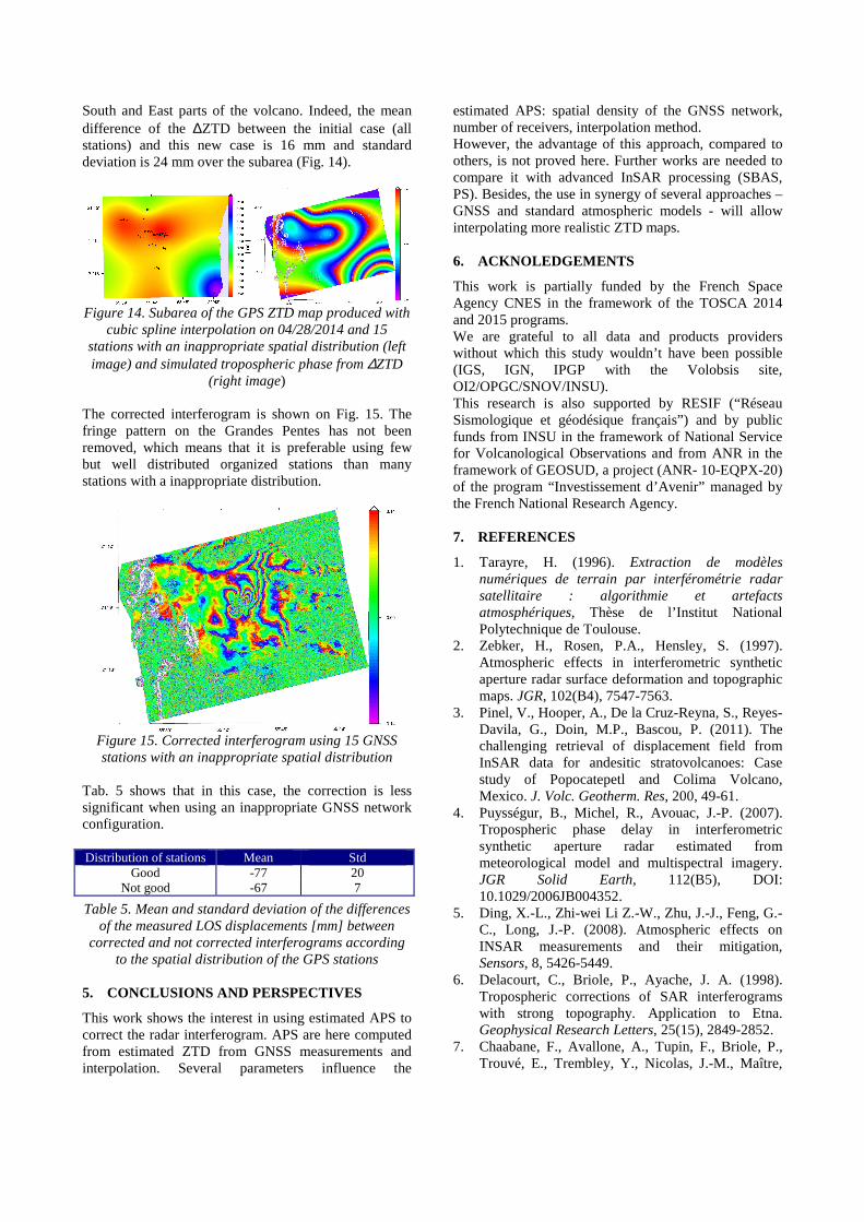
(right image). The corrected interferograms are presented on Fig. 12 and 13. Compared to the corrected interferogram on Fig.

9, we can observe residual fringes in the Grandes Pentes area, near the coast. Considering coherent pixels, the averaged LOS displacement differences are given in the Tab. 4. It shows that the corrections are globally similar when using all stations and only 15 stations. A smaller standard deviation in such Tab. 4 means that the difference of the measurements between the not corrected case and the corrected one is weaker.

Figure 12. Corrected interferogram using 15 GNSS

stations

Figure 13. Corrected interferogram using 5 GNSS

stations

Number of stations Mean Std 27 / 26 -76 23

15 -77 20 5 -86 17

Table 4. Mean and standard deviation of the differences of the measured LOS displacements [mm] between

corrected and not corrected interferograms according to the number of GPS stations

4.4. Influence of GNSS station spatial distribution

For this last experiment, we consider 15 GPS receivers. In the first case, the stations are selected in order to constitute a well distributed network over the area. In the second case, they are chosen mainly in the West part of the Piton. This inappropriate distribution results in underestimated values of the interpolated ZTD in the

South and East parts of the volcano. Indeed, the mean difference of the ∆ZTD between the initial case (all stations) and this new case is 16 mm and standard deviation is 24 mm over the subarea (Fig. 14).

Figure 14. Subarea of the GPS ZTD map produced with

cubic spline interpolation on 04/28/2014 and 15 stations with an inappropriate spatial distribution (left image) and simulated tropospheric phase from ∆ZTD

(right image) The corrected interferogram is shown on Fig. 15. The fringe pattern on the Grandes Pentes has not been removed, which means that it is preferable using few but well distributed organized stations than many stations with a inappropriate distribution.

Figure 15. Corrected interferogram using 15 GNSS stations with an inappropriate spatial distribution

Tab. 5 shows that in this case, the correction is less significant when using an inappropriate GNSS network configuration. Distribution of stations Mean Std

Good -77 20 Not good -67 7

Table 5. Mean and standard deviation of the differences of the measured LOS displacements [mm] between

corrected and not corrected interferograms according to the spatial distribution of the GPS stations

5. CONCLUSIONS AND PERSPECTIVES

This work shows the interest in using estimated APS to correct the radar interferogram. APS are here computed from estimated ZTD from GNSS measurements and interpolation. Several parameters influence the

estimated APS: spatial density of the GNSS network, number of receivers, interpolation method. However, the advantage of this approach, compared to others, is not proved here. Further works are needed to compare it with advanced InSAR processing (SBAS, PS). Besides, the use in synergy of several approaches – GNSS and standard atmospheric models - will allow interpolating more realistic ZTD maps. 6. ACKNOLEDGEMENTS

This work is partially funded by the French Space Agency CNES in the framework of the TOSCA 2014 and 2015 programs. We are grateful to all data and products providers without which this study wouldn’t have been possible (IGS, IGN, IPGP with the Volobsis site, OI2/OPGC/SNOV/INSU). This research is also supported by RESIF (“Réseau Sismologique et géodésique français”) and by public funds from INSU in the framework of National Service for Volcanological Observations and from ANR in the framework of GEOSUD, a project (ANR- 10-EQPX-20) of the program “Investissement d’Avenir” managed by the French National Research Agency. 7. REFERENCES

1. Tarayre, H. (1996). Extraction de modèles numériques de terrain par interférométrie radar satellitaire : algorithmie et artefacts atmosphériques, Thèse de l’Institut National Polytechnique de Toulouse.

2. Zebker, H., Rosen, P.A., Hensley, S. (1997). Atmospheric effects in interferometric synthetic aperture radar surface deformation and topographic maps. JGR, 102(B4), 7547-7563.

3. Pinel, V., Hooper, A., De la Cruz-Reyna, S., Reyes-Davila, G., Doin, M.P., Bascou, P. (2011). The challenging retrieval of displacement field from InSAR data for andesitic stratovolcanoes: Case study of Popocatepetl and Colima Volcano, Mexico. J. Volc. Geotherm. Res, 200, 49-61.

4. Puysségur, B., Michel, R., Avouac, J.-P. (2007). Tropospheric phase delay in interferometric synthetic aperture radar estimated from meteorological model and multispectral imagery. JGR Solid Earth, 112(B5), DOI: 10.1029/2006JB004352.

5. Ding, X.-L., Zhi-wei Li Z.-W., Zhu, J.-J., Feng, G.-C., Long, J.-P. (2008). Atmospheric effects on INSAR measurements and their mitigation, Sensors, 8, 5426-5449.

6. Delacourt, C., Briole, P., Ayache, J. A. (1998). Tropospheric corrections of SAR interferograms with strong topography. Application to Etna. Geophysical Research Letters, 25(15), 2849-2852.

7. Chaabane, F., Avallone, A., Tupin, F., Briole, P., Trouvé, E., Trembley, Y., Nicolas, J.-M., Maître,

H. (2002). Improvement of the tropospheric correction by adapted phase filtering. EUSAR, Cologne.

8. Bekeart, D.P.S., Hooper, A., Wright, T.J. (2015). A spatially variable power law tropospheric correction technique for InSAR data. JGR Solid Earth, 120, doi:10.1002/2014JB011558.

9. Ferretti, A., Prati, C., Rocca, F. (2001). Permanent scatterers in SAR Interferometry, IEEE TGRS, 39(1), 8 –20.

10. Hooper, A., Segall, P., Zebker, H. (2007). Persistent Scatterer InSAR for Crustal Deformation Analysis, With Application to Volcán Alcedo. JGR, 112(B07407), doi:10.1029/2006JB004763.

11. Berardino, P., Fornaro, G., Lanari, R., Sansosti, E. (2002). A new Algorithm for Surface Deformation Monitoring based on Small Baseline Differential SAR Interferograms. IEEE TGRS, 40(11), 2375-2383.

12. Williams, S., Bock, Y., Fang P. (1998). Integrated satellite interferometry: Tropospheric noise, GPS estimates and implications for interferometric synthetic aperture radar products, JGR, 103(27), doi:10.1029/98JB02794.

13. Onn, F., Zebker, H. (2006). Correction for interferometric synthetic aperture radar atmospheric phase artifacts using time series of zenith wet delay observations from a GPS network. JGR, 111(B09102), doi:10.1029/2005JB004012.

14. Ge, L., Han, S., Rizos, C. (2000). The double interpolation and double prediction (DIDP) approach for INSAR and GPS integration. IAPRS, vol.XXXIII, Amsterdam.

15. Janssen, V., Ge, L., Rizos, C. (2004). Tropospheric correction to SAR interferometry from GPS observations, GPS Solutions, 8, 140-151.

16. Xu, C. et al. (2006). InSAR tropospheric delay mitigation by GPS observations: A case study in Tokyo area. J. of Atmospheric and Solar-Terrestrial Physics, 68, 629-638.

17. Ducic, V. (2004). Tomographie de l’ionosphère et de la troposphère à partir de données GPS denses. Applications aux risques naturels et amélioration de l’interférométrie SAR. Thèse de l’Université de Paris 7.

18. Smith, E. K., Weintraub, S. (1953). The constants in the equation for atmospheric refractive index at radio frequencies, J. Res. Natl. Bur. Stand., 50, 39-41.

19. Petit, G., et al. (2010). IERS Conventions (IERS Technical Note ; 36) Frankfurt am Main: Verlag des Bundesamts für Kartographie und Geodäsie, ISBN 3-89888-989-6.

20. Brenguier, F., et al. (2012). First Results from the UnderVolc High Resolution Seismic and GPS Network Deployed on Piton de la Fournaise Volcano. Seismological Research Letters, 83(1), 97-102.

21. Froger, J.-L., Souriot, T., Villeneuve, N., Rabaute, T., Durand, P., Cayol, V., Di Muro, A., Staudacher, T., Fruneau, B. (2012). Apport des données Terrasar-X pour le suivi de l’activité du Piton de la Fournaise. Revue Française de Photogrammétrie et Télédétection, 197, 86-101.

22. Kampes, B.M., et al. (2003). Radar interferometry with public domain tools. Third International Workshop FRINGE03, Frascati, Italy.

23. Chen, C.W., Zebker, H.A. (2002). Phase unwrapping for large SAR interferograms: Statistical segmentation and generalized network models. IEEE TGRS, 40, 1709-1719.

24. Herring, T.A., King, R.W., McKlusky, S.C. (2010). Reference manual for the GAMIT GPS software, release, 10.3. Department of Earth, Atmospheric, and Planetary Sciences, Massachusetts Institute of Technology, Boston, USA.

25. Boehm, J., Werl, B., Schuh, H. (2006). Troposphere mapping functions for GPS and very long baseline interferometry from European Centre for Medium-Range Weather Forecasts operational analysis data. JGR Solid Earth, 111(B02406).

26. Morel, L., Pottiaux, E., Durand, F., Fund, F., Boniface, K., de Oliveira, P.-S., Van Baelen, J. (2015). Validity and behaviour of tropospheric gradients estimated by GPS in Corsica. Adv. Space Res., 135(1), 135-149.

27. Dow, J., Neilan, E., Rizos, C. (2009). The International GNSS Service in a changing landscape of Global Navigation Satellite Systems. J. Geod., 83(3), 191-198.

28. Jin, S., Park, J.U., Cho, J.H., Park, P.H. (2007). Seasonal variability of GPS derived zenith tropospheric delay (1994 – 2006) and climate implications. JGR Atmospheres. 112(D9).

29. Tregoning, P., Boers, R., O’Brien, D., Hendy, M. (1998). Accuracy of Absolute Precipitable Water Vapor Estimates from GPS Observations. JGR; 103, 28701–28710, doi:10.1029/98JD02516.