Influence of environmental variables on stream fish fauna

Neotropical Ichthyology, 14(3): e150116, 2016 DOI: 10.1590/1982-0224-20150116

Journal homepage: www.scielo.br/niPublished online: 15 September 2016 (ISSN 1982-0224)

1

Influence of environmental variables on stream fish fauna at multiple spatial scales

Nara Tadini Junqueira1, Diego Rodrigues Macedo2,3, Rafael Couto Rosa de Souza1, Robert Mason Hughes1,4, Marcos Callisto2 and Paulo Santos Pompeu1

Effects of environmental variables at different spatial scales on freshwater fish assemblages are relatively unexplored in Neotropical ecosystems. However, those influences are important for developing management strategies to conserve fish diversity and water resources. We evaluated the influences of site- (in-stream) and catchment-scale (land use and cover) environmental variables on the abundance and occurrence of fish species in streams of the Upper Araguari River basin through use of variance partitioning with partial CCA. We sampled 38 1st to 3rd order stream sites in September 2009. We quantified site variables to calculate 11 physical habitat metrics and mapped catchment land use/cover. Site and catchment variables explained > 50% of the total variation in fish species. Site variables (fish abundance: 25.31%; occurrence: 24.51%) explained slightly more variation in fish species than catchment land use/cover (abundance: 22.69%; occurrence: 18.90%), indicating that factors at both scales are important. Because anthropogenic pressures at site and catchment scales both affect stream fish in the Upper Araguari River basin, both must be considered jointly to apply conservation strategies in an efficient manner.

Os efeitos das variáveis ambientais em diferentes escalas espaciais sobre as assembleias de peixes de água doce ainda é um tema pouco explorado na região Neotropical. Entretanto é um assunto de extrema relevância, pois gera subsídios para definições de estratégias de manejo e conservação de ictiofauna e dos recursos hídricos. Nós avaliamos a influência de variáveis ambientais em escalas local (dentro do rio) e da paisagem (uso e cobertura do solo) na abundância e ocorrência das espécies de peixes de riachos da bacia do alto rio Araguari através da partição da variância usando CCA parcial. Um total de 38 riachos de até 3ª ordem foi amostrado em setembro de 2009. Nós quantificamos variáveis locais para calcular 11 métricas de hábitats físicos e mapeamos o uso e cobertura do solo. O conjunto de dados (variáveis locais e da paisagem) explicou mais de 50% da variação total nas espécies de peixes. Variáveis em escala local (abundância: 25,31%; ocorrência: 24,51%) explicaram levemente uma maior variação nas assembleias de peixes do que o uso e cobertura do solo (abundância: 22,69%; ocorrência: 18,90%), indicando que os fatores em ambas as escalas de estudo são importantes. Uma vez que a influência antrópica em diferentes escalas afeta as espécies de peixes em riachos da bacia do alto rio Araguari, ambas devem ser consideradas juntamente para a adoção de estratégias de conservação de uma forma racional.

Keywords: Disturbed sites, Fish assemblages, Land use, Partial CCA, Physical habitat.

1Departamento de Biologia, Universidade Federal de Lavras (UFLA), 37200-000 Lavras, MG, Brazil. (NTJ) [email protected] (corresponding author), (RCRS) [email protected], (PSP) [email protected]ório de Ecologia de Bentos, Departamento de Biologia Geral, Universidade Federal de Minas Gerais (UFMG), Av. Antônio Carlos, 6627, 31270-901 Belo Horizonte, MG, Brazil. (MC) [email protected] 3Departamento de Geografia, Instituto de Geociências, Universidade Federal de Minas Gerais (UFMG), Av. Antônio Carlos, 6627, 31270-901 Belo Horizonte, MG, Brazil. (DRM) [email protected] 4Amnis Opes Institute and Department of Fisheries and Wildlife, Oregon State University (OSU), 2895 SE Glenn, Corvallis, OR, 97333, USA. [email protected]

Introduction

Streams are hierarchically organized and spatially nested systems (Frissell et al., 1986 in which conditions at smaller spatial scales are constrained by processes at larger spatial scales (O’Neill et al., 1989). In other words, site conditions are influenced by regional conditions

(Hildrew & Giller, 1994), and different variables may act at different scales (Willis & Whittaker, 2002). Some stream processes operate primarily at regional scales, such as channel form and hydrology (Poff & Allan, 1995), but other stream conditions operate primarily at the site scale, such as habitat complexity and shade (Allan et al., 1997).

Variables at multiple scales and ichthyofauna of streamsNeotropical Ichthyology, 14(3): e150116, 20162

The importance of the landscape to streams is associated with allochthonous and autochthonous resources and the surrounding terrestrial environment is the primary source of organic matter for many small, forested, temperate streams (Vannote et al., 1980; Wallace et al., 1997). Land use, such as urbanization and agriculture, strongly influences this linkage and changes flow regimes, temperature, water chemistry, and substrate characteristics (Schlosser & Karr, 1981; Peterjohn & Correll, 1984; Hughes et al., 2014). Consequently, they cause many environmental changes such as physical habitat loss, sedimentation, bank erosion and bed destabilization, contaminant loadings, canopy opening, and nutrient enrichment (Allan, 2004). Moreover, local habitat conditions are directly or indirectly affected by catchment conditions, including land use changes (e.g., Sály et al., 2011; Marzin et al., 2012; Macedo et al., 2014). Local habitat conditions are a fundamental factor for determining the structure and composition of stream biota (Schlosser, 1982; Rosenzweig, 1995; Harding et al., 1998; Brown et al., 2009). For example, fish assemblages are strongly influenced by site channel structure and hydraulic conditions, such as substrate, canopy shading, fish cover, wetted width, depth variation, and slope (Gorman & Karr, 1978; Wang et al., 1998; Kaufmann & Hughes, 2006). Land use changes, such as agriculture, remove riparian vegetation and decreases bank stabilization thereby increasing sedimentation. Sedimentation reduces stream depth heterogeneity, leading to decreased species diversity (Wood & Armitage, 1997; Sutherland et al., 2002). Therefore, those patterns and processes operating at local and regional scales play an important role in determining stream fish assemblage structure and complexity (Matthews, 1998), and both are affected by human activities.

The relative importance of catchment and site conditions to the structure of fish assemblages and the degree of anthropogenic pressure is, however, controversial. Some studies have suggested that in highly disturbed temperate catchments that are heavily dominated by anthropogenic land use/cover, the relative importance of site conditions for stream fish decline and catchment conditions prevail (Allan et al., 1997; Wang et al., 2006a), because anthropogenic pressures modify the processes that operated at different spatial scales (Moerke & Lamberti, 2006). On the other hand, in minimally disturbed temperate catchments, site conditions have greater importance (Kaufmann & Hughes, 2006; Wang et al., 2006b). However, contradictory results have been reported (e.g. Bouchard & Boisclair, 2007), including papers describing both catchment- and site-scale conditions with similar importance (e.g. Hughes et al., 2015). In addition, studies regarding the influence of environmental factors at different spatial scales on Neotropical stream biota are still scant. Understanding these relationships is an important step for taking appropriate stream conservation and management actions (Wang et al., 2006b). By doing so, the main drivers of impacts can be identified and rehabilitation efforts can be

focused on the scales where management actions are most cost-effective.

We evaluated the association between environmental variables and the composition of fish assemblages in 38 wadeable streams in the Upper Araguari River Basin at two spatial scales: site and catchment. We addressed the question: How much variability in the composition of fish assemblages is explained by environmental variables at the site (physical habitat) and catchment (land use and cover) scales? Because our study area has relatively high levels of human land use (Ligeiro et al., 2013), it is an exploratory attempt to understand how Neotropical stream fishes respond to land use/cover and to site habitat conditions.

Material and Methods

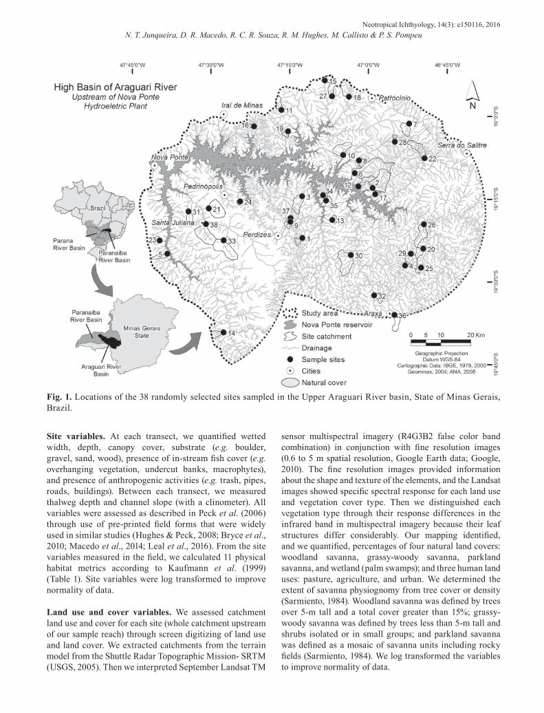
Study area and design. We conducted our study in wadeable first to third order streams in the Upper Araguari River basin, at the end of the dry season, September 2009 (Fig. 1). The Araguari River rises in the Serra da Canastra National Park, Minas Gerais, southeastern Brazil. The river is 475 km long and a major left tributary of the Paranaíba River (Baccarro et al., 2004), which forms the Upper Paraná River after its confluence with the Grande River. The study area was located upstream from Nova Ponte Dam (the streams flow into Nova Ponte Reservoir). The Nova Ponte hydropower plant is located in the Municipality of Nova Ponte, State of Minas Gerais (216790 S/ 7881847 E, Zone 23K) and it began operation in 1994. The total maximum volume of the reservoir is 12,792 hm³ and the flooded area is 449.24 km² (Cachapuz, 2006). The Upper Araguari River has well-defined seasons: a dry season from May to September and a rainy season from October to April (Rosa, 2004). The region produces considerable amounts of soy, coffee, corn, and sugar cane and has a well-developed irrigated agriculture system. Most people live in small towns with up to 20,000 inhabitants (Ligeiro et al., 2013).

We randomly selected 38 sampling sites (one site per stream). Site selection followed the generalized random tessellation stratified (GRTS) sampling design according to Stevens & Olsen (2004) and Olsen & Peck (2008). This is a probability-based design in which a master sample frame is established by using a digitized drainage system map, and then the sample sites are selected via hierarchical, spatially weighted criteria. We excluded all tributaries greater than Strahler order 3 on a digital 1:100,000 scale map because our targets were wadeable perennial streams. All stream channels located > 35 km from the shore of the Nova Ponte Reservoir were excluded to reduce travel distances and limit the effect of different fish species dispersal capacities (Hitt & Angermeier, 2008). The length of each sample site was 40 times its mean wetted width, with a minimum length of 150 m (Kaufmann et al., 1999). Each site was subdivided into 11 equally spaced transects.

N. T. Junqueira, D. R. Macedo, R. C. R. Souza, R. M. Hughes, M. Callisto & P. S. PompeuNeotropical Ichthyology, 14(3): e150116, 2016

3

Site variables. At each transect, we quantified wetted width, depth, canopy cover, substrate (e.g. boulder, gravel, sand, wood), presence of in-stream fish cover (e.g. overhanging vegetation, undercut banks, macrophytes), and presence of anthropogenic activities (e.g. trash, pipes, roads, buildings). Between each transect, we measured thalweg depth and channel slope (with a clinometer). All variables were assessed as described in Peck et al. (2006) through use of pre-printed field forms that were widely used in similar studies (Hughes & Peck, 2008; Bryce et al., 2010; Macedo et al., 2014; Leal et al., 2016). From the site variables measured in the field, we calculated 11 physical habitat metrics according to Kaufmann et al. (1999) (Table 1). Site variables were log transformed to improve normality of data.

Land use and cover variables. We assessed catchment land use and cover for each site (whole catchment upstream of our sample reach) through screen digitizing of land use and land cover. We extracted catchments from the terrain model from the Shuttle Radar Topographic Mission- SRTM (USGS, 2005). Then we interpreted September Landsat TM

sensor multispectral imagery (R4G3B2 false color band combination) in conjunction with fine resolution images (0.6 to 5 m spatial resolution, Google Earth data; Google, 2010). The fine resolution images provided information about the shape and texture of the elements, and the Landsat images showed specific spectral response for each land use and vegetation cover type. Then we distinguished each vegetation type through their response differences in the infrared band in multispectral imagery because their leaf structures differ considerably. Our mapping identified, and we quantified, percentages of four natural land covers: woodland savanna, grassy-woody savanna, parkland savanna, and wetland (palm swamps); and three human land uses: pasture, agriculture, and urban. We determined the extent of savanna physiognomy from tree cover or density (Sarmiento, 1984). Woodland savanna was defined by trees over 5-m tall and a total cover greater than 15%; grassy-woody savanna was defined by trees less than 5-m tall and shrubs isolated or in small groups; and parkland savanna was defined as a mosaic of savanna units including rocky fields (Sarmiento, 1984). We log transformed the variables to improve normality of data.

Fig. 1. Locations of the 38 randomly selected sites sampled in the Upper Araguari River basin, State of Minas Gerais, Brazil.


Table 1. Descriptions of 11 site attributes represented for acronyms according to Kaufmann et al. (1999).

Reach variables Description

Xwxd mean wetted width multiplied by depth (m²)Sddepth standard deviation of thalweg depth (cm)

Xcdenmid

average values of riparian canopy cover measured with a canopy densitometer from each transect and then convert to a percentage by dividing by 17 (the densiometer maximum amount of vegetation cover) and multiplying the result by 100

PCT_FN percentage of fine substrate (<0.06 mm, i.e., silt, clay and muck)

Lsub_dmm log10 [estimated geometric mean substrate diameter (mm)]

PCT_sfgf percentage of fine gravel and smaller (<16 mm) substrate

xfc_lwd sum of large wood debris areal coverxfc_brs sum of brush and small wood debris areal cover

xfc_natnatural fish cover. Sum of cover from large wood, brush, overhanging vegetation, boulders, and undercut banks

w1_hall

percentage of observations (11 transects x two banks = 22 observations in total) for each type of direct human disturbance (wall/dike, buildings, pavement, pipes, trash, mining activity, logging operations, pasture, row crops). Different weights were assigned for each spatial class: 1.5 to impact inside the channel or on the banks, 1.0 to impact within 10 meters from the banks, and 0.667 for impacts >10 meters from the banks. The sum of the results of all of the types of human impacts assessed at the site scale provided an estimate of local anthropogenic disturbance at the site

Xslope water surface gradient over reach (%)

Pure spatial variables. To take into account spatial autocorrelation of the data we included pure spatial variables in our analysis. We determined the geographical coordinates (latitude and longitude) of each site in the field using a GPS. In the laboratory, the geographical coordinates (latitude and longitude) of the sites were centered on their means to reduce collinearity among terms when fitting the regression (Legendre & Legendre, 2012). Next, we calculated a matrix of spatial data, with x = longitude (centered) and y = latitude (centered), by including all terms of a cubic trend surface regression. The terms included were: x, y, x², xy, y², x³, x²y, xy² and y³ (Legendre, 1990; Borcard et al., 1992). The spatial variables were log transformed.

Fish sampling. We sampled fish assemblages in an upstream direction with two hand nets made with plastic mosquito screen (1 mm mesh) attached to an 80 cm diameter hemispherical steel frame. Each site was sampled approximately for two hours (12 min in each transect), thoroughly lifting substrates and netting between each transect. The capture efficiency of this method was tested through various estimators, with efficiencies of 78-85% for both benthic and water column species (Leal et al., 2014). Fish were kept separately by sample site, anesthetized in

a solution of clove oil, and then fixed in 10% formalin. In the laboratory, all fish were washed in tap water, preserved in 70% alcohol, and identified to the species level, according to Graça & Pavanelli (2007). Voucher specimens are deposited in the ichthyological collection of the Universidade Federal de Lavras (CI-UFLA) and in the Museu de Zoologia da Universidade de São Paulo (MZUSP). We used Hellinger-transformed fish data.

Data analysis. We used the multivariate approach “partial constrained ordination” to estimate the variation in fish species occurrence and abundance explained by environmental conditions. We used a two-step approach for variance partitioning. First, we ran a detrended correspondence analysis (DCA) to test the gradient length of species composition and then to determine the appropriate constrained ordination technique (canonical correspondence analysis, CCA, or redundancy analysis, RDA). According to Braak (1995), data with < 2 standard deviations (SD) of turnover along the first DCA axis are likely to respond linearly to environmental gradients, and RDA should be used; data with > 2 SD of turnover are likely to respond unimodally, and CCA should be used. Our two fish datasets (abundance and occurrence) responded unimodally to environmental gradients (SD > 2), so we used CCA.

We then used variance partitioning with partial CCA to partition total variation in each fish dataset (abundance and occurrence) into components explained by land use/cover (land use), site (site), and pure spatial (spatial) predictors (Anderson & Gribble, 1998; Hughes et al., 2015). For this, we ran twelve CCAs for each fish dataset (Table 2) to partition total variation in eight components: i) pure land use, ii) pure spatial, iii) pure site, iv) shared land use and spatial variation, v) shared land use and site variation, vi) shared spatial and site variation, vii) variation between all three components, and viii) unexplained variation. Fractions iv, v and vi were obtained by subtraction and they are not fitted variance components. The percentage of total variation explained by each constrained (Table 2, CCAs 1 to 3) or partial ordination (Table 2, CCAs 4 to 12) was obtained by the sum of canonical eigenvalues of each run divided by the sum of all eigenvalues obtained by an unconstrained correspondence analysis (CA, species data), and multiplied by 100 (Borcard et al., 1992). The percentage of variation in the fish data sets explained by individual variables of partial CCAs (Table 2, CCAs 6, 9 and 12) was calculated from the ratio of Lambda A (extra fit) to the sum of all eigenvalues (total inertia), multiplied by 100. These CCAs represent the percentage of total variation explained exclusively by land use dataset (CCA 6), site dataset (CCA 9) and spatial dataset (CCA 12). All analyses were run in Canoco v. 4.0 for Windows (Braak & Smilauer, 1998), down weighting rare species, with automatic forward selection of environmental variables, and 1,000 permutations using partial Monte Carlo randomization tests.


5

Table 2. Step descriptions of the 12 CCAs run over fish abundance and incidence datasets.

Step descriptions

(1) CCA of fish matrix,constrained by the land use matrix

(2) CCA of fish matrix, constrained by the site matrix

(3) CCA of fish matrix, constrained by the pure spatial matrix

(4) CCA of fish matrix, constrained by the land use matrix, with site variables treated as covariables

(5) CCA of fish matrix, constrained by the land use matrix, with the pure spatial variables treated as covariables

(6) CCA of fish matrix, constrained by the land use matrix, with the site and pure spatial variables treated as covariables

(7) CCA of fish matrix, constrained by the site matrix, with the land use variables treated as covariables

(8) CCA of fish matrix, constrained by the site matrix, with the pure spatial variables treated as covariables

(9) CCA of fish matrix, constrained by the site matrix, with the land use and pure spatial variables treated as covariables

(10) CCA of fish matrix, constrained by the pure spatial matrix, with the land use variables treated as covariables

(11) CCA of fish matrix, constrained by the pure spatial matrix, with the site variables treated as covariables

(12) CCA of fish matrix, constrained by the pure spatial matrix, with the land use and site variables treated as covariables

Results

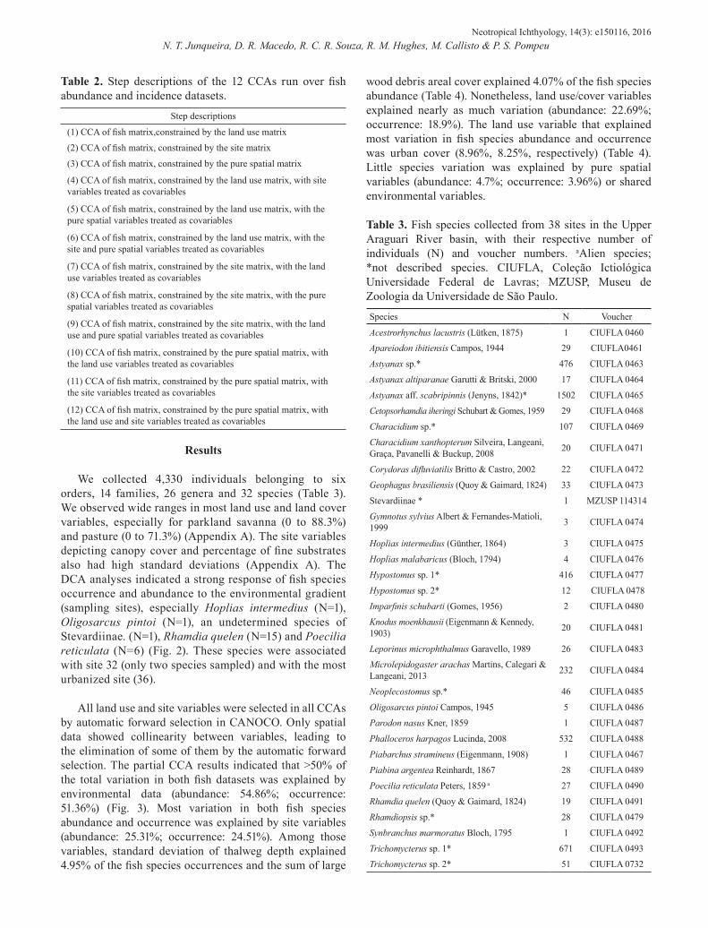
We collected 4,330 individuals belonging to six orders, 14 families, 26 genera and 32 species (Table 3). We observed wide ranges in most land use and land cover variables, especially for parkland savanna (0 to 88.3%) and pasture (0 to 71.3%) (Appendix A). The site variables depicting canopy cover and percentage of fine substrates also had high standard deviations (Appendix A). The DCA analyses indicated a strong response of fish species occurrence and abundance to the environmental gradient (sampling sites), especially Hoplias intermedius (N=1), Oligosarcus pintoi (N=1), an undetermined species of Stevardiinae. (N=1), Rhamdia quelen (N=15) and Poecilia reticulata (N=6) (Fig. 2). These species were associated with site 32 (only two species sampled) and with the most urbanized site (36).

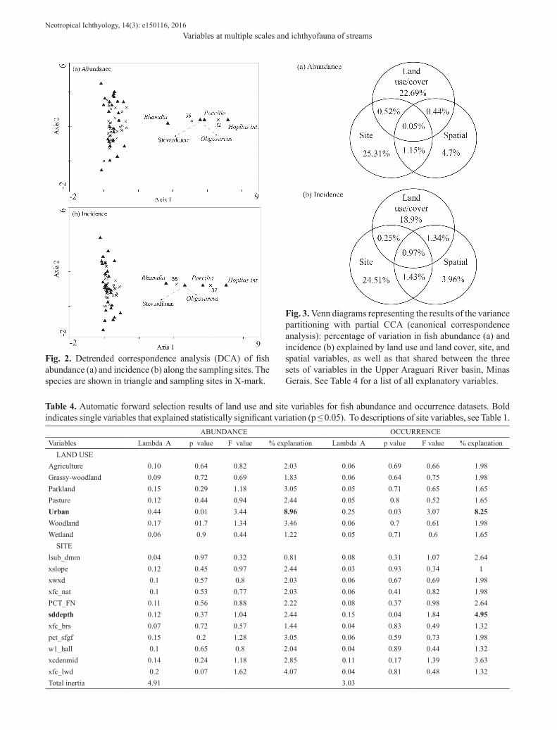
All land use and site variables were selected in all CCAs by automatic forward selection in CANOCO. Only spatial data showed collinearity between variables, leading to the elimination of some of them by the automatic forward selection. The partial CCA results indicated that >50% of the total variation in both fish datasets was explained by environmental data (abundance: 54.86%; occurrence: 51.36%) (Fig. 3). Most variation in both fish species abundance and occurrence was explained by site variables (abundance: 25.31%; occurrence: 24.51%). Among those variables, standard deviation of thalweg depth explained 4.95% of the fish species occurrences and the sum of large

wood debris areal cover explained 4.07% of the fish species abundance (Table 4). Nonetheless, land use/cover variables explained nearly as much variation (abundance: 22.69%; occurrence: 18.9%). The land use variable that explained most variation in fish species abundance and occurrence was urban cover (8.96%, 8.25%, respectively) (Table 4). Little species variation was explained by pure spatial variables (abundance: 4.7%; occurrence: 3.96%) or shared environmental variables.

Table 3. Fish species collected from 38 sites in the Upper Araguari River basin, with their respective number of individuals (N) and voucher numbers. aAlien species; *not described species. CIUFLA, Coleção Ictiológica Universidade Federal de Lavras; MZUSP, Museu de Zoologia da Universidade de São Paulo.

Species N Voucher

Acestrorhynchus lacustris (Lütken, 1875) 1 CIUFLA 0460Apareiodon ibitiensis Campos, 1944 29 CIUFLA0461

Astyanax sp.* 476 CIUFLA 0463

Astyanax altiparanae Garutti & Britski, 2000 17 CIUFLA 0464

Astyanax aff. scabripinnis (Jenyns, 1842)* 1502 CIUFLA 0465

Cetopsorhamdia iheringi Schubart & Gomes, 1959 29 CIUFLA 0468

Characidium sp.* 107 CIUFLA 0469Characidium xanthopterum Silveira, Langeani, Graça, Pavanelli & Buckup, 2008 20 CIUFLA 0471

Corydoras difluviatilis Britto & Castro, 2002 22 CIUFLA 0472

Geophagus brasiliensis (Quoy & Gaimard, 1824) 33 CIUFLA 0473

Stevardiinae * 1 MZUSP 114314Gymnotus sylvius Albert & Fernandes-Matioli, 1999 3 CIUFLA 0474

Hoplias intermedius (Günther, 1864) 3 CIUFLA 0475

Hoplias malabaricus (Bloch, 1794) 4 CIUFLA 0476

Hypostomus sp. 1* 416 CIUFLA 0477

Hypostomus sp. 2* 12 CIUFLA 0478

Imparfinis schubarti (Gomes, 1956) 2 CIUFLA 0480Knodus moenkhausii (Eigenmann & Kennedy, 1903) 20 CIUFLA 0481

Leporinus microphthalmus Garavello, 1989 26 CIUFLA 0483Microlepidogaster arachas Martins, Calegari & Langeani, 2013 232 CIUFLA 0484

Neoplecostomus sp.* 46 CIUFLA 0485

Oligosarcus pintoi Campos, 1945 5 CIUFLA 0486

Parodon nasus Kner, 1859 1 CIUFLA 0487

Phalloceros harpagos Lucinda, 2008 532 CIUFLA 0488

Piabarchus stramineus (Eigenmann, 1908) 1 CIUFLA 0467

Piabina argentea Reinhardt, 1867 28 CIUFLA 0489

Poecilia reticulata Peters, 1859 a 27 CIUFLA 0490

Rhamdia quelen (Quoy & Gaimard, 1824) 19 CIUFLA 0491

Rhamdiopsis sp.* 28 CIUFLA 0479

Synbranchus marmoratus Bloch, 1795 1 CIUFLA 0492

Trichomycterus sp. 1* 671 CIUFLA 0493Trichomycterus sp. 2* 51 CIUFLA 0732


Fig. 2. Detrended correspondence analysis (DCA) of fish abundance (a) and incidence (b) along the sampling sites. The species are shown in triangle and sampling sites in X-mark.

Table 4. Automatic forward selection results of land use and site variables for fish abundance and occurrence datasets. Bold indicates single variables that explained statistically significant variation (p ≤ 0.05). To descriptions of site variables, see Table 1. ABUNDANCE OCCURRENCEVariables Lambda A p value F value % explanation Lambda A p value F value % explanation

LAND USE Agriculture 0.10 0.64 0.82 2.03 0.06 0.69 0.66 1.98Grassy-woodland 0.09 0.72 0.69 1.83 0.06 0.64 0.75 1.98Parkland 0.15 0.29 1.18 3.05 0.05 0.71 0.65 1.65Pasture 0.12 0.44 0.94 2.44 0.05 0.8 0.52 1.65Urban 0.44 0.01 3.44 8.96 0.25 0.03 3.07 8.25Woodland 0.17 01.7 1.34 3.46 0.06 0.7 0.61 1.98Wetland 0.06 0.9 0.44 1.22 0.05 0.71 0.6 1.65

SITE lsub_dmm 0.04 0.97 0.32 0.81 0.08 0.31 1.07 2.64xslope 0.12 0.45 0.97 2.44 0.03 0.93 0.34 1xwxd 0.1 0.57 0.8 2.03 0.06 0.67 0.69 1.98xfc_nat 0.1 0.53 0.77 2.03 0.06 0.41 0.82 1.98PCT_FN 0.11 0.56 0.88 2.22 0.08 0.37 0.98 2.64sddepth 0.12 0.37 1.04 2.44 0.15 0.04 1.84 4.95xfc_brs 0.07 0.72 0.57 1.44 0.04 0.83 0.49 1.32pct_sfgf 0.15 0.2 1.28 3.05 0.06 0.59 0.73 1.98w1_hall 0.1 0.65 0.8 2.04 0.04 0.89 0.44 1.32xcdenmid 0.14 0.24 1.18 2.85 0.11 0.17 1.39 3.63xfc_lwd 0.2 0.07 1.62 4.07 0.04 0.81 0.48 1.32Total inertia 4.91 3.03

Fig. 3. Venn diagrams representing the results of the variance partitioning with partial CCA (canonical correspondence analysis): percentage of variation in fish abundance (a) and incidence (b) explained by land use and land cover, site, and spatial variables, as well as that shared between the three sets of variables in the Upper Araguari River basin, Minas Gerais. See Table 4 for a list of all explanatory variables.


7

Discussion

The set of site variables explained more variation in our fish dataset than catchment variables. Similar results have been reported from studies in temperate regions (Wang et al., 2003; Johnson et al., 2007; Bouchard & Boisclair, 2007). We believe that our study scale contributed to this result. The different scale of study designs coupled with differences in the scale of dependency of certain process (e.g. organic matter input and sediment delivery) influence the contrasting results in the literature (Allan & Johnson, 1997; Wang et al., 2006b). Generally, one has a greater ability to detect site conditions but less ability to detect regional effects when more sites are sampled per catchment versus sampling more catchments with fewer sites in each (Wang et al., 2006b). We studied only the Upper Araguari River basin, in the Cerrado Domain, and many sites were located close to each other. Therefore, our scale of measurement is likely more sensitive to effects of site variables on fish assemblages.

Influence of site factors such as habitat structure on fish assemblages has been investigated extensively (Schlosser, 1982; Harding et al., 1998; Kaufmann & Hughes, 2006; Brown et al., 2009). The structure of stream fish assemblages has been related to numerous site variables, such as bottom type and cover (Angermeier & Winston, 1998), and bottom, depth, and current (Gorman & Karr, 1978). In our study, standard deviation of thalweg depth individually was the most important site variable related to fish occurrence. The standard deviation of thalweg depth is a quantitative measure of relatively flow-independent channel morphology, and it is considered an index of bottom complexity (Kaufmann et al., 1999). Thus, higher values are related to increased bottom complexity, with heterogeneous substrate size and hydraulic regimes, providing living space and cover for fish species with different preferences, affecting fish occurrence. For example, when fine sediment is predominant, the occurrence of habitat specialists, like benthic Loricariidae, can be negatively affected (Waters, 1995), because such species inhabit runs and riffles and are specialist benthic feeders (Terra et al., 2015). Furthermore, field measurements of thalweg depth are recommended for monitoring programs (Kaufmann et al., 1999) because the variability of this attribute can be drastically reduced by sedimentation. For fish species abundance, the site variable “sum of large wood areal cover” explained most variation. Large wood is abundant in many undisturbed stream ecosystems and plays key functions: dissipation of flow energy, stabilization of channel banks, formation of pools (Booth et al., 1996) and habitat for organisms (Harmon et al., 1986). The presence of woods influences the formation of mesohabitat features (e.g. pools and backwaters) and provides microhabitats (Crook & Robertson, 1999). Thus, it creates and maintains complex habitats that generally support greater biodiversity (Benson & Magnuson, 1992),

and it can contribute to differences in fish abundance between streams (Angermeier & Karr, 1984). In a study of 55 stream reaches in Japan, Inoue & Nakano (2001) found positive relationships between salmon density and large wood, independently of stream size, and salmon density was higher in forest reaches than in grassland reaches. It is interesting that large wood areal cover and standard deviation of thalweg depth had low standard deviations among sites, indicating that these variables have high sensitivity to determine fish assemblage composition.

Despite the higher proportion of variation explained by site variables, land use/cover variables explained nearly as much variation. The importance of landscape conditions to create and maintain local habitat has been increasingly recognized (Allan, 2004). In this sense, human land uses are important threats to stream systems, affecting water quality, physical habitat and, consequently, changing the structure of fish assemblages in multiple ways (Allan et al., 1997; Harding et al., 1998; Lammert & Allan, 1999). Urban cover was the most important land use variable explaining fish species abundance and occurrence, and it accounted for twice the explanation of the most important site variable. Urban development changes water chemistry and physical habitat. Typically, urban streams are affected by a variety of pollutants, including domestic sewage inputs and excessive amounts of nutrients and sediments (Hughes et al., 2014). They are also characterized by altered flow regimes (Hughes et al., 2014). Consequently, channels become less stable, leading to excessive erosion and loss of stream cover and pool habitat (Wang et al., 2001).

All these alterations drastically degrade stream ecosystems and lead to major changes in the biota even at relatively low levels of urbanization (Wang et al., 1997; Hughes et al., 2014), causing declines in fish diversity, abundance, and biotic integrity (Wang et al., 2000; Hughes & Dunham, 2014). However, in this study we had few samples to evaluate rigorously the influence of urban land use on site variables. Nevertheless, our results revealed the unique fish species composition of site 36, the most disturbed by urban land use. This site supported two species (Oligosarcus pintoi and an undetermined species of Stevardiinae) with one individual each, six Poecilia reticulata (also recorded at site 32), and Rhamdia quelen (also found at ten other sites). Degraded streams are more susceptible to invasions by alien species (Kennard et al., 2004), such as P. reticulata. The relationship between P. reticulata and altered waters is documented extensively. This small-sized species has high reproductive capacity and exploits a wide variety of food resources (Koch et al., 2000; Cunico et al., 2006), persisting in highly altered systems (Araújo, 1998; Lemes & Garutti, 2002). Another species adapted to the adverse conditions of urban streams is R. quelen. It is omnivorous, prefers low water flow, sand or clay bottom substrate, and is resistant to high temperatures (compared with many other Brazilian species) (Gomes et al., 2000). However, previous studies associating R.


quelen with disturbed streams considered its response to physicochemical water oscillation instead of disturbed instream habitats (Casatti et al., 2006; Dias & Tejerina-Garro, 2010). Although O. pintoi lacks characteristics adapted to persistence in degraded streams, Lemes & Garruti (2002) found high frequency of the species in such systems. Here, we consider O. pintoi and an undetermined species of Stevardiinae as occasional species.

To conclude, we found that environmental variables at both instream and catchment spatial scales affect stream fish in the Upper Araguari Basin and must be considered jointly in effective conservation strategies with special attention to urban land use and channel morphology. One important result of our study is that environmental data explained considerable variation in both fish datasets (>50% of the total variation in species abundance and occurrence), which is superior to some previous studies (Sály et al., 2011; Marzin et al., 2012). However, there was low spatial variation in our datasets and the environmental data had, in general, low variability among sample sites. Thus, despite the relevant explained variation by environmental data, our results were strongly influenced by only two sites: one highly impacted by urban development and another with a unique composition of fish fauna. Therefore, we believe that additional research is needed to understand how different scales operate together across space and time and determine fish fauna structure.

Acknowledgements

We are grateful to Programa Peixe Vivo (CEMIG), Conselho Nacional de Desenvolvimento Científico e Tecnológico (CNPq), Fundação de Amparo à Pesquisa do Estado de Minas Gerais (FAPEMIG), Coordenação de Aperfeiçoamento de Pessoal de Nível Superior (CAPES), and Fulbright Brazil for financial support; Philip R. Kaufmann for field training; the IBI team for field assistance; Miriam Aparecida de Castro and Yumi Yuhara for laboratory assistance; Ângela Zanata, Cláudio Henrique Zawadzki, Heraldo Antônio Britski, Naércio Menezes, Roberto Esser dos Reis, Weferson da Graça, and Wolmar Wosiacki for confirming species identifications.

References

Allan, J. D. 2004. Landscapes and riverscapes: the influence of land use on stream ecosystems. Annual Review of Ecology, Evolution, and Systematics, 35: 257-284.

Allan, J. D. & L. B. Johnson. 1997. Catchment-scale analysis of aquatic ecosystems. Freshwater Biology, 37: 107-111.

Allan, J. D., D. L. Erickson & J. Fay. 1997. The influence of catchment land use on stream integrity across multiple spatial scales. Freshwater Biology, 37: 149-161.

Anderson, M. J. & N. A. Gribble. 1998. Partitioning the variation among spatial, temporal and environmental components in a multivariate data set. Australian Journal of Ecology, 23: 158-167.

Angermeier, P. L. & J. R. Karr. 1984. Relationships between woody debris and fish habitat in a small warmwater stream. Transactions of the American Fisheries Society, 113: 716-726.

Angermeier, P. L. & M. R. Winston. 1998. Local vs. regional influences on local diversity in stream fish communities of Virginia. Ecology, 79: 911-927.

Araújo, F. G. 1998. Adaptação do índice de integridade biótica usando a comunidade de peixes para o rio Paraíba do Sul. Revista Brasileira de Biologia, 58: 547-558.

Baccarro, C. A., S. M. Medeiros, I. L. Ferreira & S. C. Rodrigues. 2004. Mapeamento Geomorfológico da Bacia do Rio Araguari (MG). Pp. 1-20. In: Lima, S. C. & R. J. Santos (Org.). Gestão Ambiental da Bacia do Rio Araguari - rumo ao desenvolvimento sustentável. Uberlândia, CNPq.

Benson, B. J. & J. J. Magnuson. 1992. Spatial heterogeneity of littoral fish assemblages in lakes: relation to species diversity and habitat structure. Canadian Journal of Fisheries and Aquatic Sciences, 49: 1493-1500.

Booth, D. B., D. R. Montgomery & J. Bethel. 1996. Large woody debris in urban streams of the Pacific Northwest. Pp. 178-197. In: Roesner, L. A. (Ed). Effects of watershed development and management on aquatic ecosystems. Snowbird, Utah, Engineering Foundation Conference, Proceedings.

Borcard, D., P. Legendre & P. Drapeau, P. 1992. Partialling out the spatial component of ecological variation. Ecology, 73: 1045-1055.

Bouchard, J. & D. Boisclair. 2007. The relative importance of local, lateral, and longitudinal variables on the development of habitat quality models for a river. Canadian Journal of Fisheries and Aquatic Sciences, 65: 61-73.

Braak, C. J. F. ter. 1995. Ordination. Pp. 91-173. In: Jongman, R. H. G., C. J. F. ter Braak & O. F. R. van Tongeren (Eds.). Data analysis in community and landscape ecology. New York, Cambridge University Press.

Braak, C. J. F. ter & P. Smilauer. 1998. CANOCO reference manual and User’s guide to Canoco for windows: software for canonical community ordination (version 4.5).Centre for Biometry.

Brown, L. R., T. F. Cuffney, J. F. Coles, F. Fitzpatrick, G. McMahon, J. Steuer, A. H. Bell & J. T. May. 2009. Urban streams across the USA: lessons learned from studies in 9 metropolitan areas. Journal of the North American Benthological Society, 28: 1051-1069.

Bryce, S. A., G. A. Lomnicky & P. R. Kaufmann. 2010. Protecting sediment-sensitive aquatic species in mountain streams through the application of biologically based streambed sediment criteria. Journal of the North American Benthological Society, 29: 657-672.

Cachapuz, P. B. B. (Coord.). 2006. Usinas da Cemig: a história da eletricidade em Minas e no Brasil, 1952-2005. Rio de Janeiro: Centro da Memória da Eletricidade no Brasil. 304p.

Casatti, L., F. Langeani & C. P. Ferreira. 2006. Effects of physical habitat degradation on the stream fish assemblage structure in a pasture region. Environmental management, 38: 974-982.

Crook, D. A. & A. I. Robertson. 1999. Relationships between riverine fish and woody debris: implications for lowland rivers. Marine and Freshwater Research, 50: 941-953.

Cunico, A. M., A. A. Agostinho & J. D. Latini. 2006. Influência da urbanização sobre as assembléias de peixes em três córregos de Maringá, Paraná. Revista Brasileira de Zoologia, 23: 1101-1110.


9

Dias, A. M. & F. L. Tejerina-Garro. 2010. Changes in the structure of fish assemblages in streams along an undisturbed-impacted gradient, upper Paraná River basin, Central Brazil. Neotropical Ichthyology, 8: 587-598.

Frissell, C. A., W. J. Liss, C. E. Warren & M. D. Hurley. 1986. A hierarchical framework for stream habitat classification: viewing streams in a watershed context. Environmental Management, 10: 199-214.

Gomes, L. C., J. I. Golombieski, A. R. C. Gomes & B. Baldisserotto. 2000. Biologia do jundiá Rhamdia quelen (Teleostei, Pemelodidae). Ciência Rural, 30: 179-185.

Google. 2010. Google earth (version XXX). Google, Inc., Mountain View. Available from https://www.google.com/earth/ (Data of access – July/August 2009).

Gorman, O. T. & J. R. Karr. 1978. Habitat structure and stream fish communities. Ecology, 59: 507-515.

Graça, W. J. & C. S. Pavanelli. 2007. Peixes da planície de inundação do alto rio Paraná e áreas adjacentes. Maringá, Eduem, 241p.

Harding, J. S., E. F. Benfield, P. V. Bolstad, G. S. Helfman, & E. B. D. Jones, III. 1998. Stream biodiversity: the ghost of land use past. Proceedings of the National Academy of Sciences, 95: 14843-14847.

Harmon, M. E., J. F. Franklin, F. J. Swanson, P. Sollins, S. V. Gregory, J. D. Lattin, N. H. Anderson, S. P. Cline, N. G. Aumen, J. R. Sedell, G. W. Lienkaemper, K. Cromack, Jr. & K. W. Cummins. 1986. Ecology of coarse woody debris in temperate ecosystems. Advances in Ecological Research, 15: 133-302

Hildrew, A. G. & P. S. Giller. 1994. Patchiness, species interactions and disturbance in the stream benthos. Pp. 21-61. In: Giller, P.S., A. G. Hildrew & D. G. Raffaelli (Eds.). Aquatic Ecology: Scale, Patterns and Process. Cambridge, Blackwell Scientific Publications.

Hitt, N. P. & P. L. Angermeier. 2008. Evidence for fish dispersal from spatial analysis of stream network topology. Journal of the North American Benthological Society, 27: 304-320.

Hughes, R. M. & S. Dunham. 2014. Aquatic biota in urban areas. Pp. 155-167. In: Yeakley, J. A., K. G. Maas-Hebner & R. M. Hughes (Eds). Wild salmonids in the urbanizing Pacific Northwest. New York, Springer.

Hughes, R. M., S. Dunham, K. G. Maas-Hebner, J. A. Yeakley, C. Schreck, M. Harte, N. Molina, C. C. Shock, V. W. Kaczynski & J. Schaeffer. 2014. A review of urban water body challenges and approaches: (1) rehabilitation and remediation. Fisheries 39: 18-29.

Hughes, R. M., A. T. Herlihy & J. C. Sifneos. 2015. Predicting aquatic vertebrate assemblages from environmental variables at three multistate geographic extents of the western USA. Ecological Indicators, 57: 546-556.

Hughes, R. M. & D. V. Peck. 2008. Acquiring data for large aquatic resource surveys: the art of compromise among science, logistics, and reality. Journal of the North American Benthological Society, 27: 837-859.

Inoue, M. & S. Nakano. 2001. Fish abundance and habitat relationships in forest and grassland streams, northern Hokkaido, Japan. Ecological Research, 6: 233-247.

Johnson, R. K., M. T. Furse, D. Hering & L. Sandin. 2007. Ecological relationships between stream communities and spatial scale: implications for designing catchment-level monitoring programmes. Freshwater Biology, 52: 939-958.

Kaufmann, P. R., P. Levine, E. G. Robison, C. Seeliger & D. V. Peck. 1999. Quantifying physical habitat in wadeable streams. Washington, U.S. Environmental Protection Agency, 149p.

Kaufmann, P. R. & R. M. Hughes. 2006. Geomorphic and anthropogenic influences on fish and amphibians in Pacific Northwest coastal streams. American Fisheries Society Symposium, 48: 429-455.

Kennard, M. J., A. H. Arthington, B. J. Pusey & B. D. Harch, B. D. 2004. Are alien fish a reliable indicator of river health?. Freshwater Biology, 50: 174-193.

Koch, W. R., P. C. Milani & K. M. Grosser. 2000. Guia ilustrado: peixes Parque Delta do Jacuí. Porto Alegre, Fundação Zoobotânica do Rio Grande do Sul, 91p.

Lammert, M. & J. D. Allan. 1999. Assessing biotic integrity of streams: effects of scale in measuring the influence of land use/cover and habitat structure on fish and macroinvertebrates. Environmental Management, 23: 257-270.

Leal, C. G., N. T. Junqueira, M. A. Castro, D. R. Carvalho, D. C. Fagundes, M. A. Souza, C. B. M. Alves & P. S. Pompeu. 2014. Estrutura da ictiofauna de riachos do Cerrado de Minas Gerais. Pp. 69-96. In: Callisto, M., C. B. M. Alves, J. M. Lopes & M. A. Castro (Orgs.). Condições ecológicas em bacias hidrográficas de empreendimentos hidrelétricos. v. 1. Belo Horizonte, Companhia Energética de Minas Gerais.

Leal, C. G., P. S. Pompeu, T. A. Gardner, R. P. Leitão, R. M. Hughes, P. R. Kaufmann, J. Zuanon, F. R. de Paula, S. F. B. Ferraz, J. R. Thomson, R. Mac Nally, J. Ferreira & J. Barlow. 2016. Multi-scale assessment of human-induced changes on Amazonian instream habitats. Landscape Ecology, doi:10.1007/s10980-016-0358-x.

Legendre, P. 1990. Quantitative methods and biogeographic analysis. Pp. 9-34. In: Garbary, D. J. & G. R. South (Eds.). Evolutionary biogeography of the marine algae of the North Atlantic. Berlin, Springer-Verlag.

Legendre, P. & L. Legendre. 2012. Numerical ecology. Amsterdam, Elsevier, 1006 p.

Lemes, E. M. & V. Garutti. 2002. Ecologia da ictiofauna de um córrego de cabeceira da bacia do alto rio Paraná, Brasil. Iheringia, Série Zoologia, 92: 69-78.

Ligeiro, R., R. M. Hughes, P. R. Kaufmann, D. R. Macedo, K. R. Firmiano, W. R. Ferreira, D. Oliveira, A. S. Melo & M. Callisto. 2013. Defining quantitative stream disturbance gradients and the additive role of habitat variation to explain macroinvertebrate taxa richness. Ecological Indicators, 25: 45-57.

Macedo, D. R., R. M. Hughes, R. Ligeiro, W. R. Ferreira, M. A. Castro, N. T. Junqueira, D. R. Oliveira, K. R. Firmiano, P. R. Kaufmann, P. S. Pompeu & M. Callisto. 2014. The relative influence of catchment and site variables on fish and macroinvertebrate richness in Cerrado biome streams. Landscape Ecology, 29: 1001-1016.

Marzin, A., P. F. M. Verdonschot & D. Pont. 2012. The relative influence of catchment, riparian corridor and reach-scale anthropogenic pressures on fish and macroinvertebrate assemblages in French rivers. Hydrobiologia, 704: 375-388.

Matthews, W. J. 1998. Patterns in Freshwater Fish Ecology. Chapman & Hall, 756 p.

Moerke, A. H. & G. A. Lamberti, 2006. Scale-dependent influences on water quality, habitat, and fish communities in streams of the Kalamazoo River Basin, Michigan (USA). Aquatic Sciences, 68: 193-205.

O’Neill, R. V., A. R. Johnson & A. W. King. 1989. A hierarchical framework for the analysis of scale. Landscape Ecology, 3: 193-205.


Olsen A. R. & D. V. Peck. 2008. Survey design and extent estimates for the Wadeable Streams Assessment. Journal of the North American Benthological Society, 27: 822-836.

Peck, D. V., A. T. Herlihy, B. H. Hill, R. M. Hughes, P. R. Kaufmann, D. J. Klemm, J. M. Lazorchak, F. H. McCormick, S. A. Peterson, P. L. Ringold, T. Magee & M. Cappaert. 2006. Environmental Monitoring and Assessment Program-Surface Waters Western Pilot Study: Field Operations Manual for Wadeable Streams. Washington, U.S. Environmental Protection Agency, , 275 p.

Peterjohn, W. T. & D. L. Correll. 1984. Nutrient dynamics in an agricultural watershed: observations on the role of a riparian forest. Ecology, 65: 1466-1475.

Poff, N. L. & J. D. Allan. 1995. Functional organization of stream fish assemblages in relation to hydrological variability. Ecology, 76: 606-627.

Rosa, R. 2004. Elaboração de uma base cartográfica e criação de um banco de dados georreferenciados da bacia do rio Araguari - MG. Pp. 69-87. In: Lima, S. C. & R. J. Santos (Org.). Gestão Ambiental da Bacia do Rio Araguari Rumo ao desenvolvimento sustentável. Uberlândia, CNPq.

Rosenzweig, M. L. 1995. Species diversity in space and time. Cambridge, Cambridge University Press, 436 p.

Sály, P., P. Takács, I. Kiss, P. Bíró & T. Erős. 2011. The relative influence of spatial context and catchment- and site-scale environmental factors on stream fish assemblages in a human-modified landscape. Ecology of Freshwater Fish, 20: 251-262.

Sarmiento, G. 1984. The ecology of Neotropical savannas. Harvard University Press, 239 p.

Schlosser, I. J. 1982. Fish community structure and function along two habitat gradients in a headwater stream. Ecological Monographs, 52: 395-414.

Schlosser, I. J. & J. R. Karr. 1981. Water quality in agricultural watersheds: impact of riparian vegetation during base flow. Water Resources Bulletin, 17: 233-240.

Stevens, D. L., Jr. & A. R. Olsen. 2004. Spatially balanced sampling of natural resources. Journal of the American Statistical Association, 99: 262-278

Sutherland, A. B., J. L. Meyer & E. P. Gardiner. 2002. Effects of land cover on sediment regime and fish assemblage structure in four southern Appalachian streams. Freshwater Biology, 47: 1791-1805.

Terra, B. F., R. M. Hughes & F. G. Araújo. 2015. Fish assemblages in Atlantic Forest streams: the relative influence of local and catchment environments on taxonomic and functional species. Ecology of Freshwater Fish, doi: 10.1111/eff.12231.

USGS (United States Geological Survey). 2005. Shuttle Radar Topography Mission - SRTM. http://www.srtm.usgs.gov (01 August 2016).

Vannote, R. L., G. W. Minshall, K. W. Cummins, J. R. Sedell & C. E. Cushing. 1980. The river continuum concept. Canadian Journal of Fisheries and Aquatic Sciences, 37: 130-137.

Wallace, J. B., S. L. Eggert, J. L. Meyer & J. R. Webster. 1997. Multiple trophic levels of a forest stream linked to terrestrial litter inputs. Science, 277: 102-104.

Wang, L., J. Lyons & P. Kanehl. 1998. Development and evaluation of a habitat rating system for low-gradient Wisconsin streams. North American Journal of Fisheries Management, 18: 775-785.

Wang, L., J. Lyons & P. Kanehl. 2001. Impacts of urbanization on stream habitat and fish across multiple spatial scales. Environmental Management, 28: 255-266.

Wang, L., J. Lyons & P. Kanehl, P. 2003. Impacts of urban land cover on trout streams in Wisconsin and Minnesota. Transactions of the American Fisheries Society, 132: 825-839.

Wang, L., J. Lyons, P. Kanehl, R. Bannerman & E. Emmons. 2000. Watershed urbanization and changes in fish communities in southeastern Wisconsin streams. Journal of the American Water Resources Association, 36: 1173-1189.

Wang, L., J. Lyons, P. Kanehl & R. Gatti. 1997. Influences of watershed land use on habitat quality and biotic integrity in Wisconsin streams. Fisheries, 22: 6-12.

Wang, L., P. W. Seelbach & R. M. Hughes. 2006b. Introduction to influences of landscape on stream habitat and biological assemblages. Pp. 1-23. In: Hughes, R. M., L. Wang & P. W. Seelbach (Eds.). Landscape influences on stream habitat and biological assemblages. American Fisheries Society Symposium, Symposium 48, Bethesda, Maryland.

Wang, L., P. W. Seelbach & J. Lyons. 2006a. Effects of level of human disturbance on the influence of catchment riparian, and reach-scale factors on fish assemblages. Pp. 199-219. In: Hughes, R. M., L. Wang & P. W. Seelbach (Eds.). Landscape influences on stream habitat and biological assemblages. American Fisheries Society Symposium, Symposium 48, Bethesda, Maryland.

Waters, T. F. 1995. Sediment in streams: sources, biological effects, and control. Bathesda, American Fisheries Society, 251 p.

Willis, K. J. & R. J. Whittaker. 2002. Species diversity – scale matters. Science, 295: 1245-1248.

Wood, P. J. & P. D. Armitage. 1997. Biological effects of fine sediment in the lotic environment. Environmental Management, 21: 203-217.

Submitted April 13, 2016Accepted July 04, 2016 by Fernando Pelicice


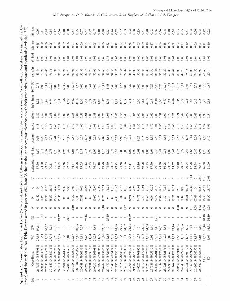
11A

ppen

dix

A. C

oord

inat

es, l

and

use a

nd co

ver (

WS=

woo

dlan

d sa

vann

a; G

W=

gras

sy-w

oody

sava

nna;

PS=

par

klan

d sa

vann

a; W

= w

etla

nd; P

=pas

ture

; A=

agric

ultu

re; U

= ur

ban)

and

site

var

iabl

es (s

ee T

able

1) r

epre

sent

ed in

per

cent

(%) f

rom

38

sites

in th

e up

per A

ragu

ari r

iver

bas

in w

ith th

eir r

espe

ctiv

e m

eans

and

stan

dard

s dev

iatio

n (S

D).

Site

sC

oord

inat

esW

SG

WPS

W

PA

Uxc

denm

idw

1_ha

llsd

dept

hxw

xd

xslo

pe

lsub

_dm

m

PCT_

FN

pct_

sfgf

xf

c_lw

d xf

c_br

s xf

c_na

t 1

2671

33 S

/ 785

7898

E27

,95

59,6

30

012

,42

00

87,3

01,

509,

580,

880,

871,

3212

,73

43,6

40,

040,

350,

792

2906

34 S

/ 787

4629

E11

,54

081

,54

02,

394,

540

74,2

00,

1429

,56

2,70

0,69

0,78

0,00

70,9

10,

000,

000,

113

2670

52 S

/ 787

1871

E19

,55

10,7

70

015

,84

53,8

40

92,6

50,

5819

,84

1,30

1,93

0,96

10,9

160

,00

0,00

0,00

0,34

430

1543

S/ 7

8487

16 E

27,7

48,

240

038

,59

25,4

30

90,1

10,

7310

,76

0,38

2,51

-0,7

427

,27

76,3

60,

010,

050,

145

2219

19 S

/ 785

2625

E8,

2621

,51

00

15,5

554

,68

085

,03

1,20

8,41

0,45

1,09

0,79

0,00

50,9

10,

000,

070,

176

2846

13 S

/ 787

9607

E10

,58

057

,57

012

,52

19,3

30

73,9

30,

0024

,36

2,31

1,29

0,45

1,82

76,3

60,

000,

090,

267

3028

81 S

/ 789

6183

E9,

380

00

090

,62

083

,56

1,93

15,3

20,

761,

02-1

,36

69,0

990

,91

0,00

0,09

0,10

828

6107

S/ 7

8838

67 E

5,84

088

,31

00

5,85

082

,62

0,48

25,8

71,

270,

971,

570,

0032

,73

0,01

0,06

0,50

926

3088

S/ 7

8633

52 E

20,8

70

02,

1671

,32

5,65

064

,57

1,65

17,9

60,

492,

33-0

,02

36,3

669

,09

0,03

0,07

0,37

1028

0748

S/7

8856

69 E

12,6

810

,96

00

5,08

71,2

80

90,7

80,

7417

,20

1,54

0,84

-0,1

414

,55

87,2

70,

010,

150,

2511

2600

81 S

/ 790

0788

E36

,81

5,37

00

57,8

20,

000

79,5

51,

1716

,29

1,00

0,58

1,56

0,00

30,9

10,

010,

060,

5712

2858

92 S

/ 787

5125

E8,

860

69,1

80

021

,96

071

,12

0,73

31,7

81,

441,

010,

930,

0052

,73

0,00

0,04

0,37

1327

7131

S/ 7

8639

15 E

24,3

40

00

075

,66

092

,25

0,98

6,07

0,43

0,89

0,39

3,64

72,7

30,

000,

030,

2714

2407

30 S

/ 782

6308

E23

,35

3,66

00

19,9

253

,07

076

,07

1,07

17,3

31,

011,

450,

760,

0070

,91

0,05

0,05

0,47

1527

4627

S/ 7

9106

05 E

14,1

90

00

22,7

463

,07

091

,18

1,83

17,9

50,

931,

021,

6816

,36

23,6

40,

020,

010,

1016

2509

49 S

/ 789

5246

E21

,86

22,0

80

1,10

33,2

521

,71

048

,80

1,16

8,99

0,30

1,76

-1,0

730

,91

83,6

40,

000,

000,

3017

2914

79 S

/ 787

2603

E18

,65

025

,10

00

56,2

60

98,8

01,

2015

,61

0,35

1,98

1,76

5,45

43,6

40,

180,

320,

6318

2827

45 S

/ 790

5174

E12

,27

00

00

87,7

30

83,0

20,

739,

780,

880,

280,

315,

4594

,55

0,00

0,07

0,44

1926

2337

S/ 7

8936

10 E

14,2

434

,99

00

6,35

44,4

20

87,8

30,

3622

,37

1,14

1,47

1,68

0,00

54,5

50,

050,

330,

5820

3076

15 S

/ 785

4332

E9,

3529

,73

00

1,36

59,5

60

93,5

80,

008,

940,

540,

58-0

,77

14,5

576

,36

0,03

0,22

0,62

2123

5817

S/ 7

8677

97 E

3,11

14,3

20

1,47

081

,10

085

,56

0,00

15,9

81,

040,

451,

380,

0029

,09

0,00

0,04

0,33

2230

8006

S/ 7

8846

30 E

19,4

524

,58

16,5

90

30,9

18,

470

87,1

71,

0910

,32

0,24

1,14

0,74

7,27

43,6

40,

030,

881,

0223

2193

82 S

/ 785

7079

E16

,98

8,79

00

23,2

650

,96

077

,01

1,99

13,7

00,

811,

050,

929,

0949

,09

0,03

0,09

0,68

2424

6327

S/ 7

8701

63 E

11,2

70

00

34,7

254

,01

085

,16

0,61

9,27

0,37

0,66

0,00

0,00

90,9

10,

000,

050,

1325

3069

19 S

/ 784

7966

E19

,13

25,0

30

08,

8347

,01

086

,76

0,00

9,18

0,45

0,66

0,63

3,64

63,6

40,

000,

090,

5126

3078

23 S

/ 786

2520

E13

,28

14,5

00

012

,63

59,5

90

86,2

31,

8614

,08

1,52

0,60

-0,1

59,

0989

,09

0,05

0,18

0,48

2727

7088

S/ 7

9053

15 E

7,92

1,86

00

0,00

90,2

20

87,3

01,

6411

,85

0,75

0,65

0,69

7,27

56,3

60,

010,

170,

4228

2980

89 S

/ 789

0130

E17

,37

2,08

45,6

10

32,7

72,

160

79,8

12,

3517

,96

1,01

0,83

-0,8

854

,55

100,

000,

000,

010,

5629

3034

58 S

/ 785

2641

E12

,61

26,4

10

012

,09

48,8

90

85,7

00,

4114

,33

0,95

0,31

0,00

7,27

87,2

70,

000,

060,

6630

2833

25 S

/ 785

2176

E11

,33

8,01

00

3,13

77,5

30

56,2

80,

3316

,03

2,34

1,07

-0,6

336

,36

87,2

70,

050,

180,

4831

2289

95 S

/ 786

6812

E7,

080

00

4,62

88,3

00

93,3

21,

886,

180,

310,

780,

6310

,91

60,0

00,

000,

050,

4832

2911

68 S

/ 783

8651

E15

,02

12,3

00

015

,85

56,8

30

75,2

70,

6716

,33

1,00

0,85

-0,0

914

,55

69,0

90,

010,

080,

5433

2408

34 S

/ 785

7101

E4,

5610

,34

04,

404,

9875

,72

038

,10

1,75

22,5

32,

130,

21-1

,05

52,7

389

,09

0,00

0,02

0,23

3427

4040

S/ 7

8722

32 E

33,2

157

,56

00

8,46

0,78

088

,37

0,27

10,4

00,

500,

490,

3710

,91

47,2

70,

000,

220,

8535

2750

81 S

/ 787

0412

E14

,77

5,19

00

18,3

161

,73

090

,24

0,47

11,7

60,

470,

990,

225,

4578

,18

0,01

0,10

0,31

3629

7969

S/ 7

8321

65 E

10,0

16,

410

3,31

21,1

742

,68

16,4

117

,78

4,63

10,0

40,

680,

830,

6810

,91

60,0

00,

000,

030,

0437

2631

65 S

/ 786

4557

E28

,97

00

3,54

67,4

90

028

,74

3,45

12,3

40,

460,

470,

4212

,73

74,5

50,

040,

060,

5038

2348

47 S

/ 786

2538

E6,

639,

000

4,62

15,5

261

,64

2,60

6,55

3,91

12,1

80,

710,

640,

753,

6460

,00

0,00

0,05

0,45

M

ean

15,5

511

,40

10,1

00,

5416

,58

45,3

20,

5076

,38

1,20

14,9

60,

940,

980,

4113

,30

65,6

90,

020,

120,

42

SD8,

0714

,92

24,1

91,

2818

,37

29,7

52,

6821

,50

1,06

6,15

0,61

0,54

0,83

16,6

920

,14

0,03

0,16

0,22

Documents

Influence of environmental variables on stream fish fauna