Embed Size (px)
Citation preview

Influence of biological activity on
morphology and bed composition
in the Friesche Zeegat
M.Sc. Thesis
Jeroen A. de Koning
Enschede, December 2005
Committee:
dr. ir. D.C.M. Augustijn
dr. ir. M.A.F. Knaapen
drs. M.B. de Vries
University of Twente
Faculty of Engineering Technology
Department for Water Engineering and Management

Preface
This report forms the completion of my study Civil Engineering & Manage-ment at the Department for Water Engineering and Management, which ispart of the Faculty of Engineering Technology at the University of Twente,The Netherlands. I would like to thank the members of my graduationcommittee dr. ir. Denie Augustijn and dr. ir. Michiel Knaapen from theUniversity of Twente and drs. Mindert de Vries from WL|Delft Hydraulicsfor their support and supervision. I would also like to thank Gerben de Boerfor his help with Delft3D.
Special thanks goes to Dominic, Meinard, Corne, Bas, Wil, Steven, Al-fred and Tessa for the ’energy’ and ’motivation’ boosts they gave me, eachtime one of them graduated. And of course for the endless discussions andfun during coffee breaks or at the barbecue/swimming pool parties.
Marco, Jeffrey and Bartje, thanks for listening to me during those end-less ’discussions’ in the Vestingbar. Finally, I would like to thank my parentsfor supporting me (not only financially), my brothers Michiel and Sander andmy sister Hilde. But most of all I would like to thank my girlfriend Annemiek,for supporting me especially in the last few weeks.
Jeroen de KoningEnschede, December 2005
i


Abstract
There is an increasing interest between abiotic and biotic environments of rivers, lakes, es-tuaries and seas. In the Wadden Sea, biological activity can have a considerable influenceon changes in bed level and composition. For example, Macoma balthica redistributes anddestabilises the bed by motion through the bottom. Diatoms stabilise the bed by forming asticky substances which glues the sediment together. Mussel bed increase the roughness ofthe bed and by filtrating the water column, they increase the deposition of faeces betweentheir shells. Apart from natural hazards to biology, like cold winters and storms, there isa huge scala of human interests, which can influence biology. There are industrial interestslike gas and sand mining, and fishery, or recreational interests, like mud pounding (in Dutch:wadlopen), and water sports.
Especially, the industrial activities have the largest impact on biology. Sand mining hasa large impact on local bed levels and may have an impact on species abundance, e.g. settle-ment of mussel larvae and existence of Macoma balthica. Gas mining results in a large-scalebed level decrease, which can influence the height of the mussel beds, or result in a decreaseof the Chlorophyll-a concentration, because of the lack of light they need for photosynthesis.Fishery directly influences species abundance, but an unwanted side effect is the dragging ofthe fishing nets over the bottom. This also negatively influences biology living in, near or onthe bottom.
In this report the influence of biological activity on morphology and composition in theFriesche Zeegat, a tidal inlet in the Dutch Wadden Sea, is discussed. Van Ledden (2003) de-veloped an application to the Friesche Zeegat of the sand-mud model, based on the numericalmodel Delft3D. This sand-mud model is extended with the biological parameters proposedin Paarlberg et al. (2005), in order to simulate the influence of the bivalve Macoma balthica,diatoms and mussel beds. In Paarlberg et al. (2005), a description is given of the destabilis-ing and stabilising effect of Macoma balthica and diatoms on the critical bed shear stress anderosion coefficient.
Macoma balthica (individuals/m2) decreases the critical bed shear stress and increases theerosion coefficient, while diatoms (Chlorophyll-a content, µg/g) increase the critical bed shearstress and decrease the erosion coefficient. This is also applied to the stabilising effect thatthe mussel beds have on the bed surface. The mussel beds are parameterised as a constantChlorophyll-a content with a maximum stabilising effect. A reference situation is developed inorder to compare the influence of the different organisms on changes in bed level and composi-tion. Both, the results from the reference situation and the results including biological activity,are compared with observed data from the morphological development of the Friesche Zeegat.
iii

Comparing the reference situation with observed data indicate that the mud content in thetop layer of the bottom and the bed level change show similarities and differences. Thecomputed mud content is too high in the entire basin, but the mud distribution shows goodagreement. The bed level change shows good agreement in the entrance of both tidal chan-nels. In the tidal basin net erosion is observed, but the model predicts a slight sedimentation.The magnitude of erosion and sedimentation is not of the same order. The observed datais obtained from a period of 25 years, while the computed data is based on a period of 2 years.
The results including biological activity show better agreement with the observed mud contentand bed level change. The destabilising effect by the bivalve Macoma balthica is dominantover the stabilising effect caused by the diatoms or mussel beds. However, because of an errorin the model, the contribution of the stabilising effect by the mussel beds on the mud contentand bed level change is not very reliable. In order to diminish the unwanted influence of themussel beds, also a simulation without the mussel beds is performed. These results show thatthe stabilising effect by the mussel beds have a significant influence on the mud distributionbut not on the total amount of mud. The influence of the mussel beds can not be neglected,but the destabilising effect is more significant than the stabilising. So, the total amount ofmud decreases significant by the influence of biological activity.
For further research it is necessary to implement the biological parameters in the new versionof the sand-mud model. In order to study the influence of the waves on the bed shear stressand to increase the simulation period to a greater time-scale. It is recommended to imple-ment the seasonal influence on species abundance and existence and the interaction betweenorganisms.
iv

Contents
Preface i
Abstract iii
List of Figures vii
List of Tables ix
1 Introduction 1
1.1 Biogeomorphology . . . . . . . . . . . . . . . . . . . . . . . . . . . . . . . . . 1
1.2 Area description . . . . . . . . . . . . . . . . . . . . . . . . . . . . . . . . . . 2
1.3 Sand-mud model . . . . . . . . . . . . . . . . . . . . . . . . . . . . . . . . . . 3
1.4 Research objective . . . . . . . . . . . . . . . . . . . . . . . . . . . . . . . . . 4
1.5 Outline of the report . . . . . . . . . . . . . . . . . . . . . . . . . . . . . . . . 5
2 Biological characteristics 7
2.1 Macoma Balthica . . . . . . . . . . . . . . . . . . . . . . . . . . . . . . . . . . 7
2.2 Diatoms . . . . . . . . . . . . . . . . . . . . . . . . . . . . . . . . . . . . . . . 9
2.3 Mussel beds . . . . . . . . . . . . . . . . . . . . . . . . . . . . . . . . . . . . . 10
3 Morphological and biological interaction 13
3.1 Sand-mud model description . . . . . . . . . . . . . . . . . . . . . . . . . . . . 13
3.2 Parameterisation of biological activity . . . . . . . . . . . . . . . . . . . . . . 15
3.3 Sand-mud-bio model . . . . . . . . . . . . . . . . . . . . . . . . . . . . . . . . 18
4 Model set-up of the reference situation 19
4.1 Simulation of the model . . . . . . . . . . . . . . . . . . . . . . . . . . . . . . 19
4.2 Computational grid and bathymetry . . . . . . . . . . . . . . . . . . . . . . . 20
4.3 Boundary conditions . . . . . . . . . . . . . . . . . . . . . . . . . . . . . . . . 20
4.4 Initial conditions . . . . . . . . . . . . . . . . . . . . . . . . . . . . . . . . . . 23
5 Reference situation 25
5.1 Water level and tidal currents . . . . . . . . . . . . . . . . . . . . . . . . . . . 26
5.2 Bed shear stress . . . . . . . . . . . . . . . . . . . . . . . . . . . . . . . . . . . 28
5.3 Suspended sediment . . . . . . . . . . . . . . . . . . . . . . . . . . . . . . . . 30
5.4 Mud content . . . . . . . . . . . . . . . . . . . . . . . . . . . . . . . . . . . . 33
5.5 Bed level change . . . . . . . . . . . . . . . . . . . . . . . . . . . . . . . . . . 35
v

5.6 Conclusion . . . . . . . . . . . . . . . . . . . . . . . . . . . . . . . . . . . . . 35
6 Influence biological activity 37
6.1 Bed shear stress . . . . . . . . . . . . . . . . . . . . . . . . . . . . . . . . . . . 376.2 Erosion coefficient . . . . . . . . . . . . . . . . . . . . . . . . . . . . . . . . . 396.3 Mud content . . . . . . . . . . . . . . . . . . . . . . . . . . . . . . . . . . . . 396.4 Bed level change . . . . . . . . . . . . . . . . . . . . . . . . . . . . . . . . . . 436.5 Conclusion . . . . . . . . . . . . . . . . . . . . . . . . . . . . . . . . . . . . . 45
7 Discussion 47
7.1 Sand-mud-bio model . . . . . . . . . . . . . . . . . . . . . . . . . . . . . . . . 477.2 Biological characteristics . . . . . . . . . . . . . . . . . . . . . . . . . . . . . . 49
8 Conclusions & Recommendations 51
8.1 Conclusions . . . . . . . . . . . . . . . . . . . . . . . . . . . . . . . . . . . . . 518.2 Recommendations . . . . . . . . . . . . . . . . . . . . . . . . . . . . . . . . . 53
Bibliography 55
vi

List of Figures
1.1 The influences of the biological processes on the morphological cycle (De Vries,2005). . . . . . . . . . . . . . . . . . . . . . . . . . . . . . . . . . . . . . . . . 2
1.2 Location of the Friesche Zeegat (Van Leeuwen et al., 2003). . . . . . . . . . . 3
1.3 Setup of the original sand-mud model (Van Ledden, 2003). . . . . . . . . . . 4
2.1 The bivalve Macoma balthica . . . . . . . . . . . . . . . . . . . . . . . . . . . 7
2.2 Macoma balthica (a) biomass (gC/m2) (Wijsman, 2004) and (b) distribution(ind/m2) according to the four depth zones in the Friesche Zeegat. . . . . . . 8
2.3 Chlorophyll-a (µgChl/g) (a) concentration in one meter water depth and (b)distribution in the Friesche Zeegat according to the depth zones. . . . . . . . 10
2.4 Mytilus edulis (directly from the website: http://www.weichtiere.at). . . . . . 11
2.5 Schematisation of the mussel beds in the Friesche Zeegat. . . . . . . . . . . . 12
3.1 The effect of (a) Macoma balthica density on the destabilisation factor (fd(B))and (b) Chlorophyll-a content on the stabilisation factor (fs(C)) for the criticalbed shear stress. . . . . . . . . . . . . . . . . . . . . . . . . . . . . . . . . . . 16
3.2 The effect of (a) Macoma balthica density on the destabilisation factor (gd(B))and (b) Chlorophyll-a content on the stabilisation factor (gs(C)) for the erosioncoefficient. . . . . . . . . . . . . . . . . . . . . . . . . . . . . . . . . . . . . . . 17
3.3 Set-up of the original sand-mud model included with influence of the biologicalactivity (Paarlberg et al., 2005). . . . . . . . . . . . . . . . . . . . . . . . . . 18
4.1 Numerical grid (X,Y) and depth contours (m) of the Friesche Zeegat. The openboundaries are situated in the North Sea, the basin is surrounded by closedboundaries in the east, south and west. . . . . . . . . . . . . . . . . . . . . . . 20
4.2 Wave heights (m) during (a) maximum ebb currents and (b) low water. . . . 21
4.3 Wave heights (m) during (a) maximum flood currents and (b) high water. . . 22
5.1 Observation points and depth contours (m) in the Friesche Zeegat accordingto Mean Sea Level. . . . . . . . . . . . . . . . . . . . . . . . . . . . . . . . . . 25
5.2 Water level during a single tidal period at location: (a) 1 - 4, Pinkegat andPinkegat Noord and (b) 5 - 8, Nieuwe Westgat and Roode Hoofd. . . . . . . . 26
5.3 Current velocities (m/s) during a tidal period at location: (a) 1 - 4, Pinkegatand Pinkegat Noord and (b) 5 - 8, Nieuwe Westgat and Roode Hoofd. . . . . 27
vii

5.4 Tidal current velocities (m/s) in the Friesche Zeegat: (a) maximum ebb, (b)maximum flood currents and (c) difference between the maximum ebb andflood currents (positive value indicates higher flood current velocities, negativevalue indicates higher ebb current velocity). . . . . . . . . . . . . . . . . . . . 28
5.5 Bed shear stress (N/m2) during a tidal period at location: (a) 1 - 4 and Pinkegat(Noord) and (b) 5 - 8, Nieuwe Westgat and Roode Hoofd. The horizontal linesrepresent the critical bed shear stress for non-cohesive mixtures (τcr,nc) and forcohesive mixtures (τcr,c). . . . . . . . . . . . . . . . . . . . . . . . . . . . . . . 29
5.6 Suspended mud concentration (g/l) profiles during a tidal period in: (a) lo-cation 1 - 4 and Pinkegat and (b) location 5 - 8, Nieuwe Westgat and RoodeHoofd. . . . . . . . . . . . . . . . . . . . . . . . . . . . . . . . . . . . . . . . . 30
5.7 Observed suspended sediment concentration (g/l) at (a) Nieuwe Westgat and(b) Roode Hoofd from 1973 - 2003 (http://www.waterbase.nl). The horizontallines represent the average concentration during that period. . . . . . . . . . 32
5.8 Observed mud content in the Friesche Zeegat (Van Rijsewijk, 2002). . . . . . 325.9 Mud content (%) after (a) 1 year and (b) 2 years. . . . . . . . . . . . . . . . . 335.10 Mud content (%) after (a) 4 year and (b) 8 years. . . . . . . . . . . . . . . . . 335.11 Computed net sedimentation of mud (ton) in the Friesche Zeegat. . . . . . . . 345.12 Bed level change (m) after: (a) 1 year (b) 2 years. . . . . . . . . . . . . . . . 345.13 Observed bed level change in the ebb-tidal delta and in the tidal basin of the
Zoutkamperlaag (Van Ledden, 2003). . . . . . . . . . . . . . . . . . . . . . . . 36
6.1 Destabilising effect caused by the M. balthica: (a) mud content (%) in the toplayer of the bed and (b) difference in mud content (%). ’+’ denotes areas wherethe mud content increases and ’-’ denotes a decrease of the mud content as aresult from the influence of biology. . . . . . . . . . . . . . . . . . . . . . . . . 40
6.2 Stabilising effect caused by algae: (a) mud content (%) in the top layer of thebed and (b) difference in mud content (%). ’+’ denotes areas where the mudcontent increases and ’-’ denotes a decrease of the mud content as a result fromthe influence of biology. . . . . . . . . . . . . . . . . . . . . . . . . . . . . . . 40
6.3 Stabilising effect caused by mussel beds: (a) mud content (%) in the top layerof the bed and (b) difference in mud content (%). ’+’ denotes areas where themud content increases and ’-’ denotes a decrease of the mud content as a resultfrom the influence of biology. The contours represent the mussel beds. . . . . 41
6.4 Combination of (de)stabilising effect caused by all organisms: (a) mud content(%) in the top layer of the bed and (b) difference in mud content (%). ’+’denotes areas where the mud content increases and ’-’ denotes a decrease ofthe mud content as a result from the influence of biology. . . . . . . . . . . . 42
6.5 Difference in bed level (m) as a result of (a) the destabilising effect causedby M. balthica and (b) the stabilising effect caused by algae compared to thereference situation. . . . . . . . . . . . . . . . . . . . . . . . . . . . . . . . . . 43
6.6 Difference in bed level (m) as a result of (a) the stabilising effect of the musselbeds and (b) the combination of (de)stabilising effect caused by all organismscompared to reference situation. . . . . . . . . . . . . . . . . . . . . . . . . . 44
6.7 Bed level change (m) as a result of the influence of biological activity. . . . . 44
viii

List of Tables
2.1 Depth zones (Mean Sea Level) and yearly average biomass (gC/m3 and density(ind/m2) of M. balthica . . . . . . . . . . . . . . . . . . . . . . . . . . . . . . 9
2.2 Depth zones (Mean Sea Level) and yearly average biomass of diatoms. . . . . 9
4.1 Water level amplitudes at Wierumergronden, Huibertgat, Western and Easternmodel boundary (Van Ledden, 2003). . . . . . . . . . . . . . . . . . . . . . . . 21
4.2 Settings of the physical parameters of the reference computation. . . . . . . . 22
5.1 Percentage in time exceeding τnc and τc during one tidal period for each ob-servation point. . . . . . . . . . . . . . . . . . . . . . . . . . . . . . . . . . . . 29
5.2 Average suspended mud concentration (g/l) during the ebb and flood period. 315.3 Observed and computed average and maximum suspended mud concentrations
for location Nieuwe Westgat and Roode Hoofd. . . . . . . . . . . . . . . . . . 31
6.1 Observation points with corresponding correction factor for the critical bedshear stress (Bτ = fd(B) · fs(C)) [-] and corrected critical bed shear stress[N/m2] for each scenario. . . . . . . . . . . . . . . . . . . . . . . . . . . . . . . 38
6.2 Percentage in time exceeding the critical bed shear stress in the non-cohesive(τc) and cohesive regime and (τc) for each observation point and scenario. . . 38
6.3 Observation points with corresponding correction factor for the erosion rate(Be = gd(B) · gs(C)) [-]. . . . . . . . . . . . . . . . . . . . . . . . . . . . . . . 39
6.4 Estimation of the total amount of mud remaining in the Friesche Zeegat after2 years and average amount during a tidal period. . . . . . . . . . . . . . . . 42
ix


Chapter 1
Introduction
1.1 Biogeomorphology
There is an increasing interest in the interaction between the abiotic and biotic environmentsof rivers, lakes, estuaries and seas. Biogeomorphology is the interaction between biologyand morphology. Morphology is the interaction between water and sediment motion andbed topography. Biology is the study of the relationships between organisms and their en-vironment. Biological activity affects the sediment structure and sediment dynamics and itmay influence the hydrodynamics. For example, a juvenile mussel bed collects considerableamounts of fine sediments between August and November, and beds can rise up to 30-40 cmabove the surrounding mudflats (Dankers et al., 2001).
Benthic organisms have an effect on their environment by stabilising or destabilising the sur-face of the bed. The term benthos refers to all organisms living in, on or near the bottom.Different types of benthos can be distinguished: zoobenthos, like clams, mussels and worms,and phytobenthos, like algae. Deposit feeders like the bivalve Macoma batlhica and the laverspire shell (Hydrobia ulvae) feed on organic matter in or on the sediment surface. By burrow-ing and motion through the bed these organisms redistribute the bed and cause resuspensionof the sediment. This bioturbation results in a less consolidated bed and lower critical bedshear stress. In figure 1.1 a schematisation is given of the effects that the different benthoshave on the morphological cycle.
The excretion of mucus or EPS (Extracellular Polymeric Substance) by algae glues the sed-iment together, this results in an increase of the critical bed shear stress. Algal-mats areformed when large biomasses of diatoms occur, e.g. during calm springs and summers. Thesediatoms populations strongly fluctuate as a result of changes in environmental conditions.Mussel bed also have a stabilising effect, they protect the bed surface from resuspension anderosion. They even enhance the flux of suspended sediment to the bed via suspension feedingand biodeposition. Suspension feeding means that the organisms filtrate water out of thewater column to obtain food. During this process also fine-grained sediments are filtered outof the water. The faeces and pseudofeaces these mussels excrete, remain between the shellsand their bysus threads, this causes biodeposition (Widdows and Brinsley, 2002).

2 Chapter 1. Introduction
Sediment transport
Critical bed shear stress
Bed composition
Bed level
Flow & waves
Erosion rate
Stabilisation (Re)suspension Deposition Roughness
Destabilisation Redistribution of
the bed
-
+
-
+
Algae/ Diatoms
Mytilus edulis
+
+
-
+
Macoma balthica/
Hydrobia ulvae
+
+ +
+
-
Figure 1.1: The influences of the biological processes on the morphological cycle (De Vries, 2005).
In the past few years several studies have been conducted on the before mentioned biologicalinfluences on the large-scale morphology. Oost (1995) examined the influence of biodepo-sition by Mytilus edulis (the blue mussel) in the Dutch Wadden Sea. He states that highamounts of faeces and pseudo-faeces, which are produced by mussels, influence the suspendedsedimentation concentration in the water column and sedimentation of fine-grained sediments.
Knaapen et al. (2003) focussed on the effects of bioturbation and biostabilisation and thepossibility to introduce these biological effects directly into long-term morphodynamic models.This idea has been applied to two cases. The results of the first case indicate that this approachcan reproduce the influence of benthic organisms on the mud content of the bed. The secondcase shows that even low numbers of organisms can influence the characteristics of large bedforms. Paarlberg et al. (2005) studied the effects of biodestabilisers and biostabilisers on theerosion and mixing process of the sediment bed on an intertidal flat in the Western Scheldt,the Netherlands. The destabilising organisms always cause a significant decrease in mudcontent in the bed and an increase of erosion, while the stabilising organisms can increase themud content in the bed and sedimentation.
Because the bivalve Macoma balthica and diatoms are representatives of organisms with adestabilising effect and a stabilising effect (Widdows et al., 1998; Widdows and Brinsley, 2002),these organisms are implemented in the sand-mud model by Van Ledden (2003). Furthermorein this research, a third organism is added which causes a stabilising effect on the sedimentstrength. Also, mussel beds can have a significant influence on sedimentation in the FriescheZeegat (Oost, 1995).
1.2 Area description
The Dutch Wadden Sea is a shallow, semi-enclosed part of the North Sea, mainly consisting oftidal mud flats, sand flats, gullies and salt marshes. The area is bordered by a series of barrierislands, the Wadden Islands. The Wadden Sea stretches along the North Sea coast from Den
1.3 Sand-mud model 3
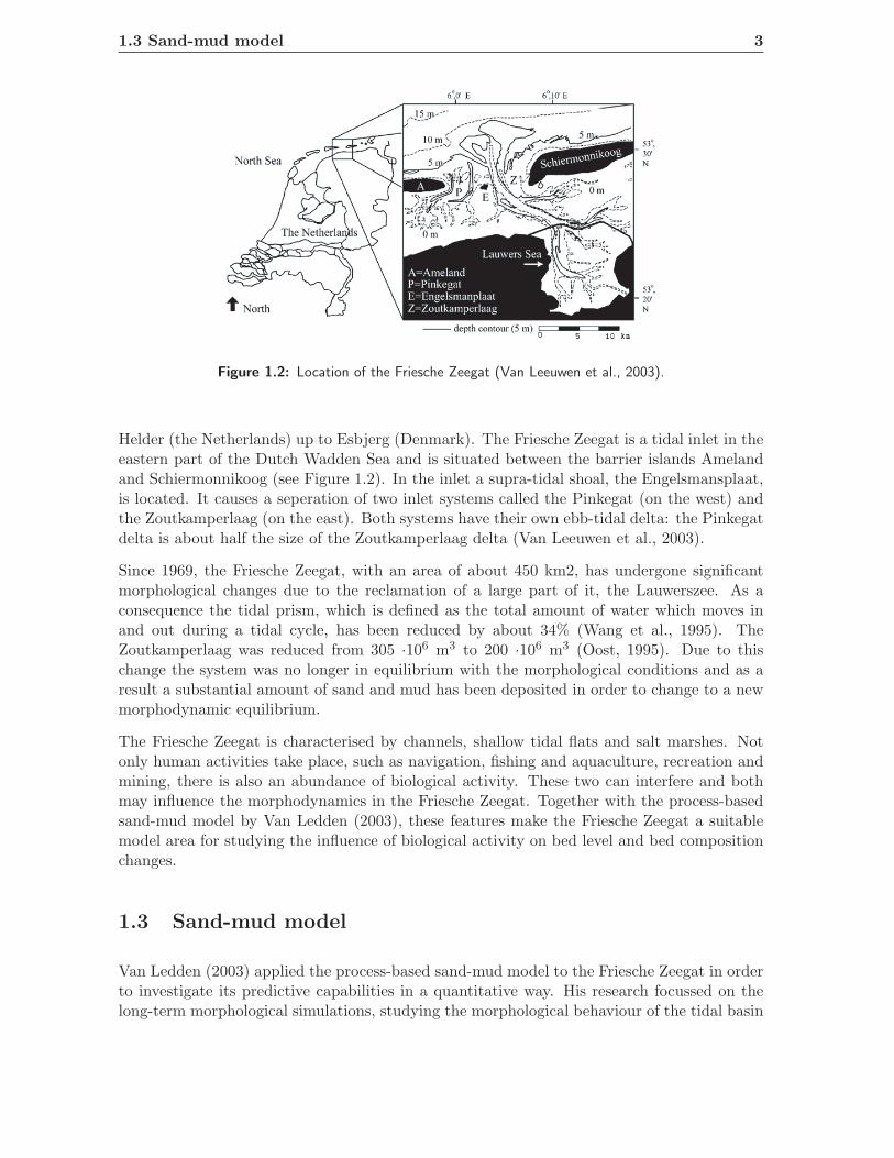
Figure 1.2: Location of the Friesche Zeegat (Van Leeuwen et al., 2003).
Helder (the Netherlands) up to Esbjerg (Denmark). The Friesche Zeegat is a tidal inlet in theeastern part of the Dutch Wadden Sea and is situated between the barrier islands Amelandand Schiermonnikoog (see Figure 1.2). In the inlet a supra-tidal shoal, the Engelsmansplaat,is located. It causes a seperation of two inlet systems called the Pinkegat (on the west) andthe Zoutkamperlaag (on the east). Both systems have their own ebb-tidal delta: the Pinkegatdelta is about half the size of the Zoutkamperlaag delta (Van Leeuwen et al., 2003).
Since 1969, the Friesche Zeegat, with an area of about 450 km2, has undergone significantmorphological changes due to the reclamation of a large part of it, the Lauwerszee. As aconsequence the tidal prism, which is defined as the total amount of water which moves inand out during a tidal cycle, has been reduced by about 34% (Wang et al., 1995). TheZoutkamperlaag was reduced from 305 ·106 m3 to 200 ·106 m3 (Oost, 1995). Due to thischange the system was no longer in equilibrium with the morphological conditions and as aresult a substantial amount of sand and mud has been deposited in order to change to a newmorphodynamic equilibrium.
The Friesche Zeegat is characterised by channels, shallow tidal flats and salt marshes. Notonly human activities take place, such as navigation, fishing and aquaculture, recreation andmining, there is also an abundance of biological activity. These two can interfere and bothmay influence the morphodynamics in the Friesche Zeegat. Together with the process-basedsand-mud model by Van Ledden (2003), these features make the Friesche Zeegat a suitablemodel area for studying the influence of biological activity on bed level and bed compositionchanges.
1.3 Sand-mud model
Van Ledden (2003) applied the process-based sand-mud model to the Friesche Zeegat in orderto investigate its predictive capabilities in a quantitative way. His research focussed on thelong-term morphological simulations, studying the morphological behaviour of the tidal basin

4 Chapter 1. Introduction
Sand transport Mud transport
Flow
Bed level
Bed composition
Figure 1.3: Setup of the original sand-mud model (Van Ledden, 2003).
after the closure of it in 1969.
The sand-mud model is 1DV (point) model which gives a prediction of the bed compositionin a particular point. It is coupled with the numerical modelling system Delft3D (D3D) byapplying it to the whole grid. This makes it possible to perform morphological calculationsin order to predict the spatial distribution of sand and mud in the Friesche Zeegat. D3Dis suited for hydrodynamic and morphodynamic computations for coastal, rivers and estu-arine environments. It can carry out simulations of flow, sediment transport, morphologicaldevelopment and waves. WL|Delft Hydraulics is copyright owner of the Software.
The sand-mud model is chosen because it focusses not on sand transport only, but also on thefine-grained sediment transport. Most organisms are believed to influence the mud contentin the bottom and mud concentration in the water column (Knaapen et al., 2003; Paarlberget al., 2005).
1.4 Research objective
This research aims at contributing to the understanding and modelling of biological influenceson large-scale morphological changes in estuaries and tidal basins. The objective is:
To determine the influence of biology on bed level and composition in the Friesche Zeegat, byimplementing the stabilising and destabilising effect, that organisms have on the surface ofthe bed, in the existing sand-mud model by Van Ledden (2003).
The research objective implies the following research questions of which the answers willcontribute to the fulfillment of this objective.� Which organisms have affect on the morphology and bed composition in the Friesche
Zeegat?� How can these organisms be implemented in the sand-mud model by Van Ledden (2003)?� What is the difference on morphology and bed composition between simulations withand without biological activity?

1.5 Outline of the report 5� Does the sand-mud-bio model show agreement with actual measurements in the FriescheZeegat?
Biological activity has influence on the stability of the bed in the Friesche Zeegat by affectingthe critical bed shear stress and erosion coefficient (Paarlberg et al., 2005). These parametersare included in the sand-mud model by Van Ledden (2003). The results of the simulationswith and without biological activity are compared with each other and compared with themeasurements of bed composition and computed mud contents in the Friesche Zeegat.
1.5 Outline of the report
Chapter 2 describes which organisms have influence on the sediment strength and their char-acteristics. First the background of the sand-mud model and second the parametrisation ofthe biological influence is studied in Chapter 3. In Chapter 4 the model set-up of the referencesituation without biological activity is described and the results of this reference situation aregiven in Chapter 5. In Chapter 6 the results from the reference situation are compared withthe results from three different scenarios with biological activity. Chapter 7 contains thediscussion of the results of this research, and in Chapter 8 the main conclusions are given,together with recommendations for further research.


Chapter 2
Biological characteristics
In this research the main destabilising organism is the bivalve Macoma balthica. The stabil-ising effect is caused by diatoms and mussel beds. The biological characteristics of the threedifferent organisms are described. M. balthica abundance is schematised in four differentdepth zones. The content of Chlorophyll-a is also depth dependent and the distribution ofthe mussel beds is based on actual data.
2.1 Macoma Balthica
The bivalve, Macoma balthica, is widely abundant throughout north-west Europe. It can bepresent at very high but variable densities and it is found from the upper part of the intertidalflat to the shallow subtidal zone. It is not recorded in parts of the North Sea deeper than25 m. The main breeding period of the M. balthica is between February and May. A secondspawning period occurs in August. Along the Dutch coast the highest biomasses are found inestuaries and tidal inlets. The bivalve prefers muddy sediments with relatively high silt-claypercentages (Holtmann et al., 1996). M. balthica has a long inhalant siphon that enablesit to feed in two different ways; deposit and suspension feeding. The burying depth of thebivalve during autumn and winter is sufficient to protect it from most predators and againstwashing away and extreme low temperatures. The average depth during temperate springand summer in the western Dutch Wadden Sea is between 2 to 3 cm and in the eastern Dutch
Figure 2.1: The bivalve Macoma balthica

8 Chapter 2. Biological characteristics
Wadden Sea it is between 2.5 and 6.5 cm. This is well within reach of the predators (De Goeijand Honkoop, 2002).
Macoma balthica densities are generally higher following a cold winter, this is caused by anincrease in food source and a reduction of predators . There is also a relationship betweenthe M. balthica density, its grazing activity and the microphytobenthos biomass. At times ofhigh M. balthica abundance the microphytobenthos will be grazed and the biomass lowered(Widdows and Brinsley, 2002). Studies in the Humber and the Westerschelde have recordeda correlation between sediment erodibility and the activity and density of M. balthica. As aresult of the burrowing, deposit feeding and grazing activity of M. balthica, the bed surfacehad a lower critical shear stress and a higher erosion coefficient (Widdows et al., 1998).
2.1.1 Macoma balthica density and distribution
M. balthica can be found from the upper part of the intertidal flat to the shallow subtidal zone.For the Western Wadden Sea seasonal variations in biomass data of M. balthica is availablerelated to different depth zones (Wijsman, 2004). The seasonal variations in biomass ispresented in Figure 2.2(a). From this data set the annual average biomass is taken in orderto apply it to the Friesche Zeegat. In ecology M. balthica biomass is an accepted indicator,however, according to Paarlberg et al. (2005) M. balthica density correlates better with criticalbed shear stress and erosion coefficient. The average grazer weight is 0.01 gC/n, this meansthat a biomass of 1 gC/m2 represents 100 individuals/m2 (ind/m2). The number of ind/m2
is divided over four depth zones, which are given in Table 2.1. In zone 1 the average densityis 1078 ind/m2, zone 2 and 3 both have a density of 129 ind/m2. In zone 4 there is no activityof the bivalve M. balthica. In Figure 2.2(b) the four depth zones in the Friesche Zeegat arepresented.
January December0
2
4
6
8
10
12
14
16
Time
Bio
mas
s (g
C/m
2 )
Zone 1Zone 2 and 3
(a)
0 20 40 60 80 1000
10
20
30
40
50
Schiermonnikoog
X (gridcell)
Engels−manplaat
Ameland
Y (
grid
cell)
0 1 2 3 4
(b)
Figure 2.2: Macoma balthica (a) biomass (gC/m2) (Wijsman, 2004) and (b) distribution (ind/m2) ac-cording to the four depth zones in the Friesche Zeegat.

2.2 Diatoms 9
depth zone h (m) biomass (gC/m2) density (n/m2)
1 h ≤ 1 10.78 10782 1 < h ≤ 2 1.29 1293 2 < h ≤ 3 1.29 1294 h > 3 0 0
Table 2.1: Depth zones (Mean Sea Level) and yearly average biomass (gC/m3 and density (ind/m2) ofM. balthica
2.2 Diatoms
Diatoms are restricted to the intertidal or shallow subtidal zone in turbid waters (e.g., estu-aries and coastal lagoons) due to lack of light available for photosynthesis in deeper water.This implies that the stabilising effect brought about by diatoms will mainly be restricted tothe intertidal zone (Andersen et al., 2004). Sutherland et al. (1998) demonstrated a strongrelationship between critical erosion shear stress and microphytobenthos density. This studyshowed a significant increase in critical shear stress and a reduction in erosion rate withincreasing Chlorophyll-a content.
During a bloom period in spring algae mats are formed by large densities of diatoms whichproduce a sticky substance made of polysaccharides that glues the sediment together andprevents it from erosion. These communities include both motile algae (epipelic diatoms) aswell as sessile algae attached to sand grains (epipsammic diatoms) (Wolfstein et al., 2000).
2.2.1 Chlorophyll-a content and distribution
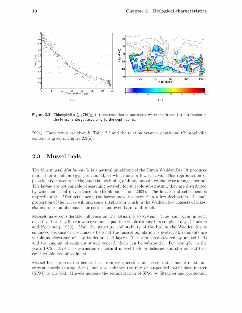
Stabilisation by diatoms is represented by the Chlorophyll- a content [µg g−1], which is anindicator of microphytobenthos biomass (Staats et al., 1998). Because Chlorophyll-a can befound in intertidal or shallow subtidal waters, ten depth zones are used within one meterdepth (mean water level) to give a distribution of the Chlorophyll-a concentration (Blauw,
depth zone h (m) concentration (µgChl/g)
1 0.0 ≤ h < 0.1 34.092 0.1 ≤ h < 0.2 31.983 0.2 ≤ h < 0.3 20.474 0.3 ≤ h < 0.4 16.615 0.4 ≤ h < 0.5 14.106 0.5 ≤ h < 0.6 9.547 0.6 ≤ h < 0.7 6.848 0.7 ≤ h < 0.8 4.349 0.8 ≤ h < 0.9 2.1910 0.9 ≤ h ≤ 1.0 1.18
Table 2.2: Depth zones (Mean Sea Level) and yearly average biomass of diatoms.
10 Chapter 2. Biological characteristics
0 5 10 15 20 25 30 350
0.1
0.2
0.3
0.4
0.5
0.6
0.7
0.8
0.9
1
Chlorophyll−a (µg/g)
Dep
th (
m)
(a)
0 20 40 60 80 1000
10
20
30
40
50
X (gridcell)
Y (
grid
cell)
0 5 10 15 20 25 30 35
(b)
Figure 2.3: Chlorophyll-a (µgChl/g) (a) concentration in one meter water depth and (b) distribution inthe Friesche Zeegat according to the depth zones.
2004). These zones are given in Table 2.2 and the relation between depth and Chlorophyll-acontent is given in Figure 2.3(a).
2.3 Mussel beds
The blue mussel Mytilus edulis is a natural inhabitant of the Dutch Wadden Sea. It producesmore than a million eggs per animal, of which only a few survive. This reproduction ofpelagic larvae occurs in May and the beginning of June, but can extend over a longer period.The larvae are not capable of searching actively for suitable substratum, they are distributedby wind and tidal driven currents (Brinkman et al., 2002). The location of settlement isunpredictable. After settlement, the larvae move no more than a few decimeters. A smallproportion of the larvae will find some substratum which in the Wadden Sea consists of dikes,chains, ropes, adult mussels or cockles and even bare sand or silt.
Mussels have considerable influence on the estuarine ecosystem. They can occur in suchdensities that they filter a water volume equal to a whole estuary in a couple of days (Dankersand Koelemaij, 1989). Also, the structure and stability of the bed in the Wadden Sea isenhanced because of the mussels beds. If the mussel population is destroyed, remnants arevisible as elevations of clay banks or shell layers. The total area covered by mussel bedsand the amount of sediment stored beneath them can be substantial. For example, in theyears 1975 - 1978 the destruction of natural mussel beds by fisheries and storms lead to aconsiderable loss of sediment.
Mussel beds protect the bed surface from resuspension and erosion at times of maximumcurrent speeds (spring tides), but also enhance the flux of suspended particulate matter(SPM) to the bed. Mussels increase the sedimentation of SPM by filtration and production

2.3 Mussel beds 11
Figure 2.4: Mytilus edulis (directly from the website: http://www.weichtiere.at).
of faeces and pseudofaeces around mussel beds. These biodeposits partly settle betweenthe shells of the colony. Resuspension is restricted by the protection of the byssal threads(strong threads which attach the mussel to the bed) and by the shells. In order to remainat the sediment-water interface, the mussels move by using their foot and releasing byssalthreads. The upward movement of the shells creates holes, which are filled with clay and/orsand (Oost, 1995). The sediment underneath the mussel beds is accumulated by biodepositionand physical accretion. This results in an a strong vertical deposition of several dm/year. Ajuvenile mussel bed filtrates considerable amounts of fine silt between August and Novemberand these beds can rise up to 30 - 40 cm above the surroundings. These unstable beds oftendisappear during winter storms. If the bed survives the winter the silt consolidates and formsa stable clay layer. In old mussel beds, the majority of the underlying sediment consists ofsand and clay (Dankers et al., 2001).
The height of the mussel bed is restricted because feeding duration decreases during verticalgrowth. The mussel beds on the intertidal flats of the Wadden Sea normally grow up to meansea level. At higher levels mussels have to spend more energy to withstand the higher waveenergy and longer duration of aerial exposure. Furthermore the vertical growth is limitedbecause of the increased erosion of sediment from the mussel bed (Oost, 1995).
2.3.1 Mussel bed location
According to Brinkman et al. (2002) the presence of mussel beds depends on the wave action,distance to a gully, emersion time and bed composition. A high orbital velocity and flowvelocity would be unfavourable for mussel beds appearance. Washing away of settled musselsand sediment, and the resuspension of sand and silt, negatively affects filtration possibilities.In case of very low flow velocities there is hardly any refreshment of water and thus feedingconditions might turn out to be poor. A large distance of the site to a gully causes lessfavourable feeding conditions for mussels, because a gully serves as a transport route forfood. According to (Brinkman et al., 2002) close to the water line (Mean Sea Level), lessmussel beds appeared and when emersion time was above 50% hardly any mussel bed couldbe found. Very coarse sand or silty environments were not preferred, however the larger partof the Wadden Sea has suitable median grain size conditions.

12 Chapter 2. Biological characteristics
0 20 40 60 80 1000
10
20
30
40
50
X (gridcell)Y
(gr
idce
ll) Ameland Schiermonnikoog
Engels−manplaat
Figure 2.5: Schematisation of the mussel beds in the Friesche Zeegat.
The size of the mussel population in the Dutch Wadden Sea strongly fluctuates from year toyear, as a result of climate-influenced population dynamics and fishery. Mussels can surviveprolonged periods of frost, but the abrasion of mussel beds by moving ice can be catastrophicaccording to Dankers and Koelemaij (1989), as was observed in several winters (1962/’63,1971/’72 and 1984 - 1987). Besides variation in population during several years, seasonaldifferences also influence the amount of biodeposits of mussels. In order to investigate theeffect of seasonal variation on the filtration rate of mussels, Prins et al. (1994) carried outmeasurements of particulate matter uptake by a mussel bed in a concrete tank with a con-tinuous supply of natural seawater from December 1988 till December 1989. Weight loss ofthe mussel occurred during the winter period (December - April) and also between May andJune. The fastest growth rates were observed between April and May and in the period Junetill September. These changes in biomass lead to highly significant differences in clearancerates between months.
In Figure 2.5 a schematisation is shown of the locations of the mussel beds. This data is basedon actual mussel bed locations in spring 2004 (Steenbergen et al., 2004). The total area ofmussel beds at that time was 430 acres. The parametrisation of the mussel bed is modelledin the same way as the diatoms. A constant concentration of 50 µg/g is used to model theeffect on the critical bed shear stress and erosion coefficient by the mussels.

Chapter 3
Morphological and biological
interaction
The application of the sand-mud model to the Friesche Zeegat by Van Ledden (2003) is basedon the numerical modelling system Delft3D. Morphodynamic and hydrodynamic simulationsof coastal, river and estuarine areas are performed in Delft3D.
In this chapter the different modules of the sand-mud model are described, detailed informa-tion about non-cohesive and cohesive sand-mud mixtures can bed found in the PhD-thesisby Van Ledden (2003). Furthermore, an outline of the implementation of the biological char-acteristics is given.
3.1 Sand-mud model description
3.1.1 Flow Module
A crucial parameter for sediment transport processes is the bed shear stress. The bed shearstress is the result of water motion, caused by currents and waves, over the bed and theroughness of the bed itself. Currents are mainly driven by tide, wind, river discharge anddensity differences due to salinity or sediment concentrations. Wind driven waves are locallygenerated or penetrate from the open sea into the estuary or tidal basin.
The three-dimensional behaviour of currents is described by a mass balance equation andthree momentum equations (Van Rijn, 1993). Two important assumptions are made. Thevertical accelerations are small compared to the gravitational acceleration and the densityvariations are small with respect to the water density itself and are only maintained in thegravity term (i.e. ’shallow water’ and ’Boussinesq’ approximation). The remaining dependentvariables in the mass balance and momentum equations are the water level (ζ) and the threevelocity components (u, v, w). By solving these equations the currents induced by tide, shortwaves, river discharge, wind and earth rotation can be modelled.

14 Chapter 3. Morphological and biological interaction
3.1.2 Sediment transport module
The sand transport can be divided into bed load and suspended load transport. Bed loadoccurs near the bed surface and is affected by the flow conditions, while suspended loadis also determined by the upstream conditions. Sediment erosion occurs once the criticalerosion shear stress exerted by moving fluids is exceeded. The critical erosion shear stressis an important parameter in sediment transport mechanics. Below this value little or noerosion occurs, whereas once exceeded significant erosion occurs.
An important distinction in erosional behaviour is made between non-cohesive and cohesivesediment beds. In the non-cohesive regime a sediment bed has a granular structure and doesnot form a coherent mass. The particle size and weight are the most important parameters forerosion. Whereas, cohesive beds form a coherent mass because of electrochemical reactionsbetween the sediment particles. These reactions dominate the erosional behaviour and notparticle size and weight. The transition between non-cohesive and cohesive beds is determinedby the clay (d50 ≤0.002 mm) content.
In the sand-mud model a non-cohesive and cohesive regime is applied. The erosion behaviourof the sediment mixture is considered non-cohesive if the mud content is lower than the criticalmud content (pm,cr) or it is considered cohesive if the mud content exceeds the critical mudcontent.
The exchanges of sediment between the bed and the water column depend on the bed com-position at the bed surface. In Delft3D, the bed load sand transport rate is calculatedafter (Van Rijn, 1993). The net vertical fluxes of suspended sand (Fs) and mud (Fm) nearthe bed are as follows (Van Ledden and Wang, 2001):Non-cohesive regime (pm ≤ pm,cr):
Fs = ws(ca − cs) (3.1)
and
Fm = pmM(n)c
(
τb
τ(n)c− 1
)
H
(
τb
τ(n)c− 1
)
− wmcm
(
1 −τb
τd
)
H
(
1 −τb
τd
)
(3.2)
Cohesive regime (pm > pm,cr):
Fs = (1 − pm)Mc
(
τb
τc− 1
)
H
(
τb
τc− 1
)
− wscs (3.3)
and
Fm = pmMc
(
τb
τc− 1
)
H
(
τb
τc− 1
)
− wmcm
(
1 −τb
τd
)
H
(
1 −τb
τd
)
(3.4)
where ws is the settling velocity for sand at 20 ◦C [m s−1], ca a reference sand volume con-centration [-], cs the sand volume concentration near the bed surface [-], Mnc the erosioncoefficient for the non-cohesive regime [m s−1], τb the bed shear stress [N m−2], τnc the criti-cal erosion shear stress for the non-cohesive regime [N m−2], Mc the erosion coefficient for thecohesive regime [m s−1], τc the critical erosion shear stress for the cohesive regime [N m−2],

3.2 Parameterisation of biological activity 15
wm is the settling velocity for mud at 20 ◦C [m s−1], cm the mud concentration [-] near the bedsurface, and τd the critical shear stress for mud deposition [N m−2]. The heavyside functionH is equal to 1 when the argument is positive and 0 when the argument is negative. For adetailed description the reader is referred to Van Ledden and Wang (2001) and Van Ledden(2003).
3.1.3 Bed module
By applying the bed composition concept developed by Armanini (1995), spatial and temporalvariations are taken into account. The first term of Eq. 3.5 gives a description of the localchange in mud content at a certain level below the bed level. The second term represents theeffect of the moving origin of zc due to the changing bed level, and is used because of theLagrangian coordinate1 system. In the sediment bed, the mud content in the surface of thebed is calculated explicitly. The sand content follows from continuity. The third term givesan expression of the fluxes by physical and/or biological mixing in the bed.
∂pm
∂t+
∂zb
∂t
∂pm
∂zc−
∂
∂zc
(
θmix∂pm
∂zc
)
= 0 (3.5)
where zc is the distance below the bed surface zb [m] and θmix consists of a physical mixingcomponent (θp) and a biological mixing coefficient (θb): θmix = θp + θb. The physical mixingcomponent is caused by small-scale bed level disturbances. It is proportional to the shearvelocity (u∗) and the sand grain size (d50), and decreases exponentially with the distance fromthe bed surface (Armanini, 1995). The biological mixing coefficient is constant according toVan Ledden and Wang (2001).
3.2 Parameterisation of biological activity
To include the effect of the biological activity in the process-based sand-mud model, the in-fluence of Macoma balthica, diatoms and mussel beds is parameterised as an effect on thecritical erosion shear stress (τcr) and erosion coefficient (M) (Widdows and Brinsley, 2002).Paarlberg et al. (2005) stated that Macoma balthica are modelled by a reduction of the criticalbed shear stress and an increase of the erosion coefficient. The diatoms and mussel beds aremodelled as an increase of the critical bed shear stress and a decrease of the erosion coeffi-cient. The parameterisation of the influence of biological activity on the sediment strength isrepresented in the following expressions:
τ(n)c = τ0(n)cfs(B)fd(C) (3.6)
τc = τ0c fs(B)fd(C) (3.7)
M(n)c = M0(n)cgs(B)gd(C) (3.8)
1Coordinates used in fluid dynamics in which the coordinates are fixed to a given parcel of fluid, but movein space.
16 Chapter 3. Morphological and biological interaction
Mc = M0c gs(B)gd(C) (3.9)
θd = θ0bgd(B)) (3.10)
where τnc and τc are the critical bed shear stress for the non-cohesive and cohesive regime,respectively, Mnc is the non-cohesive and Mc cohesive erosion coefficient and θd is bioturbationcoefficient including biological activity. Parameters without biological influences are denotedwith the superscript ’0’. fs and gs represent the stabilising and destabilising influences onthe critical bed shear stress and erosion coefficient, respectively. The destabilising influenceon the critical bed shear stress is denoted by fd and for the erosion coefficient by gd. B isthe dimensionless Macoma abundance and C is the Chlorophyll-a content in the sediment.In the next two paragraphs B and C will be explained.
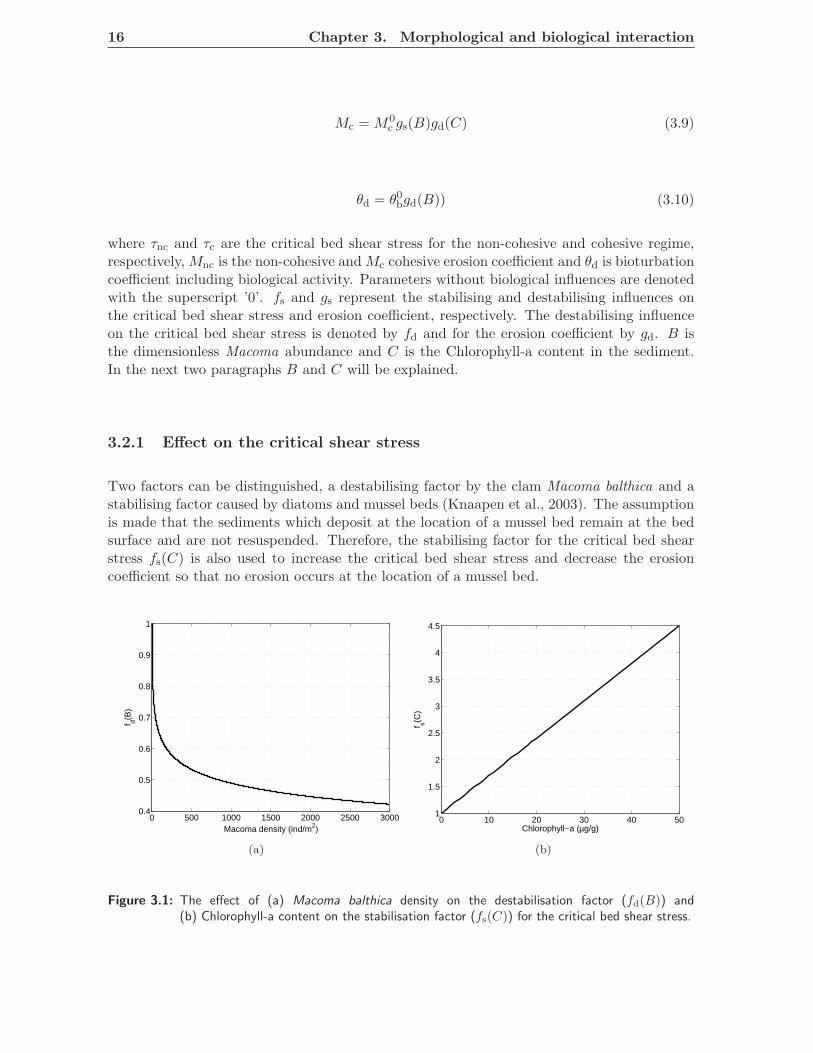
3.2.1 Effect on the critical shear stress
Two factors can be distinguished, a destabilising factor by the clam Macoma balthica and astabilising factor caused by diatoms and mussel beds (Knaapen et al., 2003). The assumptionis made that the sediments which deposit at the location of a mussel bed remain at the bedsurface and are not resuspended. Therefore, the stabilising factor for the critical bed shearstress fs(C) is also used to increase the critical bed shear stress and decrease the erosioncoefficient so that no erosion occurs at the location of a mussel bed.
0 500 1000 1500 2000 2500 30000.4
0.5
0.6
0.7
0.8
0.9
1
Macoma density (ind/m2)
f d(B)
(a)
0 10 20 30 40 501
1.5
2
2.5
3
3.5
4
4.5
Chlorophyll−a (µg/g)
f s(C)
(b)
Figure 3.1: The effect of (a) Macoma balthica density on the destabilisation factor (fd(B)) and(b) Chlorophyll-a content on the stabilisation factor (fs(C)) for the critical bed shear stress.

3.2 Parameterisation of biological activity 17
The expressions for the destabilising and stabilising factors are:
fd(B) = 0.0016 ln[Macoma∗]2 − 0.085 ln[Macoma∗] + 1 (3.11)
B =Macoma
Macomaref
fs(C) = 0.07[C] + 1 (3.12)
C =Chla
Chlaref
where B and C are made dimensionless using a reference density of 1 m−2 and a referencecontent of 1 µg/g. In Figure 3.1(a) the relationship between Macoma balthica density and thedestabilisation factor fd(B) is given. In Figure 3.1(b) the relation between the stabilisationfactor fs(C) and the Chlorophyll-a content is given.
3.2.2 Effect on the erosion coefficient
The destabilising effect on the erosion coefficient (M) is expressed by the following equation(Paarlberg et al., 2005):
gd(B) =b2γ
(b2 + γ[b1]B) I(3.13)
and the stabilising effect on the erosion coefficient by:
gs(C) = −0.018C + 1 (3.14)
where b1 = 0.995 and b2 = 5.08× 10⁻⁸, I the erosion coefficient without biological activity is4.68 × 10−8 m s−1 and γ the maximum erosion coefficient is 6 × 10⁻⁷. In Figure 3.2(a) therelation between the destabilisation factor (gd(B)) and the M. balthica density is given. The
0 500 1000 1500 2000 2500 30000
2
4
6
8
10
12
14
Macoma density (ind/m2)
g d(B)
(a)
0 10 20 30 40 500.1
0.2
0.3
0.4
0.5
0.6
0.7
0.8
0.9
1
Chlorophyll a (µg/g)
g s(C)
(b)
Figure 3.2: The effect of (a) Macoma balthica density on the destabilisation factor (gd(B)) and(b) Chlorophyll-a content on the stabilisation factor (gs(C)) for the erosion coefficient.

18 Chapter 3. Morphological and biological interaction
S-shaped curve (logistic function) starts at one because the factor gd is always larger thanone. If the factor is smaller than one, it will have an unwanted stabilising effect on the erosionrate.
3.3 Sand-mud-bio model
In the previous sections the parameterisation of biology and morphology is described. Todetermine the influence of biological activity on the suspended sediment transport in theFriesche zeegat, Eqs. 3.6 - 3.10 are implemented in the sand-mud model by Van Ledden(2003). In Figure 1.3 the setup of the original process-based sand-mud model is given. Thismodel is extended with the description of the biological activity and a schematisation is givenin Figure 3.3.
Sand & mud
transport
Flow
Bed level
Bed
composition
τcr
M
Bτ
Be
Stabilising
organisms
Destabilising
organisms
Figure 3.3: Set-up of the original sand-mud model included with influence of the biological activity (Paarl-berg et al., 2005).

Chapter 4
Model set-up of the reference
situation
In order to study the effects of the biological influence by stabilisers and destabilisers on thefine-grained sediment transport, first a model set-up of the reference situation is made. Thismodel set-up is based on the original process-based sand-mud model by Van Ledden (2003)with addition of the biologically parameters described in the previous chapter.
First, a description of the model simulation is given in. Second, a schematisation of the modelarea is given in. Finally, the boundary conditions and the initial conditions are described.
4.1 Simulation of the model
The process-based sand-mud model simulates two tides starting at high water. The durationof one tidal period is 12 hours and 24 minutes and the model uses a time-step of one minute.In order to decrease the model simulation time a morphological scaling factor is used. Asit name reveals, this scaling factor exaggerates the morphological features like the bed levelchange and bed level composition. The scaling factor is set at 116, this means that one singlesimulation of two tides is in fact 116 times two tides which approximately corresponds to 120days. In order to perform simulations longer than one third of a year, the morphological dataand the mud content of each simulation is saved and used as input for the next simulation. So,3 or 6 repeated simulations approximately correspond to one year or two years respectively.
During each simulation the first tidal period is used for spinning up the model, becausesmall artificial errors in the bed shear stress might easily spoil the initial bed level andcomposition (De Boer, 2002). The morphological computation starts at the beginning of thesecond tidal period. During the repeated simulations the first tidal period is also used forspinning up and only the results of the second tide are used to assess changes in bed leveland composition.

20 Chapter 4. Model set-up of the reference situation
20 40 60 80 1000
10
20
30
40
50
60
70
80
X (gridcell)
Y (
grid
cell)
westernboundary
easternboundary
northernboundary
North Sea
Ameland Schiermonnikoog
Engels−manplaat
Pinkegat
Zoutkamperlaag
−25
−20
−15
−10
−5
0
5
Figure 4.1: Numerical grid (X,Y) and depth contours (m) of the Friesche Zeegat. The open boundariesare situated in the North Sea, the basin is surrounded by closed boundaries in the east, southand west.
4.2 Computational grid and bathymetry
The numerical grid for the Friesche Zeegat is based on the topography of 1991. This resultedin a horizontal grid of 105 × 81 with a resolution of 250 to 600 m. In the center of the gridthe size of the cells is smaller than at the boundaries. The model area is approximately 20km wide (north south) and 35 km long (east west). The three open boundaries are located inthe east, west and north of the North Sea. The water sheds, areas where the tidal currentsmeet, south of Ameland and Schiermonnikoog are natural boundaries and almost show nointeraction with the adjacent tidal basins. Therefore these boundaries are assumed to beclosed. The dike situated in the south of the basin is also modelled as a closed boundary.The model area is shown in Figure 4.1.
4.3 Boundary conditions
4.3.1 Hydrodynamics
The boundary condition at the North Sea can be composed of the semi-diurnal (M2) andthe quarter-diurnal tide (M4), in addition to the mean water level (M0). The M2-tide is aprincipal lunar tidal component with a period of 12 hours and 24 minutes. The quarter-diurnal M4-tide is a non-linear overtide generated by the M2 signal in the region. The effectof a spring-neap cycle was not considered. Detailed information about the possible effect ofa spring-neap cycle on the long-term morphological behaviour and the tidal constituents is

4.3 Boundary conditions 21
Wierumergronden Huibertgat Western boundary Eastern boundary
M0 0.006 -0.036 0.019 -0.028M2 0.951 1.029 0.928 1.014M4 0.097 0.087 0.099 0.089
Table 4.1: Water level amplitudes at Wierumergronden, Huibertgat, Western and Eastern model bound-ary (Van Ledden, 2003).
presented in Van Ledden (2003).
The water level amplitudes of the M0, M2 and M4 tidal constituents are based on two wa-ter level stations (Wierumergronden and Huibertgat) near the eastern and western modelboundary (see Table 4.1). The station Wierumergronden is located inside the model area,approximately (25,75), but the station Huibertgat is situated about 5 km outside the east-ern boundary in the North Sea. Towards the eastern and western boundary the amplitudesare interpolated and extrapolated linearly and are taken constant along these boundaries.Between the eastern and western boundary the tidal characteristics vary linearly along thenorthern boundary.
The water column in vertical direction is divided in five layers with a distribution from thewater surface to the bed of 50, 30, 10, 5 and 5% of the local water depth (Van Ledden, 2003).
4.3.2 Waves
The effects of short waves on the bed shear stress is taken into account, whereas wave-current interactions are neglected. The effect of waves is calculated with the SWAN package(Delft3D). Steady wave fields are calculated at 4 moments during the tide: high water, low
20 40 60 80 100
10
20
30
40
50
60
70
80
X (gridcell)
Y (
grid
cell)
North Sea
Ameland Schiermonnikoog
Engels−manplaat
Pinkegatinlet
Zoutkamperlaaginlet
0
0.2
0.4
0.6
0.8
1
1.2
1.4
1.6
1.8
2
(a)
20 40 60 80 100
10
20
30
40
50
60
70
80
X (gridcell)
Y (
grid
cell)
North Sea
Ameland Schiermonnikoog
Engels−manplaat
Pinkegatinlet
Zoutkamperlaaginlet
0
0.2
0.4
0.6
0.8
1
1.2
1.4
1.6
1.8
2
(b)
Figure 4.2: Wave heights (m) during (a) maximum ebb currents and (b) low water.

22 Chapter 4. Model set-up of the reference situation
20 40 60 80 100
10
20
30
40
50
60
70
80
X (gridcell)
Y (
grid
cell)
North Sea
Ameland Schiermonnikoog
Engels−manplaat
Pinkegatinlet
Zoutkamperlaaginlet
0
0.2
0.4
0.6
0.8
1
1.2
1.4
1.6
1.8
2
(a)
20 40 60 80 100
10
20
30
40
50
60
70
80
X (gridcell)
Y (
grid
cell)
North Sea
Ameland Schiermonnikoog
Engels−manplaat
Pinkegatinlet
Zoutkamperlaaginlet
0
0.2
0.4
0.6
0.8
1
1.2
1.4
1.6
1.8
2
(b)
Figure 4.3: Wave heights (m) during (a) maximum flood currents and (b) high water.
water and at maximum ebb and flood current. In Figure 4.2 and 4.3 the four different wavefields are presented. A cyclic time frame is used to ensure that the waves are always calculatedat the same moment in time during the tidal period. The wave conditions are obtained frommeasurements buoys near the Friesche Zeegat and represent different values of the long termdistribution. The wave fields are linearly interpolated in time between the calculated wavetimes.
The long-term wind direction and the wave direction show a large spreading between SSWand NNE. The wave distribution has peaks between 240°N and 360°N (nautical notation),
Description Symbol Value Unit
Sand grain size d50 140 µmMud grain size d50 63 µmSediment density ρs 2650 kg/m3
Settling velocity sand ωs 0.015 m/sSettling velocity mud ωm 0.00025 m/sCritical erosion shear stress:
- Non-cohesive erosion τcr,s 0.25 N/m2
- Cohesive erosion τe 0.5 N/m2
Erosion coefficient:- Non-cohesive erosion Mnc 10−4 m/s- Cohesive erosion Me 10−8 m/s
Critical mud content pm,cr 0.3 -Coefficient for critical shear stress
for non-cohesive mixtures β 1.5 -Critical deposition shear stress mud τcr,d 0.15 N/m2
Table 4.2: Settings of the physical parameters of the reference computation.

4.4 Initial conditions 23
therefore a direction of 355°N is chosen (De Boer, 2002). This will result in waves approachingperpendicular to the coast of the backbarrier islands in the Wadden Sea. The wave drivencurrents along the coasts of the islands will almost be absent, which makes the neglecting ofthe wave-current interaction less significant.
4.4 Initial conditions
The applied sand concentration at the inflow of the open sea boundaries is kept constant forsuspended sand transport. The mud concentration offshore appears to be low (5 - 10 mg/l),but increases up to 100 mg/l at 5 - 10 km from the coast. Because the northern modelboundary is located approximately 10 km of the coast, a uniform mud concentration profileis used with a constant value of cm,0 = 100 mg/l at all open boundaries (Van Ledden, 2003).
In the reference situation the initial current velocity, water level and suspended sedimentconcentrations are set to zero. Also, the initial mud content is zero and the simulation startswith a full sand bed. The mud content at the end of each simulation is used as the initialmud content for the next simulation.

Chapter 5
Reference situation
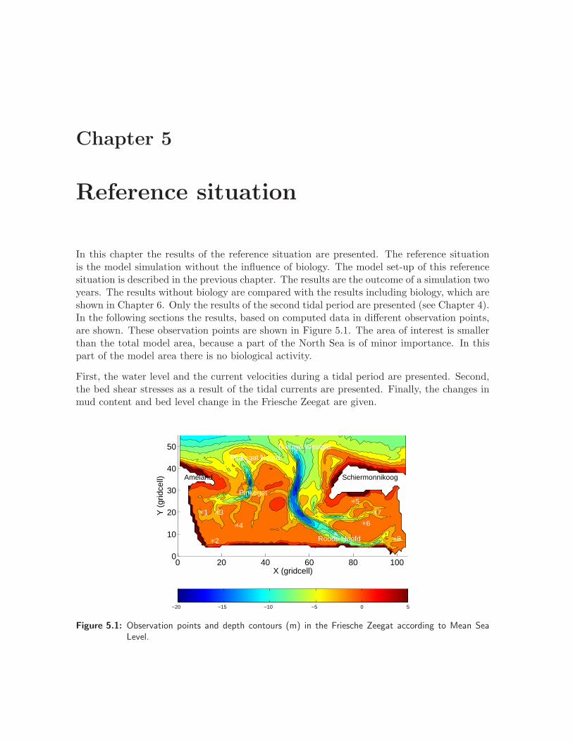
In this chapter the results of the reference situation are presented. The reference situationis the model simulation without the influence of biology. The model set-up of this referencesituation is described in the previous chapter. The results are the outcome of a simulation twoyears. The results without biology are compared with the results including biology, which areshown in Chapter 6. Only the results of the second tidal period are presented (see Chapter 4).In the following sections the results, based on computed data in different observation points,are shown. These observation points are shown in Figure 5.1. The area of interest is smallerthan the total model area, because a part of the North Sea is of minor importance. In thispart of the model area there is no biological activity.
First, the water level and the current velocities during a tidal period are presented. Second,the bed shear stresses as a result of the tidal currents are presented. Finally, the changes inmud content and bed level change in the Friesche Zeegat are given.
0 20 40 60 80 1000
10
20
30
40
50
X (gridcell)
Y (
grid
cell) Ameland Schiermonnikoog
1
2
3
4
Pinkegat
Pinkegat Noord
Nieuwe Westgat
Roode Hoofd
5
6
7
8
−20 −15 −10 −5 0 5
Figure 5.1: Observation points and depth contours (m) in the Friesche Zeegat according to Mean SeaLevel.

26 Chapter 5. Reference situation
5.1 Water level and tidal currents
The water level as a result of the the semi-diurnal (M2) and the quarter-diurnal tide (M4) (seeSection 4.3.1) is presented for the different observation points in the Friesche Zeegat. Thedepths of the observation points in the Pinkegat channel and the Zoutkamperlaag channelare shown in Table 5.1. The locations of these observation points are shown in Figure 5.1 andthe corresponding water levels during a simulation are presented in Figure 5.2(a) and 5.2(b).Location 2, 4, 5 and 6 are shallow which causes drying of these mud flats during ebb. Theminimum water level at location 2, 4, 5 and 6 does not correspond with the depth in Table 5.1.This is caused by the drying and flooding routine in Delft3D. The sand-mud model alwaysleaves a thin layer of water on the mud flats when the water level becomes lower than thebed level.
The amplitude of the tide in the deeper areas (Pinkegat and Nieuwe Westgat) is smaller thanthe amplitude in the shallow areas. Due to a decrease in water depth the tidal wave speedand wave length decrease, therefore the energy per unit area of the wave has to increase.This ’shoaling’-effect results in an increase of the tidal wave height, but the tidal wave periodremains the same. Especially, in Figure 5.2(b) these differences are clear, while in Figure 5.2(a)these differences are less significant. The propagation of the tidal wave through the basinresults in a difference in tidal phase at each observation point. The larger the distance betweenthe observation points the larger the tidal phase difference. This difference is especially visiblebetween observation point Nieuwe Westgat, Roode Hoofd and location 7 and 8.
An indication of the tidal induced current velocities for the 12 observation points is given inFigure 5.3. The presented velocities are taken from the fifth layer of the water column, whichis the closest to the bed surface at a height of 5% of the local water depth. This height ischosen because the highest current velocity is expected to be found close to the bed surface,which will generate the highest bed shear stress. During ebb and flood the largest tidal
12 18 24−1.4
−1.2
−1
−0.8
−0.6
−0.4
−0.2
0
0.2
0.4
0.6
0.8
1
1.2
1.4
Time (h)
Wat
er le
vel (
m)
low water high water
PinkegatPinkegat NoordLocation 1Location 2Location 3Location 4
(a)
12 18 24−1.4
−1.2
−1
−0.8
−0.6
−0.4
−0.2
0
0.2
0.4
0.6
0.8
1
1.2
1.4
Time (h)
Wat
er le
vel (
m)
low water high water
Nieuwe WestgatRoode HoofdLocation 5Location 6Location 7Location 8
(b)
Figure 5.2: Water level during a single tidal period at location: (a) 1 - 4, Pinkegat and Pinkegat Noordand (b) 5 - 8, Nieuwe Westgat and Roode Hoofd.

5.2 Bed shear stress 27
12 18 240
0.1
0.2
0.3
0.4
0.5
0.6
0.7
Time (h)
Cur
rent
vel
ocity
(m
/s)
low water high water
PinkegatPinkegat NoordLocation 1Location 2Location 3Location 4
(a)
12 18 240
0.1
0.2
0.3
0.4
0.5
0.6
0.7
Time (h)
Cur
rent
vel
ocity
(m
/s)
low water high water
Nieuwe WestgatRoode HoofdLocation 5Location 6Location 7Location 8
(b)
Figure 5.3: Current velocities (m/s) during a tidal period at location: (a) 1 - 4, Pinkegat and PinkegatNoord and (b) 5 - 8, Nieuwe Westgat and Roode Hoofd.
currents can be seen and during low and high water the tidal currents are at its minimum.
The largest maximum ebb and flood current velocities can be found in both channels, locationPinkegat and Pinkegat Noord (see Figure 5.3(a)) and location Nieuwe Westgat and RoodeHoofd (see Figure 5.3(b)). Because of the earlier explained ’shoaling’-effect, a decrease inwater depth results in a decrease in current velocity. The decrease in current velocities at theshallow mud flats is clearly visible, however the difference between ebb and flood velocities foreach location is not very significant. Location Pinkegat, Pinkegat Noord, Roode Hoofd, 1 and4 show higher maximum flood currents than maximum ebb currents. At the other locationsthe maximum ebb current is more or less equal or slightly stronger than the maximum floodcurrent.
Figure 5.4 shows the maximum ebb and flood currents, but also the difference between thesetwo. In Figure 5.4(c) the negative values for the current velocity are ebb dominated andthe positive values are flood dominated. Looking at these figures, the differences betweenmaximum ebb and flood currents are more clearly visible. Because of the tidal wave propa-gation through the basin not all maximum ebb and flood currents occur at the same time forthe entire area. The minimum and maximum currents shown, are taken when the maximumebb and flood currents occur at location Roode Hoofd. Figure 5.4(c) shows an overall largerflood current than ebb current, not only in the channels but also on the mud flats. Takinginto account that Figure 5.4 shows the moments of approximately the maximum ebb andflood velocities in the entire basin, the differences in some areas can be slightly exaggeratedor underestimated. Because of the constant mud concentration of 100 mg/l (see 4.3) at theboundaries in the North Sea during each simulation, an increase of the mud content in theentire basin is expected.

28 Chapter 5. Reference situation
0 20 40 60 80 1000
10
20
30
40
50
X (gridcell)
Y (
grid
cell)
0 0.1 0.2 0.3 0.4 0.5 0.6 0.7 0.8 0.9 1
(a)
0 20 40 60 80 1000
10
20
30
40
50
X (gridcell)
Y (
grid
cell)
0 0.1 0.2 0.3 0.4 0.5 0.6 0.7 0.8 0.9 1
(b)
0 20 40 60 80 1000
10
20
30
40
50
X (gridcell)
Y (
grid
cell)
−0.5 −0.4 −0.3 −0.2 −0.1 0 0.1 0.2 0.3 0.4 0.5
(c)
Figure 5.4: Tidal current velocities (m/s) in the Friesche Zeegat: (a) maximum ebb, (b) maximum floodcurrents and (c) difference between the maximum ebb and flood currents (positive valueindicates higher flood current velocities, negative value indicates higher ebb current velocity).
5.2 Bed shear stress
In Figure 5.5 the bed shear stress is presented for all observation points. In both figures thecritical bed shear stress in the non-cohesive regime and the critical bed shear stress for thecohesive regime are shown, where the critical bed shear stress for non-cohesive mixtures is0.25 N/m2 and 0.5 N/m2 for cohesive mixtures. The switch from a non-cohesive to a cohesiveregime takes place if the mud content exceeds 30% (pm,cr).
From Figure 5.5, one can see that the maximum bed shear stress at location 1, 2 and 5 doesnot exceed the critical bed shear stress for non cohesive mixtures (τnc). At location 4 and6 the bed shear stress does not exceed the critical bed shear stress in the cohesive regime(τc). When the bed shear stress is smaller than the critical bed shear stress, no erosion willoccur. At all other locations, with a depth larger than 2 m, the bed shear stress exceeds thecritical bed shear stress. This means that in these areas erosion occurs. The percentage intime exceeding the critical bed shear stress in the cohesive and non-cohesive regime during

5.2 Bed shear stress 29
12 18 240
0.1
0.2
0.3
0.4
0.5
0.6
0.7
0.8
0.9
1
1.1
1.2
1.3
Time (h)
τ (N
/m2 )
low water high water
PinkegatPinkegat NoordLocation 1Location 2Location 3Location 4τ
cr,cτ
cr,nc
(a)
12 18 240
0.1
0.2
0.3
0.4
0.5
0.6
0.7
0.8
0.9
1
1.1
1.2
1.3
Time (h)
τ (N
/m2 )
low water high water
WestgatHoofdLocation 5Location 6Location 7Location 8τ
cr,cτ
cr,nc
(b)
Figure 5.5: Bed shear stress (N/m2) during a tidal period at location: (a) 1 - 4 and Pinkegat (Noord)and (b) 5 - 8, Nieuwe Westgat and Roode Hoofd. The horizontal lines represent the criticalbed shear stress for non-cohesive mixtures (τcr,nc) and for cohesive mixtures (τcr,c).
one tidal period for all observation points is shown in Table 5.1.
The comparison of Figure 5.3 with Figure 5.5 indicates that small current velocities resultin low bed shear stresses and in these areas no erosion occurs. In the deeper areas, wherehigh current velocities and high bed shear stresses occur, erosion of the bed leads to bedload transport or suspended sediment transport. The latter is important for this research,because the fine-grained sediment transport is believed to be influenced by biological activity.As described before in Chapter 3.1.2, suspended sediment transport is also influenced byupstream conditions. The passing water is influenced by local flow conditions upstream of
Depth (m) % exceedingLocation τnc τc
1 1.25 0 02 0.12 0 03 2.39 45 384 0.42 35 05 0.19 0 06 0.13 5 07 2.21 58 268 2.25 74 46Pinkegat 15.76 60 42Pinkegat Noord 3.80 79 53Nieuwe Westgat 9.31 77 62Roode Hoofd 9.18 80 66
Table 5.1: Percentage in time exceeding τnc and τc during one tidal period for each observation point.

30 Chapter 5. Reference situation
the area of interest.
During 60 - 80% of the tidal period the critical bed shear stress in the non-cohesive regimeis exceeded for location 7, 8, Pinkegat, Nieuwe Westgat en Roode Hoofd. This means thaterosion occurs and this results in bed load and suspended sediment transport. At the shallowmud flats (location 1, 2, 4, 5 and 6) bed shear stresses are very small and if current velocitiesare small enough, no erosion occurs.
The switch between the non-cohesive and cohesive regime lies around a critical mud contentof 30%. The critical bed shear stress is doubled and for locations 7, 8, Pinkegat, NieuweWestgat and Roode Hoofd about 50% of the time, no erosion will take place, this is causedby the cohesive bed which forms a coherent mass caused by the electrochemical interactionsbetween the sediment particles. This does not mean, that no suspended sediment transportwill occur, once in suspension, particles can remain in suspension when current velocities arehigh enough.
5.3 Suspended sediment
The computed suspended mud concentration is measured in the lower 5% of the water column,at the same height above the bed surface as the current velocities (see Section 5.1). Thesuspended mud concentration during the tidal period is shown in Figure 5.6. It can be notedthat for location 1, 5, 6 and 7 the suspended mud concentration are excessively high duringlow water. In the model a thin layer of water remains on the mud flats during low water,because of drying this results in very high unrealistic mud concentrations. Location 2, 4, 5and 6 are shallow and during low water these mud flats emerge, but only at location 5 and 6this results in high suspended mud concentrations.
12 18 240
1
2
3
4
5
6
7
8
9
10
11
12
Time (h)
C (
g/l)
low water high water
PinkegatPinkegat NoordLocation 1Location 2Location 3Location 4
(a)
12 18 240
1
2
3
4
5
6
7
8
9
10
11
12
Time (h)
C (
g/l)
low water high water
Nieuwe WestgatRoode HoofdLocation 5Location 6Location 7Location 8
(b)
Figure 5.6: Suspended mud concentration (g/l) profiles during a tidal period in: (a) location 1 - 4 andPinkegat and (b) location 5 - 8, Nieuwe Westgat and Roode Hoofd.

5.3 Suspended sediment 31
Pinkegat Noord Nieuwe WestgatEbb Flood Ebb Flood
Concentration (g/l) 0.41 0.45 0.23 0.27
Table 5.2: Average suspended mud concentration (g/l) during the ebb and flood period.
Looking at the computed suspended mud concentrations during ebb and flood in the Zoutkam-perlaag channel and the Pinkegat channel, the following differences can be noted. In Table 5.2the average suspended mud concentration for location Nieuwe Westgat and Pinkegat Noordduring ebb and flood is shown. At location Nieuwe Westgat the average concentration duringebb is 0.23 g/l and during flood is 0.27 g/l. At location Pinkegat Noord the suspended mudconcentrations are 0.41 g/l during ebb and 0.45 g/l during flood. These two locations are cho-sen because these are positioned in a tidal channel, where the tidal flow during ebb and floodis more or less in the same direction. Assuming that the amount of water flowing through theZoutkamperlaag is twice the amount of water flowing through the Pinkegat channel duringebb and flood Van Leeuwen et al. (2003), the amount of mud remaining in the tidal basinduring one tidal period is estimated at 9,500 ton.
To give an indication of the reliability of the results, the locations Nieuwe Westgat and RoodeHoofd are compared with observed data obtained at the Zoutkamperlaag (corresponds withlocation Nieuwe Westgat) and Roode Hoofd from 1973 - 2003 shown in Figure 5.7. An outlineof all concentrations is given in Table 5.3.
The observed average concentration for the Zoutkamperlaag is 0.082 g/l and the Roode Hoofdand 0.069 g/l (directly from the website: http://www.waterbase.nl). These are low comparedto the computed concentration shown in Figure 5.6, 0.26 g/l for location Nieuwe Westgatand 0.52 g/l for location Roode Hoofd. The results show the concentration during a singletidal period instead of a long-term calculation, like the period during which the observed dataare obtained. It is more likely to compare the computed maximum concentrations with themaximum observed concentrations.
The maximum observed mud concentration in the Zoutkamperlaag is 0.38 g/l and the accom-panying computed concentration in the Nieuwe Westgat is 0.59 g/l. The maximum observedconcentration at Roode Hoofd is 0.34 g/l and the corresponding computed concentration is0.66 g/l. The maximum observed and computed mud concentration are in the same order(10−1), while the average observed mud concentrations are about a factor 10 lower (10−2)than the computed average mud concentrations. The computed values for the maximum sus-
Average mud concentration (g/l) Maximum mud concentration (g/l)Observed Computed Observed Computed
Nieuwe Westgat 0.082 0.24 0.38 0.59Roode Hoofd 0.069 0.49 0.34 0.66
Table 5.3: Observed and computed average and maximum suspended mud concentrations for locationNieuwe Westgat and Roode Hoofd.

32 Chapter 5. Reference situation
19731976 1979 1982 1985 1988 1991 1994 1997 2000 20030
0.05
0.1
0.15
0.2
0.25
0.3
0.35
0.4
Time (year)
Sus
pend
ed s
edim
ent (
g/l)
(a)
1973 1976 1979 1982 1985 1988 1991 1994 1997 2000 20030
0.05
0.1
0.15
0.2
0.25
0.3
0.35
0.4
Time (year)
Sus
pend
ed s
edim
ent (
g/l)
(b)
Figure 5.7: Observed suspended sediment concentration (g/l) at (a) Nieuwe Westgat and (b) Roode Hoofdfrom 1973 - 2003 (http://www.waterbase.nl). The horizontal lines represent the averageconcentration during that period.
pended sediment concentration are almost twice as high as the observed data. As one can seefrom Table 5.3, the observed concentrations are larger at location Nieuwe Westgat than atlocation Roode Hoofd, while this is the opposite for the computed mud concentrations. It isuncertain at which moment during the tidal period the observed data is taken and the heightat which the measurements are taken is not available.
Figure 5.8: Observed mud content in the Friesche Zeegat (Van Rijsewijk, 2002).

5.4 Mud content 33
0 20 40 60 80 1000
10
20
30
40
50
X (gridcell)
Y (
grid
cell) Ameland Schiermonnikoog
Engels−manplaat
0 10 20 30 40 50 60 70 80 90 100
(a)
0 20 40 60 80 1000
10
20
30
40
50
X (gridcell)
Y (
grid
cell) Ameland Schiermonnikoog
Engels−manplaat
0 10 20 30 40 50 60 70 80 90 100
(b)
Figure 5.9: Mud content (%) after (a) 1 year and (b) 2 years.
5.4 Mud content
In Figure 5.9 the development of the computed mud content in the top layer of the bed surfaceis presented. The model starts with a plain sand bed and as can be seen, after 1 year there isa significant increase in mud content. High concentrations of mud (about 40%) can be foundclose to the shore and on the mud flats. Exceeding the critical mud content of 30% results ina switch from a non-cohesive to a cohesive regime. The increased critical bed shear stress anddecreased erosion coefficient will lead to less erosion and most likely more mud deposition.
After two years, in a large area of the basin, the critical mud content of 30% is exceeded. Inthe eastern part of the tidal basin and also along the western water shed, high mud contentcan be observed. Looking at the center of the basin, the mud content remains about 20%.After 4 and 8 years, the rapid increase in mud content becomes smaller and the system tendsto an equilibrium. Comparing Figure 5.4 with Figure 5.9 and 5.10 one can see that when the
0 20 40 60 80 1000
10
20
30
40
50
X (gridcell)
Y (
grid
cell) Ameland Schiermonnikoog
Engels−manplaat
0 10 20 30 40 50 60 70 80 90 100
(a)
0 20 40 60 80 1000
10
20
30
40
50
X (gridcell)
Y (
grid
cell) Ameland Schiermonnikoog
Engels−manplaat
0 10 20 30 40 50 60 70 80 90 100
(b)
Figure 5.10: Mud content (%) after (a) 4 year and (b) 8 years.
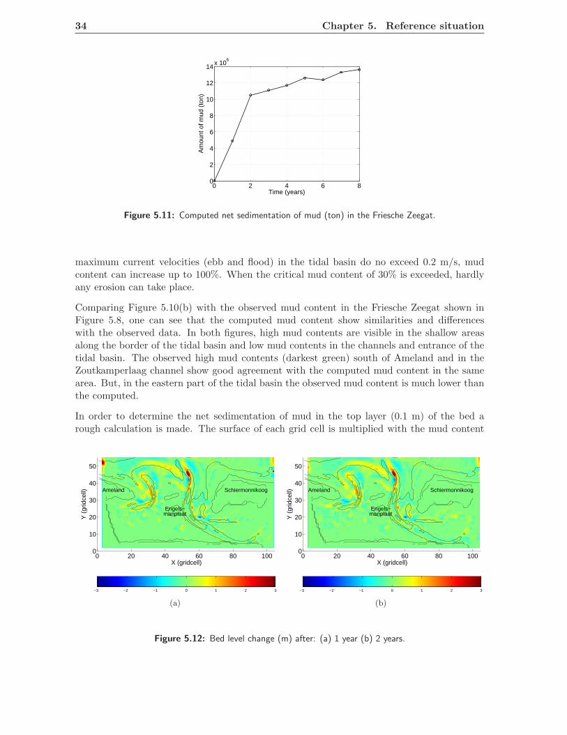
34 Chapter 5. Reference situation
0 2 4 6 80
2
4
6
8
10
12
14x 10
6
Time (years)A
mou
nt o
f mud
(to
n)
Figure 5.11: Computed net sedimentation of mud (ton) in the Friesche Zeegat.
maximum current velocities (ebb and flood) in the tidal basin do no exceed 0.2 m/s, mudcontent can increase up to 100%. When the critical mud content of 30% is exceeded, hardlyany erosion can take place.
Comparing Figure 5.10(b) with the observed mud content in the Friesche Zeegat shown inFigure 5.8, one can see that the computed mud content show similarities and differenceswith the observed data. In both figures, high mud contents are visible in the shallow areasalong the border of the tidal basin and low mud contents in the channels and entrance of thetidal basin. The observed high mud contents (darkest green) south of Ameland and in theZoutkamperlaag channel show good agreement with the computed mud content in the samearea. But, in the eastern part of the tidal basin the observed mud content is much lower thanthe computed.
In order to determine the net sedimentation of mud in the top layer (0.1 m) of the bed arough calculation is made. The surface of each grid cell is multiplied with the mud content
0 20 40 60 80 1000
10
20
30
40
50
X (gridcell)
Y (
grid
cell) Ameland Schiermonnikoog
Engels−manplaat
−3 −2 −1 0 1 2 3
(a)
0 20 40 60 80 1000
10
20
30
40
50
X (gridcell)
Y (
grid
cell) Ameland Schiermonnikoog
Engels−manplaat
−3 −2 −1 0 1 2 3
(b)
Figure 5.12: Bed level change (m) after: (a) 1 year (b) 2 years.
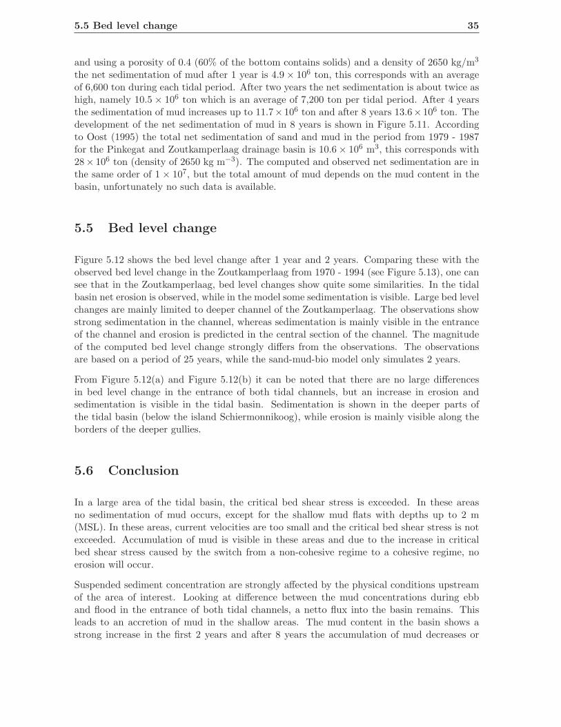
5.5 Bed level change 35
and using a porosity of 0.4 (60% of the bottom contains solids) and a density of 2650 kg/m3
the net sedimentation of mud after 1 year is 4.9 × 10⁶ ton, this corresponds with an averageof 6,600 ton during each tidal period. After two years the net sedimentation is about twice ashigh, namely 10.5 × 10⁶ ton which is an average of 7,200 ton per tidal period. After 4 yearsthe sedimentation of mud increases up to 11.7×10⁶ ton and after 8 years 13.6×10⁶ ton. Thedevelopment of the net sedimentation of mud in 8 years is shown in Figure 5.11. Accordingto Oost (1995) the total net sedimentation of sand and mud in the period from 1979 - 1987for the Pinkegat and Zoutkamperlaag drainage basin is 10.6 × 10⁶ m3, this corresponds with28× 106 ton (density of 2650 kg m−3). The computed and observed net sedimentation are inthe same order of 1 × 10⁷, but the total amount of mud depends on the mud content in thebasin, unfortunately no such data is available.
5.5 Bed level change
Figure 5.12 shows the bed level change after 1 year and 2 years. Comparing these with theobserved bed level change in the Zoutkamperlaag from 1970 - 1994 (see Figure 5.13), one cansee that in the Zoutkamperlaag, bed level changes show quite some similarities. In the tidalbasin net erosion is observed, while in the model some sedimentation is visible. Large bed levelchanges are mainly limited to deeper channel of the Zoutkamperlaag. The observations showstrong sedimentation in the channel, whereas sedimentation is mainly visible in the entranceof the channel and erosion is predicted in the central section of the channel. The magnitudeof the computed bed level change strongly differs from the observations. The observationsare based on a period of 25 years, while the sand-mud-bio model only simulates 2 years.
From Figure 5.12(a) and Figure 5.12(b) it can be noted that there are no large differencesin bed level change in the entrance of both tidal channels, but an increase in erosion andsedimentation is visible in the tidal basin. Sedimentation is shown in the deeper parts ofthe tidal basin (below the island Schiermonnikoog), while erosion is mainly visible along theborders of the deeper gullies.
5.6 Conclusion
In a large area of the tidal basin, the critical bed shear stress is exceeded. In these areasno sedimentation of mud occurs, except for the shallow mud flats with depths up to 2 m(MSL). In these areas, current velocities are too small and the critical bed shear stress is notexceeded. Accumulation of mud is visible in these areas and due to the increase in criticalbed shear stress caused by the switch from a non-cohesive regime to a cohesive regime, noerosion will occur.
Suspended sediment concentration are strongly affected by the physical conditions upstreamof the area of interest. Looking at difference between the mud concentrations during ebband flood in the entrance of both tidal channels, a netto flux into the basin remains. Thisleads to an accretion of mud in the shallow areas. The mud content in the basin shows astrong increase in the first 2 years and after 8 years the accumulation of mud decreases or
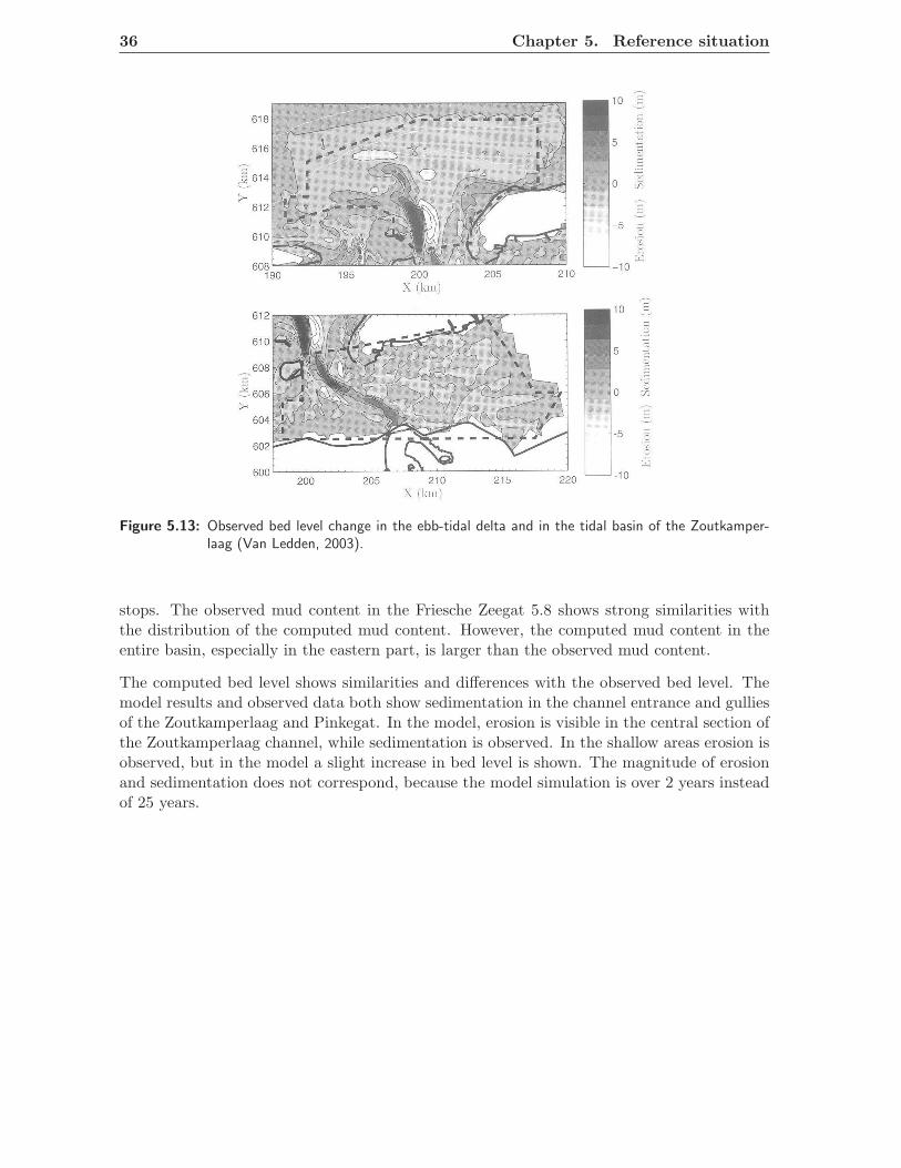
36 Chapter 5. Reference situation
Figure 5.13: Observed bed level change in the ebb-tidal delta and in the tidal basin of the Zoutkamper-laag (Van Ledden, 2003).
stops. The observed mud content in the Friesche Zeegat 5.8 shows strong similarities withthe distribution of the computed mud content. However, the computed mud content in theentire basin, especially in the eastern part, is larger than the observed mud content.
The computed bed level shows similarities and differences with the observed bed level. Themodel results and observed data both show sedimentation in the channel entrance and gulliesof the Zoutkamperlaag and Pinkegat. In the model, erosion is visible in the central section ofthe Zoutkamperlaag channel, while sedimentation is observed. In the shallow areas erosion isobserved, but in the model a slight increase in bed level is shown. The magnitude of erosionand sedimentation does not correspond, because the model simulation is over 2 years insteadof 25 years.

Chapter 6
Influence biological activity
In this chapter the result of the simulations with biological activity are presented. All figuresshow the results after 2 years of simulation1, which are compared with the results presentedin the previous chapter. To examine the influence of biological activity on the fine-grainedsediment transport four scenarios are simulated. A scenario with a destabilising effect causedby the bivalve Macoma balthica, a stabilising effect caused by algae, a stabilising effect causedby mussel beds and a scenario with a combination of all organisms.
In the first two sections the influence of the biological activity on the bed shear stress anderosion coefficient is described. Subsequently, the mud content for each scenario and thedifference with the reference situation are shown. Next, the changes in bed level for eachscenario compared to the reference situation is presented and finally, a summary of the resultsis given.
6.1 Bed shear stress
Biological activity affects the critical bed shear stress. In Table 6.1 the observation points withtheir corresponding correction factor for the critical bed shear stress and the corrected criticalbed shear stress in the non-cohesive and cohesive regime are presented for each scenario. Thecritical bed shear stress in the non-cohesive regime is 0.25 N/m2 and in the cohesive regime0.50 N/m2. The locations Pinkegat, Pinkegat Noord, Nieuwe Westgat en Roode Hoofd arenot presented. At these locations there is no biological activity and therefore the criticalbed shear stress is not corrected. The exceeding of the critical bed shear stress remains thesame as given in Table 5.1. This also applies to location 1, 3, 7 and 8. Because there is noinfluence of diatoms and mussel beds at these locations, the critical bed shear stress for thesetwo scenarios is not affected. On the other hand, it is affected by Macoma balthica.
Comparing Table 5.1 with Table 6.2, one can see that for the scenario with M. balthica thecritical bed shear stress (non-cohesive and cohesive) is lowered. In the non-cohesive regimeall locations exceed the critical bed shear stress and at these locations erosion will occur.
1The model with biological activity could not be simulated for a period of 8 years, because of errors duringthe simulation.

38 Chapter 6. Influence biological activity
M. balthica Diatoms Mussel beds Combination
Loc. Bτ τnc τc Bτ τnc τc Bτ τnc τc Bτ τnc τc
1 0.62 0.16 0.31 - - - - - - 0.62 0.16 0.312 0.48 0.12 0.24 3.42 0.81 1.62 4.50 1.13 2.25 2.16 0.54 1.083 0.62 0.16 0.31 - - - - - - 0.62 0.16 0.314 0.48 0.12 0.24 1.99 0.50 1.00 4.50 1.13 2.25 2.16 0.54 1.085 0.48 0.12 0.24 3.24 0.81 1.62 4.50 1.13 2.25 2.16 0.54 1.086 0.48 0.12 0.24 3.24 0.81 1.62 4.50 1.13 2.25 2.16 0.54 1.087 0.62 0.16 0.31 - - - - - - 0.62 0.16 0.318 0.62 0.16 0.31 - - - - - - 0.62 0.16 0.31
Table 6.1: Observation points with corresponding correction factor for the critical bed shear stress (Bτ =fd(B) · fs(C)) [-] and corrected critical bed shear stress [N/m2] for each scenario.
Looking at a depth range from MSL to 3 m water depth in the entire basin , it is likely that ifthe critical mud content is not exceeded erosion will occur, but this strongly depends on themagnitude of the local current velocities. In the cohesive regime the critical bed shear stressat location 1, 2, 5 and 6 is still to high to have an influence on erosion.
The scenarios with diatoms and mussel beds both affect the critical bed shear stress. In thecohesive and non-cohesive regime the critical bed shear stress is not exceeded for location 2,4, 5 and 6. In the entire basin from MSL to 1 m water depth, the diatoms increase the criticalbed shear stress, which results in no erosion. At the locations of the mussel beds, no diatomsare present. The critical bed shear stress is only affected by the mussel beds and at theselocations no erosion occurs.
In the scenario with the influence of all organisms, one can see that where M. Balthica ispresent a decrease in bed shear stress and an increase in erosion is expected. The combinationof M. Balthica and the mussel beds at location 2, 4, 5 and 6 results in an increase in criticalbed shear stress. Where no mussel beds are present it depends on the Chlorophyll- a content
Reference M. balthica Diatoms Mussel beds Combination
% exceeding % exceeding % exceeding % exceeding % exceedingLocation τnc τc τnc τc τnc τc τnc τc τnc τc
1 0 0 20 0 - - - - 20 02 0 0 7 0 0 0 0 0 0 03 45 38 71 58 - - - - 71 584 35 0 59 38 0 0 0 0 0 05 0 0 52 0 0 0 0 0 0 06 5 0 57 0 0 0 0 0 0 07 58 26 75 70 - - - - 75 708 74 46 75 70 - - - - 75 70
Table 6.2: Percentage in time exceeding the critical bed shear stress in the non-cohesive (τc) and cohesiveregime and (τc) for each observation point and scenario.

6.2 Erosion coefficient 39
if the critical bed shear stress increases or decreases. The M. Balthica density from MSL to1 m water depth is 1078 individuals per m2, the destabilising factor (fd(B)) is 0.62. In orderto have an increase on the critical bed shear stress, the stabilising factor (fs(C)) has to belarger than 1.61. Looking at Figure 3.2(b), this value is reached at a Chlorophyll- a contentof approximately 9 µg/g. From Table 2.2 it can be noted that this Chlorophyll- a content isexceeded below an average water depth of 0.5 m. It is likely that from mean sea level to awater depth of 0.5 m, the critical bed shear stress increases in the entire basin as a result ofthe stabilising effect of the diatoms.
6.2 Erosion coefficient
In Table 6.3 an outline of the correction factors for the erosion coefficient is given. Thedestabilising effect of M. Balthica has the largest contribution to the benthos correction factorfor the critical erosion coefficient. Even with a significant stabilising effect of the mussel beds,in combination with M. Balthica, the erosion coefficient still increases. Looking at the waterdepth from MSL to 3 m, the destabilising effect of M. Balthica results in an increase of theerosion coefficient in the entire basin.
Location M. balthica Diatoms Mussel beds Combination
1 1.78 - - 1.782 12.17 0.42 0.10 1.223 1.78 - - 1.784 12.17 0.75 0.10 1.225 12.17 0.42 0.10 1.226 12.17 0.42 0.10 1.227 1.78 - - 1.788 1.78 - - 1.78
Table 6.3: Observation points with corresponding correction factor for the erosion rate (Be =gd(B) · gs(C)) [-].
6.3 Mud content
In this section the difference between the mud content in the Friesche Zeegat with and withoutbiological activity is presented. Based on the influence of the biology on the critical bed shearstress and the erosion coefficient, it is expected that the simulation with Macoma balthicashows a decrease of the mud content, the diatoms and mussel beds increase the mud contentand a combination of all organisms results in a slower increase of the mud content than in thereference situation. The difference is determined by subtracting the reference situation fromthe simulation including biological activity.
In Figure 6.1(b) it is clearly visible that there is a destabilising effect caused by M. balthica. Inthe area with depths up to 3 meters the mud content is 10 - 30% smaller than in the reference

40 Chapter 6. Influence biological activity
0 20 40 60 80 1000
10
20
30
40
50
X (gridcell)
Y (
grid
cell) Ameland Schiermonnikoog
Engels−manplaat
0 10 20 30 40 50 60 70 80 90 100
(a)
0 20 40 60 80 1000
10
20
30
40
50
X (gridcell)
Y (
grid
cell) Ameland Schiermonnikoog
Engels−manplaat
−50 −40 −30 −20 −10 0 10 20 30 40 50
(b)
Figure 6.1: Destabilising effect caused by the M. balthica: (a) mud content (%) in the top layer of the bedand (b) difference in mud content (%). ’+’ denotes areas where the mud content increasesand ’-’ denotes a decrease of the mud content as a result from the influence of biology.
situation and in the more shallow areas up to 50%. This is due to the sudden increase ofM. balthica (from 129 - 1078 individuals per m2). In the areas where no M. balthica is present,e.g. the channels and gullies, no differences are visible. In some areas, around gridpoint(25,30), along the border of the eastern water shed and in the Zoutkamperlaag channel neargridpoint (60,15) and (85,5), the erosion and redistribution of mud results in a slight increasein mud content. The total amount of mud that remains in the basin after 2 years is estimatedat 4.9 × 10⁶ ton (for the calculation see Section 5.4). This is less than half of the amount
0 20 40 60 80 1000
10
20
30
40
50
X (gridcell)
Y (
grid
cell) Ameland Schiermonnikoog
Engels−manplaat
0 10 20 30 40 50 60 70 80 90 100
(a)
0 20 40 60 80 1000
10
20
30
40
50
X (gridcell)
Y (
grid
cell) Ameland Schiermonnikoog
Engels−manplaat
−50 −40 −30 −20 −10 0 10 20 30 40 50
(b)
Figure 6.2: Stabilising effect caused by algae: (a) mud content (%) in the top layer of the bed and (b)difference in mud content (%). ’+’ denotes areas where the mud content increases and ’-’denotes a decrease of the mud content as a result from the influence of biology.
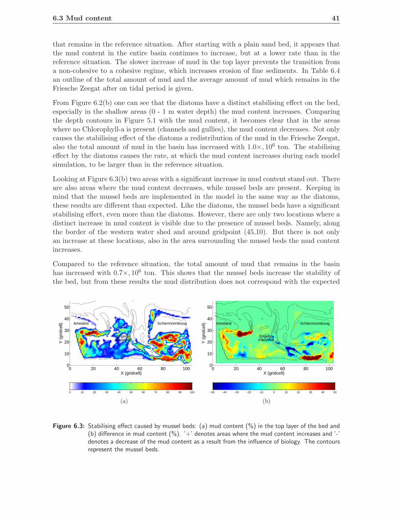
6.3 Mud content 41
that remains in the reference situation. After starting with a plain sand bed, it appears thatthe mud content in the entire basin continues to increase, but at a lower rate than in thereference situation. The slower increase of mud in the top layer prevents the transition froma non-cohesive to a cohesive regime, which increases erosion of fine sediments. In Table 6.4an outline of the total amount of mud and the average amount of mud which remains in theFriesche Zeegat after on tidal period is given.
From Figure 6.2(b) one can see that the diatoms have a distinct stabilising effect on the bed,especially in the shallow areas (0 - 1 m water depth) the mud content increases. Comparingthe depth contours in Figure 5.1 with the mud content, it becomes clear that in the areaswhere no Chlorophyll-a is present (channels and gullies), the mud content decreases. Not onlycauses the stabilising effect of the diatoms a redistribution of the mud in the Friesche Zeegat,also the total amount of mud in the basin has increased with 1.0×, 106 ton. The stabilisingeffect by the diatoms causes the rate, at which the mud content increases during each modelsimulation, to be larger than in the reference situation.
Looking at Figure 6.3(b) two areas with a significant increase in mud content stand out. Thereare also areas where the mud content decreases, while mussel beds are present. Keeping inmind that the mussel beds are implemented in the model in the same way as the diatoms,these results are different than expected. Like the diatoms, the mussel beds have a significantstabilising effect, even more than the diatoms. However, there are only two locations where adistinct increase in mud content is visible due to the presence of mussel beds. Namely, alongthe border of the western water shed and around gridpoint (45,10). But there is not onlyan increase at these locations, also in the area surrounding the mussel beds the mud contentincreases.
Compared to the reference situation, the total amount of mud that remains in the basinhas increased with 0.7×, 106 ton. This shows that the mussel beds increase the stability ofthe bed, but from these results the mud distribution does not correspond with the expected
0 20 40 60 80 1000
10
20
30
40
50
X (gridcell)
Y (
grid
cell) Ameland Schiermonnikoog
Engels−manplaat
0 10 20 30 40 50 60 70 80 90 100
(a)
0 20 40 60 80 1000
10
20
30
40
50
X (gridcell)
Y (
grid
cell) Ameland Schiermonnikoog
Engels−manplaat
−50 −40 −30 −20 −10 0 10 20 30 40 50
(b)
Figure 6.3: Stabilising effect caused by mussel beds: (a) mud content (%) in the top layer of the bed and(b) difference in mud content (%). ’+’ denotes areas where the mud content increases and ’-’denotes a decrease of the mud content as a result from the influence of biology. The contoursrepresent the mussel beds.

42 Chapter 6. Influence biological activity
0 20 40 60 80 1000
10
20
30
40
50
X (gridcell)
Y (
grid
cell) Ameland Schiermonnikoog
Engels−manplaat
0 10 20 30 40 50 60 70 80 90 100
(a)
0 20 40 60 80 1000
10
20
30
40
50
X (gridcell)
Y (
grid
cell) Ameland Schiermonnikoog
Engels−manplaat
−50 −40 −30 −20 −10 0 10 20 30 40 50
(b)
Figure 6.4: Combination of (de)stabilising effect caused by all organisms: (a) mud content (%) in the toplayer of the bed and (b) difference in mud content (%). ’+’ denotes areas where the mudcontent increases and ’-’ denotes a decrease of the mud content as a result from the influenceof biology.
distribution. The decrease of mud content in certain areas is probably due to the redistributionof mud to the areas with high concentrations of mud. The increase of mud content aroundgridpoint (30,30) and (85,5) is probably caused by an error in the model. Unfortunately, theerror could not be identified.
In Figure 6.4(b) all three scenarios are combined to show the effect of destabilisers andstabilisers on the mud distribution. It is clearly visible that the influence of the destabilisingM. balthica is dominant. Except for two spots where an increase in mud content can be seen(Pinkegat and at the end of the Zoutkamperlaag), the mud content in the entire basin isdecreasing as a result of biological activity. The destabilising effect of M. balthica decreasesthe critical bed shear stress in the entire basin, except for the areas with a water depth smallerthan 0.5 m and in the areas where mussel beds are present. The erosion coefficient in theentire basin increases as a result of this destabilising effect.
The total amount of mud remaining in the basin is estimated at 4.8×10⁶ ton after two years.This is less than half of the total amount that remains in the basin after the simulation ofthe reference situation. Compared to the scenario with the influence of M. balthica alone,the remaining amount of mud is lower. Because of the problem with the model run includingthe influence of mussel beds, this also affects the scenario with the influence of all organisms.
Reference M. balthica Diatoms Mussel beds Combination
ton/2 years 10.5×, 106 4.9 × 10⁶ 11.5 × 10⁶ 11.2 × 10⁶ 4.8 × 10⁶
ton/tide 7,200 3,400 7,900 7,700 3,300
Table 6.4: Estimation of the total amount of mud remaining in the Friesche Zeegat after 2 years andaverage amount during a tidal period.

6.4 Bed level change 43
Therefore a model run with only the destabilising effect by Macoma balthica and the stabilisingeffect by the diatoms is done. The total amount of mud remaining in the basin is 5.0×, 106
ton, 0.1×, 106 ton more than in the scenario with all three organisms (see Table 6.4), thatis an anomaly of about 2%. This shows that an unsatisfying decrease of the total amountof mud is caused by the influence of the mussel beds, but it does not seem to have a largeimpact on the mud content. It does have a large impact on the mud distribution.
Comparing the observed mud contents in Figure 5.8 with Figure 6.4(a), the results do showbetter agreement than the reference situation. Not only the mud distribution, but also thecomputed mud content show strong similarities with the observed data. Because of thedestabilising effect, the mud content in the entire basin is lower and agrees better with theobserved than the reference situation. Assuming the development of the mud content is thesame as in the reference situation, after 8 years the model results still show good agreementwith the observed data, because the rate at which the mud content increases becomes lowerand it inclines towards an equilibrium.
6.4 Bed level change
In the following section the change in bed level caused by the influence of biological activityis presented. This difference is determined by subtracting the reference situation from thethe simulations with biological activity.
In Figure 6.5(a) the difference between the reference situation and the destabilising effectby the Macoma balthica is shown. The destabilising effect decreases the critical bed shearstress and increases the erosion coefficient. This effect causes a slower increase in mud contentduring 2 years of simulation than in the reference situation, which results in a lower bed levelin the areas where the Macoma balthica is present. In the eastern part of the tidal basin adifference in bed level can be seen, in this area also, the mud content is significantly lower(see Section 6.3).
0 20 40 60 80 1000
10
20
30
40
50
X (gridcell)
Y (
grid
cell) Ameland Schiermonnikoog
Engels−manplaat
−1 −0.8 −0.6 −0.4 −0.2 0 0.2 0.4 0.6 0.8 1
(a)
0 20 40 60 80 1000
10
20
30
40
50
X (gridcell)
Y (
grid
cell) Ameland Schiermonnikoog
Engels−manplaat
−1 −0.8 −0.6 −0.4 −0.2 0 0.2 0.4 0.6 0.8 1
(b)
Figure 6.5: Difference in bed level (m) as a result of (a) the destabilising effect caused by M. balthica and(b) the stabilising effect caused by algae compared to the reference situation.

44 Chapter 6. Influence biological activity
0 20 40 60 80 1000
10
20
30
40
50
X (gridcell)
Y (
grid
cell) Ameland Schiermonnikoog
Engels−manplaat
−3 −2 −1 0 1 2 3
(a)
0 20 40 60 80 1000
10
20
30
40
50
X (gridcell)
Y (
grid
cell) Ameland Schiermonnikoog
Engels−manplaat
−3 −2 −1 0 1 2 3
(b)
Figure 6.6: Difference in bed level (m) as a result of (a) the stabilising effect of the mussel beds and(b) the combination of (de)stabilising effect caused by all organisms compared to referencesituation.
The difference (see Fig. 6.5(b)) in bed level caused by the stabilising effect of the diatomsis minimal. Although an increase of mud content is visible in Figure 6.2(b), there is nosignificant increase in sedimentation. This is probably caused by the fact that the increase ofmud content by the stabilising effect of the diatoms is much smaller than the decrease of mudcontent by the M. balthica. This also appears from the total amount of mud that remains inthe basin after 2 years for both scenarios (see Table 6.4).
Comparing Figure 6.6(a) and Figure 6.3(b) one can see that the significant increase of mudcontent results in large patches of sedimentation at the same locations and in the surroundingareas, this is also the result of an error in the model. But it shows that an increase of mudresults in sedimentation in the same areas.
In the scenario with a combination of all three organisms, M. balthica, diatoms and musselbeds, the influence of the destabilisers on the erosion coefficient and the critical bed shear
0 20 40 60 80 1000
10
20
30
40
50
X (gridcell)
Y (
grid
cell) Ameland Schiermonnikoog
Engels−manplaat
−3 −2 −1 0 1 2 3
Figure 6.7: Bed level change (m) as a result of the influence of biological activity.
6.5 Conclusion 45
stress is dominant in almost the entire basin. Because large amount of mud settle at gridpoint(25,30) and (85,5) as a result of the influence of the mussel beds, sedimentation can be seenin these areas (see Figure 6.7). Because of the error in the model, this sedimentation hasto be neglected. The observed data shows sedimentation in the channels and erosion inthe more shallow parts (see Figure 5.13). In the shallow areas with a water depth of 3 m,the destabilising effect causes erosion and this bed level change corresponds more with theobserved data.
6.5 Conclusion
Looking at the water depth from 0.5 m to 3 m, M. Balthica has a destabilising effect in theentire basin. Even in combination with diatoms, the critical bed shear stress decreases andthe erosion coefficient increases. Only in the areas where mussel beds are present, there isstill an increase in the critical bed shear stress, with an expected decrease of erosion. Frommean sea level to a water depth of 0.5 m, most likely the diatoms have a stabilising effect andthe critical bed shear stress is increased.
The mud content decreases as a result of the bivalve Macoma balhica and increases as aresult of the diatoms. For the scenario with the mussel beds, an increase of the mud contentwas expected, but not of this magnitude and distribution. Probably, an error in the modelsimulation, which has not been cleared up at this time, is the cause of the huge amount ofmud settling around gridpoint (30,30) and (85,5), while no mussel beds are present at theselocations. This error probably also affects the scenario with a combination of all organisms.It does not seem to have a large impact on the mud content, but it does have an impact onthe mud distribution. The simulation with a combination of all organisms shows a betteragreement with the observed mud content.
The destabilising effect causes a significant decrease in bed level, while the stabilising effecthas a minor influence on the bed level. This is caused by the fact that the amount of mud inthe entire basin as a result of the diatoms does not increase at the same rate, as it decreasesbecause of Macoma balthica. The influence of all organisms results in decrease of the bedlevel, especially in the areas with a water depth up to 3 m. Sedimentation is dominant inthe entrance of the basin and this is also observed. There is still an increase in bed levelin the shallow areas, while that is not observed, but the destabilising effect decreases thesedimentation. Despite the unreliable sedimentation due to the presence of mussel beds, thesimulation with the influence of all organisms shows a better agreement with the observeddata than the reference situation.


Chapter 7
Discussion
This report describes the influence of biological activity on bed level and composition. Ingeneral, the biogeomorphological interaction is more complex. In reality species abundanceis influenced by bed level changes or interactions between organisms occurs. Large numericalmodels like Delft3D use a huge amount of data and parameters in order to give a representa-tions of reality.
In this chapter uncertainties in the model set-up and assumptions in the implementation ofthe biological characteristics are discussed and the possible effects of these assumptions forthe results in chapter 5 and chapter 6. Because this research is based on the original sand-mudmodel by Van Ledden (2003), a detailed discussion of the morphological computations can befound in his PhD-thesis. Also, the discussion about the implementation of Macoma balthicaand diatoms in the sand-mud-bio model is described in Paarlberg et al. (2005).
7.1 Sand-mud-bio model
Mud concentration at the boundaries
The model uses a variety of parameters which are used as initial conditions at the beginningof the model run. At the boundaries in the North Sea the initial mud concentration is setat 100 mg/l. The model starts with a plain sand bed and in the first two years a rapidincrease of the mud content can be seen in the reference situation. Looking at simulationover a period of 8 years, the mud content increase slows down and the system tends to anequilibrium. Comparing the reference situation with to the observed data, after 8 years themud distribution shows good agreement but the mud content is too high in the entire basin.Looking at the simulation with all organisms both the mud distribution and the mud contentafter 2 years show better agreement with the observed data.
The mud concentration at the boundaries is set at 100 mg/l, looking at observed suspendedsediment data (direclty from the website: http://www.waterbase.nl) at 10 km offshore of thebackbarrier islands, a more suitable value is 10 - 20 mg/l. In this report a mud concentrationof 100 mg/l is maintained in order to resemble the research by Van Ledden (2003) and an
48 Chapter 7. Discussion
additional advantage is the decrease of calculation time of the model.
Model simulation
The model uses the first tidal period to spin up, because small artificial errors in the bed shearstress might easily spoil the initial bottom level and composition. According to De Boer (2002)the erosion fluxes cannot be switched off in Delft3D during the spinning up and the modelwill therefore calculate the erosion fluxes with the initial bed composition.
The biological activity affects the bed shear stress and erosion coefficient directly from thestart of the simulation. Paarlberg et al. (2005) runs his model for half a year without biologicalactivity to create a reference situation. In the latter case, biological activity is implementedwith an initial mud content which is more realistic than with a plain sand bed. In this researchthe objective is to investigate the influence of biology on morphology and bed composition,therefore biology is implemented directly from the start of the simulation.
Switch between non-cohesive and cohesive regime
The critical mud content is assumed at 30%, which causes a switch from a non-cohesive to acohesive regime. This switch causes a sudden increase of the critical bed shear stress (0.25 to0.50 N/m2) and a decrease of the erosion coefficient. In the cohesive regime the mud contentincreases rapidly in the reference situation and for all scenarios. This probably results in anoverestimation of the mud content and accompanying increase of the bed level. In reality, thetransition from a non-cohesive to a cohesive regime is smoother.
Mixing coefficient
The sand-mud model already uses a coefficient for local biological mixing (see Chapter 4) ofsediment in 10 - 15 cm of the sediment bed. Van Ledden (2003) stated that the mud contentmay be an important parameter, as the mixing coefficient of organisms presumably decreaseswith increasing cohesion between sediment particles. Reasonable values for the biologicalmixing coefficient appear to be 10−6-10−2 m2/year. This coefficient is also included in thesand-mud-bio model and most likely causes an overestimation of the biological influence onthe suspended sediment concentration and mud content in the tidal basin.
Waves
The influence of the waves on the bed shear stress is implemented in the model, but theinfluence of the waves on the critical bed shear stress is not very clear. It is of considerableinfluence on the sediment transport and the mud content in the entire basin. The resultswithout waves show higher mud contents in the entire basin than the results including waves(these are not included in this report).

7.2 Biological characteristics 49
7.2 Biological characteristics
Macoma batlhica
The biomass per m2 or the amount of individuals per m2 of the destabiliser Macoma balthicaconsists of a collection of different organisms. It also consists of the Hydrobia ulvae. The highdensities of Macoma balthica mainly exits from MSL to 1 m water depth and Hydrobia ulvaelives from 1 m to 3 m water depth. Also, the lug worm can be added or certain birds, whichfeed from the bottom, like the Oystercatcher (De Vries, 2005). All these organisms are fittedinto in one parameter to simplify the implementation in the sand-mud-bio model
Diatoms
The Chlorophyll-a content is depth dependent, but their are also seasonal differences which arenot taken into account. During spring, diatoms have a blooming period, while in winter theseconcentration are significant lower (Wolfstein et al., 2000). Also, the interaction between thethree different organisms is no taken into account. In reality, mussel beds and large densitiesof M. balthica do not often live together at the same location (Knaapen, 2005). Diatoms andM. balthica can not exist together because the latter feeds on diatoms.
Mussel beds
In order to investigate the stabilising effect of the mussel beds, which influence the criticalbed shear stress and erosion coefficient, the same implementation is used as the diatoms. Aconstant maximum concentration of 50 µg/g is used in order to have a maximum increase ofthe bed shear stress and maximum decrease of the erosion rate. By using this implementa-tion of the mussel beds, the increase of roughness by the shells is neglected, as well as thefiltration and depositing of faeces and pseudo-faeces (Dankers and Koelemaij, 1989). Thisimplementation is used because it is difficult to model the actual filtration and especially thetransport and deposition of pellets by the mussels (Oost, 1995), but it will give an indicationof the stabilising effect by mussel beds.
Unfortunately, the results of the influence by the mussel beds are unreliable because of anerror in the implementation. The exact reason is not identified at the time of the writing ofthis report. In order to diminish the unwanted effect by the mussel bed, also a simulationis performed with biological activity but without mussel beds. The results show a slightlylarger total amount of mud in the tidal basin. So, the stabilising effect of the mussel beds onthe total amount of mud is not significant, but especially the difference in mud distributionis of greater importance.


Chapter 8
Conclusions & Recommendations
8.1 Conclusions
To investigate the influence of the biological activity on the bed composition and bed levelchanges in the Friesche Zeegat, the effect of biological activity on the critical bed shear stressand erosion coefficient is proposed. Using the sand-mud-bio model, based on the process-based sand-mud model in Delft3D by Van Ledden (2003), one can see that the influence ofboth destabilisers and stabilisers on the bed level and bed composition in the Friesche Zeegatis significant.
Destabilising effect
The destabilising organisms cause a decrease in critical bed shear stress and an increase inthe erosion coefficient. Macoma balthica has a destabilising effect on the surface of the bedin the entire basin at water depth from mean sea level to 3 m. The increase of mud contentis lower than in the reference situation, and in a large area the switch from a non-cohesiveto cohesive regime does not occur. This also prevents a rapid increase of the mud content.The destabilisers cause a significant increase of erosion. The mud content in almost the entirebasin is 40 - 50% lower than in the reference situation. The total amount of mud in thebasin according to the reference situation is twice as high as the amount of mud remainingaccording to the simulation with Macoma balthica.
Because of the erosion of mud, in the shallow areas the bed level in the basin is lower thanin the reference situation. In most areas the bed level is decreased with 0.4 m and even amaximum decrease of 0.8 m is observed.
Stabilising effect
The increase of critical bed shear stress and the decrease of the erosion coefficient by stabilisingorganisms, like diatoms or mussel beds, cause an increase of the mud content. Diatoms are

52 Chapter 8. Conclusions & Recommendations
present in large concentrations from mean sea level to a water depth of 1 m. The increase ofmud in the basin is not of the same rate as the the decrease of mud caused by the destabilisingeffect. At water depths from mean sea level to 1 m, the mud content in the entire basinincreases with 10% - 30%, with a maximum of 50%. In the deeper areas also a decrease ofmud content of about 10% with a maximum of 50% is observed. Exceeding the critical mudcontent results in a switch from a non-cohesive to a cohesive regime. The critical bed shearstress is twice as high which causes a decrease of erosion. There is a small increase in thetotal amount of mud remaining in the basin (factor 1.1), but in contrast to the destabilisingsituation, the diatoms cause a significant redistribution of the mud in the entire basin. Theincrease of the mud content in the shallow areas leads to a decrease of the mud content indeeper areas.
Because of an error in the model, which has not been identified at the time of writing thisreport, the results of the simulation with the mussel beds are not reliable. The increase ofthe mud content and the distribution is not as expected. The stabilising effect of the musselbeds causes large quantities of mud to deposit at locations where no mussel beds are present(increase of more than 50%). Because of the switch to a cohesive regime, the total amount ofmud remaining in the basin increases even more. Looking at the redistribution of the mud,one can see that there are some similarities with the simulation including the diatoms. Incertain areas a decrease of the mud content is visible, these locations more or less correspondwith those in the scenario with the diatoms. The decrease of the mud content is between 30%to 50%.
Bed level change caused by the stabilising effect of the diatoms is not as significant as thechange caused by the destabilisers. In the destabilising situation, large quantities of muddisappear from the system, while the stabilising effect mostly causes redistribution. Also,the increase of the mud content is not as high as the decrease of the mud content causedby Macoma batlhica. In a small area, an increase in bed level of about 0.4 m is observed.Because of the redistribution of mud, in some areas even a decrease of 0.6 m of the bed levelis observed. Because of the large quantities of mud deposited in the scenario with musselbeds, there is a significant increase of the bed level in these areas, about 0.3 - 0.6 m. Also,small patches with a decrease of 0.4 - 0.6 m are observed.
Combination
The error in the simulation including the mussel bed also affects the scenario including acombination of all organisms. Therefore, a simulation with the destabilising effect by Macomabalthica and a stabilising effect by the diatoms is performed to investigate the influence of themussel beds. These results show that in the simulation including all organisms, the musselbeds do not seem to have a large impact on the total amount of mud, but they do have animpact on the mud distribution.
At the water depth from 0.5 m to 3 m, the destabilising effect by M. Balthica is dominant inthe entire basin, except at the locations of the mussel beds. This is caused by the decrease ofthe critical bed shear stress, but most of all by the increase of the erosion coefficient. At thelocations of the mussel beds the increase of the critical bed shear stress is the dominant factor.From mean sea level to a water depth of 0.5 m, the diatoms have a dominant stabilising effect.
8.2 Recommendations 53
This is also caused by the increase of the critical bed shear stress.
Because the destabilising effect is dominant, the mud content in the entire basin decreases.Comparing these results with observed mud contents in the Friesche Zeegat, the mud contentand distribution show better agreement than the results from the reference situation. Thedecrease of the bed level in the tidal basin, also correlates better with the observed bed levelchange.
8.2 Recommendations
Although the model shows that it can predict the influence of destabilisers and stabilisers onbed level and composition, there are still some recommendations for further research.
First of all the biological parameters have to be implemented in the most recent version ofsand-mud model in Delft3D. In this version the effect of the waves on the bed shear stressis not fully understood, in reality they have a significant impact on sediment transport. Itis also recommended to increase the time-scale of the model simulation. In the new version,also the drying of the mud flats during ebb is better simulated.
In order to get a better understanding of the model it is necessary to get a better under-standing of the influence of the transition between a non-cohesive and cohesive regime. In thesand-mud-bio model it is an instant switch, but this switch has to be smooth, with a gradualtransition from non-cohesive to cohesive. This will probably result in a lower mud content,because the critical bed shear stress more often exceeded.
The influence of destabilisers is to such an extent that it may be necessary to make a distinc-tion between different species. Some organisms only have influence on the bed composition,but do not necessarily cause erosion. By burrowing and motion through the bed other or-ganisms redistribute the sediment and cause resuspension of the sediment. It is interesting tomodel the filtration and biodeposition by mussel beds, therefore detailed data of mussel beddensities and information about the transport of the excreted pellets is necessary.
The addition of seasonal differences in biomass or densities is an improvement. In this researchall biological parameters are kept constant, while in reality hardly any diatoms exist duringwinter and often during severe storms mussel beds disappear. Also, the interaction betweenthe different organisms has to be taken into account.


Bibliography
Andersen, T. J., Lund-Hansen, L. C., Pejrup, M., Jensen, K. T., and Mouritsen, K. N. (2004).Biologically induced differences in erodibility and aggregation of subtidal and intertidalsediments: a possible cause for seasonal changes in sediment deposition. Journal of MarineSystems.
Armanini, A. (1995). Non-uniform sediment transport: dynamics of the active layer. Journalof Hydraulic Research, 33:611–622.
Blauw, A. (2004). Quantification of microphytobenthos process parameters. Literature survey.
Brinkman, A. G., Dankers, N., and Van Stralen, M. (2002). An analysis of mussel bed habitatsin the Dutch Wadden Sea. Helgolander Meeresunters, 56:59–75.
Dankers, N., Brinkman, A. G., Meijboom, A., and Dijkman, E. (2001). Recovery of intertidalmussel beds in the Waddensea: use of habitat maps in the management of the fishery.Hydrobiologia, 465.
Dankers, N. and Koelemaij, K. (1989). Variations in the mussel population of the DutchWadden Sea in relation to monitoring. Helgolander Meeresunters, 43:529–535.
De Boer, G. J. (2002). Application of a sand-mud model to the Friesche Zeegat. Influence ofwaves. Report Z2840, WL|Delft Hydraulics, The Netherlands.
De Goeij, P. and Honkoop, P. J. C. (2002). The effect of immersion time on burying depthof the bivalve Macoma Batlhica (Tellinidae). Journal of Sea Research, 47:109–119.
De Vries, M. B. (2005). Personal communication. Enschede, University of Twente, TheNetherlands.
Holtmann, S. E., Groenewold, A., Shrader, K. H. M., Asjes, J., Craeymeersch, J. A., Duin-eveld, C. G. A., Van Bostelen, A. J., and Van der Meer, J. (1996). Atlas of the zoobenthos ofthe Dutch Contintal Shelf. Ministery of Transport, Public Works and Water Management,North Sea Directorate, Rijswijk.
Knaapen, M. A. F. (2005). Personal communication. Enschede, University of Twente, TheNetherlands.
Knaapen, M. A. F., Holzhauer, H., Hulscher, S. J. M. H., Baptist, M. J., De Vries, M. B., andVan Ledden, M. (2003). On the modelling of biological effects on morphology in estuaries
56 BIBLIOGRAPHY
and seas. In Sanchez-Arcilla, A. and Bateman, A., editors, 3rd IAHR Symposium on River,Coastal and Estuarine Morphodynamics, pages 773–783, Barcelona, Spain.
Oost, A. P. (1995). Dynamics and sedimentary development of the Dutch Wadden Sea withemphasis on the Frisian Inlet. A study of the barrier islands, ebb-tidal deltas, inlets anddrainage basins. PhD thesis, University of Utrecht, Utrecht.
Paarlberg, A. J., Knaapen, M. A. F., de Vries, M. B., Hulscher, S. J. M. H., and Wang,Z. B. (2005). Biological influences on morphology and bed composition of an intertidal flat.Estuarine, Coastal and Shelf Science, 64:577–590.
Prins, T. C., Dankers, N., and Smaal, A. C. (1994). Seasonal variation in the filtration rates ofsemi-natural mussel beds in relation to seston composition. Exp. Mar. Biol. Ecol., 69(86).
Staats, N., De Deckere, E. M. G. T., and De Winder, B. Stal, L. J. (1998). Spatial patternsof benthic diatoms, carbohydrates and mud on a tidal flat in the Ems-Dollard estuary.Hydrobiologia, 448:107–115.
Steenbergen, J., Baars, J. M. D. D., Kesteloo, J. J., Van Stralen, M. R., and Bult, T. P.(2004). Het mosselbestand en het areaal aan mosselbanken op droogvallende platen in deWaddenzee in het voorjaar van 2004. Rapport C067/04, RIVO.
Sutherland, T. F., Amos, C. L., and Grant, J. (1998). The effect of buoyant biofilms on theerodibility of sublittoral sediments of a temperate microtidal estuary. Limnol. Oceanogr.,43(2):225–235.
Van Ledden, M. (2003). Sand-mud segregation in estuaries and tidal basins. PhD thesis, DelftUniversity of Technology, Delft.
Van Ledden, M. and Wang, Z. B. (2001). Sand-mud morphodynamics in a former estuary. InSecond IAHR Symposium on River, Coastal and Estuarine Morphodynamics Conference,pages 505–514, Hokkaida Univ. press, Obihiro, Japan.
Van Leeuwen, S. M., Van der Vegt, M., and De Swart, H. E. (2003). Morphodynamics ofebb-tidal deltas: a model approach. Estuarine, Coastal and Shelf Science, 57:899–907.
Van Rijn, L. C. (1993). Principles of sediment transport in rivers, estuaries and coastal seas.Aqua Publisher, Amsterdam.
Van Rijsewijk, M. (2002). Suspended Silt Concentration in the Frisian Inlet Gorge. Master’sthesis, Delft University of Technology.
Wang, Z. B., Louters, T., and De Vriend, H. J. (1995). Morphodynamic modelling for a tidalinlet in the Wadden Sea. Marine Geology, 126:289–300.
Widdows, J. and Brinsley, M. D. (2002). Impact of biotic and abiotic processes on sedimentdynamics and the consequences to the structure and functioning of the intertidal zone.Journal of Sea research, 48:143–156.
Widdows, J., Brinsley, M. D., Bowley, N., and Barrett, C. (1998). A benthic annular flumefor in situ measurements of suspension feeding/biodeposition rates and erosion potential ofintertidal cohesive sediments. Estuarine, Coastal and Shelf Science, 46:27–38.

BIBLIOGRAPHY 57
Wijsman, J. (2004). Grazing by benthic fauna in the Western Wadden Sea. Report Z3713,WL|Delft Hydraulics, The Netherlands.
Wolfstein, K., Colijn, F., and Doerffer, R. (2000). Seasonal dynamics of microphytobenthosbiomass and photosynthetic characteristics in the northern German Wadden Sea, obtainedby the photosynthetic light dispensation system. Estuarine, Coastal and Shelf Science,51:651–662.

![[AMT04] Surface Composition and Morphology of Layered Double …web.usm.my/nsf/proceedings/pAMT04.pdf · 2004-12-16 · [AMT04] Surface Composition and Morphology of Layered Double](https://img.pdfslide.us/doc/110x75/5e8f4d08ccfa371df80ee1bf/amt04-surface-composition-and-morphology-of-layered-double-webusmmynsfproceedings.jpg)

![Influence of chemical composition variation and heat ... · composition and morphology of structural constituents exert significant influence on their useful properties [1-22]. In](https://img.pdfslide.us/doc/110x75/5e80f1914e114066ec5f248a/influence-of-chemical-composition-variation-and-heat-composition-and-morphology.jpg)