Physics Letters B 673 (2009) 173–178

Contents lists available at ScienceDirect

Physics Letters B

www.elsevier.com/locate/physletb

Inflationary potential from 21 cm tomography and Planck

Vernon Barger a, Yu Gao a, Yi Mao b,c, Danny Marfatia d,∗a Department of Physics, University of Wisconsin, Madison, WI 53706, United Statesb Department of Physics, Massachusetts Institute of Technology, Cambridge, MA 02139, United Statesc Department of Astronomy, University of Texas, Austin, TX 78712, United Statesd Department of Physics and Astronomy, University of Kansas, Lawrence, KS 66045, United States

a r t i c l e i n f o a b s t r a c t

Article history:Received 21 October 2008Received in revised form 21 January 2009Accepted 16 February 2009Available online 20 February 2009Editor: M. Cvetic

Three-dimensional neutral hydrogen mapping using the redshifted 21 cm line has recently emergedas a promising cosmological probe. Within the framework of slow-roll reconstruction, we analyzehow well the inflationary potential can be reconstructed by combining data from 21 cm experimentsand cosmic microwave background data from the Planck satellite. We consider inflationary modelsclassified according to the amplitude of their tensor component, and show that 21 cm measurements cansignificantly improve constraints on the slow-roll parameters and determine the shape of the inflationarypotential.

© 2009 Elsevier B.V. All rights reserved.

1. Introduction

Inflation is the prominent paradigm of the early universe thatexplains the flatness over cosmological scales, the Gaussianity ofdensity perturbations and the near scale invariance of the cosmicpower spectrum. Accelerated cosmic expansion during inflationpushes perturbation modes from casually connected scales to out-side the horizon. After re-entering the horizon these superhorizonmodes provide homogeneity over apparently casually disconnectedscales, and give rise to the peaks in the power spectrum of thecosmic microwave background (CMB) radiation which has beenmeasured with unprecedented precision over a five-year periodby the Wilkinson Microwave Anisotropy Probe (WMAP5) [1]. ThePlanck [2] satellite, planned to be launched in 2009, and contin-ued observation by WMAP will further exploit the rich informationfrom both CMB temperature and polarization power spectra.

However, the mechanism that drives the early universe into in-flation remains an open question. Generically inflation can be mod-elled by an inflationary field rolling down a potential [3,4]. Modelsmay be large field [5], small field [6] and hybrid [7] and have beenwidely studied. Alternatively an inverse method [8] focuses solelyon the kinematics of rolling and reconstructs the inflationary po-tential in a model-independent manner. The slow-roll parametersare defined in terms of the derivatives of the potential. These pa-rameters can determine the primordial power spectrum that shedslight on how well the inflationary potential can be experimentallyprobed. Slow-roll parameters have been utilized lately to analyze

* Corresponding author.E-mail address: marfatia@ku.edu (D. Marfatia).

0370-2693/$ – see front matter © 2009 Elsevier B.V. All rights reserved.doi:10.1016/j.physletb.2009.02.021

inflation with WMAP data [9] and the upcoming Planck project[10,11].

A number of radio telescopes are currently being proposed,planned or constructed to observe the redshifted 21 cm hydro-gen line from the Epoch of Reionization (EoR), e.g., MWA [12],21CMA [13], LOFAR [14], GMRT [15], PAPER [16], Square KilometerArray (SKA) [17], and Fast Fourier Transform Telescope (FFTT) [18].21 cm tomography maps the neutral hydrogen in the universe overa wide range of redshifts and provides a promising cosmologicalprobe, with arguably greater potential than CMB and galaxy sur-veys. Several studies have investigated the accuracies with whichcosmological parameters can be measured by upcoming 21 cm ex-periments, both by mapping diffuse hydrogen before and duringthe EoR [19] and by mapping neutral hydrogen in the galactichalo after reionization [20]. In particular, the FFTT experiment op-timized for 21 cm tomography can improve measurement of thecosmological parameters to an unprecedented level [21]. Conse-quently, precision measurements from 21 cm tomography open anew window to constrain inflation in the early universe.

In this Letter, we adopt a model-independent approach andforecast how accurately the shape of the inflationary potential canbe reconstructed by combining the 21 cm data from FFTT or SKAand the CMB data from Planck. In the next two sections we out-line the reconstruction method and assumptions about the 21 cmpower spectrum. In Sections 4 and 5, we describe the two classesof kinematical models and their analysis. We display our results inSection 6.

2. Potential reconstruction

We briefly outline the potential reconstruction method and re-fer the reader to Refs. [23,24] for extensive discussions.

174 V. Barger et al. / Physics Letters B 673 (2009) 173–178

Consider a flat universe whose energy–momentum tensor isdominated by an inflaton field φ evolving monotonically with timein a potential V (φ). With the Hubble parameter H expressed interms of φ, the equation of motion of φ and the Friedmann equa-tion can be written as

φ = −m2Pl

4πH ′(φ), (1)

and

V (φ) = 3m2Pl

8πH2(φ)

[1 − 1

3ε(φ)

], (2)

where mPl is the Planck mass, primes and overdots denote deriva-tives with respect to φ and time, respectively, and

ε(φ) = m2Pl

4π

(H ′(φ)

H(φ)

)2

. (3)

Inflation occurs so long as ε < 1.A series of higher order parameters are obtained by successive

differentiation [25]:

λn =(

m2Pl

4π

)n(H ′(φ))n−1 H(n+1)(φ)

Hn(φ), (4)

where n � 1 and the usual slow-roll parameters are η = λ1 andξ = λ2. No assumption of slow-roll is made in the definition ofthese parameters. If the hierarchy of differential equations is trun-cated so that λn = 0 for n � m, an exact solution for H(φ) (up to anormalization factor) can be found [26]. Once H(φ) is known, theshape of the potential V (φ) is determined.

The evolution of the slow-roll parameters is conveniently ex-pressed as a function of the number of e-folds before the end ofinflation N . With(

dN

dφ

)2

= 4π

m2Plε(φ)

, (5)

the flow of the slow-roll parameters is given by [4]

dε

dN= 2ε(λ1 − ε), (6)

dλn

dN= [

(n − 1)λ1 − nε]λn + λn+1. (7)

To solve these equations, we need to specify values of the slow-rollparameters when observable modes left the horizon. We denotethese by a “0” subscript and take k0 = 0.05 Mpc−1 to be the fidu-cial mode. We set φ0 = 0.

The spectral indices and their running that define the com-monly used power-law parameterization of the primordial scalarand tensor power spectra [27]

P s(k) = As

(k

k0

)ns−1+ 12 α ln k

k0, (8)

Pt(k) = At

(k

k0

)nt

, (9)

can be related to the slow-roll parameters. To second order, ex-pressions for parameters that will be relevant to our study, are[24]

ns = 1 + 2η0 − 4ε0 − 2(1 + C)ε20 − 1

2(3 − 5C)ε0η0

+ 1

2(3 − C)ξ0, (10)

α = dns

d ln k= − 1

1 − ε

dns

dN

∣∣∣∣ , (11)

0 0

where C = 4(ln 2+γ )−5, with γ ∼ 0.577, and the tensor to scalarratio r = At/As is

r = 16ε0[1 + 2(−2 + ln 2 + γ )(ε0 − η0)

]. (12)

WMAP5 data support a red-tilted (ns < 1) spectrum and r < 0.25[1]. With As fixed by observation, the parameter r determines thetensor amplitude. If r � 0.1, tensor modes are detectable by Planck[28].

3. 21 cm power spectrum

We briefly describe the essential background of 21 cm cosmol-ogy in this section, and refer the interested reader to a compre-hensive review in Ref. [29]. The redshifted 21 cm line due to theneutral hydrogen hyperfine transition can be measured in terms ofthe brightness temperature relative to the CMB temperature [30],

Tb(x) = 3c3h A10nH (x)[T S (x) − TCMB]32πkBν2

0 T S (x)(1 + z)2∂v‖/∂r, (13)

where A10 is the spontaneous decay rate of 21 cm transition, nH

is the number density of the neutral hydrogen gas, T S is the spintemperature and ∂v‖/∂r is the physical velocity gradient along theline of sight (with r the comoving distance). The temperature fluc-tuation can be parametrized in terms of the fluctuation in theionized fraction δx , the matter density fluctuation δ, and the gradi-ent of peculiar velocity along the line of sight dvr/dr. During theEoR, the hydrogen gas is heated well above the CMB temperature[31], so that in the approximation Ts � TCMB,

Tb = 〈Tb〉〈xH 〉

[1 − 〈xi〉(1 + δx)

](1 + δ)

(1 − 1

Ha

dvr

dr

), (14)

where xi = 1− xH is the ionized fraction of hydrogen gas and xH isthe fraction of neutral hydrogen. The total 21 cm power spectrumP T (k) is defined by 〈 T ∗

b (k) Tb(k′)〉 ≡ (2π)3δ3(k − k′)P T (k),where Tb(k) is the deviation from the mean brightness tempera-ture and k is the comoving wave-vector that is the Fourier dual ofthe real coordinate position r. We restrict our considerations to lin-ear perturbation theory (δ 1) and write the Fourier transformedspectrum to leading order as

P T (k) = P0(k) + P2(k)μ2 + P4(k)μ4, (15)

where the multipole coefficients can be written as

P0 = Pδδ − 2Pxδ + Pxx, (16)

P2 = 2(Pδδ − Pxδ), (17)

P4 = Pδδ. (18)

Here μ = k · n is the cosine of angle between the wave-vector andthe line of sight. The power spectra of matter and ionization fluc-tuations are denoted by Pδδ = T 2

b 〈xH 〉2 Pδδ , Pxδ = T 2b 〈xH 〉〈xi〉Pδxδ ,

and Pxx = T 2b 〈xi〉2 Pδxδx , where Tb ≡ 〈T S 〉

〈T S 〉−TCMB

〈Tb〉〈xH 〉 ≈ 〈Tb〉

〈xH 〉 . We ac-count for ionization effects by parameterizing the ionization powerspectra as [21]

Pxx(k) = b2xx

[1 + αxx(kRxx) + (kRxx)

2]− γxx2 Pδδ, (19)

Pxδ(k) = b2xδ exp

[−αxδ(kRxδ) − (kRxδ)2]Pδδ, (20)

where b2xx and b2

xδ are the amplitudes of the spectra, Rxx and Rxδ

are the effective sizes of the ionized bubbles (HII regions), and αxx ,γxx and αxδ are spectral indices. We adopt the fiducial values ofTable III in Ref. [21].

V. Barger et al. / Physics Letters B 673 (2009) 173–178 175

4. Model classification

Kinematically different potentials can be categorized based onthe relative sizes of slow-roll parameters. The parameter ε plays acritical role that determines the duration of inflation, the rate ofchange of φ, how much the inflationary potential V (φ) rolls downfrom its initial height, and the tensor to scalar ratio. We follow arecent classification that is based on the size of ε [11].

4.1. High ε models

High ε models yield r � 0.1 so that tensor modes are detectableby Planck.

One-parameter models. ε is the sole parameter in these modelsand determines the primordial spectra. As the only free parameter,ε is stringently constrained by 21 cm and CMB data. However, thissingle parameter scenario is not easily realized in particle physics.

Two-parameter models. In these models η contributes to the evo-lution equations. Two-parameter models resemble a �CDM cos-mology with significant tensor power.

Three-parameter models. Inflationary rolling is described by ε , ηand ξ . These models resemble a �CDM model with measurable rand a large ξ can contribute significantly to the running of scalarspectral index α, breaking scale invariance of the power spectrum.The non-zero ξ allows the rolling to speed up at late times andgives a variety of shapes for the potential. ξ contributes signifi-cantly to α when it is numerically comparable to the other twoparameters. Generically, ξ speeds up the evolution of ε and a largeξ causes a prompt end to inflation with small N .

4.2. Low ε models

In these models ε is vanishingly small when k0 leaves the hori-zon. We set ε0 = 10−8. This represents extremely slow rolling athorizon-crossing. In such models non-zero higher order parame-ters cause ε to grow super-exponentially near the end of inflationand the potential falls abruptly with a cliff-like feature.

Two-parameter models. These models resemble �CDM with nearscale invariance in the power spectrum and negligible tensors. Theparameter η can be strongly constrained but the number of e-foldsare generally large because an efficient accelerating mechanism isabsent. Within 95% C.L. constraints from WMAP5, we find thatthese models give N > 180. A large N indicates that inflation mustend via a hybrid transition.

Three-parameter models. A non-zero ξ parameter speeds uprolling, significantly lowers the number of e-folds and allows anon-zero α. These models can easily be distinguished from thetwo-parameter case. It is noteworthy that in these models it is pos-sible for rolling to be even slower than in two-parameter modelsduring most of the inflationary period. This is followed by signifi-cant late-time acceleration which causes the overall effect of ξ tobe a speed-up of rolling. The phase of slow evolution also occursin models with higher order kinematical parameters.

Here we do not investigate low ε models with higher orderparameters (λn with n � 3) since such models are indistinguishablefrom the three-parameter model.

5. Analysis

21 cm experiments do not directly measure k or P T (k). Thepower spectrum P T (u) is evaluated in the observer’s pixel u thatis the Fourier dual of the observed vector � ≡ θxx + θy y + ν zwhere (θx, θy) gives the angular location on the sky plane, ν isthe frequency difference from the central redshift of a data binand the z-axis is along the line of sight. By using P T (u) instead

of P T (k), we avoid the Alcock–Paczynski effect [32], which arisesfrom the model dependence in the projection of the physical wave-vector k over cosmological distances.

We employ the Fisher matrix formalism to determine the pre-cision of parameter estimation. Following Ref. [21], we resolve the21 cm spectrum P T (u) into pixels and the 21 cm Fisher matrix isconstructed as

F21 cmab =

∑pixels

1

[δP T (u)]2

(∂ P T (u)

∂λa

)(∂ P T (u)

∂λb

), (21)

where δP T (u) is the power spectrum measurement error in apixel at u and λ is the combined set of cosmological and ionizationparameters.

We consider 21 cm measurements in the redshift range 6.8–8.2 with three redshift bins centered at z = 7.0, 7.5 and 8.0, witha nonlinear cut-off scale kmax = 2 Mpc−1, and 16000 observationhours. Non-Gaussianity of ionization signals is assumed to be neg-ligible in our analysis. We assume that the foreground can beperfectly cleaned above the scale kmin = 2π/yB where yB is thecomoving line-of-sight distance width of a single redshift bin. Thisassumption was shown to be a good approximation in Ref. [19].We consider two detector arrays, SKA and FFTT, which have opti-mal signal-to-noise ratios among planned 21 cm experiments. Weassume an azimuthally symmetric distribution of baselines in botharrays. The design of SKA has not been finalized. We adopt the“smaller antennae” version of SKA, in which the array will have7000 10 m antennae. We assume that 16% of the antennae areconcentrated in a nucleus within which the area coverage fractionis close to 100%; 4% of the antennae have a coverage density thatfalls as the inverse square of the radius; and 30% are in the an-nulus where the coverage density is low but rather uniform outto a 5 km radius. We ignore the measurements from the sparsedistribution of the remaining 50% of the antenna panels that areoutside the annulus. FFTT is a future square kilometer array opti-mized for 21 cm tomography as described in Ref. [18]. Unlike otherinterferometers, which add in phase the dipoles in each panel orstation, FFTT can obtain more information by correlating all of itsdipoles. We assume that FFTT contains a million 1 m × 1 m dipoleantennae in a contiguous core subtending a square kilometer, andproviding a field-of-view of 2π steradians.

The Fisher matrix formalism for the CMB is well established[33]; for Planck data we follow the latest experimental specifi-cations [2]. We include both temperature and polarization mea-surements and assume lmax = 3000 with three frequency channelswhile the other channels are used for foreground subtraction. TheCMB power spectra’s parameter dependence is computed using theCode for Anisotropies in the Microwave Background (CAMB) [34].

The Fisher matrix is cosmology dependent and we work inthe flat (Ωk = 0) standard �CDM model and fix Ωνh2 = 0.0074(neutrino density) and Y p = 0.24 (helium abundance). The fidu-cial values of the non-slow-roll parameters are set near the best-fit of the WMAP5 result [1]: h = 0.72 (Hubble parameter H0 ≡100h km s−1 Mpc−1), τ = 0.087 (reionization optical depth), ΩΛ =0.742 (dark energy density), Ωbh2 = 0.02273 (physical baryon den-sity), and As = 0.9. We fix Pδδ(k) in Eqs. (19) and (20) when vary-ing cosmological parameters, so that constraints arise only fromthe Pδδ terms in P0, P2 and P4.

The Fisher matrices depend on λ that includes (ns, r,α) inFPlanck and (ns,α) in F21 cm in addition to the non-inflationary pa-rameters. We marginalize over the latter to obtain FPlanck

(ns,r,α)and

F21 cm(ns,α) . The Jacobian matrix ∂λspec/∂λsr (where the subscript “spec”

indicates (ns, r,α) for Planck and (ns,α) for 21 cm experiments),can be used to obtain the Fisher matrices for the slow-roll param-eter set λsr ≡ (ε,η, ξ),

176 V. Barger et al. / Physics Letters B 673 (2009) 173–178

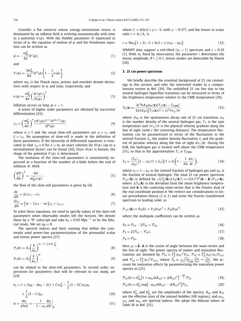
Table 1Uncertainties on slow-roll parameters for models classified according to the size of ε . The fiducial values at the time of horizon-crossing are chosen to be consistent withthe 2σ ranges favored by WMAP5 data [1].

Model Fiducial 1σ (Planck alone) 1σ (SKA + Planck) 1σ (FFTT + Planck)

High ε

1 parameter, ε 0.0071 6.9 × 10−4 6.3 × 10−4 6.9 × 10−5

2 parameter, ε 0.0053 0.0014 0.0014 0.0012η −0.013 0.0034 0.0033 0.0026

3 parameter, ε 0.0063 0.0015 0.0015 0.0014η 0.0069 0.0036 0.0033 0.0028ξ 0.00083 0.0026 0.0016 1.6 × 10−4

Low ε

2 parameter, ε 10−8 – – –η −0.027 0.0016 0.0014 1.5 × 10−4

3 parameter, ε 10−8 – – –η −0.0069 0.0024 0.0016 2.2 × 10−4

ξ 0.002 0.0026 0.0016 1.4 × 10−4

Fig. 1. 2σ forecasts for the fiducial points in Table 1 from a Fisher matrix analysis of SKA + Planck (dashed) and FFTT + Planck (solid) in the (n , r) and (n ,α) planes.

s s

Fsr =(

∂λspec

∂λsr

)T

Fspec∂λspec

∂λsr. (22)

The three independent spectral parameters allow the Jacobian ma-trix a maximal rank of three, and directly constrain up to threeslow-roll parameters. We consider Planck and 21 cm data inde-pendently, so the combined Fisher matrix is the sum of the contri-butions,

Ftotsr = F21 cm

sr + FPlancksr , (23)

which we use to construct a χ2 function,

χ2(λsr) = δTλsr

Ftotsr δλsr , (24)

where δ denotes the deviations from the fiducial values of theslow-roll parameters.

6. Results

We forecast constraints on the slow-roll parameters at the fidu-cial points of Table 1 that are consistent with WMAP5 results.To supplement the uncertainties listed in the table, we providethe corresponding (approximate) uncertainties for the more famil-iar spectral parameters. The joint SKA + Planck (FFTT + Planck)analysis gives the 1σ uncertainties δns = 0.0031, δα = 0.0032(δns = 6×10−4, δα = 2.7×10−4). These results roughly apply to allthe classes of models in Section 4. These uncertainties are larger,but consistent with those in Ref. [21] since we marginalize overall other parameters, while in Ref. [21], r and α are held fixed in

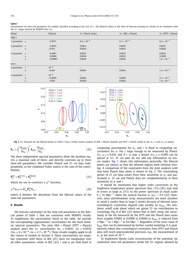
computing uncertainties for ns , and r is fixed in computing un-certainties for α. For r large enough to be measured by Planck,δr|r∼0.1 = 0.022 and if r is tiny, a bound δr|r∼0 = 0.005 can beplaced at 1σ . 21 cm data do not add any information on ten-sor modes. Fig. 1 shows this information pictorially. The fiducialpoints are chosen so that the allowed regions have minimal over-lap. A comparison of the constraints from the joint analyses withthat from Planck data alone is shown in Fig. 2. The constrainingpower of 21 cm data comes from their sensitivity to ns and par-ticularly α. 21 cm and Planck data are complementarity in theirsensitivity to α and r.

It should be mentioned that higher order corrections to thebrightness temperature power spectrum (Eqs. (15)–(20)) may leadto errors as large as O(1) in the power spectrum at small scalesk � 1h Mpc−1 when the neutral fraction is 〈xH 〉 ∼ 0.5 [22]. How-ever, since interferometer array measurements are more sensitiveto small k modes than to large k modes because of thermal noise,cosmological constraints depend only weakly on kmax, the non-linear cutoff scale above which we ignore 21 cm contributions tocosmology. Fig. 6 of Ref. [21] shows that in their setup, the uncer-tainty in the tilt measured by the FFTT and the Planck data variesfrom roughly 0.0003 to 0.0006 to 0.0009 as kmax is reduced from2 Mpc−1 to 1 Mpc−1 to 0.6 Mpc−1. Regardless of the exact value ofkmax that can be determined by further careful modeling, it is qual-itatively robust that cosmological constraints from FFTT and Planckdata will reach unprecedented precision, e.g., the measurement ofns at the level of 10−4.

To implement Monte Carlo reconstruction of the potential, werandomize slow-roll parameters inside the 2σ regions allowed by

V. Barger et al. / Physics Letters B 673 (2009) 173–178 177

21 cm + Planck data as the values when the scale k0 left the hori-zon. We then evolve Eqs. (6) and (7) forward in time. Those casesare selected in which inflation ends with the number of e-folds Nthat pass a prior Nmin < N < Nmax. The prior on N is necessary be-cause (i) a sufficiently large N is required to be consistent with theobserved horizon size; (ii) a small N indicates relatively fast rollingwhich suggests that higher-order parameters may not be smallenough to be truncated; (iii) a large N indicates that rolling is ex-tremely slow so that a hybrid mechanism might be responsible for

Fig. 2. The impact of 21 cm experiments on parameter estimation. 2σ regions froman analysis of Planck alone, 21 cm alone, and 21 cm + Planck. The fiducial point forthe high ε two-parameter model is used. FFTT and Planck are complementary: FFTThas good sensitivity to α but no sensitivity to r and Planck has good sensitivity tor but not α. We do not show the FFTT + Planck ellipse since it is indistinguishablefrom the ellipse for FFTT alone.

end the inflation. While our framework supposes that observableinflation is dominated by a single scalar field, it does not precludethe possibility of a hybrid transition caused by other fields endinginflation. We use two priors, 40 < N < 70 and 30 < N < 500. Thefirst prior is typical for a plausible expansion history of our uni-verse with Ref. [35] arguing for N between 50 and 60. This firstprior does not account for a hybrid transition. Our second prior israther conservative 30 < N < 500, with the large values suggestingthat some other mechanism brings an abrupt end to inflation.

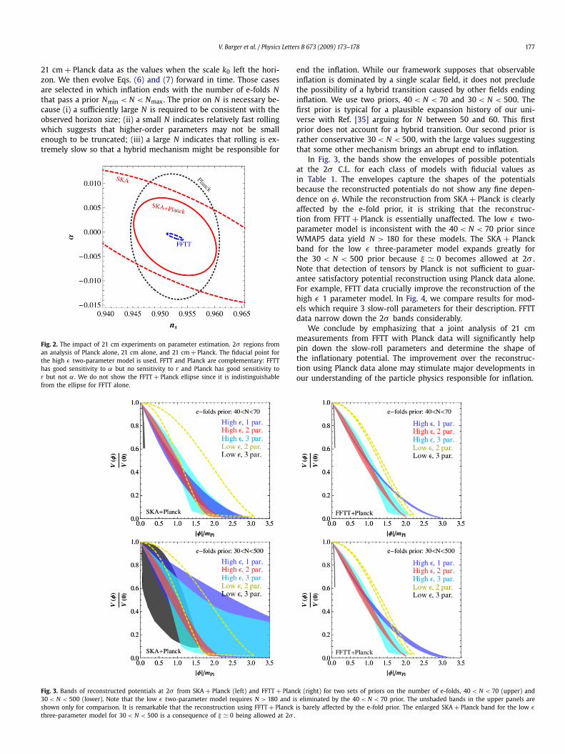
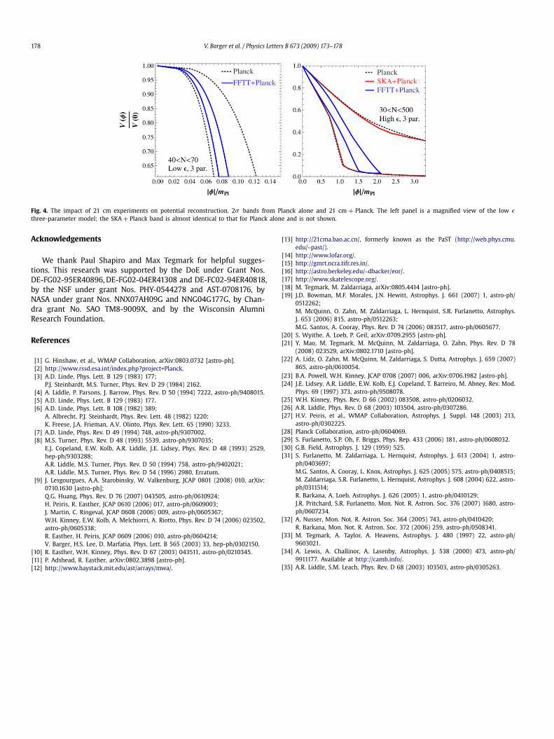
In Fig. 3, the bands show the envelopes of possible potentialsat the 2σ C.L. for each class of models with fiducial values asin Table 1. The envelopes capture the shapes of the potentialsbecause the reconstructed potentials do not show any fine depen-dence on φ. While the reconstruction from SKA + Planck is clearlyaffected by the e-fold prior, it is striking that the reconstruc-tion from FFTT + Planck is essentially unaffected. The low ε two-parameter model is inconsistent with the 40 < N < 70 prior sinceWMAP5 data yield N > 180 for these models. The SKA + Planckband for the low ε three-parameter model expands greatly forthe 30 < N < 500 prior because ξ � 0 becomes allowed at 2σ .Note that detection of tensors by Planck is not sufficient to guar-antee satisfactory potential reconstruction using Planck data alone.For example, FFTT data crucially improve the reconstruction of thehigh ε 1 parameter model. In Fig. 4, we compare results for mod-els which require 3 slow-roll parameters for their description. FFTTdata narrow down the 2σ bands considerably.

We conclude by emphasizing that a joint analysis of 21 cmmeasurements from FFTT with Planck data will significantly helppin down the slow-roll parameters and determine the shape ofthe inflationary potential. The improvement over the reconstruc-tion using Planck data alone may stimulate major developments inour understanding of the particle physics responsible for inflation.

Fig. 3. Bands of reconstructed potentials at 2σ from SKA + Planck (left) and FFTT + Planck (right) for two sets of priors on the number of e-folds, 40 < N < 70 (upper) and30 < N < 500 (lower). Note that the low ε two-parameter model requires N > 180 and is eliminated by the 40 < N < 70 prior. The unshaded bands in the upper panels areshown only for comparison. It is remarkable that the reconstruction using FFTT + Planck is barely affected by the e-fold prior. The enlarged SKA + Planck band for the low εthree-parameter model for 30 < N < 500 is a consequence of ξ � 0 being allowed at 2σ .

178 V. Barger et al. / Physics Letters B 673 (2009) 173–178

Fig. 4. The impact of 21 cm experiments on potential reconstruction. 2σ bands from Planck alone and 21 cm + Planck. The left panel is a magnified view of the low εthree-parameter model; the SKA + Planck band is almost identical to that for Planck alone and is not shown.

Acknowledgements

We thank Paul Shapiro and Max Tegmark for helpful sugges-tions. This research was supported by the DoE under Grant Nos.DE-FG02-95ER40896, DE-FG02-04ER41308 and DE-FC02-94ER40818,by the NSF under grant Nos. PHY-0544278 and AST-0708176, byNASA under grant Nos. NNX07AH09G and NNG04G177G, by Chan-dra grant No. SAO TM8-9009X, and by the Wisconsin AlumniResearch Foundation.

References

[1] G. Hinshaw, et al., WMAP Collaboration, arXiv:0803.0732 [astro-ph].[2] http://www.rssd.esa.int/index.php?project=Planck.[3] A.D. Linde, Phys. Lett. B 129 (1983) 177;

P.J. Steinhardt, M.S. Turner, Phys. Rev. D 29 (1984) 2162.[4] A. Liddle, P. Parsons, J. Barrow, Phys. Rev. D 50 (1994) 7222, astro-ph/9408015.[5] A.D. Linde, Phys. Lett. B 129 (1983) 177.[6] A.D. Linde, Phys. Lett. B 108 (1982) 389;

A. Albrecht, P.J. Steinhardt, Phys. Rev. Lett. 48 (1982) 1220;K. Freese, J.A. Frieman, A.V. Olinto, Phys. Rev. Lett. 65 (1990) 3233.

[7] A.D. Linde, Phys. Rev. D 49 (1994) 748, astro-ph/9307002.[8] M.S. Turner, Phys. Rev. D 48 (1993) 5539, astro-ph/9307035;

E.J. Copeland, E.W. Kolb, A.R. Liddle, J.E. Lidsey, Phys. Rev. D 48 (1993) 2529,hep-ph/9303288;A.R. Liddle, M.S. Turner, Phys. Rev. D 50 (1994) 758, astro-ph/9402021;A.R. Liddle, M.S. Turner, Phys. Rev. D 54 (1996) 2980, Erratum.

[9] J. Lesgourgues, A.A. Starobinsky, W. Valkenburg, JCAP 0801 (2008) 010, arXiv:0710.1630 [astro-ph];Q.G. Huang, Phys. Rev. D 76 (2007) 043505, astro-ph/0610924;H. Peiris, R. Easther, JCAP 0610 (2006) 017, astro-ph/0609003;J. Martin, C. Ringeval, JCAP 0608 (2006) 009, astro-ph/0605367;W.H. Kinney, E.W. Kolb, A. Melchiorri, A. Riotto, Phys. Rev. D 74 (2006) 023502,astro-ph/0605338;R. Easther, H. Peiris, JCAP 0609 (2006) 010, astro-ph/0604214;V. Barger, H.S. Lee, D. Marfatia, Phys. Lett. B 565 (2003) 33, hep-ph/0302150.

[10] R. Easther, W.H. Kinney, Phys. Rev. D 67 (2003) 043511, astro-ph/0210345.[11] P. Adshead, R. Easther, arXiv:0802.3898 [astro-ph].[12] http://www.haystack.mit.edu/ast/arrays/mwa/.

[13] http://21cma.bao.ac.cn/, formerly known as the PaST (http://web.phys.cmu.edu/~past/).

[14] http://www.lofar.org/.[15] http://gmrt.ncra.tifr.res.in/.[16] http://astro.berkeley.edu/~dbacker/eor/.[17] http://www.skatelescope.org/.[18] M. Tegmark, M. Zaldarriaga, arXiv:0805.4414 [astro-ph].[19] J.D. Bowman, M.F. Morales, J.N. Hewitt, Astrophys. J. 661 (2007) 1, astro-ph/

0512262;M. McQuinn, O. Zahn, M. Zaldarriaga, L. Hernquist, S.R. Furlanetto, Astrophys.J. 653 (2006) 815, astro-ph/0512263;M.G. Santos, A. Cooray, Phys. Rev. D 74 (2006) 083517, astro-ph/0605677.

[20] S. Wyithe, A. Loeb, P. Geil, arXiv:0709.2955 [astro-ph].[21] Y. Mao, M. Tegmark, M. McQuinn, M. Zaldarriaga, O. Zahn, Phys. Rev. D 78

(2008) 023529, arXiv:0802.1710 [astro-ph].[22] A. Lidz, O. Zahn, M. McQuinn, M. Zaldarriaga, S. Dutta, Astrophys. J. 659 (2007)

865, astro-ph/0610054.[23] B.A. Powell, W.H. Kinney, JCAP 0708 (2007) 006, arXiv:0706.1982 [astro-ph].[24] J.E. Lidsey, A.R. Liddle, E.W. Kolb, E.J. Copeland, T. Barreiro, M. Abney, Rev. Mod.

Phys. 69 (1997) 373, astro-ph/9508078.[25] W.H. Kinney, Phys. Rev. D 66 (2002) 083508, astro-ph/0206032.[26] A.R. Liddle, Phys. Rev. D 68 (2003) 103504, astro-ph/0307286.[27] H.V. Peiris, et al., WMAP Collaboration, Astrophys. J. Suppl. 148 (2003) 213,

astro-ph/0302225.[28] Planck Collaboration, astro-ph/0604069.[29] S. Furlanetto, S.P. Oh, F. Briggs, Phys. Rep. 433 (2006) 181, astro-ph/0608032.[30] G.B. Field, Astrophys. J. 129 (1959) 525.[31] S. Furlanetto, M. Zaldarriaga, L. Hernquist, Astrophys. J. 613 (2004) 1, astro-

ph/0403697;M.G. Santos, A. Cooray, L. Knox, Astrophys. J. 625 (2005) 575, astro-ph/0408515;M. Zaldarriaga, S.R. Furlanetto, L. Hernquist, Astrophys. J. 608 (2004) 622, astro-ph/0311514;R. Barkana, A. Loeb, Astrophys. J. 626 (2005) 1, astro-ph/0410129;J.R. Pritchard, S.R. Furlanetto, Mon. Not. R. Astron. Soc. 376 (2007) 1680, astro-ph/0607234.

[32] A. Nusser, Mon. Not. R. Astron. Soc. 364 (2005) 743, astro-ph/0410420;R. Barkana, Mon. Not. R. Astron. Soc. 372 (2006) 259, astro-ph/0508341.

[33] M. Tegmark, A. Taylor, A. Heavens, Astrophys. J. 480 (1997) 22, astro-ph/9603021.

[34] A. Lewis, A. Challinor, A. Lasenby, Astrophys. J. 538 (2000) 473, astro-ph/9911177. Available at http://camb.info/.

[35] A.R. Liddle, S.M. Leach, Phys. Rev. D 68 (2003) 103503, astro-ph/0305263.