Embed Size (px)
Citation preview
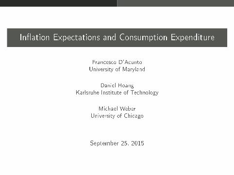
In�ation Expectations and Consumption Expenditure
Francesco D'Acunto
University of Maryland
Daniel Hoang
Karlsruhe Institute of Technology
Michael Weber
University of Chicago
September 25, 2015

Introduction
Research Question
Do higher in�ation expectations lead to higher consumption?
Monetary policy constrained when zero lower bound (ZLB) binds
Higher in�ation expectations lower real interest rates with binding ZLB
Fiscal multipliers increase with higher in�ation when ZLB binds
But: precautionary savings channel, preference assumptions, in�ation
tax on liquid asset, income e�ects, etc.
⇒ Relationship in�ation expectations ⇔ consumption empirical question

Introduction
This Paper
Relationship btw in�ation expectations & willingness to purchase
Use novel German household data for sample Jan 2000 to Dec 2013
Unexpected rise in value-added tax as shock to in�ation expectations
Match German & foreign HHs in DiD research design for identi�cation
Main �nding: Households which expect in�ation to increase 9% more
likely to purchase durables
E�ect stronger for more educated, high-income, urban households

Introduction
Overview of Results: Time-Series Evidence
2005m11
2005m12
2006m1
2006m2
2006m3
2006m4
2006m52006m6
2006m7
2006m8
2006m9 2006m10
2006m11
2006m121.
61.
82
2.2
2.4
Goo
d tim
e to
buy
Dur
able
s
0 .1 .2 .3 .4 .5Fraction inflation increases
HH with positive in�ation expectations 9% more likely to purchase durables in XS
19% after announcement and before taking e�ect of VAT (11/05 � 12/06): blue dots

Introduction
Related Literature
Theoretical literature on stabilization role of in�ation
Monetary policy: Krugman (1998), Eggertsson, Woodford (2003),Eggertsson (2006), Werning (2012)
Fiscal policy: Eggertsson (2011), Christiano, Eichenbaum, Rebelo(2001), Woodford (2011)
Historical perspective: Romer, Romer (2013), Eggertsson (2008)
Household survey data on in�ation expectations
Bachmann, Berg, Sims (2015), Burke, Ozdagli (2013), Ichiue,Nishiguchi (2015), Carvalho, Necchio (2014), Binder (2015)
Data
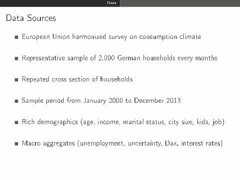
Data Sources
European Union harmonized survey on consumption climate
Representative sample of 2,000 German households every months
Repeated cross section of households
Sample period from January 2000 to December 2013
Rich demographics (age, income, marital status, city size, kids, job)
Macro aggregates (unemployment, uncertainty, Dax, interest rates)

Data
Survey Questions I
Question 8
Given the current economic situation, do you think it's a good time for your
households to buy larger items such as furniture, electronic items, etc.?
Answer choices: �it's neither good nor bad time,� �it's bad time,� or �it's a good time.�

Data
Survey Questions II
Question 3
How will consumer prices evolve during the next twelve months compared
to the previous twelve months?
Answer choices: �prices will increase more,� �prices will increase by the same,� �prices
will increase less,� �prices will stay the same,� or �prices will decrease.�
Create a dummy that equals 1 when households answer �prices will increase more.�

Data
In�ation Expectations over time
0
0.1
0.2
0.3
0.4
0.5
12/0
012
/01
12/0
212
/03
12/0
412
/05
12/0
612
/07
12/0
812
/09
12/1
012
/11
12/1
212
/13
FractionInflationIncreases
In�ation expectation start building up beginning of 2006
Spike in December of 2006

Data
Durable In�ation and lagged In�ation Expectations
−2
−1
0
1
2
3
4
5
StandardizedInflation
12/0
112
/02
12/0
312
/04
12/0
512
/06
12/0
712
/08
12/0
912
/10
12/1
112
/12
12/1
3
Standardized Lagged Inflation ExpectationsStandardized Durable Inflation
Increase in CPI in�ation in 2007 driven by durable goods in�ation subject to VAT increase
Lagged in�ation expectations and standardized durable in�ation highly correlated
Data
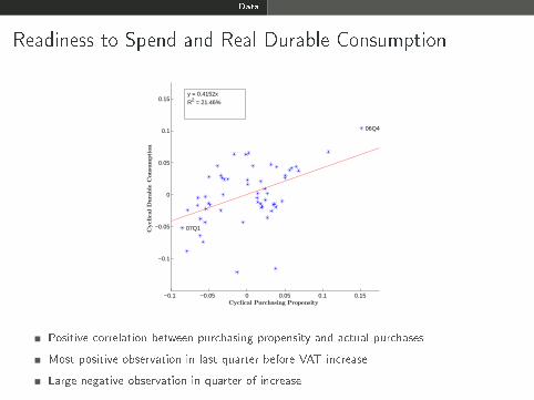
Readiness to Spend and Real Durable Consumption
−0.1 −0.05 0 0.05 0.1 0.15
−0.1
−0.05
0
0.05
0.1
0.15
Cyclical Purchasing Propensity
CyclicalDurable
Consumption
06Q4
07Q1
y = 0.4152xR2 = 21.46%
Positive correlation between purchasing propensity and actual purchases
Most positive observation in last quarter before VAT increase
Large negative observation in quarter of increase

Econometric Model
Baseline Speci�cation: Multinomial Logit
Assume survey answer is random variable y
De�ne the response probabilities as P(y = t|X )
X contains unit vector, and a rich set of household-level observables
Assume the distribution of the response probabilities is
P(y = t|X ) =eXβt
1+∑
z=1,2 eXβz
,
Estimate βt via maximum likelihood
Marginal e�ect: derivative of P(y = t|x) with respect to x

Empirical Results
Baseline Speci�cation
Marginal E�ects:∂P(y = t|x)
∂x= P(y = t|x)
βtx − ∑z=0,1,2
P(y = z|x)βzx
Bad time Good time Bad time Good time
(1) (2) (3) (4)
In�ation Increase 4.61∗∗∗ 6.24∗∗∗ 2.25 ∗ ∗ 7.49∗∗∗(1.09) (1.62) (0.91) (1.52)
Past In�ation 6.32∗∗∗ −3.42∗∗∗(0.48) (0.28)
Pseudo R2 0.0031 0.0161
Nobs 326,011 321,496
Households which expect in�ation to increase
7% more likely to answer �good time to purchase durables�
BUT also 2% to 4.5% more likely to reply �bad time to purchase durables�
Empirical Results
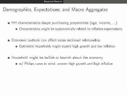
Demographics, Expectations, and Macro Aggregates
HH characteristics shape purchasing propensities (age, income, ...)
Characteristics might be systematically related to in�ation expectations
Economic outlook can a�ect cross-sectional relationship
Optimistic households might expect high growth and low in�ation
Household might be bullish or bearish about the economy
w/ Philips curve in mind: answer high growth and high in�ation

Empirical Results
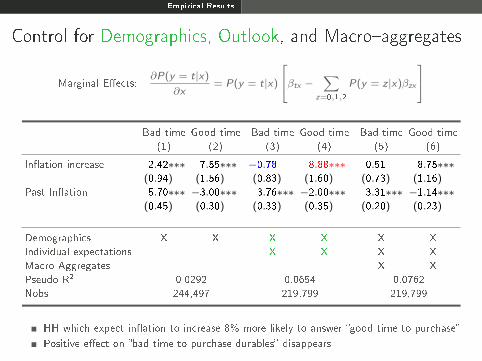
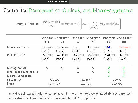
Control for Demographics, Outlook, and Macro�aggregates
Marginal E�ects:∂P(y = t|x)
∂x= P(y = t|x)
βtx − ∑z=0,1,2
P(y = z|x)βzx
Bad time Good time Bad time Good time Bad time Good time
(1) (2) (3) (4) (5) (6)
In�ation increase 2.42∗∗∗ 7.55∗∗∗ −0.78 8.88∗∗∗ 0.51 8.75∗∗∗(0.94) (1.56) (0.83) (1.60) (0.73) (1.16)
Past In�ation 5.70∗∗∗ −3.00∗∗∗ 3.76∗∗∗ −2.00∗∗∗ 3.31∗∗∗ −1.14∗∗∗(0.45) (0.30) (0.33) (0.35) (0.20) (0.23)
Demographics X X X X X X
Individual expectations X X X X
Macro Aggregates X X
Pseudo R2 0.0292 0.0654 0.0762
Nobs 244,497 219,799 219,799
HH which expect in�ation to increase 8% more likely to answer �good time to purchase�
Positive e�ect on �bad time to purchase durables� disappears
Empirical Results
Control for Demographics, Outlook, and Macro�aggregates
Marginal E�ects:∂P(y = t|x)
∂x= P(y = t|x)
βtx − ∑z=0,1,2
P(y = z|x)βzx
Bad time Good time Bad time Good time Bad time Good time
(1) (2) (3) (4) (5) (6)
In�ation increase 2.42∗∗∗ 7.55∗∗∗ −0.78 8.88∗∗∗ 0.51 8.75∗∗∗(0.94) (1.56) (0.83) (1.60) (0.73) (1.16)
Past In�ation 5.70∗∗∗ −3.00∗∗∗ 3.76∗∗∗ −2.00∗∗∗ 3.31∗∗∗ −1.14∗∗∗(0.45) (0.30) (0.33) (0.35) (0.20) (0.23)
Demographics X X X X X X
Individual expectations X X X X
Macro Aggregates X X
Pseudo R2 0.0292 0.0654 0.0762
Nobs 244,497 219,799 219,799
HH which expect in�ation to increase 8% more likely to answer �good time to purchase�
Positive e�ect on �bad time to purchase durables� disappears

Empirical Results
Individual Economic Outlook
Marginal E�ects:∂P(y = t|x)
∂x= P(y = t|x)
βtx − ∑z=0,1,2
P(y = z|x)βzx
Higher growth outlook Lower growth outlook
Bad time Good time Bad time Good time
(1) (2) (3) (4)
In�ation increase −0.58 8.41∗∗∗ 2.89∗∗∗ 7.29∗∗∗(1.15) (1.91) (0.90) (1.42)
Past In�ation 4.77∗∗∗ −3.55∗∗∗ 6.57∗∗∗ −3.20∗∗∗(0.49) (0.38) (0.47) (0.28)
Demographics X X X X
Individual expectations X X
Pseudo R2 0.0115 0.0171
Nobs 70,000 251,496
HH which expect in�ation to increase 8% more likely to answer �good time to purchase�
Positive e�ect on �bad time to purchase� contained among HH with negative outlook

Empirical Results
Exogenous Shock to In�ation Expectations
Richness of micro data many desirable features
BUT: cannot rule out movements along the supply curve
Here: expected in�ation and propensity to buy mitigates concern
Ideal experiment: shock to in�ation expectations that does not a�ect
households' willingness to purchase durables through channels
di�erent from expectations of rising prices
Follow narrative approach of Romer and Romer (2010)
⇒ Unexpected increase in value-added tax (VAT)
Empirical Results
VAT Experiment of 2007 I
Nov 2005: new government announces increase in VAT by 3%
Jan 2007: entry into force of VAT increase
Pre-election: promise not to increase VAT
VAT increase legislated to consolidate budget
Not related to prospective economic conditions
Exogenous tax change acc to Romer and Romer nomenclature
Empirical Results
VAT Experiment of 2007 II
In�ation expectations build up during 2006
Germany part of Euro zone and no independent monetary policy
Nominal rate did not increase to o�set in�ation expectations
Experiment resembles unconventional �scal policy described in
Correira, Fahri, Nicolini, Teles (2013)
Feldstein (2002) proposition for Japan: Pre-announced VAT increases
Stimulate in�ation expectations & private spending

Empirical Results
VAT as Shock to In�ation Expectations
12/0
012
/01
12/0
212
/03
12/0
412
/05
12/0
612
/07
12/0
812
/09
12/1
012
/11
12/1
212
/13
Fra
ctio
nIn.ati
on
Incr
ease
s
0
0.1
0.2
0.3
0.4
0.5
Announcement Increase
In�ation expectation start building up beginning of 2006
Spike in December of 2006
Empirical Results
Di�erence-in-Di�erences Matching Estimator
All Germans treated by VAT shocks
Micro data for France, UK, Sweden from EU harmonized survey
Match German & foreign households with nearest-neighbor algorithm
Matching categories: gender, age, education, income, social status
Estimate Average Treatment E�ect of VAT shock:
(DurGerman,post − DurGerman,pre)− (Dur foreign,post − Dur foreign,pre)

Empirical Results
Parallel-Trends Identi�cation Assumption I
Control group behaves similarly to Germans before VAT shock
Behavior of control group after shock how Germans behaved absent of it
Empirical Results
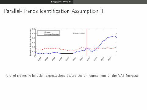
Parallel-Trends Identi�cation Assumption II
03/0
406
/04
09/0
412
/04
03/0
506
/05
09/0
512
/05
03/0
606
/06
09/0
6
Fra
ctio
nIn.ati
on
Incr
ease
s
0
0.1
0.2
0.3
0.4
0.5
0.6
AnnouncementGermanyEuropean Countries
Parallel trends in in�ation expectations before the announcement of the VAT increase
Empirical Results
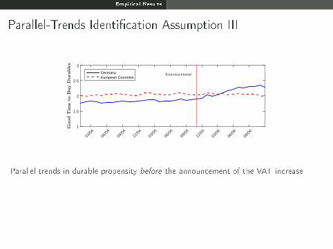
Parallel-Trends Identi�cation Assumption III
03/0
406
/04
09/0
412
/04
03/0
506
/05
09/0
512
/05
03/0
606
/06
09/0
6
Good
Tim
eto
Buy
Dura
ble
s
1
1.5
2
2.5
3
AnnouncementGermanyEuropean Countries
Parallel trends in durable propensity before the announcement of the VAT increase
Empirical Results
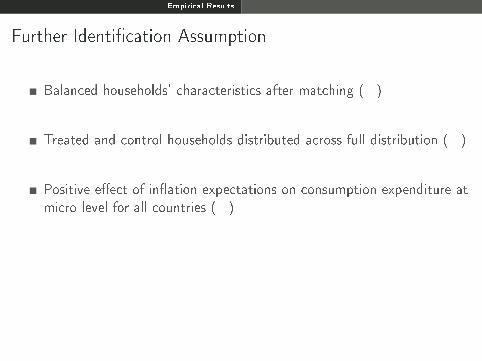
Further Identi�cation Assumption
Balanced households' characteristics after matching (√)
Treated and control households distributed across full distribution (√)
Positive e�ect of in�ation expectations on consumption expenditure at
micro level for all countries (√)

Empirical Results
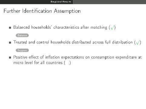
Further Identi�cation Assumption
Balanced households' characteristics after matching (√)
Balance
Treated and control households distributed across full distribution (√)
Positive e�ect of in�ation expectations on consumption expenditure at
micro level for all countries (√)
Empirical Results
Further Identi�cation Assumption
Balanced households' characteristics after matching (√)
Balance
Treated and control households distributed across full distribution (√)
Support
Positive e�ect of in�ation expectations on consumption expenditure at
micro level for all countries (√)
Empirical Results
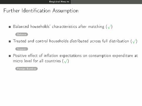
Further Identi�cation Assumption
Balanced households' characteristics after matching (√)
Balance
Treated and control households distributed across full distribution (√)
Support
Positive e�ect of in�ation expectations on consumption expenditure at
micro level for all countries (√)
Foreign Baseline

Empirical Results
Average Treatment E�ect of VAT shock
(DurGerman,post − DurGerman,pre)− (Dur foreign,post − Dur foreign,pre)
09/0
512
/05
03/0
606
/06
09/0
612
/06
03/0
706
/07
09/0
7
Avera
ge
Tre
atm
ent
E,ect
-0.1
-0.05
0
0.05
0.1
0.15
0.2
0.25
0.3
0.35
0.4
Average Treatment Effect Over TimeTwo-Standard Error Bounds
German and foreign households behave similarly before shock
Immediate increase of purchasing behavior of Germans after shock
E�ect builds up during 2006
Reversion to normal after actual VAT increase
Empirical Results
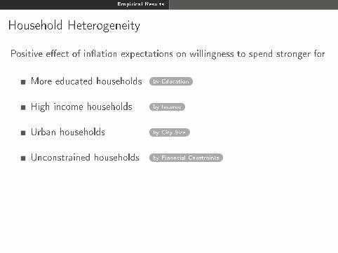
Household Heterogeneity
Positive e�ect of in�ation expectations on willingness to spend stronger for
More educated households by Education
High income households by Income
Urban households by City Size
Unconstrained households by Financial Constraints
Empirical Results
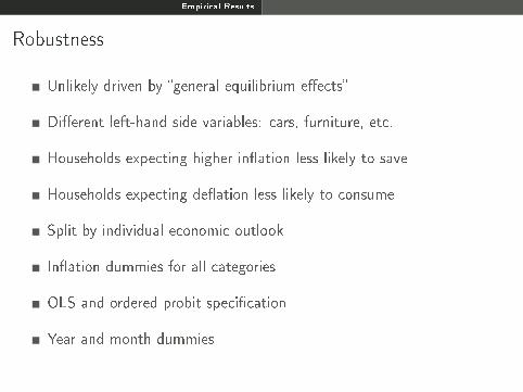
Robustness
Unlikely driven by �general equilibrium e�ects�
Di�erent left-hand side variables: cars, furniture, etc.
Households expecting higher in�ation less likely to save
Households expecting de�ation less likely to consume
Split by individual economic outlook
In�ation dummies for all categories
OLS and ordered probit speci�cation
Year and month dummies
Empirical Results
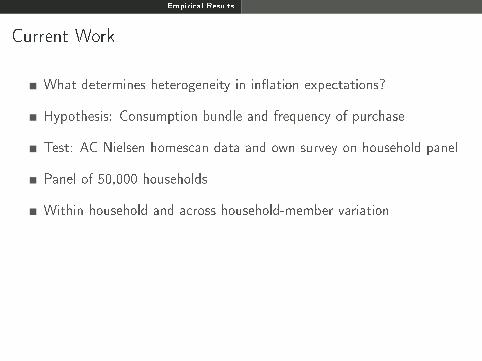
Current Work
What determines heterogeneity in in�ation expectations?
Hypothesis: Consumption bundle and frequency of purchase
Test: AC Nielsen homescan data and own survey on household panel
Panel of 50,000 households
Within household and across household-member variation

Empirical Results
Conclusion
We document a positive cross-sectional relationship between
households' in�ation expectation and their willingness to purchase
durable goods
The positive e�ect is stronger for more educated, urban, working-age,
and higher income households
Our �ndings provide support for conventional wisdom that temporarily
higher in�ation expectations can stir consumption expenditure
The heterogeneity across households and the delayed response in 2006
suggest scope for increased economic literacy and policy transparency
Discretionary �scal policy in recessions: series of pre-announced VAT
increases and a simultaneous Freduction in income tax rates
Appendix
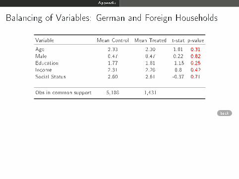
Balancing of Variables: German and Foreign Households
Variable Mean Control Mean Treated t-stat p-value
Age 2.33 2.30 1.01 0.31
Male 0.47 0.47 0.22 0.82
Education 1.77 1.81 -1.15 0.25
Income 2.31 2.28 0.8 0.42
Social Status 2.60 2.61 -0.37 0.71
Obs in common support 5,108 1,431
back

Appendix
Balancing of Variables: German and Foreign Households
0 .2 .4 .6 .8Propensity Score
Untreated Treated
back

Appendix
Baseline Speci�cation Foreign Households
France Sweden UK
(1) (2) (3)
In�ation Increase 2.65∗∗∗ 3.81∗∗∗ 4.65∗∗∗(0.37) (0.53) (0.61)
Past In�ation −1.63∗∗∗ −3.15∗∗∗ −0.61(0.15) (0.55) (0.19)
Demographics X X X
Individual expectations X X X
Pseudo R2 0.0445 0.0288 0.0508
Nobs 163,419 176,829 113,774
Standard errors in parentheses
∗p < 0.10, ∗ ∗ p < 0.05, ∗ ∗ ∗p < 0.01
back

Appendix
Baseline Speci�cation by Education
Marginal E�ects:∂P(y = t|x)
∂x= P(y = t|x)
βtx − ∑z=0,1,2
P(y = z|x)βzx
Hauptschule Realschule Gymnasium University
Bad time Good time Bad time Good time Bad time Good time Bad time Good time
(1) (2) (3) (4) (5) (6) (7) (8)
In�ation increase 1.08 6.89∗∗∗ 1.17 9.85∗∗∗ −3.42∗∗∗ 9.79∗∗∗ −3.87∗∗∗ 11.28∗∗∗(1.05) (1.52) (0.80) (1.62) (1.18) (2.25) (0.80) (1.88)
Past In�ation 4.14∗∗∗ −1.94∗∗∗ 3.73∗∗∗ −1.88∗∗∗ 3.19∗∗∗ −2.64∗∗∗ 2.52∗∗∗ −2.14∗∗∗(0.34) (0.32) (0.34) (0.38) (0.47) (0.48) (0.45) (0.57)
Demographics X X X X X X X X
Individual expectations X X X X X X X X
Pseudo R2 0.0673 0.0635 0.0415 0.0508
Nobs 89,991 88,315 23,282 18,211
back

Appendix
Baseline Speci�cation by Income
Marginal E�ects:∂P(y = t|x)
∂x= P(y = t|x)
βtx − ∑z=0,1,2
P(y = z|x)βzx
Income ≤ 1,000 1,000 < Income ≤ 2,500 2,500 < Income
Bad time Good time Bad time Good time Bad time Good time
(1) (2) (3) (4) (5) (6)
In�ation increase −0.99 8.98∗∗∗ −0.55 8.51∗∗∗ −1.09 10.48∗∗∗(1.05) (1.68) (0.78) (1.51) (0.77) (2.03)
Past In�ation 4.23∗∗∗ −1.94∗∗∗ 3.51∗∗∗ −1.92∗∗∗ 2.77∗∗∗ −2.99∗∗∗(0.36) (0.37) (0.32) (0.36) (0.43) (0.45)
Demographics X X X X X X
Individual expectations X X X X X X
Pseudo R2 0.0655 0.0596 0.0504
Nobs 96,555 112,710 16,477
back

Appendix
Baseline Speci�cation by City Size
Marginal E�ects:∂P(y = t|x)
∂x= P(y = t|x)
βtx − ∑z=0,1,2
P(y = z|x)βzx
City ≤ 2T 2T < City ≤ 20T 20T < City ≤ 100T 100T < City
Bad time Good time Bad time Good time Bad time Good time Bad time Good time
(1) (2) (3) (4) (5) (6) (7) (8)
In�ation increase −1.23 5.81∗∗∗ 0.18 8.47∗∗∗ 0.02 8.54∗∗∗ −2.44∗∗∗ 10.13∗∗∗(1.32) (1.99) (0.86) (1.51) (1.02) (2.17) (0.92) (1.33)
Past In�ation 4.14∗∗∗ −1.96∗∗∗ 2.98∗∗∗ −1.87∗∗∗ 4.14∗∗∗ −2.64∗∗∗ 4.15∗∗∗ −1.77∗∗∗(0.52) (0.55) (0.36) (0.34) (0.37) (0.38) (0.40) (0.42)
Demographics X X X X X X X X
Individual expectations X X X X X X X X
Pseudo R2 0.0738 0.0632 0.0721 0.0656
Nobs 17,833 74,937 59,674 67,355
Standard errors in parentheses
∗p < 0.10, ∗ ∗ p < 0.05, ∗ ∗ ∗p < 0.01
back

Appendix
Baseline Speci�cation by Financial Constraints
Marginal E�ects:∂P(y = t|x)
∂x= P(y = t|x)
βtx − ∑z=0,1,2
P(y = z|x)βzx
Unconstrained Constrained
Bad time Good time Bad time Good time
(1) (2) (3) (4)
In�ation Increase −0.57 10.42∗∗∗ −1.05 7.47∗∗∗(0.66) (1.80) (1.01) (1.46)
Past In�ation 3.45∗∗∗ −2.50∗∗∗ 3.88∗∗∗ −1.59∗∗∗(0.27) (0.38) (0.40) (0.35)
Pseudo R2 0.0615 0.0608
Nobs 98,344 121,455
back