Inflation and Unit Labor Cost

Robert G. KingMark W. Watson

Prepared for Studienzentrum Gerzensee25th anniversary conference

1

Familiar New Keynesian Price Equation

• Single equation (Gali & Gertler, Sbordonne)• Component of DSGE models (Smets and Wouters) • Link between inflation and real cost measure

• is real unit labor cost or modification of it indicated by particular production/market structure

• “z” is other factors, sometimes given a structural interpretation (such as price markup shocks in SW)

• NKPE provides a direct 4‐way breakdown (Decomposition #1) into inertia, expectations, cost, and residual

ttttftbt zE 11

2

Inflation and rulc[similar to Figure 6 in packet: internal validity sample period]

1960 1965 1970 1975 1980 1985 1990 1995 2000-5

0

5

10

15

Per

cent

per

yea

r, P

erce

nt d

evia

tion

Inflation and Real Unit Labor Cost

GDP inflationNFB real ULC

3

Evolving project:our starting questions

• What account do modern NK‐DSGE models provide about forces which drive inflation?– On average, during estimation period (60‐99)– During particular episodes– Before and afterward

• How does conclusion depend on whether one looks directly at NKPE or its rational expectation solution?

4

Why is NKPE attractive?

• Theoretical foundations (Calvo model)• Near neutrality with respect to inflation trends• Forward‐looking elements inevitable with sticky prices

• Empirically tractable• Real unit labor costs allows side‐step of difficult task of measuring capacity output in a world of changing technology

• Allows ready consideration of implications of alternative inflation targeting policies 

5

Decomposition 1: What are sources of inflation?Figure 10’s direct answer from NKPE 

using GG measure of parameters and cost

6

Conclusions from Decomposition #1• Inflation dominated by expectations• Small direct contribution of cost (which is sole channel 

for monetary policy and aggregate demand)• Not too much inflation inertia• Robust: parameters  (GG versus SW); cost measures (GG 

versus SW);  inflation forecasting (GG‐VAR, SW‐DSGE)• Robust to levels or deviations from trend (using 1‐sided 

HP filter to remove trend)• Inflation shocks are not dominant

7

Decomposition #2: Fundamental Inflation

• History It was precisely this type of decomposition in the work of Gali‐Gertler (1999) and Sbordonne (2002) that generated impetus toward NKPE in DSGE models. 

• Example of Interpretation of single equation or block of equations within a DSGE model. Focuses on inflation impact of DSGE modeling assumptions.– Our 1996 REStat study yielded disappointing results for an NKPE+DSGE framework

– It contained Calvo pricing w/o inflation inertia mechanism– But the rest of the DSGE was very different from SW: much simpler core neoclassical structure (e.g., no consumption habit) well as no nominal wage rigidity

8

Insert GG Figure 2

9

Figure 12: Replicating the potential displayed in  GGS

10

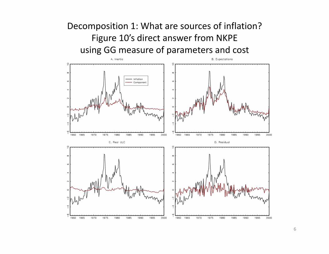
Decomposition #2:Mechanics of Fundamental Inflation 

(RE forward solution)

t

jjtt

jt

t

tt

zttt

dMIL

EL

d

11

0

1

1tt

][)1(

)1(

DSGE]or [VAR uMdd vectors]data ,[selection

11

Figure 18: Unexpected (to us) results in SW

12

Switching from accounting to diagnosisWhat are the candidates?

1. Parameters ()2. Measure of cost (3. Forecasting model (M)

a) 2 variable VAR in GGb) DSGE solution in SWc) Implied 2 variable VAR for SW (population 

approximation or empirical) 4. Various combinations of above: Fundamental 

inflation is complicated function of , M  so we’ll develop a simple approximation

13

14

Parameters in NKPE  

b f GG 0.25 0.68 0.153SW 0.19 0.81 0.082

Parameters in Fundamental Inflation

zGG 0.32 0.876 0.197 5.14

SW 0.23 0.998 0.101 4.91

Figure 15: Cost Measures

15

• Overhead corrections (model consistent) to rulc in SW, which we call modified unit labor cost (mulc) and some differences in data since they are modeling GDP rather than NFB

• Log indexes adjusted to common mean

More on cost differences

• Differences large in trend, smaller detrended• Irony: real unit labor cost has some similar issues to output gaps

16

Approximating Fundamental Inflation1. Estimate bivariate VAR (d=[

a) Just as in GGb) Simplification for SW

2. Use this VAR to form FI solution 

3. Sum the FI solution coefficients  on  and 4. Compute approximation  to as 

5. Approximation emphasizes trends

17

ttt )1( )1(~

tt dMIL 11 ][)1(

Figure 15: Approximation for GG fundamental inflation

18

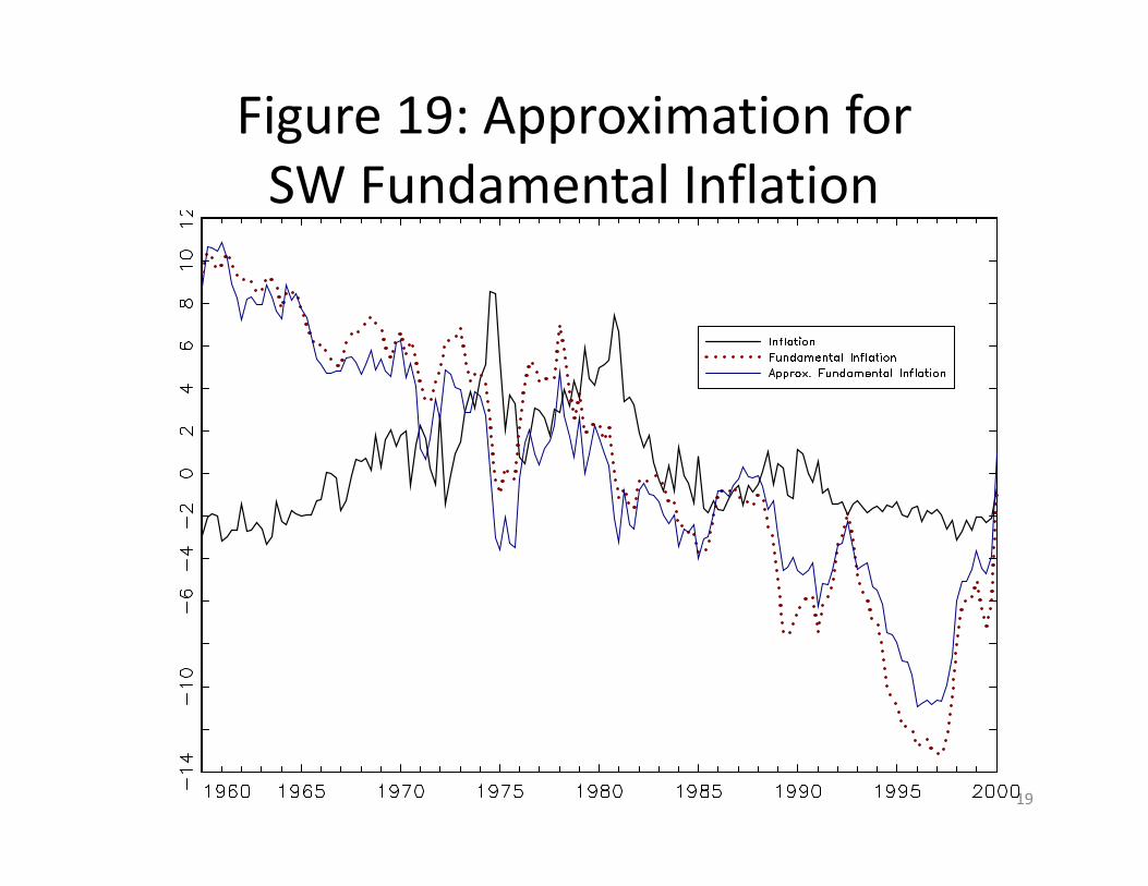
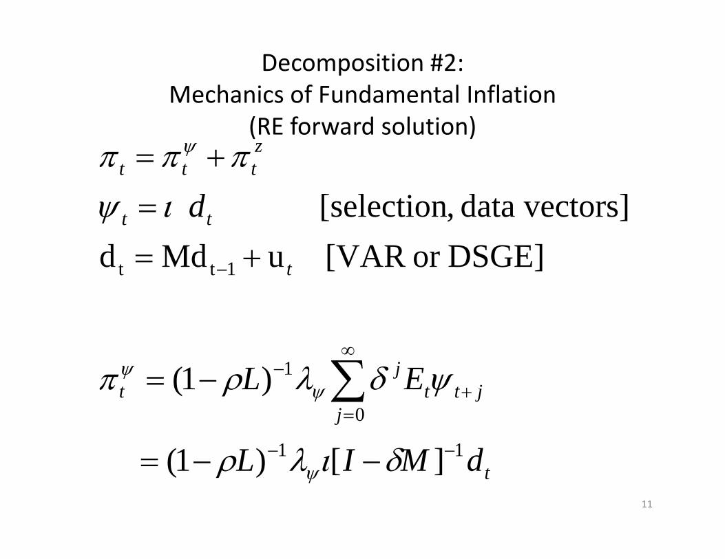
Figure 19: Approximation for SW Fundamental Inflation

19

Key findings

• Approximation is quite good • Parameters are not responsible for large differences between GG and SW

• Both approximating VAR thru beta and cost data help explain large differences 

• But the rest of the SW DSGE model is not the source of the puzzle: it fits the moments of the SW data quite well. 

• Robustness in table 5

20

Key findings from approximation (cont’d)

• GG fundamental inflation – places positive weight on both  and – Reference approximation for FI is .85 +.15 – Triangular shape  in “inflation trend” and downward “cost trend” yields main historical inflation patterns

• SW fundamental inflation – places bigger positive weight on measured cost and negative weight on actual inflation

– Reference approximation for FI is  1.45  ‐ .7 – Approximation closely captures puzzling picture, linking SW‐FI to trends in inflation and modified rulc

21

Inside the SW model

• Elements of their Historical Decompositions– As SW emphasize, structural wage and price markup shocks are the key drivers of inflation 

– But price markup shocks also are very important for SW marginal cost measure, which we are calling modified real unit labor cost (MRULC) 

22

Figure 7: SW inflation historical decomposition

23

Figure 8: SW cost historical decomposition

24

Four impulse responses

• Revision in inflation path due to structural price shock (z)

• Revision in present discounted value forecast z of structural price shock (same sign, larger)

• Revision in modified real unit labor cost (very persistent; offsetting z effect)

• Revision in fundamental inflation (opposite sign to z)

25

SW impulse responses forstructural shock, inflation and cost

26

SW model impulse responses for fundamental inflation and z

27

Why pattern in SW model?• Take 1: Price markup shock and inflation targeting pattern

– Would be “neutral” if just right “flexible inflation target” moves in z– Inflation shock z rises in a persistent manner (ARMA(1,1) with ar=.9 

and ma=.7) and discounted z rises as well (more than one‐for‐one)– Inflation  does not rise much (policy rule behind this…) and thus 

“fundamental inflation” must fall.

• Take 2:  Price markup shock and real activity pattern– The components of SW modified rulc (real wage, labor input, and 

output) all fall in response , but compensation falls by more than output principally due to real wage declines

– Real marginal cost is still roughly “inverse of markup” as in simpler models 

– there is a very slow equilibrating process for the wage and mrulcbecause the markup is very persistent (.9^12=.24) 

28

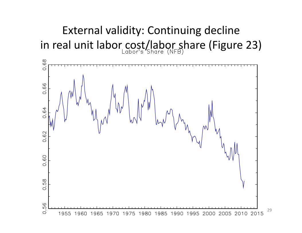
External validity: Continuing decline in real unit labor cost/labor share (Figure 23)

29

Recent Decade: GG model (Figure 24A)

30

Recent decade: SW model (Figure 24B)

31

Comments

• Standard NKPE in GG form is hit by decline in real ulc, as SW form is hit by even more pronounced decline in modified rulc.

• SW had to grapple with this phenomenon earlier, due to early 1990s data revisions (which make our replication of GG look less good than their Figure 2) and longer estimation interval (through 2004:4, which includes some of pronounced recent decline in labor’s share)

32

Another interpretation and its implications

• Labor’s share and labor substitution

• Possibility: roughly constant inflation, roughly constant correctly measured costs, trend down in labor’s share 

33

ateindetermin Shares ]y

wN[

ceindifferenFactor w/x q logs no :Note )(

yqs

sxNay

Summary

• We have studied the link between inflation and unit labor cost, through the NKPE lens

• We have shown how SW model identifies trend declines in modified real unit labor costs as positive price shocks so as to satisfy NKPE

• We have illustrated how labor substitution in the production function could lead to major declines in labor’s share/real unit labor cost without pronounced declines in inflation 

34