INFLATION AND INNOVATION VALUE: HOW INFLATION AFFECTS

Estudios económicos N° 76, Enero - Junio 2020. 147-195 147

INFLATION AND INNOVATION VALUE: HOW INFLATION AFFECTS INNOVATION...ACTORES, CONTRATOS Y MECANISMOS DE PAGO: EL CASO DEL SISTEMA DE SALUD DE NEUQUEN

° Rocha, L. A, Cardenas, L. Q, Alves Reis, F., Araújo Silva, N. G., &, Soares De Almeida, C. A. (2021). Inflation and innovation value: how inflation affects innovation and the value strategy across firms, Estudios económicos, 38(76), pp. 147-195.

* Universidade Federal Rural do Semi-Árido, Brazil. E-mail: [email protected]. ORCID: https://orcid.org/0000-0003-2777-0702.

** Universidade Federal Rural do Semi-Árido, Brazil. E-mail: [email protected]. ORCID: https://orcid.org/0000-0002-7966-3311.

*** Universidade Federal Rural de Pernabuco, Brazil. E-mail: [email protected]. ORCID: https://orcid.org/0000-0003-3578-5357.

¤ Universidade Federal Rural do Semi-Árido, Brazil. E-mail: [email protected]. ORCID: https://orcid.org/0000-0002-3342-5975.

¤¤ Universidade Federal Rural do Semi-Árido, Brazil. Email: [email protected]. ORCID: https://orcid.org/0000-0002-8350-2094.

Estudios económicos. Vol. XXXVIII (N.S.), N° 76, Enero- Junio 2021. 147-195

ISSN 0425-368X (versión impresa) / ISSN (versión digital) 2525-1295

INFLATION AND INNOVATION VALUE: HOW INFLATION AFFECTS INNOVATION AND THE

VALUE STRATEGY ACROSS FIRMS°

INFLAÇÃO E O VALOR DA INOVAÇÃO: COMO A INFLAÇÃO AFETA A INOVAÇÃO E A ESTRATÉGIA DE VALOR DAS FIRMAS

Leonardo Andrade Rocha*

Leonardo Querido Cardenas**

Felipe Alves Reis***

Napie Galve Araújo Silva¤

Carlos Alano Soares De Almeida¤¤

enviado: 9 junio 2020 – aceptado: 22 octubre 2020

Abstract

This research analyzes the effects of inflation on R&D investments and innovation--driven growth. For this, an innovation-driven growth model was built in which firms invest own resources and resources from financial institutions. Credit costs depend on the interest rate charged by these institutions. In an inflation-targeting regime, the monetary authority adjusts the nominal interest rate in order to converge current inflation to the established target. It adjusts the interest rate of financial ins-titutions, changing the opportunity cost of investments. As a result, rising inflation

Estudios económicos N° 76, Enero - Junio 2020. 147-195148

ESTUDIOS ECONOMICOS

promotes a reduction in R&D investments demand, reducing the rate of technolo-gical progress. In the empirical exercise of the model, the estimated coefficient of elasticity of R&D investments is negatively affected by inflation.

Keywords: Innovation, inflation, R&D.JEL Codes: E41, O41.

Resumo

O presente estudo analisa os efeitos da inflação nos investimentos em P&D e no crescimento orientado pela inovação. Para isto, foi construído um modelo de cresci-mento orientado pela inovação de forma que as firmas investem recursos próprios e captam outros recursos junto às instituições financeiras. Os custos dos empréstimos dependem da taxa de juros cobrada pelas instituições financeiras. Em um regime de metas, a autoridade monetária ajusta a taxa de juros nominal no intuito de fazer convergir a inflação corrente para a meta estabelecida. Este processo ajusta a taxa de juros cobrada pelas instituições financeiras elevando o custo de oportunidade dos investimentos. Como resultado, o aumento da inflação promove uma redução na demanda por investimentos em P&D, reduzindo a taxa de progresso tecnológico. No exercício empírico do modelo, o coeficiente estimado de elasticidade dos in-vestimentos em P&D é negativamente afetado pela inflação.

Palabras chaves: inovação, inflação, I&D.Classificação JEL: E41, O41.


INFLATION AND INNOVATION VALUE: HOW INFLATION AFFECTS INNOVATION...

I. INTRODUCTION

Economic theory has always pointed to the harmful effects of inflation on the growth of economies, whether through expectations, the costs of investing, the difficulty of predicting relative prices in the future or even the political aspects associated with austerity measures of macroeconomic policy (Dressler, 2016). In general, it is understood that macroeconomic policy is clearly important for eco-nomic growth because of its role in reducing uncertainty and encouraging invest-ment by economic agents (Barro & Sala-I-Martin, 2004; Aghion & Howitt, 2009; Acemoglu, 2009; Ramzi & Viem, 2016).

While this broad relationship has long been debated over the years, few studies have analyzed the transmission channels which inflation exerts on specific investments, including those that are fundamental to national economic progress: investments in research and development (R&D). Since the contributions of Solow (1956) on how technological advances are critical to the accumulation of wealth in economies, many important studies sought to demonstrate the role of technology and its development in the differences in growth between the various economies (Hall & Jones, 1999; Aghion & Howitt, 2009; Acemoglu, 2009).

Although the debate about inflation costs related to growth has been the subject of several studies in the last 50-60 years (Blanchard, 2016; Brunnermeier & Sannikov, 2016), few studies have examined the impact on specific investments in R&D and, hence, in innovation. Such investments, as Aghion and Howitt (2009), Hall (2002), Hall, Lotti, and Mairesse (2013), Hall, Mairesse, and Mohnen (2010), and Aghion, Howitt, and Prantl (2015), represent one of the basic inputs for innovation and techno-logical progress, since it aligns the creation of a new technology, whether in products, processes, or forms of management, with the firms’ value strategy (Coad, 2011).

In this perspective, these features have very particular characteristics, since they represent over 50% of the wages for a highly qualified workforce. In this case, human resources become a valuable asset of the firms and are subject to agreements of unique characteristics (Hall, 2002). In this way, the predictability of assets and the formation of prices are crucial in the decision making on investments in R&D, as such prices reflect a possible anticipation of the future growth of firms (Kung & Schmid, 2015). In addition, recent empirical evidence shows that investments in R&D are strongly affected by the cash requirements of enterprises.

Considering these aspects, the following questions arise: how does inflation affect the ‘innovation x market value’ of firms? Can inflation represent an advantage


ESTUDIOS ECONOMICOS

for the firms’ value strategy? In order to answer these questions, this study developed a Schumpeterian growth model, relating the efforts in innovation with the resource constraints of firms. The biggest advantage of this theoretical approach is to study the firms’ behavior in conditions of competition, where the prize for innovation is the temporary monopoly associated with the creation of technology (Aghion, Akcigit, & Howitt, 2013). As highlights of the theoretical model, we can list:

1. Firms have financial resources constraints, so that part of the investments are funded by financial institutions through loans;

2. Credit costs are assigned by the interest rate charged by banks that depend on the spread established plus the interest rate set by the monetary authority in order to converge the current inflation to the target set (targeting regime);

3. Unlike Chu and Lai (2013) and Chu et al. (2015), the inclusion of targets in the model has to be a more realistic way to measure the effect of inflation by adjus-ting the interest rate, given the popularity of the targeting regime (Wash, 2003; Ozdemir & Tuzunturk, 2009; Umar, Dahalan, & Aziz, 2016; Hosny, 2017). In this case, the target system becomes important in three factors: (1) in addition to controlling inflation, it reduces its volatility over time; (2) it minimizes the real costs of disinflation; (3) it approaches the long-term inflation expectations established by the target (Capistran & Ramos-France, 2010).

The model results indicate a negative effect between inflation on the demand for R&D and, hence, the rate of technological progress. In the empirical exercise model, the results reveal that inflation reduces the elasticity coefficient of R&D in the market value of firms. Moreover, a non-linear relation is identified between inflation and the value of firms; low and moderate levels have a positive relationship with the value, while high levels imply reduction. The study’s findings indicate that modest inflation may have a positive alignment with the firms’ value strategy, but with a negative result on the investment in applied R&D (elasticity coefficient).

II. THEORETICAL MODEL

Many models disregard the influences of the financial market and financial intermediation (banks) in the growth process and how this process is related to efforts in innovation by businesses. This is because firms always seek to finance part of the total investments allocated to R&D activities (Acemoglu, 2009).

An important and recent contribution in this regard is found in Chu et al. (2020), who dealt with the role of credit restrictions in stimulating or not stimula-



ting innovation, according to different patent protection regimes. Thus, in markets with credit restrictions, strengthening patent protection implies limiting/stifling local R&D demand, compromising innovation.

However, each economy has a relatively distinct economic environment, especially because different types of monetary policies are applied to ensure price stability. The traditional monetary policy implemented in several countries is orien-ted towards controlling the economy’s basic interest rate. In this way, the central bank influences the loan rates that are offered by banks, both non-financial institu-tions and individuals, conditioning, hence, the dynamics of inflation and economic growth (Becker, Orborn, & Yildirim, 2012).

II.2. A Schumpeterian Economy

Growth models based on Schumpeterian assumptions have attracted the atten-tion of many researchers since they have highlighted the key role of innovation for economic growth. This growth is due to the development of innovations that lead to the “destruction” of current technologies, making them obsolete, and replacing them with a new generation of techniques and products (Aghion & Howitt, 2009).

The model is based on a discrete sequence of time periods . In each period there is a stock of labor consisting of L individuals who work aimed at maximizing the expected consumption and that, in this study, will be normalized to a unit (L = 1). This normalization follows the approach presented by Aghion and Howitt (2009), as a way of reducing the model, without many losses of generality, when considering that individuals, each of whom, live only for that period t. Thus, we restrict the effects of population growth to the model.

The economy has a fixed population L, which we normalize to unity. Everyone is endowed with one unit of labor services in the first period and none in the second, and is risk neutral. (Aghion & Howitt, 2009, p. 130).

The final product is created using a flux “i” of intermediate inputs ( ) continuous under the condition , according to the production function:

(1)

The productivity parameter reflects the quality of the intermediate input of sector “i” in the time “t”. Although production of the final good will occur in a competitive


ESTUDIOS ECONOMICOS

market, the intermediate inputs sector is monopolized by the leading firm in the current technology. In this case, the monopolist enjoys profits in the short term, as they create the new current generation of inputs with the best quality. The demand curve for the monopolist is given by the partial derivative:

(2)

The monopolist seeks to maximize the profit function of the sector( ), replacing the demand curve in function:

(3)

The monopolist’s equilibrium profits are obtained by replacing (3) on the profit function, giving the equilibrium level:

(4)

II.3. R&D and Technical Progress

Advances in productivity occur as improvements in future generations of inputs, so that each new generation implies a significant advance in the current quality:

(5)

In certain situations, the innovation carried out does not achieve the expec-ted result and the improvement is not accepted in the market. In this case, producti-vity does not increase and is assumed to remain unchanged, . The size of innovation is given by the parameter, exogenously determined. To increase the chances of a successful innovation, the entrepreneur funds research activity through large investments in R&D, which is represented by the variable . Thus, the greater the effort in innovation through applying considerable resources, the greater the chances of success for the research and, therefore, for the new tech-nology. The function that captures the probability of innovation success is called ‘innovation function’:



(6)

According to Equation (6), the parameters represent, respectively, the research productivity and the elasticity coefficient of R&D. In this sense, the more the productivity can advance technologically in the next period, the greater the probability of success of the research:

(7)

Technological advances observed in the sector are the residual advance of expected productivity, since investments in research are always subject to uncertainty:

(8)

If innovation is successful, profits in the industry are appropriated by the monopolist. However, in the absence of success, the entrepreneur has the sunk costs equivalent to the total investment. Expected profits are adjusted for produc-tivity, reflecting that the entrepreneur seek the highest profits by generated assets

1. Page 153:

Expected profits are adjusted for productivity, reflecting that the entrepreneur

seek the highest profits by generated assets ( = )

Equation (9a): = á

2. Page 154:

Equation (11): = +In (11), represents (…)

3. Page 155:

Equation (12a): = á ( )

4. Page 156:

Equation (15): = + ( ) = ; =

5. Page 157:

Equation (18): = + ( ) = ; =

6. Page 161:

Eq.1( )

= + ( & ) + + [ ( & ) ]+ ( ) + + + + + +

7. Page 179:

Second paragraph: Replace "Figures 2 and 3 illustrates" for "Figures 2 and 3

illustrate"

.

Thus, the entrepreneur allocates the R&D resources to maximize expected profits adjusted for productivity:

1. Page 153:



Equation (9a): = á

2. Page 154:


3. Page 155:


4. Page 156:

Equation (15): = + ( ) = ; =

5. Page 157:

Equation (18): = + ( ) = ; =

6. Page 161:

Eq.1( )

= + ( & ) + + [ ( & ) ]+ ( ) + + + + + +

7. Page 179:


illustrate"

(9a)

(9b)

(9c)

The rate of technological progress is obtained by substituting (9c) to (8):

(10)


ESTUDIOS ECONOMICOS

II.3. Bank-Funded Researches

Only a portion of the investment in research is funded with the monopolist entrepreneur’s own resources. Another part is acquired through loans with banks. Take entrepreneur’s income as . Banks finance only a portion of the investment, forcing the entrepreneur to have financial guarantees. Assuming the monopolist allocates all their income, the financing they get is the difference equivalent to

. Banks, on the other hand, charge interest (r) on the total invest-ment to offset losses generated by funded projects, which subsequently did not have the desired economic viability. The interest rate is based on the following formula:

1. Page 153:



Equation (9a): = á

2. Page 154:


3. Page 155:


4. Page 156:

Equation (15): = + ( ) = ; =

5. Page 157:

Equation (18): = + ( ) = ; =

6. Page 161:

Eq.1( )

= + ( & ) + + [ ( & ) ]+ ( ) + + + + + +

7. Page 179:


illustrate"

(11)

In (11),

1. Page 153:



Equation (9a): = á

2. Page 154:


3. Page 155:


4. Page 156:

Equation (15): = + ( ) = ; =

5. Page 157:

Equation (18): = + ( ) = ; =

6. Page 161:

Eq.1( )

= + ( & ) + + [ ( & ) ]+ ( ) + + + + + +

7. Page 179:


illustrate"

represents the interest rate determined by the monetary autho-rity, and is the additional costs that set the bank interest. The basic interest rate of the economy adjusts the final interest charged by banks on loans, serving as a ‘minimum’ for the definition of money opportunity cost. The high risk involved in financing activities raises an additional cost which, together with the absence of limiting mechanisms in tariff charges, adds the composition of the bank spread1.

Sunk costs of research are now represented by the total volume invested plus interest charged as a result of financing. The sum of the two components defines the total cost of the research: .

In this scenario, we highlight an important limitation of the theoretical model: secondary effects of inflation on important measures of firms. Kang and Pflueger (2015, pp.115-117) found evidence that the effects of inflation can help explain, at least, a direct variation in credit spreads, in addition to volatility in stocks (e.g. Aliyu (2012)) and in the dividend index-price. As Kang and Pflueger (2015) argued:

We find that inflation risk can explain at least as much variation in credit spreads as can equity volatility and the dividend-price ratio. First, more volatile inflation increases the ex ante probability that firms will default due to high real liabilities. Second, when inflation and real cash flows

1 Following Gropp, Sørensen, and Lichtenberger (2007), an important difference between lending rates and market interest rates can be attributed to credit risk, reflecting the likely possibility that some loans may not be fully paid by agents. See Were and Wambua (2014).



are highly correlated, there is a risk of low inflation recessions. In this case, low real cash flows and high real liabilities tend to hit firms at the same time, and this interaction increases default rates and real investor losses. Moreover, inflation cyclicality may also increase the default risk premium in credit spreads if investors are risk averse. (Kang & Pflueger, 2015, pp. 115116).

Such factors contribute, to some extent, to a final effect on the value of firms in the stock market. Other evidence also points to the reflexes on the behavior of companies, which adjust their capital structure in response to the risk of persistent inflation over time (e.g. Hackbarth, Miao, & Morellec, 2006; Chen, Collin-Du-fresne, & Goldstein, 2009; Bhamra, Kuehn, & Strebulaev, 2010; Gomes & Schmid, 2010; Gourio, 2013).

Although this model has been limited in the consequences of inflation in interest rates, an improvement of the model in the future may contribute to greater theoretical robustness.

Reframing (9.a), the new entrepreneur optimization problem incorporates the total cost of the research:

1. Page 153:



Equation (9a): = á

2. Page 154:


3. Page 155:


4. Page 156:

Equation (15): = + ( ) = ; =

5. Page 157:

Equation (18): = + ( ) = ; =

6. Page 161:

Eq.1( )

= + ( & ) + + [ ( & ) ]+ ( ) + + + + + +

7. Page 179:


illustrate"

(12a)

(12b)

(12c)

As in Equations (12b) and (12c), the interest rate acts discounting the effective value of the investment, reflecting a smaller amount of allocated resources in R&D activities and, consequently, in the success of innovation (measured by probability).

Substituting (12c) into (8), the equilibrium technical progress rate is obtained:

(13)


ESTUDIOS ECONOMICOS

(14)

Equation (14) illustrates the influence of interest rates on the rate of tech-nological progress, negatively affecting it. Thus, in economies with higher interest rates, the demand for investment tends to be lower, reducing the necessary efforts to sustain the rate of technological progress.

II.4. Introducing Monetary Policy

The role of the central bank, either in developed or developing economies, is focused on the pursuit of price stability, making the basic interest rate one of the main instruments of monetary policy (Stein, 2012). Several authors argue that the choice of a price index, such as monitoring over time, was gradually guided by the idea that inflation is, in fact, a monetary phenomenon (Goodfriend, 2007; Mishkin, 2007, 2008; Wynne, 2008; Stein, 2012; Anand, Prasad, & Zhang, 2015). As observed by Taylor (2000, p. 90), “monetary-policy decisions are best thought of as rules, or reaction functions, in which the short-term nominal interest rate (the instrument of policy) is adjusted in reaction to economic events.”

This model assumes that the monetary authority acts by controlling the monetary policy in order to converge the current inflation toward the center of the target set. Thus, the deviation caused between current inflation and the center of the target determines the position of the authority to increase or reduce the interest according to the direction of the deviation. This relationship can be expressed as the change in the interest rate (r *):

1. Page 153:



Equation (9a): = á

2. Page 154:


3. Page 155:


4. Page 156:

Equation (15): = + ( ) = ; =

5. Page 157:

Equation (18): = + ( ) = ; =

6. Page 161:

Eq.1( )

= + ( & ) + + [ ( & ) ]+ ( ) + + + + + +

7. Page 179:


illustrate"

(15)

According to Equation (15), inflation ( ) is measured by the percentage change in the general price level, integrating all sectors of the economy. Thus, the monetary authority establishes a target ( ), in order to adjust the interest rate to the extent that the current inflation deviates from the established target. When inflation exceeds the target, the central bank increases the rate of interest in order to ‘level’ economic activity, hence converging inflation to the target set. The para-meters , represent, respectively, the shift term and the elasticity of the inflation deviation.



II.5. Consequences of Inflation Rates Persistently Above Target

In economies where inflation runs persistently above the target set by the monetary authority, it is common to observe high interest rates. As a result, the demand for investments decreases, especially in R&D activities, whose return on investment consists of medium and long term (Hall, Lotti, & Mairesse, 2013).

Modifying Equation (12b) incorporating (15), we have:

(16)

As Equation (16), a persistent rise in inflation above the target prompts the monetary authority to increase interest rates and, consequently, the demand for investments in R&D decreases. With higher interest rates, the cost of capital rises, reducing demand and efforts in innovation. This reduction, in turn, implies a lower probability of success of the innovative entrepreneur, restricting the rate of technical progress in the industry.

(17)

By integrating the sectors of the economy, the rate of technical progress in this economy is reached:

(18)

According to Equation (18), we can observe an inverse relation between inflation and the rate of technological progress in the economy. This relation is not as recent as it may seem, although few studies have focused their analysis on this subject. A pioneering and major study linking the effects of inflation on innovation consists of the contributions of Mansfield (1980). According to the author, as inflation reduces investment rates, it discourages the demand for machinery and equipment, as well as expansion of new plants, limiting the application of specific investments such as R&D. Another important inflation effect consists of public research funding. In developing economies, most of the investments in R&D activities come from public

1. Page 153:



Equation (9a): = á

2. Page 154:


3. Page 155:


4. Page 156:

Equation (15): = + ( ) = ; =

5. Page 157:

Equation (18): = + ( ) = ; =

6. Page 161:

Eq.1( )

= + ( & ) + + [ ( & ) ]+ ( ) + + + + + +

7. Page 179:


illustrate"


ESTUDIOS ECONOMICOS

funds. In these circumstances, governments may be compelled to ‘cut’ a portion of the budget as part of the goal of anti-inflationary fiscal policy.

In this way, research funding may be limited in the implementation of future budgets, restricting the long-term productivity growth. Thus, in order to control rising inflation, economic policy can be directed to promote an ‘undesirable effect’ to reduce the long-term growth2. Such institutional efforts can explain how deve-loping economies with higher inflation rates also have significant limitations for convergence towards the technology frontier. Thus, in the presence of credit cons-traints, through funding research, inflation has a direct impact on the financing interest, raising the opportunity cost of investments in R&D (Chu & Lai, 2013).

III. RESEARCH METHODOLOGY

III.1. Data Source and Sample Delimitation

The data used in this study were extracted from an important data source: Standard and Poor’s (S&P) Capital IQ Platform. The S&P Capital IQ Platform is an important source of financial information, containing financial data from more than 1 million firms worldwide. The main advantage of this platform is the brea-dth of data, separated by countries and sectors, in addition to including the most important financial indicators of companies, which allows a more detailed analysis of the firms’ strategy. The following filters were used:

(i) active firms in the world with legal origin by country and defined market value (publicly traded companies);

(ii) Firms classified according to international credit rating industry classification3; (iii) Firms identified with the digit-1 of the ‘SIC Codes’ corresponding to 10 sectors;(iv) Financial variables from 2010 to 2015 (six years);(v) The final sample was 34 194 firms from 125 countries distributed over the

years 2010 to 2015, corresponding to a panel with 205 164 observations.

2 “Serious inflation can have a significant effect on government financed R&D if it stimulates an anti-inflationary tax policy that affects the size and type of government R&D programs” (Mansfield, 1980, p. 1093).

3 The Standard Industrial Classification (SIC) offers 4-digit industry classification (Sector, majority group, group of industries, and industry). For more details, see: http://siccode.com/en/pages/what-is-a-sic-code



Macroeconomic data were extracted from a relevant international rating company, which calculates risk indicators for 140 countries in the world, Political Risk Services Group. This company measures and analyzes twenty-two variables to define and estimate risk prediction models for international investors divided into three subgroups in the International Country Risk Guide report: twelve political risk variables, five financial risk variables, and five economic risk variables. An impor-tant advantage of the available database consists of a wide time period from 1984 to the present, which allows a better control on the forecast measures and adequacy of variables (Charron, 2011). Given the importance of the quality of risk measures, recent studies have applied the basis of risk analysis at the macroeconomic level (Osabutey & Okoro, 2015; Stockemer, 2013; Kunieda, Okada, & Shibata, 2016; Myles & Yousefi, 2015; Beal & Graham, 2014).

III.2. Operation and Definition of Variables

The variables used in the study are presented in Table 1, with a distinction between variable groups by micro and macro level:

Table 1. Description of the model variables

Variables Definition Applied research

Financial variables (micro-level)

R&D

Investments made in research activities and which may occur internally in firms or externally, through universities and research institutes. Such investments represent the financial effort of the firm in order to finance: new product development on innovative technology formulation, process development, and processes performed in product update or existing service line.

Hall, Mairesse, & Mohnen (2010), Bogliacino & Cordona (2010), Hall, Lotti, & Mairesse (2013), Montresor & Vezzani (2015), and Kancs & Siliverstovs (2016)

mkt_cap Market capitalization value. Dias (2013)

capexInvestments in order to acquire or upgrade physical assets such as equipment, properties, and industrial plants.

Hall (2002), Hall, Lotti, & Mairesse (2008, 2013), Hall, Mairesse & Mohnen (2010), Gupta, Banerjee, & Onur (2017)


ESTUDIOS ECONOMICOS

ATV Total assets. Hall (2002) & Hall, Lotti, and Mairesse (2008, 2013)

Q-Tobin Ratio of market capitalization to total assets.

Coad (2011), Gupta, Onur, & Banerjee (2017), and Hall, Jaffe, & Trajtenberg (2005)

LT_inv Long-term investments represent investments held for more than a year in the firm’s activities.

Graham, Campbell & Rajgopal (2005), Lerner, Sorensen, & Strömberg (2011), and Bourke & Roper (2017)

ST_invShort-term investments represent relatively liquid investments, i.e. activities of the firm of more than three months and less than one year.

Bourke & Roper (2017) and Cremers, Pareek, & Sautner (2017)

Macroeconomic variables

gdp_growth

GDP growth rate, calculated as the percentage change of the current year compared to the previous year.

Bashir (2002), Aghion & Howitt (2009), and Aghion & Jaravel (2015)

gdp_budget

Corresponds to the balance of the central government budget (including grants) for a given year in the national currency and is expressed as a percentage of GDP this year in the national currency.

Aghion & Marinescu (2007), Aghion, Hémous, & Kharroubi (2014)

gdp_current

Corresponds to the balance of payments balance for a given year, converted into US dollars at the average exchange rate for that year. It is expressed as a percentage of GDP, converted into US dollars at the average exchange rate for that year.

Gehringer (2013) and Ege & Ege (2017)

gdp_exp

Corresponds to the balance of payments balance for a given year, converted into US dollars at the average exchange rate for that year. It is expressed as a percentage of total exports of the country’s goods and services, converted into US dollars at the average exchange rate for that year.

Aghion & Marinescu (2007) and Gehringer (2013)



inflInflation rate that is obtained annually through the unweighted average of the Consumer Price Index.

Bashir (2002), Funk & Kromen (2010), Chu & Lai (2013), Ascari & Sbordone (2014) and Anand, Prasad & Zhang (2015)

Source: Prepared by the authors.Note: The column “Applied Research” lists the studies that used the variables cited in research related to the topic discussed.

III.3. Regression Model

To analyze the effects of investments in R&D on firms’ innovation, a portion of the literature on the topic applies traditional sales performance measures to asso-ciate with investments in research. However, we prefer to adopt the value of firms as a performance measure, based on Tobin’s Q indicator. This choice minimizes potential problems related to time lags between the firm’s behavior and changes in performance, since “future performance gains obtained through ‘appropriate’ behavior can be anticipated on the stock market and can thus be included into a firm’s current market value (and hence Tobin’s q)” (COAD, 2011, p. 1054).

Moreover, the market value better reflects the returns of innovation, in addi-tion to allowing a better comparison of the productivity of innovation according to different markets and production technologies, making it difficult to compare the productivity levels of these firms (Hall, Jaffe, & Trajtenberg, 2005; Hall, Mairesse, & Mohnen, 2010).

To study the effect of inflation in relation to “investment x performance”, the following equation was estimated:

Eq. 1

1. Page 153:



Equation (9a): = á

2. Page 154:


3. Page 155:


4. Page 156:

Equation (15): = + ( ) = ; =

5. Page 157:

Equation (18): = + ( ) = ; =

6. Page 161:

Eq.1( )

= + ( & ) + + [ ( & ) ]+ ( ) + + + + + +

7. Page 179:


illustrate"

According to Eq.1, the firm’s value, calculated through the Q-Tobin, is regres-sed with R&D, inflation, cross-effects between inflation and investment and inflation rate squared. The Xmicro vector represents the set of variables at the financial level


ESTUDIOS ECONOMICOS

of firms that help to control important characteristics of the value strategy (capex, assets, and short and long-term investments). The other vector, Xmacro, relates to the macro-level dimensions that condition firms’ strategies and help to control the greater latent effects of inflation on economies. The subscripts i, j, r, and t represent, respectively, the dimensions at the level of firm, sector, economic region, and year.

Additional vectors , , correspond to the fixed effects at the sectoral, regional, and temporal level, affect the firms’ value strategy based on the invest-ments made and control the effects at the macroeconomic level in the ‘investment x performance’ relation. The stochastic error is captured , representing all other factors that are not part of the research scope, being irrelevant to the model.

III.4. Estimation Method and Robustness

Eq.1 can be estimated by the traditional ordinary least squares technique (OLS), grouping the data and disregarding the fixed effects in the main model. However, the absence of fixed effects may lead to a serious bias in estimates that do not disappear even when the sample is relatively large (Greene, 2012). In this case, regional and sectoral factors exert a significant influence, either on the demand for investments or on the macroeconomic scenario, through differences between fiscal and monetary policies, affecting inflation rates. Specific market structures can induce specific investment demands, affecting the relation between regressors and the secto-ral fixed effects (Coad, 2011). Such movements can present a systematic correlation with the stochastic disturbance, leading to an inconsistency in the estimates.

The inclusion of fixed effects controls such latent effects of the stochastic disturbance and the covariates. In this case, the regression technique with traditio-nal panel data includes another important factor in the size of the fixed effects: the individual factor or individual heterogeneity effect. However, the sample is cha-racterized by an important singularity that consists of a panel with a cross-sectional dimension much larger than the temporal section (called short panel).

In a sample with these characteristics, recent research, especially Hahn and Kuersteiner (2002), Hahn and Newey (2004), Lee and Phillips (2015), and Bester and Hansen (2016), have pointed out the relative problems in models with panel data when the cross-section is considerably higher than the temporal cut (short panel) – see Hsiao (2014). This phenomenon, called “incidence of parameters pro-blem”, was firstly diagnosed by Neyman and Scott (1948).



As shown by Hahn and Newey (2004), the parameters of the variables of interest are inconsistent when the number of individuals (n) becomes sufficiently large relative to the time period (T). This inconsistency stems from the finite num-ber of observations that are available to estimate each individual effect (signifi-cantly reducing the degree of freedom of the model).

An alternative form, proposed by Bester and Hansen (2016), consists in esti-mating the fixed effects by aggregating the individual effects at different levels of pre-determined groups. In the same way that the authors in the study, in microdata on teaching evaluation, students can be grouped according to classes, education levels, schools, and districts; or even firms can be grouped according to different sectoral levels or specific economic regions. This technique, called ‘grouped effects estimator’, considers the estimation of model parameters by treating individual specific effects as constant within groups at a particular level.

Therefore, this research implements an adaptation of the model proposed by Bester and Hansen (2016) in non-linear functions for the panel data methodology. In this case, the executed technique excludes the individual effects, aggregating them by regional and sectorial level, executing a procedure of grouped fixed effects. This derives from a large amplitude of the cross-sectional sample that includes 34,194 firms over 6 years. The inclusion of fixed effects at the firm level would entail serious damage to the model, what makes necessary treatment from the tech-nique proposed by Bester and Hansen (2016) adapted to a linear model. Lastly, the parameter covariance matrix was estimated using the residual clustering technique, having the individual units as dimension to correct serial autocorrelation and hete-roscedasticity. Thus, the standard-error estimative are consistent and parameters are efficient (Greene, 2012).

Although, in the model, a more in-depth investigation is not applied on the existence or not of stationarity in the data, the presence of panel data with very large cross-section units (and T-small) make these limitations relatively easier to be addressed. Circumvented, assuming some restrictions, such as homogeneity in the slope coefficients (e.g. Baltagi, 2005, pp. 201) and independence of obser-vations between the cross-sectional units (e.g. Hsiao, 2014, p. 9). Although this assumption is strong, the control of heterogeneity to the model can be sustained in many situations. These advantages are relatively greater in panel models with N-large, which are adherent with the sample of the present study. In addition, the comparison with the dynamic panel technique allowed a better correlation of the results that demonstrated a relative convergence in the understanding. Furthermore, based on the assumption that the observations between the transversal units are


ESTUDIOS ECONOMICOS

independent, especially in samples with N-large and T-small (e.g. Hsiao, 2003, p. 7; 2007, p. 5; 2014, p. 386-387), we can appropriate the Central Limit Theorem between the transversal units to show that the distributions of many estimators remain asymptotically normal (e.g. Binder, Hsiao, & Pesaran, 2005, Im, Pesaran, & Shin, 2003), Levin, Lin, & Chu, 2002). It is also necessary to point out that, in series at the level of microdata, relatively large cross-sectional units with limited time space are common, involving relatively small T values, so it is natural to assume that the series follow stationary processes (see Hall & Urga, 2000, p. 2).

III.5. Dynamic Effects of Firms’ Value

Another way to estimate the Eq.1 model is to include the lagged effect of the dependent variable. In general notation, this implies adjusting the model as:

Eq.2

The parameter to be estimated “ ” captures the persistent effect of the firm’s value over time. The vector of parameters of the independent variables is determined by “ ”. The fixed effects related to the firm level are captured by “ ”, and the temporal effects by “ ”. The error term is defined by “ ”.

One of the great contributions in the econometrics of dynamic models con-sists of the study developed by Arellano and Bond (1991), who proposed the use of the Difference GMM estimator (Generalized Method of Moments). This procedure consists in transforming the data through differences in time and addressing the problem of endogeneity through the use of lagged values as instruments. Subse-quently, this technique demonstrated limited performance, especially in conditions close to the present study: when the time cut is relatively small compared to the cross-section (cross-section, N> T) and when the dependent variable tends to show a persistence pattern in time. Such factors are limiting to the difference GMM technique, being subject to a large sample bias (Arellano & Bover, 1995; Blundell & Bond, 1998; Alonso-Borrego & Arellano, 1999; Arellano, 2016; Jha, 2019).

Based on the contributions of Arellano and Bover (1995) and Blundell and Bond (1998), the System GMM estimator sought to solve such problems: (1) increasing efficiency, since it uses more moment conditions than the difference GMM, which makes it more appropriate for non-stationary data and; (2) ensuring consistency, since it does not depend on the assumption of any second-order serial



correlation (Mehic, 2018). In addition, the combination of factors such as short panel (N> T), lagged dependent variable, inclusion of numerous fixed effects and a lack of good external instruments, make the technique even more attractive in empirical studies (Roodman, 2009).

One of the great advances in the technique is to limit the inclusion of ins-truments to the model, avoiding the “proliferation of instruments”. In this critical problem, the results of the model may suggest a validity, when, in fact, the model is closer to being invalid. This is known in the literature as a false positive, leading to conclusions that are precipitated by the excessive inclusion of non-relevant ins-truments, inflating the model (Roodman, 2009).

The solution to this problem is to “collapse” the instrument matrix, limiting the entry of many outdated instruments. This procedure is duly presented in the contributions of Beck and Levine (2005), Carkovic and Levine (2005) and, later, in Roodman (2009) and Labra and Torrecillas (2018).

IV. RESEARCH RESULTS

IV.1. Descriptive Analysis of the Sample

Table 2 shows the distribution of firms according to the seven geographical regions in the world.

Table 2. Distribution of firms by geographic region

Geographic location Freq. Abs. Freq. Rel. (%) Freq. Cum. (%)

Africa / Middle East 1 645 4.81 4.81

Asia / Pacific 14 494 42.39 47.20

Caribbean 201 0.59 47.79

Central America and Mexico 91 0.27 48.05

Europe 5 976 17.48 65.53

Latin America and Caribbean 448 1.31 66.84

United States and Canada 11 339 33.16 100.00

Total 34 194 100.00 -

Source: prepared by the authors


ESTUDIOS ECONOMICOS

As shown in the table, most of the firms in the sample are in Asia, which represents approximately 42% of the total. Countries from North America (United States of America and Canada) represent approximately 33% and Europe 17.5%. Latin America and the Caribbean correspond to 448 firms, representing about 1.31% of the sample. Africa and the Middle East amount to 1 645 firms (4.81% of the sample).

The distribution of firms by sector, as SIC Codes classification, is shown in the results of Table 3.

Table 3. Distribution of firms by sector

Sector Freq. Abs. Freq. Rel. (%) Freq. Cum. (%)

Division A: Agriculture, Forestry, and Fishing 205 0.60 0.60

Division B: Mining 3 171 9.27 9.87

Division C: Construction 679 1.99 11.86

Division D: Manufacturing 12 709 37.17 49.03

Division E: Transportation, Communications, Electric, Gas, and Sanitary Services

2 133 6.24 55.26

Division F: Wholesale Trade 1 083 3.17 58.43

Division G: Retail Trade 1 174 3.43 61.86

Division H: Finance, Insurance, and Real Estate 8 486 24.82 86.68

Division I: Services 4 177 12.22 98.90

Division J: Public Administration 377 1.10 100.00

Total 34 194 100.00 -

Source: Authors’ calculations.



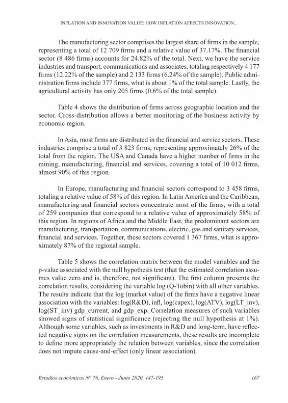
The manufacturing sector comprises the largest share of firms in the sample, representing a total of 12 709 firms and a relative value of 37.17%. The financial sector (8 486 firms) accounts for 24.82% of the total. Next, we have the service industries and transport, communications and associates, totaling respectively 4 177 firms (12.22% of the sample) and 2 133 firms (6.24% of the sample). Public admi-nistration firms include 377 firms, what is about 1% of the total sample. Lastly, the agricultural activity has only 205 firms (0.6% of the total sample).

Table 4 shows the distribution of firms across geographic location and the sector. Cross-distribution allows a better monitoring of the business activity by economic region.

In Asia, most firms are distributed in the financial and service sectors. These industries comprise a total of 3 823 firms, representing approximately 26% of the total from the region. The USA and Canada have a higher number of firms in the mining, manufacturing, financial and services, covering a total of 10 012 firms, almost 90% of this region.

In Europe, manufacturing and financial sectors correspond to 3 458 firms, totaling a relative value of 58% of this region. In Latin America and the Caribbean, manufacturing and financial sectors concentrate most of the firms, with a total of 259 companies that correspond to a relative value of approximately 58% of this region. In regions of Africa and the Middle East, the predominant sectors are manufacturing, transportation, communications, electric, gas and sanitary services, financial and services. Together, these sectors covered 1 367 firms, what is appro-ximately 87% of the regional sample.

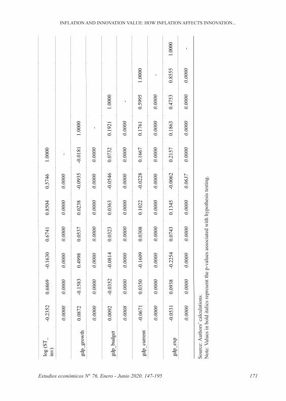
Table 5 shows the correlation matrix between the model variables and the p-value associated with the null hypothesis test (that the estimated correlation assu-mes value zero and is, therefore, not significant). The first column presents the correlation results, considering the variable log (Q-Tobin) with all other variables. The results indicate that the log (market value) of the firms have a negative linear association with the variables: log(R&D), infl, log(capex), log(ATV), log(LT_inv), log(ST_inv) gdp_current, and gdp_exp. Correlation measures of such variables showed signs of statistical significance (rejecting the null hypothesis at 1%). Although some variables, such as investments in R&D and long-term, have reflec-ted negative signs on the correlation measurements, these results are incomplete to define more appropriately the relation between variables, since the correlation does not impute cause-and-effect (only linear association).


ESTUDIOS ECONOMICOS

Tabl

e 4.

Cro

ss-d

istri

butio

n of

firm

s by

geog

raph

ic lo

catio

n an

d in

dust

ry

Sect

or -

SIC

cod

es

Geo

grap

hic

loca

tion

Afr

ica

/ M

iddl

e Ea

st

Asi

a /

Paci

ficC

arib

bean

Cen

tral

Am

eric

a an

d M

exic

o

Euro

pe

Latin

A

mer

ica

and

Car

ibbe

an

Uni

ted

Stat

es a

nd

Can

ada

Tota

l

Div

isio

n A

: Agr

icul

ture

, For

estry

, an

d Fi

shin

g10

122

10

327

3320

5

Div

isio

n B

: Min

ing

7490

131

635

726

1 77

63

171

Div

isio

n C

: Con

stru

ctio

n35

408

03

148

1075

679

Div

isio

n D

: Man

ufac

turin

g53

571

332

262

034

146

2 80

612

709

Div

isio

n E:

Tra

nspo

rtatio

n,

Com

mun

icat

ions

, Ele

ctric

, Gas

, an

d Sa

nita

ry S

ervi

ces

117

853

3619

520

8350

52

133

Div

isio

n F:

Who

lesa

le T

rade

5961

03

017

08

233

1 08

3

Div

isio

n G

: Ret

ail T

rade

5850

25

823

522

344

1 17

4

Div

isio

n H

: Fin

ance

, Ins

uran

ce,

and

Rea

l Est

ate

579

2 20

870

251

424

113

4 06

78

486

Div

isio

n I:

Serv

ices

136

1 61

517

210

224

1 36

34

177

Div

isio

n J:

Pub

lic A

dmin

istra

tion

4214

56

236

913

737

7

Tota

l1

645

14 4

9420

191

5 97

644

811

339

34 1

94

Sour

ce: A

utho

rs’ c

alcu

latio

ns



Tabl

e 4.

Cro

ss-d

istri

butio

n of

firm

s by

geog

raph

ic lo

catio

n an

d in

dust

ry

Sect

or -

SIC

cod

es

Geo

grap

hic

loca

tion

Afr

ica

/ M

iddl

e Ea

st

Asi

a /

Paci

ficC

arib

bean

Cen

tral

Am

eric

a an

d M

exic

o

Euro

pe

Latin

A

mer

ica

and

Car

ibbe

an

Uni

ted

Stat

es a

nd

Can

ada

Tota

l

Div

isio

n A

: Agr

icul

ture

, For

estry

, an

d Fi

shin

g10

122

10

327

3320

5

Div

isio

n B

: Min

ing

7490

131

635

726

1 77

63

171

Div

isio

n C

: Con

stru

ctio

n35

408

03

148

1075

679

Div

isio

n D

: Man

ufac

turin

g53

571

332

262

034

146

2 80

612

709

Div

isio

n E:

Tra

nspo

rtatio

n,

Com

mun

icat

ions

, Ele

ctric

, Gas

, an

d Sa

nita

ry S

ervi

ces

117

853

3619

520

8350

52

133

Div

isio

n F:

Who

lesa

le T

rade

5961

03

017

08

233

1 08

3

Div

isio

n G

: Ret

ail T

rade

5850

25

823

522

344

1 17

4

Div

isio

n H

: Fin

ance

, Ins

uran

ce,

and

Rea

l Est

ate

579

2 20

870

251

424

113

4 06

78

486

Div

isio

n I:

Serv

ices

136

1 61

517

210

224

1 36

34

177

Div

isio

n J:

Pub

lic A

dmin

istra

tion

4214

56

236

913

737

7

Tota

l1

645

14 4

9420

191

5 97

644

811

339

34 1

94

Sour

ce: A

utho

rs’ c

alcu

latio

ns

Investments in research showed an inverse linear association, in addition to the log (Q-Tobin), with inflation, the growth rate, and the balance of public budget/GDP. The calculated measures presented statistical significance at 1%. It is necessary to note that the extent of correlation between log (Q-Tobin) and inflation showed a low magnitude. However, log(R&D) and inflation presented a much higher magnitude, equivalent to four times compared to the previous one. It deno-tes a greater sensitivity of association of the investment in relation to the market value of firms. Table 5 shows the correlation matrix between the model variables and their respective p-values.

IV.2. Results of the Econometric Model

Table 6 presents the results of model ME.1, excluding the quadratic varia-ble of inflation. The isolated effect of investments in R&D was positive in most columns, except for column (2). The isolated elasticity showed results between 0.05% and 0.18% - significant at 1%. With the inclusion of financial variables, the coefficients demonstrated a closer and more stable values with little variation (between 0.114% and 0.12%). Between the columns (2) to (6), inclusion and exclu-sion of financial variables presented higher reflections in the range of possibilities of the coefficients, demonstrating a sensitivity to the micro-dimension variables of firms.

Except for columns (2) and (6), inflation had a positive effect on the market value of firms (significant parameters to 1%, except in columns (5) and (6)). The inclusion/exclusion of micro-dimension variables showed an effect of underestima-ting the impact of inflation, signaling for estimates below the parameter obtained in the complete model (column (1)). In the opposite direction, the inclusion/exclu-sion of variables of macro dimension demonstrated an effect of overestimating the impact of inflation in comparison with the complete model.

Regarding the cross-effect between inflation and investments in R&D, the complete model showed a parameter with a negative and significant sign at 1%. Columns (2), (3), and (6) had a positive effect, however not significant in column (3). The other columns demonstrated negative parameters, but not significant for columns (4) and (5). These results indicate a volatility in the parameters, as we include/exclude the micro-dimension variables, thus revealing a sensitivity with such variables. With the inclusion/exclusion of macro-dimension variables, the coefficient obtained revealed signs of underestimation in relation to the complete model (values in module in columns (8), (9), and (10)).


ESTUDIOS ECONOMICOS

Tabl

e 5.

cor

rela

tion

mat

rix b

etw

een

the

mod

el v

aria

bles

and

thei

r res

pect

ive

p-va

lues

log

(Q-T

obin

)lo

g (R

&D

)infl

log

(cap

ex)

log

(ATV

)lo

g (L

T_in

v)lo

g (S

T_in

v)gd

p_gr

owth

gdp_

budg

etgd

p_cu

rren

tgd

p_ex

p

log

(Q-T

obin

)1.

0000

-

log

(R&

D)

-0.0

343

1.00

00

0.00

00 -

infl

-0.0

745

-0.3

123

1.00

00

0.00

000.

0000

-

log

(cap

ex)

-0.1

360

0.55

030.

0019

1.00

00

0.00

000.

0000

0.50

05 -

log

(ATV

)-0

.433

40.

6423

-0.01

070.

7910

1.00

00

0.00

000.

0000

0.00

000.

0000

-

log

(LT_

inv)

-0.2

669

0.49

12-0

.0945

0.45

670.

7297

1.00

00

0.00

000.

0000

0.00

000.

0000

0.00

00 -

log

(ST_

inv)

-0.2

352

0.68

69-0

.163

00.

6741

0.85

040.

5746

1.00

00

0.00

000.

0000

0.00

000.

0000

0.00

000.

0000

-

gdp_

grow

th0.

0872

-0.1

583

0.49

980.

0537

0.02

38-0

.093

5-0

.018

11.

0000

0.00

000.

0000

0.00

000.

0000

0.00

000.

0000

0.00

00 -

gdp_

budg

et0.

0092

-0.0

352

-0.0

814

0.03

230.

0363

-0.0

546

0.07

320.

1921

1.00

00

0.00

080.

0000

0.00

000.

0000

0.00

000.

0000

0.00

000.

0000

-

gdp_

curr

ent

-0.0

671

0.03

50-0

.160

90.

0308

0.10

22-0

.022

80.

1667

0.17

610.

5995

1.00

00

0.00

000.

0000

0.00

000.

0000

0.00

000.

0000

0.00

000.

0000

0.00

00 -

gdp_

exp

-0.0

531

0.09

38-0

.225

40.

0743

0.13

45-0

.006

20.

2157

0.18

630.

4753

0.85

551.

0000

0.00

000.

0000

0.00

000.

0000

0.00

000.

0637

0.00

000.

0000

0.00

000.

0000

-

Sour

ce: A

utho

rs’ c

alcu

latio

ns.

Not

e: V

alue

s in

bold

ital

ics r

epre

sent

the

p-va

lues

ass

ocia

ted

with

hyp

othe

sis t

estin

g.



Tabl

e 5.

cor

rela

tion

mat

rix b

etw

een

the

mod

el v

aria

bles

and

thei

r res

pect

ive

p-va

lues

log

(Q-T

obin

)lo

g (R

&D

)infl

log

(cap

ex)

log

(ATV

)lo

g (L

T_in

v)lo

g (S

T_in

v)gd

p_gr

owth

gdp_

budg

etgd

p_cu

rren

tgd

p_ex

p

log

(Q-T

obin

)1.

0000

-

log

(R&

D)

-0.0

343

1.00

00

0.00

00 -

infl

-0.0

745

-0.3

123

1.00

00

0.00

000.

0000

-

log

(cap

ex)

-0.1

360

0.55

030.

0019

1.00

00

0.00

000.

0000

0.50

05 -

log

(ATV

)-0

.433

40.

6423

-0.01

070.

7910

1.00

00

0.00

000.

0000

0.00

000.

0000

-

log

(LT_

inv)

-0.2

669

0.49

12-0

.0945

0.45

670.

7297

1.00

00

0.00

000.

0000

0.00

000.

0000

0.00

00 -

log

(ST_

inv)

-0.2

352

0.68

69-0

.163

00.

6741

0.85

040.

5746

1.00

00

0.00

000.

0000

0.00

000.

0000

0.00

000.

0000

-

gdp_

grow

th0.

0872

-0.1

583

0.49

980.

0537

0.02

38-0

.093

5-0

.018

11.

0000

0.00

000.

0000

0.00

000.

0000

0.00

000.

0000

0.00

00 -

gdp_

budg

et0.

0092

-0.0

352

-0.0

814

0.03

230.

0363

-0.0

546

0.07

320.

1921

1.00

00

0.00

080.

0000

0.00

000.

0000

0.00

000.

0000

0.00

000.

0000

-

gdp_

curr

ent

-0.0

671

0.03

50-0

.160

90.

0308

0.10

22-0

.022

80.

1667

0.17

610.

5995

1.00

00

0.00

000.

0000

0.00

000.

0000

0.00

000.

0000

0.00

000.

0000

0.00

00 -

gdp_

exp

-0.0

531

0.09

38-0

.225

40.

0743

0.13

45-0

.006

20.

2157

0.18

630.

4753

0.85

551.

0000

0.00

000.

0000

0.00

000.

0000

0.00

000.

0637

0.00

000.

0000

0.00

000.

0000

-

Sour

ce: A

utho

rs’ c

alcu

latio

ns.

Not

e: V

alue

s in

bold

ital

ics r

epre

sent

the

p-va

lues

ass

ocia

ted

with

hyp

othe

sis t

estin

g.


ESTUDIOS ECONOMICOS

Tabl

e 6.

Mod

el re

sults

. Dep

ende

nt v

aria

ble:

log

(Q-T

obin

)

Var.

inde

pend

ent

(1)

(2)

(3)

(4)

(5)

(6)

(7)

(8)

(9)

(10)

log

(R&

D)

0.11

8***

-0.0

574*

**0.

0947

***

0.18

8***

0.06

28**

*0.

0540

***

0.12

0***

0.11

7***

0.11

4***

0.11

6***

(0.0

0812

)(0

.006

35)

(0.0

0688

)(0

.007

04)

(0.0

0726

)(0

.007

32)

(0.0

0806

)(0

.008

47)

(0.0

0849

)(0

.008

49)

infl

0.04

38**

*-0

.027

4***

0.02

67**

*0.

0298

***

0.00

614

-0.0

103

0.06

02**

*0.

0890

***

0.06

34**

*0.

0804

***

(0.0

0850

)(0

.007

51)

(0.0

0783

)(0

.007

11)

(0.0

0860

)(0

.007

65)

(0.0

0789

)(0

.008

65)

(0.0

0885

)(0

.009

37)

log

(R&

D) *

infl

-0.00

815*

**0.

0113

***

0.00

105

-0.0

0125

-0.0

0011

40.

0076

8***

-0.00

845*

**-0

.005

99**

-0.0

0492

**-0

.005

25**

(0.0

0219

)(0

.001

83)

(0.0

0201

)(0

.001

81)

(0.0

0217

)(0

.001

88)

(0.0

0219

)(0

.002

43)

(0.0

0241

)(0

.002

43)

Var.

finan

cial

(m

icro

-leve

l) -

- - -

- - -

- -

- -- -

- - -

- -

- - -

- -

- -

- - -

- - -

- - -

- -

- - -

- - -

- - -

- -

- -

- - -

- - -

- - -

- - -

- -

- - -

- - -

- -

- - -

- - -

log

(cap

ex)

0.08

68**

*

-0.1

43**

*

0.08

83**

*0.

0983

***

0.09

90**

*0.

100*

**

(0.0

0786

)

(0.0

0420

)

(0.0

0791

)(0

.008

15)

(0.0

0808

)(0

.008

13)

log

(ATV

)-0

.498

***

-0.2

99**

*

-0

.494

***

-0.5

00**

*-0

.508

***

-0.5

04**

*

(0.0

159)

(0.0

0660

)

(0

.016

0)(0

.016

4)(0

.016

3)(0

.016

4)

log

(LT_

inv)

0.01

16**

-0

.064

1***

0.

0114

**0.

0085

2*0.

0092

4*0.

0088

7*

(0.0

0487

)

(0.0

0438

)

(0.0

0488

)(0

.005

08)

(0.0

0503

)(0

.005

05)

log

(ST_

inv)

0.23

7***

-0.1

34**

*0.

234*

**0.

238*

**0.

241*

**0.

239*

**

(0.0

109)

(0.0

0702

)(0

.010

9)(0

.011

1)(0

.011

0)(0

.011

1)

Var.

mac

roec

onom

ic

(mac

ro-le

vel)

- - -

- - -

- -

- - --

- - -

- -

- - -

- - -

- - -

- - -

- -

- - -

- - -

- - -

- - -

- -

- - -

- - -

- - -

- - -

- -

- - -

- - -

- - -

- - -

-

gdp_

grow

th0.

0884

***

0.09

13**

*0.

100*

**0.

0975

***

0.08

20**

*0.

0959

***

0.10

3***

(0.0

0573

)(0

.005

67)

(0.0

0552

)(0

.005

12)

(0.0

0588

)(0

.005

55)

(0.0

0529

)

gdp_

budg

et0.

0072

5**

0.01

45**

*0.

0090

9***

0.00

776*

*0.

0088

2**

0.01

15**

*

0.00

848*

**

(0.0

0362

)(0

.003

60)

(0.0

0335

)(0

.003

09)

(0.0

0370

)(0

.003

46)

(0

.003

21)

gdp_

curr

ent

-0.0

334*

**-0

.030

7***

-0.0

353*

**-0

.034

7***

-0.0

320*

**-0

.032

3***

-0.0

264*

**

(0.0

0423

)(0

.004

01)

(0.0

0380

)(0

.003

64)

(0.0

0450

)(0

.003

87)

(0.0

0302

)

gdp_

exp

0.00

635*

**0.

0006

840.

0074

8***

0.00

720*

**0.

0085

7***

0.00

416*

*

-0.0

0430

**

(0.0

0229

)(0

.002

16)

(0.0

0200

)(0

.001

85)

(0.0

0238

)(0

.002

08)

(0

.001

77)

Con

stan

t1.

248*

**-0

.371

***

-0.1

661.

200*

**-0

.445

***

-0.0

0113

1.09

6***

1.48

9***

1.56

9***

1.50

4***

(0.1

21)

(0.1

16)

(0.1

22)

(0.1

26)

(0.1

16)

(0.1

21)

(0.1

15)

(0.1

21)

(0.1

25)

(0.1

25)

R2

0.33

20.

185

0.23

60.

359

0.24

10.

221

0.32

30.

296

0.30

60.

296

R2 A

dj0.

331

0.18

40.

236

0.35

90.

240

0.22

10.

323

0.29

50.

305

0.29

6

Sam

ple

205

164

205

164

205

164

205

164

205

164

205

164

205

164

205

164

205

164

205

164

F te

st12

7.2*

**15

5.8*

**15

1.5*

**22

2.7*

**12

4.0*

**15

6.9*

**13

3.4*

**12

1.6*

**12

5.0*

**12

2.4*

**

Fixe

d Ef

fect

s (s

ecto

r, re

gion

, and

ye

ar)

Yes

Yes

Yes

Yes

Yes

Yes

Yes

Yes

Yes

Yes

F Fi

xed

Effe

cts T

est

53.7

9***

98.6

9***

53.9

2***

60.1

2***

65.7

1***

76.9

2***

74.2

0***

71.1

6***

75.2

9***

73.8

4***

Sour

ce: A

utho

rs’ c

alcu

latio

ns.

Lege

nd: *

** p

<0.

01, *

* p

<0.0

5, *

p <

0.1.

The

par

amet

ers o

f the

stan

dard

err

or e

stim

ates

are

robu

st fo

r the

pre

senc

e of

het

eros

ceda

stic

ity a

nd

auto

corr

elat

ion.



Tabl

e 6.

Mod

el re

sults

. Dep

ende

nt v

aria

ble:

log

(Q-T

obin

)

Var.

inde

pend

ent

(1)

(2)

(3)

(4)

(5)

(6)

(7)

(8)

(9)

(10)

log

(R&

D)

0.11

8***

-0.0

574*

**0.

0947

***

0.18

8***

0.06

28**

*0.

0540

***

0.12

0***

0.11

7***

0.11

4***

0.11

6***

(0.0

0812

)(0

.006

35)

(0.0

0688

)(0

.007

04)

(0.0

0726

)(0

.007

32)

(0.0

0806

)(0

.008

47)

(0.0

0849

)(0

.008

49)

infl

0.04

38**

*-0

.027

4***

0.02

67**

*0.

0298

***

0.00

614

-0.0

103

0.06

02**

*0.

0890

***

0.06

34**

*0.

0804

***

(0.0

0850

)(0

.007

51)

(0.0

0783

)(0

.007

11)

(0.0

0860

)(0

.007

65)

(0.0

0789

)(0

.008

65)

(0.0

0885

)(0

.009

37)

log

(R&

D) *

infl

-0.00

815*

**0.

0113

***

0.00

105

-0.0

0125

-0.0

0011

40.

0076

8***

-0.00

845*

**-0

.005

99**

-0.0

0492

**-0

.005

25**

(0.0

0219

)(0

.001

83)

(0.0

0201

)(0

.001

81)

(0.0

0217

)(0

.001

88)

(0.0

0219

)(0

.002

43)

(0.0

0241

)(0

.002

43)

Var.

finan

cial

(m

icro

-leve

l) -

- - -

- - -

- -

- -- -

- - -

- -

- - -

- -

- -

- - -

- - -

- - -

- -

- - -

- - -

- - -

- -

- -

- - -

- - -

- - -

- - -

- -

- - -

- - -

- -

- - -

- - -

log

(cap

ex)

0.08

68**

*

-0.1

43**

*

0.08

83**

*0.

0983

***

0.09

90**

*0.

100*

**

(0.0

0786

)

(0.0

0420

)

(0.0

0791

)(0

.008

15)

(0.0

0808

)(0

.008

13)

log

(ATV

)-0

.498

***

-0.2

99**

*

-0

.494

***

-0.5

00**

*-0

.508

***

-0.5

04**

*

(0.0

159)

(0.0

0660

)

(0

.016

0)(0

.016

4)(0

.016

3)(0

.016

4)

log

(LT_

inv)

0.01

16**

-0

.064

1***

0.

0114

**0.

0085

2*0.

0092

4*0.

0088

7*

(0.0

0487

)

(0.0

0438

)

(0.0

0488

)(0

.005

08)

(0.0

0503

)(0

.005

05)

log

(ST_

inv)

0.23

7***

-0.1

34**

*0.

234*

**0.

238*

**0.

241*

**0.

239*

**

(0.0

109)

(0.0

0702

)(0

.010

9)(0

.011

1)(0

.011

0)(0

.011

1)

Var.

mac

roec

onom

ic

(mac

ro-le

vel)

- - -

- - -

- -

- - --

- - -

- -

- - -

- - -

- - -

- - -

- -

- - -

- - -

- - -

- - -

- -

- - -

- - -

- - -

- - -

- -

- - -

- - -

- - -

- - -

-

gdp_

grow

th0.

0884

***

0.09

13**

*0.

100*

**0.

0975

***

0.08

20**

*0.

0959

***

0.10

3***

(0.0

0573

)(0

.005

67)

(0.0

0552

)(0

.005

12)

(0.0

0588

)(0

.005

55)

(0.0

0529

)

gdp_

budg

et0.

0072

5**

0.01

45**

*0.

0090

9***

0.00

776*

*0.

0088

2**

0.01

15**

*

0.00

848*

**

(0.0

0362

)(0

.003

60)

(0.0

0335

)(0

.003

09)

(0.0

0370

)(0

.003

46)

(0

.003

21)

gdp_

curr

ent

-0.0

334*

**-0

.030

7***

-0.0

353*

**-0

.034

7***

-0.0

320*

**-0

.032

3***

-0.0

264*

**

(0.0

0423

)(0

.004

01)

(0.0

0380

)(0

.003

64)

(0.0

0450

)(0

.003

87)

(0.0

0302

)

gdp_

exp

0.00

635*

**0.

0006

840.

0074

8***

0.00

720*

**0.

0085

7***

0.00

416*

*

-0.0

0430

**

(0.0

0229

)(0

.002

16)

(0.0

0200

)(0

.001

85)

(0.0

0238

)(0

.002

08)

(0

.001

77)

Con

stan

t1.

248*

**-0

.371

***

-0.1

661.

200*

**-0

.445

***

-0.0

0113

1.09

6***

1.48

9***

1.56

9***

1.50

4***

(0.1

21)

(0.1

16)

(0.1

22)

(0.1

26)

(0.1

16)

(0.1

21)

(0.1

15)

(0.1

21)

(0.1

25)

(0.1

25)

R2

0.33

20.

185

0.23

60.

359

0.24

10.

221

0.32

30.

296

0.30

60.

296

R2 A

dj0.

331

0.18

40.

236

0.35

90.

240

0.22

10.

323

0.29

50.

305

0.29

6

Sam

ple

205

164

205

164

205

164

205

164

205

164

205

164

205

164

205

164

205

164

205

164

F te

st12

7.2*

**15

5.8*

**15

1.5*

**22

2.7*

**12

4.0*

**15

6.9*

**13

3.4*

**12

1.6*

**12

5.0*

**12

2.4*

**

Fixe

d Ef

fect

s (s

ecto

r, re

gion

, and

ye

ar)

Yes

Yes

Yes

Yes

Yes

Yes

Yes

Yes

Yes

Yes

F Fi

xed

Effe

cts T

est

53.7

9***

98.6

9***

53.9

2***

60.1

2***

65.7

1***

76.9

2***

74.2

0***

71.1

6***

75.2

9***

73.8

4***

Sour

ce: A

utho

rs’ c

alcu

latio

ns.

Lege

nd: *

** p

<0.

01, *

* p

<0.0

5, *

p <

0.1.

The

par

amet

ers o

f the

stan

dard

err

or e

stim

ates

are

robu

st fo

r the

pre

senc

e of

het

eros

ceda

stic

ity a

nd

auto

corr

elat

ion.


ESTUDIOS ECONOMICOS

Such results attest to the importance of inflation in the firms’ value strategy, negatively affecting the elasticity coefficient of investments in research. For a cou-ntry with a high inflation rate of more than 10% per year, this implies reducing the elasticity coefficient in R&D to values below 0.04%. Countries with low inflation, like an amount close to 2% per year, allow an elasticity coefficient around 0.10%. However, the final effect of inflation may show non-linear signals that are not pre-cisely captured in the present model. In this case, the quadratic share of inflation is shown in Table 7.

Considering the complete model, the elasticity coefficient of investments in capital goods presented a value below the isolated parameter of investments in R&D (0.09% against 0.12%). This parameter demonstrated relatively close values along the columns (7) - (10), when dimension variables at macro level are inclu-ded/excluded (significant parameters at 1%). The most discrepant value was that in column (3), as we exclude variables of companies’ financial dimension. This demonstrates a relative sensitivity of the variables in the micro context of the firms.

Observing the short- and long-term investments, the elasticity coefficient of the variable ‘log (ST_inv)’ was higher in relation to the ‘log (LT_inv)’. This aspect was also observed throughout the other columns, with the exception of column (5) and (6), which showed negative signs to the variables, although significant at 1%. This fact can be attributed to the exclusion of the other financial variables that have a significant influence on the parameter, attesting to a bias in the parameters with their eliminations.

In relation to macroeconomic variables, the growth rate of the economy showed a positive relation in the market value of the firms across all columns (significant at 1%). The parameter obtained in columns (2) - (6), as it excludes/includes variables at the financial level, has an overestimating effect in relation to the complete model in column (1) - except for column (5).

The public budget demonstrated a positive relationship in the market value of firms, in all columns with signs of statistical significance at levels between 1% and 5%. The exclusion/inclusion of variables at the financial level demonstrated an overestimated effect on the parameter. This effect was also observed in column (8), when the same procedure is applied to variables at the macro level. The current account balance in relation to GDP had a negative impact on the market value of firms (significant at 1% in all columns). In the opposite direction, the current account balance in relation to exports had a positive impact on the market value of firms (significant between 1% and 5%, except for column (2)). The model’s explanatory



capacity showed values close to the adjusted one, signaling qualitative aspects to the model and the variables used (significant F test). The fixed effects demonstrated a significant influence in all columns (joint significance at the level of 1%).

Table 7 presents the results of the ME.1 model, adding the effect of the qua-dratic variable of inflation. As can be observed, the isolated effect of investments in R&D was positive in most columns, again except for column (2) - significant parameters at 1% in all columns. The isolated elasticities revealed results between 0.05% and 0.19%. With the inclusion of the financial variables (columns (7) - (10)), the coefficients indicated closer and more stable values with little variation (between 0.122% and 0.126% - variation of 0.006 p.p.).

Between columns (2) to (6), the inclusion and exclusion of financial varia-bles showed greater reflexes in the differences between the coefficients, indicating a greater sensitivity of investments in R&D with the micro-dimension variables of the firms. In relation to the cross-effect R&D/inflation, the estimated parameters presented negative values (except for columns (2) and (6), as we vary the inclusion/exclusion of financial variables). Except for columns (3) and (5), the estimated para-meters were statistically significant. Considering the complete model, an economy with high inflation of approximately 10% implies an elasticity coefficient in R&D close to 0.03%. Countries with inflation below 2% administer an elasticity coefficient above 0.10%, placing a value equal to the previous model. The coefficient associated with the cross- effect R&D/inflation showed subtle differences between columns (7) to (10), as the inclusion/exclusion of variables in the macro dimension varies.

An economy with high inflation of approximately 10% implies an elasticity coefficient in R&D close to 0.03%. Countries with a low of 2% inflation show an elastic coefficient above 0.10%, reaching a value equal to the previous model. The coefficient associated with R&D effects cross-inflation showed subtle differences between the columns (7) to (10), in that varying the inclusion/exclusion of variables in the macro scale.

In most columns, inflation (linear component) had a positive effect on the market value of firms (significant parameters at 1%, except for column (2)). On the other hand, the quadratic component had a negative and significant effect at 1% in all columns. The two effects taken together, signal for a non-linear relationship of inflation and with a concavity downwards, indicating a maximum point in the esti-mated function. This quadratic form indicates that low levels of inflation can serve as an incentive in the value strategy of firms, with an increasing pattern between variables. In turn, higher levels (beyond the maximum point) can negatively affect


ESTUDIOS ECONOMICOS

Tabl

e 7.

Mod

el re

sults

. Dep

ende

nt v

aria

ble:

log

(Q-T

obin

)

Var.

inde

pend

ent

(1)

(2)

(3)

(4)

(5)

(6)

(7)

(8)

(9)

(10)

log

(R&

D)

0.12

3***

-0.0

514*

**0.

100*

**0.

193*

**0.

0669

***

0.060

2***

0.12

6***

0.12

6***

0.12

2***

0.12

5***

(0.0

0823

)(0

.006

79)

(0.0

0715

)(0

.007

33)

(0.0

0745

)(0

.007

63)

(0.0

0819

)(0

.008

54)

(0.0

0861

)(0

.008

58)

infl

0.09

69**

*0.

0369

**0.

0889

***

0.09

21**

*0.

0574

***

0.05

53**

*0.

116*

**0.

180*

**0.

147*

**0.

174*

**

(0.0

150)

(0.0

178)

(0.0

162)

(0.0

151)

(0.0

164)

(0.0

172)

(0.0

149)

(0.0

175)

(0.0

178)

(0.0

181)

log

(R&

D) *

infl

-0.0

0957

***

0.00

892*

**-0

.001

14-0

.003

59*

-0.0

0168

0.00

520*

*-0

.010

1***

-0.0

0893

***

-0.0

0785

***

-0.0

0849

***

(0.0

0226

)(0

.002

09)

(0.0

0217

)(0

.002

03)

(0.0

0227

)(0

.002

12)

(0.0

0226

)(0

.002

45)

(0.0

0246

)(0

.002

47)

infl2

-0.0

0535

***

-0.0

0670

***

-0.0

0644

***

-0.0

0649

***

-0.0

0524

***

-0.0

0684

***

-0.0

0598

***

-0.0

101*

**-0

.009

10**

*-0

.010

1***

(0.0

0160

)(0

.002

03)

(0.0

0181

)(0

.001

73)

(0.0

0186

)(0

.001

97)

(0.0

0168

)(0

.002

09)

(0.0

0211

)(0

.002

14)

Var.

finan

cial

(mic

ro-

leve

l) -

- - -

- - -

- -

- - -

- - -

- -

- - -

- - -

- -

- - -

- - -

- -

- - -

- - -

- -

- - -

- - -

- -

- - -

- - -

- -

- - -

- - -

- -

- - -

- - -

- -

- - -

- - -

-

log

(cap

ex)

0.08

66**

*

-0.1

43**

*

0.08

80**

*0.

0971

***

0.09

74**

*0.

0984

***

(0.0

0784

)

(0.0

0420

)

(0.0

0788

)(0

.008

07)

(0.0

0801

)(0

.008

05)

log

(ATV

)-0

.499

***

-0.2

99**

*

-0

.495

***

-0.5

02**

*-0

.509

***

-0.5

04**

*

(0.0

159)

(0.0

0660

)

(0

.016

0)(0

.016

3)(0

.016

2)(0

.016

3)

log

(LT_

inv)

0.01

15**

-0

.064

3***

0.

0117

**0.

0092

7*0.

0100

**0.

0095

4*

(0.0

0486

)

(0.0

0438

)

(0.0

0487

)(0

.005

03)

(0.0

0500

)(0

.005

00)

log

(ST_

inv)

0.23

7***

-0.1

34**

*0.

235*

**0.

239*

**0.

242*

**0.

240*

**

(0.0

109)

(0.0

0702

)(0

.010

9)(0

.011

1)(0

.011

0)(0

.011

0)

Var.

mac

roec

onom

ic

(mac

ro-le

vel)

- - -

- - -

- -

- - -

- - -

- -

- - -

- - -

- -

- - -

- - -

- -

- - -

- - -

- -

- - -

- - -

- -

- - -

- - -

- -

- - -

- - -

- -

- - -

- - -

- -

- - -

- - -

- -

gdp_

grow

th0.

0834

***

0.08

62**

*0.

0949

***

0.09

25**

*0.

0775

***

0.09

06**

*0.

0965

***

(0.0

0567

)(0

.005

59)

(0.0

0545

)(0

.005

05)

(0.0

0581

)(0

.005

48)

(0.0

0527

)

gdp_

budg

et0.

0047

90.

0128

***

0.00

725*

*0.

0061

2**

0.00

668*

0.00

972*

**

0.00

479

(0.0

0364

)(0

.003

61)

(0.0

0336

)(0

.003

09)

(0.0

0371

)(0

.003

47)

(0

.003

22)

gdp_

curr

ent

-0.0

329*

**-0

.029

9***

-0.0

346*

**-0

.033

9***

-0.0

314*

**-0

.031

6***

-0.0

243*

**

(0.0

0424

)(0

.004

03)

(0.0

0381

)(0

.003

65)

(0.0

0451

)(0

.003

88)

(0.0

0299

)

gdp_

exp

0.00

754*

**0.

0017

00.

0085

4***

0.00

819*

**0.

0095

6***

0.00

519*

*

-0.0

0281

(0.0

0231

)(0

.002

17)

(0.0

0201

)(0

.001

85)

(0.0

0240

)(0

.002

09)

(0

.001

76)

Con

stan

t1.

186*

**-0

.455

***

-0.2

47**

1.11

8***

-0.5

08**

*-0

.087

31.

059*

**1.

371*

**1.

467*

**1.

385*

**

(0.1

21)

(0.1

17)

(0.1

22)

(0.1

26)

(0.1

16)

(0.1

22)

(0.1

15)

(0.1

21)

(0.1

24)

(0.1

23)

R2

0.33

30.

186

0.23

80.

360

0.24

20.

223

0.32

60.

303

0.31

10.

303

R2 A

dj0.

332

0.18

60.

237

0.36

00.

241

0.22

20.

325

0.30

20.

310

0.30

2

Sam

ple

205,

164

205,

164

205,

164

205,

164

205,

164

205,

164

205,

164

205,

164

205,

164

205,

164

F te

st12

4.0*

**15

0.0*

**14

7.0*

**21

5.4*

**11

9.9*

**15

1.3*

**13

0.8*

**12

2.8*

**12

5.3*

**12

3.0*

**

Fixe

d Ef

fect

s (se

ctor

, re

gion

, and

yea

r)Ye

sYe

sYe

sYe

sYe

sYe

sYe

sYe

sYe

sYe

s

F Fi

xed

Effe

cts T

est

57.1

9***

103.

54**

*58

.41*

**66

.19*

**68

.77*

**82

.40*

**75

.41*

**77

.90*

**80

.86*

**80

.51*

**

Sour

ce: A

utho

rs’ c

alcu

latio

ns.

Lege

nd: *

** p

<0.

01, *

* p

<0.0

5, *

p <

0.1.

The

par

amet

ers o

f the

stan

dard

err

or e

stim

ates

are

robu

st fo

r the

pre

senc

e of

het

eros

ceda

stic

ity a

nd

auto

corr

elat

ion.



Tabl

e 7.

Mod

el re

sults

. Dep

ende

nt v

aria

ble:

log

(Q-T

obin

)

Var.

inde

pend

ent

(1)

(2)

(3)

(4)

(5)

(6)

(7)

(8)

(9)

(10)

log

(R&

D)

0.12

3***

-0.0

514*

**0.

100*

**0.

193*

**0.

0669

***

0.060

2***

0.12

6***

0.12

6***

0.12

2***

0.12

5***

(0.0

0823

)(0

.006

79)

(0.0

0715

)(0

.007

33)

(0.0

0745

)(0

.007

63)

(0.0

0819

)(0

.008

54)

(0.0

0861

)(0

.008

58)

infl

0.09

69**

*0.

0369

**0.

0889

***

0.09

21**

*0.

0574

***

0.05

53**

*0.

116*

**0.

180*

**0.

147*

**0.

174*

**

(0.0

150)

(0.0

178)

(0.0

162)

(0.0

151)

(0.0

164)

(0.0

172)

(0.0

149)

(0.0

175)

(0.0

178)

(0.0

181)

log

(R&

D) *

infl

-0.0

0957

***

0.00

892*

**-0

.001

14-0

.003

59*

-0.0

0168

0.00

520*

*-0

.010

1***

-0.0

0893

***

-0.0

0785

***

-0.0

0849

***

(0.0

0226

)(0

.002

09)

(0.0

0217

)(0

.002

03)

(0.0

0227

)(0

.002

12)

(0.0

0226

)(0

.002

45)

(0.0

0246

)(0

.002

47)

infl2

-0.0

0535

***

-0.0

0670

***

-0.0

0644

***

-0.0

0649

***

-0.0

0524

***

-0.0

0684

***

-0.0

0598

***

-0.0

101*

**-0

.009

10**

*-0

.010

1***

(0.0

0160

)(0

.002

03)

(0.0

0181

)(0

.001

73)

(0.0

0186

)(0

.001

97)

(0.0

0168

)(0

.002

09)

(0.0

0211

)(0

.002

14)

Var.

finan

cial

(mic

ro-

leve

l) -

- - -

- - -

- -

- - -

- - -

- -

- - -

- - -

- -

- - -

- - -

- -

- - -

- - -

- -

- - -

- - -

- -

- - -

- - -

- -

- - -

- - -

- -

- - -

- - -

- -

- - -

- - -

-

log

(cap

ex)

0.08

66**

*

-0.1

43**

*

0.08

80**

*0.

0971

***

0.09

74**

*0.

0984

***

(0.0

0784

)

(0.0

0420

)

(0.0

0788

)(0

.008

07)

(0.0

0801

)(0

.008

05)

log

(ATV

)-0

.499

***

-0.2

99**

*

-0

.495

***

-0.5

02**

*-0

.509

***

-0.5

04**

*

(0.0

159)

(0.0

0660

)

(0

.016

0)(0

.016

3)(0

.016

2)(0

.016

3)

log

(LT_

inv)

0.01

15**

-0

.064

3***

0.

0117

**0.

0092

7*0.

0100

**0.

0095

4*

(0.0

0486

)

(0.0

0438

)

(0.0

0487

)(0

.005

03)

(0.0

0500

)(0

.005

00)

log

(ST_

inv)

0.23

7***

-0.1

34**

*0.

235*

**0.

239*

**0.

242*

**0.

240*

**

(0.0

109)

(0.0

0702

)(0

.010

9)(0

.011

1)(0

.011

0)(0

.011

0)

Var.

mac

roec

onom

ic

(mac

ro-le

vel)

- - -

- - -

- -

- - -

- - -

- -

- - -

- - -

- -

- - -

- - -

- -

- - -

- - -

- -

- - -

- - -

- -

- - -

- - -

- -

- - -

- - -

- -

- - -

- - -

- -

- - -

- - -

- -

gdp_

grow

th0.

0834

***

0.08

62**

*0.

0949

***

0.09

25**

*0.

0775

***

0.09

06**

*0.

0965

***

(0.0

0567

)(0

.005

59)

(0.0

0545

)(0

.005

05)

(0.0

0581

)(0

.005

48)

(0.0

0527

)

gdp_

budg

et0.

0047

90.

0128

***

0.00

725*

*0.

0061

2**

0.00

668*

0.00

972*

**

0.00

479

(0.0

0364

)(0

.003

61)

(0.0

0336

)(0

.003

09)

(0.0

0371

)(0

.003

47)

(0

.003

22)

gdp_

curr

ent

-0.0

329*

**-0

.029

9***

-0.0

346*

**-0

.033

9***

-0.0

314*

**-0

.031

6***

-0.0

243*

**

(0.0

0424

)(0

.004

03)

(0.0

0381

)(0

.003

65)

(0.0

0451

)(0

.003

88)

(0.0

0299

)

gdp_

exp

0.00

754*

**0.

0017

00.

0085

4***

0.00

819*

**0.

0095

6***

0.00

519*

*

-0.0

0281

(0.0

0231

)(0

.002

17)

(0.0

0201

)(0

.001

85)

(0.0

0240

)(0

.002

09)

(0

.001

76)

Con

stan

t1.

186*

**-0

.455

***

-0.2

47**

1.11

8***

-0.5

08**

*-0

.087

31.

059*

**1.

371*

**1.

467*

**1.

385*

**

(0.1

21)

(0.1

17)

(0.1

22)

(0.1

26)

(0.1

16)

(0.1

22)

(0.1

15)

(0.1

21)

(0.1

24)

(0.1

23)

R2

0.33

30.

186

0.23

80.

360

0.24

20.

223

0.32

60.

303

0.31

10.

303

R2 A

dj0.

332

0.18

60.

237

0.36

00.

241

0.22

20.

325

0.30

20.

310

0.30

2

Sam

ple

205,

164

205,

164

205,

164

205,

164

205,

164

205,

164

205,

164

205,

164

205,

164

205,

164

F te

st12

4.0*

**15

0.0*

**14

7.0*

**21

5.4*

**11

9.9*

**15

1.3*

**13

0.8*

**12

2.8*

**12

5.3*

**12

3.0*

**

Fixe

d Ef

fect

s (se

ctor

, re

gion

, and

yea

r)Ye

sYe

sYe

sYe

sYe

sYe

sYe

sYe

sYe

sYe

s

F Fi

xed

Effe

cts T

est

57.1

9***

103.

54**

*58

.41*

**66

.19*

**68

.77*

**82

.40*

**75

.41*

**77

.90*

**80

.86*

**80

.51*

**

Sour

ce: A

utho

rs’ c

alcu

latio

ns.

Lege

nd: *

** p

<0.

01, *

* p

<0.0

5, *

p <

0.1.

The

par

amet

ers o

f the

stan

dard

err

or e

stim

ates

are

robu

st fo

r the

pre

senc

e of

het

eros

ceda

stic

ity a

nd

auto

corr

elat

ion.


ESTUDIOS ECONOMICOS

the forecast of the firm’s assets leading to a decreasing pattern with the market value. The inclusion/exclusion of micro-dimension variables showed an effect of underestimating the impact of inflation, signaling for estimates below the parame-ter obtained in the complete model. On the other hand, the inclusion/exclusion of variables of macro dimension demonstrated an effect of overestimating the impact of inflation in comparison to the same model.

For the other variables in the financial dimension, the parameter associated with investments in capital goods presented an elasticity coefficient of approximately 0.087% in the complete model (significant at 1%). A negative value (column (3)) was observed as we varied the inclusion/exclusion of financial variables, demonstrating investment sensitivity in relation to the other characteristics of the firms. The varia-bles at the macro level did not show any major influence on the differences between the parameters, although indicating signs of significance at 1% in all columns.

The firms’ size, captured by the log (assets), demonstrated an inverse rela-tion in the log (Q-Tobin) in all the estimated models (significant at 1%). Column (4) is highlighted, since its result presented an estimate much lower than the other columns. Again, short- and long-term investments showed positive signs, with statistical significance in most columns (except for only columns (5) and (6), which presented negative signs).

In relation to macroeconomic variables, the growth rate of the economy revealed a positive relation in the market value of the firms across all columns (significant at 1%). The estimated parameters revealed subtle differences between the columns, indicating little dispersion in relation to the complete model of column (1) - except the result obtained in column (5). Thus, countries with higher growth rates make a greater contribution to the market value of their firms.

Again, the participation of the budgetary result in the GDP showed a posi-tive relation with the market value of the firms (significant parameters at 1%, except for column (8)). A greater difference between the estimates is highlighted as we include/exclude variables of financial dimension (columns (2) to (6)), signaling greater sensitivity of the variable in relation to the characteristics of the firms. The quality of the adjustment proved to be satisfactory with R2-adjusted values close to R2 (highlight for column (4), which presented higher values in both statistics, followed by the complete model in column (1)). The tests of global significance of the model proved to be significant at 1% in all models. We also highlight the significance of the fixed effects in the estimated models, given that they rejected the null hypothesis of no influence on the model at the level of 1%.



Figure 1 demonstrates the inverse relation between the research elasticity coefficients in the market value of firms and the inflation rate between economies. Relatively expressive levels can lead to a reduction in the coefficient until the pre-sence of negative levels in this relation.

Figures 2 and 3 illustrate the non-linear effect of inflation and the cross--influence of investment in research. The increase in inflation leads to a reduction not only in the elasticity coefficient, but also directly in the value of firms. This non-linear form signals the trade-off of the inflation target policy, since controlled inflation values can lead to a positive effect on the firms’ value strategy.

As shown in Figure 2, higher levels of investment in R&D positively shift the quadratic curve of inflation, so that low levels of inflation may still be associated with a larger stock of firms’ value. This aspect may be related to economies with greater intensity in innovation, whose investments are relatively more significant, vis-à-vis the greater mechanisms of appropriateness of firms, although in scenarios of lesser technological opportunity (Dosi, Marengo, & Pasquali, 2006).

Figure 1. Relationship between the coefficient of elasticity and inflation

10 20 30 40 50 60inflation

0.4

0.3

0.2

0.1

0.1

dlog Qtobin

dlog (R&D)

0

0

0

-5

-5

5

-10

-15

20

40

60

inflation

log (Qtobin)

inflation * log (R&D)

10 %50 %90 %

-20 10

2

1

-1

-2

-3

-4

20 30 40

inflation-10



ESTUDIOS ECONOMICOS

Figure 2. Relationship between the market value and inflation (cross-effect)

10 20 30 40 50 60inflation

0.4

0.3

0.2

0.1

0.1

dlog Qtobin

dlog (R&D)

0

0

0

-5

-5

5

-10

-15

20

40

60

inflation

log (Qtobin)


10 %50 %90 %

-20 10

2

1

-1

-2

-3

-4

20 30 40

inflation-10


Figure 3. Relationship between the market value and inflation

10 20 30 40 50 60inflation

0.4

0.3

0.2

0.1

0.1

dlog Qtobin

dlog (R&D)

0

0

0

-5

-5

5

-10

-15

20

40

60

inflation

log (Qtobin)


10 %50 %90 %

-20 10

2

1

-1

-2

-3

-4

20 30 40

inflation-10

Source: Developed by the authors.Note: To isolate the effect of inflation, the estimated model of column (1), Table 7, was adopted as the log value (R&D) function according to percentiles 10%, 50%, and 10% of the distribution of this variable.



IV.3. Dynamic Model Results

Table 8 presents the results of the model, including the quadratic effect of the inflation component, capturing a non-linear relationship between inflation and the market value of firms.

Controlling the lagged effect of the firms’ value (L (t-1) .log (Q-Tobin)), column (1) demonstrates the complete model, whose results pointed to a conver-gence in terms of the expected sign for the cross-effect between ‘inflation x R&D’ (significant at 1%). Contrary to previous results, the direct effect of inflation proved to be negative on the value of firms (significant at 1%). The parameter associated with the quadratic effect of inflation showed a higher magnitude, indicating an underestimation from the previous technique. Regarding the micro-level controls, the expected signs were convergent with the previous results, with differences in terms of magnitudes (significant parameters). This same pattern was also observed for variables at the macro level, with higher magnitudes in most variables (except for GDP-current).

In relation to columns (2) to (4), the exclusion of variables at the micro level demonstrated an influence on the results of the parameters, in terms of the expected sign and significance, at least in the controls at the micro and the macro-level (the latter in columns (3) and (4)).

Based on columns (5) to (7), the exclusion/inclusion of variables at the macro level also demonstrated significant influences on the other variables in the model. These influences are seen in the loss of significance in the micro- and macro-level controls, in addition to a significant increase in the inflation parameter (absence of statistical significance).

The Hansen J tests demonstrated that the selected instruments are valid and not correlated with the stochastic disturbance (except for columns (2) and (3), which showed statistical significance at the level of 10%).

Exogeneity tests for subsets of the instruments revealed that they did not reject the null hypothesis of validity. Finally, the residual autocorrelation tests demonstrated not to reject the null hypothesis of absence in almost all columns (except for columns (4) and (7)).


ESTUDIOS ECONOMICOS

Tabl

e 8.

Res

ults

of t

he G

MM

Sys

tem

Inde

pend

ente

var

.(1

)(2

)(3

)(4

)(5

)(6

)(7

)

L (t-1).lo

g(Q

-Tob

in)

0.96

7***

0.71

1***

0.67

7***

0.93

7***

0.95

7***

0.99

5***

0.94

4***

(0

.058

3)(0

.028

7)(0

.035

8)(0

.121

)(0

.101

)(0

.111

)(0

.108

)

log

(R&

D)

0.08

41**

*0.

293*

**0.

538*

*0.

513

0.50

8**

0.41

90.

556*

(0

.025

0)(0

.078

6)(0

.216

)(0

.324

)(0

.255

)(0

.299

)(0

.329

)

infl

-0.0

262*

**-0

.100

***

-0.1

55**

*-0

.158

*-0

.089

2-0

.135

-0.1

73

(0

.010

1)(0

.026

3)(0

.033

2)(0

.091

3)(0

.081

0)(0

.107

)(0

.115

)

log

(R&

D) *

infl

-0.8

11**

*-0

.051

9-0

.250

**-1

.143

***

-1.0

49**

-1.3

21**

-1.3

39**

(0

.223

)(0

.034

3)(0

.109

)(0

.404

)(0

.484

)(0

.569

)(0

.577

)

infl2

-0.0

890*

**-0

.002

22-0

.013

9*-0

.078

9**

-0.0

787*

*-0

.099

9**

-0.0

959*

*

(0

.022

1)(0

.004

92)

(0.0

0813

)(0

.030

8)(0

.036

9)(0

.042

6)(0

.042

2)

Var.

finan

cial

(mic

ro-le

vel)

----

----

----

- --

----

----

---

----

----

----

- --

----

----

---

----

----

----

- --

----

----

---

----

----

----

-

log

(cap

ex)

0.04

19**

-0.0

668

-0.0

0479

0.06

860.

0231

0.08

300.

106

(0

.018

8)(0

.051

4)(0

.024

4)(0

.128

)(0

.116

)(0

.135

)(0

.136

)

log

(ATV

)-0

.183

***

-0

.166

*-0

.316

***

-0.3

40*

-0.4

21*

-0.4

90**

(0

.046

5)

(0.0

899)

(0.1

02)

(0.2

04)

(0.2

31)

(0.2

46)

log

(LT_

inv)

0.02

10**

0.04

210.

0347

0.05

030.

0516

(0

.010

4)

(0

.045

2)(0

.030

4)(0

.035

2)(0

.035

4)

log

(ST_

inv)

0.05

83**

*

-0.0

123

0.13

20.

126

(0

.010

0)

(0.2

02)

(0.2

59)

(0.2

56)

Var.

mac

roec

onom

ic

(mac

ro-le

vel)

----

----

----

- --

----

----

---

----

----

----

- --

----

----

---

----

----

----

- --

----

----

---

----

----

----

-

gdp_

grow

th-0

.118

***

0.01

08**

0.03

90**

*-0

.169

-0.1

08-0

.175

-0.1

63

(0

.043

8)(0

.005

51)

(0.0

151)

(0.1

11)

(0.0

983)

(0.1

22)

(0.1

20)

gdp_

budg

et0.

0209

***

0.02

98**

*0.

0094

90.

0307

0.

0593

*0.

0348

(0

.006

02)

(0.0

0860

)(0

.006

71)

(0.0

252)

(0

.033

2)(0

.029

2)

gdp_

curr

ent

-0.0

205*

**-0

.033

9***

-0.0

0966

-0.0

450

0.03

70**

*

(0

.006

09)

(0.0

0765

)(0

.007

91)

(0.0

326)

(0.0

134)

gdp_

exp

0.01

53**

0.00

858*

0.00

424

0.04

31**

(0

.007

05)

(0.0

0471

)(0

.003

03)

(0.0

197)

Inst

rum

ents

1612

1313

1112

13

Han

sen

J-te

st4.

986

4.60

8*5.

091*

0.89

61.

674

0.39

90.

744

p-va

lue

0.17

30.

0998

0.07

840.

344

0.19

60.

528

0.38

8

Diff

-in-H

anse

n te

st0.

340.

600.

250.

901.

670.

400.

74

p-va

lue

0.55

80.

440

0.61

70.

344

0.19

60.

528

0.38

8

Are

llano

-Bon

d te

st -

- -

- -

- -

-- A

R(1

) - z

test

-8.3

19**

* -1

8.94

***

-14.

34**

* -4

.469

***

-5.3

18**

* -3

.918

***

-3.6

36**

*

p-va

lue

0.00

00.

000

0.00

00.

000

0.00

00.

000

0.00

0277

-- A

R(2

) - z

test

0.38

0.59

60.

404

2.19

6**

1.57

40.

962.

089*

*

p-va

lue

0.70

50.

551

0.68

60.

0281

0.11

50.

337

0.03

67 So

urce

: Ela

bora

ted

by th

e au

thor

sN

ote:

The

inst

rum

ent m

atrix

was

‘col

laps

ed’ u

sing

the

tech

niqu

e pr

opos

ed b

y Ro

odm

an (2

009)

, in

orde

r to

avoi

d th

e pr

olife

ratio

n of

inst

rum

ents

that

w

ould

com

prom

ise th

e m

odel’

s res

ults

. Reg

ardi

ng th

e re

port

ed st

atist

ics,

Han

sen

J-te

st a

sses

ses,

in th

e nu

ll hy

poth

esis,

that

the

inst

rum

ents

are

val

id.

The

AR

(1) a

nd A

R (2

) tes

ts a

re fo

r firs

t and

seco

nd o

rder

auto

corr

elat

ed d

istur

banc

es in

the

first

diff

eren

ces e

quat

ions

. Diff

-in-H

anse

n te

st re

port

s the

va

lidity

of t

he a

dditi

onal

mom

ent r

estr

ictio

ns th

at a

re n

eces

sary

for G

MM

syst

em



Tabl

e 8.

Res

ults

of t

he G

MM

Sys

tem

Inde

pend

ente

var

.(1

)(2

)(3

)(4

)(5

)(6

)(7

)

L (t-1).lo

g(Q

-Tob

in)

0.96

7***

0.71

1***

0.67

7***

0.93

7***

0.95

7***

0.99

5***

0.94

4***

(0

.058

3)(0

.028

7)(0

.035

8)(0

.121

)(0

.101

)(0

.111

)(0

.108

)

log

(R&

D)

0.08

41**

*0.

293*

**0.

538*

*0.

513

0.50

8**

0.41

90.

556*

(0

.025

0)(0

.078

6)(0

.216

)(0

.324

)(0

.255

)(0

.299

)(0

.329

)

infl

-0.0

262*

**-0

.100

***

-0.1

55**

*-0

.158

*-0

.089

2-0

.135

-0.1

73

(0

.010

1)(0

.026

3)(0

.033

2)(0

.091

3)(0

.081

0)(0

.107

)(0

.115

)

log

(R&

D) *

infl

-0.8

11**

*-0

.051

9-0

.250

**-1

.143

***

-1.0

49**

-1.3

21**

-1.3

39**

(0

.223

)(0

.034

3)(0

.109

)(0

.404

)(0

.484

)(0

.569

)(0

.577

)

infl2

-0.0

890*

**-0

.002

22-0

.013

9*-0

.078

9**

-0.0

787*

*-0

.099

9**

-0.0

959*

*

(0

.022

1)(0

.004

92)

(0.0

0813

)(0

.030

8)(0

.036

9)(0

.042

6)(0

.042

2)

Var.

finan

cial

(mic

ro-le

vel)

----

----

----

- --

----

----

---

----

----

----

- --

----

----

---

----

----

----

- --

----

----

---

----

----

----

-

log

(cap

ex)

0.04

19**

-0.0

668

-0.0

0479

0.06

860.

0231

0.08

300.

106

(0

.018

8)(0

.051

4)(0

.024

4)(0

.128

)(0

.116

)(0

.135

)(0

.136

)

log

(ATV

)-0

.183

***

-0

.166

*-0

.316

***

-0.3

40*

-0.4

21*

-0.4

90**

(0

.046

5)

(0.0

899)

(0.1

02)

(0.2

04)

(0.2

31)

(0.2

46)

log

(LT_

inv)

0.02

10**

0.04

210.

0347

0.05

030.

0516

(0

.010

4)

(0

.045

2)(0

.030

4)(0

.035

2)(0

.035

4)

log

(ST_

inv)

0.05

83**

*

-0.0

123

0.13

20.

126

(0

.010

0)

(0.2

02)

(0.2

59)

(0.2

56)

Var.

mac

roec

onom

ic

(mac

ro-le

vel)

----

----

----

- --

----

----

---

----

----

----

- --

----

----

---

----

----

----

- --

----

----

---

----

----

----

-

gdp_

grow

th-0

.118

***

0.01

08**

0.03

90**

*-0

.169

-0.1

08-0

.175

-0.1

63

(0

.043

8)(0

.005

51)

(0.0

151)

(0.1

11)

(0.0

983)

(0.1

22)

(0.1

20)

gdp_

budg

et0.

0209

***

0.02

98**

*0.

0094

90.

0307

0.

0593

*0.

0348

(0

.006

02)

(0.0

0860

)(0

.006

71)

(0.0

252)

(0

.033

2)(0

.029

2)

gdp_

curr

ent

-0.0

205*

**-0

.033

9***

-0.0

0966

-0.0

450

0.03

70**

*

(0

.006

09)

(0.0

0765

)(0

.007

91)

(0.0

326)

(0.0

134)

gdp_

exp

0.01

53**

0.00

858*

0.00

424

0.04

31**

(0

.007

05)

(0.0

0471

)(0

.003

03)

(0.0

197)

Inst

rum

ents

1612

1313

1112

13

Han

sen

J-te

st4.

986

4.60

8*5.

091*

0.89

61.

674

0.39

90.

744

p-va

lue

0.17

30.

0998

0.07

840.

344

0.19

60.

528

0.38

8

Diff

-in-H

anse

n te

st0.

340.

600.

250.

901.

670.

400.

74

p-va

lue

0.55

80.

440

0.61

70.

344

0.19

60.

528

0.38

8

Are

llano

-Bon

d te

st -

- -

- -

- -

-- A

R(1

) - z

test

-8.3

19**

* -1

8.94

***

-14.

34**

* -4

.469

***

-5.3

18**

* -3

.918

***

-3.6

36**

*

p-va

lue

0.00

00.

000

0.00

00.

000

0.00

00.

000

0.00

0277

-- A

R(2

) - z

test

0.38

0.59

60.

404

2.19

6**

1.57

40.

962.

089*

*

p-va

lue

0.70

50.

551

0.68

60.

0281

0.11

50.

337

0.03

67 So

urce

: Ela

bora

ted

by th

e au

thor

sN

ote:

The

inst

rum

ent m

atrix

was

‘col

laps

ed’ u

sing

the

tech

niqu

e pr

opos

ed b

y Ro

odm

an (2

009)

, in

orde

r to

avoi

d th

e pr

olife

ratio

n of

inst

rum

ents

that

w

ould

com

prom

ise th

e m

odel’

s res

ults

. Reg

ardi

ng th

e re

port

ed st

atist

ics,

Han

sen

J-te

st a

sses

ses,

in th

e nu

ll hy

poth

esis,

that

the

inst

rum

ents

are

val

id.

The

AR

(1) a

nd A

R (2

) tes

ts a

re fo

r firs

t and

seco

nd o

rder

auto

corr

elat

ed d

istur

banc

es in

the

first

diff

eren

ces e

quat

ions

. Diff

-in-H

anse

n te

st re

port

s the

va

lidity

of t

he a

dditi

onal

mom

ent r

estr

ictio

ns th

at a

re n

eces

sary

for G

MM

syst

em


ESTUDIOS ECONOMICOS

IV.4. Discussion With Recent Researches

The results presented expose theoretically and empirically the negative impacts of inflation on innovation efforts and, consequently, on the rate of tech-nological progress, since investments in R&D are the main input for innovation (Hall, Lotti, & Mairesse, 2013).

Recent evidences, highlighting Chu and Lai (2013), show that an increase of 1% in inflation contributes to reduce the R&D/GDP ratio by approximately 0.026%. Other studies point to close relation between inflation and demand for R&D at the aggregate level, highlighting Wu and Zhang (1998) and Ho, Zeng, and Zhang (2007).

Another recent contribution is the study of Chu et al. (2015), who analyzed the impact of inflation on demand for investment in research when the economy presents cash restrictions by firms (cash-in-advance constraint). Evidence from the model shows that investments in R&D are significantly influenced by the cash flow of firms. This constraint is affected by the opportunity costs of money that are determined by inflation in each country. Economies with high inflation levels manage a low level of investment, as well as greater volatility in growth rates. One of the transmission channels in this effect is perceived in the labor market, since inflation induces a reallocation effect between research activities for productive activities less intensive in innovation. Empirical results showed a negative and statistically significant asso-ciation, so that an increase of 1% in inflation contributes to reduce the intensity of investments in R&D/GDP by approximately 0.374%. In ‘eurozone’, the estimated semi-elasticity corresponds to a value of 0.448% and 0.266% for the USA.

An important recent contribution on the topic is the research of Chu and Ji (2016), who assessed the effects of monetary policy on economic growth, social welfare, and the endogenous market structure in different economies. The study’s findings suggest that monetary policy has a transitory, though not permanent, effect on the rate of economic growth. Specifically, an increase in the nominal interest rate, due to an increase in currency growth, reduces the level of output in the balan-ced growth path, but without a persistent effect on the steady-state growth rate.

The absence of currency neutrality with respect to the product level is asso-ciated with the market structure of the economy that responds endogenously to changes in the labor market (specifically labor supply) that are induced by monetary policy. The market share that each firm holds is determined endogenously by the conditions of entry and exit in response to the macroeconomic environment. Thus, the propensity of firms to invest in R&D depends on their respective market share,



which is determined by the structure, that is, by the composition of other firms in the market and not by the aggregate market. In the short term, an increase in nomi-nal interest rates causes a reduction in labor supply, negatively impacting the size of the firm, efforts in innovation, product, and consumption. In the long run, the increase in the interest rate reduces the steady-state variables at a level, but with no effect on the growth rate, since it is endogenously offset by the market structure.

Other prominent studies, such as Funk and Kromen (2010) and Chu and Cozzi (2014), investigated the effects of monetary policy on growth and well--being conditions through endogenous growth models based on R&D. As shown, the instability of the economy affected by inflation can considerably influence the efficiency in the use of investments in R&D. This uncertainty associated with changes in relative prices and, consequently, in the costs of inputs, has a direct impact on the realization and returns of investments in research. This can lead to a “delay” in investment decisions that expect more favorable conditions (economic stability) for the execution of innovation projects. This delay effect is associated with the contributions of Mansfield (1980), whose inflation generates an increase in uncertainties that contaminate the economy and limit efforts in innovation. Thus, the persistence of inflation generates costs that will have an impact on the techno-logical trajectory of the most diverse economies.

V. STUDY LIMITATIONS AND SUGGESTIONS FOR FUTURE RESEARCH

Although this study pointed to significant effects between inflation and the result of investments in R&D in the firms’ value strategy (through the elasticity coefficient of investments in R&D), important aspects of the model have not been properly addressed.

Inflation constraints, such as price shocks and their endogenous responses, random and climatic factors, in addition to the differences in financial develop-ment observed between economies can considerably influence inflation and its persistence over time, according to recent researches (Canarella & Miller, 2017; Bratsiotis, Madsen, & Martin, 2015; Stein, 2012; Bhattarai, Lee, & Park, 2014; Gilchrist et al., 2017).

Although this study did not deepen the debate on such issues, the empirical exercise allowed us to analyze how inflation, as well as monetary policy guided by the target regime, can affect firms’ R&D investment strategy. The empirical advance, through effective controls over differences in financial development or


ESTUDIOS ECONOMICOS

even in the orientation of monetary policy, allows to improve the understanding of the possible costs that affect the relationship between investments and the market value of firms. Although due control in the empirical model was not the highlight of the study, the results presented converge with recent studies (Burdekin et al., 2004; Gillman & Kejak, 2005; López-Villavicencio & Mignon, 2011; He & Zou, 2016; Ramzi & Viem, 2016; Brunnermeier & Sannikov, 2016).

Furthermore, part of the results of the model, that point to an effect of inflation on the relationship ‘investments in R&D versus firms value’, has its understanding of cause-effect still limited, since problems of endogeneity in the demand for invest-ments in R&D was not properly treated in the study. Although outside the central focus of the theoretical model, research on the subject reports the importance of treatment in econometric models (see Mishra (2007); Pires (2009)). In addition to endogeneity, fluctuations in proximity to the border affect the allocation of financial resources, especially in investments in R&D. This implies different results depen-ding on the technological position of each firm (see the contributions of Acemoglu, Aghion, & Zilibotti, 2006; Wu, 2010; Amable, Demmou, & Ledezma, 2010; Hölzl & Janger, 2014; Ding, Sun, & Jiang, 2016; Rocha et al., 2018; and Rocha et al., 2019).

It should be noted the limitations in the macro-dimension of the variables that can impact the model in new results. Recent and important research (e.g. Chu et al., 2020) highlights the direct effect of financial development on the pattern of local innovation. Thus, as in the present study, inflationary differences between economies may be linked to different patterns in financial development, directly impacting the “inflation versus firm value” relationship. This association with development has also been duly documented in Aghion, Howitt, and Mayer-Foulkes (2005).

In this way, future research can be oriented towards a better treatment of such conditions, understanding in a more appropriate way the relationship between inflation and the result of investments in innovation. In this sense, such advances can contribute to a better design of the policy, reducing its negative effects and stimulating, in a sustainable and balanced way, future efforts aimed at innovation in different economies.

VI. FINAL CONSIDERATIONS

This research analyzed how inflation can affect innovation efforts and, con-sequently, technological progress in different economies. By building an endoge-nous Schumpeterian growth model, firms face significant cash constraints to finance



innovation projects. Part of the resources come from own source, of appropriate profits from the results of the innovation, while another part is funded through financial institutions.

The results of the theoretical model demonstrate that, in the presence of rising inflation above the level established by the monetary authority, inevitable adjustments in interest rates increase the opportunity costs of investments in research. Thereby, a lower propensity to invest is verified as the costs of financing rise, reducing the results of innovation and, consequently, the rate of technological progress.

Based on such theoretical results, an empirical regression model constructed with a sample of 34 194 firms between 2010 and 2015 demonstrated that inflation presents different results among economies. High levels of inflation reduce the elasticity coefficient of investments in R&D, providing a lower return on firms’ value strategy. Countries with inflation levels above 10% per year tend to have, on average, an elasticity coefficient in R&D below 0.03%. In economies with greater price stability, with inflation rates below 2% per year, the elasticity coefficient is greater than 0.10% for firms.

In addition to the results in the elasticity coefficient, inflation presented a non-linear pattern in its effect in relation to the market value (log (Q-tobin)) of the firms. Countries with low and moderate levels have a positive relation with the value of firms, signaling greater adherence to the firms’ value strategy. However, higher levels of inflation reflect less predictability of assets, reducing firms’ incentives and signaling a decreasing relationship with market value. The combination of the two effects implies a quadratic relationship with the concavity downwards, implying a maximum level of inflation that limits the relationships between the variables.

The dynamic model results are converging with the theoretical model and with previous results, except for the direct effect of inflation on the value of com-panies, which demonstrated a significant change in the expected sign (positive to negative). The different techniques adopted indicate a greater robustness of the results, suggesting a negative effect of inflation on the elasticity coefficient of investments in R&D. It indicates that higher inflation tends to compromise a con-siderable part of the incentives for firms to innovate.

The results presented are convergent in relation to the recent contributions of Chu and Lai (2013), Chu and Cozzi (2014), Chu, Cozzi, and Furukawa (2014), Chu et al. (2015), Oikawa and Ueda (2015), Chu and Ji (2016) and Chu et al. (2017), as well as pioneering studies like Mansfield (1980). What is verified is that


ESTUDIOS ECONOMICOS

investments in R&D are negatively affected by the inflation present in economies, discouraging innovation activities and reducing the rate of technological progress. In view of the contributions presented, further research on inflation factors among economies is necessary to understand more clearly the potential costs associated with the monetary policy effort in price stability.

REFERENCES

Acemoglu, D. (2009). Introduction to Modern Economic Growth. Princeton, New Jersey: Princeton University Press.

Acemoglu, D., Aghion, p., & Zilibotti, f. (2006). Distance to Frontier, Selection and Economic Growth. Journal of the European Economic Association, 4(1), 37-74.

Aghion, P., & Howitt, P. (2009). The Economics of Growth. Cambridge, Massachu-setts: The MIT Press.

Aghion, P., & Jaravel, X. (2015). Knowledge Spillovers, Innovation and Growth. The Economic Journal, 125(583), 533-545.

Aghion, P., & Marinescu, I. (2007). Cyclical Budgetary Policy and Economic Growth: What Do We Learn from OECD Panel Data?. In D. Acemoglu, K. Rogoff, & M. Woodford, NBER Macroeconomics Annual. (Vol. 22, pp. 251-278). Chicago: University of Chicago Press.

Aghion, P., Akcigit, U., & Howitt, P. (2013). What Do We Learn From Schumpete-rian Growth Theory? In P. Aghion, & S. Durlauf, Handbook of Economic Growth (Vol. 2A, pp. 515-563). North Holland: Elsevier.

Aghion, P., Hémous, D., & Kharroubi, E. (2014). Cyclical fiscal policy, credit con-straints, and industry growth. Journal of Monetary Economics, 64(C), 41-58.

Aghion, P., Howitt, P., & Prantl, S. (2015). Patent rights, product market reforms, and innovation. Journal of Economic Growth, 20(3), 223-262.

Aliyu, S. (2012). Does inflation have an impact on stock returns and volatility? Evi-dence from Nigeria and Ghana. Applied Financial Economics, 22(6), 427-435.

Alonso-Borrego, C., & Arellano, M. (1999). Symmetrically normalized instrumen-tal-variable estimation using panel data. Journal of Business & Economic Statistics, 17(1), 36-49.

Amable, B., Demmou, L., & Ledezma, I. (2010). Product market regulation, innovation and distance to frontier. Industrial and Corporate Change, 19(1), 117-159.

Anand, R., Prasad, E., & Zhang, B. (2015). What measure of inflation should a developing country central bank target? Journal of Monetary Economics, 74(C), 102-116.

Arellano, M. (2016). Modelling optimal instrumental variables for dynamic panel data models. Research in Economics, 70(2), 238-261.



Arellano, M., & Bond, S. (1991). Some tests of specification for panel data: Monte Carlo evidence and an application to employment equations. The Review of Economic Studies, 58(2), 277-297.

Arellano, M., & Bover, O. (1995). Another look at the instrumental variable estima-tion of error-components models. Journal of Econometrics, 68(1), 29-51.

Ascari, G., & Sbordone, A. (2014). The Macroeconomics of Trend Inflation. Journal of Economic Literature, 52(3), 679-739.

Baltagi, B. (2005). Econometric Analysis of Panel Data (3ª ed.). West Sussex: John Wiley & Sons Ltd.

Barro, R., & Sala-I-Martin, X. (2004). Economic Growth (2ª ed.). Cambridge, Mas-sachusetts: The MIT Press.

Bashir, A.-H. (2002). The welfare effects of inflation and financial innovation in a model of economic growth: An Islamic perspective. Journal of Economic Studies, 29(1), 21-32.

Beal, A., & Graham, L. (2014). Foundations for Change: Rule of Law, Development, and Democratization. Politics & Policy, 42(3), 311-345 .

Beck, T., & Levine, R. (2004). Stock markets, banks, and growth: panel evidence. Journal of Banking and Finance, 28(3), 423-442.

Becker, R., Orborn, D., & Yildirim, D. (2012). A threshold cointegration analysis of interest rate pass-through to UK mortgage rates. Economic Modelling, 29(6), 2504-2513.

Bester, C., & Hansen, C. (2016). Grouped effects estimators in fixed effects models. Journal of Econometrics, 190(1), 197-208.

Bhamra, H., Kuehn, L., & Strebulaev, I. (2010). Long run risks, credit markets, and financial structure. American Economic Review: Papers and Proceedings, 100(2), 547-551.

Bhattarai, S., Lee, J., & Park, W. (2014). Inflation dynamics: The role of public debt and policy regimes. Journal of Monetary Economics, 67(C), 93-108.

Binder, M., Hsiao, C., & Pesaran, M. (2005). Estimation and inference in short panel vector autoregressions with unit roots and cointegration. Econometric The-ory, 21(4), 795-837.

Blanchard, O. (2016). The Phillips Curve: Back to the ‘60s? American Economic Review, 106(5), 31-34.

Blundell, R., & Bond, S. (1998). Initial conditions and moment restrictions in dynamic panel data models. Journal of Econometrics, 87(1), 115–143.

Bogliacino, F., & Cordona, S. (2010). The determinants of R&D Investment: the role of Cash flow and Capabilities. (IPTS Working Papers on Corporate R&D and Innovation 10/2010). Recuperado de https://www.econstor.eu/bit-stream/10419/202126/1/jrc-wp201010.pdf


ESTUDIOS ECONOMICOS

Bourke, J., & Roper, S. (2017). Innovation, quality management and learning: Short-term and longer-term effects. Research Policy, 46(8), 1505-1518.

Bratsiotis, G., Madsen, J., & Martin, C. (2015). Inflation targeting and inflation persistence. Economic and Political Studies, 3(1), 3-17.

Brunnermeier, M., & Sannikov, Y. (2016). On the Optimal Inflation Rate. American Economic Review, 106(5), 484-489.

Burdekin, R., Denzau, A., Keil, M., Sitthiyot, T., & Willett, T. (2004). When does inflation hurt economic growth? Different nonlinearities for different economies. Journal of Macroeconomics, 26(3), 519–532.

Canarella, G., & Miller, S. (2017). Inflation targeting and inflation persistence: New evidence from fractional integration and cointegration. Journal of Econom-ics and Business, 92(C), 45-62.

Capistrán, C., & Ramos-Francia, M. (2010). Does Inflation Targeting Affect the Dispersion of Inflation Expectations? Journal of Money, Credit and Bank-ing, 42(1), 113-134.

Carkovic, M., & Levine, R. (2005). Does foreign direct investment accelerate eco-nomic growth? In T. Moran, E. Graham, & M. Blomström (Eds.). Does Foreign Direct Investment Promote Development? (pp. 195-220). Wash-ington, DC: Institute for International Economics and Center for Global Development.

Charron, N. (2011). Exploring the impact of foreign aid on corruption: has the “Anti-Corruption Movement” been effective? The Developing Economies, 49(1), 66-88.

Chen, L., Collin-Dufresne, P., & Goldstein, R. (2009). On the relation between the credit spread puzzle and the equity premium puzzle. Review of Financial Studies, 22(9), 3367-3409.

Chu, A., & Cozzi, G. (2014). R&D and economic growth in a cash-in-advance economy. International Economic Review, 55(2), 507-524. Recuperado de https://doi.org/10.1111/iere.12059

Chu, A., & Ji, L. (2016). Monetary policy and endogenous market structure in a Schumpeterian economy. Macroeconomic Dynamics, 20(5), 1127-1145.

Chu, A., & Lai, C.-C. (2013). Money and the Welfare Cost of Inflation in an R&D Growth Model. Journal of Money, Credit and Banking, 45(1), 233-249.

Chu, A., Cozzi, C., Lai, C.-C., & Liao, C.-H. (2015). Inflation, R&D and growth in an open economy. Journal of International Economics, 96(2), 360-374.

Chu, A., Cozzi, G., Fan, H., Pan, S., & Zhang, M. (2020). Do Stronger Patents Stim-ulate or Stifle Innovation? The Crucial Role of Financial Development. Journal of Money, Credit and Banking, 52(5), 1305-1322.

Chu, A., Cozzi, G., Furukawa, Y., & Liao, C.-H. (2017). Inflation and economic growth in a Schumpeterian Model with endogenous entry of heterogenous



firms. Munich Personal RePEc Archive (MPRA Paper No. 77543). Munich, Germany: University Library of Munich.

Coad, A. (2011). Appropriate business strategy for leaders and laggards. Industrial and Corporate Change, 20(4), 1049-1079.

Cremers, M., Pareek, A., & Sautner, Z. (2017). Short-Term Investors, Long-Term Investments, and Firm Value. Consultado el 05 15, 2017, disponible en https://ssrn.com/abstract=2720248

Dias, A. (2013). Market capitalization and Value-at-Risk. Journal of Banking & Finance, 37(12), 5248-5260.

Ding, S., Sun, P., & Jiang, W. (2016). The Effect of Import Competition on Firm Productivity and Innovation: Does the Distance to Technology Frontier Matter? Oxford Bulletin of Economics and Statistics, 78(2), 0305-9049.

Dosi, G., Marengo, L., & Pasquali, C. (2006). How much should society fuel the greed of innovators?: On the relations between appropriability, opportu-nities and rates of innovation. Research Policy, 35(8), 1110-1121.

Dressler, S. (2016). A long-run, short-run, and politico-economic analysis of the welfare costs of inflation. Journal of Macroeconomics, 47(Part B), 255-269.

Ege, A., & Ege, A. (2017). Is there an innovation effect on current account? A case for European countries. Applied Economics, online, 1-13.

Funk, P., & Kromen, B. (2010). Inflation and innovation-driven growth. The B.E. Journal of Macroeconomics, 10(1), 1935-1690.

Gehringer, A. (2013). Another Look at the Determinants of Current Account Imbal-ances in the European Union: An Empirical Assesment. (FIW Working Paper No. 105), Vienna: Federal Ministry of Science, Research and Econ-omy.

Gilchrist, S., Schoenle, R., Sim, J., & Zakrajsek, E. (2017). Inflation Dynamics during the Financial Crisis. American Economic Review, 107(3), 785-823.

Gillman, M., & Kejak, M. (2005). Contrasting models of the effect of inflation on growth. Journal of Economic Surveys, 19(1), 113-136 .

Gomes, J., & Schmid, L. (2010). Levered returns. Journal of Finance, 65(2), 467-494.Goodfriend, M. (2007). How the World Achieved Consensus on Monetary Policy.

Journal of Economic Perspectives, 21, 47-68.Gourio, F. (2013). Credit risk and disaster risk. American Economic Journal: Mac-

roeconomics, 5(3), 1-34.Graham, J., Campbell, R., & Rajgopal, S. (2005). The economic implications of corpo-

rate financial reporting. Journal of Accounting and Economics, 4(1-3), 3-73.Greene, W. (2012). Econometric Analysis (7ª ed.). Boston, MA: Prentice Hall.Gropp, R., Sørensen, C., & Lichtenberger, J.-D. (2007). The dynamics of bank spread

and financial structure. (ECB, Working Papers Series No. 714). Frankfurt: Europen Central Bank


ESTUDIOS ECONOMICOS

Gupta, K., Banerjee, R., & Onur, I. (2017). The effects of R&D and competition on firm value: International evidence. International Review of Economics & Finance, 51(C), 391-404.

Hackbarth, D., Miao, J., & Morellec, E. (2006). Capital structure, credit risk, and mac-roeconomic conditions. Journal of Financial Economics, 82(3), 519-550.

Hahn, J., & Kuersteiner, G. (2002). Asymptotically unbiased inference for a dynamic panel model with fixed effects when both N and T are large. Econometrica, 70(4), 1639-1657.

Hahn, J., & Newey, W. (2004). Jackknife and analytical bias reduction for nonlinear panel models. Econometrica, 72(4), 1295-1319.

Hal, B., Jaffe, A., & Trajtenberg, M. (2005). Market Value and Patent Citations. The RAND Journal of Economics, 36(1), 16-38.

Hall, B. (2002). The Financing of Research and Development. Oxford Review of Economic, 18(1), 35-51.

Hall, B., Jaffe, A., & Trajtenberg, M. (2005). Market Value and Patent Citations. The RAND Journal of Economics, 36(1), 16-38.

Hall, B., Lotti, F., & Mairesse, J. (2013). Evidence on the impact of R&D and ICT investments on innovation and productivity in Italian firms. Economics of Innovation and New Technology, 22(3), 300-328.

Hall, B., Mairesse, J., & Mohnen, P. (2010). Measuring the Returns to R&D. In B. Hall, & N. Rosenberg, Handbook of the Economics of Innovation (Vol. 2, pp. 1033-1082). Amsterdan: North-Holland by Elsevier.

Hall, R., & Jones, C. (1999). Why do some countries produce so much more output per worker than others? Quarterly Journal of Economics, 114(1), 83-116.

Hall, S., & UrgA, G. (2000). New developments in the analysis of panel data sets. In S. DAHIYA (Ed.), The Current State of Business Disciplines (pp. 537-64). Rohtak: Spellbound Publications PVT Ltd. (Business Economics).

He, Q., & Zou, H.-F. (2016). Does inflation cause growth in the reform-era China? Theory and evidence. International Review of Economics & Finance, 45(C), 470-484.

Ho, W., Zeng, J., & Zhang, J. (2007). Inflation taxation and welfare with externalities and leisure. Journal of Money, Credit and Banking, 39(1), 105-131.

Hölzl, W., & Janger, J. (2014). Distance to the frontier and the perception of inno-vation barriers across European countries. Research Policy, 43(4), 707-725.

Hosny, A. (2017). Does inflation targeting lower inflation? If yes, then when? Inter-national Journal of Monetary Economics and Finance, 10(3/4), 379-403.

Hsiao, C. (2003). Analysis of Panel Data (2ª ed.). New York: Cambridge University Press.Hsiao, C. (2007). Panel data analysis—advantages and challenges. TEST, 16, 1–22.Hsiao, C. (2014). Analysis of Panel Data (3ª ed.). Cambridge: Cambridge University

Press.



Im, K., Pesaran, M., & Shin, Y. (2003). Testing for unit roots in heterogeneous pan-els. Journal of Econometrics, 115(1), 53-74.

Jha, C. (2019). Financial reforms and corruption: Evidence using GMM estimation. International Review of Economics & Finance, 62, 66-78.

Kancs, D., & Siliverstovs, B. (2016). R&D and non-linear productivity growth. Research Policy, 45(6), 634-646.

Kang, J., & Pflueger, C. (2015). Inflation Risk in Corporate Bonds. The Journal of Finance, 70(1), 115-162.

Kung, H., & Schmid, L. (2015). Innovation, Growth, and Asset Prices. The Journal of Finance, 70(3), 1001-1037.

Kunieda, T., Okada, K., & Shibata, A. (2016). Corruption, Financial Development and Economic Growth: Theory and Evidence From an Instrumental Vari-able Approach With Human Genetic Diversity. Economic Notes: Review of Banking, Finance and Monetary Economics, 45(3), 353-392 .

Labra, R., & Torrecillas, C. (2018). Estimating dynamic Panel data. A practical approach to perform long panels. Revista Colombiana de Estadística, 41(1), 31-52.

Lee, Y., & Phillips, P. (2015). Model selection in the presence of incidental param-eters. Journal of Econometrics, 188(2), 474-489.

Lerner, J., Sorensen, M., & Strömberg, P. (2011). Private Equity and Long-Run Investment: The Case of Innovation. The Journal of Finance, 66(2), 445-477 .

Levin, A., Lin, C., & Chu, J. (2002). Unit root tests in panel data: asymptotic and finite-sample properties. Journal of Econometrics, 108(1), 1-24.

López-Villavicencio, A., & Mignon, V. (2011). On the impact of inflation on output growth: Does the level of inflation matter? Journal of Macroeconomics, 33(3), 455-464.

Mansfield, E. (1980). Research and Development, Productivity, and Inflation. Sci-ence, 209(4461), 1091-1093.

Mehic, A. (2018). Industrial employment and income inequality: Evidence from panel data. Structural Change and Economic Dynamics, 45(C), 84-93.

Mishkin, F. (2007). Inflation Dynamics. International Finance, 10(3), 317-334.Mishkin, F. (2008). Does stabilizing inflation contribute to stabilizing economic activ-

ity? (NBER, Working Papers No. 13970). Recuperado de https://www.nber.org/system/files/working_papers/w13970/w13970.pdf

Mishra, V. (2007). The Determinants of R&D Expenditure of Firms: evidence from a cross‐section of Indian firms. Economic Papers, 26(3), 237-248.

Montresor, S., & Vezzani, A. (2015). The production function of top R&D investors: Accounting for size and sector heterogeneity with quantile estimations. Research Policy, 44(2), 381-393.


ESTUDIOS ECONOMICOS

Myles, G., & Yousefi, H. (2015). Corruption and Seigniorage. Journal of Public Eco-nomic Theory, 17(4), 480–503 .

Neyman, J., & Scott, E. (1948). Consistent estimates based on partially consistent observations. Econometrica, 16(1), 1-32.

Oikawa, K., & Ueda, K. (2015). The Optimal Inflation Rate under Schumpeterian Growth. Centre for Applied Macroeconomic Analysis (CAMA Working Paper No. 14/2015), Canberra, Australia: Centre for Applied Macroeco-nomic Analysis.

Osabutey, E., & Okoro, C. (2015). Political Risk and Foreign Direct Investment in Africa: The Case of the Nigerian Telecommunications Industry. Thunder-bird International Business Review , 57(6), 417-429 .

Ozdemir, M., & Tuzunturk, S. (2009). Is price stability enough? Macroeconomic performance of inflation targeting in developing countries. International Journal of Sustainable Economy, 1(4), 352-372.

Pires, A. (2009). R&D and endogenous asymmetries between firms. Economics Let-ters, 103(3), 153-156.

Ramzi, T., & Viem, J. (2016). Causality Nexus between Economic Growth, Inflation and Innovation. Journal of the Knowledge Economy, 7(1),1-24.

Rocha, L., Cardenas, L., Lopes, F., Oliveira, F., & Fernandes, K. (2018). The Impact of R&D Investments on Performance of Firms in Different Degrees of Prox-imity to the Technological Frontier. Economics Bulletin, 38(2), 1156-1170.

Rocha, L., Lima, P., Khan, A., & Sousa, E. (2019). R&D Spillovers, Innovation and Market Value: evidence of absorptive capacity in the generation of clean technologies. Estudios de Economía Aplicada, 37(2), 182-195.

Roodman, D. (2009). A note on the theme of too many instruments. Oxford Bulletin of Economics and Statistics, 71(1), 135-158.

Solow, R. (1956). A Contribution to the Theory of Economic Growth. The Quarterly Journal of Economics, 70(1), 65-94.

Stein, J. (2012). Monetary Policy as Financial Stability Regulation. The Quarterly Journal of Economics , 127(1), 57-95.

Stockemer, D. (2013). Corruption and Turnout in Presidential Elections: A Mac-ro-Level Quantitative Analysis. Politics & Policy , 41(2), 189-212 .

Taylor, J. (2000). Teaching Modern Macroeconomics at the Principles Level. The American Economic Review, 90(2), 90-94.

Umar, M., Dahalan, J., & Aziz, M. (2016). The South African monetary policy and inflation targeting as a nominal anchor: Does the monetary policy become more effective? International Journal of Monetary Economics and Finance, 9(4), 401 - 416.

Wash, C. (2003). Accountability, Transparency, and Inflation Targeting. Journal of Money, Credit and Banking, 35(5), 829-849.



Were, M., & Wambua, J. (2014). What factors drive interest rate spread of com-mercial banks? Empirical evidence from Kenya. Review of Development Finance, 4(2), 73-82.

Wu, H. (2010). Distance to frontier, intellectual property rights, and economic growth. Economics of Innovation and New Technology, 19(2), 165-183.

Wu, Y., & Zhang, J. (1998). Endogenous growth and the welfare costs of inflation: a reconsideration. Journal of Economic Dynamics and Control, 22(3), 465-482.

Wynne, M. (2008). Core inflation: are view of some conceptual issues. Federal Reserve Bank of St. Louis Review, 90(3, Part 2), 205-228.

© 2021 por los autores; licencia no exclusiva otorgada a la revista Estudios eco-nómicos. Este artículo es de acceso abierto y distribuido bajo los términos y con-diciones de una licencia Atribución-No Comercial 4.0 Internacional (CC BY-NC 4.0) de Creative Commons. Para ver una copia de esta licencia, visite http://crea-tivecommons.org/licenses/by-nc/4.0

Documents

INFLATION AND INNOVATION VALUE: HOW INFLATION AFFECTS