Embed Size (px)
Citation preview
INFINITE DIMENSIONAL FLAG MANIFOLDSIN INTEGRABLE SYSTEMS
A.G. HELMINCK AND G.F. HELMINCK
Abstract. In this paper we present several instances where infinite dimensional flag va-rieties and their holomorphic line bundles play a role in integrable systems. As such,we give the correspondance between flag varieties and Darboux transformations for theK P-hierarchy and the n-th KdV-hierarchy. We construct solutions of the n-th MKdV-hierarchy from the space of periodic flags and we treat the geometric interpretation of theMiura transform. Finally we show how the group extension connected with these linebundles shows up at integrable deformations of linear systems on �1(�).
1991 Mathematics Subject Classification. 22E65, 14M15, 35Q58, 43A80, 17B65.1
2 A.G. HELMINCK AND G.F. HELMINCK
Contents
1. Introduction 22. Flag varieties 32.1. The type of flags 32.2. Properties of F 62.3. Holomorphic line bundles over F (0) 73. The equations 93.1. The KP-hierarchy 93.2. The linearization 103.3. Darboux transformations 113.4. Miura transformations 124. Solutions 144.1. Solutions of the KP-hierarchy 144.2. Darboux transforms 164.3. Solutions of the n-th MKdV-hierarchy 175. Deformations 185.1. Deformations of meromorphic equations on �1(�) 18References 22
INFINITE DIMENSIONAL FLAG MANIFOLDS 3
1. Introduction
Let H be a finite dimensional complex Hilbert space. Then a flag V = (V (i)) in H is achain of subspaces in H,
{0} = V (0) � V (1) � · · · � V (m) = H.
If we put d = (d1, . . . , dm), with di = dim(V (i)) and we write Fd for the collection of allflags V = (V (i)) in H such that dim V (i)= di, then Fd is a compact Kahler manifold. Theflag variety of type d. The flag varieties Fd are the main ingredients in field theory for thedefinition of the fundamental complex manifolds of twistor geometry, see [22]. If m = 2,then Fd is simply the collection of all subspaces of H of dimension d1 and is, as such,better known as the Grassmann manifold Gr(d1, n− d1). These manifolds are the naturalscene for Ricatti type equations and play, as such, an important role in control theory, see[9].The manifolds Fd are homogeneous spaces for both Gl(H) and U(H). By adding addi-tional requirements to the flags under consideration, one obtains flag varieties correspond-ing to other groups.Holomorphic line bundles over the varieties Fd lead to a geometric realization of the irre-ducible unitary representations of U(H) as the natural action of U(H) on the holomorphicsections of these line bundles. An important example from mathematical physics, wherethese bundles are crucial is the Penrose transform. For details and generalizations of thistheme, we refer to [2]In the second section of this paper we give the geometric structure of the flag varieties andtheir holomorphic line bundles as they are needed in the context of integrable systems.The third section describes the systems of equations and transformations that will be fitinto the geometric framework.In the fourth section, we recall first some results for the KP-hierarchy. Next we show howDarboux transformations can be seen geometrically and we conclude with the constructionof solutions for the n-th MKdV-hierarchy and the interpretation of the Miura transforma-tion.The final section describes the role the group extension related to the line bundles plays atintegrable deformations of a linear system on �1(�).
2. Flag varieties
2.1. The type of flags. Like with infinite dimensional vector spaces, there is a wide rangeof manifold structures that can be considered for infinite dimensional flag varieties. Sincewe like to discuss analytic properties of our varieties and apply them in analytic situations,we will not take the algebraic set-up from [13], e.g. We will also not try to generalize theSato Grassmanian, see [12] and [5] e.g., or the one from [26]. Our choice will be a naturalgeneralization of the Grassmann manifolds in [20].
4 A.G. HELMINCK AND G.F. HELMINCK
Let H be a separable complex Hilbert space with inner product < ·|· >. Since we work ina topological context, it is reasonable to consider merely chains F = (F(i)) in H,
{0} = F(0) � F(1) � · · · � F(m) = H,
where all the F(i) are closed subspaces of H. If we put for all i, 1 ≤ i ≤ m,
Fi := F(i− 1)⊥ ∩ F(i),
then we see that each flag F = (F(i)) corresponds precisely to an orthogonal decomposi-tion of H
H = F1 ⊕ · · · ⊕ Fm.
We will use both notations F = (F(i)) and F = (Fi) to describe a flag. Our starting pointis a given orthogonal decomposition
H = H1 ⊕ · · · ⊕ Hm , with Hi ⊥ H j for i �= j.(2.2.1)
The flag corresponding to the (Hi), we denote by F(0) and we call it the basic flag. We willtake together all flags “similar” to the basic flag and make this into some kind of manifold.First we present two examples of decompositions that occur naturally at modelling certainequations from mathematical physics. We start with what will be the leading exampleduring the rest of this paper
Example 2.1. Let H be the Hilbert space
L2(S1, �) = {∑n∈�
anzn, an ∈ �,∑n∈�
| an |2< ∞}
with the inner product
<∑n∈�
anzn |∑n∈�
bnzn >=∑n∈�
anbn.
Let s = (s1, · · · , sm−1), where si ∈ � and si+1 < si, then we take the basic flag defined by
H(i) = {∑n≥si
anzn ∈ H} for i, 1 ≤ i ≤ m− 1 and H(m) = H.
We will see later on that the flag manifold corresponding to this flag is the “basis” of themodified equations.
Example 2.2. In quantum field theory the states of the system are vectors in a Fock space.In the fermionic case, this space is built up from the splitting of a basic Hilbert space intopositive and negative energy states. E.g., at the Dirac theory for a one dimensional particleof mass m ≥ 0, one considers, see [3], the Dirac Hamiltonian
D =( −i 0
0 −i
)ddx+
(0 mm 0
).
INFINITE DIMENSIONAL FLAG MANIFOLDS 5
It acts on the Hilbert space H = L2(�)2 and the relevant decomposition of H for the Fockspace representation is H = H+ ⊕ H−, where H+ is the subspace of H corresponding tothe positive spectrum of D and H− the one corresponding to the negative spectrum of D. Ingeneral, see [16], Dirac operators are associated to a number of geometric data, like a spinbundle over an oriented Riemannian manifold, another vector bundle over this manifoldand a connection. A similar splitting of the square-integrable extended Dirac spinors is thestarting point for the construction of a representation of an extension of the group of gaugetransformations, see [16].
In the finite dimensional case it was sufficient to fix the dimension of each Fi and then totake all flags of the same size. This idea is too vague in this context and requires adaptation.For each i, i ≤ i ≤ m, let pi denote the orthogonal projection from H onto Hi. Then weintroduce
Definition 2.3. The flag variety F corresponding to the decomposition (2.2.1) is the col-lection of flags F = {F1, · · · , Fm} in H, satisfying dim(Fi) = dim(Hi) and for all i and jwith j �= i, the orthogonal projection p j : Fi → H j is a Hilbert-Schmidt operator.
If H and s are as in example 2.1, then we write F = F (s). The flag variety F is ahomogeneous space for an analogue adapted to this situation of the general linear group.The Banach structure of this group follows directly from that of its Lie algebra. Thisrequires a
Notation 2.4. If g belongs to B(H), the space of bounded linear operators from H toH, then g = (gij), 1 ≤ i ≤ m and 1 ≤ j ≤ m, denotes the decomposition of g w.r.t. the{Hi | 1 ≤ i ≤ m}. That is to say gij = pi ◦ g | H j.
Now we come to the Lie algebra of the analogue of the general linear group.
Definition 2.5. A restricted endomorphism of H is a u = (uij) in B(H) such that uij is aHilbert-Schmidt operator for all i �= j. We denote the space of all restricted endomorphismsof H by Bres(H).
The algebra Bres(H) becomes a Banach algebra if we equip it with the norm ‖ · ‖2 definedby
‖ u ‖2=‖ u ‖ +∑i �= j
‖ uij ‖HS .
where ‖ · ‖HS denotes the Hilbert-Schmidt norm. The Lie group corresponding to Bres(H)
is.
Definition 2.6. The restricted linear group, Glres(H), is the group of invertible elementsin Bres(H). As such, it is a natural Banach Lie group.
6 A.G. HELMINCK AND G.F. HELMINCK
One easily shows that GLres(H) can be described as
GLres(H) ={
g = (gij) ∈ Gl(H)
∣∣∣∣ gii is a Fredholm operatorfor all i
gij ∈ HS(H j, Hi), for i �= j.
}Moreover Glres(H) acts on F through its natural action on subspaces of H and this actionis transitive, see [8]. Hence, we have F = Glres(H)/P, where P is the parabolic subgroupstabilizing the basic flag.Let τ : Glres(H) → F be the projection τ(g) = g · F(0). From the definition of the para-bolic group P one sees directly that the Lie algebra of P is given by
L(P) = {g | g = (gij) ∈ Bres(H), gij = 0 for all i > j}and that a complement of L(P) in Bres(H) is the Hilbert space (E, ‖ · ‖HS ) with
E =⊕
1 ≤ j ≤ m− 1i > j
HS(H j, Hi).
From [8] we know then that the homogeneous space F = GLres(H)/P carries an ana-lytic E-manifold structure for which τ is a submersion and for which the natural action ofGLres(H) on F is analytic.It is shown in [8] that the group of unitary operators in Glres(H) acts transitively on F .Hence, to make F into a hermitian manifold it suffices to give on the tangent space E of thebasic flag F(0) a hermitian form, which is invariant under the stabilizer of F(0). Consideron E × E the form H(·|·) given by
H(X | Y ) = H((Xij)|(Yij)) = Trace
m∑
i = 2j < i
XijY∗i j
Let ω(X, Y ) be the imaginary part of H(X | Y ). One verifies directly that ω is a nonde-generate bilinear form. By direct computation or by using the Lie algebra 2-cocycles forBres(H) from [8], one shows that ω is closed: dω = 0. Hence F is a symplectic manifoldand even a Kahler manifold, another property that carries over from the finite dimensionalFd.
Remark 2.7. For simplicity we restrict ourselves in this paper, to finite chains of subspaces.However, one could just as well consider infinite chains of closed subspaces. They alsoarise naturally in the context of integrable systems, see [6] and in an implicit form [7].
INFINITE DIMENSIONAL FLAG MANIFOLDS 7
2.2. Properties of F . As in the Grassmanian case, one shows that the connected compo-nent of F containing the basic flag equals the orbit of the connected component Gl(0)
res (H),i.e.
F (0) = {g ·F (0) | g ∈ Gl(0)res (H)} = {g · F(0) | g = (gij), index (gii) = 0 for all i}
It may look that all these flag varieties are homogeneous spaces for different groups. How-ever, from the basic properties of Fredholm operators one deduces
Proposition 2.8. Let G2 be the subgroup of Glres(H) with the induced topology, definedby
G2 = {g | g ∈ Glres(H), g− Id ∈ HS(H)}.Then G2 acts transitively on all the connected components of the F .
In the rest of this subsection, we will take H and the basic flag as in example 2.1. For thatexample, we also need a description of the other connected components. Also here thereholds
Proposition 2.9. The connected components of F (s) are given by
F (k)(s) = {g · F(0) | index (g11) = k}, k ∈ �.
For a proof we refer to [8]. An important operator in Glres(H) is the shift operator �
defined by
�(∑n∈�
anzn) =∑n∈�
anzn+1.
As �11 has index −1, we see that for each l and k in �, �l maps F (k) onto F (k−l)(s).Taking this into account, we get the following result:
For each strictly decreasing sequence s = (s1, · · · , sm−1) and each l ∈ �,we have F (s) = F (t), where t = (t1, · · · , tm−1) is defined by (2.2.2)ti = si + l for all i.
Finally, we introduce a group of commuting flows on F (s) that plays a central role in thesequel. Let U be a connected neighbourhood of S1 in � and let �(U) be the collection ofall non-zero holomorphic maps γ : U → �∗. In a natural way �(U) is a group. If U1 ⊃ U2,then we get by restriction an embedding of �(U1) into �(U2). We write � for the inverselimit of the {�(U)}. Each γ ∈ � has a Fourier series∑
i∈�
γizi, γi ∈ �,
that converges uniformly on some neighbourhood of S1. Clearly, the multiplication withγ, gives the element
∑i∈�
γi�i of Bres(H) and this defines a continuous injective group
8 A.G. HELMINCK AND G.F. HELMINCK
homomorphism from � to Glres(H). The closure of the image of � in Glres(H) is amaximal abelian subgroup of Glres(H). In � we consider the following subgroups
�+ = {γ | γ ∈ �, γ = exp(∑∞
i=1 tizi)}�− = {γ | γ = ∑
j≤0 γ jz j ∈ �} and� = {zk | k ∈ �}.
Then we have, see [10].
Proposition 2.10. The group � is the direct product of these 3 groups, i.e. � = �+��−.
This decomposition will play a role at the geometric description of the KP-hierarchy.
2.3. Holomorphic line bundles over F (0). If one wants to construct an analogue of theholomorphic line bundles over finite dimensional flag varieties, one needs a descriptionof F (0) as a homogeneous space of a smaller group, for which certain “minors” exist.Consider
� ={
g|g = (gij) ∈ Gl(H)gii − Id is trace-classgij ∈ HS(H j, Hi) for i �= j.
}Then one verifies directly that � is a group. We give it the topology based on
⊕i �= jHS(H j, Hi)⊕⊕mi=1N (Hi),
where N (Hi) is the space of trace class operators on Hi, equiped with the trace norm. Thegroup � is chosen such that for each i, 1 ≤ i ≤ m, and for each g = (gij) in � the minor
det
g11 · · · g1i
. . .... . . .
gi1 · · · gii
exists. The natural embedding of � into Glres(H) is continuous. Moreover, it can beshown, see [8], that � acts transitively on F (0). Hence, we have that F (0) is isomorphicto �/�, with � the stabilizer of F(0) in �, i.e.
� =
t =
tii t1m0 . . .... . . .
0 · · · 0 tmm
, t ∈ �
For each k = (k1, · · · , km) ∈ �m, we define the analytic characters ψk : � → �∗ by
ψk(t) = det(t11)k1 · · · det(tmm)km .
To each ψk there is associated a holomorphic line bundle L(k) over F (0). It can be definedas follows: consider on the space �×� the equivalence relation
(g1, λ1) ∼ (g2, λ2) ⇔ g1 = g2 ◦ t, with t ∈ � and λ2 = λ1ψk(t).
INFINITE DIMENSIONAL FLAG MANIFOLDS 9
The space �×� modulo this equivalence relation is L(k). We denote the class of the pair(g, λ), g ∈ �, λ ∈ �, by [g, λ].
Remark 2.11. If we take m = 2, dim(H1) = dim(H2) =∞, k = (−1, 0) resp. k = (1, 0)
then the line bundle L((−1, 0)) resp. L((1, 0)) are the determinant bundle and its dualintroduced in [13].
The group � acts naturally on L(k) by left translations. However, e.g. the group of flows�+ from subsection 2.2 is not contained in � and one would like to let it act nevertheless.In general one cannot lift the natural action of Gl(0)
res (H) on F (0) to an action of the wholegroup on L(k) and one is forced to pass to an extension G of Gl(0)
res (H). If D is thesubgroup of Gl(0)
res (H), given by
D = {g = (gij) ∈ Gl(0)res (H), gij = 0 if i �= j}
then G is defined by
G = {(g, d) | g ∈ Gl(0)res (H), d ∈ D, gd−1 ∈ �}
The parabolic subgroup P of Gl(0)res (H) embeds as follows into G:
p = (pij) �→ (p,
p11 0. . .
0 pmm
)
The group G acts on L(k) by
(g, d) · [g1, λ1] = [gg1d−1, λ1].
In particular, there is thus a lifting of the action of �+ on F (0) to one on L(k). This actionof G leads to a natural representation of G on the holomorphic sections of L(k). Theserepresentations are the analogue of the finite dimensional irreducible representations ofGln(�).
3. The equations
3.1. The KP-hierarchy. We first recall the Lax form of this system of equations. Onestarts out with some commutative ring of functions depending of the variables {x1, t1, t2, t3, · · · }.Next one assumes that ∂ := ∂
∂x and all the ∂k := ∂∂tk
form derivations of R. To R and ∂ is
associated the ring R[ξ, ξ−1] of pseudodifferential operators, whose elements are expres-sions
N∑i=−∞
aiξi , with ai ∈ R.
10 A.G. HELMINCK AND G.F. HELMINCK
Addition and multiplication in R[ξ, ξ−1] are defined by∑i aiξ
i +∑i biξ
i = ∑i(ai + bi)ξ
1
(∑
i aiξi) · (∑ j b jξ
j) = ∑i, j
m ≥ 0
(im
)ai∂
m(b j)ξi+ j−m
If P=∑j p jξ
j belongs to R[ξ, ξ−1], then we denote its differential operator part∑
j≥0 p jξj
by P+ and we write P− for∑
j<0 p jξj.
In R[ξ, ξ−1] one considers so-called Lax operators, i.e. operators L of the form
L = ξ+∑j>0
u j+1ξ− j.(3.3.1)
Examples of Lax operators can be obtained by the dressing procedure: take a K = ξn +∑j<n k jξ
j, then K is invertible in R[ξ, ξ−1] and L = KξK−1 is a Lax operator. All Laxoperators can be obtained in this way if and only if ∂ is surjective. An important class ofexamples is the set of roots of differential operators. For, if L ∈ R[ξ] has the form
L = ξn +n∑
j=2
l jξn− j.(3.3.2)
Then there exist a unique Lax operator L with Ln = L and this L is also denoted as L1n .
We extend the derivations ∂ and {∂k | k ≥ 1} from R to derivations of R[ξ, ξ−1] by lettingthem act coefficientwise. Now we can introduce the KP-hierarchy in Lax form
Definition 3.1. The K(adomtsev) P(etviashvili)-hierarchy is the following system of equa-tions for a Lax operator L:
∂k(L) = [(Lk )+, L] for all k ≥ 1.(3.3.3)
A Lax operator that satisfies the equations (3.3.3) is called a solution of the KP-hierarchy.For k = 1, we see that this equation says that ∂ = ∂1 on the coefficients of L. Therefore wemay just as well assume x = t1 and this will be done from now on. If L = L
1n , with L as
in (3.3.2), it is not difficult to show that the equations (3.3.3) are equivalent to
∂k(L) = [(Lkn )+,L] , for all k ≥ 1.(3.3.4)
For n = 2,L = ξ2 + 2u and the equation (3.3.4) for k = 3 is then equivalent to the KdV-equation for u. Therefore one calls the equations (3.3.4) for n = 2, the KdV-hierarchy andfor general n, the n-th KdV-hierarchy. The next subsection describes some linear equationsrelated to (3.3.3).
INFINITE DIMENSIONAL FLAG MANIFOLDS 11
3.2. The linearization. Let L be a Lax operator. The equations (3.3.3) can be seen as thecompatibility of the equations
L · ψ = zψ and ∂k(ψ) = (Lk )+ · ψ, for all k ≥ 1(3.3.5)
and the equations (3.3.5) are called the linearization of the KP-hierarchy. In order to beable to obtain (3.3.3) from (3.3.5), one must first give a context in which operators like Land the (Lk )+ act on “functions” ψ. Further we should be able to speak of ∂k(ψ) and,finally the manipulations with the equations should hold. This context is an appropriateR[ξ, ξ−1]-module. To justify its form, we consider the trivial solution of the KP-hierarchyL = ξ. In that case
g(z) = exp(
∞∑k=1
tkzk )
is a solution of (3.3.5). In viewing the general solutions of the KP-hierarchy as “perturba-tions” of the trivial solution, one takes the ψ as “perturbations” of g(z). Thus one comesto consider
M(g(z)) = { f (z) · g(z) | f (z) =N∑
i=−∞aiz
i , with ai ∈ R}.
The product f (z) · g(z) is a formal one, for in general the product of these 2 series in zmakes no sense. M(g(z)) becomes an R[ξ, ξ−1]-module by linear extension of
(∑
i≤N aizi) · g(z)+ (∑
i≤N bizi) · g(z) = (∑
i≤N (ai + bi)zi) · g(z)
pξ j · {(∑ aizi) · g(z)} = (∑i
m ≥ 0
(j
m
)p∂m(ai)zi+ j−m) · g(z).
In particular, one sees that ξ acts as differentiating the formal product w.r.t. the variable x.We let ∂k act in the same fashion on M(g(z)):
∂k((∑
aizi)g(z)) = (
∑i
∂k(ai)zi +∑
i
aizi+k)g(z).
Note that it makes sense now to consider the equations (3.3.5) inside M(g(z)). Anotherimportant observation is that M(g(z)) is a free R[ξ, ξ−1]-module with generator g(z), forwe have
(∑
i
aiξi) · g(z) = (
∑i
aizi) · g(z).
Thus one can translate relations in M(g(z)) to equations in R[ξ, ξ−1]. In M(g(z)) we areinterested in elements of a special form
Definition 3.2. The element ψ in M(g(z)) is called of type zn if we have ψ = (zn +∑j<n a jz j)g(z).
12 A.G. HELMINCK AND G.F. HELMINCK
So, for each element ψ of type zn there is a unique operator Kψ = ξn+ “lower order in ξ”such that ψ = Kψ · g(z). The crucial notion is now
Definition 3.3. An element ψ in M(g(z)) of type zn is called a Baker-function of type zn
for the Lax operator L if the equations (3.3.5) hold.
Remark 3.4. In the literature one can also find the names wavefunction and Baker-Achieserfunction.
The main result is now
Theorem 3.5. If L is a Lax operator and ψ is a Baker function of type zn for L, then L isa solution of the KP-hierarchy and L = KψξK−1
ψ .
3.3. Darboux transformations. If the Lax operator L is a solution of the KP-hierarchy,one might wonder of simple transformations that yield out of L new solutions to the KP-hierarchy. A typical example of such a transformation could be conjugation with an ele-ment
K = anξn + ′′lower order in ξ′′
with an invertible in R. One directly computes that L = K LK−1 is a Lax operator withoutconstant term iff ∂1(an) = 0, but then we can just as well assume an = 1. In particular weare interested in differential operators
P =n∑
i=0
piξi = ξn +
∑i<n
piξi
such that L = PLP−1 is a solution of the KP-hierarchy. If ψ is a Baker function of typezm, then ψ = P · ψ is the candidate Baker function for L and it will be a solution of theKP-hierarchy, if we can show for all k ≥ 1
∂k(ψ) = {∂k(P)P−1 + PBk P−1}ψ= {∂k(P)P−1 + PBk P−1}+ψ
In fact, it even suffices to show for each k ≥ 1, that there is a Ck in R[ξ] such that
∂k(ψ) = Ck · ψ.
This equation implies namely directly that
Ck = ( L)k+ = (∂k(P)P−1 + PBk P−1)+.
Likewise one can put for solutions L of the KP-hierarchy that are of the form L = L1m ,
with
L =m∑
j=0
l jξj = ξm +
m−2∑j=0
l jξj,
INFINITE DIMENSIONAL FLAG MANIFOLDS 13
the question which differential operators P = ξn +∑i<n Piξ
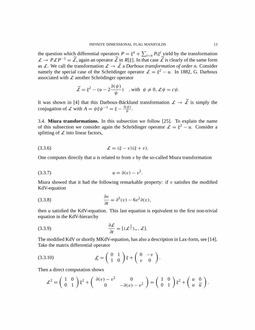
i yield by the transformationL→ PLP−1 = L, again an operator L in R[ξ]. In that case L is clearly of the same formas L. We call the transformation L → L a Darboux transformation of order n. Considernamely the special case of the Schrodinger operator L = ξ2 − u. In 1882, G. Darbouxassociated with L another Schrodinger operator
L = ξ2 − (u− 2∂(ψ)
ψ) , with ψ �= 0,Lψ = cψ.
It was shown in [4] that this Darboux-Backlund transformation L → L is simply theconjugation of L with A = ψξψ−1 = ξ− ∂(ψ)
ψ.
3.4. Miura transformations. In this subsection we follow [25]. To explain the nameof this subsection we consider again the Schrodinger operator L = ξ2 − u. Consider asplitting of L into linear factors,
L = (ξ− v)(ξ+ v).(3.3.6)
One computes directly that u is related to from v by the so-called Miura transformation
u = ∂(v)− v2.(3.3.7)
Miura showed that it had the following remarkable property: if v satisfies the modifiedKdV-equation
∂v
∂t= ∂3(v)− 6v2∂(v),(3.3.8)
then u satisfied the KdV-equation. This last equation is equivalent to the first non-trivialequation in the KdV-hierarchy
∂L
∂t= [(L
32 )+,L].(3.3.9)
The modified KdV or shortly MKdV-equation, has also a description in Lax-form, see [14].Take the matrix differential operator
L =(
0 11 0
)ξ+
(0 −v
v 0
).(3.3.10)
Then a direct computation shows
L2 =(
1 00 1
)ξ2 +
(∂(v)− v2 0
0 −∂(v)− v2
)=
(1 00 1
)ξ2 +
(u 0o u
).
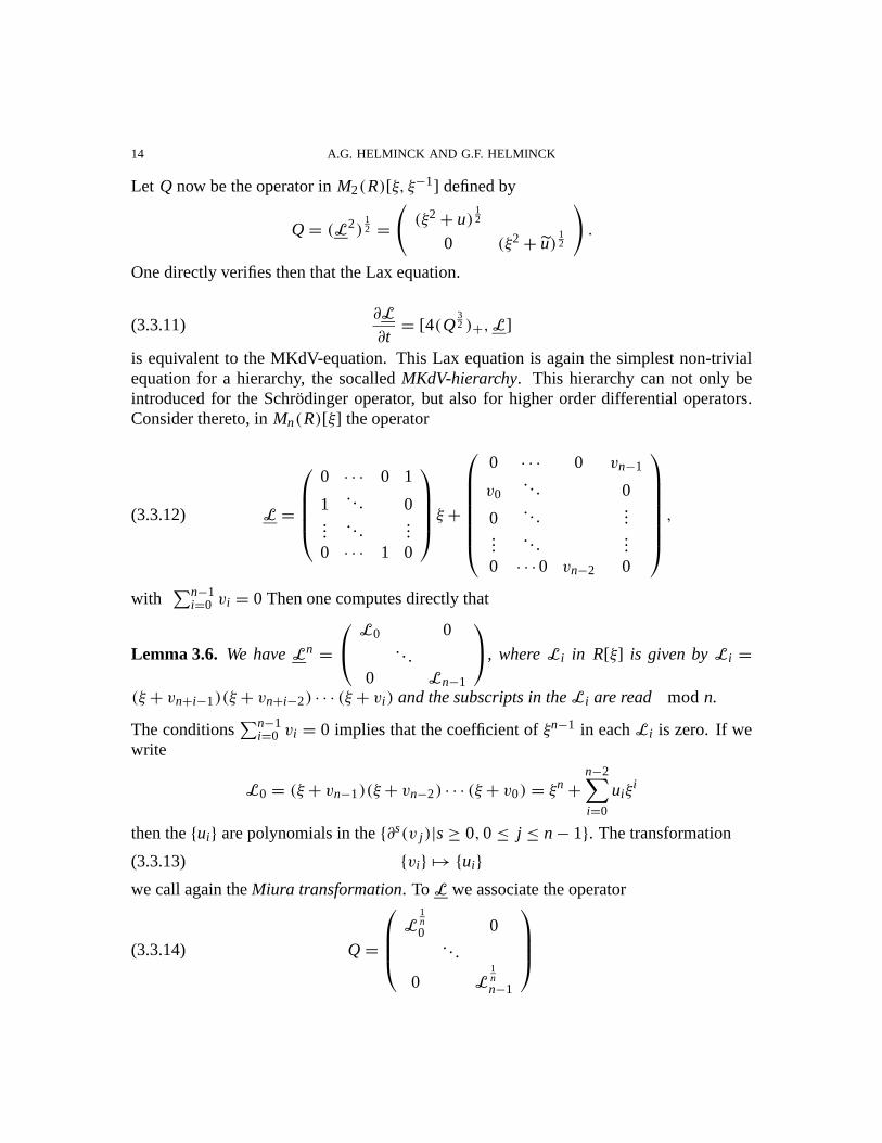
14 A.G. HELMINCK AND G.F. HELMINCK
Let Q now be the operator in M2(R)[ξ, ξ−1] defined by
Q = (L2)12 =
((ξ2 + u)
12
0 (ξ2 + u)12
).
One directly verifies then that the Lax equation.
∂L
∂t= [4(Q
32 )+,L](3.3.11)
is equivalent to the MKdV-equation. This Lax equation is again the simplest non-trivialequation for a hierarchy, the socalled MKdV-hierarchy. This hierarchy can not only beintroduced for the Schrodinger operator, but also for higher order differential operators.Consider thereto, in Mn(R)[ξ] the operator
L =
0 · · · 0 1
1. . . 0
.... . .
...0 · · · 1 0
ξ+
0 · · · 0 vn−1
v0. . . 0
0. . .
......
. . ....
0 · · · 0 vn−2 0
,(3.3.12)
with∑n−1
i=0 vi = 0 Then one computes directly that
Lemma 3.6. We have Ln = L0 0
. . .0 Ln−1
, where Li in R[ξ] is given by Li =
(ξ+ vn+i−1)(ξ+ vn+i−2) · · · (ξ+ vi) and the subscripts in the Li are read mod n.
The conditions∑n−1
i=0 vi = 0 implies that the coefficient of ξn−1 in each Li is zero. If wewrite
L0 = (ξ+ vn−1)(ξ+ vn−2) · · · (ξ+ v0) = ξn +n−2∑i=0
uiξi
then the {ui} are polynomials in the {∂s(v j)|s ≥ 0, 0 ≤ j ≤ n− 1}. The transformation
{vi} �→ {ui}(3.3.13)
we call again the Miura transformation. To L we associate the operator
Q =
L1n0 0
. . .
0 L1nn−1
(3.3.14)
INFINITE DIMENSIONAL FLAG MANIFOLDS 15
in Mn(R)[ξ, ξ−1]. For each k ≥ 1, we consider the Lax equation
∂
∂tkL = [(Qk )+,L].(3.3.15)
We call this the k-th equation of the n-th MKdV-hierarchy and the operator L that satisfiesall these equations is called a solution of this hierarchy. Since (3.3.15) also holds forarbitrary powers of a solution, we see that we have
Proposition 3.7. The Miura transformation maps solutions of the n-th MKdV-hierarchy tosolutions of the n-th KdV-hierarchy.
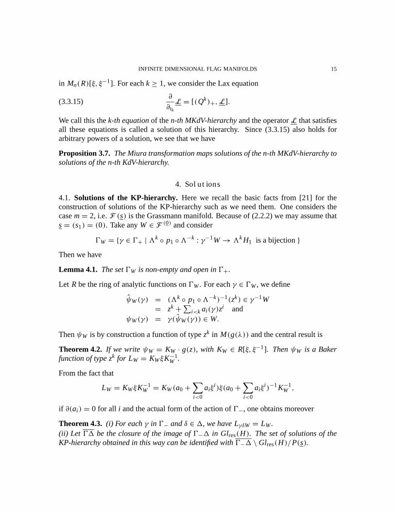
4. Solutions
4.1. Solutions of the KP-hierarchy. Here we recall the basic facts from [21] for theconstruction of solutions of the KP-hierarchy such as we need them. One considers thecase m = 2, i.e. F (s) is the Grassmann manifold. Because of (2.2.2) we may assume thats = (s1) = (0). Take any W ∈ F (0) and consider
�W = {γ ∈ �+ | �k ◦ p1 ◦�−k : γ−1W → �k H1 is a bijection }Then we have
Lemma 4.1. The set �W is non-empty and open in �+.
Let R be the ring of analytic functions on �W . For each γ ∈ �W , we define
ψW (γ) = (�k ◦ p1 ◦�−k )−1(zk ) ∈ γ−1W= zk +∑
i<k ai(γ)zi andψW (γ) = γ(ψW (γ)) ∈ W.
Then ψW is by construction a function of type zk in M(g(λ)) and the central result is
Theorem 4.2. If we write ψW = KW · g(z), with KW ∈ R[ξ, ξ−1]. Then ψW is a Bakerfunction of type zk for LW = KWξK−1
W .
From the fact that
LW = KWξK−1W = KW (a0 +
∑i<0
aiξi)ξ(a0 +
∑i<0
aiξi)−1 K−1
W ,
if ∂(ai) = 0 for all i and the actual form of the action of �−, one obtains moreover
Theorem 4.3. (i) For each γ in �− and δ ∈ �, we have LγδW = LW.(ii) Let �� be the closure of the image of �−� in Glres(H). The set of solutions of theKP-hierarchy obtained in this way can be identified with �−� \ Glres(H)/P(s).
16 A.G. HELMINCK AND G.F. HELMINCK
That � acts trivially on the solutions shows that each connected component of F (0) ren-ders the same set of solutions of the KP-hierarchy. On the other hand the triviality of the�−-action tells you that the commuting flows from �+ give you practically a maximal setof independent directions.One can also characterize geometrically the solutions from 4.2 that correspond to solutionsof the n-th KdV-hierarchy.
Theorem 4.4. For each W ∈ F (0) the following properties are equivalent
(i) (LnW )+ = Ln
W.(ii) �nW ⊂ W.
Proof. (i) ⇒ (ii)If (Ln
W )+ = LnW , then we have
∂n(ψW )(γ) = znψW (γ) for all γ ∈ �W .
Since the {ψW (γ) | γ ∈ �W } are dense in W and the left hand side of this equation belongsto W , we get �nW ⊂ W .(ii) ⇒ (i)For the Baker function ψW we have assume W ∈ F (0)(−k)
∂n(ψW ) = {∂n(KW )K−1W + Ln
W } · ψW
= zn · ψW + ∂n(KW )K−1W · ψW = (Ln
W )+ · ψw
If ∧nW ⊂ W , then we know that znψW (γ) ∈ W . This implies ∂n(Kw) · g(z) ∈ W ∩(γ(zk H1)⊥ = {0} and hence (Ln
W )ψW = (LnW )+ψW . This gives the required equality.
4.2. Darboux transforms. We start with the fundamental observation that shows howflags make their appearance in this framework.
Theorem 4.5. Let W1 and W2 be elements of F (0) belonging to respectively F (0)(m) andF (0)(m+n), with n ≥ 1. Then the following 2 points are equivalent:
(i) There is a polynomial P in R[ξ] of order n such that P · ψW2 = ψW1 .(ii) W1 ⊂ W2.
Proof. (i) ⇒ (ii) for each γ in �W1 ∩ �W2 the vector (P ·ψW2 )(γ) belongs by constructionto W2. Since the vectors
{ψW1 (γ) | γ ∈ �W1 ∩ �W2}are dense in W1, we see that the equality in (i) implies that W1 ⊂ W2.(ii)⇒ (i) As we have seen at the construction of the wavefunctions we have for each i ≥ 0.
ξi · ψW2 (γ) = {z−m−n+i +∑
j<−m−n+i
a j(γ)z j}g(z) and
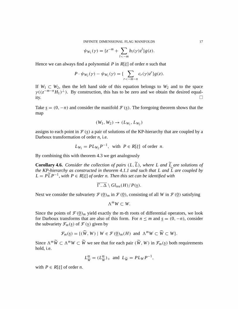
INFINITE DIMENSIONAL FLAG MANIFOLDS 17
ψW1 (γ) = {z−m +∑
l<−m
bl(γ)zl}g(z).
Hence we can always find a polynomial P in R[ξ] of order n such that
P · ψW2 (γ)− ψW1 (γ) = {∑
r<−m−n
cr(γ)zr}g(z).
If W1 ⊂ W2, then the left hand side of this equation belongs to W2 and to the spaceγ((z−m−n H1)⊥). By construction, this has to be zero and we obtain the desired equal-ity.
Take s = (0,−n) and consider the manifold F (s). The foregoing theorem shows that themap
(W1, W2) → (LW1, LW2 )
assigns to each point in F (s) a pair of solutions of the KP-hierarchy that are coupled by aDarboux transformation of order n, i.e.
LW1 = PLW2 P−1, with P ∈ R[ξ] of order n.
By combining this with theorem 4.3 we get analogously
Corollary 4.6. Consider the collection of pairs (L, L), where L and L are solutions ofthe KP-hierarchy as constructed in theorem 4.1.1 and such that L and L are coupled byL = PLP−1, with P ∈ R[ξ] of order n. Then this set can be identified with
�−� \ Glres(H)/P(s).
Next we consider the subvariety F (0)m in F (0), consisting of all W in F (0) satisfying
�mW ⊂ W.
Since the points of F (0)m yield exactly the m-th roots of differential operators, we lookfor Darboux transforms that are also of this form. For n ≤ m and s = (0,−n), considerthe subvariety Fm(s) of F (s) given by
Fm(s) = {(W, W ) | W ∈ F (0)m(H) and �mW ⊂ W ⊂ W}.Since �mW ⊂ �mW ⊂ W we see that for each pair (W, W ) in Fm(s) both requirementshold, i.e.
LmW= (Lm
W)+ and LW = PLW P−1,
with P ∈ R[ξ] of order n.
18 A.G. HELMINCK AND G.F. HELMINCK
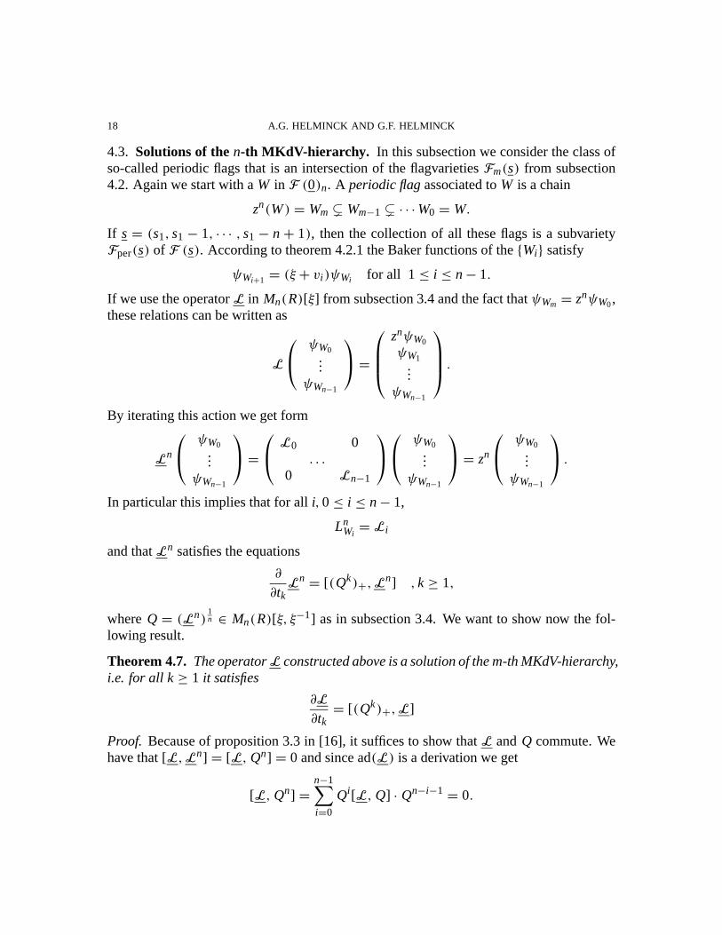
4.3. Solutions of the n-th MKdV-hierarchy. In this subsection we consider the class ofso-called periodic flags that is an intersection of the flagvarieties Fm(s) from subsection4.2. Again we start with a W in F (0)n. A periodic flag associated to W is a chain
zn(W ) = Wm � Wm−1 � · · ·W0 = W.
If s = (s1, s1 − 1, · · · , s1 − n + 1), then the collection of all these flags is a subvarietyFper(s) of F (s). According to theorem 4.2.1 the Baker functions of the {Wi} satisfy
ψWi+1 = (ξ+ vi)ψWi for all 1 ≤ i ≤ n− 1.
If we use the operator L in Mn(R)[ξ] from subsection 3.4 and the fact that ψWm = znψW0 ,these relations can be written as
L
ψW0...
ψWn−1
=
znψW0
ψW1...
ψWn−1
.
By iterating this action we get form
Ln
ψW0...
ψWn−1
= L0 0
. . .
0 Ln−1
ψW0...
ψWn−1
= zn
ψW0...
ψWn−1
.
In particular this implies that for all i, 0 ≤ i ≤ n− 1,
LnWi= Li
and that Ln satisfies the equations
∂
∂tkLn = [(Qk )+,Ln] , k ≥ 1,
where Q = (Ln)1n ∈ Mn(R)[ξ, ξ−1] as in subsection 3.4. We want to show now the fol-
lowing result.
Theorem 4.7. The operator L constructed above is a solution of the m-th MKdV-hierarchy,i.e. for all k ≥ 1 it satisfies
∂L
∂tk= [(Qk)+,L]
Proof. Because of proposition 3.3 in [16], it suffices to show that L and Q commute. Wehave that [L,Ln] = [L, Qn] = 0 and since ad(L) is a derivation we get
[L, Qn] =n−1∑i=0
Qi[L, Q] · Qn−i−1 = 0.
INFINITE DIMENSIONAL FLAG MANIFOLDS 19
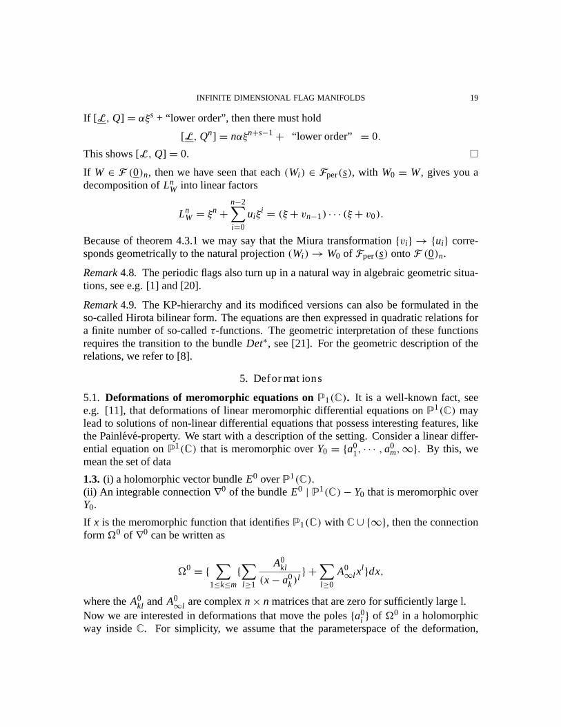
If [L, Q] = αξs + “lower order”, then there must hold
[L, Qn] = nαξn+s−1 + “lower order” = 0.
This shows [L, Q] = 0.
If W ∈ F (0)n, then we have seen that each (Wi) ∈ Fper(s), with W0 = W , gives you adecomposition of Ln
W into linear factors
LnW = ξn +
n−2∑i=0
uiξi = (ξ+ vn−1) · · · (ξ+ v0).
Because of theorem 4.3.1 we may say that the Miura transformation {vi} → {ui} corre-sponds geometrically to the natural projection (Wi) → W0 of Fper(s) onto F (0)n.
Remark 4.8. The periodic flags also turn up in a natural way in algebraic geometric situa-tions, see e.g. [1] and [20].
Remark 4.9. The KP-hierarchy and its modificed versions can also be formulated in theso-called Hirota bilinear form. The equations are then expressed in quadratic relations fora finite number of so-called τ-functions. The geometric interpretation of these functionsrequires the transition to the bundle Det∗, see [21]. For the geometric description of therelations, we refer to [8].
5. Deformations
5.1. Deformations of meromorphic equations on �1(�). It is a well-known fact, seee.g. [11], that deformations of linear meromorphic differential equations on �1(�) maylead to solutions of non-linear differential equations that possess interesting features, likethe Painleve-property. We start with a description of the setting. Consider a linear differ-ential equation on �1(�) that is meromorphic over Y0 = {a0
1, · · · , a0m,∞}. By this, we
mean the set of data
1.3. (i) a holomorphic vector bundle E0 over �1(�).(ii) An integrable connection ∇0 of the bundle E0 | �1(�)− Y0 that is meromorphic overY0.
If x is the meromorphic function that identifies �1(�) with � ∪ {∞}, then the connectionform �0 of ∇0 can be written as
�0 = {∑
1≤k≤m
{∑l≥1
A0kl
(x− a0k )l} +
∑l≥0
A0∞l x
l}dx,
where the A0kl and A0
∞l are complex n× n matrices that are zero for sufficiently large l.Now we are interested in deformations that move the poles {a0
i } of �0 in a holomorphicway inside �. For simplicity, we assume that the parameterspace of the deformation,
20 A.G. HELMINCK AND G.F. HELMINCK
shortly called deformation space, is a connected complex variety T. The way the polesare moved is determined by a set of holomorphic functions ai : T → �, 1 ≤ i ≤ m, the so-called deformation functions. Furthermore there has to be a base point t0 in T such thatai(t0) = a0
i for all i. To avoid a priori topological obstructions, we will restrict ourselvesto deformations for which the poles never coincide, i.e. the deformation functions satisfy
ai(t) �= a j(t) for all t in T and all i �= j.
Let X be �1(�)× T . We can introduce a smooth codimension one subvariety Y of X by
Y = Y1 ∪ . . . ∪ Ym ∪ Y∞ with
Yi = {(x, t) | (x, t) ∈ X, x = ai(t)} and Y∞ = {(∞, t) | (∞, t) ∈ X}.The object one is interested in, is then
Definition 5.1. An integrable deformation (E,∇) of the pair (E0,∇0) with deformationspace T , deformation functions {ai} and base point t0 in T consists of
(i) a holomorphic vector bundle E over X = �1(�)× T of rank n.(ii) an integrable connection ∇ of E | X − Y , that is meromorphic over Y and that is suchthat the restriction of (E,∇) to �1(�)× {t0} is isomorphic to (E0,∇0).
Given the deformation space, the deformation functions {ai} and the base point {t0}, arelevant question is if there exists an integrable deformation with these deformation data.Even if there is no fusion of the poles, one might hit at topological obstructions. Leti : �1(�) → T be the embedding x �→ (x, t0). It induces a natural map i∗ : π1(�1(�)−Y0) → π1(X − Y ). If there exists an integrable deformation (E,∇) of (E0,∇0), thenthe representation ρ of π1(�1(�) − {a0
1, . . . , a0m,∞}) corresponding to (E0,∇0) has to
factorize through i∗. Consider the projection p2 : X− Y → T , given by p2((x, t)) = t. Thefiber over t is equal to �− {a1(t), . . . , am(t)}. Thus (X − Y, T, p2) is a fiber bundle andwe have the long exact sequence
π2(T ) → π1(�1(�)− {a01, . . . , a0
m,∞}) i∗−→ π1(X − Y ) → π1(T ) → 1.
Now ρ has to be trivial on the image of π2(T ) and should be extendable to π1(X − Y ).Such problems do not occur if π2(T ) = π1(T ) = {1}. In that case the monodromy ispreserved by the deformation. An example of such a deformation space occurred in [5]and is given by
Example 5.2. Let Z be the space
Z = �m −⋃i �= j
Dij, where Dij = {(xk ) ∈ �m, xi = x j}.
INFINITE DIMENSIONAL FLAG MANIFOLDS 21
As deformation space we take the universal covering space Z of Z and for ai : Z → � wetake the composition of the natural projection π : Z → Z with the projection on the i-thcoordinate.
Remark 5.3. From the construction one sees directly that in a neighbourhood of the singu-lar point (a0
j , t0) ∈ Yj, the singular part of the connection form � has w.r.t. any trivializingbasis of local sections of E, the form∑
l≥1
B jl(t)
(x− a j(t))ld(x− a j),
where all the B jl are holomorphic. By applying a proper coordinate transformation, onemay moreover assume
B jl(t0) = A jl(t0) for all l.
Since we considered integrable deformations the functions B jl satisfy the non-linear com-patibility conditions and those are the non-linear equations we refered to at the beginning.E.g., if ∇0 has a logarithmic pole over Y0, i.e. A0
kl = 0 for all l > 1 and A0∞l = 0 for all
l ≥ 0, then the B j1 satisfy the so-called “Schlesinger equations”
dBi1 = −∑j �=i
[Bi1, B j1]d(ai − a j)
ai − a j.
For the space Z with the deformation functions {ai} as in the foregoing example we had notopological obstructions and this turns out to be sufficient, for following carefully the linesof proof in [15], one can show
Theorem 5.4. For each pair (E0,∇0) there exists an integrable deformation (E,∇) of(E0,∇0) with Z as deformation space and the {ai} as deformation functions.
Let (E,∇) be the integrable deformation from theorem 5.4. and assume E0 was a trivialvector bundle. Then we consider as in [15], the set
� = {t ∈ Z|E|�1(�)×{t} is non-trivial}Since all holomorphic line bundles over Z are trivial, one can show
Proposition 5.5. There is a holomorphic τ : Z → � such that
� = {t ∈ Z, τ(t) = 0}.Choose open balls D1 and D2 in �1(�) such that D1 ∪ D2 = �1(�) and that E|D1 × Zand E|D2 × Z are trivial. The comparison of trivializing sections of these two bundles,gives you a holomorphic transfer funtion
S : D1 ∩ D2 × Z → Gln(�).
22 A.G. HELMINCK AND G.F. HELMINCK
Let H be L2(S1, �n) with the decomposition H = H+ ⊕ H⊥+ , where
H+ = {∑i≥0
bixi ∈ H, bi ∈ �n}.
Then S determines a holomorphic family of operators {�(t)|t ∈ Z} in Glres(H), such that�(t) is in the big cell for all t ∈ Z −�. Locally one can fit the �(t) into the group G andthis suffices to prove that
Proposition 5.6. (i) There exist holomorphic maps S+ : D2 × { Z −�} → Gln(�) andS− : D1 × { Z −�} → Gln(�) with S−(∞, t) = Id such that S = S−1− S+.(ii) The maps S+ and S− are meromorphic over D2 ×� resp. D1 ×�.
In the case that ∇0 has a logarithmic pole at infinity this proposition is used to show thatthe connection form of ∇|Di × Z − Y ∩ {Di × Z} w.r.t. suitable trivializing basis extendsmeromorphically to Di × Z. Thus one obtains the following result.
Theorem 5.7. (i) Assume that E0 is trivial and that ∇0 has a logarithmic pole at infinity. Let (E,∇) be the integrable deformation from 5.4. Then there is a neighbourhood U oft0 such that E | �1(�)×U is trivial and a basis of sections {hi} such that the connectionform � w.r.t. the {hi} looks like
� =m∑
i=1
∑l≥1
Bil(t)
(x− ai(t))ld(x− ai),
with Bil(t0) = A0il for all i and l.
(ii) These solutions {Bil} of the integrability equations extend holomorphically to Z −�
and are meromorphic on Z.
Remark 5.8. In the case that ∇0 has logarithmic poles over Y0, Malgrange has shown in[15] that there is a holomorphic τ : Z → � with zero-set � such that ω = dτ
τis the differ-
ential form presented in [11]. This τ-function can also be interpreted as the determinant ofan associated Cauchy-Riemann operator on the spin bundle over �1(�), see [17].
Remark 5.9. The bundle Det∗ plays also an important role at monodromy preserving de-formations of Dirac equations, see [18] and [19].
References
[1] M. Adler, L. Haine, P. van Moerbeke, Limit matrices for the Toda flow and periodic flags for loopgroups, preprint.
[2] R.J. Baston, M.G. Eastwood, The Penrose transform, Clarendon Press, Oxford 1989.[3] A.L. Carey, S.N.M. Ruysenaars, On Fermion Gauge Groups, Current Algebras and Kac-Moody alge-
bras, Acta Appl. Math, 1987, p. 1-86.
INFINITE DIMENSIONAL FLAG MANIFOLDS 23
[4] F. Ehlers, H. Knorrer, An algebro-geometric interpretation of the Backlund transformation for theKorteweg-de Vries equation, Comment. Math. Helvetici 57 (1982), 1–10.
[5] M. Fukuma, H. Kawai, R. Nakayama, Infinite Dimensional Grassmannian Structure of Two-Dimensional Quantum Gravity, Commun. Math. Phys. 143, p. 371-403 (1992).
[6] L. Haine, E. Horozov, Toda orbits of Laguerre polynomials and representations of the Virasoro algebra,Bull. Sc. Math, 2e serie 117, 1993, p. 485-518.
[7] G. Helminck, A geometric construction of solutions of the Toda lattice hierarchy, Lecture Notes inPhysics, 424, p. 91-101.
[8] G.F. Helminck, A.G. Helminck, The structure of Hilbert flag varieties, to appear in Publ. RIMS, KyotoUniversity.
[9] M. Hazewinkel, C.F. Martin,Representations of the symmetric group the specialization order, Systemsand Grassmann manifolds, l’Enseignement Mathematique, 29 (1983), 53–87.
[10] G.F. Helminck, G.F. Post, The geometry of differential difference equations, to appear in IndagationesMathematicae.
[11] M. Jimbo, T. Muire and K. Ueno, Monodromy preserving deformations of linear ordinary differentialequations with rational coefficients 1. General theory and τ-functions, Phys 2D 402 (1981), p. 306-352.
[12] N. Kawamoto, Y. Narukawa, A. Tsychiya, Y. Yamada, Geometric Realization of Conformal Field The-ory on Riemann Surfaces, Commun. Math. Phys. 116, p. 247-308 (1988).
[13] V.G. Kac, D.H. Peterson, Infinite flag varieties and conjugacy theorems, Proc. Nat. Acad. Sci. USA, 18(1983), 1778–1782.
[14] B.A. Kupershmidt, G. Wilson, Modifying Lax equations and the second Hamiltonian structure, Invent.Math. 62 (1981), 403–436.
[15] B. Malgrange, Sur les deformations isomonodromiques 1. Singularites reguliers, Progress in Mathe-matics, vol 37 (Birkhauser, Boston, 1983).
[16] J. Mickelsson, Current Algebras and Groups, Plenum Monographs in Nonlinear Physics, Plenum Press,New York (1989).
[17] J. Palmer, Determinants of Cauchy Riemann operators as τ-functions, Acta Appl. Math. 18, No. 3(1990), 199–223.
[18] J. Palmer, Tau functions for the Dirac operator in the Euclidean plane, Pacific Journal of Mathematics,vol 160, no. 2 (1993), 259–342.
[19] J. Palmer, M. Beatty, C.A. Tracy, Tau functions for the Dirac operator on the Poincare disk, preprint.[20] A. Pressley, G. Segal, Loop groups, Clarendon Press, Oxford 1986.[21] G. Segal, G. Wilson, Loop groups and equations of KdV-type, Publ. Math. IHES 61, (1985), 5–65.[22] R.S. Ward, R.O. Wells jr., Twistor Geometry and Field Theory, Cambridge Monographs on Mathemat-
ical Physics, University Press, Cambridge (1991).[23] G. Wilson, Commuting flows and conservation laws for Lax equations, Math. Proc. Cambridge Philos.
Soc. 86 (1979), 131–143.[24] G. Wilson, Habillage et fonctions τ, C.R. Acad. Sci, Paris Ser. I. Math. 299 (1984), 587–590.[25] G. Wilson, Loop groups and equations of KdV type II, Flag manifolds and the modified equations,
preprint.[26] W. Witten, Quantum Field Theory, Grassmannian and Algebraic Curves, Commun. Math. Phys. 113,
p. 539–600 (1988).
24 A.G. HELMINCK AND G.F. HELMINCK
Department of Mathematics, North Carolina State University, Raleigh, N.C., 27695-8205E-mail address: [email protected]
Department of Mathematics, Universiteit Twente, Enschede, The NetherlandsE-mail address: [email protected]


![arXiv:math/0107201v2 [math.SG] 23 Jan 2002 · 2018. 10. 30. · We strongly suspect that there are preciously few manifolds that admit toric integrable geodesic flows. In fact the](https://img.pdfslide.us/doc/110x75/6083ef5bf8ec900ce43c2855/arxivmath0107201v2-mathsg-23-jan-2002-2018-10-30-we-strongly-suspect-that.jpg)