Embed Size (px)
Citation preview

Inferring team task plans from human meetings: Agenerative modeling approach with logic-based prior
Citation Kim, Been, Caleb M. Chacha, and Julie A. Shah. "Inferring teamtask plans from human meetings: A generative modelingapproach with logic-based prior." Journal of Artificial IntelligenceResearch 52 (2015): 361-398. © 2015 AI Access Foundation
As Published http://dx.doi.org/10.1613/jair.4496
Publisher Association for the Advancement of Artificial Intelligence
Version Final published version
Accessed Wed Mar 02 13:13:05 EST 2016
Citable Link http://hdl.handle.net/1721.1/97138
Terms of Use Article is made available in accordance with the publisher's policyand may be subject to US copyright law. Please refer to thepublisher's site for terms of use.
Detailed Terms
The MIT Faculty has made this article openly available. Please sharehow this access benefits you. Your story matters.
Journal of Artificial Intelligence Research 52 (2015) 361-398 Submitted 7/14; published 3/15
Inferring Team Task Plans from Human Meetings:A Generative Modeling Approach with Logic-Based Prior
Been Kim [email protected]
Caleb M. Chacha c [email protected]
Julie A. Shah julie a [email protected]
Massachusetts Institute of Technology
77 Massachusetts Ave. MA 02139, USA
Abstract
We aim to reduce the burden of programming and deploying autonomous systems towork in concert with people in time-critical domains such as military field operations anddisaster response. Deployment plans for these operations are frequently negotiated on-the-fly by teams of human planners. A human operator then translates the agreed-upon planinto machine instructions for the robots. We present an algorithm that reduces this transla-tion burden by inferring the final plan from a processed form of the human team’s planningconversation. Our hybrid approach combines probabilistic generative modeling with logicalplan validation used to compute a highly structured prior over possible plans, enabling usto overcome the challenge of performing inference over a large solution space with only asmall amount of noisy data from the team planning session. We validate the algorithmthrough human subject experimentations and show that it is able to infer a human team’sfinal plan with 86% accuracy on average. We also describe a robot demonstration in whichtwo people plan and execute a first-response collaborative task with a PR2 robot. To thebest of our knowledge, this is the first work to integrate a logical planning technique withina generative model to perform plan inference.
1. Introduction
Robots are increasingly being introduced to work in concert with people in high-intensitydomains such as military field operations and disaster response. For example, robot deploy-ment can allow for access to areas that would otherwise be inaccessible to people (Casper& Murphy, 2003; Micire, 2002), to inform situation assessment (Larochelle, Kruijff, Smets,Mioch, & Groenewegen, 2011). The human-robot interface has long been identified as a ma-jor bottleneck in utilizing these robotic systems to their full potential (Murphy, 2004). As aresult, significant research efforts have been aimed at easing the use of these systems in thefield, including careful design and validation of supervisory and control interfaces (Jones,Rock, Burns, & Morris, 2002; Cummings, Brzezinski, & Lee, 2007; Barnes, Chen, Jentsch,& Redden, 2011; Goodrich, Morse, Engh, Cooper, & Adams, 2009). Much of this priorwork has focused on ease of use at “execution time.” However, a significant bottleneck alsoexists in planning the deployment of autonomous systems and in the programming of thesesystems to coordinate task execution with a human team. Deployment plans are frequentlynegotiated by human team members on-the-fly and under time pressure (Casper & Murphy,2002, 2003). For a robot to aid in the execution of such a plan, a human operator musttranscribe and translate the result of a team planning session.
c©2015 AI Access Foundation. All rights reserved.
Kim, Chacha & Shah
In this paper, we present an algorithm that reduces this translation burden by inferringthe final plan from a processed form of the human team’s planning conversation. Inferringthe plan from noisy and incomplete observation can be formulated as a plan recognitionproblem (Ryall, Marks, & Shieber, 1997; Bauer, Biundo, Dengler, Koehler, & Paul, 2011;Mayfield, 1992; Charniak & Goldman, 1993; Carberry, 1990; Grosz & Sidner, 1990; Gal,Reddy, Shieber, Rubin, & Grosz, 2012). The noisy and incomplete characteristics of obser-vation stem from the fact that not all observed data (e.g., the team’s planning conversation)will be a part of the plan that we are trying to infer, and that the entire plan may not beobserved. The focus of existing plan recognition algorithms is often to search an existingknowledge base given noisy observation. However, deployment plans for emergency situ-ations are seldom the same, making it infeasible to build a knowledge base. In addition,planning conversations are often conducted under time pressure and are, therefore, oftenshort (i.e., contain a small amount of data). Shorter conversations result in a limited amountof available data for inference, often making the inference problem more challenging.
Our approach combines probabilistic generative modeling with logical plan validation,which is used to compute a highly structured prior over possible plans. This hybrid approachenables us to overcome the challenge of performing inference over a large solution space withonly a small amount of noisy data collected from the team planning session.
In this work, we focus on inferring a final plan using text data that can be logged fromchat or transcribed speech. Processing human dialogue into more machine-understandableforms is an important research area (Kruijff, Janıcek, & Lison, 2010; Tellex, Kollar, Dick-erson, Walter, Banerjee, Teller, & Roy, 2011; Koomen, Punyakanok, Roth, & Yih, 2005;Palmer, Gildea, & Xue, 2010; Pradhan, Ward, Hacioglu, Martin, & Jurafsky, 2004), but weview this as a separate problem and do not focus on it in this paper.
The form of input we use preserves many of the challenging aspects of natural humanplanning conversations, and can be thought of as noisy observation of the final plan. Becausethe team is discussing the plan under time pressure, planning sessions often consist of asmall number of succinct communications. Our approach can infer the final agreed-uponplan using a single planning session, despite a small amount of noisy data.
We validate the algorithm through experiments with 96 human subjects and show thatwe are able to infer a human team’s final plan with 86% accuracy on average. To the bestof our knowledge, this is the first work to integrate a logical planning technique within agenerative model to perform plan inference.
In summary, this work includes the following contributions:
• We formulate the novel problem of performing inference to extract a finally agreed-upon plan from a human team planning conversation.
• We propose and validate a hybrid approach to perform this inference that appliesthe logic-based prior probability over the space of possible agreed-upon plans. Thisapproach performs efficient inference for the probabilistic generative model.
• We demonstrate the benefit of this approach using human team meeting data collectedfrom large-scale human subject experiments (total 96 subjects) and are able to infera human team’s final plan with 86% accuracy on average.
362
A Generative Modeling Approach with Logic-Based Prior
This work extends the preliminary version of this work (Kim, Chacha, & Shah, 2013) toinclude the inference of complex durative task plans and to infer plans before and after newinformation becomes available for the human team. In addition, we extend our probabilisticmodel to be more flexible to different data sets by learning hyper-parameters. We alsoimprove the performance of our algorithm by designing a better proposal distribution forinference.
The formulation of the problem is presented in Section 2, followed by the technicalapproach and related work in Section 3. Our algorithm is described in Section 4. Theevaluation of the algorithm using various data sets is shown in Sections 5 and 6. Finally,we discuss the benefits and limitations of the current approach in Section 7, and concludewith considerations for future work in Section 8.
2. Problem Formulation
Disaster response teams are increasingly utilizing web-based planning tools to plan deploy-ments (Di Ciaccio, Pullen, & Breimyer, 2011). Hundreds of responders access these toolsto develop their plans using audio/video conferencing, text chat and annotatable maps.Rather than working with raw, natural language, our algorithm takes a structured form ofthe human dialogue from these web-based planning tools as input. The goal of this workis to infer a human team’s final plan from this human dialogue. In doing so, this work canbe used to design an intelligent agent for these planning tools that can actively participateduring a planning session to improve the team’s decision.
This section describes the formal definition, input and output of the problem. Formally,this problem can be viewed as one of plan recognition, wherein the plan follows the formalrepresentation of the Planning Domain Description Language (PDDL). The PDDL hasbeen widely used in the planning research community and planning competitions (i.e., theInternational Planning Competition). A plan is valid if it achieves a user-specified goal statewithout violating user-specified plan constraints. Actions may be constrained to executein sequence or in parallel with other actions. Other plan constraints can include discreteresource constraints (e.g. the presence of two medical teams) and temporal deadlines fortime-durative actions (e.g. a robot can only be deployed for up to 1 hour at a time due tobattery life constraints).
We assume that the team reaches agreement on a final plan. The techniques introducedby Kim and Shah (2014) can be used to detect the strength of this agreement, and toencourage the team to further discuss the plan to reach an agreement if necessary. Situationswhere a team agrees upon a flexible plan with multiple options to be explored will beincluded in future study. Also, while we assume that the team is more likely to agree on avalid plan, we do not rule out the possibility that the final plan is invalid.
2.1 Algorithm Input
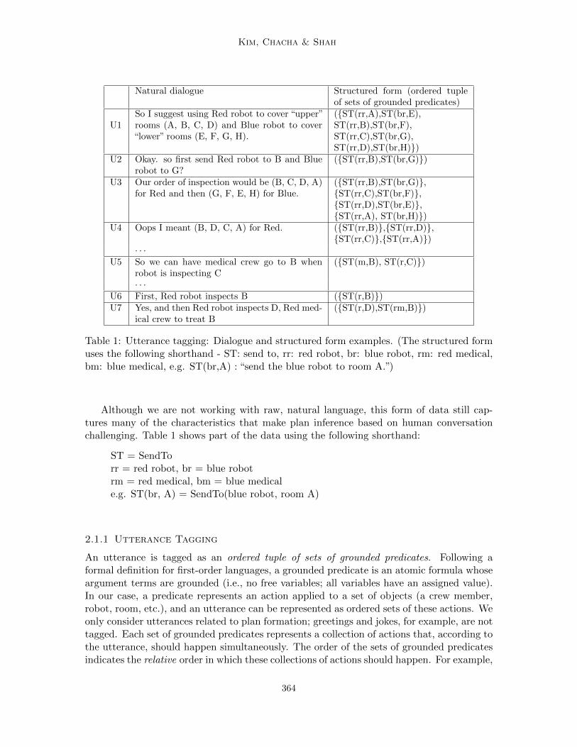
Text data from the human team conversation is collected in the form of utterances, whereeach utterance is one person’s turn in the discussion, as shown in Table 1. The input to ouralgorithm is a machine-understandable form of human conversation data, as illustrated inthe right-hand column of Table 1. This structured form captures the actions discussed andthe proposed ordering relations among actions for each utterance.
363
Kim, Chacha & Shah
Natural dialogue Structured form (ordered tupleof sets of grounded predicates)
U1So I suggest using Red robot to cover “upper”rooms (A, B, C, D) and Blue robot to cover“lower” rooms (E, F, G, H).
({ST(rr,A),ST(br,E),ST(rr,B),ST(br,F),ST(rr,C),ST(br,G),ST(rr,D),ST(br,H)})
U2 Okay. so first send Red robot to B and Bluerobot to G?
({ST(rr,B),ST(br,G)})
U3 Our order of inspection would be (B, C, D, A)for Red and then (G, F, E, H) for Blue.
({ST(rr,B),ST(br,G)},{ST(rr,C),ST(br,F)},{ST(rr,D),ST(br,E)},{ST(rr,A), ST(br,H)})
U4 Oops I meant (B, D, C, A) for Red. ({ST(rr,B)},{ST(rr,D)},{ST(rr,C)},{ST(rr,A)})
· · ·U5 So we can have medical crew go to B when
robot is inspecting C({ST(m,B), ST(r,C)})
· · ·U6 First, Red robot inspects B ({ST(r,B)})U7 Yes, and then Red robot inspects D, Red med-
ical crew to treat B({ST(r,D),ST(rm,B)})
Table 1: Utterance tagging: Dialogue and structured form examples. (The structured formuses the following shorthand - ST: send to, rr: red robot, br: blue robot, rm: red medical,bm: blue medical, e.g. ST(br,A) : “send the blue robot to room A.”)
Although we are not working with raw, natural language, this form of data still cap-tures many of the characteristics that make plan inference based on human conversationchallenging. Table 1 shows part of the data using the following shorthand:
ST = SendTorr = red robot, br = blue robotrm = red medical, bm = blue medicale.g. ST(br, A) = SendTo(blue robot, room A)
2.1.1 Utterance Tagging
An utterance is tagged as an ordered tuple of sets of grounded predicates. Following aformal definition for first-order languages, a grounded predicate is an atomic formula whoseargument terms are grounded (i.e., no free variables; all variables have an assigned value).In our case, a predicate represents an action applied to a set of objects (a crew member,robot, room, etc.), and an utterance can be represented as ordered sets of these actions. Weonly consider utterances related to plan formation; greetings and jokes, for example, are nottagged. Each set of grounded predicates represents a collection of actions that, according tothe utterance, should happen simultaneously. The order of the sets of grounded predicatesindicates the relative order in which these collections of actions should happen. For example,
364
A Generative Modeling Approach with Logic-Based Prior
({ST(rr, B), ST(br, G)}, {ST(rm, B)}) corresponds to sending the red robot to room Band the blue robot to room G simultaneously, followed by sending the red medical team toroom B.
As indicated in Table 1, the structured dialogue still includes high levels of noise. Eachutterance (i.e. U1-U7) discusses a partial plan, and only predicates explicitly mentioned inthe utterance are tagged (e.g. U6-U7: the “and then” in U7 implies a sequencing constraintwith the predicate discussed in U6, but the structured form of U7 does not include ST(r,B)).Typos and misinformation are tagged without correction (e.g. U3), and any utterancesindicating a need to revise information are not placed in context (e.g. U4). Utterances thatclearly violate the ordering constraints (e.g. U1: all actions cannot happen at the sametime) are also tagged without correction. In addition, information regarding whether anutterance was a suggestion, rejection of or agreement with a partial plan is not coded.
Note that the utterance tagging only contains information about relative ordering be-tween the predicates appearing in that utterance, not the absolute ordering of their appear-ance in the final plan. For example, U2 specifies that the two grounded predicates happenat the same time. It does not state when the two predicates happen in the final plan, orwhether other predicates will happen in parallel. This simulates how humans conversationsoften unfold — at each utterance, humans only observe the relative ordering, and inferthe absolute order of predicates based on the whole conversation and an understanding ofwhich orderings would make a valid plan. This utterance tagging scheme is also designedto support the future transition to automatic natural language processing. Automatic se-mantic role labeling (Jurafsky & Martin, 2000), for example, can be used to detect thearguments of predicates from sentences. One of the challenges with incorporating semanticrole labeling into our system is that the dialogue from our experiments is often colloquialand key grammatical components of sentences are often omitted. Solving this problem andprocessing free-form human dialogue into more machine-understandable forms is an impor-tant research area, but we view that as a separate problem and do not focus on it in thispaper.
2.2 Algorithm Output
The output of the algorithm is an inferred final plan, sampled from the probability distri-bution over the final plans. The final plan has the same representation to the structuredutterance tags (ordered tuple of sets of grounded predicates). The predicates in each setrepresent actions that should happen in parallel, and the ordering of sets indicates the se-quence. Unlike the utterance tags, however, the sequence ordering relations in the finalplan represent the absolute order in which the actions are to be carried out. An example ofa plan is ({A1, A2}, {A3}, {A4, A5, A6}), where Ai represents a predicate. In this plan, A1
and A2 will happen at step 1 of the plan, A3 happens at step 2 of the plan, and so on.
3. Approach in a Nutshell and Related Work
Planning conversations performed under time pressure exhibit unique characteristics andchallenges for inferring the final plan. First, these planning conversations are succinct —participants tend to write shortly and briefly, and to be in a hurry to make a final decision.Second, there may be a number of different valid plans for the team’s deployment — even
365

Kim, Chacha & Shah
Figure 1: Web-based tool developed and used for data collection
366
A Generative Modeling Approach with Logic-Based Prior
with a simple scenario, people tend to generate a broad range of final plans. This representsthe typical challenges faced during real rescue missions, where each incident is unique andparticipants cannot have a library of plans to choose from at each time. Third, theseconversations are noisy — often, many suggestions are made and rejected more quicklythan they would be in a more casual setting. In addition, there are not likely to be manyrepeated confirmations of agreement, which might typically ease detection of the agreed-upon plan.
It might seem natural to take a probabilistic approach to the plan inference problem,as we are working with noisy data. However, the combination of a small amount of noisydata and a large number of possible plans means that inference using typical, uninformativepriors over plans may fail to converge to the team’s final plan in a timely manner.
This problem could also be approached as a logical constraint problem of partial orderplanning, if there were no noise in the utterances: If the team were to discuss only partialplans relating to the final plan, without any errors or revisions, then a plan generator orscheduler (Coles, Fox, Halsey, Long, & Smith, 2009) could produce the final plan usingglobal sequencing. Unfortunately, data collected from human conversation is sufficientlynoisy to preclude this approach.
These circumstances provided motivation for a combined approach, wherein we builta probabilistic generative model and used a logic-based plan validator (Howey, Long, &Fox, 2004) to compute a highly structured prior distribution over possible plans. Intuitivelyspeaking, this prior encodes our assumption that the final plan is likely, but not required,to be a valid plan. This approach naturally deals with both the noise in the data andthe challenge of performing inference over plans with only a limited amount of data. Weperformed sampling inference in the model using Gibbs and Metropolis-Hastings samplingto approximate the posterior distribution over final plans, and empirical validation withhuman subject experiments indicated that the algorithm achieves 86% accuracy on average.More details of our model and inference methods are presented in Section 4.
The related work can be categorized into two categories: 1) application and 2) technique.In terms of application, our work relates to plan recognition (Section 3.1). In terms oftechnique, our approach relates to methods that combine logic and probability, thoughwith different focused applications (Section 3.2).
3.1 Plan Recognition
Plan recognition has been an area of interest within many domains, including interactivesoftware (Ryall et al., 1997; Bauer et al., 2011; Mayfield, 1992), story understanding (Char-niak & Goldman, 1993) and natural language dialogue (Carberry, 1990; Grosz & Sidner,1990).
The literature can be categorized in two ways. The first is in terms of requirements.Some studies (Lochbaum, 1998; Kautz, 1987) require a library of plans, while others (Zhuo,Yang, & Kambhampati, 2012; Ramırez & Geffner, 2009; Pynadath & Wellman, 2000;Sadilek & Kautz, 2010) replace this library with relevant structural information. If a libraryof plans is required, some studies (Weida & Litman, 1992; Kautz, Pelavin, Tenenberg, &Kaufmann, 1991) assumed that this library can be collected, and that all future plans areguaranteed to be included within the collected library. By contrast, if a library of plans is
367

Kim, Chacha & Shah
not required, it can be replaced by related structure information, such as a domain theoryor the possible set of actions performable by agents. The second categorization for theliterature is in terms of technical approach. Some studies incorporated constraint-basedapproaches, while others took probabilistic or combination approaches.
First, we reviewed work that treated plan recognition as a knowledge base search prob-lem. This method assumes that you either have or can build a knowledge base, and thatyour goal is to efficiently search this knowledge base (Lochbaum, 1998; Kautz, 1987). Thisapproach often includes strong assumptions regarding the correctness and completeness ofthe plan library, in addition to restrictions on noisy data (Weida & Litman, 1992; Kautzet al., 1991), and is applicable in domains where the same plan reoccurs naturally. Forexample, Gal et al. (2012) studied how to adaptively adjust educational content for a betterlearning experience, given students’ misconceptions, using a computer-based tutoring tool.Similarly, Brown and Burton (1978) investigated users’ underlying misconceptions usinguser data collected from multiple sessions spent trying to achieve the same goal. In termsof technical approach, the above approaches used logical methods to solve the orderingconstraints problem of searching the plan library.
We also reviewed work that replaced a knowledge base with the structural informationof the planning problem. Zhuo et al. (2012) replaced the knowledge base with action modelsof the domain, and formulated the problem as one of satisfiability to recognize multi-agentplans. A similar approach was taken by Ramırez and Geffner (2009), wherein action modelswere used to replace the plan library, while Pynadath and Wellman (2000) incorporatedan extension of probabilistic context free grammars (PCFGs) to encode a set of predefinedactions to improve efficiency. More recently, Markov logic was applied to model the geom-etry, motion model and rules for the recognition of multi-agent plans while playing a gameof capture the flag (Sadilek & Kautz, 2010). Replacing the knowledge base with structuralinformation reduces the amount of prior information required. However, there are two ma-jor issues with the application of prior work to recognize plans from team conversation:First, the above work assumed some repetition of previous plans. For example, learning theweights in Markov logic (which represent the importance or strictness of the constraints)requires prior data from the same mission, with the same conditions and resources. Sec-ond, using first-order logic to express plan constraints quickly becomes computationallyintractable as the complexity of a plan increases.
In contrast to logical approaches, probabilistic approaches allow for noisy observations.Probabilistic models are used to predict a user’s next action, given noisy data (Albrecht,Zuckerman, Nicholson, & Bud, 1997; Horvitz, Breese, Heckerman, Hovel, & Rommelse,1998). These works use actions that are normally performed by users as training data.However, the above approaches do not consider particular actions (e.g., actions that mustbe performed by users to achieve certain goals within a software system) to be more likely.In other words, while they can deal with noisy data, they do not incorporate structuralinformation that could perhaps guide the plan recognition algorithm. An additional limita-tion of these methods is that they assume predefined domains. By defining a domain, theset of possible plans is limited, but the possible plans for time-critical missions is generallynot a limited set. The situation and available resources for each incident are likely to bedifferent. A method that can recognize a plan from noisy observations, and from an openset of possible plans, is required.
368
A Generative Modeling Approach with Logic-Based Prior
Some probabilistic approaches incorporate structure through the format of a plan li-brary. Pynadath and Wellman (2000) represented plan libraries as probabilistic contextfree grammars (PCFGs). Then this was used to build Bayes networks that modeled the un-derlying generative process of plan construction. However, their parsing-based approachesdid not deal with partially-ordered plans or temporally interleaved plans. Geib et al. (2008)and Geib and Goldman (2009) overcame this issue by working directly with the plan repre-sentation without generating an intermediate representation in the form of a belief network.At each time step, their technique observed the previous action of the agent and generateda pending action set. This approach, too, assumed an existing plan library and relied onthe domains with some repetition of previous plans. More recently, Nguyen, Kambhampati,and Do (2013) introduced techniques to address incomplete knowledge of the plan library,but for plan generation rather than plan recognition applications.
Our approach combines a probabilistic approach with logic-based prior to infer teamplans without the need for historical data, using only situational information and data froma single planning session. The situational information includes the operators and resourcesfrom the domain and problem specifications, which may be updated or modified from onescenario to another. We do not require the development or addition of a plan library to inferthe plan, and demonstrate our solution is robust to incomplete knowledge of the planningproblem.
3.2 Combining Logic and Probability
The combination of a logical approach with probabilistic modeling has gained interest inrecent years. Getoor and Mihalkova (2011) introduced a language for the description of sta-tistical models over typed relational domains, and demonstrated model learning using noisyand uncertain real-world data. Poon and Domingos (2006) proposed statistical samplingto improve searching efficiency for satisfiability testing. In particular, the combination offirst-order logic and probability, often referred to as Markov Logic Networks (MLN), wasstudied. MLN forms the joint distribution of a probabilistic graphical model by weightingformulas in a first-order logic (Richardson & Domingos, 2006; Singla & Domingos, 2007;Poon & Domingos, 2009; Raedt, 2008).
Our approach shares with MLNs the philosophy of combining logical tools with prob-abilistic modeling. MLNs utilize first-order logic to express relationships among objects.General first-order logic allows for the use of expressive constraints across various applica-tions. However, within the planning domain, enumerating all constraints in first-order logicquickly becomes intractable as the complexity of a plan increases. For example, first-orderlogic does not allow the explicit expression of action preconditions and postconditions, letalone constraints among actions. PDDL has been well-studied in the planning researchcommunity (McDermott, Ghallab, Howe, Knoblock, Ram, Veloso, Weld, & Wilkins, 1998),where the main focus is to develop efficient ways to express and solve planning problems.Our approach exploits this tool to build a highly structured planning domain within theprobabilistic generative model framework.
369
Kim, Chacha & Shah
4. Algorithm
This section presents the details of our algorithm. We describe our probabilistic generativemodel and indicate how this model is combined with the logic-based prior to perform effi-cient inference. The generative model specifies a joint probability distribution over observedvariables (e.g., human team planning conversation) and latent variables (e.g., the final plan);our model learns the distribution of the team’s final plan, while incorporating a logic-basedprior (plan validation tool). Our key contribution is the design of this generative modelwith logic-based prior. We also derive the Gibbs sampling (Andrieu, De Freitas, Doucet, &Jordan, 2003) representation and design the scheme for applying Metropolis-Hasting sam-pling (Metropolis, Rosenbluth, Rosenbluth, Teller, & Teller, 1953) for performing inferenceon this model.
4.1 Generative Model
We model the human team planning process, represented by their dialogue, as a probabilisticBayesian model. In particular, we utilize a probabilistic generative modeling approach thathas been extensively used in topic modeling (e.g., Blei, Ng, & Jordan, 2003).
We start with a plan latent variable that must be inferred through observation of ut-terances made during the planning session. The model generates each utterance in theconversation by sampling a subset of the predicates in plan and computing the relative or-dering in which they appear within the utterance. The mapping from the absolute orderingin plan to the relative ordering of predicates in an utterance is described in more detailbelow. Since the conversation is short and the level of noise is high, our model does notdistinguish utterances based on the order in which they appear during the conversation.This assumption produces a simple yet powerful model, simplifies the inference steps andenables up to 86% accuracy for the inference of the final plan. However, the model canalso be generalized to take the ordering into account with a simple extension. We includefurther discussion on this assumption and the extension in Section 7.4.
The following is a step-by-step description of the generative model:
1. Variable plan: The plan variable in Figure 2 is defined as an ordered tuple of setsof grounded predicates, and represents the final plan agreed upon by the team. It isdistributed over the space of ordered tuples of sets of grounded predicates. We assumethat the total number of grounded predicates in one domain is fixed.
The prior distribution over the plan variable is given by:
p(plan) ∝
{eα if the plan is valid
1 if the plan is invalid.(1)
where α is a positive number. This models our assumption that the final plan is morelikely, but is not necessarily required, to be a valid plan.
The likelihood of the plan is defined as:
370

A Generative Modeling Approach with Logic-Based Prior
snt
s′t
β
kβθβplan
α
pnt
ωp
kωpθωp
N
T
Figure 2: Graphical model representation of the generative model. The plan latent variablerepresents the final agreed-upon plan. The pnt variable represents the nth predicate of tth
utterance, while snt represents the absolute ordering of that predicate in the plan. Thes′t represents the relative ordering of sn within the utterance t. The latent variable ωprepresents the noisiness of predicates, and β represents the noisiness of the ordering.
p(s, p|plan, ωp) ∼∏t
∏n
p(snt , pnt |plan, ωp)
∼∏t
∏n
p(pnt |plan, snt , ω, p)p(snt |plan)
Each set of predicates in plan is assigned a consecutive absolute plan step index s,starting at s = 1 working from left to right in the ordered tuple. For example, givenplan = ({A1, A2}, {A3}, {A4, A5, A6}), where each Ai is a predicate, A1 and A2 occurin parallel at plan step s = 1, and A6 occurs at plan step s = 3.
2. Variable snt : snt represents a step index (i.e., absolute ordering) of the nth predicate
in the tth utterance in the plan. A step index represents an absolute timestamp of thepredicate in the plan. In other words, snt indicates the absolute order of the predicatepnt as it appears in plan. We use st = {s1
t , s2t . . . } to represent a vector of orderings
for the tth utterance, where the vector st may not be a set of consecutive numbers.
snt is sampled as follows: For each utterance, n predicates are sampled from plan.For example, consider n = 2, where the first sampled predicate appears in the secondset (i.e., the second timestamp) of plan and the second sampled predicate appears inthe fourth set. Under these conditions, s1
t = 2 and s2t = 4. The probability of a set
being sampled is proportional to the number of predicates contained within that set.For example, given plan = ({A1, A2}, {A3}, {A4, A5, A6}), the probability of selectingthe first set ({A1, A2}) is 2
6 . This models the notion that people are more likely to
371
Kim, Chacha & Shah
discuss plan steps that include many predicates, since plan steps with many actionsmay require more effort to elaborate. Formally:
p(snt = i|plan) =# predicates in set i in plan
total # of predicates in plan. (2)
The likelihood of st is defined as:
p(st|pt, s′t) ∼ p(st|plan)p(pt, s
′t|st, β, ωp, plan)
∼ p(s′t|st, β)∏n
p(snt |plan)p(pnt |plan, snt , ωp)
3. Variable s′t and β: The variable s′t is an array of size n, where s′t = {s′1t , s′2t . . . s
′nt }.
The s′nt random variable represents the relative ordering of the nth predicate within
the tth utterance in the plan, with respect to other grounded predicates appearing inthe tth utterance.
s′t is generated from st as follows:
p(s′t|st) ∝
{eβ if s′t = f(st)
1 if s′t 6= f(st).(3)
where β > 0. The β random variable is a hyper-parameter that represents the noisinessof the ordering of grounded predicates appearing throughout the entire conversation.It takes a scalar value, and is sampled from gamma distribution:
p(β|kβ, θβ) ∼ Gamma(kβ, θβ), (4)
where both kβ and θβ are set to 10.
The function f is a deterministic mapping from the absolute ordering st to the relativeordering s′t. f takes a vector of absolute plan step indices as input, and produces avector of consecutive indices. For example, f maps st = (2, 4) to s′t = (1, 2) andst = (5, 7, 2) to s′t = (2, 3, 1).
This variable models the way predicates and their orders appear during human conver-sation: People frequently use relative terms, such as “before” and “after,” to describepartial sequences of a full plan, and do not often refer to absolute ordering. Peoplealso make mistakes or otherwise incorrectly specify an ordering. Our model allows forinconsistent relative orderings with nonzero probability; these types of mistakes aremodeled by the value of β.
4. Variable pnt and ωp: The variable pnt represents the nth predicate appearing inthe tth utterance. The absolute ordering of this grounded predicate is snt . The pnt issampled given snt , the plan variable and a parameter, ωp.
372
A Generative Modeling Approach with Logic-Based Prior
The ωp random variable (hyper-parameter) represents the noisiness of grounded pred-icates appearing throughout the entire conversation. It takes a scalar value, and issampled from beta distribution:
p(ωp|kωp , θωp) ∼ beta(kωp , θωp), (5)
where kωp is set to 40, and θωp is set to 10.
With probability ωp, we sample the predicate pnt uniformly with replacement from the“correct” set snt in plan as follows:
p(pnt = i|plan, snt = j) =
{1
# pred. in set j if i is in set j
0 o.w.
With probability 1−ωp, we sample the predicate pnt uniformly with replacement from“any” set in plan (i.e., from all predicates mentioned in the dialogue). Therefore:
p(pnt = i|plan, snt = j) =1
total # predicates. (6)
In other words, with higher probability ωp, we sample a value for pnt that is consistentwith snt but allows for nonzero probability that pnt is sampled from a random plan.This allows the model to incorporate noise during the planning conversation, includingmistakes or plans that are later revised.
4.2 Plan Validation Tool
We use the Planning Domain Description Language (PDDL) 2.1 plan validation tool (Howeyet al., 2004) to evaluate the prior distribution over possible plans. In this section, we brieflyreview the PDDL, and the plan validation tool that is used to form the prior in Equation1.
4.2.1 Planning Domain Description Language
The Planning Domain Description Language (PDDL) (McDermott et al., 1998) is a standardplanning language, inspired by the Stanford Research Institute Problem Solver (STRIPS)(Fikes & Nilsson, 1972) and Action Description Language (ADL) (Pednault, 1987), and isnow utilized in the International Planning Competition.
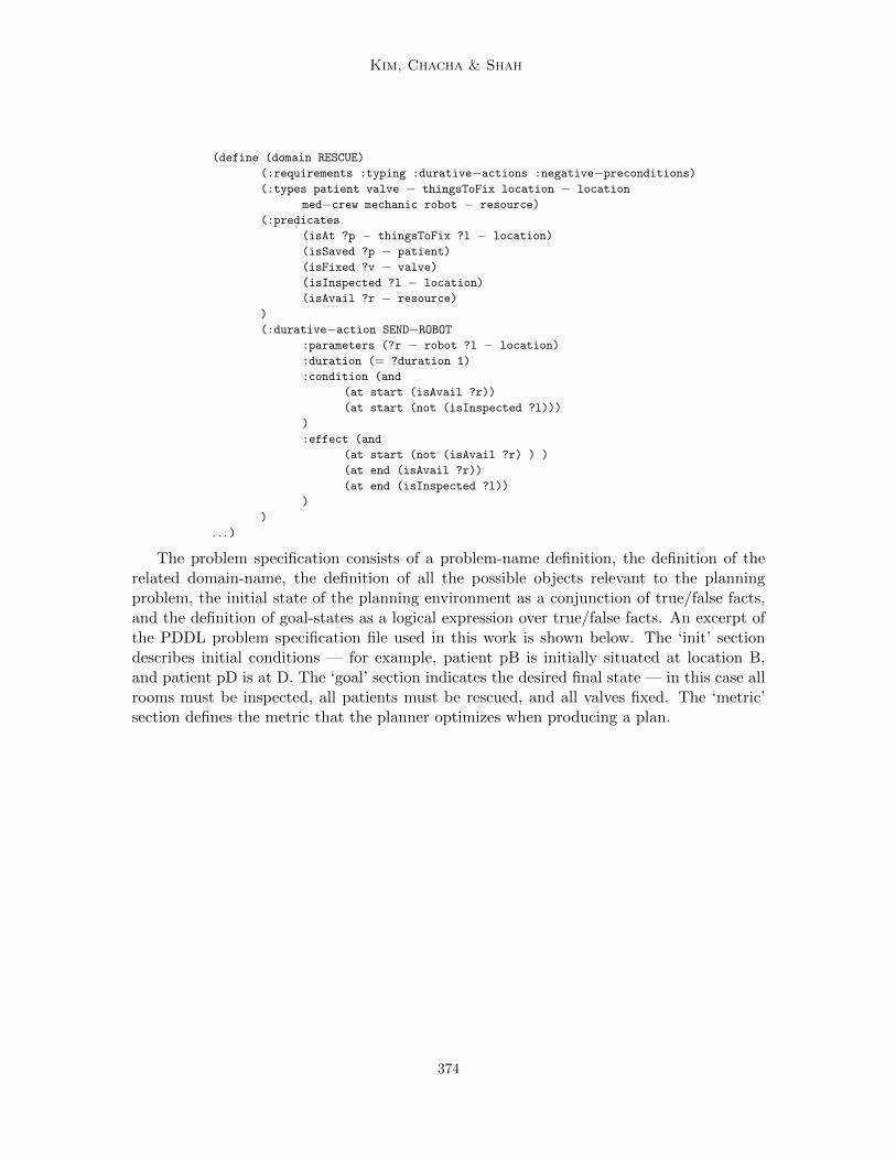
A PDDL model of a planning problem has two major components: a domain specificationand a problem specification. The domain description consists of a domain-name definition,requirements on language expressivity, definition of object types, definition of constantobjects, definition of predicates (i.e. templates for logical facts), and the definition ofpossible actions that are instantiated during execution. Actions have parameters that maybe instantiated with objects, preconditions, and conditional or unconditional effects. Anexcerpt of the PDDL domain file used in this work, called the RESCUE domain, is shownbelow. For example, the predicate isSaved encodes the logical fact of whether or not aparticular patient has been rescued, and the action SEND−ROBOT is instantiated duringexecution to send a particular robot to particular location.
373
Kim, Chacha & Shah
(define (domain RESCUE)
(:requirements :typing :durative−actions :negative−preconditions)(:types patient valve − thingsToFix location − location
med−crew mechanic robot − resource)
(:predicates
(isAt ?p − thingsToFix ?l − location)
(isSaved ?p − patient)
(isFixed ?v − valve)
(isInspected ?l − location)
(isAvail ?r − resource)
)
(:durative−action SEND−ROBOT:parameters (?r − robot ?l − location)
:duration (= ?duration 1)
:condition (and
(at start (isAvail ?r))
(at start (not (isInspected ?l)))
)
:effect (and
(at start (not (isAvail ?r) ) )
(at end (isAvail ?r))
(at end (isInspected ?l))
)
)
. . . )
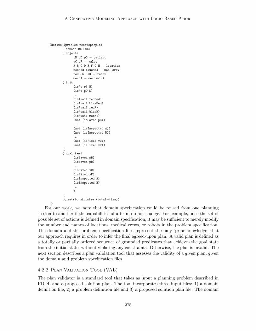
The problem specification consists of a problem-name definition, the definition of therelated domain-name, the definition of all the possible objects relevant to the planningproblem, the initial state of the planning environment as a conjunction of true/false facts,and the definition of goal-states as a logical expression over true/false facts. An excerpt ofthe PDDL problem specification file used in this work is shown below. The ‘init’ sectiondescribes initial conditions — for example, patient pB is initially situated at location B,and patient pD is at D. The ‘goal’ section indicates the desired final state — in this case allrooms must be inspected, all patients must be rescued, and all valves fixed. The ‘metric’section defines the metric that the planner optimizes when producing a plan.
374
A Generative Modeling Approach with Logic-Based Prior
(define (problem rescuepeople)
(:domain RESCUE)
(:objects
pB pD pG − patient
vC vF − valve
A B C D E F G H − location
redMed blueMed − med−crewredR blueR − robot
mech1 − mechanic)
(:init
(isAt pB B)
(isAt pD D)
. . .(isAvail redMed)
(isAvail blueMed)
(isAvail redR)
(isAvail blueR)
(isAvail mech1)
(not (isSaved pB))
. . .(not (isInspected A))
(not (isInspected B))
. . .(not (isFixed vC))
(not (isFixed vF))
)
(:goal (and
(isSaved pB)
(isSaved pD)
. . .(isFixed vC)
(isFixed vF)
(isInspected A)
(isInspected B)
. . .)
)
;(:metric minimize (total−time)))
For our work, we note that domain specification could be reused from one planningsession to another if the capabilities of a team do not change. For example, once the set ofpossible set of actions is defined in domain specification, it may be sufficient to merely modifythe number and names of locations, medical crews, or robots in the problem specification.The domain and the problem specification files represent the only ‘prior knowledge’ thatour approach requires in order to infer the final agreed-upon plan. A valid plan is defined asa totally or partially ordered sequence of grounded predicates that achieves the goal statefrom the initial state, without violating any constraints. Otherwise, the plan is invalid. Thenext section describes a plan validation tool that assesses the validity of a given plan, giventhe domain and problem specification files.
4.2.2 Plan Validation Tool (VAL)
The plan validator is a standard tool that takes as input a planning problem described inPDDL and a proposed solution plan. The tool incorporates three input files: 1) a domaindefinition file, 2) a problem definition file and 3) a proposed solution plan file. The domain
375
Kim, Chacha & Shah
definition file contains types of parameters (e.g., resources, locations), predicate definitionsand actions (which also have parameters, conditions and effects). The problem definitionfile contains information specific to the situation: For example, the number of locationsand victims, initial goal conditions and a metric to optimize. A proposed solution plan filecontains a single complete plan, described in PDDL. The output of a plan validation toolindicates whether the proposed solution plan is valid (true) or not (false).
Metrics represent ways to compute a plan quality value. For the purpose of this study,the metrics used included: 1) the minimization of total execution time for the radioactivematerial leakage scenario, and 2) the maximization of the number of incidents respondedto in the police incident response scenario. Intuitively speaking, metrics reflect the rationalbehavior of human experts. It is natural to assume that human experts would try tominimize the total time to completion of time-critical missions (such as in the radioactivematerial leakage scenario). If first responders cannot accomplish all the necessary tasks ina scenario due to limited availability of resources, they would most likely try to maximizethe number of completed tasks (such as in the police incident response scenario).
One could imagine that these input files could be reused in subsequent missions, asthe capabilities (actions) of a team may not change dramatically. However, the number ofavailable resources might vary, or there might be rules implicit in a specific situation thatare not encoded in these files (e.g., to save endangered humans first before fixing a damagedbridge). In Section 6, we demonstrate the robustness of our approach using both completeand degraded PDDL plan specifications.
The computation of a plan’s validity is generally cheaper than that of a valid plan gener-ation. This gives us a way to compute p(plan) (defined in Section 4.1) up to proportionalityin a computationally efficient manner. Leveraging this efficiency, we use Metropolis-Hastingssampling, (details described in Section 4.3.1) without calculating the partition function.
4.3 Gibbs Sampling
We use Gibbs sampling to perform inference on the generative model. There are four latentvariables to sample: plan, the collection of variables snt , ωp and β. We iterate betweensampling each latent variable, given all other variables. The PDDL validator is used whenthe plan variable is sampled.
4.3.1 Sampling Plan using Metropolis-Hastings
Unlike snt , where we can write down an analytic form to sample from the posterior, it isintractable to directly resample the plan variable, as doing so would require calculating thenumber of all possible plans, both valid and invalid. Therefore, we use a Metropolis-Hasting(MH) algorithm to sample from the plan posterior distribution within the Gibbs samplingsteps.
376

A Generative Modeling Approach with Logic-Based Prior
The posterior of plan can be represented as the product of the prior and likelihood, asfollows:
p(plan|s, p) ∝ p(plan)p(s, p|plan)
= p(plan)T∏t=1
N∏n=1
p(snt , pnt |plan)
= p(plan)T∏t=1
N∏n=1
p(snt |plan)p(pnt |plan, snt ) (7)
The MH sampling algorithm is widely used to sample from a distribution when directsampling is difficult. This algorithm allows us to sample from posterior distribution ac-cording to the user-specified proposal distribution without having to calculate the partitionfunction. The typical MH algorithm defines a proposal distribution, Q(x′|xt), which sam-ples a new point (i.e., x′: a value of the plan variable in our case) given the current pointxt. The new point can be achieved by randomly selecting one of several possible moves,as defined below. The proposed point is then accepted or rejected, with a probability ofmin(1, acceptance ratio).
Unlike simple cases, where a Gaussian distribution can be used as a proposal distribution,our distribution needs to be defined over the plan space. Recall that plan is represented asan ordered tuple of sets of predicates. In this work, the new point (i.e., a candidate plan)is generated by performing one of the following moves on the current plan:
• Move to next: Randomly select a predicate that is in the current plan, and move itto the next timestamp. If it is in the last timestamp in the plan, move it to the firsttimestamp.
• Move to previous: Randomly select a predicate that is in the current plan, and moveit to the previous timestamp. If it is in the first timestamp in the plan, move it to thelast timestamp.
• Add a predicate to plan: Randomly select a predicate that is not in the current plan,and randomly choose one timestamp in the current plan. Add the predicate to thechosen timestamp.
• Remove a predicate from plan: Randomly select and remove a predicate that is in thecurrent plan.
These moves are sufficient to allow for movement from one arbitrary plan to another.The intuition behind designing this proposal distribution is described in Section 7.5.
Note that the proposal distribution, as it is, is not symmetrical — Q(x′|xt) 6= Q(xt|x′).We need to compensate for that according to the following,
p∗(x′)Q(x′|xt) = p∗(x)Q(xt|x′), (8)
where p∗ is the target distribution. This can be done simply by counting the number ofmoves possible from x′ to get to x, and from x′ to x, and weighing the acceptance ratio such
377

Kim, Chacha & Shah
that Equation 8 is true. This is often referred to as Hastings correction, which is performedto ensure that the proposal distribution does not favor some states over others.
Next, the ratios of the proposal distribution at the current and proposed points arecalculated. When plan is valid, p(plan) is proportional to eα, and when plan is invalid,it is proportional to 1, as described in Equation 1. Plan validity is calculated using theplan validation tool. The remaining term, p(snt |plan)p(pnt |plan, snt ), is calculated usingEquations 2 and 6.
Then, the proposed plan is accepted with the following probability:
min(
1, p∗(plan=x′|s,p)p∗(plan=xt|s,p)
), where p∗ is a function proportional to the posterior distribution.
Although we chose to incorporate MH, it is not the only usable sampling method. Anyother method that does not require calculation of the normalization constant (e.g., rejectionsampling or slice sampling) could also be used. However, for some methods, sampling fromthe ordered tuple of sets of grounded predicates can be slow and complicated, as pointedout by Neal (2003).
4.3.2 Sampling Hyper-Parameters β and ωp with Slice Sampling
We use slice sampling to sample both β and ωp. This method is simple to implement andworks well with scalar variables. Distribution choices are made based on the valid valueeach can take. β can take any value, preferably with one mode, while ωp can only take avalue between [0, 1]. MH sampling may also work; however, this method could be overlycomplicated for a simple scalar value. We chose the stepping out procedure, as describedby Neal et al (Neal, 2003).
4.3.3 Sampling snt
Fortunately, an analytic expression exists for the posterior of snt :
p(st|plan, pt, s′t) ∝ p(st|plan)p(pt, s′t|plan, st)
= p(st|plan)p(pt|plan, st)p(s′t|st)
= p(s′t|st)N∏n=1
p(snt |plan)p(pnt |plan, snt )
Note that this analytic expression can be expensive to evaluate if the number of possiblevalues of snt is large. In that case, one can marginalize snt , as the variable we truly careabout is the plan variable.
5. Experimentation
In this section, we explain the web-based collaboration tool that is used in our experimentand two fictional rescue scenarios given to human subjects in the experiment.
5.1 Web-Based Tool Design
Disaster response teams are increasingly using web-based tools to coordinate missions andshare situational awareness. One of the tools currently used by first responders is the Next
378
A Generative Modeling Approach with Logic-Based Prior
Generation Incident Command System (NICS) (Di Ciaccio et al., 2011). This integratedsensing and command-and-control system enables the distribution of large-scale coordina-tion across multiple jurisdictions and agencies. It provides video and audio conferencingcapabilities, drawing tools and a chat window, and allows for the sharing of maps and re-source information. Overall, the NICS enables the collection and exchange of informationcritical to mission planning.
We designed a web-based collaboration tool modeled after this system, with a modifi-cation that requires the team to communicate solely via text chat. This tool was developedusing Django (Holovaty & Kaplan-Moss, 2009), a free and open-source Web applicationframework written in Python. Django is designed to ease working with heavy-duty data,and provides a Python API to enable rapid prototyping and testing. Incoming data can beeasily maintained through a user-friendly administrative interface. Although it is a simpli-fied version of the NICS, it provides the essence of the emerging technology for large-scaledisaster coordination (Figure 1).
5.2 Scenarios
Human subjects were given one of two fictional rescue scenarios and asked to formulate aplan by collaborating with their partners. We collected human team planning data fromthe resulting conversations, and used this data to validate our algorithm. The first sce-nario involves a radioactive material leakage accident in a building with multiple rooms,where all tasks (described below) were assumed to take one unit of time. We added com-plexity to the scenario by announcing a new piece of information halfway through theplanning conversation, requiring the team to change their plan. The second scenario alsoincluded time-durative actions (e.g., action A can only take place if action B is takingplace). These scenarios are inspired by those described in emergency response team train-ing manuals (FEMA, 2014), and are designed to be completed in the reasonable time forour experiments.
5.2.1 First Scenario: Radioactive Material Leakage
This disaster scenario involves the leakage of radioactive material on a floor consisting ofeight rooms. Each room contains either a patient requiring in-person assessment or a valvethat must be repaired (Figure 4).
Goal State: All patients are assessed in-person by a medical crew. All valves are fixedby a mechanic. All rooms are inspected by a robot.
Constraints: There are two medical crews, red and blue (discrete resource constraint),one human mechanic (discrete resource constraint) and two robots, red and blue (discreteresource constraint). For safety purposes, a robot must inspect the radioactivity of a roombefore human crews can be sent inside (sequence constraint).
Assumption: All tasks (e.g. inspecting a room, fixing a valve) take the same amount oftime (one unit), and there are no hard temporal constraints. This assumption was made toconduct the initial proof-of-concept experimentation described in this paper, and is relaxedin the scenario described in Section 5.2.2.
379

Kim, Chacha & Shah
Figure 3: Radioactive material leakage scenario
Announcement: During the planning session, the team receives a situation update thatthe red robot is now out of order, requiring the team to modify their previously discussedplan to only use one robot for deployment. The announcement triggers automatically oncethe team has exchanged 20 utterances. The purpose of this announcement is to increasetask complexity for the team, to have at least two competing plans and to increase the levelof noise in the conversation.
This scenario produces a large number of possible plans (more than 1012), many of whichare valid for achieving the goals without violating the constraints.
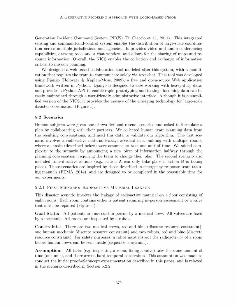
5.2.2 Second Scenario: Police Incidents Response
The second scenario involves a team of police officers and firefighters responding to a seriesof incidents occurring in different time frames. This scenario includes more complicatedtime-durative actions than the first, as well as interdependency of tasks that has to betaken into account when planning. The current time is given as 8 p.m. Two fires havestarted at this time: one at a college dorm and another at a theater building, as shownin Figure 4. Also, three street corners, indicated as crime hot-spots (places predicted toexperience serious crimes, based on prior data), become active between 8:30 p.m. and 9 p.m.There is also a report of a street robbery taking place at 8 p.m. No injury has occurred;however, a police officer must speak with the victim to file an incident report.
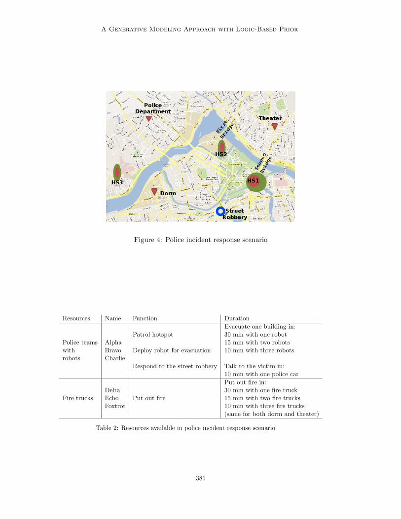
Goal State: Respond to as many incidents as possible given the resources listed in Table2.
Constraints:• Putting out a fire requires one fire truck and one police car equipped with a robot.• A police car must stay with the robot until an evacuation is over.• Only a robot can perform an evacuation.• Each robot can only be used once.• Successfully responding to a fire requires both evacuating the building and putting
out the fire. Both actions can happen simultaneously.
380
A Generative Modeling Approach with Logic-Based Prior
Figure 4: Police incident response scenario
Resources Name Function Duration
Evacuate one building in:Patrol hotspot 30 min with one robot
Police teams Alpha 15 min with two robotswith Bravo Deploy robot for evacuation 10 min with three robotsrobots Charlie
Respond to the street robbery Talk to the victim in:10 min with one police car
Put out fire in:Delta 30 min with one fire truck
Fire trucks Echo Put out fire 15 min with two fire trucksFoxtrot 10 min with three fire trucks
(same for both dorm and theater)
Table 2: Resources available in police incident response scenario
381

Kim, Chacha & Shah
• Responding to a hot-spot patrol requires one police car to be located at the site for aspecified amount of time.• Only one police car is necessary to respond to the street robbery.
Assumption and Announcement: If no information about traffic is provided, the traveltime from place to place is assumed to be negligible. During the planning session, the teamreceives the following announcement: “The traffic officer just contacted us, and said theFirst and Second bridges will experience heavy traffic at 8:15 pm. It will take at least 20minutes for any car to get across a bridge. The travel time from the theater to any hot-spotis about 20 minutes without using the bridges.” Once this announcement is made, the teammust account for the traffic in their plan.
6. Evaluation
In this section, we evaluate the performance of our plan inference algorithm through initialproof-of-concept human subject experimentation, and show we are able to infer a humanteam’s final plan with 86% accuracy on average, where “accuracy” is defined as a compositemeasure of task allocation and plan sequence accuracy measures. We also describe a robotdemonstration in which two people plan and execute a first-response collaborative task witha PR2 robot.
6.1 Human Team Planning Data
As indicated previously, we designed a web-based collaboration tool modeled after the NICSsystem (Di Ciaccio et al., 2011) used by first-response teams, but with a modification thatrequires the team to communicate solely via text chat. For the radioactive material leakagescenario, before announcement, 13 teams of two (a total of 26 participants) were recruitedthrough Amazon Mechanical Turk and from the greater Boston area. Recruitment wasrestricted to those located in the US to increase the probability that participants werefluent in English. For the radioactive material leakage scenario, after announcement, 21teams of two (a total of 42 participants) were recruited through Amazon Mechanical Turkand from the greater Boston area. For the police incident response scenario, 14 teams oftwo (total 28 participants) were recruited from the greater Boston area. Participants werenot required to have prior experience or expertise in emergency or disaster planning, andwe note that there may be structural differences in the dialog of expert and novice planners.We leave this topic for future investigation.
Each team received one of the two fictional rescue scenarios described in Section 5.2, andwas asked to collaboratively plan a rescue mission. Upon completion of the planning session,each participant was asked to summarize the final agreed-upon plan in the structured formdescribed previously. An independent analyst reviewed the planning sessions to resolvediscrepancies between the two members’ descriptions when necessary. The first and secondauthors, as well as two independent analysts, performed utterance tagging, with each teamplanning session tagged and reviewed by two of these four analysts. On average, 36% ofpredicates mentioned per data set did not end up in the final plan.
382
A Generative Modeling Approach with Logic-Based Prior
6.2 Algorithm Implementation
The algorithm was implemented in Python, and the VAL PDDL 2.1 plan validator (Howeyet al., 2004) was used. We performed 2,000 Gibbs sampling steps on the data from eachplanning session. The initial plan value was set to two to five moves (from MH proposaldistribution) away from the true plan. The initial value for s variable was randomly set toany timestamp in the initial plan value.
Within one Gibbs sampling step, we performed 30 steps of the Metropolis-Hastings(MH) algorithm to sample the plan. Every 20 samples were selected to measure accuracy(median), after a burn-in period of 200 samples.Results We assessed the quality of the final plan produced by our algorithm in terms ofthe accuracy of task allocation among agents (e.g. which medic travels to which room) andthe accuracy of the plan sequence.
Two metrics for task allocation accuracy were evaluated: 1) The percent of inferred planpredicates appearing in the team’s final plan [% Inferred], and 2) the percent noise rejectionof extraneous predicates that were discussed but do not appear in the team’s final plan [%Noise Rej].
We evaluated the accuracy of the plan sequence as follows: A pair of predicates iscorrectly ordered if it is consistent with the relative ordering in the true final plan. We mea-sured the percent accuracy of sequencing [% Seq] by # correctly ordered pairs of correct predicates
total # of pairs of correct predicates .Only correctly estimated predicates were compared, as there is no ground truth relation forpredicates not included in the true final plan. We used this relative sequencing measurebecause it does not compound sequence errors, as an absolute difference measure would(e.g. where an error in the ordering of one predicate early in the plan shifts the position ofall subsequent predicates).
Overall “composite” plan accuracy was computed as the arithmetic mean of the taskallocation and plan sequence accuracy measures. This metric summarizes the two relevantaccuracy measures so as to provide a single metric for comparison between conditions. Weevaluated our algorithm under four conditions: 1) perfect PDDL files, 2) PDDL problem filewith missing goals/constants (e.g. delete available agents), 3) PDDL domain file missinga constraint (e.g. delete precondition), and 4) using an uninformative prior over possibleplans.
The purpose of the second condition, PDDL problem file with missing goals/constants,was to test the robustness of our approach to incomplete problem information. This PDDLproblem specifiction was intentionally designed to omit information regarding one patient(pG) and one robot (blueR). It also omitted the following facts about the initial state:that pG was located at G, the blueR was available to perform inspections, and patient pGpatient was not yet rescued. The goal state omitted that pG patient was to be rescued.This condition represented a significant degradation of the problem definition file, since theoriginal planning problem involved only three patients and two robots.
The purpose of the third condition, PDDL domain file with a missing constant, was totest the robustness of our approach to missing constraints (or rules for successful execution).It is potentially easy for a person to miss specifying a rule that is often implicitly assumed.The third condition omitted the following constraint from the domain file: all the rooms areto be inspected prior to sending any medical crews. This condition represented a significant
383
Kim, Chacha & Shah
degradation of the domain file, since this constraint affected any action involving one of themedical crew teams.
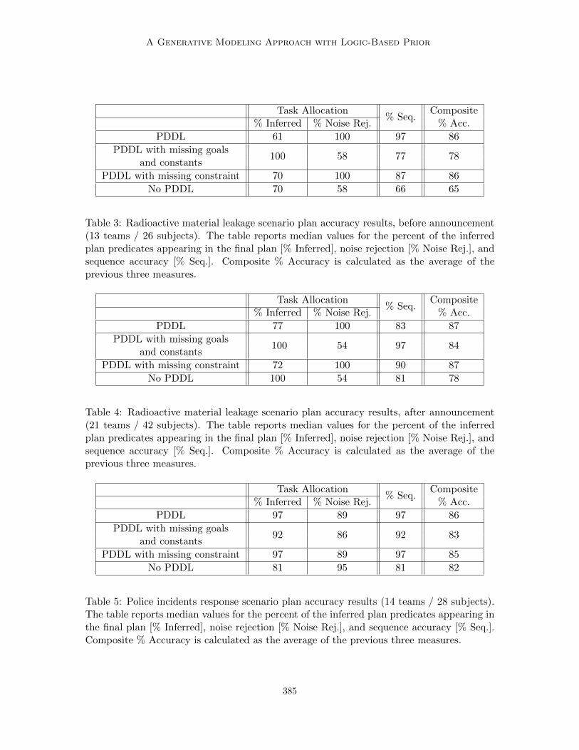
Results shown in Tables 3-5 are produced by sampling plan and s variables and fixingβ = 5 and ωp = 0.8. The tables report median values for the percent of the inferredplan predicates appearing in the final plan [% Inferred], noise rejection [% Noise Rej.], andsequence accuracy [% Seq.]. We show that our algorithm infers final plans with greater than86% composite accuracy on average. We also show that our approach is relatively robust todegraded PDDL specifications (i.e., PDDL with missing goals, constants and constraints).Further discussion of sampling hyper-parameters is found in Section 7.2.
6.3 Concept-of-Operations Robot Demonstration
We illustrate the use of our plan inference algorithm through a robot demonstration inwhich two people plan and execute a first-response collaborative task with a PR2 robot.The participants plan an impending deployment using the web-based collaborative tool wedeveloped. Once the planning session is complete, the dialogue is tagged manually. Theplan inferred from this data is confirmed with the human planners and provided to therobot for execution. The registration of predicates to robot actions, and room names tomap locations, is performed offline in advance. While the first responders are on their wayto the accident scene, the PR2 autonomously navigates to each room, performing onlinelocalization, path planning and obstacle avoidance. The robot informs the rest of the teamas it inspects each room and confirms it is safe for human team members to enter. Videoof this demo can be found here: http://tiny.cc/uxhcrw.
7. Discussion
In this section we discuss the results and trends in Tables 3-5. We then discuss how sam-pling hyper-parameters improves inference accuracy, and provide an interpretation of in-ferred hyper-parameter values and how they relate to data characteristics. We also provideadditional support for the use of PDDL by analyzing multiple Gibbs sampling runs. Our ra-tionale behind the i.i.d assumption on utterances made in the generative model is explained,and we show how a simple extension to our model can relax this assumption. Finally, weprovide our rationale for designing the proposal distribution for the sampling algorithm.
7.1 Results
The average accuracy of the inferred final plan improved across all three scenarios withthe use of perfect PDDL as compared to an uninformative prior over possible plans. Thesequence accuracy also consistency improved with the use PDDL, regardless of noise levelor the type of PDDL degradation. The three scenarios exhibited different levels of “noise,”defined as the percentage of utterances that did not end up in the finally agreed uponplan. The police incidents response scenario produced substantially higher noise (53%),as compared to the radioactive material leaking scenario before announcement (38%) andafter announcement (17%). This is possibly because the police incidents scenario includeddurative-actions, whereas the others did not. Interestingly, perfect PDDL produced more
384
A Generative Modeling Approach with Logic-Based Prior
Task Allocation% Seq.
Composite% Inferred % Noise Rej. % Acc.
PDDL 61 100 97 86
PDDL with missing goals100 58 77 78
and constants
PDDL with missing constraint 70 100 87 86
No PDDL 70 58 66 65
Table 3: Radioactive material leakage scenario plan accuracy results, before announcement(13 teams / 26 subjects). The table reports median values for the percent of the inferredplan predicates appearing in the final plan [% Inferred], noise rejection [% Noise Rej.], andsequence accuracy [% Seq.]. Composite % Accuracy is calculated as the average of theprevious three measures.
Task Allocation% Seq.
Composite% Inferred % Noise Rej. % Acc.
PDDL 77 100 83 87
PDDL with missing goals100 54 97 84
and constants
PDDL with missing constraint 72 100 90 87
No PDDL 100 54 81 78
Table 4: Radioactive material leakage scenario plan accuracy results, after announcement(21 teams / 42 subjects). The table reports median values for the percent of the inferredplan predicates appearing in the final plan [% Inferred], noise rejection [% Noise Rej.], andsequence accuracy [% Seq.]. Composite % Accuracy is calculated as the average of theprevious three measures.
Task Allocation% Seq.
Composite% Inferred % Noise Rej. % Acc.
PDDL 97 89 97 86
PDDL with missing goals92 86 92 83
and constants
PDDL with missing constraint 97 89 97 85
No PDDL 81 95 81 82
Table 5: Police incidents response scenario plan accuracy results (14 teams / 28 subjects).The table reports median values for the percent of the inferred plan predicates appearing inthe final plan [% Inferred], noise rejection [% Noise Rej.], and sequence accuracy [% Seq.].Composite % Accuracy is calculated as the average of the previous three measures.
385
Kim, Chacha & Shah
substantial improvements in sequence accuracy when noise level was higher, in the radioac-tive material leaking scenario before announcement, and in police incidents scenario.
Accuracy in task allocation, on the other hand, did differ depending on the noise leveland the type of PDDL degradation. The noise rejection ratio was the same or better withPDDL or PDDL with a missing constraint, as compared to an uninformative prior, forscenarios with less noise (e.g. the radioactive material leaking scenarios before and afterannouncement). However, PDDL did not provide benefit to the noise rejection ratio for thepolice incidents scenario where the noise level was more than 50%. However, in this casePDDL did provide improvements in inferred task allocation.
7.2 Sampling Hyper-Parameters
This section discusses the results of hyper-parameter sampling. First, we show that eachdata point (i.e., each team’s conversation) converges to different hyper-parameter values,then show that those values capture the characteristics of each data point. Second, we showhow learning different sets of hyper-parameters improves different measures of accuracy,and describe how this is consistent with our interpretation of the hyper-parameters in ourmodel.
-10%
0%
10%
20%
30%
40%
50%
0% 0%
11%
42%46%
13%
0% 0%
10%
42%46%
5%
PDDLPDDL with missing goals and constantsPDDL with missing constraintNo PDDL
Radioactive before Radioactive after Police
% im
prov
ed a
ccur
acy
(a) Improvements in noise rejection when samplingωp
-10%
-5%
0%
5%
10%
15%
20%
25%
30%
-4%
17%
3%
17%
-8%
5%
12%
-7% 0%
26%
12%
18%
PDDLPDDL with missing goals and constantsPDDL with missing constraintNo PDDL
Radioactive before Radioactive after Police
% im
prov
ed a
ccur
acy
(b) Improvements in sequence accuracy when sam-pling β
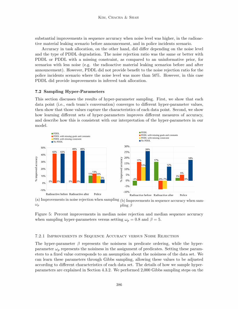
Figure 5: Percent improvements in median noise rejection and median sequence accuracywhen sampling hyper-parameters versus setting ωp = 0.8 and β = 5.
7.2.1 Improvements in Sequence Accuracy versus Noise Rejection
The hyper-parameter β represents the noisiness in predicate ordering, while the hyper-parameter ωp represents the noisiness in the assignment of predicates. Setting these param-eters to a fixed value corresponds to an assumption about the noisiness of the data set. Wecan learn these parameters through Gibbs sampling, allowing these values to be adjustedaccording to different characteristics of each data set. The details of how we sample hyper-parameters are explained in Section 4.3.2. We performed 2,000 Gibbs sampling steps on the
386

A Generative Modeling Approach with Logic-Based Prior
data from each planning session. The initial values of ωp and β were sampled from theirprior, where the parameters were set to the values described in Section 4.1.
We found that when we learned ωp (with β = 5), the noise rejection rate improvedcompared with when we fixed ωp = 0.8. In the radioactive material leakage scenario, bothbefore and after the mid-scenario announcement, the noise rejection ratio was improved byas much as 41% and 45%, respectively; in the police incident response scenario, we observedup to a 13% improvement (Figure 5a). Note that in all cases the median noise rejectionratio was maintained or improved with the sampling of ωp.
Similarly, when we learned β (with ωp = 0.8), sequence accuracies generally improved. Inthe radioactive material leakage scenario, before and after the announcement, the sequenceaccuracy improved by up to 26% and 16%, respectively; in the police incident responsescenario, we observed up to an 18% improvement (Figure 5b). Note that three cases didsee a degradation in accuracy of up to 4-8%. However in nine out of the twelve cases thesequence accuracy was maintained or improved with the sampling of β.
Interestingly, most of the samples achieved the highest overall composite accuracy whenonly plan and s were learned, and the hyper-parameters were fixed. In particular, weobserved an average 5% (± 3%) decrease in composite accuracy when sampling all fourvariables together. One of the possible explanations for this finding is that, due to thelimited amount of data, Gibbs sampling may require many more iterations to converge allthe variables. This result suggests that one may choose the set of hyper-parameters to learnbased on which measure of accuracy is more important to the user.
7.2.2 Interpretation of Inferred Values of Hyper-Parameters
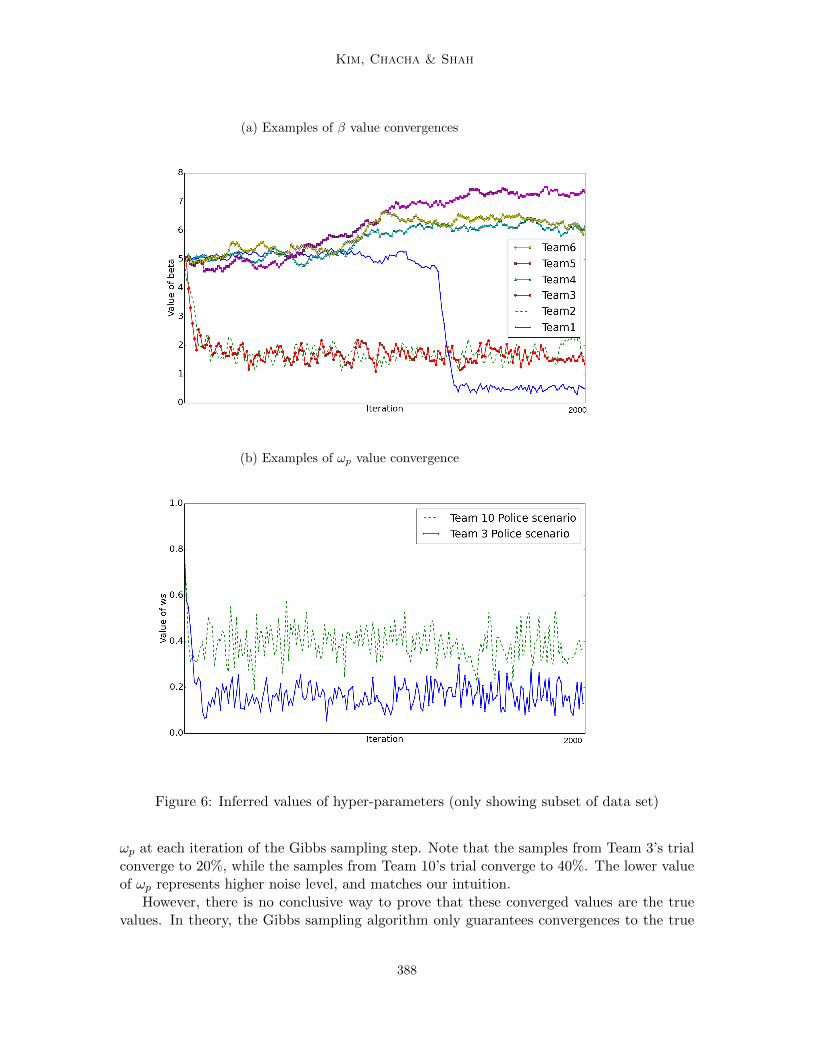
As described in Section 4.1, the ωp parameter models the level of noise in predicates withinthe data. In other words, the ωp parameter is designed to model how many suggestions theteam makes during the conversation that are subsequently included in the final plan. If thenoise level is high, a lower-valued ωp will represent the characteristics of the conversationwell, which may allow for better performance. (However, if the noise level is too high, theinference may still fail.)
To compare the learned value of ωp with the characteristics of the conversation, we needa way to calculate how noisy the conversation is. The following is one way to manuallyestimate the value of ωp: First, count the utterances that contain any predicates. Then,count the utterances that contain predicates included in the final plan. The ratio betweenthese two numbers can be interpreted as noisiness in the predicates; the lower the number,the more the team talked about many possible plans.
We performed this manual calculation for two teams’ trials — Team 3 and 10 — tocompare their values to the learned values. In Team 3’s trial, only 19.4% of the suggestionsmade during the conversation were included in the final plan (i.e., almost 80% of suggestionswere not relevant to the final plan). On the other hand, 68% of suggestions made in Team10’s trial were included in the final plan. Using this interpretation, Team 3’s trial is morethan twice as noisy as Team 10’s trial.
The converged value of ωp is lower in Team 3’s trial than in Team 10’s trial, reflectingthe characteristics of each data set. Figure 6b shows the converged value of ωp for eachteam’s trial (sub-sampled, and for a subset of the dataset). The figure presents values of
387
Kim, Chacha & Shah
(a) Examples of β value convergences
(b) Examples of ωp value convergence
Figure 6: Inferred values of hyper-parameters (only showing subset of data set)
ωp at each iteration of the Gibbs sampling step. Note that the samples from Team 3’s trialconverge to 20%, while the samples from Team 10’s trial converge to 40%. The lower valueof ωp represents higher noise level, and matches our intuition.
However, there is no conclusive way to prove that these converged values are the truevalues. In theory, the Gibbs sampling algorithm only guarantees convergences to the true
388
A Generative Modeling Approach with Logic-Based Prior
value with an infinite number of iterations. Therefore, we cannot prove that the convergedωp variables shown in Figure 6 are the true values. In practice, a trace plot, such as thatin Figure 6, is drawn in order to demonstrate convergence to a local optimum. The factthat the values appear to plateau after a burn-in period provides support of convergenceto a local optimum point. Investigation of this potentially local optimum point suggeststhat the ωp value for each data point can be different, and that we can observe somerelationship between the ωp value and the characteristics of the data set. In addition, themanual calculation of ‘noisiness’ is only one way of interpreting the ‘noisiness’ of the dataset. Therefore, this analysis should be considered as one possible way to gain insight intothe learned values; not a rigorous proof of the relation between the learned value of thehyper-parameter and the characteristics of the data.
7.3 The Benefit of PDDL
This section provides additional evidence of the benefit of using PDDL by analyzing multipleruns using the same data and sampling algorithm. As explained in Section 4.3, Gibbssampling is an approximate inference algorithm that can produce different results on eachrun.
In this section we evaluate runs over a wide range of different settings to show that thebenefit of PDDL applies not just to a particular setting of parameters, but also to differentsettings. We analyzed three cases across a range of parameters: 1) learning both plan ands, 2) learning plan, s and ωp and 3) learning plan, s and β. In the first case, we changed thevalue of α to range from 3 to 1,000, ωp from 0.3 to 0.8, and β from 1 to 100. In the secondcase, in addition to α and β parameters, we varied the parameters for the prior distributionof ωp — kωp and θωp ; both ranging from 2 to 70. In the third case, in addition to α andωp parameters, we varied the parameters for the prior distribution of β — kβ and θβ; bothranging from 0.1 to 50. Values from the all ranges were selected randomly to produce atotal of 613 runs.
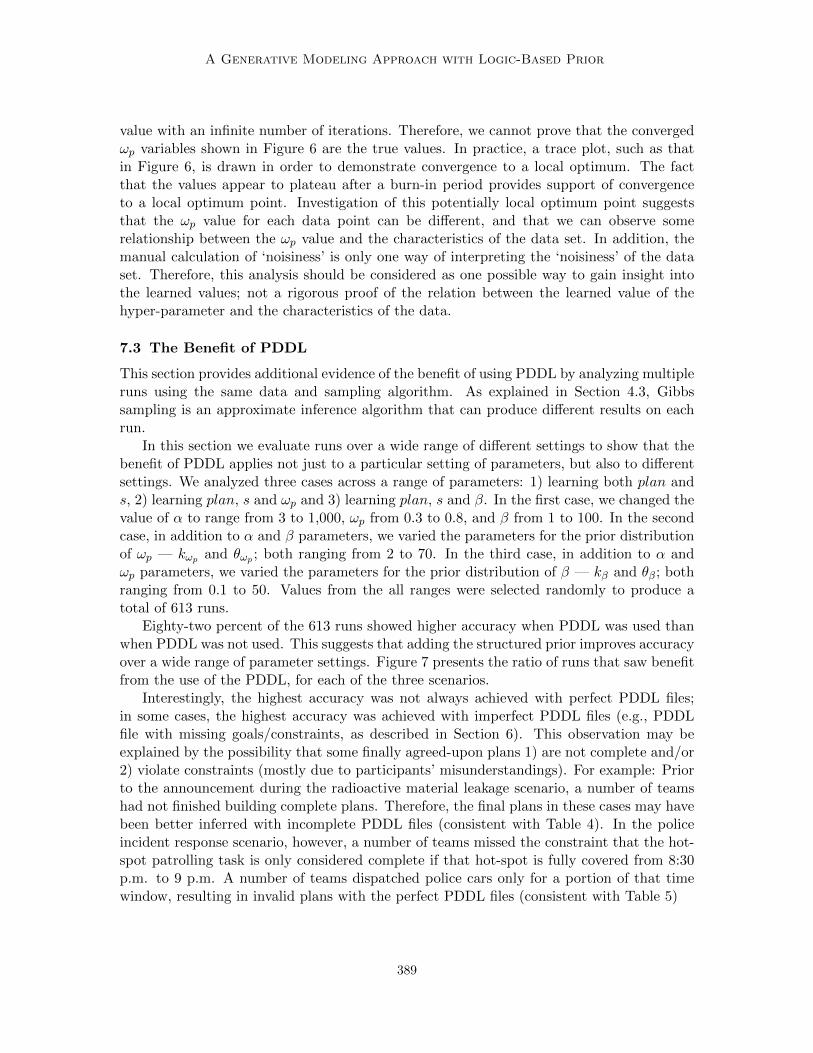
Eighty-two percent of the 613 runs showed higher accuracy when PDDL was used thanwhen PDDL was not used. This suggests that adding the structured prior improves accuracyover a wide range of parameter settings. Figure 7 presents the ratio of runs that saw benefitfrom the use of the PDDL, for each of the three scenarios.
Interestingly, the highest accuracy was not always achieved with perfect PDDL files;in some cases, the highest accuracy was achieved with imperfect PDDL files (e.g., PDDLfile with missing goals/constraints, as described in Section 6). This observation may beexplained by the possibility that some finally agreed-upon plans 1) are not complete and/or2) violate constraints (mostly due to participants’ misunderstandings). For example: Priorto the announcement during the radioactive material leakage scenario, a number of teamshad not finished building complete plans. Therefore, the final plans in these cases may havebeen better inferred with incomplete PDDL files (consistent with Table 4). In the policeincident response scenario, however, a number of teams missed the constraint that the hot-spot patrolling task is only considered complete if that hot-spot is fully covered from 8:30p.m. to 9 p.m. A number of teams dispatched police cars only for a portion of that timewindow, resulting in invalid plans with the perfect PDDL files (consistent with Table 5)
389
Kim, Chacha & Shah
Radioactive before Radioactive after Police0
0.1
0.2
0.3
0.4
0.5
0.6
0.7
0.8
0.9
1
Rat
io o
f run
s us
ing
PD
DL
tha
t im
pro
ved
com
posi
te a
ccur
acy
173/216198/230
134/167
Figure 7: Ratio of runs that show the benefit of using PDDL
The improvements achieved by adding the structure to the prior using PDDL suggestthat the structural information is beneficial to our inference problem. It would be interestingto systematically investigate the smallest set of structural information that achieves accuracyimprovements, given a fixed computation budget, in future work.
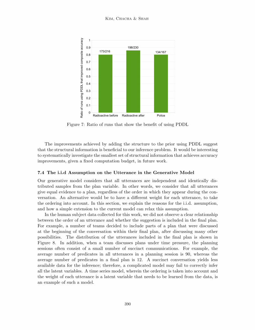
7.4 The i.i.d Assumption on the Utterance in the Generative Model
Our generative model considers that all utterances are independent and identically dis-tributed samples from the plan variable. In other words, we consider that all utterancesgive equal evidence to a plan, regardless of the order in which they appear during the con-versation. An alternative would be to have a different weight for each utterance, to takethe ordering into account. In this section, we explain the reasons for the i.i.d. assumption,and how a simple extension to the current model can relax this assumption.
In the human subject data collected for this work, we did not observe a clear relationshipbetween the order of an utterance and whether the suggestion is included in the final plan.For example, a number of teams decided to include parts of a plan that were discussedat the beginning of the conversation within their final plan, after discussing many otherpossibilities. The distribution of the utterances included in the final plan is shown inFigure 8. In addition, when a team discusses plans under time pressure, the planningsessions often consist of a small number of succinct communications. For example, theaverage number of predicates in all utterances in a planning session is 90, whereas theaverage number of predicates in a final plan is 12. A succinct conversation yields lessavailable data for the inference; therefore, a complicated model may fail to correctly inferall the latent variables. A time series model, wherein the ordering is taken into account andthe weight of each utterance is a latent variable that needs to be learned from the data, isan example of such a model.
390
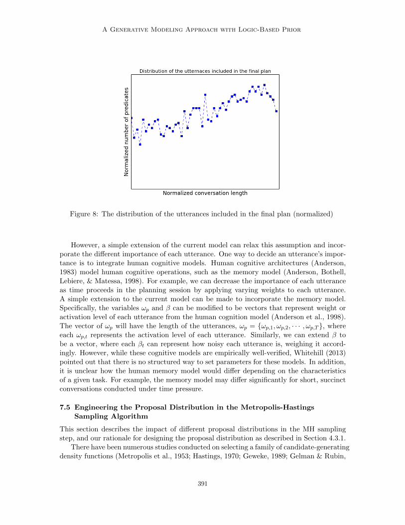
A Generative Modeling Approach with Logic-Based Prior
Figure 8: The distribution of the utterances included in the final plan (normalized)
However, a simple extension of the current model can relax this assumption and incor-porate the different importance of each utterance. One way to decide an utterance’s impor-tance is to integrate human cognitive models. Human cognitive architectures (Anderson,1983) model human cognitive operations, such as the memory model (Anderson, Bothell,Lebiere, & Matessa, 1998). For example, we can decrease the importance of each utteranceas time proceeds in the planning session by applying varying weights to each utterance.A simple extension to the current model can be made to incorporate the memory model.Specifically, the variables ωp and β can be modified to be vectors that represent weight oractivation level of each utterance from the human cognition model (Anderson et al., 1998).The vector of ωp will have the length of the utterances, ωp = {ωp,1, ωp,2, · · · , ωp,T }, whereeach ωp,t represents the activation level of each utterance. Similarly, we can extend β tobe a vector, where each βt can represent how noisy each utterance is, weighing it accord-ingly. However, while these cognitive models are empirically well-verified, Whitehill (2013)pointed out that there is no structured way to set parameters for these models. In addition,it is unclear how the human memory model would differ depending on the characteristicsof a given task. For example, the memory model may differ significantly for short, succinctconversations conducted under time pressure.
7.5 Engineering the Proposal Distribution in the Metropolis-HastingsSampling Algorithm
This section describes the impact of different proposal distributions in the MH samplingstep, and our rationale for designing the proposal distribution as described in Section 4.3.1.
There have been numerous studies conducted on selecting a family of candidate-generatingdensity functions (Metropolis et al., 1953; Hastings, 1970; Geweke, 1989; Gelman & Rubin,
391
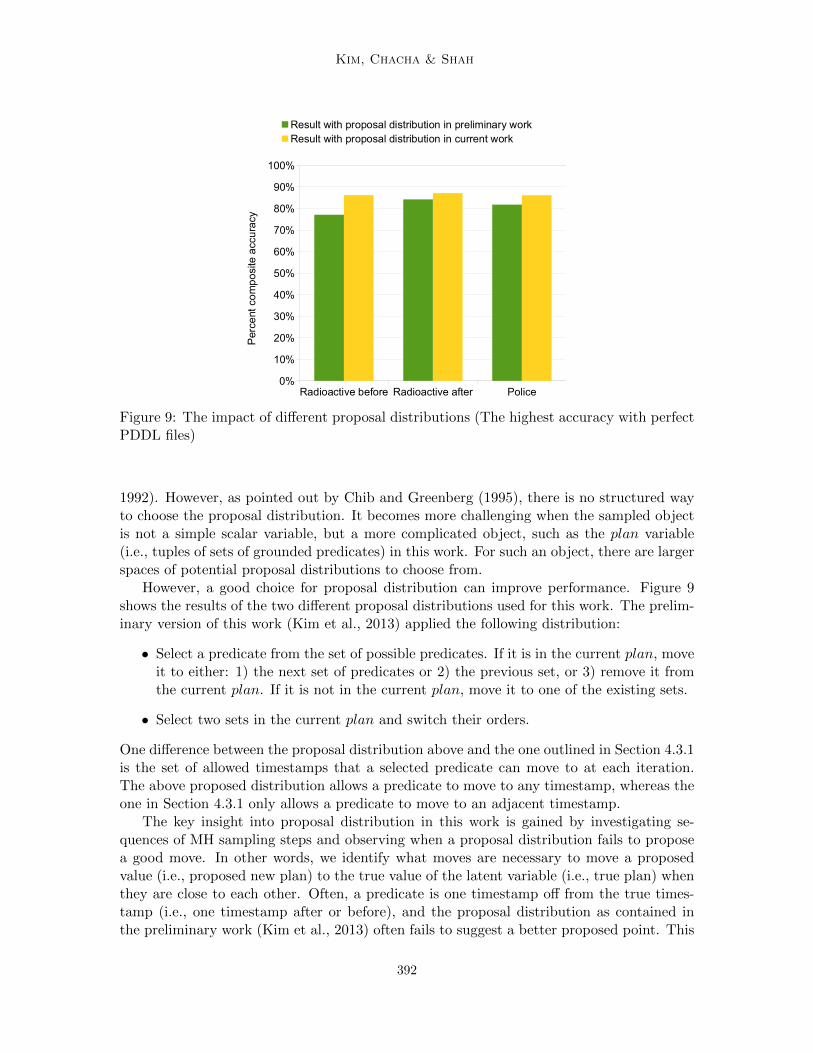
Kim, Chacha & Shah
Radioactive before Radioactive after Police0%
10%
20%
30%
40%
50%
60%
70%
80%
90%
100%
Result with proposal distribution in preliminary workResult with proposal distribution in current work
Per
cent
co
mp
osi
te a
ccu
racy
Figure 9: The impact of different proposal distributions (The highest accuracy with perfectPDDL files)
1992). However, as pointed out by Chib and Greenberg (1995), there is no structured wayto choose the proposal distribution. It becomes more challenging when the sampled objectis not a simple scalar variable, but a more complicated object, such as the plan variable(i.e., tuples of sets of grounded predicates) in this work. For such an object, there are largerspaces of potential proposal distributions to choose from.
However, a good choice for proposal distribution can improve performance. Figure 9shows the results of the two different proposal distributions used for this work. The prelim-inary version of this work (Kim et al., 2013) applied the following distribution:
• Select a predicate from the set of possible predicates. If it is in the current plan, moveit to either: 1) the next set of predicates or 2) the previous set, or 3) remove it fromthe current plan. If it is not in the current plan, move it to one of the existing sets.
• Select two sets in the current plan and switch their orders.
One difference between the proposal distribution above and the one outlined in Section 4.3.1is the set of allowed timestamps that a selected predicate can move to at each iteration.The above proposed distribution allows a predicate to move to any timestamp, whereas theone in Section 4.3.1 only allows a predicate to move to an adjacent timestamp.
The key insight into proposal distribution in this work is gained by investigating se-quences of MH sampling steps and observing when a proposal distribution fails to proposea good move. In other words, we identify what moves are necessary to move a proposedvalue (i.e., proposed new plan) to the true value of the latent variable (i.e., true plan) whenthey are close to each other. Often, a predicate is one timestamp off from the true times-tamp (i.e., one timestamp after or before), and the proposal distribution as contained inthe preliminary work (Kim et al., 2013) often fails to suggest a better proposed point. This
392
A Generative Modeling Approach with Logic-Based Prior
motivated us to create a proposal distribution enabling more frequent moves between adja-cent timestamps than between any two timestamps. As a result, we observed a substantialimprovement to accuracy in all scenarios, as shown in Figure 9.
While this particular proposal distribution cannot be applied to all cases, this insightsuggests that the following approach could be useful when designing a proposal distributionfor non-scalar valued variables: First, a distance metric is defined between the two non-scalar valued variables. In our case, this step included defining the distance between twotuples of sets of predicates (i.e., plan variables). For example, the distance could be theaverage number of missing or extraneous predicates or the number of predicates that haveincorrect timestamps. Second, starting from an initial proposed distribution, the distancebetween each sample and the true value is measured. Third, we can filter sample sequenceswhen the distance is short, and visualize them. The shorter distance indicates momentswhen sampling could have almost reached the true value, but did not. Finally, the proposeddistribution is modified to include the move that converts the samples in the third step tothe true value within one or two moves. This process allows for insight into designing theproposal distribution. We leave further investigation of the systematic approach to futurework.
8. Conclusion and Future Work
In this work, we have formulated the novel problem of performing inference to extracta finally agreed-upon plan from a human team’s planning conversation. We presentedan algorithm that combines a probabilistic approach with logical plan validation, used tocompute a highly structured prior over possible plans. Our approach infers team planswithout the need for historical data, using only situational information and data from asingle planning session. We do not require the development or addition of a plan libraryto infer the plan, and demonstrate our solution is robust to incomplete knowledge of theplanning problem. We demonstrated the benefit of this approach using human team meetingdata collected from large-scale human subject experiments (total 96 subjects) and were ableto infer the human teams’ final plans with 86% accuracy on average.
In the future, we plan to build on this work to design an interactive agent that par-ticipates to improve human teams’ planning decisions. Specifically we envision the workdescribed here as a starting point for utilizing and building on human domain experts’knowledge, and improving the quality of finally agreed-upon plan through human-machineinteraction.
9. Acknowledgement
This work is sponsored by ASD (R&E) under Air Force Contract FA8721-05-C-0002. Opin-ions, interpretations, conclusions and recommendations are those of the authors and are notnecessarily endorsed by the United States Government.
393
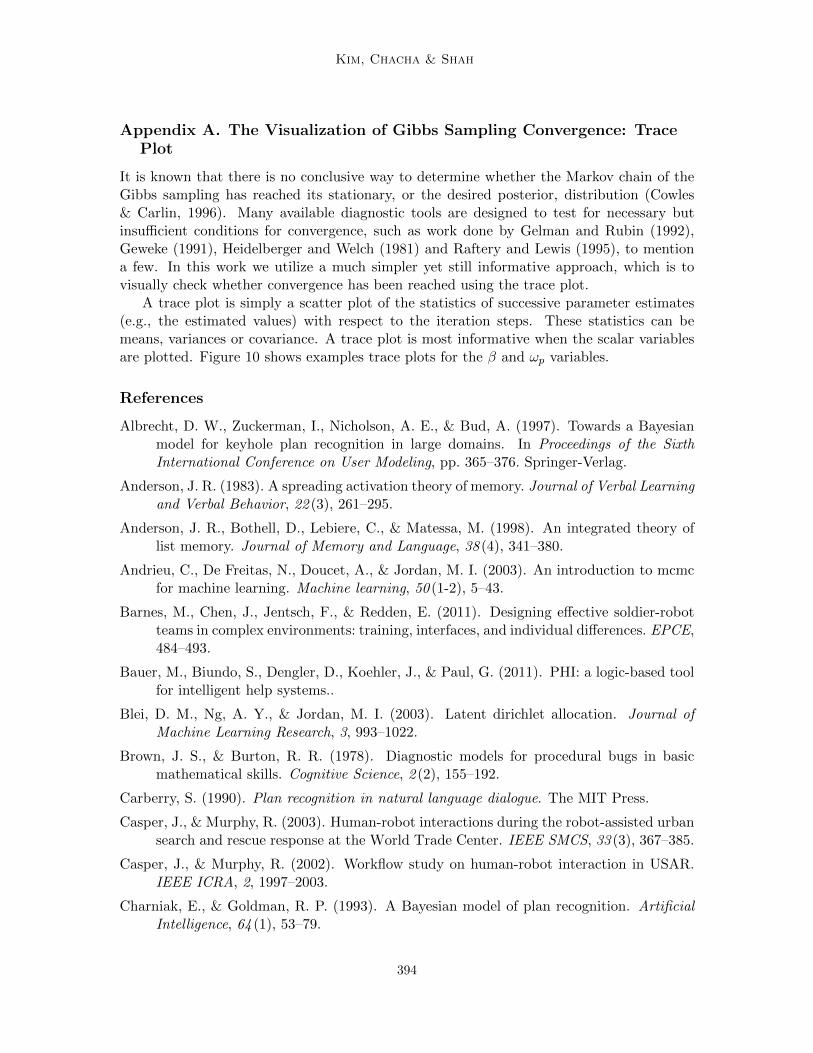
Kim, Chacha & Shah
Appendix A. The Visualization of Gibbs Sampling Convergence: TracePlot
It is known that there is no conclusive way to determine whether the Markov chain of theGibbs sampling has reached its stationary, or the desired posterior, distribution (Cowles& Carlin, 1996). Many available diagnostic tools are designed to test for necessary butinsufficient conditions for convergence, such as work done by Gelman and Rubin (1992),Geweke (1991), Heidelberger and Welch (1981) and Raftery and Lewis (1995), to mentiona few. In this work we utilize a much simpler yet still informative approach, which is tovisually check whether convergence has been reached using the trace plot.
A trace plot is simply a scatter plot of the statistics of successive parameter estimates(e.g., the estimated values) with respect to the iteration steps. These statistics can bemeans, variances or covariance. A trace plot is most informative when the scalar variablesare plotted. Figure 10 shows examples trace plots for the β and ωp variables.
References
Albrecht, D. W., Zuckerman, I., Nicholson, A. E., & Bud, A. (1997). Towards a Bayesianmodel for keyhole plan recognition in large domains. In Proceedings of the SixthInternational Conference on User Modeling, pp. 365–376. Springer-Verlag.
Anderson, J. R. (1983). A spreading activation theory of memory. Journal of Verbal Learningand Verbal Behavior, 22 (3), 261–295.
Anderson, J. R., Bothell, D., Lebiere, C., & Matessa, M. (1998). An integrated theory oflist memory. Journal of Memory and Language, 38 (4), 341–380.
Andrieu, C., De Freitas, N., Doucet, A., & Jordan, M. I. (2003). An introduction to mcmcfor machine learning. Machine learning, 50 (1-2), 5–43.
Barnes, M., Chen, J., Jentsch, F., & Redden, E. (2011). Designing effective soldier-robotteams in complex environments: training, interfaces, and individual differences. EPCE,484–493.
Bauer, M., Biundo, S., Dengler, D., Koehler, J., & Paul, G. (2011). PHI: a logic-based toolfor intelligent help systems..
Blei, D. M., Ng, A. Y., & Jordan, M. I. (2003). Latent dirichlet allocation. Journal ofMachine Learning Research, 3, 993–1022.
Brown, J. S., & Burton, R. R. (1978). Diagnostic models for procedural bugs in basicmathematical skills. Cognitive Science, 2 (2), 155–192.
Carberry, S. (1990). Plan recognition in natural language dialogue. The MIT Press.
Casper, J., & Murphy, R. (2003). Human-robot interactions during the robot-assisted urbansearch and rescue response at the World Trade Center. IEEE SMCS, 33 (3), 367–385.
Casper, J., & Murphy, R. (2002). Workflow study on human-robot interaction in USAR.IEEE ICRA, 2, 1997–2003.
Charniak, E., & Goldman, R. P. (1993). A Bayesian model of plan recognition. ArtificialIntelligence, 64 (1), 53–79.
394
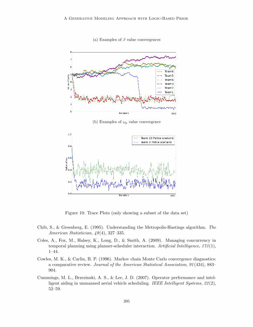
A Generative Modeling Approach with Logic-Based Prior
(a) Examples of β value convergences
(b) Examples of ωp value convergence
Figure 10: Trace Plots (only showing a subset of the data set)
Chib, S., & Greenberg, E. (1995). Understanding the Metropolis-Hastings algorithm. TheAmerican Statistician, 49 (4), 327–335.
Coles, A., Fox, M., Halsey, K., Long, D., & Smith, A. (2009). Managing concurrency intemporal planning using planner-scheduler interaction. Artificial Intelligence, 173 (1),1–44.
Cowles, M. K., & Carlin, B. P. (1996). Markov chain Monte Carlo convergence diagnostics:a comparative review. Journal of the American Statistical Association, 91 (434), 883–904.
Cummings, M. L., Brzezinski, A. S., & Lee, J. D. (2007). Operator performance and intel-ligent aiding in unmanned aerial vehicle scheduling. IEEE Intelligent Systems, 22 (2),52–59.
395

Kim, Chacha & Shah
Di Ciaccio, R., Pullen, J., & Breimyer, P. (2011). Enabling distributed command andcontrol with standards-based geospatial collaboration. IEEE International Conferenceon HST.
FEMA (2014). Federal emergency management agency.. [Online; accessed 3-December-2014].
Fikes, R. E., & Nilsson, N. J. (1972). Strips: A new approach to the application of theoremproving to problem solving. Artificial intelligence, 2 (3), 189–208.
Gal, Y., Reddy, S., Shieber, S. M., Rubin, A., & Grosz, B. J. (2012). Plan recognition inexploratory domains. Artificial Intelligence, 176 (1), 2270–2290.
Geib, C. W., & Goldman, R. P. (2009). A probabilistic plan recognition algorithm basedon plan tree grammars. Artificial Intelligence, 173 (11), 1101–1132.
Geib, C. W., Maraist, J., & Goldman, R. P. (2008). A new probabilistic plan recognitionalgorithm based on string rewriting.. In ICAPS, pp. 91–98.
Gelman, A., & Rubin, D. B. (1992). Inference from iterative simulation using multiplesequences. Statistical Science, 457–472.
Getoor, L., & Mihalkova, L. (2011). Learning statistical models from relational data. In-ternational Conference on Management of Data, 1195–1198.
Geweke, J. (1989). Bayesian inference in econometric models using Monte Carlo integration.Econometrica: Journal of the Econometric Society, 1317–1339.
Geweke, J. (1991). Evaluating the accuracy of sampling-based approaches to the calculationof posterior moments. Federal Reserve Bank of Minneapolis, Research Department.
Goodrich, M. A., Morse, B. S., Engh, C., Cooper, J. L., & Adams, J. A. (2009). Towardsusing UAVs in wilderness search and rescue: Lessons from field trials. InteractionStudies, Special Issue on Robots in the Wild: Exploring Human-Robot Interaction inNaturalistic Environments, 10 (3), 453–478.
Grosz, B. J., & Sidner, C. L. (1990). Plans for discourse. In Cohen, P. R., Morgan,J., & Pollack, M. E. (Eds.), Intentions in Communication, pp. 417–444. MIT Press,Cambridge, MA.
Hastings, W. K. (1970). Monte Carlo sampling methods using Markov chains and theirapplications. Biometrika, 57 (1), 97–109.
Heidelberger, P., & Welch, P. D. (1981). A spectral method for confidence interval generationand run length control in simulations. Communications of the ACM, 24 (4), 233–245.
Holovaty, A., & Kaplan-Moss, J. (2009). The definitive guide to Django: Web developmentdone right. Apress.
Horvitz, E., Breese, J., Heckerman, D., Hovel, D., & Rommelse, K. (1998). The Lumiereproject: Bayesian user modeling for inferring the goals and needs of software users.Proceedings of the Fourteenth Conference on Uncertainty in Artificial Intelligence,256–265.
Howey, R., Long, D., & Fox, M. (2004). Val: Automatic plan validation, continuous effectsand mixed initiative planning using PDDL. IEEE ICTAI, 294–301.
396
A Generative Modeling Approach with Logic-Based Prior
Jones, H., Rock, S., Burns, D., & Morris, S. (2002). Autonomous robots in SWAT applica-tions: Research, design, and operations challenges. AUVSI.
Jurafsky, D., & Martin, J. H. (2000). Speech and Language Processing: An Introduction toNatural Language Processing, Computational Linguistics, and Speech Recognition (1stedition). Prentice Hall PTR, Upper Saddle River, NJ, USA.
Kautz, H. A., Pelavin, R. N., Tenenberg, J. D., & Kaufmann, M. (1991). A formal theoryof plan recognition and its implementation. Reasoning about Plans, 69–125.
Kautz, H. A. (1987). A formal theory of plan recognition. Ph.D. thesis, Bell Laboratories.
Kim, B., Chacha, C. M., & Shah, J. (2013). Inferring robot task plans from human teammeetings: A generative modeling approach with logic-based prior. AAAI.
Kim, J., & Shah, J. A. (2014). Automatic prediction of consistency among team mem-bers’ understanding of group decisions in meetings. In Systems, Man and Cybernetics(SMC), 2014 IEEE International Conference on, pp. 3702–3708. IEEE.
Koomen, P., Punyakanok, V., Roth, D., & Yih, W. (2005). Generalized inference withmultiple semantic role labeling systems. CoNLL, 181–184.
Kruijff, G., Janıcek, M., & Lison, P. (2010). Continual processing of situated dialogue inhuman-robot collaborative activities. In IEEE Ro-Man.
Larochelle, B., Kruijff, G., Smets, N., Mioch, T., & Groenewegen, P. (2011). Establishinghuman situation awareness using a multi-modal operator control unit in an urbansearch & rescue human-robot team. IEEE Ro-Man, 229–234.
Lochbaum, K. E. (1998). A collaborative planning model of intentional structure. Compu-tational Linguistics, 24 (4), 525–572.
Mayfield, J. (1992). Controlling inference in plan recognition. User Modeling and User-Adapted Interaction, 2 (1-2), 55–82.
McDermott, D., Ghallab, M., Howe, A., Knoblock, C., Ram, A., Veloso, M., Weld, D., &Wilkins, D. (1998). PDDL-the planning domain definition language..
Metropolis, N., Rosenbluth, A. W., Rosenbluth, M. N., Teller, A. H., & Teller, E. (1953).Equation of state calculations by fast computing machines. The Journal of ChemicalPhysics, 21, 1087.
Micire, M. (2002). Analysis of robotic platforms used at the World Trade Center disaster.Ph.D. thesis, MS thesis, Department Computer Science Engineering, Univ. SouthFlorida.
Murphy, R. (2004). Human-robot interaction in rescue robotics. IEEE SMCS, 34 (2), 138–153.
Neal, R. M. (2003). Slice sampling. Annals of Statistics, 705–741.
Nguyen, T. A., Kambhampati, S., & Do, M. (2013). Synthesizing robust plans under incom-plete domain models. Advances in Neural Information Processing Systems, 2472–2480.
Palmer, M., Gildea, D., & Xue, N. (2010). Semantic role labeling. Synthesis Lectures onHuman Language Technologies, 3 (1), 1–103.
397
Kim, Chacha & Shah
Pednault, E. P. D. (1987). Formulating Multi-Agent Dynamic-World Problems in the Clas-sical Planning Framework. In Reasoning About Actions and Plans: Proceedings of the1986 Workshop. Morgan Kaufmann Publishers.
Poon, H., & Domingos, P. (2006). Sound and efficient inference with probabilistic anddeterministic dependencies. AAAI, 21 (1), 458.
Poon, H., & Domingos, P. (2009). Unsupervised semantic parsing. EMNLP.
Pradhan, S., Ward, W., Hacioglu, K., Martin, J., & Jurafsky, D. (2004). Shallow semanticparsing using support vector machines. NAACL-HLT, 233.
Pynadath, D. V., & Wellman, M. P. (2000). Probabilistic state-dependent grammars forplan recognition. Proceedings of the Sixteenth conference on Uncertainty in ArtificialIntelligence, 507–514.
Raedt, L. (2008). Probabilistic logic learning. Logical and Relational Learning, 223–288.
Raftery, A. E., & Lewis, S. M. (1995). The number of iterations, convergence diagnosticsand generic metropolis algorithms. In Practical Markov Chain Monte Carlo, 115–130.
Ramırez, M., & Geffner, H. (2009). Plan recognition as planning. Proceedings of the 21stinternational joint conference on Artificial Intelligence, 1778–1783.
Richardson, M., & Domingos, P. (2006). Markov logic networks. Machine learning, 62 (1),107–136.
Ryall, K., Marks, J., & Shieber, S. (1997). An interactive constraint-based system fordrawing graphs. Proceedings of the 10th Annual ACM Symposium on User InterfaceSoftware and Technology, 97–104.
Sadilek, A., & Kautz, H. A. (2010). Recognizing multi-agent activities from GPS data.AAAI.
Singla, P., & Domingos, P. (2007). Markov logic in infinite domains. UAI, 368–375.
Tellex, S., Kollar, T., Dickerson, S., Walter, M., Banerjee, A., Teller, S., & Roy, N. (2011).Understanding natural language commands for robotic navigation and mobile manip-ulation. AAAI.
Weida, R., & Litman, D. (1992). Terminological Reasoning with Constraint Networks andan Application to Plan Recognition.
Whitehill, J. (2013). Understanding ACT-R - an outsider’s perspective. CoRR, 1306.0125.
Zhuo, H. H., Yang, Q., & Kambhampati, S. (2012). Action-model based multi-agent planrecognition. Advances in Neural Information Processing Systems 25, 377–385.
398