INVESTIGATION

Inferring Admixture Histories of Human PopulationsUsing Linkage Disequilibrium

Po-Ru Loh,*,1 Mark Lipson,*,1 Nick Patterson,† Priya Moorjani,†,‡ Joseph K. Pickrell,‡

David Reich,†,‡,2 and Bonnie Berger*,†,2

*Department of Mathematics and Computer Science and Artificial Intelligence Laboratory, Massachusetts Institute of Technology,Cambridge, Massachusetts 02139, †Broad Institute, Cambridge, Massachusetts 02142, and ‡Department of Genetics,

Harvard Medical School, Boston, Massachusetts 02115

ABSTRACT Long-range migrations and the resulting admixtures between populations have been important forces shaping humangenetic diversity. Most existing methods for detecting and reconstructing historical admixture events are based on allele frequencydivergences or patterns of ancestry segments in chromosomes of admixed individuals. An emerging new approach harnesses theexponential decay of admixture-induced linkage disequilibrium (LD) as a function of genetic distance. Here, we comprehensivelydevelop LD-based inference into a versatile tool for investigating admixture. We present a new weighted LD statistic that can be usedto infer mixture proportions as well as dates with fewer constraints on reference populations than previous methods. We define an LD-based three-population test for admixture and identify scenarios in which it can detect admixture events that previous formal testscannot. We further show that we can uncover phylogenetic relationships among populations by comparing weighted LD curvesobtained using a suite of references. Finally, we describe several improvements to the computation and fitting of weighted LD curvesthat greatly increase the robustness and speed of the calculations. We implement all of these advances in a software package, ALDER,which we validate in simulations and apply to test for admixture among all populations from the Human Genome Diversity Project(HGDP), highlighting insights into the admixture history of Central African Pygmies, Sardinians, and Japanese.

ADMIXTURE between previously diverged populationshas been a common feature throughout the evolution

of modern humans and has left significant genetic traces incontemporary populations (Li et al. 2008; Wall et al. 2009;Reich et al. 2009; Green et al. 2010; Gravel et al. 2011;Pugach et al. 2011; Patterson et al. 2012). Resulting patternsof variation can provide information about migrations, de-mographic histories, and natural selection and can also bea valuable tool for association mapping of disease genes inadmixed populations (Patterson et al. 2004).

Recently, a variety of methods have been developed toharness large-scale genotype data to infer admixture events

in the history of sampled populations, as well as to estimatea range of gene flow parameters, including ages, propor-tions, and sources. Some of the most popular approaches,such as STRUCTURE (Pritchard et al. 2000) and principalcomponent analysis (PCA) (Patterson et al. 2006), use clus-tering algorithms to identify admixed populations as inter-mediates in relation to surrogate ancestral populations. Ina somewhat similar vein, local ancestry inference methods(Tang et al. 2006; Sankararaman et al. 2008; Price et al.2009; Lawson et al. 2012) analyze chromosomes of admixedindividuals with the goal of recovering continuous blocksinherited directly from each ancestral population. Becauserecombination breaks down ancestry tracts through succes-sive generations, the time of admixture can be inferred fromthe tract length distribution (Pool and Nielsen 2009; Pugachet al. 2011; Gravel 2012), with the caveat that accurate localancestry inference becomes difficult when tracts are short orthe reference populations used are highly diverged from thetrue mixing populations.

A third class of methods makes use of allele frequencydifferentiation among populations to deduce the presence

Copyright © 2013 by the Genetics Society of Americadoi: 10.1534/genetics.112.147330Manuscript received October 31, 2012; accepted for publication January 25, 2013Available freely online through the author-supported open access option.Supporting information is available online at http://www.genetics.org/lookup/suppl/doi:10.1534/genetics.112.147330/-/DC1.1These authors contributed equally to this work.2Corresponding authors: Department of Genetics, Harvard Medical School, 77 Ave.Louis Pasteur, New Research Bldg., 260I, Boston, MA 02115. E-mail: reich@genetics.med.harvard.edu; and Department of Mathematics, 2-373, Massachusetts Institute ofTechnology, 77 Massachusetts Ave., Cambridge, MA 02139. E-mail: bab@mit.edu

Genetics, Vol. 193, 1233–1254 April 2013 1233

of admixture and estimate parameters, either with likelihood-based models (Chikhi et al. 2001; Wang 2003; Sousa et al.2009; Wall et al. 2009; Laval et al. 2010; Gravel et al. 2011)or with phylogenetic trees built by taking moments of thesite-frequency spectrum over large sets of SNPs (Reich et al.2009; Green et al. 2010; Patterson et al. 2012; Pickrell andPritchard 2012; Lipson et al. 2012). For example, f-statistic-based three- and four-population tests for admixture (Reichet al. 2009; Green et al. 2010; Patterson et al. 2012) arehighly sensitive in the proper parameter regimes and whenthe set of sampled populations sufficiently represents the phy-logeny. One disadvantage of drift-based statistics, however, isthat because the rate of genetic drift depends on populationsize, these methods do not allow for inference of the time thathas elapsed since admixture events.

Finally, Moorjani et al. (2011) recently proposed a fourthapproach, using associations between pairs of loci to makeinference about admixture, which we further develop in thisarticle. In general, linkage disequilibrium (LD) in a populationcan be generated by selection, genetic drift, or populationstructure, and it is eroded by recombination. Within a homo-geneous population, steady-state neutral LD is maintained bythe balance of drift and recombination, typically becomingnegligible in humans at distances of more than a few hundredkilobases (Reich et al. 2001; International HapMap Consor-tium 2007). Even if a population is currently well mixed,however, it can retain longer-range admixture LD (ALD) fromadmixture events in its history involving previously separatedpopulations. ALD is caused by associations between nearbyloci co-inherited on an intact chromosomal block from one ofthe ancestral mixing populations (Chakraborty and Weiss1988). Recombination breaks down these associations, leav-ing a signature of the time elapsed since admixture that canbe probed by aggregating pairwise LD measurements throughan appropriate weighting scheme; the resulting weighted LDcurve (as a function of genetic distance) exhibits an exponen-tial decay with rate constant giving the age of admixture(Moorjani et al. 2011; Patterson et al. 2012). This approachto admixture dating is similar in spirit to strategies based onlocal ancestry, but LD statistics have the advantage of a simplemathematical form that facilitates error analysis.

In this article, we comprehensively develop LD-basedadmixture inference, extending the methodology to severalnovel applications that constitute a versatile set of tools forinvestigating admixture. We first propose a cleaner func-tional form of the underlying weighted LD statistic andprovide a precise mathematical development of its proper-ties. As an immediate result of this theory, we observe thatour new weighted LD statistic can be used to infer mixtureproportions as well as dates, extending the results of Pickrellet al. (2012). Moreover, such inference can still be per-formed (albeit with reduced power) when data are availablefrom only the admixed population and one surrogate ancestralpopulation, whereas all previous techniques require at leasttwo such reference populations. As a second application, wepresent an LD-based three-population test for admixture

with sensitivity complementary to the three-populationf-statistic test (Reich et al. 2009; Patterson et al. 2012) andcharacterize the scenarios in which each is advantageous.We further show that phylogenetic relationships betweentrue mixing populations and present-day references can beinferred by comparing weighted LD curves using weightsderived from a suite of reference populations. Finally, wedescribe several improvements to the computation and fit-ting of weighted LD curves: we show how to detect con-founding LD from sources other than admixture, improvingthe robustness of our methods in the presence of sucheffects, and we present a novel fast Fourier transform-based algorithm for weighted LD computation that reducestypical run times from hours to seconds. We implement allof these advances in a software package, ALDER (Admix-ture-induced Linkage Disequilibrium for EvolutionaryRelationships).

We demonstrate the performance of ALDER by using it totest for admixture among all HGDP populations (Li et al.2008) and compare its results to those of the three-populationtest, highlighting the sensitivity trade-offs of each approach.We further illustrate our methodology with case studies ofCentral African Pygmies, Sardinians, and Japanese, reveal-ing new details that add to our understanding of admixtureevents in the history of each population.

Methods

Properties of weighted admixture LD

In this section we introduce a weighted LD statistic that usesthe decay of LD to detect signals of admixture given SNPdata from an admixed population and reference popula-tions. This statistic is similar to, but has an importantdifference from, the weighted LD statistic used in ROLLOFF(Moorjani et al. 2011; Patterson et al. 2012). The formula-tion of our statistic is particularly important in allowing us touse the amplitude (i.e., y-intercept) of the weighted LDcurve to make inferences about history. We begin by deriv-ing quantitative mathematical properties of this statistic thatcan be used to infer admixture parameters.

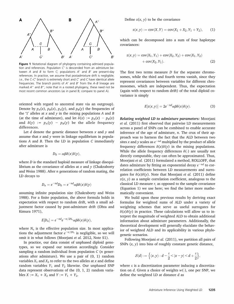
Basic model and notation: We will primarily considera point-admixture model in which a population C9 descendsfrom a mixture of populations A and B to form C, n gener-ations ago, in proportions a + b = 1, followed by randommating (Figure 1). As we discuss later, we can assume forour purposes that the genetic drift between C and C9 isnegligible, and hence we will simply refer to the descendantpopulation as C as well; we will state whether we mean thepopulation immediately after admixture vs. n generationslater when there is any risk of ambiguity. We are interestedin the properties of the LD in population C induced by ad-mixture. Consider two biallelic, neutrally evolving SNPs xand y, and for each SNP call one allele ‘0’ and the other ‘1’(this assignment is arbitrary; ‘0’ and ‘1’ do not need to be

1234 P.-R. Loh et al.

oriented with regard to ancestral state via an outgroup).Denote by pA(x), pB(x), pA(y), and pB(y) the frequencies ofthe ‘1’ alleles at x and y in the mixing populations A and B(at the time of admixture), and let d(x) := pA(x) 2 pB(x)and d(y) := pA(y) 2 pB(y) be the allele frequencydifferences.

Let d denote the genetic distance between x and y andassume that x and y were in linkage equilibrium in popula-tions A and B. Then the LD in population C immediatelyafter admixture is

D0 ¼ abdðxÞdðyÞ;

where D is the standard haploid measure of linkage disequi-librium as the covariance of alleles at x and y (Chakrabortyand Weiss 1988). After n generations of random mating, theLD decays to

Dn ¼ e2ndD0 ¼ e2ndabdðxÞdðyÞ

assuming infinite population size (Chakraborty and Weiss1988). For a finite population, the above formula holds inexpectation with respect to random drift, with a small ad-justment factor caused by post-admixture drift (Ohta andKimura 1971),

E½Dn� ¼ e2nde2n=2NeabdðxÞdðyÞ;

where Ne is the effective population size. In most applica-tions the adjustment factor e2n=2Ne is negligible, so we willomit it in what follows (Moorjani et al. 2012, Note S1).

In practice, our data consist of unphased diploid geno-types, so we expand our notation accordingly. Considersampling a random individual from population C (n gener-ations after admixture). We use a pair of {0, 1} randomvariables X1 and X2 to refer to the two alleles at x and definerandom variables Y1 and Y2 likewise. Our unphased SNPdata represent observations of the {0, 1, 2} random varia-bles X := X1 + X2 and Y := Y1 + Y2.

Define z(x, y) to be the covariance

zðx; yÞ :¼ covðX; YÞ ¼ covðX1 þ X2; Y1 þ Y2Þ; (1)

which can be decomposed into a sum of four haplotypecovariances:

zðx; yÞ ¼ covðX1; Y1Þ þ covðX2; Y2Þ þ covðX1; Y2Þþ covðX2; Y1Þ: (2)

The first two terms measure D for the separate chromo-somes, while the third and fourth terms vanish, since theyrepresent covariances between variables for different chro-mosomes, which are independent. Thus, the expectation(again with respect to random drift) of the total diploid co-variance is simply

E½zðx; yÞ� ¼ 2e2ndabdðxÞdðyÞ: (3)

Relating weighted LD to admixture parameters: Moorjaniet al. (2011) first observed that pairwise LD measurementsacross a panel of SNPs can be combined to enable accurateinference of the age of admixture, n. The crux of their ap-proach was to harness the fact that the ALD between twosites x and y scales as e2nd multiplied by the product of allelefrequency differences d(x)d(y) in the mixing populations.While the allele frequency differences d(�) are usually notdirectly computable, they can often be approximated. Thus,Moorjani et al. (2011) formulated a method, ROLLOFF, thatdates admixture by fitting an exponential decay e2nd to cor-relation coefficients between LD measurements and surro-gates for d(x)d(y). Note that Moorjani et al. (2011) definez(x, y) as a sample correlation coefficient, analogous to theclassical LD measure r, as opposed to the sample covariance(Equation 1) we use here; we find the latter more mathe-matically convenient.

We build upon these previous results by deriving exactformulas for weighted sums of ALD under a variety ofweighting schemes that serve as useful surrogates ford(x)d(y) in practice. These calculations will allow us to in-terpret the magnitude of weighted ALD to obtain additionalinformation about admixture parameters. Additionally, thetheoretical development will generally elucidate the behav-ior of weighted ALD and its applicability in various phylo-genetic scenarios.

Following Moorjani et al. (2011), we partition all pairs ofSNPs (x, y) into bins of roughly constant genetic distance,

SðdÞ :¼nðx; yÞ : d2 e

2, jx2 yj, dþ e

2

o;

where e is a discretization parameter inducing a discretiza-tion on d. Given a choice of weights w(�), one per SNP, wedefine the weighted LD at distance d as

Figure 1 Notational diagram of phylogeny containing admixed popula-tion and references. Population C9 is descended from an admixture be-tween A and B to form C; populations A9 and B9 are present-dayreferences. In practice, we assume that postadmixture drift is negligible;i.e., the C–C9 branch is extremely short and C9 and C have identical allelefrequencies. The branch points of A9 and B9 from the A–B lineage aremarked A$ and B$; note that in a rooted phylogeny, these need not bemost recent common ancestors (as in panel B; compare to panel A).

Admixture Inference Using Weighted LD 1235

aðdÞ :¼P

SðdÞzðx; yÞwðxÞwð yÞ

jSðdÞj :

Assume first that our weights are the true allele fre-quency differences in the mixing populations, i.e., w(x) =d(x) for all x. Applying Equation 3,

E½aðdÞ� ¼ E

"PSðdÞzðx; yÞdðxÞdðyÞjSðdÞj

#

¼P

SðdÞ2abE

hdðxÞ2 dðyÞ2

ie2nd

jSðdÞj¼ 2abF2ðA;BÞ2e2nd;

(4)

where F2(A, B) is the expected squared allele frequencydifference for a randomly drifting neutral allele, as definedin Reich et al. (2009) and Patterson et al. (2012). Thus, a(d)has the form of an exponential decay as a function of d, withtime constant n giving the date of admixture.

In practice, we must compute an empirical estimator ofa(d) from a finite number of sampled genotypes. Say wehave a set of m diploid admixed samples from populationC indexed by i = 1, . . ., m, and denote their genotypes atsites x and y by xi, yi 2 {0, 1, 2}. Also assume we have somefinite number of reference individuals from A and B withempirical mean allele frequencies pAð�Þ and pBð�Þ. Then ourestimator is

aðdÞ :¼P

SðdÞbcovðX; YÞð pAðxÞ2 pBðxÞÞð pAð yÞ2 pBð yÞÞ

jSðdÞj ;

(5)

where

bcovðX; YÞ ¼ 1m2 1

Xmi¼1

�xi 2 �x

��yi 2 �y

�

is the usual unbiased sample covariance, so the expectationover the choice of samples satisfies E½aðdÞ� ¼ aðdÞ (assumingno background LD, so the ALD in population C is indepen-dent of the drift processes producing the weights).

The weighted sumP

SðdÞzðx; yÞwðxÞwðyÞ is a naturalquantity to use for detecting ALD decay and is common toour weighted LD statistic aðdÞ and previous formulations ofROLLOFF. Indeed, for SNP pairs (x, y) at a fixed distance d,we can think of Equation 3 as providing a simple linear re-gression model between LD measurements z(x, y) and allelefrequency divergence products d(x)d(y). In practice, the lin-ear relation is made noisy by random sampling, as notedabove, but the regression coefficient 2abe2nd can be inferredby combining measurements from many SNP pairs (x, y). Infact, the weighted sum

PSðdÞzðx; yÞdðxÞdðyÞ in the numera-

tor of Equation 5 is precisely the numerator of the least-squares estimator of the regression coefficient, which is the

formulation of ROLLOFF given in Moorjani et al. (2012, NoteS1). Note that measurements of z(x, y) cannot be combineddirectly without a weighting scheme, as the sign of the LD canbe either positive or negative; additionally, the weights tendto preserve signal from ALD while depleting contributionsfrom other forms of LD.

Up to scaling, our ALDER formulation is roughly equiv-alent to the regression coefficient formulation of ROLLOFF(Moorjani et al. 2012, Note S1). In contrast, the originalROLLOFF statistic (Patterson et al. 2012) computed a corre-lation coefficient between z(x, y) and w(x)w(y) over S(d).However, the normalization term

ffiffiffiffiffiffiffiffiffiffiffiffiffiffiffiffiffiffiffiffiffiPSðdÞzðx; yÞ

2q

in the denom-

inator of the correlation coefficient can exhibit an unwantedd-dependence that biases the inferred admixture date if theadmixed population has undergone a strong bottleneck(Moorjani et al. 2012, Note S1) or in the case of recentadmixture and large sample sizes. Beyond correcting thedate bias, the aðdÞ curve that ALDER computes has the ad-vantage of a simple form for its amplitude in terms of mean-ingful quantities, providing us additional leverage on admixtureparameters. Additionally, we will show that aðdÞ can becomputed efficiently via a new fast Fourier transform-based algorithm.

Using weights derived from diverged reference popula-tions: In the above development, we set the weights w(x) toequal the allele frequency differences d(x) between the truemixing populations A and B. In practice, in the absence ofDNA samples from past populations, it is impossible to mea-sure historical allele frequencies from the time of mixture, soinstead, we substitute reference populations A9 and B9 thatare accessible, setting wðxÞ ¼ d9ðxÞ :¼ pA9ðxÞ2 pB9ðxÞ. Ina given data set, the closest surrogates A9 and B9 may besomewhat diverged from A and B, so it is important to un-derstand the consequences for the weighted LD a(d).

We show in Appendix A that with reference populationsA9 and B9 in place of A and B, Equation 4 for the expectedweighted LD curve changes only slightly, becoming

E½aðdÞ� ¼ 2abF2�A$;B$

�2e2nd; (6)

where A$ and B$ are the branch points of A9 and B9 on theA–B lineage (Figure 1). Notably, the curve still has the formof an exponential decay with time constant n (the age ofadmixture), albeit with its amplitude (and therefore signal-to-noise ratio) attenuated according to how far A$ and B$are from the true ancestral mixing populations. Drift alongthe A9 2 A$ and B9 2 B$ branches likewise decreases signal-to-noise but in the reverse manner: higher drift on thesebranches makes the weighted LD curve noisier but doesnot change its expected amplitude (Supporting Information,Figure S1; see Appendix C for additional discussion). Asabove, given a real data set containing finite samples, wecompute an estimator aðdÞ analogous to Equation 5 that hasthe same expectation (over sampling and drift) as the ex-pectation of a(d) with respect to drift (Equation 6).

1236 P.-R. Loh et al.

Using the admixed population as one reference: WeightedLD can also be computed with only a single referencepopulation by using the admixed population as the otherreference (Pickrell et al. 2012, Supplement Sect. 4). Assum-ing first that we know the allele frequencies of the ancestralmixing population A and the admixed population C, theformula for the expected curve becomes

E½aðdÞ� ¼ 2ab3F2ðA;BÞ2e2nd: (7)

Using C itself as one reference population and R9 as theother reference (which could branch anywhere between Aand B), the formula for the amplitude is slightly more com-plicated, but the curve retains the e2nd decay (Figure S2):

E½aðdÞ� ¼ 2ab�aF2

�A;R$

�2bF2

�B;R$

��2e2nd: (8)

Derivations of these formulas are given in Appendix A.A subtle but important technical issue arises when com-

puting weighted LD with a single reference. In this case, thetrue weighted LD statistic is

aðdÞ ¼ covðX; YÞðmx 2 pðxÞÞðmy 2 pðyÞÞ;

where

mx ¼ apAðxÞ þ bpBðxÞ and my ¼ apAð yÞ þ bpBð yÞ

are the mean allele frequencies of the admixed population(ignoring drift) and p(�) denotes allele frequencies of thereference population. Here a(d) cannot be estimated accu-rately by the naïve formula

bcovðX; YÞðmx 2 pðxÞÞðmy 2 pð yÞÞ;

which is the natural analog of (5). The difficulty is that thecovariance term and the weights both involve the allelefrequencies mx and my; thus, while the standard estimatorsfor each term are individually unbiased, their product is a bi-ased estimate of the weighted LD.

Pickrell et al. (2012) circumvents this problem by parti-tioning the admixed samples into two groups, designatingone group for use as admixed representatives and the otheras a reference population; this method eliminates bias butreduces statistical power. We instead compute a polyachestatistic (File S1) that provides an unbiased estimator aðdÞof the weighted LD with maximal power.

Affine term in weighted LD curve from population sub-structure: Weighted LD curves computed on real popula-tions often exhibit a nonzero horizontal asymptote contraryto the exact exponential decay formulas we have derivedabove. Such behavior can be caused by assortative matingresulting in subpopulations structured by ancestry percent-age in violation of our model. We show in Appendix A that ifwe instead model the admixed population as consisting ofrandomly mating subpopulations with heterogeneous amounts

a—now a random variable—of mixed ancestry, our equationsfor the curves take the form

E½aðdÞ� ¼ Me2nd þ K; (9)

where M is a coefficient representing the contribution ofadmixture LD and K is an additional constant produced bysubstructure. Conveniently, however, the sum M + K/2 sat-isfies the same equations that the coefficient of the exponen-tial does in the homogeneous case: adjusting Equation 6 forpopulation substructure gives

M þ K=2 ¼ 2abF2�A$;B$

�2(10)

for two-reference weighted LD, and in the one-referencecase, modifying Equation 8 gives

M þ K=2 ¼ 2ab�aF2

�A;R$

�2bF2

�B;R$

��2: (11)

For brevity, from here on we will take the amplitude of anexponential-plus-affine curve to mean M + K/2.

Admixture inference using weighted LD

We now describe how the theory we have developed can beused to investigate admixture. We detail novel techniquesthat use weighted LD to infer admixture parameters, test foradmixture, and learn about phylogeny.

Inferring admixture dates and fractions using one or tworeference populations: As noted above, our ALDER formu-lation of weighted LD hones the original two-referenceadmixture dating technique of ROLLOFF (Moorjani et al.2011), correcting a possible bias (Moorjani et al. 2012, NoteS1), and the one-reference technique (Pickrell et al. 2012),improving statistical power. Pickrell et al. (2012) also ob-served that weighted LD can be used to estimate ancestralmixing fractions. We further develop this application now.

The main idea is to treat our expressions for theamplitude of the weighted LD curve as equations that canbe solved for the ancestry fractions a and b = 1 2 a. Firstconsider two-reference weighted LD. Given samples from anadmixed population C and reference populations A9 and B9,we compute the curve aðdÞ and fit it as an exponential decayplus affine term: aðdÞ � Me2nd þ K. Let a0 :¼ M þ K=2 de-note the amplitude of the curve. Then Equation 10 gives usa quadratic equation that we can solve to obtain an estimatea of the mixture fraction a,

2að12 aÞF2�A$;B$

�2 ¼ a0;

assuming we can estimate F2(A$, B$)2. Typically the branch-point populations A$ and B$ are unavailable, but their F2distance can be computed by means of an admixture tree(Lipson et al. 2012; Patterson et al. 2012; Pickrell andPritchard 2012). A caveat of this approach is that a and1 2 a produce the same amplitude and cannot be distin-guished by this method alone; additionally, the inversion

Admixture Inference Using Weighted LD 1237

problem is ill-conditioned near a = 0.5, where the deriva-tive of the quadratic vanishes.

The situation is more complicated when using theadmixed population as one reference. First, the amplituderelation from Equation 11 gives a quartic equation in a:

2að12 aÞ�aF2�A;R$�2ð12aÞF2�B;R$

��2 ¼ a0:

Second, the F2 distances involved are in general not possibleto calculate by solving allele frequency moment equations(Lipson et al. 2012; Patterson et al. 2012). In the special casethat one of the true mixing populations is available as a ref-erence, however—i.e., R9 = A—Pickrell et al. (2012) dem-onstrated that mixture fractions can be estimated muchmore easily. From Equation 7, the expected amplitude ofthe curve is 2ab3F2(A, B)2. On the other hand, assumingno drift in C since the admixture, allele frequencies in Care given by weighted averages of allele frequencies in Aand B with weights a and b; thus, the squared allele fre-quency differences from A to B and C satisfy

F2ðA;CÞ ¼ b2F2ðA;BÞ;

and F2(A, C) is estimable directly from the sample data.Combining these relations, we can obtain our estimate a

by solving the equation

2a=ð12 aÞ ¼ a0=F2ðA;CÞ2: (12)

In practice, the true mixing population A is not available forsampling, but a closely related population A9 may be. In thiscase, the value of a given by Equation 12 with A9 in place ofA is a lower bound on the true mixture fraction a (seeAppendix A for theoretical development and Results for sim-ulations exploring the tightness of the bound). This bound-ing technique is the most compelling of the above mixturefraction inference approaches, as prior methods cannot per-form such inference with only one reference population. Incontrast, when more references are available, moment-based admixture tree-fitting methods, for example, readilyestimate mixture fractions (Lipson et al. 2012; Pattersonet al. 2012; Pickrell and Pritchard 2012). In such cases webelieve that existing methods are more robust than LD-basedinference, which suffers from the degeneracy of solutionsnoted above; however, the weighted LD approach can provideconfirmation based on a different genetic mechanism.

Testing for admixture: Thus far, we have taken it as giventhat the population C of interest is admixed and developedmethods for inferring admixture parameters by fittingweighted LD curves. Now we consider the question ofwhether weighted LD can be used to determine whetheradmixture occurred in the first place. We develop aweighted LD-based formal test for admixture that is broadlyanalogous to the drift-based three-population test (Reichet al. 2009; Patterson et al. 2012) but sensitive in differentscenarios.

A complication of interpreting weighted LD is that certaindemographic events other than admixture can also producepositive weighted LD that decays with genetic distance,particularly in the one-reference case. Specifically, if pop-ulation C has experienced a recent bottleneck or anextended period of low population size, it may containlong-range LD. Furthermore, this LD typically has some cor-relation with allele frequencies in C; consequently, usingC as one reference in the weighting scheme produces a spu-rious weighted LD signal.

In the two-reference case, LD from reduced populationsize in C is generally washed out by the weighting schemeassuming the reference populations A9 and B9 are not toogenetically similar to C. The reason is that the weightsdð�Þ ¼ pA9 ð�Þ2 pB9 ð�Þ arise from drift between A9 and B9 thatis independent of demographic events producing LD in C(beyond genetic distances that are so short that the popula-tions share haplotypes descended without recombinationfrom their common ancestral haplotype). Thus, observinga two-reference weighted LD decay curve is generally goodevidence that population C is admixed. There is still a caveat,however. If C and one of the references, say A9, share a recentpopulation bottleneck, then the bottleneck-induced LD in Ccan be correlated to the allele frequencies of A9, resultingonce again in spurious weighted LD. In fact, the one-refer-ence example mentioned above is the limiting case A9 = C ofthis situation.

With these considerations in mind, we propose an LD-based three-population test for admixture that includesa series of pre-tests safeguarding against the pathologicaldemographies that can produce a non-admixture weightedLD signal. We outline the test now; details are in Appendix B.Given a population C to test for admixture and references A9and B9, the main test is whether the observed weightedLD aðdÞ using A9 2 B9 weights is positive and well-fit byan exponential decay curve. We estimate a jackknife-basedp-value by leaving out each chromosome in turn and refit-ting the weighted LD as an exponential decay; the jackknifethen gives us a standard error on the fitting parameters—namely, the amplitude and the decay constant—that we useto measure the significance of the observed curve.

The above procedure allows us to determine whetherthere is sufficient signal in the weighted LD curve to rejectthe null hypothesis (under which aðdÞ is random “colored”noise in the sense that it contains autocorrelation). How-ever, in order to conclude that the curve is the result ofadmixture, we must rule out the possibility that it is beingproduced by demography unrelated to admixture. We there-fore apply the following pre-test procedure. First, we deter-mine the distance to which LD in C is significantly correlatedwith LD in either A9 or B9; to minimize signal from shareddemography, we subsequently ignore data from SNP pairs atdistances smaller than this correlation threshold. Then, wecompute one-reference weighted LD curves for population Cwith A9–C and B9–C weights and check that the curves arewell-fit as exponential decays. In the case that C is actually

1238 P.-R. Loh et al.

admixed between populations related to A9 and B9, the one-reference A9–C and B9–C curves pick up the same e2nd admix-ture LD decay signal. If C is not admixed but has experienceda shared bottleneck with A9 (producing false-positive admix-ture signals from the A9 – B9 and B9–C curves), however, theA9–C weighting scheme is unlikely to produce a weighted LDcurve, especially when fitting beyond the LD correlationthreshold.

This test procedure is intended to be conservative, so thata population C identified as admixed can strongly be as-sumed to be so, whereas if C is not identified as admixed,we are less confident in claiming that C has experienced noadmixture whatsoever. In situations where distinguishingadmixture from other demography is particularly difficult,the test will err on the side of caution; for example, even if Cis admixed, the test may fail to identify C as admixed if it hasalso experienced a bottleneck. Also, if a reference A9 sharessome of the same admixture history as C or is simply veryclosely related to C, the pre-test will typically identify long-range correlated LD and deem A9 an unsuitable reference touse for testing admixture. The behavior of the test and pre-test criteria are explored in detail with coalescent simula-tions in Appendix C.

Learning about phylogeny: Given a triple of populations (C;A9, B9), our test can identify admixture in the test populationC, but what does this imply about the relationship of popula-tions A9 and B9 to C? As with the drift-based three-populationtest, test results must be interpreted carefully: even if C isadmixed, this does not necessarily mean that the referencepopulations A9 and B9 are closely related to the true mixingpopulations. However, computing weighted LD curves witha suite of different references can elucidate the phylogeny ofthe populations involved, since our amplitude Equations 10and 11 provide information about the locations on the phy-logeny at which the references diverge from the true mixingpopulations.

More precisely, in the notation of Figure 1, the amplitudeof the two-reference weighted LD curve is 2abF2(A$, B$)2,which is maximized when A$ = A and B$ = B andis minimized when A$ = B$. So, for example, we can fixA9 and compute curves for a variety of references B9; thelarger the resulting amplitude, the closer the branch pointB$ is to B. In the one-reference case, as the reference R9 isvaried, the amplitude 2ab(aF2(A, R$)2 bF2(B, R$))2 tracesout a parabola that starts at 2ab3F2(A, B)2 when R$ = A,decreases to a minimum value of 0, and increases again to2a3bF2(A, B)2 when R$ = B (Figure S2). Here, the proce-dure is more qualitative because the branches F2(A, R$) andF2(B, R$) are less directly useful and the mixture propor-tions a and b may not be known.

Implementation of ALDER

We now describe some more technical details of the ALDERsoftware package in which we have implemented our weightedLD methods.

Fast Fourier transform algorithm for computing weightedLD: We developed a novel algorithm that algebraicallymanipulates the weighted LD statistic into a form that canbe computed using a fast Fourier transform (FFT), dramat-ically speeding up the computation (File S2). The algebraictransformation is made possible by the simple form (Equa-tion 5) of our weighted LD statistic along with a geneticdistance discretization procedure that is similar spirit toROLLOFF (Moorjani et al. 2011) but subtly different: in-stead of binning the contributions of SNP pairs (x, y) bydiscretizing the genetic distance |x 2 y| = d, we discretizethe genetic map positions x and y themselves (using a defaultresolution of 0.05 cM) (Figure S3). For two-referenceweighted LD, the resulting FFT-based algorithm that weimplemented in ALDER has computational cost that is ap-proximately linear in the data size; in practice, it ran threeorders of magnitude faster than ROLLOFF on typical datasets we analyzed.

Curve fitting: We fit discretized weighted LD curves aðdÞ asMe2nd þ K from Equation 9, using least-squares to find best-fit parameters. This procedure is similar to ROLLOFF, butALDER makes two important technical advances that signif-icantly improve the robustness of the fitting. First, ALDERdirectly estimates the affine term K that arises from thepresence of subpopulations with differing ancestry percen-tages by using interchromosome SNP pairs that are effectivelyat infinite genetic distance (Appendix A). The algorithmicadvances we implement in ALDER enable efficient computa-tion of the average weighted LD over all pairs of SNPs ondifferent chromosomes, giving K and, importantly, eliminat-ing one parameter from the exponential fitting. In practice,we have observed that ROLLOFF fits are sometimes sensitiveto the maximum inter-SNP distance d to which the weightedLD curve is computed and fit; ALDER eliminates thissensitivity.

Second, because background LD is present in realpopulations at short genetic distances and confounds theALD signal (interfering with parameter estimates or pro-ducing spurious signal entirely), it is important to fitweighted LD curves starting only at a distance beyondwhich background LD is negligible. ROLLOFF used a fixedthreshold of d . 0.5 cM, but some populations have longer-range background LD (e.g., from bottlenecks), and more-over, if a reference population is closely related to the testpopulation, it can produce a spurious weighted LD signaldue to recent shared demography. ALDER therefore esti-mates the extent to which the test population shares corre-lated LD with the reference(s) and fits only the weighted LDcurve beyond this minimum distance as in our test for ad-mixture (Appendix B).

We estimate standard errors on parameter estimates byperforming a jackknife over the autosomes used in theanalysis, leaving out each in turn. Note that the weighted LDmeasurements from individual pairs of SNPs that go into thecomputed curve aðdÞ are not independent of each other;

Admixture Inference Using Weighted LD 1239

however, the contributions of different chromosomes canreasonably be assumed to be independent.

Data sets

We primarily applied our weighted LD techniques to a dataset of 940 individuals in 53 populations from the CEPH–Hu-man Genome Diversity Cell Line Panel (HGDP) (Rosenberget al. 2002) genotyped on an Illumina 650K SNP array (Liet al. 2008). To study the effect of SNP ascertainment, we alsoanalyzed the same HGDP populations genotyped on the Affy-metrix Human Origins Array (Patterson et al. 2012). For someanalyses we also included HapMap Phase 3 data (Interna-tional HapMap Consortium 2010) merged either with theIllumina HGDP data set, leaving �600,000 SNPs, or withthe Indian data set of Reich et al. (2009) including 16 Anda-man Islanders (9 Onge and 7 Great Andamanese), leaving�500,000 SNPs.

We also constructed simulated admixed chromosomesfrom 112 CEU and 113 YRI phased HapMap individualsusing the following procedure, described in Moorjani et al.(2011). Given desired ancestry proportions a and b, the agen of the point admixture, and the number m of admixedindividuals to simulate, we built each admixed chromosomeas a composite of chromosomal segments from the sourcepopulations, choosing breakpoints via a Poisson process withrate constant n, and sampling blocks at random according tothe specified mixture fractions. We stipulated that no indi-vidual haplotype could be reused at a given locus among them simulated individuals, preventing unnaturally long iden-tical-by-descent segments but effectively eliminating postad-mixture genetic drift. For the short time scales we study(admixture occurring 200 or fewer generations ago), thisapproximation has little impact. We used this method tomaintain some of the complications inherent in real data.

Results

Simulations

First, we demonstrate the accuracy of several forms ofinference from ALDER on simulated data. We generatedsimulated genomes for mixture fractions of 75% YRI/25%CEU and 90% YRI/10% CEU and admixture dates of 10, 20,50, 100, and 200 generations ago. For each mixture scenariowe simulated 40 admixed individuals according to theprocedure above.

We first investigated the admixture dates estimated byALDER using a variety of reference populations drawn fromthe HGDP with varying levels of divergence from the truemixing populations. On the African side, we used HGDPYoruba (21 samples; essentially the same population asHapMap YRI) and San (5 samples); on the European side,we used French (28 samples; very close to CEU), Han (34samples), and Papuan (17 samples). We computed two-reference weighted LD curves using pairs of references, onefrom each group, as well as one-reference curves using the

simulated population as one reference and each of the aboveHGDP populations as the other.

For the 75% YRI mixture, estimated dates are nearly allaccurate to within 10% (Table S1). The noise levels of thefitted dates (estimated by ALDER using the jackknife) arethe lowest for the Yoruba–French curve, as expected, fol-lowed by the one-reference curve with French, consistentwith the admixed population being mostly Yoruba. The sit-uation is similar but noisier for the 90% YRI mixture (TableS2); in this case, the one-reference signal is quite weak withYoruba and undetectable with San as the reference, due tothe scaling of the amplitude (Equation 11) with the cube ofthe CEU mixture fraction.

We also compared fitted amplitudes of the weighted LDcurves for the same scenarios to those predicted byEquations 10 and 11; the accuracy trends are similar (TableS3 and Table S4). Finally, we tested Equation 12 for bound-ing mixture proportions using one-reference weighted LDamplitudes. We computed lower bounds on the Europeanancestry fraction using French, Russian, Sardinian, andKalash as successively more diverged references. Asexpected, the bounds are tight for the French referenceand grow successively weaker (Table S5 and Table S6).We also tried lower-bounding the African ancestry usingone-reference curves with an African reference. In general,we expect lower bounds computed for the major ancestryproportion to be much weaker (Appendix A), and indeed wefind this to be the case, with the only slightly diverged Man-denka population producing extremely weak bounds. Anadded complication is that the Mandenka are an admixedpopulation with a small amount of West Eurasian ancestry(Price et al. 2009), which is not accounted for in the ampli-tude formulas we use here.

Another notable feature of ALDER is that, to a muchgreater extent than f-statistic methods, its inference qualityimproves with more samples from the admixed test popula-tion. As a demonstration of this, we simulated a larger set of100 admixed individuals as above, for both 75% YRI/25%CEU and 90% YRI/10% CEU scenarios, and compared thedate estimates obtained on subsets of 5–100 of these indi-viduals with two different reference pairs (Table S7 andTable S8). With larger sample sizes, the estimates becomealmost uniformly more accurate, with smaller standarderrors. By contrast, we observed that while using a verysmall sample size (say 5) for the reference populations doescreate noticeable noise, using 20 samples already gives al-lele frequency estimates accurate enough that adding morereference samples has only minimal effects on the perfor-mance of ALDER. This is similar to the phenomenon that theprecision of f-statistics does not improve appreciably withmore than a moderate number of samples and is due tothe inherent variability in genetic drift among different loci.

Robustness

A challenge of weighted LD analysis is that owing to variouskinds of model violation, the parameters of the exponential

1240 P.-R. Loh et al.

fit of an observed curve aðdÞ may depend on the startingdistance d0 from which the curve is fit. We therefore ex-plored the robustness of the fitting parameters to the choiceof d0 in a few scenarios (Figure 2). First, in a simulated75%/25% YRI–CEU admixture 50 generations ago, we findthat the decay constant and amplitude are both highly ro-bust to varying d0 from 0.5 to 2.0 cM (Figure 2, top). Thisresult is not surprising because our simulated example rep-resents a true point admixture with minimal background LDin the admixed population.

In practice, we expect some dependence on d0 due tobackground LD or longer-term admixture (either continu-ously over a stretch of time or in multiple waves). Both ofthese tend to increase the weighted LD for smaller values ofd relative to an exact exponential curve, so that estimates ofthe decay constant and amplitude decrease as we increasethe fitting start point d0; the extent to which this effectoccurs depends on the extent of the model violation. Westudied the d0 dependence for two example admixed pop-ulations, HGDP Uygur and HapMap Maasai (MKK). For

Uygur, the estimated decay constants and amplitudes arefairly robust to the start point of the fitting, varying roughlyby 610% (Figure 2, middle). In contrast, the estimates forMaasai vary dramatically, decreasing by a factor of .2 as d0is increased from 0.5 to 2.0 cM (Figure 2, bottom). Thisbehavior is likely due to multiple-wave admixture in thegenetic history of the Maasai; indeed, it is visually evidentthat the weighted LD curve for Maasai deviates from anexponential fit (Figure 2) and is in fact better fit as a sumof exponentials. (See Figure S4 and Appendix C for furthersimulations exploring continuous admixture.)

It is also important to consider the possibility of SNPascertainment bias, as in any study based on allele frequen-cies. We believe that for weighted LD, ascertainment biascould have modest effects on the amplitude, which dependson F2 distances (Lipson et al. 2012; Patterson et al. 2012),but does not affect the estimated date. Running ALDER ona suite of admixed populations in the HGDP under a varietyof ascertainment schemes suggests that admixture date esti-mates are indeed quite stable to ascertainment (Table S9).

Figure 2 Dependence of dateestimates and weighted LDamplitudes on fitting start point.Rows correspond to three testscenarios: simulated 75% YRI/25% CEU mixture 50 genera-tions ago with Yoruba–Frenchweights (A–C); Uygur with Han–French weights (D–F); HapMapMaasai with Yoruba–Frenchweights (G–I). (A, D, and G) Theweighted LD curve aðdÞ (blue)with best-fit exponential decaycurve (red), fit starting fromd0 = 0.5 cM. The middle andright columns show the date es-timate (B, E, H) and amplitude(C, F, I) as a function of d0. (Wenote that our date estimates forUygur are somewhat more re-cent than those in Pattersonet al. 2012, most likely becauseof our direct estimate of theaffine term in the weighted LDcurve.)

Admixture Inference Using Weighted LD 1241

Meanwhile, the amplitudes of the LD curves can scale sub-stantially when computed under different SNP ascertain-ments, but their relative values are different only forextreme cases of African vs. non-African test populationsunder African vs. non-African ascertainment (Table S10; cf.Patterson et al. 2012, Table 2).

Admixture test results for HGDP populations

To compare the sensitivity of our LD-based test for admix-ture to the f-statistic-based three-population test, we ranboth ALDER and the three-population test on all triples ofpopulations in the HGDP. Interestingly, while the tests con-cur on the majority of the populations they identify asadmixed, each also identifies several populations asadmixed that the other does not (Table 1), showing thatthe tests have differing sensitivity to different admixturescenarios.

Admixture identified only by ALDER: The three-populationtest loses sensitivity primarily as a result of drift subsequentto splitting from the references’ lineages. More precisely,using the notation of Figure 1, the three-population teststatistic f3(C; A9, B9) estimates the sum of two directly com-peting terms: 2abF2(A$, B$), the negative quantity arisingfrom admixture that we wish to detect, and a2F2(A$, A) +b2F2(B$, B) + F2(C, C$), a positive quantity from the “off-tree” drift branches. If the latter term dominates, the three-population test will fail to detect admixture regardless of thestatistical power available. For example, Melanesians areonly found to be admixed according to the ALDER test;

the inability of the three-population test to identify themas admixed is likely due to long off-tree drift from the Pap-uan branch prior to admixture. The situation is similar forthe Pygmies, for whom we do not have two close referencesavailable.

Small mixture fractions also diminish the size of theadmixture term 2abF2(A, B) relative to the off-tree drift,and we believe this effect along with postadmixture driftmay be the reason Sardinians are detected as admixed onlyby ALDER. In the case of the San, who have a small amountof Bantu admixture (Pickrell et al. 2012), the small mixturefraction may again play a role, along with the lack of a ref-erence population closely related to the preadmixture San,meaning that using existing populations incurs long off-treedrift.

Admixture identified only by the three-population test:There are also multiple reasons why the three-populationtest can identify admixture when ALDER does not. For theHGDP European populations in this category (Table 1), thethree-population test is picking up a signal of admixtureidentified by Patterson et al. (2012) and interpreted asa large-scale admixture event in Europe involving Neolithicfarmers closely related to present-day Sardinians and anancient northern Eurasian population. This mixture likelybegan quite anciently (e.g., 7000–9000 years ago when ag-riculture arrived in Europe; Bramanti et al. 2009; Soareset al. 2010; Pinhasi et al. 2012), and because admixtureLD breaks down as e2nd, where n is the age of admixture,there is nearly no LD left for ALDER to harness beyond the

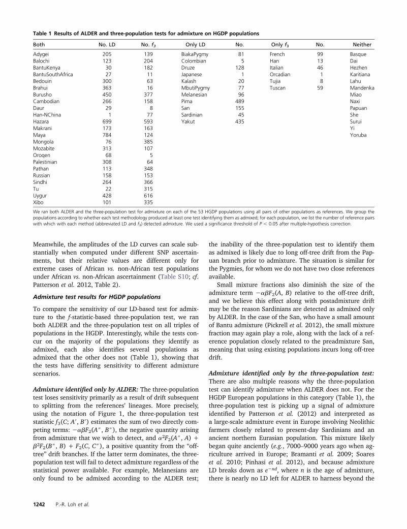
Table 1 Results of ALDER and three-population tests for admixture on HGDP populations

Both No. LD No. f3 Only LD No. Only f3 No. Neither

Adygei 205 139 BiakaPygmy 81 French 99 BasqueBalochi 123 204 Colombian 5 Han 13 DaiBantuKenya 30 182 Druze 128 Italian 46 HezhenBantuSouthAfrica 27 11 Japanese 1 Orcadian 1 KaritianaBedouin 300 63 Kalash 20 Tujia 8 LahuBrahui 363 16 MbutiPygmy 77 Tuscan 59 MandenkaBurusho 450 377 Melanesian 96 MiaoCambodian 266 158 Pima 489 NaxiDaur 29 8 San 155 PapuanHan-NChina 1 77 Sardinian 45 SheHazara 699 593 Yakut 435 SuruiMakrani 173 163 YiMaya 784 124 YorubaMongola 76 385Mozabite 313 107Oroqen 68 5Palestinian 308 64Pathan 113 348Russian 158 153Sindhi 264 366Tu 22 315Uygur 428 616Xibo 101 335

We ran both ALDER and the three-population test for admixture on each of the 53 HGDP populations using all pairs of other populations as references. We group thepopulations according to whether each test methodology produced at least one test identifying them as admixed; for each population, we list the number of reference pairswith which with each method (abbreviated LD and f3) detected admixture. We used a significance threshold of P , 0.05 after multiple-hypothesis correction.

1242 P.-R. Loh et al.

correlation threshold d0. An additional factor that may in-hibit LD-based testing is that to prevent false-positive iden-tifications of admixture, ALDER typically eliminates referencepopulations that share LD (and in particular, admixture his-tory) with the test population, whereas the three-populationtest can use such references.

To summarize, the ALDER and three-population testsboth analyze a test population for admixture using tworeferences, but they detect signal based on different “geneticclocks.” The three-population test uses signal from geneticdrift, which can detect quite old admixture but must over-come a counteracting contribution from postadmixture andoff-tree drift. The LD-based test uses recombination, whichis relatively unaffected by small population size-inducedlong drift and has no directly competing effect, but has lim-ited power to detect chronologically old admixtures becauseof the rapid decay of the LD curve. Additionally, as discussedabove in the context of simulation results, the LD-based testmay be better suited for large data sets, since its power isenhanced more by the availability of many samples. Thetests are thus complementary and both valuable. (See FigureS5 and Appendix C for further exploration.)

Case studies

We now present detailed results for several human pop-ulations, all of which ALDER identifies as admixed but arenot found by the three-population test (Table 1). We inferdates of admixture and in some cases gain additional histor-ical insights.

Pygmies: Both Central African Pygmy populations in theHGDP, the Mbuti and Biaka, show evidence of admixture(Table 1), about 28 6 4 generations (800 years) ago forMbuti and 38 6 4 generations (1100 years) ago for Biaka,estimated using San and Yoruba as reference populations(Figure 3, A and C). The intrapopulation heterogeneity islow, as demonstrated by the negligible affine terms. In eachcase, we also generated weighted LD curves with the Pygmypopulation itself as one reference and a variety of secondreferences. We found that using French, Han, or Yoruba asthe second reference gave very similar amplitudes, but theamplitude was significantly smaller with the other Pygmypopulation or San as the second reference (Figure 3, Band D). Using the amplitudes with Yoruba, we estimatedmixture fractions of at least 15.9 6 0.9% and 28.8 61.4% Yoruba-related ancestry (lower bounds) for Mbutiand Biaka, respectively.

The phylogenetic interpretation of the relative ampli-tudes is complicated by the fact that the Pygmy populations,used as references, are themselves admixed, but a plausiblecoherent explanation is as follows (see Figure 3E). We sur-mise that a proportion b (bounds given above) of Bantu-related gene flow reached the native Pygmy populationson the order of 1000 years ago. The common ancestors ofYoruba or non-Africans with the Bantu population are genet-ically not very different from Bantu, due to high historical

population sizes (branching at positions X1 and X2 in Figure3E). Thus, the weighted LD amplitudes using Yoruba or non-Africans as second references are nearly 2a3bF2(A, B)2,where B denotes the admixing Bantu population. Meanwhile,San and Western (resp. Eastern) Pygmies split from theBantu–Mbuti (resp. Biaka) branch toward the middle orthe opposite side from Bantu (X3 and X4), giving a smalleramplitude (Figure S2).

Our results are in agreement with previous studies thathave found evidence of gene flow from agriculturalists toPygmies (Quintana-Murci et al. 2008; Verdu et al. 2009;Patin et al. 2009; Jarvis et al. 2012). Quintana-Murci et al.(2008) suggested based on mtDNA evidence in Mbuti thatgene flow ceased several thousand years ago, but more re-cently, Jarvis et al. (2012) found evidence of admixture inWestern Pygmies, with a local-ancestry-inferred block-length distribution of 3.1 6 4.6 Mb (mean and standarddeviation), consistent with our estimated dates.

Sardinians: We detect a very small proportion of sub-Saharan African ancestry in Sardinians, which our ALDERtests identified as admixed (Table 1 and Figure 4A). To in-vestigate further, we computed weighted LD curves withSardinian as the test population and all pairs of the HapMapCEU, YRI, and CHB populations as references (Table 2). Weobserved an abnormally large amount of shared long-rangeLD in chromosome 8, likely because of an extended inver-sion segregating in Europeans (Price et al. 2008), so weomitted it from these analyses. The CEU–YRI curve has thelargest amplitude, suggesting both that the LD present isdue to admixture and that the small non-European ancestrycomponent, for which we estimated a lower bound of 0.6 60.2%, is from Africa. (For this computation we used single-reference weighted LD with YRI as the reference, fitting thecurve after 1.2 cM to reduce confounding effects from cor-related LD that ALDER detected between Sardinian andCEU. Changing the starting point of the fit does not quali-tatively affect the results.) The existence of a weighted LDdecay curve with CHB and YRI as references provides fur-ther evidence that the LD is not simply due to a populationbottleneck or other nonadmixture sources, as does the factthat our estimated dates from all three reference pairs areroughly consistent at about 40 generations (1200 years)ago. Our findings thus confirm the signal of African ancestryin Sardinians reported in Moorjani et al. (2011). The date,small mixture proportion, and geography are consistent witha small influx of migrants from North Africa, who them-selves traced only a fraction of their ancestry ultimately tosub-Saharan Africa, consistent with the findings of Dupanloupet al. (2004).

Japanese: Genetic studies have suggested that present-dayJapanese are descended from admixture between two wavesof settlers, responsible for the Jomon and Yayoi cultures(Hammer and Horai 1995; Hammer et al. 2006; Rasteiroand Chikhi 2009). We also observed evidence of admixture

Admixture Inference Using Weighted LD 1243

in Japanese, and while our ability to learn about the historywas limited by the absence of a close surrogate for the orig-inal Paleolithic mixing population, we were able to takeadvantage of the one-reference inference capabilities ofALDER. More precisely, among our tests using all pairs ofHGDP populations as references (Table 1), one referencepair, Basque and Yakut, produced a passing test for Japa-nese. However, as we have noted, the reference populationsneed not be closely related to the true mixing populations,and we believe that in this case this seemingly odd referencepair arises as the only passing test because the data set lacksa close surrogate for Jomon.

In the absence of a reference on the Jomon side, wecomputed single-reference weighted LD using HapMap JPTas the test population and JPT–CHB weights, which conferthe advantage of larger sample sizes (Figure 4B). Theweighted LD curve displays a clear decay, yielding an esti-mate of 45 6 6 generations, or about 1300 years, as the ageof admixture. To our knowledge, this is the first time ge-nome-wide data have been used to date admixture in Japa-nese. As with previous estimates based on coalescence ofY-chromosome haplotypes (Hammer et al. 2006), our dateis consistent with the archeologically attested arrival ofthe Yayoi in Japan �2300 years ago (we suspect that our

Figure 3 Weighted LD curves forMbuti using San and Yoruba asreference populations (A) and us-ing Mbuti itself as one referenceand several different secondreferences (B), and analogouscurves for Biaka (C and D). Ge-netic distances are discretized in-to bins at 0.05 cM resolution.Data for each curve are plottedand fit starting from the corre-sponding ALDER-computed LDcorrelation thresholds. Differentamplitudes of one-referencecurves (B and D) imply differentphylogenetic positions of thereferences relative to the truemixing populations (i.e., differentsplit points X$i ), suggestinga sketch of a putative admixturegraph (E). Relative branch lengthsare qualitative, and the true rootis not necessarily as depicted.

1244 P.-R. Loh et al.

estimate is from later than the initial arrival because admix-ture may not have happened immediately or may have takenplace over an extended period of time). Based on the am-plitude of the curve, we also obtain a (likely very conserva-tive) genome-wide lower bound of 41 6 3% “Yayoi”ancestry using Equation 12 (under the reasonable assump-tion that Han Chinese are fairly similar to the Yayoi popu-lation). It is important to note that the observation ofa single-reference weighted LD curve is not sufficient evi-dence to prove that a population is admixed, but the exis-tence of a pair of references with which the ALDER testidentified Japanese as admixed, combined with previouswork and the lack of any signal of reduced population size,makes us confident that our inferences are based on truehistorical admixture.

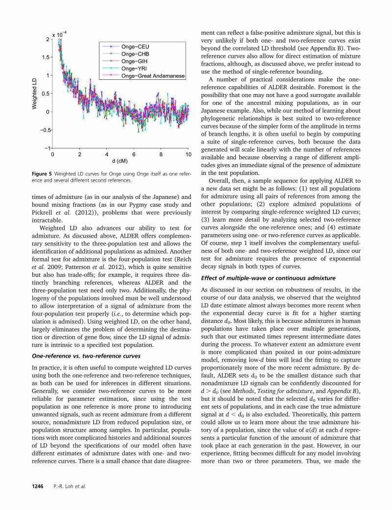
Onge: Finally, we provide a cautionary example of weightedLD decay curves arising from demography and not admixture.

We observed distinct weighted LD curves when analyzing theOnge, an indigenous population of the Andaman Islands.However, this curve is present only when using Ongethemselves as one reference; moreover, the amplitude isindependent of whether CEU, CHB, YRI, GIH (HapMapGujarati), or Great Andamanese is used as the secondreference (Figure 5), as expected if the weighted LD is dueto correlation between LD and allele frequencies in the testpopulation alone (and independent of the reference allelefrequencies). Correspondingly, ALDER’s LD-based test doesnot identify Onge as admixed using any pair of these refer-ences. Thus, while we cannot definitively rule out admix-ture, the evidence points toward internal demography (lowpopulation size) as the cause of the elevated LD, consistentwith the current census of ,100 Onge individuals.

Discussion

Strengths of weighted LD for admixture inference

The statistics underlying weighted LD are quite simple,making the formula for the expectation of aðdÞ, as well asthe noise and other errors from our inference procedure,relatively easy to understand. By contrast, local ancestry-based admixture dating methods (e.g., Pool and Nielsen(2009) and Gravel (2012)) are sensitive to imperfect ances-try inference, and it is difficult to trace the error propagationto understand the ultimate effect on inferred admixtureparameters. Similarly, the wavelet method of Pugach et al.(2011) uses reference populations to perform (fuzzy) ances-try assignment in windows, for which error analysis ischallenging.

Another strength of our weighted LD methodology is thatit has relatively low requirements on the quality andquantity of reference populations. Our theory tells us exactlyhow the statistic behaves for any reference populations, nomatter how diverged they are from the true ancestral mixingpopulations. In contrast, the accuracy of results fromclustering and local ancestry methods is dependent on thequality of the reference populations used in ways that aredifficult to characterize. On the quantity side, previousapproaches to admixture inference require a surrogate foreach ancestral population, whereas as long as one isconfident that the signal is truly from admixture, weightedLD can be used with only one available reference to infer

Figure 4 Weighted LD curves for HGDP Sardinian using Italian–Yorubaweights (A) and HapMap Japanese (JPT) using JPT itself as one referenceand HapMap Han Chinese in Beijing (CHB) as the second reference (B).The exponential fits are performed starting at 1 cM and 1.2 cM, respec-tively, as selected by ALDER based on detected correlated LD.

Table 2 Amplitudes and dates from weighted LD curves forSardinian using various reference pairs

Ref 1 Ref 2 Weighted LD amplitude Date estimate

CEU YRI 0.00003192 6 0.00000903 48 6 10CHB YRI 0.00001738 6 0.00000679 34 6 8CEU CHB 0.00000873 6 0.00000454 52 6 21

Data are shown from ALDER fits to weighted LD curves computed using Sardinianas the test population and pairs of HapMap CEU, YRI, and CHB as the references.Date estimates are in generations. We omitted chromosome 8 from the analysisbecause of anomalous long-range LD. Curves aðdÞ were fit for d . 1.2 cM, theextent of LD correlation between Sardinian and CEU computed by ALDER.

Admixture Inference Using Weighted LD 1245

times of admixture (as in our analysis of the Japanese) andbound mixing fractions (as in our Pygmy case study andPickrell et al. (2012)), problems that were previouslyintractable.

Weighted LD also advances our ability to test foradmixture. As discussed above, ALDER offers complemen-tary sensitivity to the three-population test and allows theidentification of additional populations as admixed. Anotherformal test for admixture is the four-population test (Reichet al. 2009; Patterson et al. 2012), which is quite sensitivebut also has trade-offs; for example, it requires three dis-tinctly branching references, whereas ALDER and thethree-population test need only two. Additionally, the phy-logeny of the populations involved must be well understoodto allow interpretation of a signal of admixture from thefour-population test properly (i.e., to determine which pop-ulation is admixed). Using weighted LD, on the other hand,largely eliminates the problem of determining the destina-tion or direction of gene flow, since the LD signal of admix-ture is intrinsic to a specified test population.

One-reference vs. two-reference curves

In practice, it is often useful to compute weighted LD curvesusing both the one-reference and two-reference techniques,as both can be used for inferences in different situations.Generally, we consider two-reference curves to be morereliable for parameter estimation, since using the testpopulation as one reference is more prone to introducingunwanted signals, such as recent admixture from a differentsource, nonadmixture LD from reduced population size, orpopulation structure among samples. In particular, popula-tions with more complicated histories and additional sourcesof LD beyond the specifications of our model often havedifferent estimates of admixture dates with one- and two-reference curves. There is a small chance that date disagree-

ment can reflect a false-positive admixture signal, but this isvery unlikely if both one- and two-reference curves existbeyond the correlated LD threshold (see Appendix B). Two-reference curves also allow for direct estimation of mixturefractions, although, as discussed above, we prefer instead touse the method of single-reference bounding.

A number of practical considerations make the one-reference capabilities of ALDER desirable. Foremost is thepossibility that one may not have a good surrogate availablefor one of the ancestral mixing populations, as in ourJapanese example. Also, while our method of learning aboutphylogenetic relationships is best suited to two-referencecurves because of the simpler form of the amplitude in termsof branch lengths, it is often useful to begin by computinga suite of single-reference curves, both because the datagenerated will scale linearly with the number of referencesavailable and because observing a range of different ampli-tudes gives an immediate signal of the presence of admixturein the test population.

Overall, then, a sample sequence for applying ALDER toa new data set might be as follows: (1) test all populationsfor admixture using all pairs of references from among theother populations; (2) explore admixed populations ofinterest by comparing single-reference weighted LD curves;(3) learn more detail by analyzing selected two-referencecurves alongside the one-reference ones; and (4) estimateparameters using one- or two-reference curves as applicable.Of course, step 1 itself involves the complementary useful-ness of both one- and two-reference weighted LD, since ourtest for admixture requires the presence of exponentialdecay signals in both types of curves.

Effect of multiple-wave or continuous admixture

As discussed in our section on robustness of results, in thecourse of our data analysis, we observed that the weightedLD date estimate almost always becomes more recent whenthe exponential decay curve is fit for a higher startingdistance d0. Most likely, this is because admixtures in humanpopulations have taken place over multiple generations,such that our estimated times represent intermediate datesduring the process. To whatever extent an admixture eventis more complicated than posited in our point-admixturemodel, removing low-d bins will lead the fitting to captureproportionately more of the more recent admixture. By de-fault, ALDER sets d0 to be the smallest distance such thatnonadmixture LD signals can be confidently discounted ford . d0 (see Methods, Testing for admixture, and Appendix B),but it should be noted that the selected d0 varies for differ-ent sets of populations, and in each case the true admixturesignal at d , d0 is also excluded. Theoretically, this patterncould allow us to learn more about the true admixture his-tory of a population, since the value of a(d) at each d repre-sents a particular function of the amount of admixture thattook place at each generation in the past. However, in ourexperience, fitting becomes difficult for any model involvingmore than two or three parameters. Thus, we made the

Figure 5 Weighted LD curves for Onge using Onge itself as one refer-ence and several different second references.

1246 P.-R. Loh et al.

decision to restrict ourselves to assuming a single-point ad-mixture, fit for a principled threshold d . d0, accepting thatthe inferred date n represents some form of average valueover the true history.

Other possible complications

In our derivations, we have assumed implicitly that themixing populations and the reference populations are relatedthrough a simple tree. However, it may be that their history ismore complicated, for example, involving additional admix-tures. In this case, our formulas for the amplitude of the ALDcurve will be inaccurate if, for example, A and A9 have differ-ent admixture histories. However, if our assumptions are vi-olated only by events occurring before the divergencesbetween the mixing populations and the corresponding refer-ences, then the amplitude will be unaffected. Moreover, nomatter what the population history is, as long as A and B arefree of measurable LD (so that our assumption of indepen-dence of alleles conditional on a single ancestry is valid),there will be no effect on the estimated date of admixture.

Conclusions and future directions

In this study, we have shown how LD generated by pop-ulation admixture can be a powerful tool for learning abouthistory, extending previous work that showed how it can beused for estimating dates of mixture (Moorjani et al. 2011;Patterson et al. 2012). We have developed a new suite oftools, implemented in the ALDER software package, thatsubstantially increases the speed of admixture LD analysis,improves the robustness of admixture date inference, andexploits the amplitude of LD as a novel source of informa-tion about history. In particular, (a) we show how admixtureLD can be leveraged into a formal test for mixture that cansometimes find evidence of admixture not detectable byother methods, (b) we show how to estimate mixture pro-portions, and (c) we show that we can even use this infor-mation to infer phylogenetic relationships. A limitation ofALDER at present, however, is that it is designed for a modelof pulse admixture between two ancestral populations. Im-portant directions for future work will be to generalize theseideas to make inferences about the time course of admixturein the case that it took place over a longer period of time(Pool and Nielsen 2009; Gravel 2012) and to study multi-way admixture. In addition, it would be valuable to be ableto use the information from admixture LD to constrain mod-els of history for multiple populations simultaneously, eitherby extending ALDER itself or by using LD-based test resultsin conjunction with methods for fitting phylogenies incorpo-rating admixture (Lipson et al. 2012; Patterson et al. 2012;Pickrell and Pritchard, 2012).

Software

Executable and C++ source files for our ALDER softwarepackage are available online at the Berger and Reich Labwebsites: http://groups.csail.mit.edu/cb/alder/, http://genetics.med.harvard.edu/reich/Reich_Lab/Software.html.

Acknowledgments

We are grateful to the reviewer for many suggestions thatsubstantially increased the quality of this manuscript. M.L.and P.L. acknowledge National Science Foundation (NSF)Graduate Research Fellowship support. P.L. was also par-tially supported by National Institutes of Health (NIH)training grant 5T32HG004947-04 and the Simons Founda-tion. N.P., J.P. and D.R. are grateful for support from NSFHOMINID grant 1032255 and NIH grant GM100233.

Literature Cited

Bramanti, B., M. Thomas, W. Haak, M. Unterlaender, P. Joreset al., 2009 Genetic discontinuity between local hunter–gatherers and Central Europe’s first farmers. Science 326(5949): 137–140.

Chakraborty, R., and K. Weiss, 1988 Admixture as a tool for findinglinked genes and detecting that difference from allelic associ-ation between loci. Proc. Natl. Acad. Sci. USA 85(23): 9119–9123.

Chen, G., P. Marjoram, and J. Wall, 2009 Fast and flexible simu-lation of DNA sequence data. Genome Res. 19(1): 136–142.

Chikhi, L., M. Bruford, and M. Beaumont, 2001 Estimation ofadmixture proportions: a likelihood-based approach using Mar-kov chain Monte Carlo. Genetics 158: 1347–1362.

Davies, R., 1977 Hypothesis testing when a nuisance parame-ter is present only under the alternative. Biometrika 64(2):247–254.

Dupanloup, I., G. Bertorelle, L. Chikhi, andG. Barbujani, 2004 Estimatingthe impact of prehistoric admixture on the genome of Europeans. Mol.Biol. Evol. 21(7): 1361–1372.

Gravel, S., 2012 Population genetics models of local ancestry.Genetics 191: 607–619.

Gravel, S., B. Henn, R. Gutenkunst, A. Indap, G. Marth et al.,2011 Demographic history and rare allele sharing among hu-man populations. Proc. Natl. Acad. Sci. USA 108(29): 11983–11988.

Green, R., J. Krause, A. Briggs, T. Maricic, U. Stenzel et al., 2010 Adraft sequence of the Neandertal genome. Science 328(5979):710–722.

Hammer, M., and S. Horai, 1995 Y chromosomal DNA variationand the peopling of Japan. Am. J. Hum. Genet. 56(4): 951–962.

Hammer, M., T. Karafet, H. Park, K. Omoto, S. Harihara et al.,2006 Dual origins of the Japanese: common ground forhunter–gatherer and farmer Y chromosomes. J. Hum. Genet.51(1): 47–58.

International HapMap Consortium, 2007 A second generation hu-man haplotype map of over 3.1 million SNPs. Nature 449(7164): 851–861.

International HapMap Consortium, 2010 Integrating commonand rare genetic variation in diverse human populations. Nature467(7311): 52–58.

Jarvis, J., L. Scheinfeldt, S. Soi, C. Lambert, L. Omberg et al.,2012 Patterns of ancestry, signatures of natural selection,and genetic association with stature in western African Pygmies.PLoS Genet. 8(4): e1002641.

Laval, G., E. Patin, L. Barreiro, and L. Quintana-Murci,2010 Formulating a historical and demographic model of re-cent human evolution based on resequencing data from non-coding regions. PLoS ONE 5(4): e10284.

Lawson, D., G. Hellenthal, S. Myers, and D. Falush, 2012 Inferenceof population structure using dense haplotype data. PLoS Genet.8(1): e1002453.

Admixture Inference Using Weighted LD 1247

Li, J., D. Absher, H. Tang, A. Southwick, A. Casto et al.,2008 Worldwide human relationships inferred from genome-wide patterns of variation. Science 319(5866): 1100–1104.

Lipson, M., P. Loh, A. Levin, D. Reich, N. Patterson et al.,2012 Efficient moment-based inference of admixture param-eters and sources of gene flow, arXiv arXiv:1212.2555 (inpress).

Moorjani, P., N. Patterson, J. Hirschhorn, A. Keinan, L. Haoet al., 2011 The history of African gene flow into South-ern Europeans, Levantines, and Jews. PLoS Genet. 7(4):e1001373.

Moorjani, P., N. Patterson, P. Loh, M. Lipson, P. Kisfali et al.,2012 Reconstructing Roma history from genome-wide data.,arXiv arXiv:1212.1696 (in press).

Ohta, T., and M. Kimura, 1971 Linkage disequilibrium betweentwo segregating nucleotide sites under the steady flux of muta-tions in a finite population. Genetics 68: 571–580.

Patin, E., G. Laval, L. Barreiro, A. Salas, O. Semino et al.,2009 Inferring the demographic history of African farmersand Pygmy hunter–gatherers using a multilocus resequencingdata set. PLoS Genet. 5(4): e1000448.

Patterson, N., N. Hattangadi, B. Lane, K. Lohmueller, D. Hafleret al., 2004 Methods for high-density admixture mapping ofdisease genes. Am. J. Hum. Genet. 74(5): 979–1000.

Patterson, N., A. Price, and D. Reich, 2006 Population structureand eigenanalysis. PLoS Genet. 2(12): e190.

Patterson, N., P. Moorjani, Y. Luo, S. Mallick, N. Rohland et al.,2012 Ancient admixture in human history. Genetics 192:1065–1093.

Pickrell, J., and J. Pritchard, 2012 Inference of population splitsand mixtures from genome-wide allele frequency data. PLoSGenet. 8(11): e1002967.

Pickrell, J., N. Patterson, C. Barbieri, F. Berthold, L. Gerlach et al.,2012 The genetic prehistory of southern Africa. Nat. Commun.3(1): 1143.

Pinhasi, R., M. Thomas, M. Hofreiter, M. Currat, and J. Burger,2012 The genetic history of Europeans. Trends Genet. 28(10): 496–505.

Pool, J., and R. Nielsen, 2009 Inference of historical changes inmigration rate from the lengths of migrant tracts. Genetics 181:711–719.

Price, A., M. Weale, N. Patterson, S. Myers, A. Need et al.,2008 Long-range LD can confound genome scans in admixedpopulations. Am. J. Hum. Genet. 83(1): 132–135.

Price, A., A. Tandon, N. Patterson, K. Barnes, N. Rafaels et al.,2009 Sensitive detection of chromosomal segments of dis-

tinct ancestry in admixed populations. PLoS Genet. 5(6):e1000519.

Pritchard, J., M. Stephens, and P. Donnelly, 2000 Inference ofpopulation structure using multilocus genotype data. Genetics155: 945–959.

Pugach, I., R. Matveyev, A. Wollstein, M. Kayser, and M. Stoneking,2011 Dating the age of admixture via wavelet transform anal-ysis of genome-wide data. Genome Biol. 12(2): R19.

Quintana-Murci, L., H. Quach, C. Harmant, F. Luca, B. Massonnetet al., 2008 Maternal traces of deep common ancestry andasymmetric gene flow between Pygmy hunter–gatherers andBantu-speaking farmers. Proc. Natl. Acad. Sci. USA 105(5):1596.

Rasteiro, R., and L. Chikhi, 2009 Revisiting the peopling of Japan:an admixture perspective. J. Hum. Genet. 54(6): 349–354.

Reich, D., M. Cargill, S. Bolk, J. Ireland, P. Sabeti et al.,2001 Linkage disequilibrium in the human genome. Nature411(6834): 199–204.

Reich, D., K. Thangaraj, N. Patterson, A. Price, and L. Singh,2009 Reconstructing Indian population history. Nature 461(7263): 489–494.

Rosenberg, N., J. Pritchard, J. Weber, H. Cann, K. Kidd et al.,2002 Genetic structure of human populations. Science 298(5602): 2381–2385.

Sankararaman, S., S. Sridhar, G. Kimmel, and E. Halperin,2008 Estimating local ancestry in admixed populations.Am. J. Hum. Genet. 82(2): 290–303.

Soares, P., A. Achilli, O. Semino, W. Davies, V. Macaulay et al.,2010 The archaeogenetics of Europe. Curr. Biol. 20(4): R174–R183.

Sousa, V., M. Fritz, M. Beaumont, and L. Chikhi, 2009 ApproximateBayesian computation without summary statistics: the case ofadmixture. Genetics 181: 1507–1519.

Tang, H.,M. Coram, P.Wang, X. Zhu, andN. Risch, 2006 Reconstructinggenetic ancestry blocks in admixed individuals. Am. J. Hum. Genet. 79(1): 1–12.

Verdu, P., F. Austerlitz, A. Estoup, R. Vitalis, M. Georges et al.,2009 Origins and genetic diversity of Pygmy hunter–gatherersfrom western Central Africa. Curr. Biol. 19(4): 312–318.

Wall, J., K. Lohmueller, and V. Plagnol, 2009 Detecting an-cient admixture and estimating demographic parameters inmultiple human populations. Mol. Biol. Evol. 26(8): 1823–1827.

Wang, J., 2003 Maximum-likelihood estimation of admixture pro-portions from genetic data. Genetics 164: 747–765.

Communicating editor: J. Wall

Appendix A: Derivations of Weighted LD Formulas

Expected Weighted LD Using Two Diverged Reference Populations

We now derive Equation 6 for the expected weighted LD (with respect to random drift) using references A9 and B9 in placeof A and B, retaining the notation of Figure 1. Let A9 and B9 have allele frequencies pA9ð�Þ and pB9ð�Þ, and letd9ð�Þ :¼ pA9ð�Þ2 pB9ð�Þ denote the allele frequency divergences with which we weight the LD z(x, y), giving the two-sitestatistic

aðdÞ :¼ zðx; yÞd9ðxÞd9ðyÞ:

[For brevity, we drop the binning procedure of averaging over SNP pairs (x, y) at distance |x2 y| � d here.] The value of therandom variable z(x, y) is affected by sampling noise as well as genetic drift between A and B, while the random variablesd9(x) and d9(y) are outcomes of genetic drift between A9 and B9. These random variables are uncorrelated conditional on theallele frequencies of x and y in A$ and B$. We also assume that x and y are distant enough to have negligible background LDand hence the drifts at the two sites are independent. We then have

1248 P.-R. Loh et al.

E½aðdÞ� ¼ Ehzðx; yÞd9ðxÞd9ðyÞ

i¼ E

hE�zðx; yÞd9ðxÞd9ðyÞjpA$ðxÞ; pB$ðxÞ; pA$ðyÞ; pB$ðyÞ

�i¼ E

h2abdðxÞdðyÞd9ðxÞd9ðyÞe2nd

i¼ 2abe2ndF2

�A$;B$

�2;

where in the last step the relation E[d(x)d9(x)] = E[d(y)d9(y)] = F2(A$, B$) follows from the fact that the intersection of thedrift paths d(�) and d9(�) is the branch between A$ and B$ (Reich et al. 2009).

Expected Weighted LD Using One Diverged Reference Population

Using the admixed population C as one reference and a population A9 as the other, we have pC(�) = apA(�) + bpB(�)(assuming negligible postadmixture drift), giving weights

dA9Cð�Þ ¼ pA9ð�Þ2apAð�Þ2bpBð�Þ ¼ adA9Að�Þ þ bdA9B ð�Þ;

where dPQ denotes the allele frequency difference between populations P and Q. Arguing as above, the expected weighted LDis given by

E½aðdÞ� ¼ Eh2abdðxÞdðyÞdA9CðxÞdA9CðyÞe2nd

i:

To complete the calculation, we compute

E½dð�ÞdA9Cð�Þ� ¼ aE½dð�ÞdA9Að�Þ� þ bE½dð�ÞdA9Bð�Þ�:

For the first term, the intersection of the A–B and A9–A drift paths is the A–A$ branch, so E½dð�ÞdA9Að�Þ� ¼ 2 F2ðA;A$Þ with thenegative sign arising because the paths traverse this branch in opposite directions. For the second term, the intersection ofthe A–B and A9–B drift paths is the A$–B branch (traversed in the same direction), so E½dð�ÞdA9Bð�Þ� ¼ F2ðB;A$Þ. Combiningthese results gives Equation 8. (Note that a slight subtlety arises now that we are using population C in our weights: sites xand y can exhibit admixture LD at appreciable distances, so dA9CðxÞ and dA9CðyÞ are not independent. However, only theportions of dA9CðxÞ and dA9CðyÞ arising from postadmixture drift are correlated, and this drift is negligible for typical scenarioswe study in which admixture occurred 200 or fewer generations ago.)

Bounding Mixture Fractions Using One Reference

We now establish our claim in the main text that the estimator a given in Equation 12 for the mixture fraction a is a lowerbound when the reference population A9 is diverged from A. Equation 12 gives a correct estimate when A9 = A but becomesan approximation when there is genetic drift between A and A9 or between C and C9. (For accuracy, in this section we relaxour usual assumption of negligible drift from C to C9.)

Rearranging Equation 12, we have by definition

2a12 a

:¼ a0F2ðA9;C9Þ2

: (A1)

From Equation 7, the amplitude a0 is in truth given by

a0 ¼ 2ab�2aF2

�A;A$

�þ bF2�B;A$

��2e2n=2Ne ;

where we have included the postadmixture drift multiplier e2n=2Ne from the C–C9 branch. It follows that

a0�2abF2ðA;A$Þ þ b2F2ðB;A$Þ

�2 ¼ 2ab

e2n=2Ne ,2a

12a: (A2)

We claim that F2(A9, C9)2 . (2abF2(A, A$) + b2F2(B, A$))2, in which case combining (A1) and (A2) givesa=ð12 aÞ,a=ð12aÞ and hence a,a. Indeed, we have

Admixture Inference Using Weighted LD 1249

F2�A9;C9

�. F2

�A$;C

�¼ a2F2

�A;A$Þ þ b2F2

�B;A$

�. 2abF2

�A;A$

�þ b2F2�B;A$

�:

Squaring both sides appears to give our claim, but we must be careful because it is possible for the final expression to benegative. We assume that A9 is closer to A than B, i.e., F2(A, A$) , F2(B, A$). Then, if a , b, the final expression is clearlypositive. If a . b, we have a2F2(A, A$) . abF2(A, A$) and so

F2�A9;C9

�.a2F2

�A;A$Þ þ b2F2

�B;A$

�.abF2

�A;A$Þ2b2F2

�B;A$

�:

Thus, squaring the inequality is valid in either case, establishing our bound. From the above we also see that the accuracy ofthe bound depends on the sizes of the terms that are lost in the approximation—aF2(A, A$), F2(A9, A$), and F2(C, C9)—relative to the term that is kept, b2F2(B, A$). In particular, aside from the bound being tighter the closer A9 is to A, it is alsomore useful when the reference A9 comes from the minor side a , 0.5.

Affine Term from Population Substructure

In the above, we have assumed that population C is homogeneously admixed; i.e., an allele in any random admixedindividual from C has a fixed probability a of having ancestry from A and b of having ancestry from B. In practice, manyadmixed populations experience assortative mating such that subgroups within the population have varying amounts of eachancestry. Heterogeneous admixture among subpopulations creates LD that is independent of genetic distance and not brokendown by recombination: intuitively, knowing the value of an allele in one individual changes the prior on the ancestryproportions of that individual, thereby providing information about all other alleles (even those on other chromo-somes). This phenomenon causes weighted LD curves to exhibit a nonzero horizontal asymptote, the form of which wenow derive.

We model assortative mating by taking a to be a random variable rather than a fixed probability, representing the fact thatindividuals from different subpopulations of C have different priors on their A ancestry. As before we set b := 1 2 a and wenow denote by �a and �b the population-wide mean ancestry proportions; thus, mx ¼ �apAðxÞ þ �bpBðxÞ. We compute theexpected diploid covariance E[z(x, y)], which we saw in Equation 2 splits into four terms corresponding to the LD betweeneach copy of the x allele and each copy of the y allele.

Previously, the cross-terms cov(X1, Y2) and cov(X2, Y1) vanished because a homogeneously mixed population does notexhibit interchromosome LD. Now, however, writing cov(X1, Y2) = E[(X1 2 mx)(Y2 2 my)] as an expectation over individualsfrom C in the usual way, we find if we condition on the prior a for A ancestry,

EhðX1 2mxÞðY2 2myÞj pðA ancestryÞ ¼ a

i¼ E½X12mxj pðA ancestryÞ ¼ a� � E

hY2 2myj pðA ancestryÞ ¼ a

i¼ ðapAðxÞ þ bpBðxÞ2mxÞðapAðyÞ þ bpBðyÞ2myÞ¼ ðða2 �aÞpAðxÞ þ ðb2 �bÞpBðxÞÞðða2 �aÞpAðyÞ þ ðb2 �bÞpBðyÞÞ¼ ðða2 �aÞpAðxÞ2 ða2 �aÞpBðxÞÞðða2 �aÞpAðyÞ2 ða2 �aÞpBðyÞÞ¼ ða2�aÞ2dðxÞdðyÞ:

That is, subpopulations with different amounts of A ancestry make nonzero contributions to the covariance. We can nowcompute cov(X1, Y2) by taking the expectation of the above over the whole population (i.e., over the random variable a)

covðX1; Y2Þ ¼ Eh�a2�a

�2dðxÞdðyÞ

i¼ varðaÞdðxÞdðyÞ (A3)

and likewise for cov(X2, Y1).To compute the same-chromosome covariance terms, we split into two cases according to whether or not

recombination has occurred between x and y since admixture. In the case that recombination has not occurred—i.e., theancestry of the chromosomal region between x and y can be traced back as one single chunk to the time of admixture, whichoccurs with probability e2nd—the region from x to y has ancestry from A with probability a and from B with probability b.Thus,

1250 P.-R. Loh et al.

EhðX12mxÞðY1 2myÞjno  recomb; pðA ancestryÞ ¼ a

i¼ aE

hðX1 2mxÞðY1 2myÞjA ancestry

iþ bE

hðX1 2mxÞðY12myÞjB ancestry

i¼ aðpAðxÞ2mxÞðpAðyÞ2myÞ þ bðpBðxÞ2mxÞðpBðyÞ2myÞ¼ að�bpAðxÞ2 �bpBðxÞÞð�bpAðyÞ2 �bpBðyÞÞ þ bð�apBðxÞ2 �apaðxÞÞð�apBðyÞ2 �apAðyÞÞ¼ ða�b2 þ b�a2ÞdðxÞdðyÞ:

Taking the expectation over the whole population,

EhðX12mxÞðY12myÞjno recomb

i¼ �

�a�b2 þ �b�a2�dðxÞdðyÞ ¼ �a�bdðxÞdðyÞ (A4)

as without assortative mating.In the case where there has been a recombination, the loci are independent conditioned upon the ancestry proportion a,

as in our calculation of the cross-terms; hence,

EhðX1 2mxÞðY1 2myÞj recomb

i¼ varðaÞdðxÞdðyÞ; (A5)

and this occurs with probability 1 2 e2nd.Combining Equations A3, A4, and A5, we obtain

E½zðx; yÞ� ¼ E½ðX2mxÞðY 2myÞ�¼ 2 varðaÞdðxÞdðyÞ þ 2e2nd�a�bdðxÞdðyÞþ 2

�12 e2nd�varðaÞdðxÞdðyÞ

¼ �e2ndð2�a�b2 2 varðaÞÞ þ 4 varðaÞ�dðxÞdðyÞ:

Importantly, our final expression for E[z(x, y)] still factors as the product of a d-dependent term—now an exponentialdecay plus a constant—and the allele frequency divergences d(x)d(y). Because it is the product d(x)d(y) that interactswith our various weighting schemes, the formulas that we have derived for the weighted LD curve E[a(d)]—Equations4, 6, 7, and 8—retain the same factors involving F2 distances and change only in the replacement of 2abe2nd withe2ndð2�a�b2 2 varðaÞÞ þ 4 varðaÞ.

Appendix B: Testing for Admixture

Here we provide details of the weighted LD-based test for admixture we implement in ALDER. The test procedure issummarized in the main text; we focus here on technical aspects not given explicitly in Methods.

Determining the Extent of LD Correlation

The first step of ALDER estimates the distance to which LD in the test population is correlated with LD in each referencepopulation. Such correlation suggests shared demographic history that can confound the ALD signal, so it is important todetermine the distance to which LD correlation extends and analyze weighted LD curves aðdÞ only for d greater than thisthreshold. Our procedure is as follows. We successively compute LD correlation for SNP pairs (x, y) within distance bins dk ,|x 2 y| , dk+1, where dk = kr for some bin resolution r (0.05 cM by default). For each SNP pair (x, y) within a bin, weestimate the LD (i.e., sample covariance between allele counts at x and y) in the test population and the LD in the referencepopulation. We then form the correlation coefficient between the test LD estimates and reference LD estimates over all SNPpairs in the bin. We jackknife over chromosomes to estimate a standard error on the correlation, and we set our thresholdafter the second bin for which the correlation is insignificant (P . 0.05). To reduce dependence on sample size, we thenrepeat this procedure with successively increasing resolutions up to 0.1 cM and set the final threshold as the maximum of thecutoffs obtained.

Determining Significance of a Weighted LD Curve

To define a formal test for admixture based on weighted LD, we need to estimate the significance of an observed weightedLD curve aðdÞ. This question is statistically subtle for several reasons. First, the null distribution of the curve aðdÞ is complex.Clearly the test population C should not be admixed under the null hypothesis, but as we have discussed, shared demog-raphy—particularly bottlenecks—can also produce weighted LD. We circumvent this issue by using the pretests described in

Admixture Inference Using Weighted LD 1251

the next section and assume that if the test triple (C; A9, B9) passes the pretests, then under the null hypothesis, non-admixture demographic events have negligible effect on weighted LD beyond the correlation threshold computed above.Even so, the aðdÞ curve still cannot be modeled as random white noise: because SNPs contribute to multiple bins, the curvetypically exhibits noticeable autocorrelation. Finally, even if we ignore the issue of colored noise, the question of distinguish-ing a curve of any type—in our case, an exponential decay—from noise is technically subtle: the difficulty is that a singularityarises in the likelihood surface when the amplitude vanishes, which is precisely the hypothesis that we wish to test (Davies1977).

In light of these considerations, we estimate a P-value using the following procedure, which we feel is well justifieddespite not being entirely theoretically rigorous. We perform jackknife replicates of the aðdÞ curve computation and fitting,leaving out one chromosome in each replicate, and estimate a standard error for the amplitude and decay constant of thecurve using the usual jackknife procedure. We obtain a “z-score” for the amplitude and the decay constant by dividing eachby its estimated standard error. Finally, we take the minimum (i.e., less significant) of these z-scores and convert it toa P-value assuming it comes from a standard normal; we report this P-value as our final significance estimate.

Our intuition for this procedure is that checking the z-score of the decay constant essentially tells us whether or not theexponential decay is well determined: if the aðdÞ curve is actually just noise, then the fitting of jackknife replicates shouldfluctuate substantially. On the other hand, if the aðdÞ curve has a stable exponential decay constant, then we have goodevidence that aðdÞ is actually well fit by an exponential—and in particular, the amplitude of the exponential is nonzero,meaning we are away from the singularity. In this case the technical difficulty is no longer an issue and the jackknife estimateof the amplitude should in fact give us a good estimate of a z-score that is approximately normal under the null. The z-scorefor the decay constant certainly is not normally distributed—in particular, it is always positive—but taking the minimum ofthese two scores makes the test only more conservative.

Perhaps most importantly, we have compelling empirical evidence that our z-scores are well behaved under the null. Weapplied our test to nine HGDP populations that neither ALDER nor the three-population test identified as admixed; for eachtest population, we used as references all populations with correlated LD detectable to no more than 0.5 cM. These testtriples thus comprise a suite of approximately null tests. We computed Q–Q plots for the reported z-scores and observed thatfor z . 0 (our region of interest), our reported z-scores follow the normal distribution reasonably well, generally erringslightly on the conservative side (Figure S6). These findings give strong evidence that our significance calculation issufficiently accurate for practical purposes; in reality, model violation is likely to exert stronger effects than the approxima-tion error in our P-values, and although our empirical tests cannot probe the tail behavior of our statistic, for practicalpurposes the precise values of P-values less than, say, 1026 are generally inconsequential.

Pretest Thresholds

To ensure that our test is applicable to a given triple (C; A9, B9), we need to rule out the possibility of demography producingnon-admixture-related weighted LD. We do so by computing weighted LD curves for C with weights A9–B9, A9–C, and B9–Cand fitting an exponential to each curve. To eliminate the possibility of a shared ancestral bottleneck between C and one ofthe references, we check that the three estimated amplitudes and decay constants are well determined; explicitly, wecompute a jackknife-based standard error for each parameter and require the implied P-value for the parameter beingpositive to be ,0.05. If so, we conclude that whatever LD is present is due to admixture, not other demography, and wereport the P-value estimate defined above for the significance of the A9–B9 curve as the P-value of our test.

We are aware of one demographic scenario in which the ALDER test could potentially return a finding of admixture whenthe test population is not in fact admixed. As illustrated in Figure S7, this would occur when A9 and C have experienceda shared bottleneck and C has subsequently had a further period of low population size. We do not believe that we have everencountered such a false-positive admixture signal, but to guard against it, we note that if it were to occur, the three decaytime constants for the reference pairs A9–B9, A9–C, and B9–C would disagree. Thus, along with the test results, ALDER returnsa warning whenever the three best-fit values of the decay constant do not agree to within 25%.

Multiple-Hypothesis Correction

In determining statistical significance of test results when testing a population using many pairs of references, we applya multiple-hypothesis correction that takes into account the number of tests being run. Because some populations in thereference set may be very similar, however, the tests may not be independent. We therefore compute an effective number nrof distinct references by running PCA on the allele frequency matrix of the reference populations; we take nr to be thenumber of singular values required to account for 90% of the total variance. Finally, we apply a Bonferroni correction to theP-values from each test using the effective number

� nr2

�of reference pairs.

1252 P.-R. Loh et al.

Appendix C: Coalescent Simulations

Here we further validate and explore the properties of weighted LD with entirely in silico simulations using the Markoviancoalescent simulator MaCS (Chen et al. 2009). These simulations complement the exposition in the main text in which weconstructed simulated admixed chromosomes by piecing together haplotype fragments from real HapMap individuals.

Effect of Divergence and Drift on Weighted LD Amplitude

To illustrate the effect of using reference populations with varying evolutionary distances from true mixing populations, weperformed a set of four simulations in which we varied one reference population in a pair of dimensions: (1) time depth ofdivergence from the true ancestor and (2) drift since divergence. In each case, we simulated individuals from threepopulations A9, C9, and B9, with 22% of C9s ancestry derived from a pulse of admixture 40 generations ago from B, where A9and B9 diverged 1000 generations ago. We simulated five chromosomes of 100 Mb each for 20 diploid individuals from eachof A9 and B9 and 30 individuals from C9, with diploid genotypes produced by randomly combining pairs of haploid chro-mosomes. We assumed an effective population size of 10,000 and set the recombination rate to 1028. We set the mutationrate parameter to 1029 to have the same effect as using a mutation rate of 1028 and then thinning the data by a factor of 10(as it would otherwise have produced an unnecessarily large number of SNPs). Finally, we set the MaCS history parameter(the Markovian order of the simulation, i.e., the distance to which the full ancestral recombination graph is maintained) to104 bases.

For the first simulation (Figure S1A), we set the divergence of A9 and C9 to be immediately prior to the gene flow event,altogether resulting in the following MaCS command:

macs 140 1e8 -i 5 -h 1e4 -t 0:00004 -r 0:0004 -I 3 40 40 60 -em 0:0013 2 10000 -em 0:001025 3 2 0 -ej 0:001025 1 3 -ej 0:025 2 3

For the second simulation (Figure S1B), we increased the drift along the A9 terminal branch by reducing the population sizeby a factor of 20 for the past 40 generations:

-en 0 1 0:05 -en 0:001 1 1

For the third and fourth simulations (Figure S1, C and D), we changed the divergence time of A9 and C9 from 41 to 520generations, half the distance to the root:

-ej 0:001025 1 3 / -ej 0:013 1 3

We computed weighted LD curves using A9–B9 references (Figure S1), and the results corroborate our derivation anddiscussion of Equation 6. In all cases, the estimated date of admixture is within statistical error of the simulated 40-generation age. The amplitude of the weighted LD curve is unaffected by drift in A9 but is substantially reduced by theshorter distance F2(A$, B$) in the latter two simulations. Increased drift to A9 does, however, make the weighted LD curves inthe right side somewhat noisier than those on the left.

Validation of Pretest Criteria in Test for Admixture

To understand the effects of the pretest criteria stipulated in our LD-based test for admixture, we simulated a variety ofpopulation histories with and without mixture. In each case we used the same basic parameter settings as above, except weset the root of each tree to be 4000 generations ago and we simulated 10 chromosomes for each individual instead of 5.

Scenario 1: True admixture 40 generations ago; reference A9 diverged 400 generations ago (similar to Figure S1C). Allpretests pass and our test correctly identifies admixture.

Scenario 2: True admixture 40 generations ago; reference A9 diverged 41 generations ago (similar to Figure S1A). Because ofthe proximity of the admixed population C9 and the reference A9, the test detects long-range correlated LD and concludesthat using A9 as a reference may produce unreliable results.

Scenario 3: True admixture 40 generations ago; contemporaneous gene flow (of half the magnitude) to the lineage of thereference population A9 as well. Again, the pretest detects long-range correlated LD and concludes that A9 is an unsuitablereference.

Scenario 4: No admixture; A and C simply form a clade diverging at half the distance to the root (similar to Figure S1Cwithout the gene flow). The test finds no evidence for admixture; weighted LD measurements do not exhibit a decaycurve.

Admixture Inference Using Weighted LD 1253

Scenario 5: No admixture; A and C diverged 40 generations ago. As above, the test finds no decay in weighted LD. In thisscenario the pretest does detect substantial correlated LD to 1.95 cM because of the proximity of A and C.

Scenario 6: No admixture; same setup as scenario 4 with addition of recent bottleneck in population C (100-fold reducedpopulation size for the past 40 generations). Here, the test finds no weighted LD decay in the two-reference curve andconcludes that there is no evidence for admixture. It does, however, detect decay curves in both one-reference curves(with A–C and B–C weights); these arise because of the strong bottleneck-induced LD within population C.

Scenario 7: No admixture; shared bottleneck: A and C diverged 40 generations ago and their common ancestor underwenta bottleneck of 100-fold reduced population size for the preceding 40 generations. In this case the pretest detects anenormous amount of correlated LD between A and C and deems A an unsuitable reference.

Sensitivity Comparison of Three-Population Test and LD-Based Test for Admixture

Here we compare the sensitivities of the allele frequency moment-based three-population test (Reich et al. 2009; Patterson et al.2012) and our LD-based test for admixture. We simulated a total of 450 admixture scenarios in which we varied threeparameters: the age of the branch point A$ (1000, 2000, and 3000 generations), the date n of gene flow (20–300 in incrementsof 20), and the fraction a of A ancestry (50–95% in increments of 5%), as depicted in Figure S5. In each case we simulated 40admixed individuals, otherwise using the same parameter settings as in the scenarios above. Explicitly, we ran the commands:

macs 160 1e8 -i 10 -h 1e4 -t 0:00004 -r 0:0004 -I 3 40 40 80 -emtMix 3 2 migRate -em tMixStop 3 2 0 -ej tSplit 1 3 -ej 0:1 2 3

where tMix and tSplit correspond to n and the age of A$, while migRate and tMixStop produce a pulse of gene flow from theB9 branch giving C9 a fraction a of A ancestry.

We then ran both the three-population test (f3) and the ALDER test on C9 using A9 and B9 as references (Figure S5). Theresults of these simulations show clearly that the two tests do indeed have complementary parameter ranges of sensitivity.We first observe that the f3 test is essentially unaffected by the age of admixture (up to the 300 generations we investigatehere). As discussed in the main text, its sensitivity is constrained by competition between the admixture signal of magnitudeabF2(A$, B$) and the “off-tree drift” arising from branches off the lineage connecting A9 and B9 (Reich et al. 2009)—in thiscase, essentially the quantity a2F2(A$, C9). Thus, as the divergence point A$ moves up the lineage, the threshold value of abelow which the f3 test can detect mixture decreases.

The ALDER tests behave rather differently, exhibiting a drop-off in sensitivity as the age of admixture increases, withvisible noise near the thresholds of sufficient sensitivity. The difference between the f3 and ALDER results is most notable inFigure S5, bottom, where the reference A9 is substantially diverged from C9. In this case, ALDER is still able to identify smallamounts of admixture from the B9 branch, whereas the f3 test cannot. Also notable are the vertical swaths of failed testscentered near a = 0.9, 0.75, and 0.65 for A$ respectively located at distances 0.75, 0.5, and 0.25 along the branch from theroot to A9. This feature of the results arises because the amplitude of the single-reference weighted LD curve with A9–C9weights vanishes near those values of a (see Equation 8 and Figure S2), causing the ALDER pretest to fail. (The two-reference weighted LD exhibits a clear decay curve, but the pretest is being overly conservative in these cases.) Finally, wealso observe that for the smallest choice of mixture age (20 generations), many ALDER tests fail. In these cases, the pretestdetects long-range correlated LD with the reference B9 and is again overly conservative.

Effect of Protracted Admixture on Weighted LD

The admixture model that we analyze in this article treats admixture as occurring instantaneously in a single pulse of gene flow;however, in real human populations, admixture typically occurs continuously over an extended period of time. Here we explorethe effect of protracted admixture on weighted LD curves by simulating scenarios involving continuous migration. We useda setup nearly identical to the simulations above for comparing the f3 and ALDER tests, except here we modified the migrationrate and start and end times to correspond to 40% B ancestry that continuously mixed into population C over a period of 0–200generations ending 40 generations ago. We varied the duration of admixture in increments of 20 generations.

For each simulation, we used ALDER to compute the two-reference weighted LD curve and fit an exponential decay. In eachcase the date of admixture estimated by ALDER (Figure S4A) falls within the time interval of continuous mixture, as expected(Moorjani et al. 2011). For shorter durations of admixture spanning up to 50 generations or so, the estimated date falls very nearthe middle of the interval, while it is downward biased for mixtures extending back to hundreds of generations. The amplitude ofthe fitted exponential also exhibits a downward bias as the mixture duration increases (Figure S4B). This behavior occurs becauseunlike the point admixture case, in which the weighted LD curve follows a simple exponential decay (Figure S4C), continuousadmixture creates weighted LD that is an average of exponentials with different decay constants (Figure S4D).

1254 P.-R. Loh et al.