Inferential Statistics · David Tenenbaum – GEOG 090 – UNC-CH Spring 2005 Inferential Statistics • Our objective is to make a statement with reference to a parameter describing

David Tenenbaum – GEOG 090 – UNC-CH Spring 2005

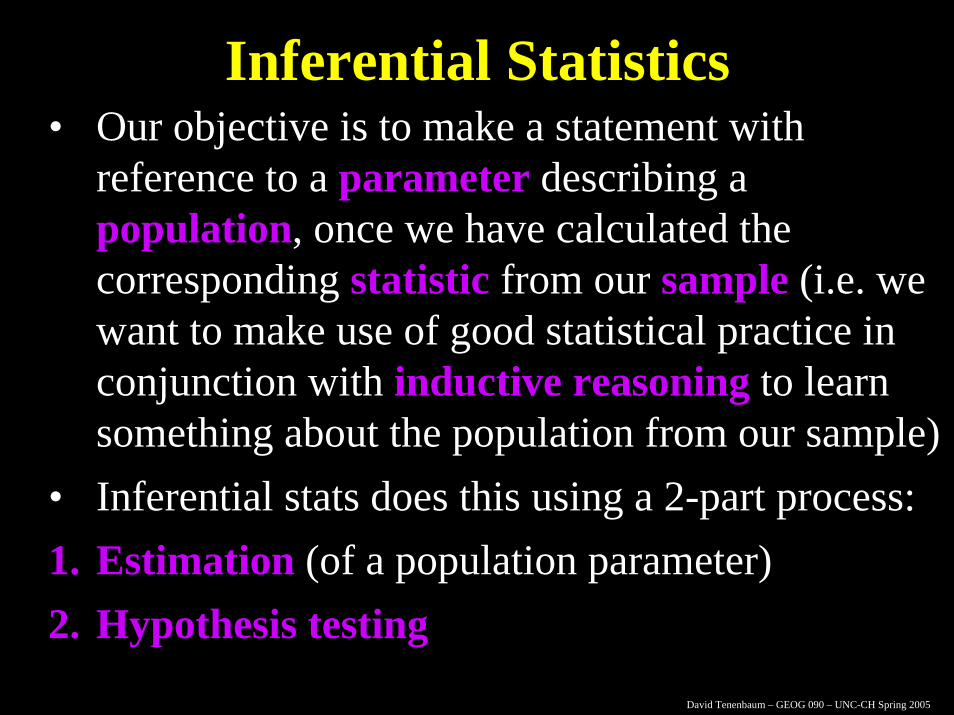
Inferential Statistics• Our objective is to make a statement with

reference to a parameter describing a population, once we have calculated the corresponding statistic from our sample (i.e. we want to make use of good statistical practice in conjunction with inductive reasoning to learn something about the population from our sample)

• Inferential stats does this using a 2-part process:1. Estimation (of a population parameter)2. Hypothesis testing


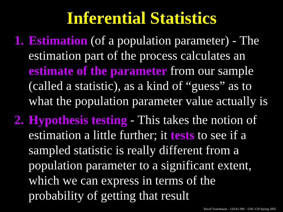
Inferential Statistics1. Estimation (of a population parameter) - The

estimation part of the process calculates an estimate of the parameter from our sample (called a statistic), as a kind of “guess” as to what the population parameter value actually is

2. Hypothesis testing - This takes the notion of estimation a little further; it tests to see if a sampled statistic is really different from a population parameter to a significant extent, which we can express in terms of the probability of getting that result


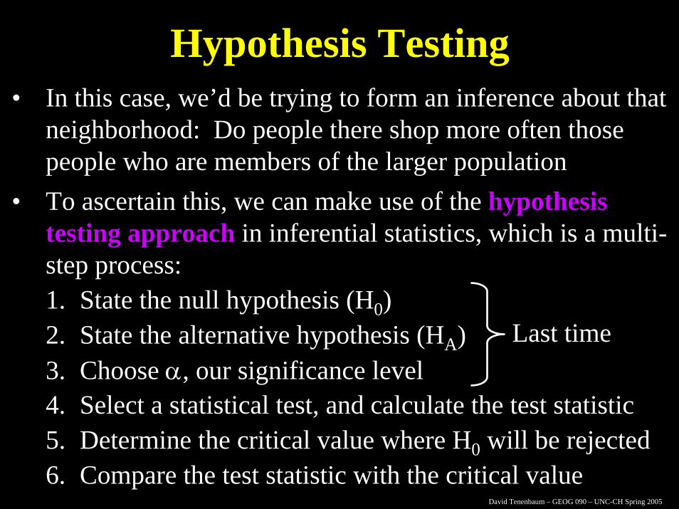
Hypothesis Testing• In this case, we’d be trying to form an inference about that

neighborhood: Do people there shop more often those people who are members of the larger population

• To ascertain this, we can make use of the hypothesis testing approach in inferential statistics, which is a multi-step process:1. State the null hypothesis (H0)2. State the alternative hypothesis (HA)3. Choose α, our significance level4. Select a statistical test, and calculate the test statistic5. Determine the critical value where H0 will be rejected6. Compare the test statistic with the critical value

Last time


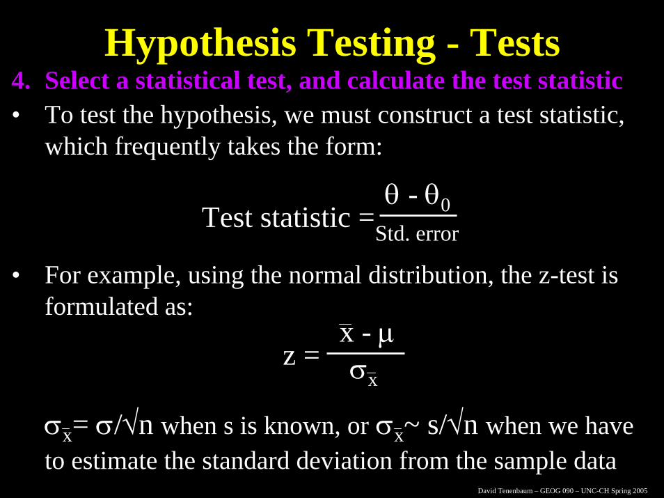
Hypothesis Testing - Tests4. Select a statistical test, and calculate the test statistic• To test the hypothesis, we must construct a test statistic,

which frequently takes the form:

Test statistic =θ - θ0

Std. error

• For example, using the normal distribution, the z-test is formulated as:

z =x - µσx

σx= σ/√n when s is known, or σx~ s/√n when we haveto estimate the standard deviation from the sample data


Hypothesis Testing - Tests4. Select a stat. test, and calculate the test statistic cont.• The Z-test is the ideal test to use when we are comparing

a sample mean to a population mean where the sample is large enough that we can be confident that the sample sampling distribution is normally distributed

• However, in cases where n is smaller (say, n < 30) and we want to compare a sample mean to a population (or two sample means to one another), it is no longer reasonable to assume a normal distribution, so instead we use a test statistic that is based on a similar distribution where the shape of the distribution is related to the sample size

• This family of distributions is known widely as Student’s t distributions, and these are used with a t-test


Hypothesis Testing - Tests4. Select a stat. test, and calculate the test statistic cont.• The Student’s t distribution was invented by William

Gosset, a statistician who worked for the Arthur Guinness and Son brewing company in Dublin, Ireland

• Guinness had a policy that any works invented by its employees could not be published under their own names, thus Gosset was forced to publish his work under the pseudonym ‘Student’

• Gosset invented the t-distribution to solve some practical problems he encountered when trying to enforce quality control in brewing using small samples, and he derived the form of the distribution by a combination of mathematical and empirical work


Hypothesis Testing - Tests4. Select a stat. test, and calculate the test statistic cont.• t-tests are performed in much the same way as Z-tests are,

where a test statistic is calculated and compared to a critical value to see if H0 is accepted or rejected, and we look the critical value up in a different table for a certain α value, but the key difference is that the sample size n is used to calculate the degrees of freedom, which determines the shape of the particular t-distribution to be used, and the critical value (more on this later)

• We can construct confidence intervals around the mean for small samples using t-scores instead of z-scores using more or less the same method, but we would use the t-distribution tables instead of the standard normal tables


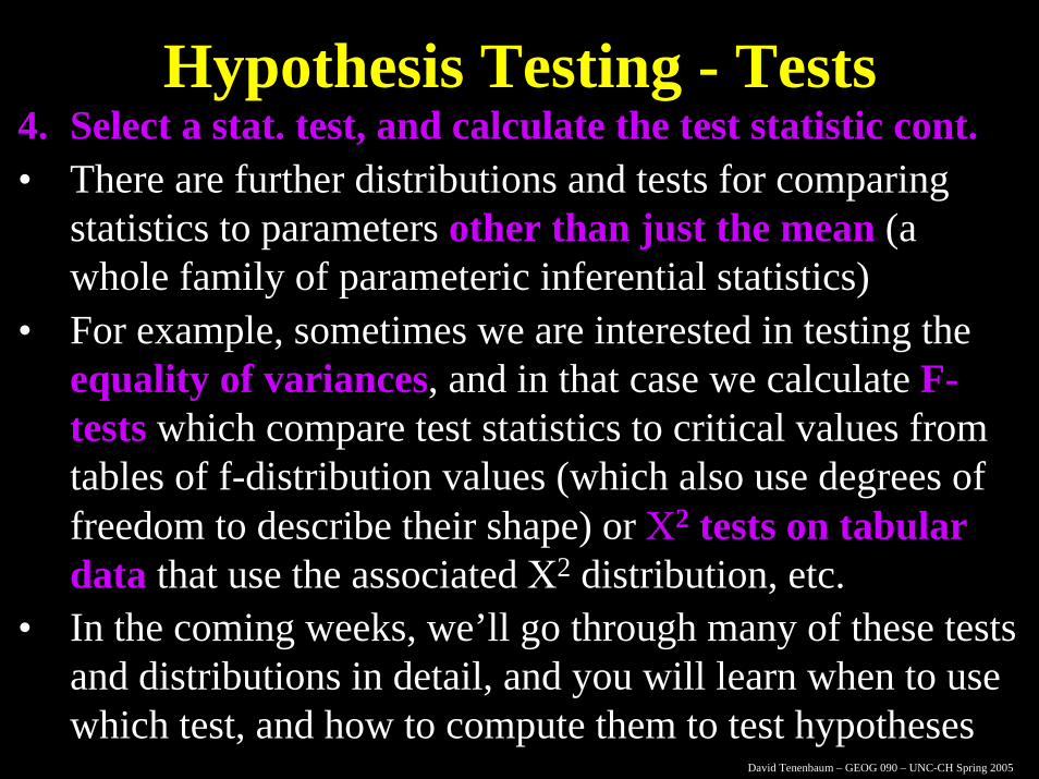
Hypothesis Testing - Tests4. Select a stat. test, and calculate the test statistic cont.• There are further distributions and tests for comparing

statistics to parameters other than just the mean (a whole family of parameteric inferential statistics)

• For example, sometimes we are interested in testing the equality of variances, and in that case we calculate F-tests which compare test statistics to critical values from tables of f-distribution values (which also use degrees of freedom to describe their shape) or Χ2 tests on tabular data that use the associated Χ2 distribution, etc.

• In the coming weeks, we’ll go through many of these tests and distributions in detail, and you will learn when to use which test, and how to compute them to test hypotheses


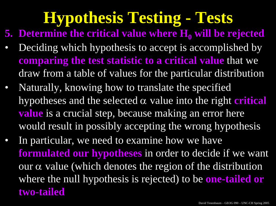
Hypothesis Testing - Tests5. Determine the critical value where H0 will be rejected• Deciding which hypothesis to accept is accomplished by

comparing the test statistic to a critical value that we draw from a table of values for the particular distribution

• Naturally, knowing how to translate the specified hypotheses and the selected α value into the right critical value is a crucial step, because making an error here would result in possibly accepting the wrong hypothesis

• In particular, we need to examine how we have formulated our hypotheses in order to decide if we want our α value (which denotes the region of the distribution where the null hypothesis is rejected) to be one-tailed or two-tailed


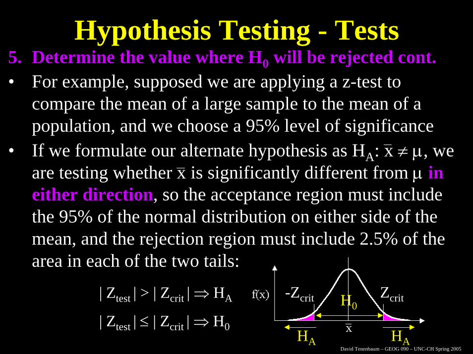
Hypothesis Testing - Tests5. Determine the value where H0 will be rejected cont.• For example, supposed we are applying a z-test to

compare the mean of a large sample to the mean of a population, and we choose a 95% level of significance

• If we formulate our alternate hypothesis as HA: x ≠ µ, we are testing whether x is significantly different from µ in either direction, so the acceptance region must include the 95% of the normal distribution on either side of the mean, and the rejection region must include 2.5% of the area in each of the two tails:

| Ztest | > | Zcrit | ⇒ HA

| Ztest | ≤ | Zcrit | ⇒ H0

Zcrit-Zcrit H0

HA HA


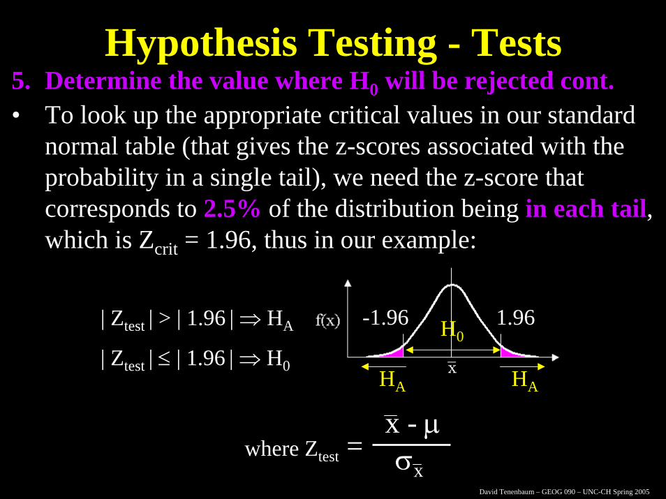
Hypothesis Testing - Tests5. Determine the value where H0 will be rejected cont.• To look up the appropriate critical values in our standard

normal table (that gives the z-scores associated with the probability in a single tail), we need the z-score that corresponds to 2.5% of the distribution being in each tail, which is Zcrit = 1.96, thus in our example:

| Ztest | > | 1.96 | ⇒ HA

| Ztest | ≤ | 1.96 | ⇒ H0

1.96-1.96 H0

HA HA

where Ztest =x - µσx


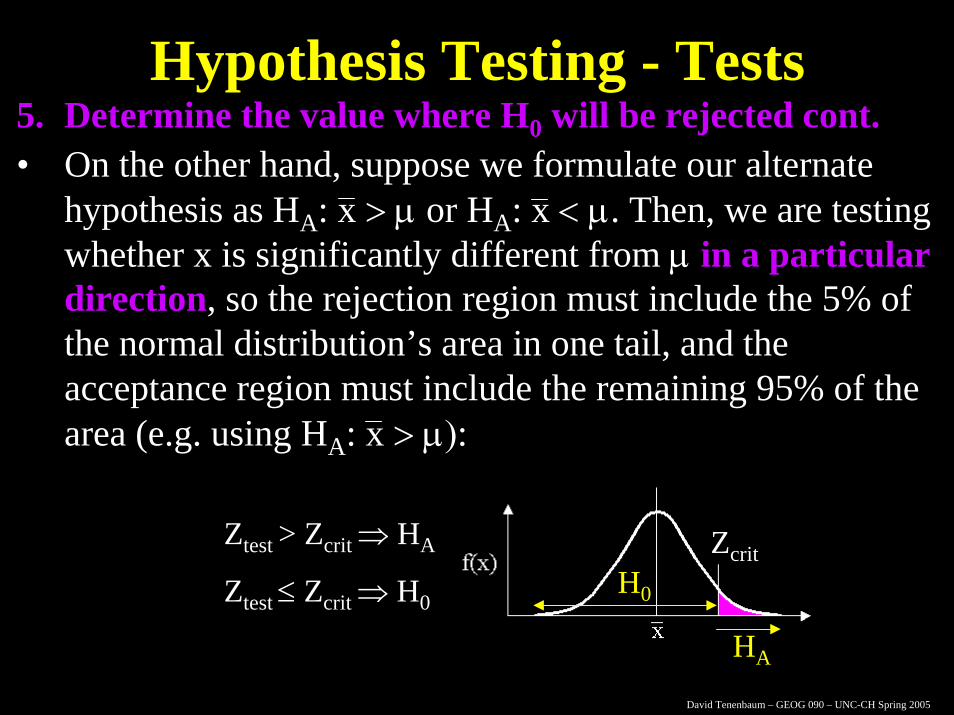
Hypothesis Testing - Tests5. Determine the value where H0 will be rejected cont.• On the other hand, suppose we formulate our alternate

hypothesis as HA: x > µ or HA: x < µ. Then, we are testing whether x is significantly different from µ in a particular direction, so the rejection region must include the 5% of the normal distribution’s area in one tail, and the acceptance region must include the remaining 95% of the area (e.g. using HA: x > µ):

Ztest > Zcrit ⇒ HA

Ztest ≤ Zcrit ⇒ H0

ZcritH0

HA


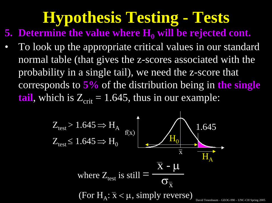
Hypothesis Testing - Tests5. Determine the value where H0 will be rejected cont.• To look up the appropriate critical values in our standard

normal table (that gives the z-scores associated with the probability in a single tail), we need the z-score that corresponds to 5% of the distribution being in the single tail, which is Zcrit = 1.645, thus in our example:

where Ztest is still =x - µσx

Ztest > 1.645 ⇒ HA

Ztest ≤ 1.645 ⇒ H0

1.645H0

HA

(For HA: x < µ, simply reverse)


Hypothesis Testing - Tests5. Determine the value where H0 will be rejected cont.• We can make use of some previous knowledge of how we

think a sample is positioned compared to the population when we formulate our hypotheses in order to use an appropriate one-tailed test, because when using two-tailed tests it is even more difficult to reject the null hypothesis (since you need an even greater | z-score | to surpass the zcrit than you would with a one-tailed test) as compared to the more sensitive one-tailed test

6. Compare the test statistic with the critical value• Now that we have our test statistic our critical value, we

compare the values and determine which hypothesis to accept


Hypothesis Testing - Example• Remember the poll we theoretically conducted to

try and get a sense of the outcome of an upcoming election with two candidates? We polled 1000 people, and 550 of them responded that they would vote for Candidate A.

• Suppose we now have the results of the election, including a the proportion of the popular vote that Candidate A received (52%), and we want to check and see if the sample we took in our poll reflected a candidate preference that was significantly different from how the population as a whole decided to vote


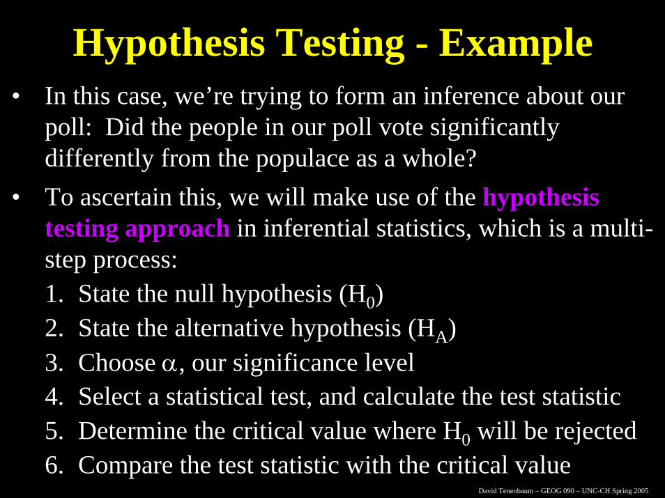
Hypothesis Testing - Example• In this case, we’re trying to form an inference about our

poll: Did the people in our poll vote significantly differently from the populace as a whole?

• To ascertain this, we will make use of the hypothesis testing approach in inferential statistics, which is a multi-step process:1. State the null hypothesis (H0)2. State the alternative hypothesis (HA)3. Choose α, our significance level4. Select a statistical test, and calculate the test statistic5. Determine the critical value where H0 will be rejected6. Compare the test statistic with the critical value


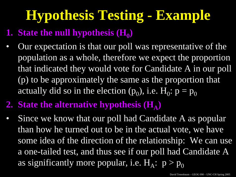
Hypothesis Testing - Example1. State the null hypothesis (H0)• Our expectation is that our poll was representative of the

population as a whole, therefore we expect the proportion that indicated they would vote for Candidate A in our poll (p) to be approximately the same as the proportion that actually did so in the election (p0), i.e. H0: p = p0

2. State the alternative hypothesis (HA)• Since we know that our poll had Candidate A as popular

than how he turned out to be in the actual vote, we have some idea of the direction of the relationship: We can use a one-tailed test, and thus see if our poll had Candidate A as significantly more popular, i.e. HA: p > p0


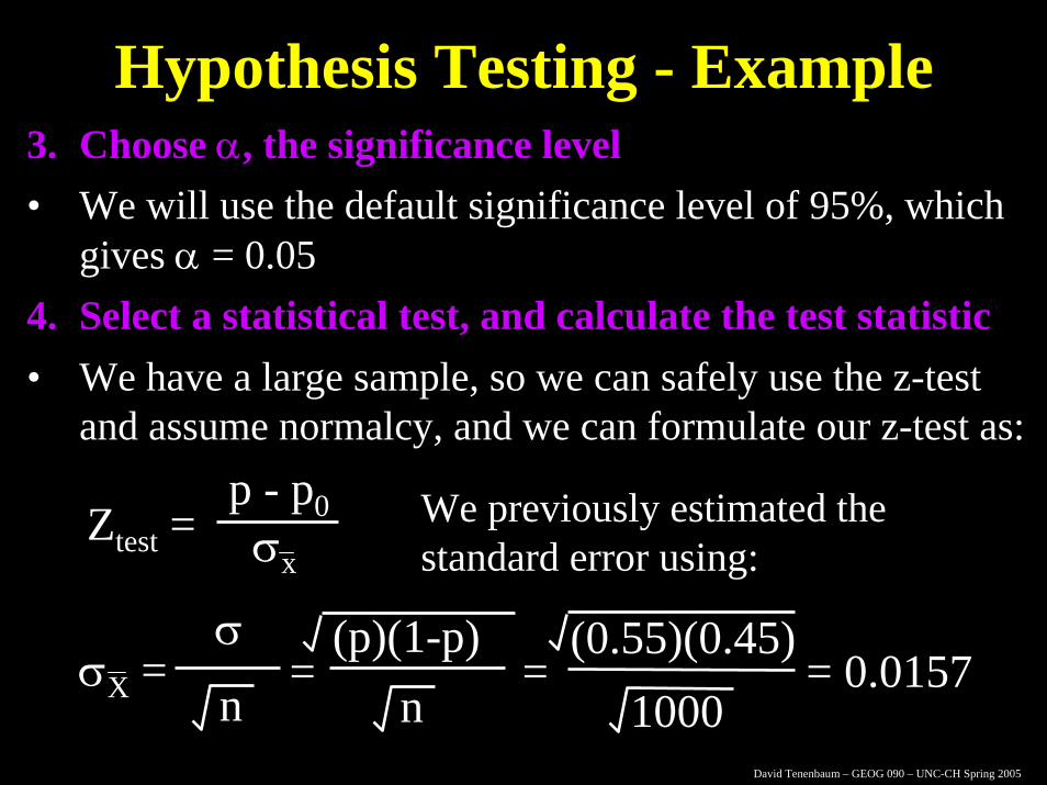
Hypothesis Testing - Example3. Choose α, the significance level• We will use the default significance level of 95%, which

gives α = 0.054. Select a statistical test, and calculate the test statistic• We have a large sample, so we can safely use the z-test

and assume normalcy, and we can formulate our z-test as:p - p0Ztest = σx

σX =σ

n=

(p)(1-p)n

=(0.55)(0.45)

1000= 0.0157

We previously estimated the standard error using:


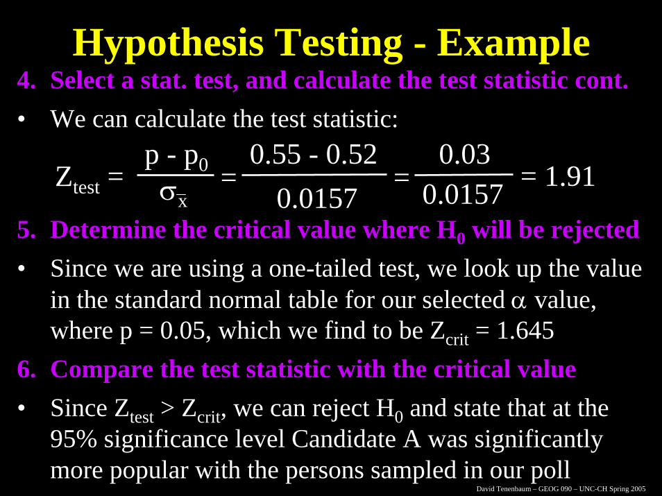
Hypothesis Testing - Example4. Select a stat. test, and calculate the test statistic cont.• We can calculate the test statistic:

p - p0Ztest = σx=

0.55 - 0.520.0157

=0.03

0.0157 = 1.91

5. Determine the critical value where H0 will be rejected• Since we are using a one-tailed test, we look up the value

in the standard normal table for our selected α value, where p = 0.05, which we find to be Zcrit = 1.645

6. Compare the test statistic with the critical value• Since Ztest > Zcrit, we can reject H0 and state that at the

95% significance level Candidate A was significantly more popular with the persons sampled in our poll


Hypothesis Testing - Example6. Compare the test statistic with the critical value cont.• Note that had we stated our alternate hypothesis

differently (i.e. is there a significant difference between the poll and the election result) and not stated the direction of the difference, and thus chosen to use a two-tailed test at the 95% significance level, the resulting Zcritwould have been 1.96

• Since our calculated Ztest value was 1.91, we would have failed to reject the null hypothesis for a two-tailed alternate hypothesis, and would have concluded that the poll and election result depicted Candidate A’s popularity in a fashion that was not significantly different!


An Alternative to Hypothesis Testing• Because the selection of a particular level of significance

is a somewhat arbitrary decision, we can potentially prove any hypothesis by adjusting α accordingly

• As an alternative, we can take the probability value approach, which gives a sense of the degree of belief we have in our conclusion by reporting the probability that we have incorrectly rejected the null hypothesis, e.g. using our Ztest of 1.91, we find the probability in the standard normal table for that value to be α = 0.0281, therefore we can state that there is a 97.19% level of probability that we have correctly rejected the null hypothesis and stated that those that we polled preferred Candidate A significantly over the whole of the voting population

Documents

Inferential Statistics · David Tenenbaum – GEOG 090 – UNC-CH Spring 2005 Inferential Statistics • Our objective is to make a statement with reference to a parameter describing