Inference Remapping for Vehicular Analytics

Paramvir Bahl Srikanth Kandula Ashish Patro Mohammed ShoaibMicrosoft Research, Redmond WA 98052

Abstract– A phone+car+cloud system can improve manyvehicular scenarios significantly due to improved telemetryand the resulting optimizations. The core problem howeveris the inability to cope when inputs are missing or impossi-ble to obtain apriori. We develop the concept of inferenceremapping which learns using correlations how to best useavailable substitutes for the missing inputs. We also describean end-to-end system Sparc that combines an OBD device, aphone app and a cloud backend to drive a variety of applica-tions. In particular, for the case of fuel usage prediction, weobtain a mechanical engineering theory based model that isaccurate to within 2% when given ideal inputs (OBD data).We show how to remap the inference to only use phone data(7% error) or data available from a map (within 20% errorfor half the rides, which is 4× more accurate than state-of-art). A side-effect of our model is that we can offer detailedcomparative feedback to drivers on their driving behavior.

1. INTRODUCTIONWe have to transform how we use automobiles to reduceurban gridlock, pollution, and our impact on the climate.Connecting vehicles to the cloud offers improved teleme-try and can lead to optimizations that lower cost, both indi-vidual and societal, and improve user experience. A recentstudy [22] finds that 11-13% of commute time is due to traf-fic congestion, 10-17% of urban fuel is wasted at stoplightswhere there is no cross traffic, and 80% of accidents are dueto driver distraction. A cloud-connected car can be routedalong the least congested path, directed to an available park-ing space and can offer rich feedback on driving behaviorand vehicle’s condition.

We would like to offer value in four different contexts:Before driving: E.g., Does my car have enough gas after mydaughter/son drove it last night? What route should I take tosave fuel/ save time? Is my car in good running condition?While driving: E.g., Where will I quickly find parking? Im-pending congestion or accidents along the forward route? Iam running late, is my contact aware of my estimated timeof arrival? After driving: E.g., How much did that trip cost?How could I have driven better? How do I compare to otherdrivers? When not driving: E.g., Is my child/mother drivingsafely? Where is my spouse? Is it safe to text him/her now?

Smartphones are a key enabler here. In part, because theyhave sensors and a backhaul to the cloud that cars may nototherwise have. More fundamentally however, phone soft-ware and hardware can update much more quickly relative

to the average lifetime of a car (averages 17 years [22]) al-lowing for rapid innovation. Further, it has become rela-tively easy to interface with the car. Bluetooth devices thatplug into the on-board diagnostics (OBD) port or speak thecar-area-network bus (CANBUS) protocol are available atlow cost. These devices can monitor detailed vehicle statesuch as the instantaneous rate of fuel being injected into theengine. As a result, we note a recent substantial increasein startup activity in vehicular phone apps– some improvedriver risk profiling for insurance [10, 23] and others offertrip analytics and assist with parking [24, 6].

We argue that a commonly recurring problem here is theinability to cope with missing inputs. For e.g., Automatic [6]infers how much fuel was spent on each segment after a ride.But, it cannot do so if the OBD device is not installed orif the phone app loses connectivity with the OBD device.Anecdotal evidence from our deployment reveals that this isby far the common case. Relatively few drivers install ad-ditional devices and even for those that do, the OBD feed isnot always available for mundane reasons such as the driverbumping device with her leg or due to hardware and softwarefaults on the OBD device.

Worse, in some cases, the inferences are needed before theinputs are available. For e.g., picking the most fuel-efficientroute requires predicting how much fuel will be spent bya car along each potential route. But, how can we do thiswithout the sensor feed from OBD for each route?

We call this the inference remapping problem. That is,suppose an inference algorithm requires some inputs and of-fers an output. Can we adapt the algorithm to work whensome of these inputs are missing or are impossible to obtain(as they are for the case of predictions)? If solvable, this sub-stantially increases the coverage of any inference technique–inferences may be available for {cars, drivers, routes, times}for which no sensor feed exists. Continuing our fuel usageexample, with remapping, one could infer the fuel use fora car, driver, route and (future) time without the driver in-stalling an OBD device or driving that car along that route.

Our basic intuition is simple: substitute the missing in-puts with similar data that is available. For e.g., the speedlimits, slopes or road segments and location of stop lightsare available from a map. Could we estimate the absentOBD feed from such roadstate information? In some cases,other drivers or other cars may have driven along a route.Can we extrapolate from one driver or car to another? Also,the phone sensor information can partially substitute for the

1

OBD feed. Can we estimate what the OBD feed would havebeen from a phone sensor feed?

The key challenge however is that to get a high qualityinference with these substitute inputs, one has to carefullycapture the aspects of the ideal inputs that matter for theinference and identify how to estimate them from the sub-stitute inputs. For e.g., we will show later that estimatingfuel use on a road depends significantly on how the speedchanges when driving on that road. The energy efficiencyof an engine varies with the speed. Sharp speed increasesrequire more energy than gradual increases. Decreases inspeed due to braking mostly dissipate as heat so while theaverage speed of two rides may be the same, the ride withmore changes in speed uses more fuel. There is also a com-plex dependence with the road slope and vehicular charac-teristics such as mass and frontal area. When going down ahill how much of the lost potential energy translates to speedincrease depends on the aerodynamics of the vehicle. An-other challenge is that the substitute inputs fundamentallylack some aspects of the ideal input. For e.g., OBD feeds re-veal the torque generated by the engine. None of the phonesensors match directly to engine torque. More details followlater; but in short, transforming substitute inputs to mimicthe ideal inputs is non-trivial.

In this paper, we present the Sparc system 1 that takes afirst step towards solving the inference remapping problem.For the example fuel usage inference, Sparc uses mechani-cal engineering theory to build a model of vehicular energyusage. For the case when ideal inputs are available fromthe OBD device, Sparc learns the parameter inputs for thismodel using regression from just a small amount of OBDdata. Sparc also shows how to remap the inference to useinputs from just the phone sensors or just the informationavailable from a map. The latter allows Sparc to predict fuelusage on a route even when Sparc has no drive-feed be itfrom a phone or OBD device for that route.

Further, we built Sparc end-to-end and offer results froma deployment study on twenty cars in two cities over sixmonths. Sparc has an extensible data-collection platform,comprising a mobile app and a cloud-server backend. Theapp collects data from phone sensors and an OBD devicein the car over Bluetooth. It has an asynchronous data-management framework leading to power-efficient data up-loads without user intervention. Sparc map-matches GPSreadings to acquire road grade and traffic information [18,26]. We use data from OpenStreetMaps as well as a propri-etary vendor. Finally, besides collecting telemetry informa-tion for data insights, Sparc also communicates to the cloudin real-time allowing it to enable the use-cases described inthe second paragraph.

A side-effect of the remapping model used for fuel usageestimation is the ability to provide a precise breakdown ofwhere fuel is spent. For e.g., Sparc breaks down the energyspent into the parts required to combat aerodynamic drag,

1Sparc = Smartphone + Car + Cloud

increase kinetic energy, increase potential energy, to combatrolling resistance etc. This breakdown helps answer ques-tions such as: how does cruise control impact fuel use? Fur-ther, by comparing drivers traversing similar roads, we offercomparative feedback on driving styles such as accelerationand braking patterns and the impact of driving styles and carchoice on fuel usage.

Our key contributions are:

• An extensible end-to-end smartphone+car+cloud sys-tem that collects telemetry data and offers various ap-plications to drivers (§3).

• A first solution to the inference remapping problem forthe case of fuel usage prediction (§2). The ideal in-puts from OBD device yield a 2% error indicating thatthe mechanical-engineering based model is reasonablycomplete. We show that using just the phone sensors,the fuel estimation error is below 7% (§5.2). Further,when predicting fuel use on roads for which it has nodriving feed, Sparc is roughly 4× more accurate rela-tive to the state-of-art: 48% of trips are predicted towithin 20% error (§5.3).

• Results for driver feedback and comparative analysis(§5.4) on a sizable longitudinal study identifies driverswith under-inflated tires (more rolling resistance thanexpected), a sedan driver with such gradual brakingpattern that he reclaims more of the kinetic energy thatwould otherwise be lost than a hybrid SUV and driverswhose dominant energy loss is aerodynamic drag (highfrontal area predominantly driven on highways at verylarge speeds).

We note however that the ability to remap inferences de-pends both on the property being inferred and the quality ofthe substitute input. For e.g., anomalies such as hard brak-ing instances can be estimated using OBD feed; accelerom-eter readings from the phone can substitute but roadstateinformation would not suffice. Further, inference remap-ping is similar to techniques like PCA that leverage cor-relation between disjoint datastreams. However, whereassuch work [25] saves energy by monitoring and communi-cating only the subset of inputs that is most useful for infer-ence, here, we focus on obtaining the best possible inferencegiven whichever subset of inputs and substitutes happen tobe available. More specifically, the problem at hand – fuelusage prediction – is complex function rooted in the physi-cal world. This leads to positives (can leverage mechanicalengineering theory) and challenges (many factors affect fuelin intricate ways). Finally, GreenGPS [16] was the first totackle the problem of fuel usage estimation. Sparc newlyoffers driving feedback and develops inference remapping.The major change is a much more detailed modeling of en-ergy use and remapping. Without either the estimation errorswere substantial on our dataset perhaps because it containsrides from urban settings with very different congestion pro-files and a variety of road slopes. Our dataset lacks data

2

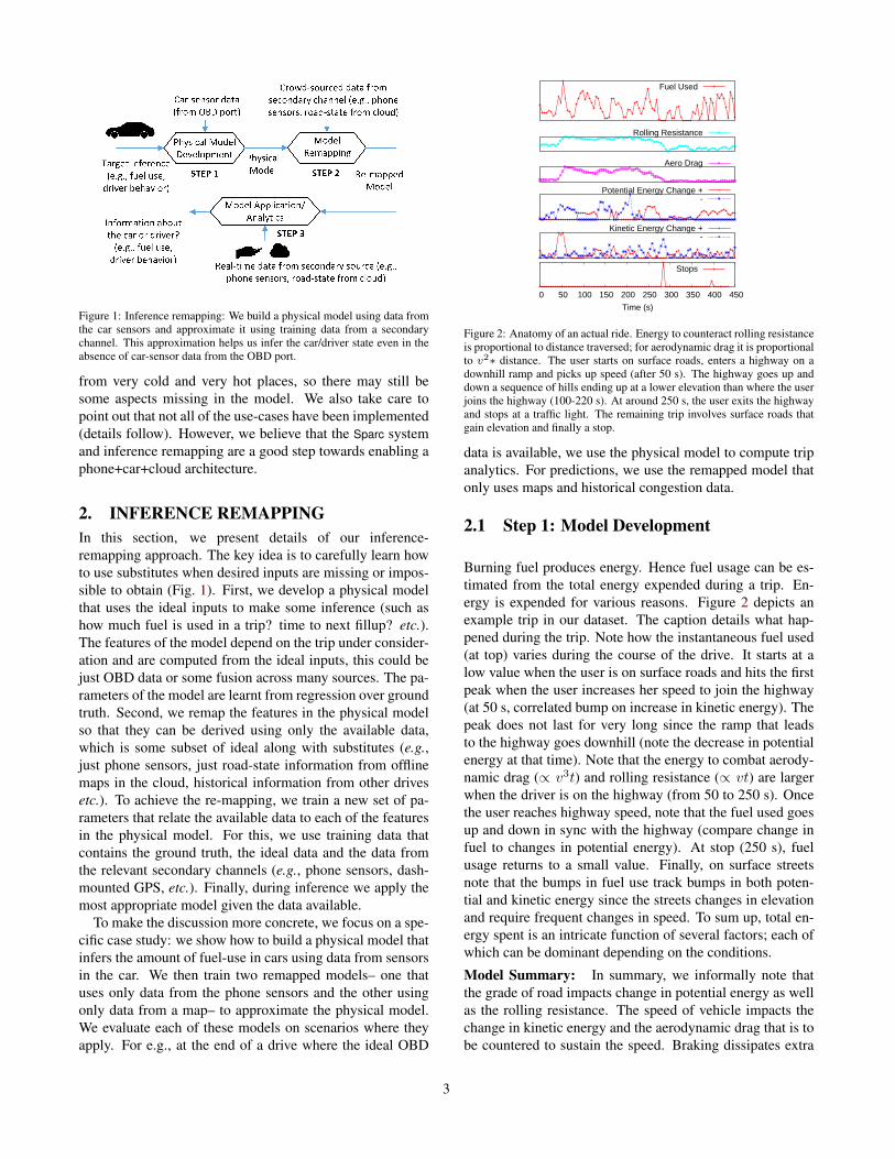
Figure 1: Inference remapping: We build a physical model using data fromthe car sensors and approximate it using training data from a secondarychannel. This approximation helps us infer the car/driver state even in theabsence of car-sensor data from the OBD port.

from very cold and very hot places, so there may still besome aspects missing in the model. We also take care topoint out that not all of the use-cases have been implemented(details follow). However, we believe that the Sparc systemand inference remapping are a good step towards enabling aphone+car+cloud architecture.

2. INFERENCE REMAPPINGIn this section, we present details of our inference-remapping approach. The key idea is to carefully learn howto use substitutes when desired inputs are missing or impos-sible to obtain (Fig. 1). First, we develop a physical modelthat uses the ideal inputs to make some inference (such ashow much fuel is used in a trip? time to next fillup? etc.).The features of the model depend on the trip under consider-ation and are computed from the ideal inputs, this could bejust OBD data or some fusion across many sources. The pa-rameters of the model are learnt from regression over groundtruth. Second, we remap the features in the physical modelso that they can be derived using only the available data,which is some subset of ideal along with substitutes (e.g.,just phone sensors, just road-state information from offlinemaps in the cloud, historical information from other drivesetc.). To achieve the re-mapping, we train a new set of pa-rameters that relate the available data to each of the featuresin the physical model. For this, we use training data thatcontains the ground truth, the ideal data and the data fromthe relevant secondary channels (e.g., phone sensors, dash-mounted GPS, etc.). Finally, during inference we apply themost appropriate model given the data available.

To make the discussion more concrete, we focus on a spe-cific case study: we show how to build a physical model thatinfers the amount of fuel-use in cars using data from sensorsin the car. We then train two remapped models– one thatuses only data from the phone sensors and the other usingonly data from a map– to approximate the physical model.We evaluate each of these models on scenarios where theyapply. For e.g., at the end of a drive where the ideal OBD

0 50 100 150 200 250 300 350 400 450

Time (s)

Stops

Kinetic Energy Change +-

Potential Energy Change +-

Aero Drag

Rolling Resistance

Fuel Used

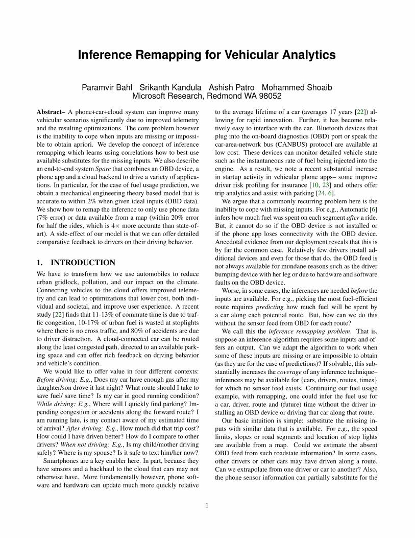
Figure 2: Anatomy of an actual ride. Energy to counteract rolling resistanceis proportional to distance traversed; for aerodynamic drag it is proportionalto v2∗ distance. The user starts on surface roads, enters a highway on adownhill ramp and picks up speed (after 50 s). The highway goes up anddown a sequence of hills ending up at a lower elevation than where the userjoins the highway (100-220 s). At around 250 s, the user exits the highwayand stops at a traffic light. The remaining trip involves surface roads thatgain elevation and finally a stop.

data is available, we use the physical model to compute tripanalytics. For predictions, we use the remapped model thatonly uses maps and historical congestion data.

2.1 Step 1: Model Development

Burning fuel produces energy. Hence fuel usage can be es-timated from the total energy expended during a trip. En-ergy is expended for various reasons. Figure 2 depicts anexample trip in our dataset. The caption details what hap-pened during the trip. Note how the instantaneous fuel used(at top) varies during the course of the drive. It starts at alow value when the user is on surface roads and hits the firstpeak when the user increases her speed to join the highway(at 50 s, correlated bump on increase in kinetic energy). Thepeak does not last for very long since the ramp that leadsto the highway goes downhill (note the decrease in potentialenergy at that time). Note that the energy to combat aerody-namic drag (∝ v3t) and rolling resistance (∝ vt) are largerwhen the driver is on the highway (from 50 to 250 s). Oncethe user reaches highway speed, note that the fuel used goesup and down in sync with the highway (compare change infuel to changes in potential energy). At stop (250 s), fuelusage returns to a small value. Finally, on surface streetsnote that the bumps in fuel use track bumps in both poten-tial and kinetic energy since the streets changes in elevationand require frequent changes in speed. To sum up, total en-ergy spent is an intricate function of several factors; each ofwhich can be dominant depending on the conditions.

Model Summary: In summary, we informally note thatthe grade of road impacts change in potential energy as wellas the rolling resistance. The speed of vehicle impacts thechange in kinetic energy and the aerodynamic drag that is tobe countered to sustain the speed. Braking dissipates extra

3

kinetic energy into heat. Vehicle-specific parameters suchas the mass impact both potential and kinetic-energy terms.The vehicles’ aerodynamicity affects drag. The engine anddrivetrain efficiency impact how much useful energy is gen-erated from burning fuel. Driver-specific behavior such ashard acceleration, braking, and transmission shifts also im-pact energy use: when accelerating hard, the vehicle’s fuelinjection unit has less time to modulate fuel injected leadingto less useful energy for the same fuel burnt. Finally, mis-cellaneous aspects include windows being open, the temper-ature, use of A/C and other electrical equipment. The de-tailed model follows.

Model Details: To develop an instantaneous model of en-ergy consumption from first principles, consider a small pe-riod of time ∆t. Suppose that the vehicle moves with veloc-ity v on a road of grade θ, changes velocity by ∆v , and burnsfuel at a rate f .

(instantaneous) Energy generated by the engine = ηf∆t

where η, usually termed engine specific fuel consumption,indicates the engine’s efficiency in burning fuel; this is afunction of torque and engine revolutions-per-minute (RPM)[8]. Slower speeds (low RPM) and/or very high torque val-ues lead to lower η values. However, most engines havea large operating region where the engine’s efficiency isroughly the same. Typical combustion engines have an effi-ciency around 30%; i.e., roughly 30% of the heat producedby burning fuel is converted into mechanical energy.

(instantaneous) Mechanical energy at engine = τω∆t

where τ is the torque and ω is the RPM at the engine. Thisenergy is used in a few ways. The (Instantaneous) energyspent can be attributed to the various reasons shown in Ta-ble 1. Note that some of the energy losses can be used tooffset other needs. For instance, one can slow down with-out braking, by letting loss in kinetic energy compensate forrolling resistance and aero drag. While every increase in po-tential or kinetic energy requires burning fuel, their loss isnot fully recovered. For example, most braking dissipateskinetic energy into heat. Thus, we assume some recoveryfactors (R1, R2) and treat the changes differently based onwhether they are increases or decreases.

By the law of conservation of energy, we have:

Energy generated + Recovered = Energy used.

Using all of the energy components show in Table 1 and re-

arranging terms, we have:

ηf∆t = τω∆t

= Pe∆t + PsIs∆t

+mg[sinθ]0+v∆t +mv[∆v]0+

ηt

+crrmgcosθv∆t + 1

2cd A ρv3∆t

ηt

+R1mg[sin θ]0− v∆t +R2mv [∆v]0− . (1)

2.1.1 Features of a TripObserve that the physical energy-consumption model inEquation 1 relates fuel use (on the left) to measurable as-pects of the trip (on the right). We will call the measurableaspects of a trip to be the features of that trip. Table 2 listsour current set of features. How to estimate these features inthe ideal case? A device plugged into the OBD port of thecar can report these sensor readings: f , v, ω, and τ , whichrepresent the mass air flow sensor output (i.e., the fuel in-jection rate), vehicular speed, RPM, and torque as measuredby the vehicle’s engine control unit. Phone’s GPS provideslocation, which when map-matched can reveal the slope ofeach road segment θ. The data is usually sampled once everyfew seconds at each of these sources but needs to be fusedproperly (more details in §2.2.1).

Note that the values in the right column of Table 2 are amultiplicative parameter away from the corresponding en-ergy term on the left in the vehicular energy model (Equa-tion 1). These parameters m, A, and η, stand for the mass ofthe car, its effective area and the engine’s efficiency, whichis itself a function of torque and RPM. These coefficients arespecific to a car and can vary from one trip to the other.

Given trip features and the fuel usage ground-truth in-formation from OBD, we pursued a few approaches tolearn car-specific multiplicative parameters: (a) linear re-gression with the above features, (b) non-linear regressionwith the underlying raw variables such as velocity, timeand slope (v, t, θ), (c) a classifier that uses discretized “fu-elUsage" as the label (e.g., [0-.1) gallons, [.1-.2), ...) and(d) decision trees. Linear regression worked the best whenused in the following way: (1) 10-fold cross-validation toavoid overfitting, (2) to keep the parameters robust to tripduration, combine features from contiguous epochs so as toeffectively train on epochs of many different sizes.

Why does linear regression do well? Because, at firstblush the features are not even independent (see Table 2),so shouldn’t linear regression be a bad choice? We foundthat using the underlying variables (e.g, v, θ) as features re-quires learning a non-linear model for which known algo-rithms are less effective. Decision trees or a classifier withfuelUsage would have been better if the epochs were divis-ible into regimes where the relationship between fuel usageand the trip features differs substantially. Decision trees didobtain slightly lower error, however the trees were much big-ger, hinting at potential overfitting.

4

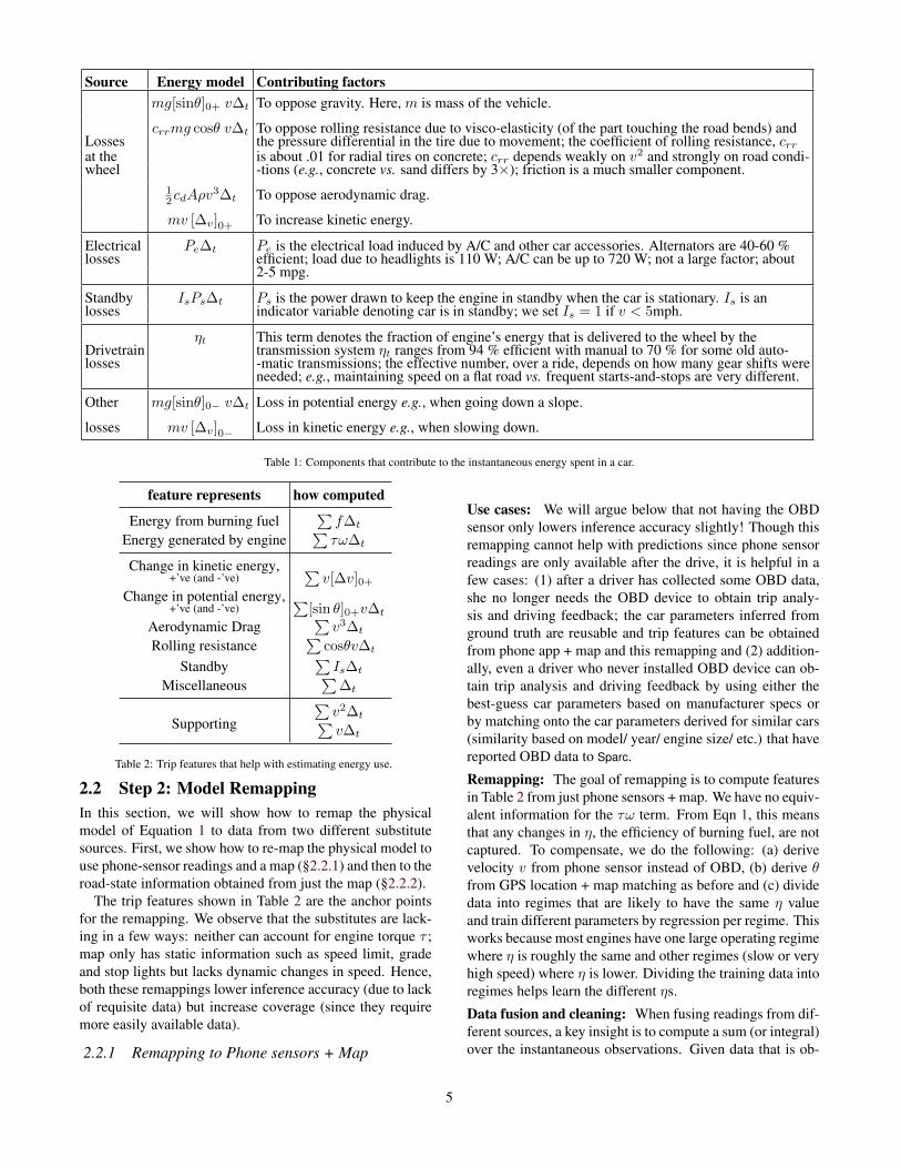
Source Energy model Contributing factorsmg[sinθ]0+ v∆t To oppose gravity. Here, m is mass of the vehicle.

crrmg cosθ v∆t To oppose rolling resistance due to visco-elasticity (of the part touching the road bends) andLosses the pressure differential in the tire due to movement; the coefficient of rolling resistance, crrat the is about .01 for radial tires on concrete; crr depends weakly on v2 and strongly on road condi-wheel -tions (e.g., concrete vs. sand differs by 3×); friction is a much smaller component.

12cdAρv

3∆t To oppose aerodynamic drag.

mv [∆v]0+ To increase kinetic energy.

Electrical Pe∆t Pe is the electrical load induced by A/C and other car accessories. Alternators are 40-60 %losses efficient; load due to headlights is 110 W; A/C can be up to 720 W; not a large factor; about

2-5 mpg.

Standby IsPs∆t Ps is the power drawn to keep the engine in standby when the car is stationary. Is is anlosses indicator variable denoting car is in standby; we set Is = 1 if v < 5mph.

ηt This term denotes the fraction of engine’s energy that is delivered to the wheel by theDrivetrain transmission system ηt ranges from 94 % efficient with manual to 70 % for some old auto-losses -matic transmissions; the effective number, over a ride, depends on how many gear shifts were

needed; e.g., maintaining speed on a flat road vs. frequent starts-and-stops are very different.

Other mg[sinθ]0− v∆t Loss in potential energy e.g., when going down a slope.

losses mv [∆v]0− Loss in kinetic energy e.g., when slowing down.

Table 1: Components that contribute to the instantaneous energy spent in a car.

feature represents how computed

Energy from burning fuel∑f∆t

Energy generated by engine∑τω∆t

Change in kinetic energy, ∑v[∆v]0++’ve (and -’ve)

Change in potential energy, ∑[sin θ]0+v∆t+’ve (and -’ve)

Aerodynamic Drag∑v3∆t

Rolling resistance∑

cosθv∆t

Standby∑Is∆t

Miscellaneous∑

∆t

Supporting

∑v2∆t∑v∆t

Table 2: Trip features that help with estimating energy use.

2.2 Step 2: Model RemappingIn this section, we will show how to remap the physicalmodel of Equation 1 to data from two different substitutesources. First, we show how to re-map the physical model touse phone-sensor readings and a map (§2.2.1) and then to theroad-state information obtained from just the map (§2.2.2).

The trip features shown in Table 2 are the anchor pointsfor the remapping. We observe that the substitutes are lack-ing in a few ways: neither can account for engine torque τ ;map only has static information such as speed limit, gradeand stop lights but lacks dynamic changes in speed. Hence,both these remappings lower inference accuracy (due to lackof requisite data) but increase coverage (since they requiremore easily available data).

2.2.1 Remapping to Phone sensors + Map

Use cases: We will argue below that not having the OBDsensor only lowers inference accuracy slightly! Though thisremapping cannot help with predictions since phone sensorreadings are only available after the drive, it is helpful in afew cases: (1) after a driver has collected some OBD data,she no longer needs the OBD device to obtain trip analy-sis and driving feedback; the car parameters inferred fromground truth are reusable and trip features can be obtainedfrom phone app + map and this remapping and (2) addition-ally, even a driver who never installed OBD device can ob-tain trip analysis and driving feedback by using either thebest-guess car parameters based on manufacturer specs orby matching onto the car parameters derived for similar cars(similarity based on model/ year/ engine size/ etc.) that havereported OBD data to Sparc.

Remapping: The goal of remapping is to compute featuresin Table 2 from just phone sensors + map. We have no equiv-alent information for the τω term. From Eqn 1, this meansthat any changes in η, the efficiency of burning fuel, are notcaptured. To compensate, we do the following: (a) derivevelocity v from phone sensor instead of OBD, (b) derive θfrom GPS location + map matching as before and (c) dividedata into regimes that are likely to have the same η valueand train different parameters by regression per regime. Thisworks because most engines have one large operating regimewhere η is roughly the same and other regimes (slow or veryhigh speed) where η is lower. Dividing the training data intoregimes helps learn the different ηs.

Data fusion and cleaning: When fusing readings from dif-ferent sources, a key insight is to compute a sum (or integral)over the instantaneous observations. Given data that is ob-

5

0

20

40

60

80

100Speed (

mph)

Road Segment, sorted by posted speed limit

Obs. SpeedPosted limit

0

5

10

15

20

25

30

0 10 20 30 40 50 60 70

Std

ev o

f Speed (

mph)

Avg. Speed on Road Segment (mph)

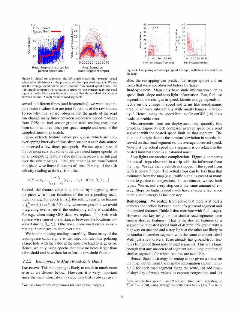
Figure 3: Speed on segments: the left graph shows the (average) speedachieved by all drivers vs. the posted speed limit per road segment. We seethat the average speed can be quite different from posted speed limits. Theright graph compares the variation in speed vs. the average again per roadsegment. Solid blue plots the trend; we see that the standard deviation isbetween 10 and 15 mph for most road segments.

served at different times (and frequencies), we want to com-pute feature values that are joint functions of the raw values.To see why this is hard, observe that the grade of the roadcan change many times between successive speed readingsfrom GPS; the fuel sensor ground truth reading may havebeen sampled three times per speed sample and none of thesampled times may match.

Sparc extracts feature values per epochs which are non-overlapping intervals of time sized such that each data sourceis observed a few times per epoch. We use epoch size of5 s for most cars but some older cars need larger epochs of60 s. Computing feature value mimics a piece-wise integralover the raw readings. First, the readings are transformedinto piece-wise linear functions of time. For e.g., if the i’thvelocity reading at time ti is vi, then

v(t) = vi +t− ti

ti+1 − ti(vi+1 − vi) if t ∈ [ti, ti+1].

Second, the feature value is computed by integrating overthe piece-wise linear functions of the corresponding read-ings. For e.g., for epoch [tb, te], the rolling resistance featureis∫ tetbcosθ(t) v(t) dt.2 Finally, wherever possible we avoid

integrating over a rate if the underlying value is available.For e.g., when using GPS data, we replace

∫ tetbv(t)dt with

a piece-wise sum of the distances between the locations ob-served during [tb, te]. Otherwise, even small errors in esti-mating the rate accumulate over time.

We handle missing readings carefully. Since many of thereadings are rates, e.g., f is fuel injection rate, interpolatinga large hole with the value at the ends can lead to large error.Hence, we only using epochs that have no holes larger thana threshold and have data for at least a threshold fraction.

2.2.2 Remapping to Map (Road-state Data)Use-cases: This remapping is likely to result in much moreerror as we discuss below. However, it is very importantsince the map information is static data that is always avail-

2We use closed form expressions for each of the integrals.

0

5

10

15

20

25

30

35

40

0 40 80 120 160

Act

ual #

Sto

ps

Inferred #Stops from map

y=x

0

5

10

15

20

25

30

35

40

0 10 20 30 40 50

% o

f Tri

p d

ura

tion

in S

top

Trip Distance (miles)

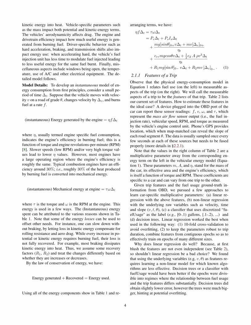
Figure 4: Comparing actual stops (speed < 5 mph) with those inferred fromthe map.

able, the remapping can predict fuel usage apriori and onroads that were not observed before by Sparc.Inadequacies: Maps only have static information such asspeed limit, slope and stop light information. But, fuel usedepends on the changes in speed: kinetic energy depends di-rectly on the change in speed and terms like aerodynamicdrag ∝ v3 vary substantially with small changes in veloc-ity. 3 Hence, using the speed limit as GreenGPS [16] doesleads to sizable error.

Measurements from our deployment help quantify thisproblem. Figure 3 (left) compares average speed on a roadsegment with the posted speed limit on that segment. Theplot on the right depicts the standard deviation in speeds ob-served on that road segment vs. the average observed speed.Note that the actual speed on a segment is correlated to theposted limit but there is substantial noise.

Stop lights are another complication. Figure 4 comparesthe actual stops observed in a trip with the inference fromthe map. We say that a vehicle is stopped if the speed fromGPS is below 5 mph. The actual stops can be less than thatestimated from the map (e.g., traffic signal is green) or manymore (e.g., due to congestion). In our dataset, we see bothtypes. Worse, not every stop costs the same amount of en-ergy. Stops on higher speed roads have a larger effect sincemore kinetic energy is lost per stop.

Remapping: We realize from above that there is at best atenuous connection between map info per road segment andthe desired features (Table 2 that correlate with fuel usage).However, our key insight is that similar road segments havesimilar desired features. That is the desired features of asegment with posted speed limit of 40mph, 2% grade, with ahighway on one end and a stop light at the other are likely tobe similar to another segment with the same characteristics!With just a few drivers, Sparc already has ground-truth fea-tures for tens of thousands of road segments. This set is largeenough that any unseen road segment has a large number ofsimilar segments for which features are available.

Hence, Sparc’s strategy to remap is (a) given a route onthe map, obtain from the map the information shown in Ta-ble 3 for each road segment along the route, (b) add time-of-day/ day-of-week values to capture congestion, and (c)

3say vehicle has speed 1 and 2 for unit time each; aerodrag ∝∑v3t = 9; but, using average velocity leads to 2 ∗ (1.5)3 = 6.75

6

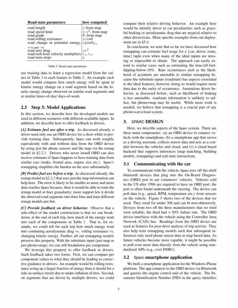
Road-state parameters how computedroad length x from maproad speed limit v, v2, from maproad grade θ, from maproad rolling resistance x cosθroad change in potential energy,+’ve and -’ve

x[sinθ]0+

road aero drag xv2

road rush hour velocity multipliers rv, rv2

road num stops s

Table 3: Road state parameters

use training data to learn a regression model from the val-ues in Table 3 to each feature in Table 2. An example suchmodel would compute how much energy will be spent inkinetic energy change on a road segment based on the ki-netic energy change observed on similar road segments andat similar times-of-day/ days-of-week.

2.3 Step 3: Model ApplicationsIn this section, we describe how the developed models areused in different scenarios with different available inputs. Inaddition, we describe how to offer feedback to drivers.

[A] Estimate fuel use after a trip. As discussed already, adriver need only use an OBD device for a short while to pro-vide training data. Subsequently, Sparc can work roughlyequivalently with and without data from the OBD deviceby using just the phone sensors and the map via the remapmodel in §2.2.1. Drivers who never install OBD can alsoreceive estimates if Sparc happens to have training data fromsimilar cars (make, frontal area, engine size etc.). Sparc’sremapping simplifies the burden on the user substantially.

[B] Predict fuel use before a trip. As discussed already, theremap model in §2.2.2 that uses just the map information canhelp here. The error is likely to be smaller as more and moredata reaches Sparc because, then it would be able to train theremap model at finer granularity; more support lets it dividethe observed road segments into finer bins and train differentremap models per bin.

[C] Provide feedback on driver behavior. Observe that aside-effect of the model construction is that we can break-down, at the end of each trip, how much of the energy wentinto each of the components in Table 1. That is, for ex-ample, we could tell for each trip how much energy wentinto combating aerodynamic drag vs. rolling resistance vs.changing kinetic energy. Further, all our remapping modelspreserve this property. With the substitute input (just map orjust phone+map), we can still breakdown per component.

We leverage this property to offer feedback to drivers.Such feedback takes two forms. First, we can compare percomponent values to what they should be leading to correc-tive guidance to drivers. An example would be rolling resis-tance using up a larger fraction of energy than it should for aride on surface streets due to under-inflation of tires. Second,on segments that are driven by multiple drivers, we could

compare their relative driving behavior. An example herewould be identify driver or car peculiarities such as grace-ful braking or aerodynamic drag that are atypical relative toother drivers/cars. More specific examples from our deploy-ment are in §5.4.

In conclusion, we note that so far we have discussed howremapping can estimate fuel usage for a {car, driver, route,time} tuple even when many of the ideal inputs are miss-ing or impossible to obtain. The approach can easily ex-tend to similar cases such as estimating the time-till-fuel-dipping-below-10%. Rare occurrences such as the likeli-hood of accidents are amenable to similar remapping be-cause the substitute inputs (roadstate) has aspects correlatedto the ideal features; however, doing so would require moredata due to the rarity of occurrence. Anomalous driver be-havior, as discussed before, such as likelihood of brakingis less amenable: roadstate information is unlikely to suf-fice, but phone+map may be useful. While more work isneeded, we believe that remapping is a crucial part of anyphone+car+cloud system.

3. SPARC DESIGNHere, we describe aspects of the Sparc system. There are

three main components: (a) an OBD device to connect ve-hicle with the smartphone, (b) a smartphone app that servesas a driving assistant, collects sensor data and acts as a con-duit between the vehicles and cloud, and (c) a cloud basedbackend that supports inferences (map matching, buildingmodels, remapping) and real-time interactions.

3.1 Communicating with the carTo communicate with the vehicle, Sparc uses off-the-shelf

bluetooth devices that plug into the On-Board Diagnos-tics (OBD) port in our volunteers’ vehicles. Vehicles soldin the US after 1996 are required to have an OBD port; theport is often found underneath the steering. The device canpoll data (e.g., speed, RPM, temperature etc.) from sensorson the vehicle. Figure 5 shows two of the devices that weused. They retail for under 30$ and can fit non-obtrusively.Devices from two off the three manufacturers that we triedwere reliable; the third had > 50% failure rate. The OBDdevice interfaces with the vehicle using the Controller AreaNetwork (CAN) bus. Readings from the OBD device areused as features for post-drive analysis of trip activity. Theyalso help train remapping models such that subsequent in-ferences only need phone sensor data or map based data. Asfuture vehicles become more capable, it might be possibleto poll even more data directly from the vehicle using stan-dardized APIs (e.g., over DSRC).

3.2 Sparc smartphone applicationWe built a smartphone application for the Windows Phone

platform. The app connects to the OBD device via Bluetoothand queries the engine control unit of the vehicle. The Pa-rameter Identification Number (PID) in the query identifies

7

Figure 5: OBD-II devices used

the information requested (e.g., 010D for speed). Vehiclemanufacturers implement several proprietary PIDs but to bebroadly applicable we only rely on the PIDs in the OBD-IIstandard. Some vehicles do not have the sensors needed forsome PIDs; for e.g., some Audi models do not have the fuelinjection sensor. Further, sensor values update at differenttimescales and queries on some (older) cars take over 10xlonger than normal for the same PID. Hence, our app firstsweeps the PID space to identify PIDs that offer non-trivialresponses and the frequency at which they update. Then,it generates a polling schedule such that the more relevantPIDs (e.g., speed, torque, fuel) are polled at least once everyfew seconds. To compare, polling all the standard PIDs in around-robin manner retrieves much less information 4.

To appeal to driving aficionados, a live dashboard in theapp displays some of the information from OBD-II (see appscreen-shots in Fig. 6).

Bluetooth usage is not a problem. Surprisingly, we foundthat even when our app is connected to the OBD device, thephone can establish other Bluetooth connections to say head-sets or the car speakers. Thus, the app does not disrupt theseactivities. This is because Bluetooth allows one connectionper profile at a time; and OBD devices have a profile differ-ent from these other devices.

To be widely useful, the app has to satisfy a few con-straints. First, it should be able to run continuously in thebackground and collect data whenever in a moving vehicle.Otherwise, the app will either miss rides or drain the battery.In an earlier version we found that users remembered to turnthe app on (or off) less than 20% of the time. Second, theapp’s power drain should be an insignificant fraction of thetotal power draw. Typical users drive a car for less than twohours a day; so two hours of data collection (and 22 inac-tive hours) should cost say less than 10% of the day’s powerdraw. Third, to preserve volunteer’s privacy, the app shouldallow scrub personally identifiable information such as loca-tion of homes and destinations.

Energy management. Our app, as implemented, achievesmost of the aforementioned goals. The application staysinactive in the background consuming almost zero energywhile the phone is stationary. A minimal background taskperiodically searches for a Bluetooth paired OBD device andwakes up the app when it succeeds. This lets us catch ev-ery trip; it is implementable on different platforms unlikethe significant location change trigger (only iOS) and is lesspower hungry than continuously processing the accelerom-

4in the information theoretic sense

Figure 6: Screen-shots of our app.

eter to detect movement. On windows phone 8.0, the appis ejected after four hours of inactivity; hence, we toast theuser to restart the app. The app goes back to sleep when itsenses that the vehicle is no longer moving (based on a dis-tance traveled and speed check). Across all of the deployedusers, the average power draw is 0.4%/ minute when app isawake and 0.01%/ hour otherwise. The app is awake on av-erage for 35 minutes each day. Logs are uploaded to Azurelazily when the device is connected over WiFi and sufficientbattery charge remains.

3.3 Cloud servicesThe Azure based services manage the data collection ac-

tivities from the users’ smartphones. It is also responsiblefor map-matching and providing the features for the map-only remapping model (§2.2.2). We use OpenStreetMapsand maps from a proprietary vendor to build these models.We map-match, i.e., from GPS location readings, we iden-tify the most likely path along road segments through an in-ference algorithm that is similar to Viterbi decoding. Othercloud services include a public-portal for our users wherethey can view and analyze their driving history.Building models. The server also coalesces data from mul-tiple users and vehicles to train and build models for Sparcbased applications. These models (e.g., for inference remap-ping) become more accurate as the server gathers higher vol-ume of data from the drivers’ phones and vehicles. In sec-tion §5.4.2, we discuss how much training data is necessary.Remapping also enables Sparc to offer value to drivers andvehicles that use the system with just the smartphone appli-cation. Till date, we have collected more than 4,400 miles ofdata from 20 vehicles. The deployment and user study wereconducted under purview of Microsoft Research’s privacypolicy. We plan to release the Sparc smartphone applicationin the app store before publication date.

3.4 Beyond fuel predictionOur phone+car+cloud architecture lets us build a set of

diverse applications. We have already implemented a hand-ful in addition to trip analytics, fuel usage prediction anddriving feedback. They include a a location based real-timetraffic alerter (using the Bing Maps API). Also, a "FindMy-Car" button that shows a user where her car is parked. We

8

Figure 7: Breakdown of miles traveled in dataset along various aspects.

say that a car is present near the last (first) GPS reading ob-tained by our smartphone app before (after) it lost access tothe OBD device, which happens when the engine turns on-> off. We note some limitations for this heuristic; in partic-ular it cannot disambiguate between floors in multi-tiered orunderground parking lots. Finally, a website that (1) offersFindMyCar from a browser, (2) visualizes the user’s trips ona map and (3) offers some longitudinal analysis about driv-ing patterns and energy use.

4. DEPLOYMENT & MEASUREMENTSIn this section, we present details about our system deploy-ment. We point out the diversity across cars (makes, years)and roads (re: speed, grade and congestion).

4.1 System DeploymentWe deployed our app and OBD devices to twenty volunteersand collected data from Aug. 2013 to Dec. 2014. The vol-unteers drove a total of 151 hours covering 4423 miles and15846 unique road segments. The system deployment is un-der the approval of an internal review board supervised byour organization’s privacy team.

Figure 7 shows a break down of the the miles traveled bythe volunteers in our dataset based on various aspects. Wesee a wide range of manufacturers and engine sizes varyingfrom small sedans (≤ 2 liter engines) to large SUVs (> 3liter engines). Roughly half of the miles were from roadswith non-trivial banking grade (θ > 1o). Also, roughly halfare at speeds below and above 40 miles-per-hour (mph), in-dicating a mix of highway and surface-road miles.The topfifteen drivers contributed most of the data. Figure 8 vi-sually depicts all the road segments that we have collecteddata over; the color of a road segment indicates the numberof distinct drives through that segment.

4.2 Challenges and opportunities in estimat-ing fuel usage

Predicting fuel usage would be simplest if a vehicle alwaysoperated at the same fuel efficiency. Figure 9 shows the per-vehicle distribution of fuel efficiency (MPG). We see thatfor a majority of cars, their inter-quartile difference is largerthan 30% of their average. In fact, for over 70% of the cars,the observed median fuel efficiency was outside the range in-dicated by EPA’s MPG estimates for city and highway use.The median was away by up to 10 MPG. Note that the range

Figure 8: Routes traversed by our drivers in two cities; darkness of the colorindicates the number of distinct trips per segment.

0

10

20

30

40

50

0 2 4 6 8 10 12 14 16

MPG

Car Id

Figure 9: Distribution of fuel efficiency (Miles per Gallon) across vehiclesin dataset. The 10th, 25th, 50th, 75th and 90th percentile values are shown.

is quite large to begin with since the MPG estimate for citydriving is often 6− 10 MPG less than the highway estimate.To understand further, Figure 10 plots the fuel used vs. dis-tance traveled in contiguous two minute periods. The pointsappear to cluster into two groups; those on the right are fromfaster roads. However, even within each group, there is sub-stantial variation. This means that predictions based on ex-pected MPG are unlikely to be useful.

We next consider trips between the same begin and endlocations. When driving within a metropolitan area, thereare often a handful of usable routes to take between a givenpair of locations. The route that a driver picks impacts fueluse. For the same route, varying congestion levels wouldimpact fuel use. Finally, the variation is likely to be largerwhen multiple cars are considered, owing to different cartypes and driving styles. Figure 11 plots the ratio of thefuel used in a trip by the average fuel used by all trips be-tween the same locations. Figure 12 computes the numberof rides that are off by more than a given error thresholdfrom the average. We see that even when limited to trips

0

0.02

0.04

0.06

0.08

0.1

0.12

0.14

0 0.5 1 1.5 2 2.5 3

Fuel u

sed (

gallo

ns)

Distance traversed (miles)

Figure 10: Fuel use vs. distance travelled in a 2 min. period across all cars

9

0 0.1 0.2 0.3 0.4 0.5 0.6 0.7 0.8 0.9

1

0 0.5 1 1.5 2 2.5 3

Cum

ula

tive

(

fract

ion o

f all

rides)

Fuel use of ride divided by Avg. fuel use of all rides b/w the same locations

Indiv. CarsAll Cars

Figure 11: Even trips between the same begin and end points have substan-tial differences in fuel used

Figure 12: For trips between the same begin and end points, the fractionthat are outside a given error threshold from the average

for the same car (and driver), 31% (9%) of trips are off bymore than 20% (50%) of the average. The average error onlybecomes larger when trips from all cars are included. Thisillustrates both the challenge and the promise: even for thesame car and route, fuel use varies substantially; however, ifonly accurate predictions were available, choosing the bestfrom among the different routes between a pair of locationscan reduce fuel use substantially.

5. EVALUATIONIn this section, we evaluate the accuracy of our physicalmodel for fuel usage. We show that our physical model thatuses data from the OBD port of cars helps us estimate fuelusage with less than 3% average error. Through inferenceremapping we show that we can use data from phone sen-sors to estimate fuel usage with less than 6% average error(compared to the ground truth). By remapping to the road-state data, we also show that we can predict fuel use beforea trip with ≤20% error on the 85th percentile trip. We alsodescribe some interesting feedback on driver behavior.

Qualitative comparison. Before delving into the numbers,we first qualitatively compare Sparc with related researchand commerical systems. Table 5 presents this compari-son. GreenGPS [16] estimates fuel usage given OBD train-ing data. However, it does not provide feeedback re: driv-ing behavior and since it does not remap the roadstate in-puts, its error is very high when OBD data is not available.CMT [10] focuses on risk profiling drivers based on smart-phone sensors only; it examines aspects such as hard accel-eration/ driving above speed limit and offers insights to bothdrivers and insurance companies. However, CMT does notconsider fuel consumption and does not connect with the car.Automatic [6] and Mojio [24] use OBD, an app and cloud

connectivity to provide trip analytics, vehicle diagnostics in-formation and location-related applications. While Sparc of-fers similar services, our inference remapping deals betterwith missing data sources (e.g., no OBD device) and henceis likely to be more widely usable.

5.1 MethodologyDataset: We use the traces collected from unconstraineddrivers that we described in §4.1 for this analysis.Metrics: Per trip, we measure the error in estimating fuelused:

relativeerror = 100 ∗ estimate− actualactual

.

The estimate can either be generated before the trip wastaken, i.e., a prediction, or could be computed post-factofrom the sensor readings obtained during the trip. When thesign of the error is not relevant, we show the absolute valueof the relative error. Per driver and given a collection of trips,we also compute the contribution to fuel usage due to eachof the major components: rolling resistance, increasing po-tential energy, increasing kinetic energy, aerodynamic loss,idling and the others. We also estimate the net positive con-tribution from the decreases in potential and kinetic energy(e.g., rolling downhill requires less fuel to maintain speed).Compared alternatives: We have a choice in how the tripfeatures are obtained, how the car-specific parameters areobtained, and how both are combined. In our experimentalresults, OBD features and Phone features refer to trip featurescomputed based on sensor readings from the correspondingdevice (see Table 2). Road features refers to trip features com-puted based on data from the map (see Table 3). Further,OBD parameters and Phone parameters refer to the car param-eters that are used in the physical model derived from OBDfeatures (§2.1) and the remapped model based on the Phonefeatures (§2.2.1), respectively. By Stock parameters, we referto car parameters that are obtained from automobile specifi-cations. Finally, Road→Phone features refer to parameters ofthe remap model that relies on just map information (§2.2.2).

Not all of the parameter+feature combinations are inter-esting. We use the combinations that are most relevantper §2.3 for our evaluation.

• SR refers to using the stock car parameter along withthe road features in the physical model. Withoutremapping, this is the best one could do for predictionand post-facto estimates.

• OO refers to using the OBD parameters along with theOBD features in the physical model. We expect thiscombination to have the smallest error. Fuel usage isdirectly estimatable given OBD data. So, the value ofthis datapoint is primarily to check the correctness andcompleteness of the physical model.

• PP refers to applying the phone parameters along withthe phone features in the physical model. Both OO andPP are only usable post-facto, i.e., after the drive, sincethe features are not available apriori.

10

Section Experiment Summary of ResultsApplication 1: Post-drive fuel usage prediction§5.2 (Fig 13) Estimating fuel consumption after a drive us-

ing smartphone + OBD model vs. smart-phone only model.

For estimation intervals over 100 sec., (a) average error < 7% using smart-phone only. Using both OBD + smartphone, average estimation error < 2%for 100 sec. intervals and < 6% for 10 sec. intervals.

Application 2: Pre-drive fuel usage prediction§5.3 (Fig 14) Estimating fuel consumption before a drive. Using road state model to covert road features into phone features (PhRPh)

results in < 20% errors for 48% trips. Better than the baseline (PIR) and otherschemes (PhR, OR) which have < 20% errors for 13%, 11% and 12% tripsrespectively.

Application 3: Analyzing driving behavior§5.4 (Fig 16) Analyzing driving behavior impact on fuel

consumption for the same trip.Our model identifies driver’s impact on different fuel consumption factors(e.g., resuable kinetic loss, using older tires). We identified drivers whosegentle braking behavior enabled resuse of vehicle’s kinetic energy.

§5.4.1 (Fig 17) Per-user long term driving impact on fuelconsumption.

Analyzing kinetic energy re-use resulted in idenfying drivers with gentlebraking and its impact on fuel consumption. Insights about the impact ofdrivers’ most frequent commutes on overall fuel consumption.

Table 4: Summary of evaluation results.

Features Us CMT [10] GreenGPS [16] Mojio [24]Analyze driving X XbehaviorCan drive X X Xwithout OBDAnalyze fuel X X Xconsumption

Table 5: Comparing features of Sparc vs. other applications.

0

5

10

15

20

25

30

35

10 20 30 40 60 80 100

Est

imat

ion E

rror

(%

)

Latency (Seconds)

OBD ModelPhone Model

Figure 13: Estimating fuel consumed during a trip using data from (a) theOBD device and phone (2) the phone alone. We can estimate the fuel con-sumed during a trip with good accuracy using only the phone. The variationshown is across different drivers.

• PRP refers to using the phone parameters and theroad→Phone features. This is usable for predictionsince it only uses road features at runtime. 5

Table 4 summarizes our evaluation results.

5.2 Estimating Fuel Use After a TripAfter completing a trip, can we measure the amount of fuelconsumed during the trip? This is of some value to a driver;she can estimate how much emissions her driving caused.It may be especially useful when the tank is nearly empty.Even this simple use-case is not possible today without in-stalling an OBD device. Using inference remapping, we canestimate fuel use using data from phone sensors.

Figure 13 plots the absolute value of estimation error vs.the duration that the estimate was computed over for boththe OBD model (OO) and the Phone model (PP). Per car,we compute the average error over all non-overlapping con-tiguous traces of a given duration. The error bars show the5 We skip Road→OBD features and ORO which applies the OBDparameters on the road features since the results are similar to PRP.

quartiles and min, max across drivers. Most trips last wellover 100s; here, PP yields an average error of 7%. Allthe cars have less than 10% error. Comparatively OO hasa much smaller error, 2% at 100s and just 6% for 10s in-tervals. Recall that if an OBD device is installed, the fuelusage is directly available. Rather, we compute the error ofOO to sanity check our models. We conclude that for mosttrips just the data available from the smartphone suffices toobtain highly accurate estimates.

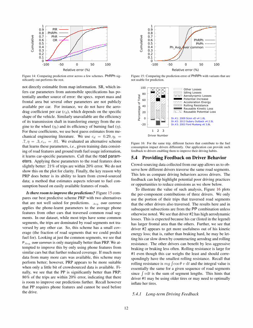
5.3 Predicting Fuel Use Before a TripIn this section, we evaluate our ability to predict fuel us-age. In our dataset, we observe that a large fraction of thetrips that drivers take involve road segments that were nottraversed before. Hence, we are more interested in predict-ing fuel for such cases. Figure 14 depicts the error for afew schemes. Recall that PRP first uses the road-state modelto remap road features (from a map) to phone features; towhich it then applies the car parameters learnt using trainingdata from the phone. We see that for 49% of the trips, theirpredictions of fuel usage are within 20% error (gray regionin figure). This is significantly better than the results for thebaseline (SR) and the other predictive schemes (PR, OR).The fraction of trips that can be predicted to within 20% er-ror are 13%, 11% and 12% respectively for these schemes.We see that about 4× more trips can be predicted to within20% error by PRP.

It is interesting to note that related pieces of work for fuel-use estimation like GreenGPS [16] learn the vehicular modelfrom OBD data but cannot extract features for unseen roads.Hence, its performance is slightly worse than that shown forOR. Worse because their energy model relies on average ve-locity rather than piece-wise integrals (§2.2.1). Further theydo not separate out the positive and negative parts of changesto potential and kinetic energy which is important as we seenext when consider per-component contributions.

Why does using the road features, readily available fromthe map, lead to such poor predictions? This is because,as we saw in §2, the actual speed for a driver on a roadsegment can be very different from the posted speed limit;and variations in speed due to acceleration and braking are

11

0 0.1 0.2 0.3 0.4 0.5 0.6 0.7 0.8 0.9

1

-100 -50 0 50 100

Cum

ula

tive

Relative error (%)

PlRPhRPh

PhROR

Figure 14: Comparing prediction error across a few schemes. PhRPh sig-nificantly out-performs the rest.

not directly estimable from map information. SR, which in-fers car parameters from automobile specifications has po-tentially another source of error: the specs. report mass andfrontal area but several other parameters are not publiclyavailable per car. For instance, we do not have the aero-drag coefficient per car (cd), which depends on the specificshape of the vehicle. Similarly unavailable are the efficiencyof its transmission shaft in transferring energy from the en-gine to the wheel (ηt) and its efficiency of burning fuel (η).For these coefficients, we use best guess estimates from me-chanical engineering literature. We use cd = 0.29, ηt =.7, η = .3, crr = .01. We evaluated an alternative schemethat learns these parameters, i.e., given training data consist-ing of road features and ground truth fuel usage information,it learns car-specific parameters. Call that the road param-eters. Applying these parameters to the road features doesslightly better: 21% of trips are within 20% error. We do notshow this on the plot for clarity. Finally, the key reason whyPRP does better is its ability to learn from crowd-sourceddata; a method that estimates aspects relevant to fuel con-sumption based on easily available features of roads.

Is there room to improve the predictions? Figure 15 com-pares our best predictive scheme PRP with two alternativesthat are not well suited for predictions. Avg. over commonapplies the phone-learnt parameters to the average phonefeatures from other cars that traversed common road seg-ments. In our dataset, while most trips have some commonsegments, the trips are dominated by road segments not tra-versed by any other car. So, this scheme has a small cov-erage (the fraction of road segments that we could predictfuel for). Looking at just the common segments, we see thatPAvg. over common is only marginally better than PRP. We at-tempted to improve this by only using phone features fromsimilar cars but that further reduced coverage. If much moredata from many more cars was available, this scheme mayperform better; however, PRP appears to be more suitablewhen only a little bit of crowdsourced data is available. Fi-nally, we see that the PP is significantly better than PRP:86% of the trips are within 20% error, indicating that thereis room to improve our predictions further. Recall howeverthat PP requires phone features and cannot be used beforethe drive.

0 0.1 0.2 0.3 0.4 0.5 0.6 0.7 0.8 0.9

1

-100 -50 0 50 100

Cum

ula

tive

Relative error (%)

PhRPhPhPh

Ph_Avg. over common

Figure 15: Comparing the prediction error of PhRPh with variants that arenot usable for prediction.

-20

0

20

40

60

80

100

1 2 3

Perc

enta

ge o

f Tota

lDriver Number

Dr.#1: 2009 Scion xD v4 1.8LDr.#2: 2013 Subaru Outback v4 2.5LDr.#3: 2003 Ford Mustang v6 3.8L

Reusable Potential LossReusable Kinetic LossRolling ResistanceAcceleration EnergyPotential IncreaseAerodynamic LossesIdling LossesOther Losses

Figure 16: For the same trip, different factors that contribute to the fuelconsumption impact drivers differently. Our application can provide suchfeedback to drivers enabling them to improve their driving habits.

5.4 Providing Feedback on Driver BehaviorCrowd-sourcing data collected from our app allows us to ob-serve how different drivers traverse the same road segments.This lets us compare driving behaviors across drivers. Thefeedback can help highlight potential poor driving practicesor oppurtunities to reduce emissions as we show below.

To illustrate the value of such analysis, Figure 16 plotsthe per-component contributions of three drivers. We onlyuse the portion of their trips that traversed road segmentsthat the other drivers also traversed. The results here and insubsequent subsections are from the PP combination unlessotherwise noted. We see that driver #2 has high aerodynamiclosses. This is expected because his car (listed in the legend)has larger frontal area than the others. Further, we see thatdriver #2 appears to get more usefulness out of his kineticenergy loss; that is, rather than braking hard, he may be let-ting his car slow down by counteracting aerodrag and rollingresistance. The other drivers can benefit by less aggressivebraking or braking less often. Rolling resistance is large for#1 even though this car weighs the least and should corre-spondingly have the smallest rolling resistance. Recall thatrolling resistance is mg

∫cos θ v dt and the integral value is

essentially the same for a given sequence of road segmentssince

∫vdt is the sum of segment lengths. This hints that

driver #1 may be using older tires or may need to optimallyinflate her tires.

5.4.1 Long-term Driving Feedback

12

-20

0

20

40

60

80

100

1 2 3 4 5 6 7 8

Perc

enta

ge o

f To

tal

Driver Number

Dr.#1: 2009 Scion xD v4 1.8LDr.#2: 2013 Subaru Outback v4 2.5LDr.#3: 2003 Ford Mustang v6 3.8LDr.#4: 2011 Acura TSX v4 2.4LDr.#5: 2013 Chevrolet Cruze v4 1.4LDr.#6: 2011 Toyota Highlander v6 3.5LDr.#7: 2011 Lexus RX 350 v6 3.5LDr.#8: 1999 Lexus GS 400 v8 4.0L

Reusable Potential LossReusable Kinetic LossRolling ResistanceAcceleration EnergyPotential IncreaseAerodynamic LossesIdling LossesOther Losses

Figure 17: Drivers can also use our application to build up customized long-term driving profiles that average out trip-level dynamics such as traffic,road, and weather conditions.

Analyzing all the data from a given car can reveal furtherinsights specific to driving behavior. Figure 17 plots theper-component contributions for the eight drivers who con-tributed the most data; we ignore the others for clarity. Con-sider driver #6, who has a large hybrid SUV. Her daily com-mute involves climbing a steep hill near her residence; con-sequently she spends the most fuel in going uphill (potentialincrease). We see that she is able to make more use of theloss in kinetic energy (KE) because her car explicitly recap-tures what would otherwise be lost as heat upon braking tocharge the battery instead. Driver #8 does not have a hybridbut appears to be by far the gentlest user of brakes; insteadreducing his KE by making it work against the other losses.Consider driver #7, who also has a large SUV but primarilyuses it to commute from a suburb to the city on a major high-way. We see that rolling resistance and aerodynamic lossesdominate; this is expected because most of his driving oc-curs at higher speeds, involves long distances and his carhas a large frontal area. Comparatively, he spends less fuelin increasing KE (acceleration energy), hinting that most ofhis drives are at relatively steady velocity. Not much changein PE either, because his trips, in the midwest, are on flatroads. Consider driver #4, who has a smaller wagon andalso mostly commutes on a congested highway. His com-ponent breakdown is similar to that of driver #7 except fora larger contribution due to increasing KE. Perhaps conges-tion causes him to change speed often. In contrast driver #1uses a sub-compact for a long commute and some errandson surface streets. We see that rolling resistance is dominantfor her; aerodrag is small due to the slower speeds and smallfrontal area.

5.4.2 How Much Training Data Do We Need?To answer this question, we vary the sizes of training data.Per size, we pick a random subset to be the training data,learn the car-specific parameters from this set and applythese parameters to the rest of the data to estimate per-component contributions. We repeat this for 100 randomsubsets. When training is done on enough data, we wouldexpect that the parameters learnt from the different training

-20

0

20

40

60

80

Rolling Resist.

Reuse.Kin.Loss

Acceleration

Potential Inc.

Reuse.Pot.Loss

Aero.Drag

Idling Losses

Other Losses

Perc

enta

ge

of T

otal

Variation in Energy Components vs. Amount of Modeling Data (For Dr.#2: 2013 Subaru Outback v4 2.5L)

0.2 Hrs.0.5 Hrs.1.0 Hrs.2.0 Hrs.4.0 Hrs.6.0 Hrs.8.0 Hrs.

Figure 18: For driver 2, to build a reliable long-term profile, we need tocollect about four hours of data and build the regression model.

subsets to be similar, i.e., they report similar per-componentcontributions. However, when trained on too little data, theper-component contributions could be very different.

Figure 18 plots the quartiles, min and max of theper-component contributions for driver #2 given differentamounts of training data. We report results for this driverbecause he had the most data; however other drivers yieldedsimilar results. We see that some components can be esti-mated correcly with fewer data than others. When too littledata is used, most components exhibit variability. Because,the model may be influenced by the specific roads and traf-fic conditions present in the training data. Such models arelikely to have little predictive value. However when morethan four hours of data is used for training we find that mostcomponents are stable. These training sets are perhaps largeenough to be representative of typical driving conditions.This leads us to conclude that about four hours of trainingdata should suffice for most drivers.

6. RELATED WORKA driver cares about two aspects of vehicular fuel use: (1)how much fuel would a trip use and (2) what factors impactfuel efficiency?

The conventional metric for fuel efficiency in the UnitedStates (US) is miles per gallon (MPG). While MPG is ade-quate to compare vehicles, we saw that it neither helps pre-dict fuel use on a trip nor explains the factors impacting fuelefficiency [21]. The environmental protection agency (EPA)is tasked with determining MPG estimates and publishes anannual document outlining its methodology [5]. In responseto widespread criticism– estimates lacked real-world test-ing, and were of very limited scale i.e., city or highway –EPA updated its rating system in 2008. The new systemconsiders things like faster speeds, acceleration, air condi-tioner use, and colder outer temperatures [13]. While animprovement, they still do not suffice for the above goals.In particular, MPG estimates are inadequate at capturing thevariable traffic and road conditions [2, 14, 4]. To remedythis, much focus has gone into gathering and collecting real-world user data re: fuel efficiency [12, 27]. Unfortunately,the user-reported numbers exhibit substantial variability [12]

13

and lack the context that may help explain the variability.Concluding that static MPG estimates are unreliable, fo-

cus has shifted towards dynamic models of fuel efficiency.One class of work empirically determines an MPG esti-mate per driving regime such as constant speed, high ac-celeration, peak-traffic times, highway or city etc. [9, 7,17]. While more accurate, these estimates do not explainfactors that impact fuel economy nor can they predict fuelconsumption accurately. Another class of work developsdynamic fuel-estimation models using several parameters.Some of these approaches require elaborate instrumenta-tion to measure parameters such as exhaust-gas composi-tion and engine-cylinder displacement [1]. The more prac-tical approaches use OBD information available in modernautomobiles [3, 16, 15]. These methods collect OBD-datafrom individual drivers and build fuel-estimation models.GreenGPS [16] is the best example here.

However, these approaches still have a few drawbacks.First, they can analyze fuel use post-facto but cannot predictfuel use before a trip, especially if the road segments havenot been driven on before. Second, lacking the ability to ex-trapolate, they require drivers to continually use an OBD de-vice. Third, when using the models to extract per-componentcontributions, we find that errors in the models (e.g., usingaverage values, not separating loss of energy terms) leadsto mis-attributions. The approach presented here addressesthese shortcomings. It allows users with a smartphone de-vice to obtain accurate estimates of MPG values and offersinsight into the factors affecting fuel economy. And, it canpredict fuel use before a trip occurs; fuel-prediction also dis-tinguishes us from other mobile participatory sensing sys-tems that use smartphone devices to generate traffic advi-sories [20, 19] or manage parking [11].

7. CONCLUSIONWe describe a phone+car+cloud system that has the po-

tential to transform many vehicular use cases. Our coretechnical contribution is the concept of inference remappingwhich allows us to compute inferences even when the idealinputs are missing or impossible to obtain apriori. For e.g.,given readings from a smartphone, we can estimate fuel usedby a vehicle. Further, given some crowd-sourced data, wecan predict fuel used along a route for whom no data read-ings have been collected. At first blush, both seem impos-sible. Yet, remapping makes this possible. Because, weare able to exploit underlying correlations between readilyavailable information (e.g., maps), training data, and the de-sired information that captures vehicular fuel use (e.g., dy-namic changes in speed, stop durations, car parameters etc.)Careful engineering was required to compose disparate time-series and to not overwhelm phone battery. Much work re-mains, in particular, Sparc’s predictions remain 1.8X awayfrom the post facto estimates. Also, whether remapping isbroadly applicable remains an open question.

8. REFERENCES

[1] K. Ahn. Microscopic fuel consumption and emissionmodeling. PhD thesis, Virginia Polytech. Inst. andState Univ., 1998.

[2] W. M. Al-Momani and O. O. Badran. Experimentalinvestigation of factors affecting vehicle fuelconsumption. Int. J. Mech. and Materials Eng., 2007.

[3] F. An and M. Ross. Model of fuel economy withapplications to driving cycles and traffic management.Transportation Research Record, 1993.

[4] S. T. Anderson et al. Automobile fuel economystandards: Impacts, efficiency, and alternatives. Rev.Environmental Economics and Policy, 2010.

[5] A. Atabani et al. A review on global fuel economystandards, labels and technologies in the transportationsector. Renewable and Sustainable Energy Rev., 2011.

[6] Automatic. Available Online at:https://www.automatic.com/.

[7] J. Bandeira et al. A comparative empirical analysis ofeco-friendly routes during peak and off-peak hours. InAnn. Meet. Transportation Research Board, 2012.

[8] C. Baumgarten. Mixture formation in internalcombustion engines. 2006.

[9] M. Ben-Chaim, E. Shmerling, and A. Kuperman.Analytic modeling of vehicle fuel consumption.Energies, 2013.

[10] Cambridge Mobile Telematics. Available Online at:http://www.cmtelematics.com.

[11] V. Coric and M. Gruteser. Crowdsensing maps ofon-street parking spaces. In DCSS, 2013.

[12] EPA shared MPG estimates. Available Online at:http://www.fueleconomy.gov/mpg/MPG.do?action=browseList.

[13] EPA fuel economy guide. Available Online at:http://www.fueleconomy.gov/feg/printGuides.shtml.

[14] E. Ericsson. Variability in urban driving patterns.Transportation Research Part D: Transport andEnvironment, 2000.

[15] Fuelly. Available Online at: https://www.fuelly.com/.[16] R. K. Ganti et al. GreenGPS: A participatory sensing

fuel-efficient maps application. In MobiSys, 2010.[17] Gas buddy. Available Online at:

http://www.gasbuddy.com/.[18] J. S. Greenfeld. Matching gps observations to

locations on a digital map. In Ann. Meet.Transportation Research Board, 2002.

[19] S. Hu et al. Poster abstract: Smartroad: Acrowd-sourced traffic regulator detection andidentification system. In IPSN, 2013.

[20] E. Koukoumidis et al. SignalGuru: Leveraging mobilephones for collaborative traffic signal scheduleadvisory. In MobiSys, 2011.

[21] R. P. Larrick and J. B. Soll. The MPG illusion. Science20, 2008.

[22] A. Mai and D. Schlesinger. A business case for

14

connecting vehicles executive summary. CISCOInternet Business Solutions Group Report, Apr. 2011.

[23] Metromile. Available Online at:https://www.metromile.com/.

[24] Mojio. Available Online at: https://www.moj.io/.[25] S. Nath. ACE: exploiting correlation for

energy-efficient and continuous context sensing. InMobiSys, 2012.

[26] J. Paek, J. Kim, and R. Govindan. Energy-efficientrate-adaptive gps-based positioning for smartphones.In Mobisys, 2010.

[27] M. Satyanarayanan. Mobile computing: The nextdecade. ACM Mobile Comp. and Comms. Rev., 2011.

15