Embed Size (px)
Citation preview
Inference Over the Web
Stefan Schoenmackers
A dissertation submitted in partial fulfillmentof the requirements for the degree of
Doctor of Philosophy
University of Washington
2011
Program Authorized to Offer Degree: Computer Science and Engineering


University of WashingtonGraduate School
This is to certify that I have examined this copy of a doctoral dissertation by
Stefan Schoenmackers
and have found that it is complete and satisfactory in all respects,and that any and all revisions required by the final
examining committee have been made.
Co-Chairs of the Supervisory Committee:
Oren Etzioni
Daniel S. Weld
Reading Committee:
Oren Etzioni
Daniel S. Weld
Jesse Davis
Date:


In presenting this dissertation in partial fulfillment of the requirements for the doctoraldegree at the University of Washington, I agree that the Library shall make its copiesfreely available for inspection. I further agree that extensive copying of this dissertationis allowable only for scholarly purposes, consistent with “fair use” as prescribed in the U.S.Copyright Law. Requests for copying or reproduction of this dissertation may be referredto Proquest Information and Learning, 300 North Zeeb Road, Ann Arbor, MI 48106-1346,1-800-521-0600, to whom the author has granted “the right to reproduce and sell (a) copiesof the manuscript in microform and/or (b) printed copies of the manuscript made frommicroform.”
Signature
Date

University of Washington
Abstract
Inference Over the Web
Stefan Schoenmackers
Co-Chairs of the Supervisory Committee:Professor Oren Etzioni
Computer Science and Engineering
Professor Daniel S. WeldComputer Science and Engineering
The World Wide Web contains vast amounts of text written about nearly any topic
imaginable. Recent work in Information Extraction has sought to recover the information
stated in this text, aggregating it into massive bodies of knowledge. These knowledge
bases have the potential to significantly improve future Web search engines and Web-based
Question-Answering systems, allowing them to answer more complex queries.
However, despite its size there are still a large number of facts that are never explicitly
mentioned on the Web. Much of the knowledge available on the Web is implicit, and must
be inferred from other facts, possibly stated on separate pages. A system wishing to access
this implicit knowledge must not only determine what inferences should be made, but also
it must do so in a way that handles the noise, scale, and diversity of knowledge on the Web.
This dissertation demonstrates that it is possible for systems to discover the implicit
knowledge that exists within large knowledge bases extracted from the Web. It describes
SHERLOCK-HOLMES, an unsupervised system that learns first-order Horn-clauses from
facts extracted from the Web. Experiments show that the rules it learns can infer many
facts not explicitly stated in the corpus, and furthermore that the long-tailed nature of facts
on the Web allows the system to learn and use the rules in a scalable way.

TABLE OF CONTENTS
Page
List of Figures . . . . . . . . . . . . . . . . . . . . . . . . . . . . . . . . . . . . . . iii
List of Tables . . . . . . . . . . . . . . . . . . . . . . . . . . . . . . . . . . . . . . v
Glossary . . . . . . . . . . . . . . . . . . . . . . . . . . . . . . . . . . . . . . . . . vi
Chapter 1: Introduction . . . . . . . . . . . . . . . . . . . . . . . . . . . . . . . 1
Chapter 2: Prior Work . . . . . . . . . . . . . . . . . . . . . . . . . . . . . . . 62.1 First-Order Logic . . . . . . . . . . . . . . . . . . . . . . . . . . . . . . . 62.2 Markov Networks . . . . . . . . . . . . . . . . . . . . . . . . . . . . . . . 92.3 Markov Logic Networks . . . . . . . . . . . . . . . . . . . . . . . . . . . 102.4 Information Extraction . . . . . . . . . . . . . . . . . . . . . . . . . . . . 112.5 Inductive Logic Programming . . . . . . . . . . . . . . . . . . . . . . . . 122.6 Textual Inference . . . . . . . . . . . . . . . . . . . . . . . . . . . . . . . 132.7 Association Rule Mining . . . . . . . . . . . . . . . . . . . . . . . . . . . 142.8 Learning from Only Positive Examples . . . . . . . . . . . . . . . . . . . . 15
Chapter 3: SHERLOCK-HOLMES System Design . . . . . . . . . . . . . . . . . 163.1 System Overview . . . . . . . . . . . . . . . . . . . . . . . . . . . . . . . 163.2 Finding Classes and Instances . . . . . . . . . . . . . . . . . . . . . . . . 193.3 Discovering Relations between Classes . . . . . . . . . . . . . . . . . . . 213.4 Learning Inference Rules . . . . . . . . . . . . . . . . . . . . . . . . . . . 223.5 Evaluating Rules by Statistical Relevance . . . . . . . . . . . . . . . . . . 233.6 Making Inferences . . . . . . . . . . . . . . . . . . . . . . . . . . . . . . 26
Chapter 4: Evaluation of the SHERLOCK-HOLMES System . . . . . . . . . . . . 304.1 Benefits of Inference . . . . . . . . . . . . . . . . . . . . . . . . . . . . . 32
i
4.2 Effect of Scoring Function . . . . . . . . . . . . . . . . . . . . . . . . . . 344.3 Scoring Function Design Decisions . . . . . . . . . . . . . . . . . . . . . . 354.4 Analysis of Rule Scoring Functions . . . . . . . . . . . . . . . . . . . . . 374.5 Analysis of Weight Learning . . . . . . . . . . . . . . . . . . . . . . . . . 41
Chapter 5: Scaling SHERLOCK-HOLMES to the Web . . . . . . . . . . . . . . . 435.1 The Approximately Pseudo-Functional Property . . . . . . . . . . . . . . . 445.2 Scalability of Inference . . . . . . . . . . . . . . . . . . . . . . . . . . . . 495.3 Scalability of Rule Learning . . . . . . . . . . . . . . . . . . . . . . . . . 535.4 Scalability with Respect to the Number of Relations . . . . . . . . . . . . . 585.5 Summary . . . . . . . . . . . . . . . . . . . . . . . . . . . . . . . . . . . 60
Chapter 6: Rule Learning Extensions . . . . . . . . . . . . . . . . . . . . . . . 626.1 Self-Supervised Learning . . . . . . . . . . . . . . . . . . . . . . . . . . . 646.2 Mutual Exclusion Constraints . . . . . . . . . . . . . . . . . . . . . . . . . 75
Chapter 7: Conclusions and Future Work . . . . . . . . . . . . . . . . . . . . . 85
Bibliography . . . . . . . . . . . . . . . . . . . . . . . . . . . . . . . . . . . . . . 88
Appendix A: Downloadable Resources . . . . . . . . . . . . . . . . . . . . . . . . 95
Appendix B: Classes Identified by SHERLOCK . . . . . . . . . . . . . . . . . . . 96
Appendix C: Example Relations with Large APF Degree . . . . . . . . . . . . . . 97
ii
LIST OF FIGURES
Figure Number Page
3.1 Architecture of the SHERLOCK-HOLMES system . . . . . . . . . . . . . . 173.2 Example proof tree generated by HOLMES . . . . . . . . . . . . . . . . . . 18
4.1 Benefits of inference . . . . . . . . . . . . . . . . . . . . . . . . . . . . . 334.2 Inference vs. prior work . . . . . . . . . . . . . . . . . . . . . . . . . . . 354.3 Scoring function design decisions . . . . . . . . . . . . . . . . . . . . . . 36
5.1 Prevalence of APF relations in Web text . . . . . . . . . . . . . . . . . . . 505.2 Scalability of HOLMES when using SHERLOCK’s rules . . . . . . . . . . . 525.3 Scalability of HOLMES over twenty questions in three domains . . . . . . . 525.4 Number of rules evaluated and learned by SHERLOCK as a function of cor-
pus size . . . . . . . . . . . . . . . . . . . . . . . . . . . . . . . . . . . . 555.5 Distribution of rules . . . . . . . . . . . . . . . . . . . . . . . . . . . . . . 555.6 SHERLOCK-HOLMES’s runtime scales linearly with respect to corpus size . 575.7 The total number of possible rules satisfying the type-constraints scales
polynomially with the number of relations being considered. . . . . . . . . 595.8 Number of rules evaluated and accepted by SHERLOCK, as a function of
number of the number of relations being considered . . . . . . . . . . . . . 595.9 SHERLOCK-HOLMES’s runtime scales linearly with respect to number of
relations . . . . . . . . . . . . . . . . . . . . . . . . . . . . . . . . . . . . 61
6.1 Self-supervised rule learning pseudo-code . . . . . . . . . . . . . . . . . . 666.2 Self-supervised learning results - SHERLOCK’s scoring function . . . . . . 726.3 Self-supervised learning results - M-Estimate scoring function . . . . . . . 726.4 Self-supervised learning results - ensemble of SHERLOCK + M-Estimate . . 736.5 Self-supervised learning results - summary . . . . . . . . . . . . . . . . . . 736.6 Effect of mutual exclusion constraints on question-answering in SHERLOCK-
HOLMES . . . . . . . . . . . . . . . . . . . . . . . . . . . . . . . . . . . 796.7 Effect of functional relation constraints. . . . . . . . . . . . . . . . . . . . 81
iii
6.8 Effect of antonym constraints. . . . . . . . . . . . . . . . . . . . . . . . . 826.9 Effect of anti-symmetry constraints. . . . . . . . . . . . . . . . . . . . . . 83
iv
LIST OF TABLES
Table Number Page
1.1 Example rules learned by SHERLOCK-HOLMES from Web extractions . . . 4
4.1 Quantitative Comparison of Rule Scoring Functions . . . . . . . . . . . . . 394.2 Weight learning design decisions . . . . . . . . . . . . . . . . . . . . . . . 42
C.1 Example Relations with Large APF Degree . . . . . . . . . . . . . . . . . 97
v
GLOSSARY
APF: Approximately Pseudo-Functional relations have a long-tailed property that al-
lows inference over them to scale linearly in the size of the corpus (Section 5.1).
ILP: Inductive Logic Programming is a subfield of machine learning which tries to
learn logic programs from a set of positive examples, a set of negative examples, and
background knowledge (Section 2.5).
KB: a Knowledge Base is a collection of knowledge in a formal language, such as
first-order logic (Section 2.1).
MLN: Markov Logic Networks are a method of combining logical and probabilistic
inference (Section 2.3).
MN: Markov Networks are probabilistic models for describing the joint distribution of
a set of random variables (Section 2.2).
NLP: Natural Langauge Processing is a field that tries to formalize the analysis and
machine understanding of natural language.
OPENIE: Open Information Extraction is a subfield of natural language processing that
tries to extract information from text over an arbitrary and unspecified set of object
and relations (Section 2.4).
vi

ACKNOWLEDGMENTS
I am eternally grateful to my advisors, Oren Etzioni and Dan Weld, for their support,
advice, and encouragement during my studies. They challenged me intellectually, and
helped me succeed in graduate school. My research would have been impossible without
them. I would also like to thank Jesse Davis for his helpful collaborations and insights.
He is an all-around great guy, brilliant and a pleasure to work with. I am very thankful to
him and the other members of my committee: James Fogarty and Maya Gupta. I sincerely
appreciate Patrick Allen, Alicen Smith, and Lindsay Michimoto for making everything run
smoothly behind the scenes, and all the UW Computer Science and Engineering faculty
who taught me so much in courses and seminars throughout the years. Special thanks go to
Doug Downey, Michele Banko, Alexander Yates, Stephen Soderland, and all current and
previous members of the KnowItAll group for all of their help and discussions. Finally,
I am grateful to my family and loved ones: Rudi, Susan, Tim, Elissa, David, and Kasia.
Your love, encouragement, and motivating support1 kept me going through all of the ups
and downs.
1i.e., burritos, beer, and teasing
vii

DEDICATION
To my family,
for their love, support, and encouragement throughout the years.
viii
1
Chapter 1
INTRODUCTION
The World Wide Web has become a massive resource of knowledge, with billions of
pages containing information on just about any topic imaginable. Keyword-based search-
engines help make this information accessible, allowing people to quickly find Web pages
relevant to any question or interest they may have. However, in many cases the information
needed to answer a question is spread over multiple Web pages. For example, consider a
user wishing to know what drugs the FDA has banned. There is currently no single Web
page listing everything the FDA has proscribed, so to collect such a list a person would
need to read a large number of reports spread over multiple Web pages.
Information Extraction (IE) systems (e.g., [4, 8, 18, 70]) and Web based question-
answering (Q/A) systems (e.g., [29, 7]) seek to overcome this limitation by discovering
and aggregating individual facts stated on various Web pages. Using the previous example,
these systems might try to find all occurrences of the phrases “the FDA banned X”, “X was
banned by the FDA”, etc., thereby automatically constructing a large list of things the FDA
has banned.
However, these Web-based IE and Q/A systems have a substantial limitation — they
rely on Web pages that contain an explicit answer to a query. Such systems are helpless if
the information must be inferred from multiple sentences, possibly stated on different Web
pages. This is a significant obstacle in practice, since despite its size there are many inter-
esting facts never explicitly stated on the Web. For example, consider a system trying to
answer the question “What vegetables prevent osteoporosis?” As of this writing, Google’s
search engine returns no pages explicitly stating “broccoli prevents osteoporosis,” making
it challenging for a Q/A system to return “broccoli” as an answer. However, there are thou-
2
sands of pages stating “broccoli contains calcium” and thousands more declaring “calcium
prevents osteoporosis.” If a system were able to combine these facts, it could infer that
broccoli was an answer to the question. The primary goal of this work is to make such
inferences, thereby uncovering the knowledge implicitly present on the Web.
A system making such inferences over facts on the Web must operate in a scalable
way. This means that not only must it compute such inferences efficiently, but also it must
find valid inference rules in a scalable way. To be useful, the system should be able to
combine facts extracted from potentially billions of Web pages, and it must do so within
minutes or seconds. To achieve this, the system’s runtime must scale at most linearly in the
size of the corpus. Learning and using inference rules has been studied extensively in the
Inductive Logic Programming (ILP) literature [16, 49], but ILP systems typically do not
have guarantees on scalability or runtime performance. Furthermore, ILP systems require
a well-defined set of objects and relations for rule learning, but information on the Web
is not limited to a single, well-defined domain. Rather, Web text describes a very large
and diverse set of objects and relations. The set of ground facts derived from Web text are
herein referred to as open-domain theories. For the purposes of this document, these facts
take the form of textual relations (e.g., Contains(Broccoli, Calcium)).
In addition to scale, a system capable of making inferences in open-domain theories
must overcome several other challenges. First, it must automatically identify which infer-
ence rules are true and when they are applicable. Since Web text contains information on an
unbounded and unknown number of classes and relations, manually specifying all inference
rules is infeasible. Even manual identification of true and false examples of all potentially
interesting relations is impractical. To be useful on a corpus as diverse as Web text, the sys-
tem must learn inference rules without using supervised training data or relation-specific
prior-knowledge.
The second challenge of open-domain theories is that facts derived from Web text are
both noisy and radically incomplete. The names used to denote both entities and relations
on the Web are rife with both synonyms and polysymes, making their referents uncertain.
3
Ambiguous names, extraction errors, and blatantly false facts may lead to incorrect infer-
ences, so the system must track how confident it is in each result. Furthermore, negative
examples are mostly absent, but since many true facts are not explicitly stated (e.g., ‘broc-
coli prevents osteoporosis’), the system cannot make the closed-world assumption typically
used in ILP. The system must learn rules and make inferences in the presence of ambiguous,
noisy, radically incomplete, and positive-only facts.
This dissertation explores the challenges and feasibility of inference in open-domain
theories by investigating the following hypothesis:
We can automatically infer a large number of high-quality, unstated facts
from a noisy, diverse, and incomplete knowledge-base extracted from
Web text, using methods that scale linearly in the size of the corpus.
In this dissertation, we validate this hypothesis by demonstrating that it is possible to
learn rules and make high-quality, useful inferences in open-domain theories. This docu-
ment describes the SHERLOCK-HOLMES system, an inductive logic programming and in-
ference system optimized to answer questions from a noisy, diverse, and incomplete set of
Web extractions. SHERLOCK-HOLMES takes as input a large collection of facts extracted
from Web text, learns a set of Horn-clause inference rules related to those facts, and uses
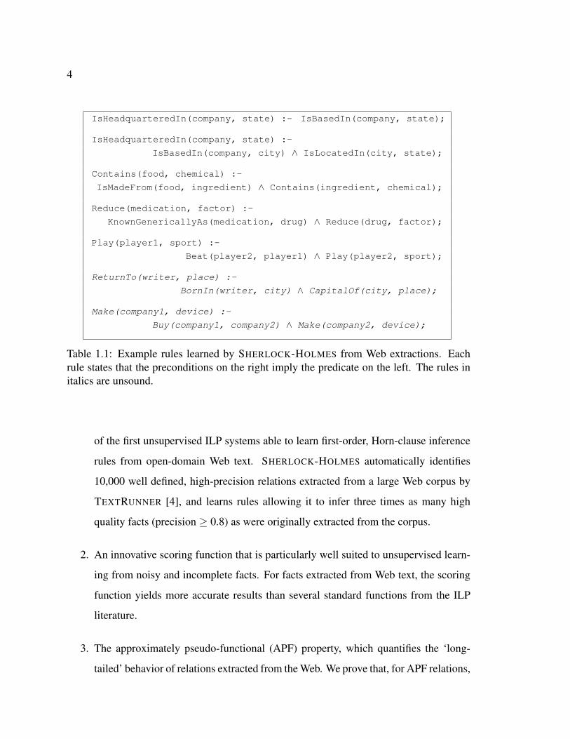
the learned rules to infer answers to queries. Table 1.1 shows some example rules that were
learned by the system. At a high level, SHERLOCK-HOLMES addresses the challenges of
open-domain theories as follows: it handles noise and ambiguity by automatically identi-
fying a clean, well-defined set of facts to learn rules over; it identifies correct rules using
a novel rule-scoring function that is effective for noisy, incomplete, positive-only data; fi-
nally, SHERLOCK-HOLMES operates scalably by exploiting a long-tailed property of facts
on the Web.
The main contributions of this work are as follows:
1. The design, implementation, and evaluation of the SHERLOCK-HOLMES system, one
4
IsHeadquarteredIn(company, state) :- IsBasedIn(company, state);
IsHeadquarteredIn(company, state) :-
IsBasedIn(company, city) ∧ IsLocatedIn(city, state);
Contains(food, chemical) :-
IsMadeFrom(food, ingredient) ∧ Contains(ingredient, chemical);
Reduce(medication, factor) :-
KnownGenericallyAs(medication, drug) ∧ Reduce(drug, factor);
Play(player1, sport) :-
Beat(player2, player1) ∧ Play(player2, sport);
ReturnTo(writer, place) :-
BornIn(writer, city) ∧ CapitalOf(city, place);
Make(company1, device) :-
Buy(company1, company2) ∧ Make(company2, device);
Table 1.1: Example rules learned by SHERLOCK-HOLMES from Web extractions. Eachrule states that the preconditions on the right imply the predicate on the left. The rules initalics are unsound.
of the first unsupervised ILP systems able to learn first-order, Horn-clause inference
rules from open-domain Web text. SHERLOCK-HOLMES automatically identifies
10,000 well defined, high-precision relations extracted from a large Web corpus by
TEXTRUNNER [4], and learns rules allowing it to infer three times as many high
quality facts (precision ≥ 0.8) as were originally extracted from the corpus.
2. An innovative scoring function that is particularly well suited to unsupervised learn-
ing from noisy and incomplete facts. For facts extracted from Web text, the scoring
function yields more accurate results than several standard functions from the ILP
literature.
3. The approximately pseudo-functional (APF) property, which quantifies the ‘long-
tailed’ behavior of relations extracted from the Web. We prove that, for APF relations,

5
SHERLOCK-HOLMES’s runtime will scale linearly in the size of the corpus. We
demonstrate empirically that most relations extracted from the Web are APF, and
furthermore that the runtimes of both rule learning and inference in SHERLOCK-
HOLMES do scale linearly in practice. Therefore, SHERLOCK-HOLMES’s techniques
should be able to operate at Web scale.
4. An extension of SHERLOCK-HOLMES to utilize self-supervised and minimally su-
pervised techniques, and an examination of how they affect the results. We demon-
strate that bootstrapping additional training examples helps the system handle noise
and sparsity better, allowing it to infer many additional facts. Finally, we demonstrate
that a small amount of supervision, in the form of mutual-exclusion constraints on
relations, can improve the system’s precision for those relations.
This dissertation is laid out as follows. We first provide some background definitions
and describe related work in Chapter 2. We then describe the SHERLOCK-HOLMES system
and rule scoring function in Chapter 3, and evaluate them in Chapter 4. Chapter 5 then
introduces the approximately pseudo-functional property, and demonstrates SHERLOCK-
HOLMES’s linear scalability both theoretically and empirically. Chapter 6 examines how
self-supervised and minimally supervised extensions to the system affect its performance.
Finally, we conclude and discuss directions for future research in Chapter 7.
6
Chapter 2
PRIOR WORK
This work builds upon advances in several different subfields of computer science: in-
formation extraction (IE), natural language processing (NLP), inductive logic programming
(ILP), logic, and probabilistic inference. This chapter introduces some definitions, termi-
nology, and background work which are the basis for the SHERLOCK-HOLMES system, and
describes how SHERLOCK-HOLMES fits in with related work in rule learning and inference
in text.
2.1 First-Order Logic
A first-order knowledge base (KB) is a set of formulas in first order logic [23]. The formulas
are constructed using symbols of four types: constants, variables, functions, and predicates.
A constant symbol identifies an object in the domain of interest (e.g., Seattle, Broccoli,
etc.) A variable symbol ranges over objects in the domain. A function symbol maps tuples
of objects to objects in the domain. A predicate symbol represents a relation or property
of a tuple of objects in the domain (e.g., Contains(Broccoli, Calcium)). Constants and
variables may be typed, in which case the constant refers to an object of that type and the
variable may only range over objects of that type.
A term in first-order logic is an expression (constant, variable, or function applied to a
tuple of terms) representing an object in the domain. A ground term is a term containing
no variables. An atom or atomic formula is a predicate symbol applied to a tuple of terms
(e.g., IsBasedIn(x, Seattle)). A ground atom is an atom containing no variables (i.e.,
a predicate symbol applied to a tuple of ground terms). In this work will refer to ground
atoms extracted from the Web as ground facts, but we may alternatively refer to a ground
7
atom as either a ground predicate or a ground relation.
Formulas in first-order logic are constructed recursively from atomic formulas using
logical operators and quantifiers. The logical operators include: ∧ (conjunction, or logical-
and), ∨ (disjuction, or logical-or), ¬ (logical negation), and ⇒ (logical implication). A
literal is an atomic formula (positive literal) or a negation of an atomic formula (negative
literal). A universally quantified formula (∀x F1) is true iff F1 is true for every object x
(possibly typed) in the domain. An existentially quantified formula (∃x F1) is true iff F1 is
true for at least one object x (possibly typed) in the domain.
The formulas in a knowledge base are implicitly conjoined. For automated reasoning,
KBs are typically represented in clausal form (also known as conjunctive normal form).
This format consists of a conjunction of clauses, where each clause is a disjunction of lit-
erals. Every KB in first-order logic can be converted into clausal form using an automated
process. In finite domains, first-order knowledge bases can be propositionalized by replac-
ing an universally quantified formula with a conjunction of all of its groundings, and an
existentially quantified formula with a disjunction of all of its groundings.
A possible world or Herbrand interpretation is an assignment of truth values to all
ground atoms. A formula is satisfiable if there is at least one possible world in which the
formula is true.
Since inference in first-order logic is only semidecidable, we impose some additional
restrictions in this work to make inference tractable. Specifically, we consider a finite,
function-free subset of first-order logic, and we require that all formulas be definite clauses.
A definite clause is a clause containing exactly one positive literal. These clauses corre-
spond to inference rules (logical implications) where the head is a single positive literal,
and the body is a conjunction of positive literals (e.g., the implication P ∧ Q ∧ R ⇒ S
is logically equivalent to the definite clause ¬P ∨ ¬Q ∨ ¬R ∨ S.) Such implications are
also often called Horn clauses. A Horn clause is a clause with at most one positive literal.
Although Horn clauses are a superset of definite clauses, we refer to inference rules in this
work using the terms interchangeably.
8
A relation is said to have closed-world semantics if all ground atoms of that relation
are assumed to be false unless they are explicitly declared to be true in the KB. Otherwise
the relation is said to have open-world semantics. Declaring relations to be closed-world
provides an easy and compact way of restricting the set of possible worlds. As such, many
systems using first-order logic exploit this to improve efficiency. Unfortunately, due to
the sparsity and incompleteness of facts extracted from the Web we can not make this
assumption in this work.
Finally, we say that a clause is connected if the literals in the clause cannot be parti-
tioned into two sets such that the variables appearing in the literals of one set are disjoint
from the variables appearing in the literals of the other set. This essentially says that each
literal in the clause can reach any other literal in the clause via a path of shared variables.
Intuitively, this means that the literals in the clause are all interrelated and affect each other.
In this work, we use the following syntactic conventions when describing objects, rela-
tions, and rules:
1. Constants are written with the first letter in upper-case. When naming a fixed, specific
relation or object, we capitalize words and omit spaces (e.g., we represent the fact that
Seattle is located in Washington as: IsLocatedIn(Seattle, Washington)).
2. Variables are written in lower-case (e.g., IsLocatedIn(x, y)). If there are type re-
strictions on the variable, then for clarity we simply use the type as the name of the
variable (e.g., IsLocatedIn(city, state)).
3. We write rules using a Prolog-like notation, and assume all variables are universally
quantified. For example, we will write the implication P (x, y) ∧ Q(y, z) ⇒ S(x, z)
as S(x, z) : −P (x, y) ∧ Q(y, z);. This rule means: for all values of x, y, and z, if
P (x, y) is true and Q(y, z) is true then S(x, z) is true.
9
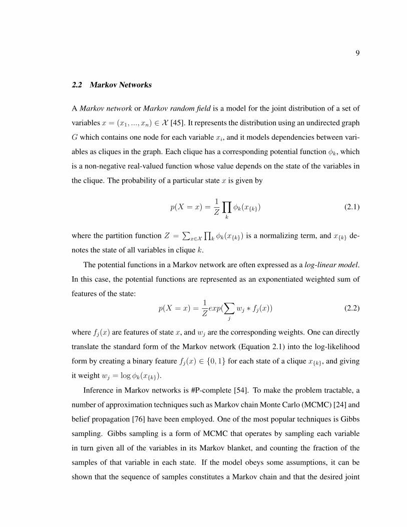
2.2 Markov Networks
A Markov network or Markov random field is a model for the joint distribution of a set of
variables x = (x1, ..., xn) ∈ X [45]. It represents the distribution using an undirected graph
G which contains one node for each variable xi, and it models dependencies between vari-
ables as cliques in the graph. Each clique has a corresponding potential function φk, which
is a non-negative real-valued function whose value depends on the state of the variables in
the clique. The probability of a particular state x is given by
p(X = x) =1
Z
∏k
φk(x{k}) (2.1)
where the partition function Z =∑
x∈X∏
k φk(x{k}) is a normalizing term, and x{k} de-
notes the state of all variables in clique k.
The potential functions in a Markov network are often expressed as a log-linear model.
In this case, the potential functions are represented as an exponentiated weighted sum of
features of the state:
p(X = x) =1
Zexp(
∑j
wj ∗ fj(x)) (2.2)
where fj(x) are features of state x, and wj are the corresponding weights. One can directly
translate the standard form of the Markov network (Equation 2.1) into the log-likelihood
form by creating a binary feature fj(x) ∈ {0, 1} for each state of a clique x{k}, and giving
it weight wj = log φk(x{k}).
Inference in Markov networks is #P-complete [54]. To make the problem tractable, a
number of approximation techniques such as Markov chain Monte Carlo (MCMC) [24] and
belief propagation [76] have been employed. One of the most popular techniques is Gibbs
sampling. Gibbs sampling is a form of MCMC that operates by sampling each variable
in turn given all of the variables in its Markov blanket, and counting the fraction of the
samples of that variable in each state. If the model obeys some assumptions, it can be
shown that the sequence of samples constitutes a Markov chain and that the desired joint
10
distribution is equal to the stationary distribution of that chain [22].
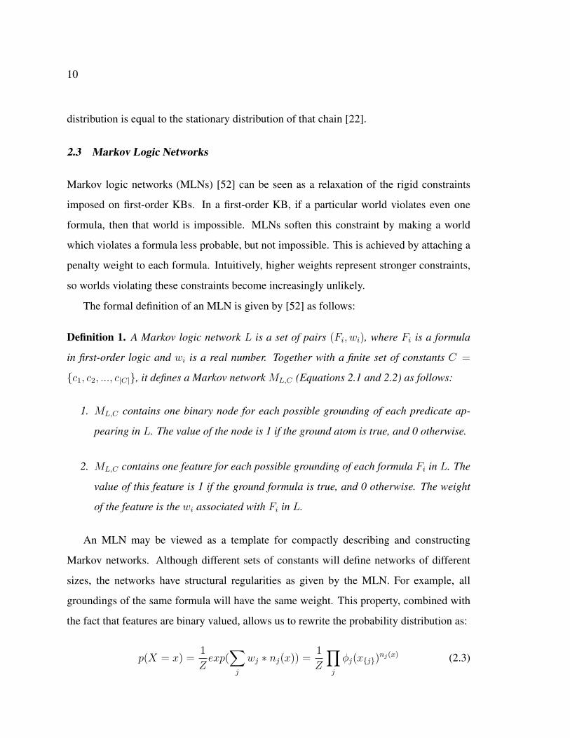
2.3 Markov Logic Networks
Markov logic networks (MLNs) [52] can be seen as a relaxation of the rigid constraints
imposed on first-order KBs. In a first-order KB, if a particular world violates even one
formula, then that world is impossible. MLNs soften this constraint by making a world
which violates a formula less probable, but not impossible. This is achieved by attaching a
penalty weight to each formula. Intuitively, higher weights represent stronger constraints,
so worlds violating these constraints become increasingly unlikely.
The formal definition of an MLN is given by [52] as follows:
Definition 1. A Markov logic network L is a set of pairs (Fi, wi), where Fi is a formula
in first-order logic and wi is a real number. Together with a finite set of constants C =
{c1, c2, ..., c|C|}, it defines a Markov network ML,C (Equations 2.1 and 2.2) as follows:
1. ML,C contains one binary node for each possible grounding of each predicate ap-
pearing in L. The value of the node is 1 if the ground atom is true, and 0 otherwise.
2. ML,C contains one feature for each possible grounding of each formula Fi in L. The
value of this feature is 1 if the ground formula is true, and 0 otherwise. The weight
of the feature is the wi associated with Fi in L.
An MLN may be viewed as a template for compactly describing and constructing
Markov networks. Although different sets of constants will define networks of different
sizes, the networks have structural regularities as given by the MLN. For example, all
groundings of the same formula will have the same weight. This property, combined with
the fact that features are binary valued, allows us to rewrite the probability distribution as:
p(X = x) =1
Zexp(
∑j
wj ∗ nj(x)) =1
Z
∏j
φj(x{j})nj(x) (2.3)
11
where nj(x) is the number of true groundings of Fj in x, x{j} is the truth values of the
atoms appearing in Fj , and φj(x{j}) = ewj
The SHERLOCK-HOLMES system described in Chapter 3 uses techniques of the MLN
framework as a way of modeling uncertainty in extractions and inferences.
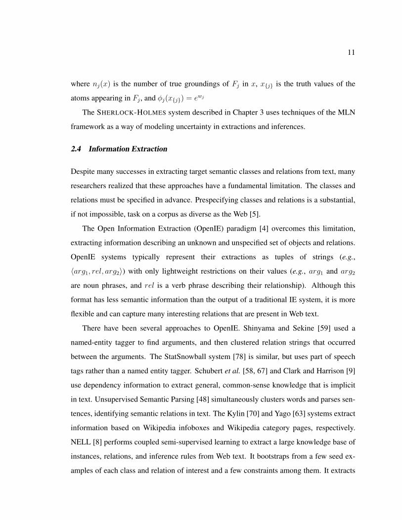
2.4 Information Extraction
Despite many successes in extracting target semantic classes and relations from text, many
researchers realized that these approaches have a fundamental limitation. The classes and
relations must be specified in advance. Prespecifying classes and relations is a substantial,
if not impossible, task on a corpus as diverse as the Web [5].
The Open Information Extraction (OpenIE) paradigm [4] overcomes this limitation,
extracting information describing an unknown and unspecified set of objects and relations.
OpenIE systems typically represent their extractions as tuples of strings (e.g.,
〈arg1, rel, arg2〉) with only lightweight restrictions on their values (e.g., arg1 and arg2
are noun phrases, and rel is a verb phrase describing their relationship). Although this
format has less semantic information than the output of a traditional IE system, it is more
flexible and can capture many interesting relations that are present in Web text.
There have been several approaches to OpenIE. Shinyama and Sekine [59] used a
named-entity tagger to find arguments, and then clustered relation strings that occurred
between the arguments. The StatSnowball system [78] is similar, but uses part of speech
tags rather than a named entity tagger. Schubert et al. [58, 67] and Clark and Harrison [9]
use dependency information to extract general, common-sense knowledge that is implicit
in text. Unsupervised Semantic Parsing [48] simultaneously clusters words and parses sen-
tences, identifying semantic relations in text. The Kylin [70] and Yago [63] systems extract
information based on Wikipedia infoboxes and Wikipedia category pages, respectively.
NELL [8] performs coupled semi-supervised learning to extract a large knowledge base of
instances, relations, and inference rules from Web text. It bootstraps from a few seed ex-
amples of each class and relation of interest and a few constraints among them. It extracts
12
additional facts from Web pages using a variety of techniques (e.g., learned extraction pat-
terns, wrapper induction, and learned inference rules). Finally, the TEXTRUNNER [4] and
WOE [71] systems extract relational triples from arbitrary sentences using a conditional
random field and part-of-speech tags or parse features.
Although this work uses TEXTRUNNER’s extractions as its knowledge base, the meth-
ods presented are more general. TEXTRUNNER’s extractions take the form of simple tex-
tual triples 〈arg1, rel, arg2〉, where arg1 and arg2 are noun phrases, and rel is a string
representing the relation between the two arguments. We treat the extractions as first-order,
ground atoms of the form rel(arg1, arg2), but call them extracted facts to reinforce that
rel, arg1, and arg2 are noisy, ambiguous, and arbitrary strings extracted by TEXTRUN-
NER, and not the clean, well-defined, and uniquely named objects and relations typically
used in first-order KBs. To give a sense of scale, TEXTRUNNER extracted 800 million such
facts from over 500 million high quality Web pages. While this is only a small fraction of
the Web, it approximates the large scale behavior of relations in Web text.
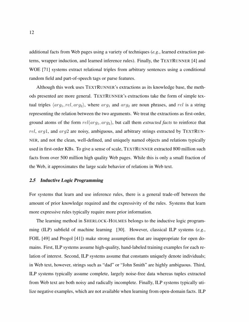
2.5 Inductive Logic Programming
For systems that learn and use inference rules, there is a general trade-off between the
amount of prior knowledge required and the expressivity of the rules. Systems that learn
more expressive rules typically require more prior information.
The learning method in SHERLOCK-HOLMES belongs to the inductive logic program-
ming (ILP) subfield of machine learning [30]. However, classical ILP systems (e.g.,
FOIL [49] and Progol [41]) make strong assumptions that are inappropriate for open do-
mains. First, ILP systems assume high-quality, hand-labeled training examples for each re-
lation of interest. Second, ILP systems assume that constants uniquely denote individuals;
in Web text, however, strings such as “dad” or “John Smith” are highly ambiguous. Third,
ILP systems typically assume complete, largely noise-free data whereas tuples extracted
from Web text are both noisy and radically incomplete. Finally, ILP systems typically uti-
lize negative examples, which are not available when learning from open-domain facts. ILP
13
systems, and the Markov logic structure learning systems that are their probabilistic coun-
terparts (e.g., [28, 27]), require training data and relatively clean background knowledge.
They are not designed to handle the noise and incompleteness of open-domain, extracted
facts.
A few systems have tried to relax some of these requirements. Claudien [15] and Ter-
tius [20] are unsupervised ILP systems which learn rules from a database of ground rela-
tions. These systems look for statistical regularities in the database and create inference
rules capturing those regularities. Muggleton [42] extended the Progol ILP system to learn
inference rules from only positive examples, but his results depend on noise-free training
data. The LIME ILP system [37] derived more general results that account for random
errors in the training data. Unfortunately, all of these systems require completely specified,
noise-free background data and domain specific priors describing how likely an inference
rule is to be true. These assumptions are not valid for Web extractions, which are noisy, am-
biguous, and incomplete. We compare SHERLOCK-HOLMES’s rule scoring function with
LIME’s in Section 4.2.
ILP has also been used for information extraction on the Web. Craven et al.[11] used
ILP to help extract information from Web pages, but required training examples and fo-
cused on a single domain. More recently, the NELL system [8] has learned inference
rules over a larger number of relations extracted from the Web. For accuracy, inference
rules must be validated by a human before being used by NELL. In contrast, SHERLOCK-
HOLMES focuses mainly on learning inference rules and using them to answer queries, but
does not require any manually validated rules, seeds, or constraints.
2.6 Textual Inference
Two other notable systems that learn inference rules from text are DIRT [32] and RE-
SOLVER [75]. DIRT and RESOLVER are unsupervised, open-domain systems that learn a
set of rules capturing synonyms, paraphrases, and simple entailments. For example, these
systems may learn the rule x Acquired y =⇒ x Bought y, which captures different ways
14
of describing a purchase. Applications of these rules often depend on context (e.g., if a per-
son acquires a skill, that does not mean they bought the skill). To add the necessary context,
the ISP [44] system learned selectional preferences [51] for DIRT’s rules. The selectional
preferences act as type restrictions on the arguments, and attempt to filter out incorrect in-
ferences. However, these systems only consider rules with one relation in the body. They
do not learn more expressive, multi-part Horn-clauses. As such, the rules learned by these
approaches are useful, but they are strictly more limited than the rules learned and used by
SHERLOCK-HOLMES.
The Recognizing Textual Entailment (RTE) task [13] is to determine whether one short
text (typically a sentence or two) entails another. Approaches to RTE include those of Tatu
and Moldovan [64], which generated inference rules from WordNet lexical chains and a
set of axiom templates, and Pennacchiotti and Zanzotto [47], which learned inference rules
based on similarity across entailment pairs. In contrast with SHERLOCK-HOLMES, RTE
systems reason over full sentences, but benefit from being given a limited set of sentences
to consider. RTE systems may ignore all other text. SHERLOCK-HOLMES operates over
simpler facts extracted from Web text, but is not given guidance as to which facts may
interact.
2.7 Association Rule Mining
Other work on unsupervised rule learning in large databases includes association rule min-
ing [2, 3]. The association rule mining task is to find rules predicting what items frequently
appear together in a database of transactions. For instance, when looking at grocery store
purchases, it is interesting to know that if a person buys milk and bread then they are likely
to also purchase butter. The rules are typically required to have some minimum support
(observed frequency in the database), as well as some minimum confidence (conditional
probability). Although SHERLOCK-HOLMES uses similar concepts when learning rules,
there are a number of important distinctions. Firstly, the database schema is well-defined
in association rule mining, whereas the objects and relations described in facts extracted
15
from the Web are arbitrary strings. Secondly, the database in association rule mining is
complete and noise free, whereas facts extracted from the Web are both noisy and radically
incomplete. As such, SHERLOCK-HOLMES must use different methods for creating and
evaluating the rules.
2.8 Learning from Only Positive Examples
Elkan and Noto [17] considered the problem of learning a classifier from only positive and
unlabeled data. In the noise free case, they proved that probabilities predicted by a classifier
in this setting differ from the true probabilities by only a constant factor. However, their
results are defined in a propositional setting, where they can assume that examples are
independent and identically distributed (IID).
Yu, Han, and Chang introduced the PEBL framework [77] for classifying web pages
using only positive and unlabeled examples. To do so, they initialize a set of negative
examples as the unlabeled examples that are furthest from positive examples. They then
train an SVM to recognize the negative examples, and iteratively expand the set of negative
examples using the SVM’s classifications. The net effect is that, at each iteration, the SVM
gets closer to the true decision boundary. They demonstrated that this technique yielded
results comparable to learning a classifier using positive and negative labeled data.
Unfortunately, both of these systems assume that examples are IID and have a large
number of features. These assumptions are not valid for the facts extracted from Web text
by TEXTRUNNER. Specifically, popular entities are much more likely to appear in TEX-
TRUNNER’s extractions, since they are mentioned more frequently in Web text. The flip
side of this is that TEXTRUNNER is much more likely to be missing information about rare
entities, and so we are disproportionally less likely to infer facts about rare entities. Addi-
tionally, TEXTRUNNER makes some systematic extraction errors. These errors will be cor-
related, violating the assumption that these ‘observed’ examples are IID. Finally, the facts
extracted by TEXTRUNNER are simple textual relations, not full textual documents. As
such, we have less contextual information than these prior, positive-only learning-systems.

16
Chapter 3
SHERLOCK-HOLMES SYSTEM DESIGN
The goal of the SHERLOCK-HOLMES system is to learn inference rules from open-
domain Web text, and then to use those rules to help answer queries. SHERLOCK-HOLMES
is one of the first unsupervised, open-domain systems capable of going beyond simple
paraphrase rules to learn complex, multi-part inference rules from Web text. These rules
enable the system to infer answers to queries even when the answers are not stated on
any single page in the corpus. This chapter describes how SHERLOCK-HOLMES learns
inference rules and uses them to answer queries.
3.1 System Overview
The SHERLOCK-HOLMES system consists of two components: SHERLOCK [56], which
learns inference rules offline, and HOLMES [57], which uses inference rules to answer
queries online. The architecture of SHERLOCK-HOLMES is depicted in Figure 3.1.
SHERLOCK takes as input a large set of open-domain facts, and returns a set of weighted,
first-order, Horn-clause inference rules. These rules take the form
Head(v1, v2) : −Body1(v11, v12) ∧ ... ∧ Bodyk(vk1, vk2);
where Head and Bodyi are function-free, non-negated, first-order relations.1 This rule
means that if Body1(v11, v12) ∧ ... ∧ Bodyk(vk1, vk2) is true, then Head(v1, v2) is true. Ta-
ble 1.1 in the introduction previously showed some example rules which were learned by
SHERLOCK.
1For simplicity we show only relations with two arguments, but the techniques presented are more general.
17
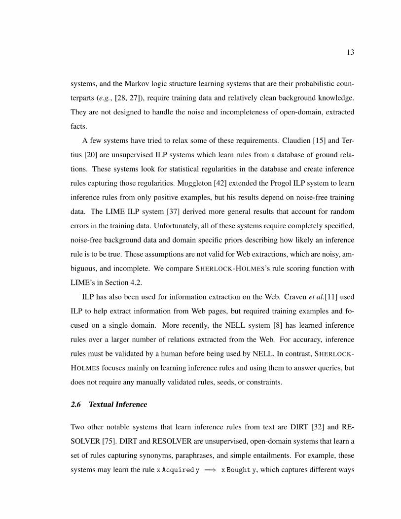
Figure 3.1: Architecture of the SHERLOCK-HOLMES system. SHERLOCK learns inferencerules offline and provides them to the HOLMES inference engine, which uses the rules toanswer queries online.
In order to learn inference rules, SHERLOCK performs the following steps:
1. Identify a “productive” set of classes and instances of those classes
2. Discover relations between classes
3. Learn inference rules using the discovered relations
4. Determine the confidence in each rule
Steps 1 and 2 combat the challenges of synonyms, homonyms, and noise present in open-
domain theories by identifying a smaller, cleaner, and more cohesive set of facts to learn
rules over. These learned rules are then used by HOLMES to answer queries.
HOLMES takes as input a set of open-domain facts, weighted Horn-clause inference
rules, and a conjunctive query. To answer the query it performs a form of Knowledge
Based Model Construction [69], first finding candidate answers using logical inference,
18
kaleprevents
osteoporosis(Inferred : 0.66)
broccoliis high incalcium
(TextRunner : 0.29)
kaleis high in
magnesium(TextRunner : 0.29)
kaleis high incalcium
(TextRunner : 0.42)
magnesiumprevents
osteoporosis(TextRunner : 0.29)
calciumprevents
osteoporosis(TextRunner : 0.51)
broccoliprevents
osteoporosis(Inferred : 0.37)
kaleIS-A
vegetable(TextRunner : 0.75)
kale matches the query(Inferred : 0.68)
Inf. Rule:Transitive-Through
high in
Inf. Rule:Transitive-Through
high in
Query Result
broccoliIS-A
vegetable(TextRunner : 0.75)
broccoli matches the query(Inferred : 0.44)
Query Result
Inf. Rule:Transitive-Through
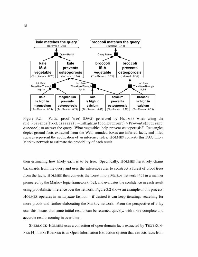
high in
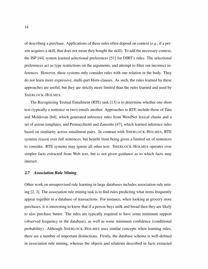
Figure 3.2: Partial proof ‘tree’ (DAG) generated by HOLMES when using therule Prevents(food, disease) : −IsHighIn(food, nutrient) ∧ Prevents(nutrient,disease); to answer the query ‘What vegetables help prevent osteoporosis?’ Rectanglesdepict ground facts extracted from the Web, rounded boxes are inferred facts, and filledsquares represent the application of an inference rules. HOLMES converts this DAG into aMarkov network to estimate the probability of each result.
then estimating how likely each is to be true. Specifically, HOLMES iteratively chains
backwards from the query and uses the inference rules to construct a forest of proof trees
from the facts. HOLMES then converts the forest into a Markov network [45] in a manner
pioneered by the Markov logic framework [52], and evaluates the confidence in each result
using probabilistic inference over the network. Figure 3.2 shows an example of this process.
HOLMES operates in an anytime fashion – if desired it can keep iterating: searching for
more proofs and further elaborating the Markov network. From the perspective of a lay
user this means that some initial results can be returned quickly, with more complete and
accurate results coming in over time.
SHERLOCK-HOLMES uses a collection of open-domain facts extracted by TEXTRUN-
NER [4]. TEXTRUNNER is an Open Information Extraction system that extracts facts from
19
Web pages in a domain independent way. The extracted facts represent simple textual
relations of the form r(x, y) where x and y are strings referring to entities and r is a
string describing the relation between them. For example, TEXTRUNNER extracts the facts
Contains(Broccoli, Calcium), IsLocatedIn(Seattle, Washington), and
Acquired(Google, YouTube).
Unfortunately, sentences on the Web rarely describe when a relation does not hold; for
example, we are unlikely to see a sentence explicitly declaring that ‘Seattle is not located in
Arizona’ (Not(IsLocatedIn(Seattle, Arizona)). The facts extracted by TEXTRUNNER
are positive instances of relations, and TEXTRUNNER does not provide reliable negative
facts. Furthermore, we cannot make the closed-world assumption or even assume that re-
lations are mutually exclusive, since many facts are never explicitly stated and many of
the extracted relations are similar (e.g., IsTheCapitalOf and IsLocatedIn). Finally,
SHERLOCK-HOLMES’s focus is on rule learning and inference within open-domain theo-
ries, and so it delegates syntactic problems (e.g., anaphora, relative clauses) and semantic
challenges (e.g., quantification, counterfactuals, temporal qualification) to the extraction
system or simply ignores them. SHERLOCK-HOLMES’s methods therefore are geared to-
wards learning rules in the presence of positive-only, noisy, and radically-incomplete data
as is found on the Web.
Although SHERLOCK-HOLMES currently uses the facts extracted by TEXTRUNNER,
the techniques presented are more broadly applicable. The next sections describe
SHERLOCK-HOLMES’s design in more detail.
3.2 Finding Classes and Instances
As its first step, SHERLOCK searches for a set of well-defined classes and class instances.
Instances of the same class should tend to behave similarly, so identifying a good set of
instances will make it easier to discover the general properties of the entire class.
Options for identifying interesting classes include manually created methods (e.g., Word-
Net [39]), textual patterns [25], automated clustering [33], and combinations of all three [61].
20
SHERLOCK identifies classes and instances using the Hearst patterns [25] (e.g., ‘Class such
as Instance’), because the patterns are simple, capture how classes and instances are men-
tioned in Web text, and yield intuitive, explainable groups. Using these patterns, 29 million
(instance, class) pairs were extracted from a large Web crawl. They were then cleaned
using word stemming, normalization, and by dropping modifiers.
Unfortunately, the Hearst patterns make systematic errors (e.g., extracting ‘Canada’ as
the name of a city from the phrase ‘Toronto, Canada and other cities.’) To address this issue,
SHERLOCK discards the low frequency classes of each instance. This heuristic reduces
the noise due to systematic error while still capturing the important senses of each word.
Additionally, the extraction frequency is used to estimate the probability that a particular
mention of an instance refers to each of its potential classes (e.g., New York appears as a
city 40% of the time, a state 35% of the time, and a place, area, or center the remaining
25% of the time).
Ambiguity presents a significant obstacle when learning inference rules. For example,
the corpus contains the sentences ‘broccoli contains this vitamin’ and ‘this vitamin prevents
scurvy’, but it is unclear if the sentences refer to the same vitamin. To address this, we elim-
inate ambiguous instances and only retain facts with unambiguous arguments. We observed
two main sources of ambiguity: references to a more general class instead of a specific in-
stance (e.g., the string ‘vitamin’ is often extracted as an instance of the ‘nutrient’ class),
and references to a person by only their first or last name (e.g., ‘Jane’ or ‘Smith’). SHER-
LOCK eliminates the first case by removing terms that frequently appear as the class name
with other instances (e.g., the string ‘vitamin’ is ambiguous since it frequently appears as
a class name with instances such as ‘vitamin c’, ‘folic acid’, etc.). SHERLOCK eliminates
the second case by removing the 2,500 most common first and last names, according to the
US Census Bureau.2
After eliminating ambiguous instances, we identify a set of common, well-defined
2http://www.census.gov/genealogy/names/names_files.html
21
classes. The 250 most frequently mentioned class names include a large number of in-
teresting classes (e.g., companies, cities, foods, nutrients, locations) and some ambiguous
concepts (e.g., ideas, things.) SHERLOCK focuses on the less ambiguous classes by elim-
inating any class not appearing as a descendant of physical entity, social group, physical
condition, or event in WordNet. Beyond this filtering, classes are treated independently and
no use of a type hierarchy is made.
This process identifies 1.1 million distinct, cleaned (instance, class) pairs for 156 classes.
A complete listing of the classes is given in Appendix B.
3.3 Discovering Relations between Classes
Next, SHERLOCK discovers how classes relate to and interact with each other. Prior work
in relation discovery [59] has investigated the problem of finding relationships between dif-
ferent classes. However, since SHERLOCK’s focus is on rule-learning and not on relation-
discovery, the system uses a few simple heuristics to automatically identify interesting re-
lations.
For every pair of classes (C1, C2), SHERLOCK finds a set of typed, candidate relations
from the 100 most frequent relations in the corpus where the first argument is an instance
of C1 and the second argument is an instance of C2. For terms with multiple senses (e.g.,
New York), their weights are split based on how frequently they appear with each class in
the Hearst patterns.
However, many discovered relations are incorrect or meaningless, arising from either
extraction errors or word-sense ambiguity. For example, the extracted fact
IsBasedIn(Apple, Cupertino) gives some evidence that a fruit may possibly be based
in a city. These incorrectly-typed relations are filtered using two heuristics. First, any re-
lation whose weighted frequency falls below a threshold is discarded, since rare relations
are more likely to arise due to extraction errors or word-sense ambiguity. Additionally,
relations whose pointwise mutual information (PMI) is below a threshold T=exp(2) ≈ 7.4
22
are also removed. A relation’s PMI is:
PMI(R(C1, C2)) =p(R,C1, C2)
p(R, ·, ·) ∗ p(·, C1, ·) ∗ p(·, ·, C2)(3.1)
where p(R, ·, ·) is the probability a random fact has relation R, p(·, C1, ·) is the probability
a random fact has an instance of C1 as its first argument, p(·, ·, C2) is the probability a ran-
dom fact has an instance of C2 as its second argument, and p(R,C1, C2) is the probability
that a random fact has relation R and instances of C1 and C2 as its first and second argu-
ments, respectively. A low PMI indicates the relation occurred by random chance, which is
typically due to ambiguous terms or extraction errors.
Finally, two TEXTRUNNER specific cleaning heuristics are used: a small set of stop-
relations (‘be’, ‘have’, and ‘be preposition’) are ignored, and extracted facts whose argu-
ments are more than four tokens apart are discarded. This process identifies over 10,000
typed relations from the facts extracted by TEXTRUNNER. We note that, although there is
some overlap in relations with related types (e.g., IsBasedIn(company, city) vs.
IsBasedIn(company, place)), this overlap will implicitly allow the system to learn rules
at different granularities. A complete listing of the relations is available on the Web. See
Appendix A for details.
3.4 Learning Inference Rules
SHERLOCK attempts to learn inference rules for each typed relation in turn. It receives a
target relation, R, a set of observed examples of the relation, E+, a maximum clause length
k, a minimum support, s, and an acceptance threshold, t, as input. SHERLOCK generates
inference rules for R by constructing all first-order, definite clauses up to length k, where R
appears as the head of the clause (i.e., all rules of the form R(...):-B1(...) ∧ ... ∧ Bn(...); for
1 ≤ n ≤ k). We accept all rules that obey the following constraints:
1. Contains no unbound variables
23
2. Has a connected rule body
3. Infers at least s examples from E+
4. Scores at least t according to the score function
The next section describes the score function SHERLOCK uses to evaluate rules, and Sec-
tion 4.2 validates it empirically.
3.5 Evaluating Rules by Statistical Relevance
The problem of evaluating candidate rules has been studied by many researchers, but typ-
ically in either a supervised or propositional context. However, SHERLOCK’s goal is to
learn first-order Horn-clauses from an unsupervised, noisy, positive-only set of facts ex-
tracted from Web text. Moreover, due to the incomplete nature of the input corpus and the
imperfect yield of extraction—many true facts are not stated explicitly in the set of ground
facts used by the learner to evaluate rules.
The absence of negative examples, coupled with noise and incomplete data, means
that standard ILP evaluation functions (e.g., information gain [49] or the M-Estimate rule
scoring function [16]) are not appropriate. Furthermore, when evaluating a particular rule
Head:-Body, it is natural to consider p(Head|Body) but, due to missing data, this absolute
probability estimate is often misleading: in many cases Head will hold given Body but the
Head is not explicitly mentioned in the corpus.
To address this problem when evaluating propositional rules, Salmon et al. [55] pro-
posed using relative probability estimates. I.e., is p(Head|Body) � p(Head)? If so, then
Body is said to be statistically relevant to Head. At a high level, statistical relevance tries to
infer the simplest set of factors which explain an observation. It can be viewed as searching
for the simplest propositional Horn-clause which increases the likelihood of a goal propo-
sition g. The two key ideas in determining statistical relevance are (1) discovering factors
24
which substantially increase the likelihood of g (even if the probabilities are small in an
absolute sense), and (2) dismissing irrelevant factors.
To illustrate these concepts, consider the following example. Suppose our goal is to
predict if New York City will have a storm (S). On an arbitrary day, the probability of
having a storm is fairly low (p(S) � 1). However, if we know that the atmospheric pres-
sure on that day is low, this substantially increases the probability of having a storm (al-
though that probability may still be small in an absolute sense). According to the principle
of statistical relevance, low atmospheric pressure (LP ) is a factor which predicts storms
(S : −LP ), since p(S|LP )� p(S).
The principle of statistical relevance also identifies and removes irrelevant factors. For
example, let M denote the gender of New York’s mayor. Since p(S|LP,M) � p(S), it
naıvely appears that storms in New York depend on the gender of the mayor in addition
to the air pressure. The statistical relevance principle sidesteps this trap by removing any
factors which are conditionally independent of the goal, given the remaining factors. In
this example we would observe that p(S|LP )=p(S|LP,M), and so we say that M is not
statistically relevant to S. This test applies Occam’s razor by searching for the simplest rule
which explains the goal.
Statistical relevance is useful in an open-domain setting, since all the necessary proba-
bilities can be estimated from only positive examples. Furthermore, approximating relative
probabilities in the presence of missing data is much more reliable than determining abso-
lute probabilities.
Unfortunately, Salmon et al. [55] defined statistical relevance in a propositional con-
text. One technical contribution of our work is to lift statistical relevance to first-order
Horn-clauses as follows. For the Horn-clause Head(v1, ..., vn):-Body(v1, ..., vm) (where
Body(v1, ..., vm) is a conjunction of function-free, non-negated, first-order relations, and
vi ∈ V is the set of typed variables used in the rule), the Body helps explain the Head if:
1. Observing a grounding of Body(v1, ..., vm) substantially increases the probability of
25
observing the corresponding ground instance of Head(v1, ..., vn).
2. Body(v1, ..., vm) contains no irrelevant (conditionally independent) terms.
Conditional independence of terms is evaluated using ILP’s technique of Θ-subsumption,
ensuring there is no more general clause that is similarly predictive of the head. For-
mally, clause C1 Θ-subsumes clause C2 if and only if there exists a substitution Θ such
that C1Θ ⊆ C2 where each clause is treated as the set of its literals. For example, R(x, y)
Θ-subsumes R(x, x), since {R(x, y)}Θ ⊆ {R(x, x)} when Θ={y/x}. Intuitively, if C1 Θ-
subsumes C2, it means that C1 is more general than C2.
Definition 2. A first-order Horn-clause Head(...):-Body(...) is statistically relevant if
p(Head(...)|Body(...)) � p(Head(...)) and if there is no clause body B′(...)Θ ⊆ Body(...)
such that p(Head(...)|Body(...)) ≈ p(Head(...)|B′(...)).
In practice it is difficult to determine the probabilities exactly, so when checking for
statistical relevance the system ensures that the probability of the rule is at least a factor
t greater than the probability of any subsuming rule, that is, p(Head(...)|Body(...)) ≥ t ∗
p(Head(...)|B′(...)). We use this value of t as the statistical relevance score.
For all values of B(...), the probability p(Head(...)|B(...)) is estimated from the observed
facts by assuming values of Head(...) are generated by sampling values of B(...) as follows:
for variables vs shared between Head(...) and B(...), values of vs are sampled uniformly
from all observed groundings of B(...). For variables vi, if any, that appear in Head(...)
but not in B(...), their values are sampled according to a distribution p(vi|classi). The
distribution p(vi|classi) is approximated using the relative frequency that vi was extracted
using a Hearst pattern with classi.
Finally, the increase in likelihood must be statistically significant. This is tested using
the likelihood ratio statistic:
2Nr
∑H(...)∈{Head(...),¬Head(...)}
p(H(...)|Body(...)) ∗ logp(H(...)|Body(...))
p(H(...)|B′(...))(3.2)
26
where p(¬Head(...)|B(...)) = 1−p(Head(...)|B(...)) andNr is the number of results inferred
by the rule Head(...):-Body(...). This test is distributed approximately as χ2 with one degree
of freedom. It is similar to the statistical significance test used in mFOIL [16], but has two
modifications since SHERLOCK does not have labeled training data. In lieu of positive
and negative examples, the system uses whether or not the inferred value of Head(...) was
observed, and compares against the distribution of a subsuming clause B′(...) rather than a
known prior.
This method of evaluating rules has two important differences from ILP under a closed-
world assumption. First, these probability estimates consider the fact that examples pro-
vide varying amounts of information. Second, statistical relevance finds rules with large
increases in relative probability, not necessarily a large absolute probability. This is cru-
cial in an open-domain setting where most facts are false, which means the trivial rule that
everything is false will have high accuracy. Even for true rules, the observed estimates
p(Head(...)|Body(...))� 1 due to missing data and noise.
3.6 Making Inferences
The rules learned by SHERLOCK are provided to the HOLMES inference engine. As input,
HOLMES requires a conjunctive query Q, an evidence set E and set of weighted rules R.
It performs a form of knowledge based model construction [69], first finding facts using
logical inference, then estimating the confidence of each fact using a Markov logic network
(MLN) [52].
Prior to running inference, it is necessary to assign a weight to each rule learned by
SHERLOCK. Since the rules and inferences are based on a set of noisy and incomplete
extractions, the algorithms used for both weight learning and inference should capture the
following characteristics of facts extracted from the Web:
C1. Any arbitrary unknown fact is highly unlikely to be true.
27
C2. The more frequently a fact is extracted from the Web, the more likely it is to be true.
However, facts in E should have a confidence bounded by a threshold, pmax, such
that pmax < 1. E contains systematic extraction errors, so uncertainty is a desired
trait in even the most frequently extracted facts.
C3. An inference that combines uncertain facts should be less likely than each fact it uses.
Next, the modifications to the weight learning and inference algorithm needed to achieve
the desired behavior are described.
3.6.1 Weight Learning
SHERLOCK uses the discriminative weight learning procedure described by Huynh and
Mooney [27]. This weight learning method is efficient since it avoids computing the parti-
tion function by computing probabilities in closed form. However, to do so it assumes that
(1) all rules infer a single head predicate, (2) all other predicates are evidence, and (3) all
ground atoms of the target predicate are conditionally independent, given the evidence. As
a consequence of these assumptions, this method does not allow recursive rules. This is a
substantial limitation on expressivity, but it enables efficient probabilistic inference.
To meet the assumptions we only allow inferences of depth one (i.e., we do not con-
sider inference chains over multiple rules,) and introduce the following modifications to
help account for noise. Deeper inferences over noisy extractions tend to be much more
error prone, so in practice these limitations reduces recall, but substantially improves both
precision and computational efficiency.
Learning the weights involves counting the number of true groundings for each rule in
the data [52]. However, the noisy nature of Web extractions will make this count an over-
estimate. Consequently, ni(E), the number of true groundings of rule i from Equation 2.3,
28
is computed as follows:
ni(E) =∑
j
maxk
∏B(...)∈Bodyijk
p(B(...)) (3.3)
where E is the evidence, j ranges over the observed values of the head of the rule, Bodyijk
is the body of the kth grounding for the jth head of rule i, and p(B(...)) is approximated
using a logistic function of the number of times B(...) was extracted,3 scaled to be in
the range [0, 0.75]. This models C2 by giving increasing but bounded confidence for
more frequently extracted facts. In practice, this also helps address C3 by giving longer
rules smaller values of ni, which reflects that inferences arrived at through a combination
of multiple, noisy facts should have lower confidence. Longer rules are also more likely
to have multiple groundings that infer a particular head, so keeping only the most likely
grounding prevents a head from receiving undue weight from any single rule.
Finally, SHERLOCK places a very strong Gaussian prior (i.e., L2 penalty) on the weights.
Longer rules have a higher prior to capture the notion that they are more likely to make in-
correct inferences. Without a high prior, each rule would receive an unduly high weight as
there are no negative examples available.
3.6.2 Probabilistic Inference
After learning the weights, the following two rules are added to the rule set:
1. H(...) with negative weight wprior
2. H(...):-ExtractedFrom(H(...),sentencei) with weight 1
The first rule models C1 by saying that most facts are false. The second rule models C2
by stating that the probability of a fact depends on the number of times it was extracted.
The weights of these rules are fixed. These rules are not included during weight learning as
3This approximation is equivalent to an MLN which uses only the two rules defined in 3.6.2
29
doing so swamps the effects of the other inference rules (i.e., forces their weights to zero).
HOLMES’s probabilistic inference also requires computing ni(E); this is done according to
Equation 3.3 as in weight learning.
We limit HOLMES’s inferences to depth one so that it meets the assumptions needed for
weight learning and for computing the probabilities in closed form. However, if desired,
the HOLMES inference engine can perform anytime, incremental inference. As time allows,
it augments the Markov network with deeper and deeper inferences, and uses a form of
loopy belief propagation [45] to estimate the probabilities of each of its inferred facts. The
experiments in [57] take advantage of this ability, but for efficiency the experiments in
Chapters 4-6 used the depth-limited, closed-form method as described above.
30
Chapter 4
EVALUATION OF THE SHERLOCK-HOLMES SYSTEM
This chapter demonstrates the utility of the SHERLOCK-HOLMES system empirically.
There are two ways of evaluating a rule learner: directly estimating the quality of the
learned rules, or measuring the impact of the rules on a system that uses them. Since
the notion of ‘rule quality’ is vague outside the context of an application, we evaluate
SHERLOCK-HOLMES in the context of the an inference-based question answering system.
One of the primary goals of the SHERLOCK-HOLMES system is to better answer com-
plex queries such as ‘What foods prevent disease?’, where the information needed to com-
pute the answers may be spread over multiple pages. Therefore, our evaluation focuses on
the task of computing as many instances as possible of an atomic pattern Rel(x, y). In this
example, Rel would be bound to ‘Prevents’, x would have type ‘Food’ and y would have
type ‘Disease.’
But which relations should be used in the test? There is a large variance in behavior
across relations, so examining any particular relation may give misleading results. Instead,
these experiments examine the global performance of the system by querying HOLMES for
all open-domain relations identified in Section 3.3 as follows:
1. Score all candidate rules according to the rule scoring metric M , accept all rules
with a score at least tM , and learn weights for all accepted rules. tM was tuned to
maximize the F1 measure over a small development set of rules, which was created
by sampling approximately 700 rules (of the 4.9M candidate rules which had some
minimum support), and then manually judging whether the rule was correct or not.
2. Find all facts inferred by the rules and estimate their probabilities using the rule
31
weights.
3. Reduce type information. For each fact, (e.g., IsBasedIn(Diebold, Ohio)) which
has been deduced with multiple type signatures (e.g., Ohio is both a state and a geo-
graphic location), keep only the one with maximum probability (i.e., conservatively
assuming dependence).
4. Estimate the precision and number of inferred facts that are correct (relative recall)
in the results. This is done by placing all inferred facts into bins based on their
probabilities and estimating the precision and relative recall of the bin by manually
evaluating 50 randomly sampled facts from the bin.
Since TEXTRUNNER [4] does not extract temporal information, we judge an inferred
fact as correct if it was true at any point in time (e.g., both IsBasedIn(Boeing, Seattle)
and IsBasedIn(Boeing, Chicago) would be considered true, since Boeing moved its com-
pany headquarters from Seattle to Chicago in 2001). Additionally, we estimate the relative
recall (number of correct facts) instead of true recall since most of these relations have no
exhaustive ground truth to compare against.
These experiments consider rules with up to k = 2 relations in the body. Although this
number may seem small, learning rules with multiple relations in the body represents an
important leap beyond previous open-domain rule-learning systems. Previous systems such
DIRT [32] and RESOLVER [75] only consider rules with one relation in the body, and so
can only infer paraphrases of other directly stated facts. These systems are helpless if two
entities are not mentioned in the same sentence. By considering rules with two relations in
the body, SHERLOCK can overcome this limitation. The rules learned by SHERLOCK can
combine facts extracted from multiple pages to infer results not stated in any form within
the corpus.
These experiments use a corpus of 1 million raw extractions, corresponding to 250,000
distinct facts. The facts represent a wide variety of domains, covering a total of 10,672
32
typed relations. There are between a dozen and 2,375 ground facts observed for each
typed relation. Out of 110 million possible rules satisfying type constraints, SHERLOCK-
HOLMES found 5 million candidate rules that infer at least two of the observed facts. Un-
less otherwise noted, SHERLOCK’s rule scoring function is used to evaluate the rules (as
described in Section 3.5). Learning all rules, rule weights, and inferring all the results took
approximately 50 minutes when coarsely parallelized on a cluster with 72 cores.Each node
in our cluster had two mutlti-threaded, 2.8 GHz Intel Xeon processor cores and a total of
4GB system memory. The runtime could be improved with additional engineering efforts,
but was fast enough for our purposes. The rules learned by SHERLOCK are available on the
Web. See Appendix A for details.
It should be noted that for half of the relations SHERLOCK-HOLMES accepts no in-
ference rules, and that the performance on any particular relation may be substantially
different, depending on the facts observed and rules learned.
4.1 Benefits of Inference
The first experiment demonstrates the utility of the learned Horn-clause inference-rules by
contrasting precision and recall with and without inference over learned rules. We compare
SHERLOCK-HOLMES with two simpler variants. The first is a no-inference baseline that
uses no learned rules, returning only facts that are explicitly extracted. The second baseline
represents existing open-domain rule-learning systems which only accept rules of length
k = 1, allowing simple entailments, but not more complicated inferences using multiple
facts.
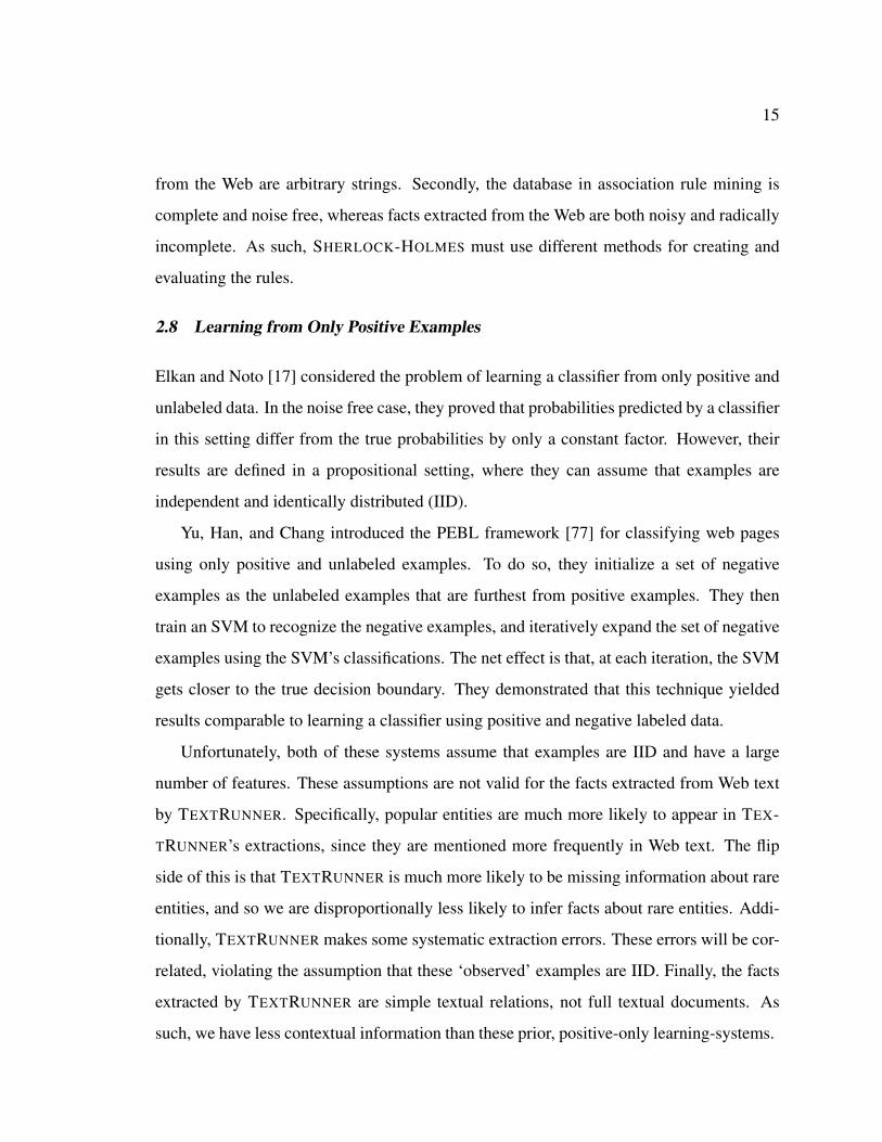
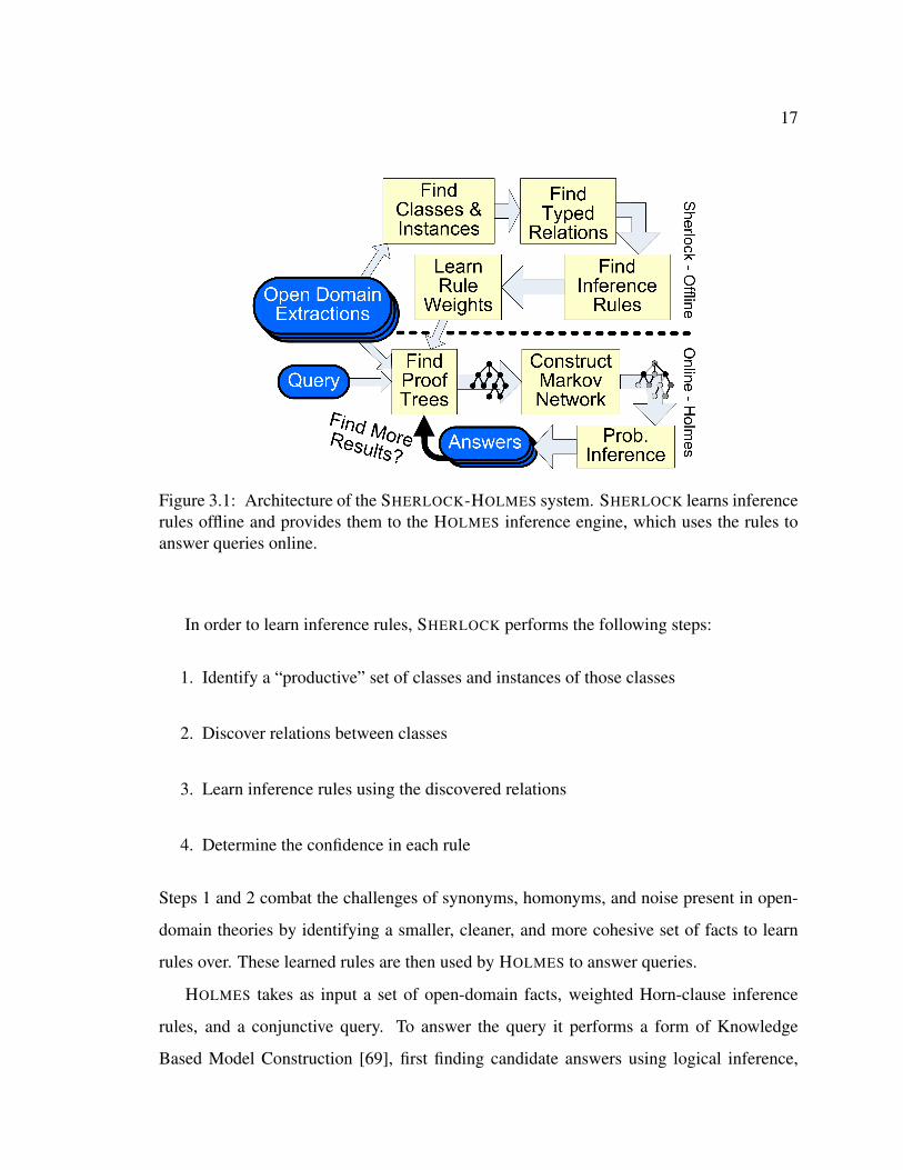
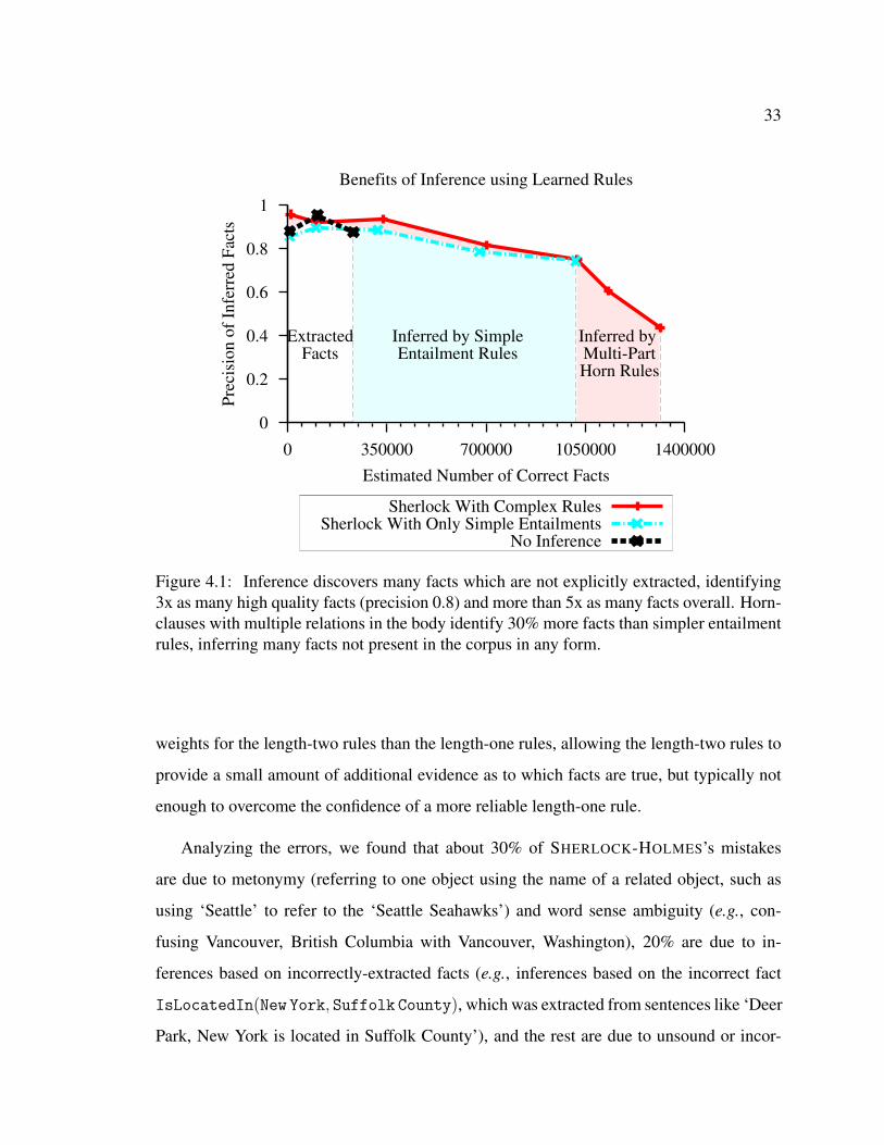
Figure 4.1 compares the precision and estimated number of correct facts with and with-
out inference. As is apparent, the learned rules substantially increase the number of correct
facts, quadrupling the relative recall beyond what is explicitly extracted. The length-two
Horn-rules boost relative recall by 30% over the simpler length-one rules. Furthermore, the
Horn-rules yield slightly increased precision at comparable levels of recall, although the
increase is not statistically significant. This behavior can be attributed to learning smaller
33
0
0.2
0.4
0.6
0.8
1
0 350000 700000 1050000 1400000
Pre
cisi
on
of
Infe
rred
Fac
ts
Estimated Number of Correct Facts
Benefits of Inference using Learned Rules
Sherlock With Complex RulesSherlock With Only Simple Entailments
No Inference
Inferred by SimpleEntailment Rules
Inferred by Multi-PartHorn Rules
ExtractedFacts
Figure 4.1: Inference discovers many facts which are not explicitly extracted, identifying3x as many high quality facts (precision 0.8) and more than 5x as many facts overall. Horn-clauses with multiple relations in the body identify 30% more facts than simpler entailmentrules, inferring many facts not present in the corpus in any form.
weights for the length-two rules than the length-one rules, allowing the length-two rules to
provide a small amount of additional evidence as to which facts are true, but typically not
enough to overcome the confidence of a more reliable length-one rule.
Analyzing the errors, we found that about 30% of SHERLOCK-HOLMES’s mistakes
are due to metonymy (referring to one object using the name of a related object, such as
using ‘Seattle’ to refer to the ‘Seattle Seahawks’) and word sense ambiguity (e.g., con-
fusing Vancouver, British Columbia with Vancouver, Washington), 20% are due to in-
ferences based on incorrectly-extracted facts (e.g., inferences based on the incorrect fact
IsLocatedIn(New York, Suffolk County), which was extracted from sentences like ‘Deer
Park, New York is located in Suffolk County’), and the rest are due to unsound or incor-
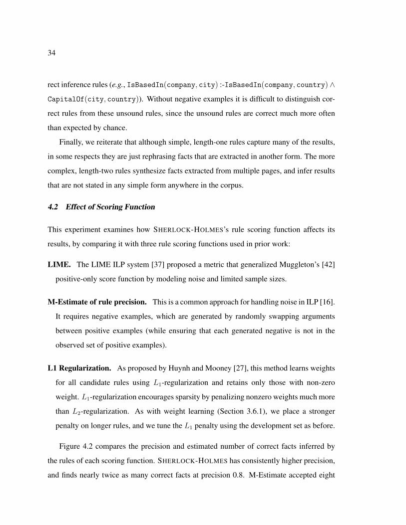
34
rect inference rules (e.g., IsBasedIn(company, city) :-IsBasedIn(company, country) ∧
CapitalOf(city, country)). Without negative examples it is difficult to distinguish cor-
rect rules from these unsound rules, since the unsound rules are correct much more often
than expected by chance.
Finally, we reiterate that although simple, length-one rules capture many of the results,
in some respects they are just rephrasing facts that are extracted in another form. The more
complex, length-two rules synthesize facts extracted from multiple pages, and infer results
that are not stated in any simple form anywhere in the corpus.
4.2 Effect of Scoring Function
This experiment examines how SHERLOCK-HOLMES’s rule scoring function affects its
results, by comparing it with three rule scoring functions used in prior work:
LIME. The LIME ILP system [37] proposed a metric that generalized Muggleton’s [42]
positive-only score function by modeling noise and limited sample sizes.
M-Estimate of rule precision. This is a common approach for handling noise in ILP [16].
It requires negative examples, which are generated by randomly swapping arguments
between positive examples (while ensuring that each generated negative is not in the
observed set of positive examples).
L1 Regularization. As proposed by Huynh and Mooney [27], this method learns weights
for all candidate rules using L1-regularization and retains only those with non-zero
weight. L1-regularization encourages sparsity by penalizing nonzero weights much more
than L2-regularization. As with weight learning (Section 3.6.1), we place a stronger
penalty on longer rules, and we tune the L1 penalty using the development set as before.
Figure 4.2 compares the precision and estimated number of correct facts inferred by
the rules of each scoring function. SHERLOCK-HOLMES has consistently higher precision,
and finds nearly twice as many correct facts at precision 0.8. M-Estimate accepted eight
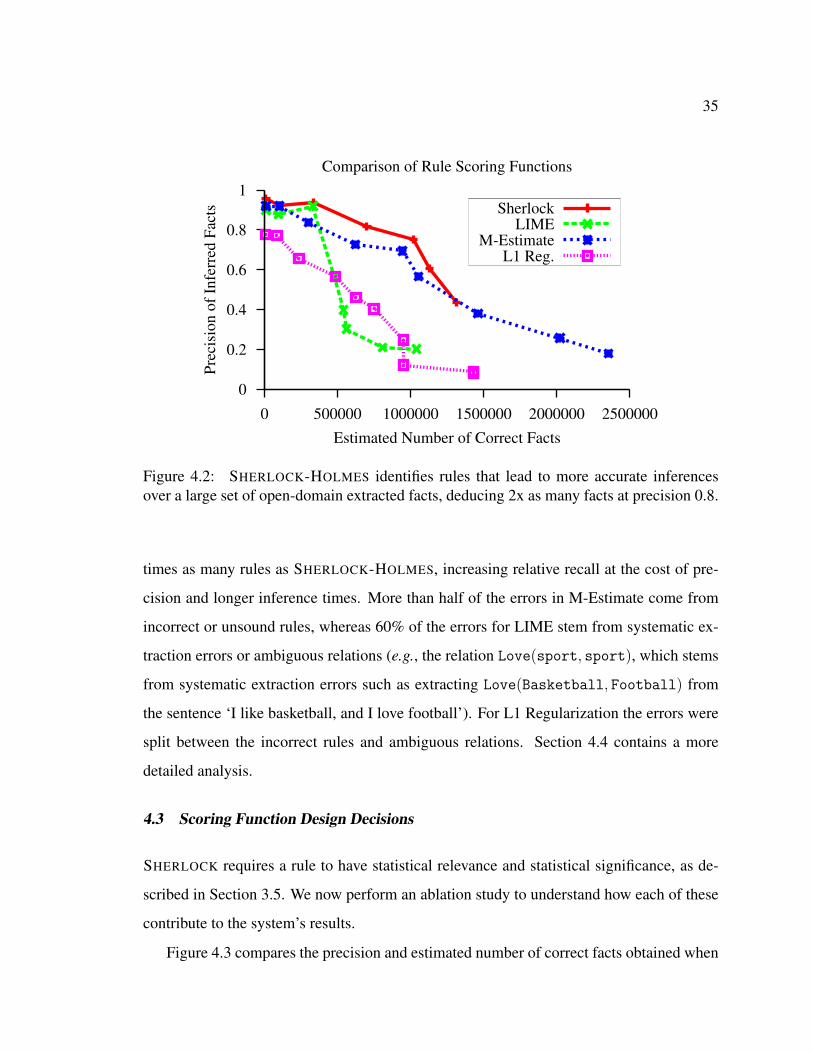
35
0
0.2
0.4
0.6
0.8
1
0 500000 1000000 1500000 2000000 2500000
Pre
cisi
on
of
Infe
rred
Fac
ts
Estimated Number of Correct Facts
Comparison of Rule Scoring Functions
SherlockLIME
M-EstimateL1 Reg.
Figure 4.2: SHERLOCK-HOLMES identifies rules that lead to more accurate inferencesover a large set of open-domain extracted facts, deducing 2x as many facts at precision 0.8.
times as many rules as SHERLOCK-HOLMES, increasing relative recall at the cost of pre-
cision and longer inference times. More than half of the errors in M-Estimate come from
incorrect or unsound rules, whereas 60% of the errors for LIME stem from systematic ex-
traction errors or ambiguous relations (e.g., the relation Love(sport, sport), which stems
from systematic extraction errors such as extracting Love(Basketball, Football) from
the sentence ‘I like basketball, and I love football’). For L1 Regularization the errors were
split between the incorrect rules and ambiguous relations. Section 4.4 contains a more
detailed analysis.
4.3 Scoring Function Design Decisions
SHERLOCK requires a rule to have statistical relevance and statistical significance, as de-
scribed in Section 3.5. We now perform an ablation study to understand how each of these
contribute to the system’s results.
Figure 4.3 compares the precision and estimated number of correct facts obtained when
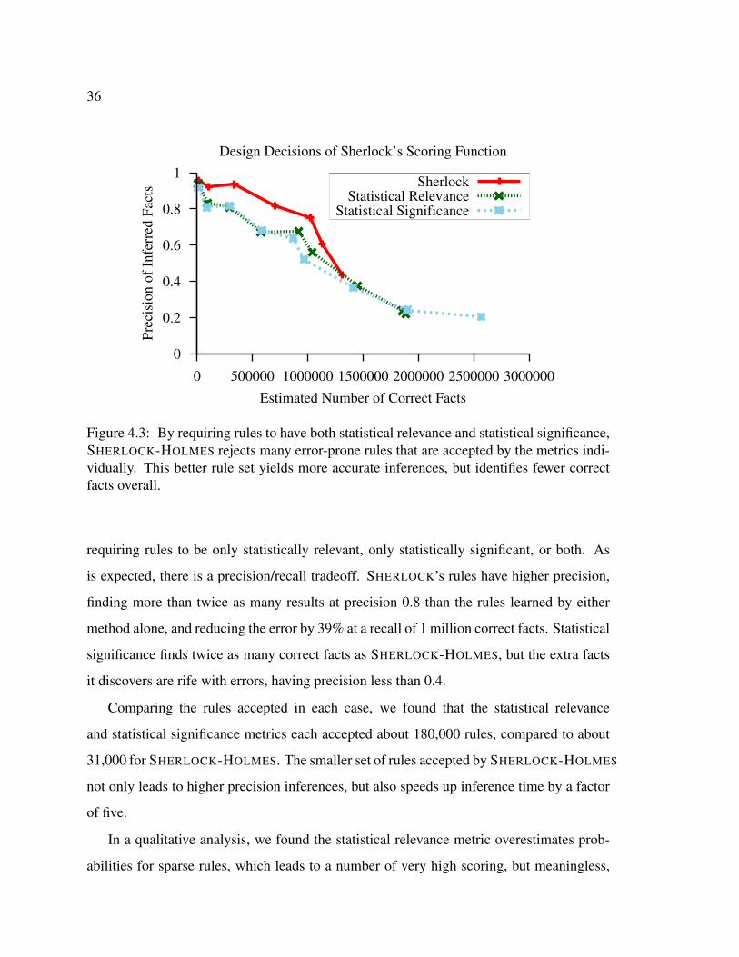
36
0
0.2
0.4
0.6
0.8
1
0 500000 1000000 1500000 2000000 2500000 3000000
Pre
cisi
on
of
Infe
rred
Fac
ts
Estimated Number of Correct Facts
Design Decisions of Sherlock’s Scoring Function
SherlockStatistical Relevance
Statistical Significance
Figure 4.3: By requiring rules to have both statistical relevance and statistical significance,SHERLOCK-HOLMES rejects many error-prone rules that are accepted by the metrics indi-vidually. This better rule set yields more accurate inferences, but identifies fewer correctfacts overall.
requiring rules to be only statistically relevant, only statistically significant, or both. As
is expected, there is a precision/recall tradeoff. SHERLOCK’s rules have higher precision,
finding more than twice as many results at precision 0.8 than the rules learned by either
method alone, and reducing the error by 39% at a recall of 1 million correct facts. Statistical
significance finds twice as many correct facts as SHERLOCK-HOLMES, but the extra facts
it discovers are rife with errors, having precision less than 0.4.
Comparing the rules accepted in each case, we found that the statistical relevance
and statistical significance metrics each accepted about 180,000 rules, compared to about
31,000 for SHERLOCK-HOLMES. The smaller set of rules accepted by SHERLOCK-HOLMES
not only leads to higher precision inferences, but also speeds up inference time by a factor
of five.
In a qualitative analysis, we found the statistical relevance metric overestimates prob-
abilities for sparse rules, which leads to a number of very high scoring, but meaningless,
37
rules. The statistical significance metric handles sparse rules better, but is still overconfident
in many unsound rules.
4.4 Analysis of Rule Scoring Functions
Pinpointing the exact cause of inference errors is difficult, especially when a fact is inferred
by multiple rules. Seemingly correct rules may have low precision if they incorporate
relations with many systematic extraction errors or ambiguous arguments. Should these
errors be attributed to the rule learner for accepting rules based on extraction errors, or to
the extractor for making the errors? To better understand the causes of errors we placed
each fact judged to be incorrect into one of three broad categories:
• Extraction Errors (Extr.) - The inference was based on an incorrectly extracted fact
or an ambiguous relation (e.g., Acquired(Google, Microsoft) or
Love(sport, sport) ). A perfect extractor would eliminate these errors.
• Unsound or Incorrect Inference Rule (Rule) - The inference was based on an rule
which is unsound or otherwise incorrect. To be placed in this category, the rule
used must consist of relations which are reasonable individually (not ambiguous or
systematic errors such as Love(sport, sport)), but are not combined in a sound way.
For example:
IsBasedIn(company, city):-IsBasedIn(company, place)∧IsLocatedIn(city, place);
• Metonymy and Word Sense Ambiguity (WSA) - The inference was based on an
incorrect interpretation of the arguments. For example, ambiguity about which city
Cambridge refers to may cause the system to infer that MIT is located in England.
Similarly, in the FIFA World Cup each nation’s team is metonymously referred to
by the country name (e.g., Beat(Germany, Uruguay)). Incorrect inferences based on
such ambiguities are placed into this category.
38
Although several of the judgements are subjective (e.g., how should one categorize a fact
inferred from both an unsound rule and a correct rule applied to an extraction error), the
general trends in the breakdown of errors should hold. Table 4.1 summarizes the number
of rules, inference time, relative recall at precision 0.8, total number of inferences, overall
precision, and a breakdown of the errors obtained when using each of the scoring functions.
The different rule scoring functions have different biases; Table 4.1 gives insight into
how each of their respective biases affect the results. For example, although the statistical
relevance and statistical significance metrics learn a similar number of rules, statistical rel-
evance takes less than half the time and infers a third fewer facts. This can be understood
from their respective biases. Statistical relevance prefers rules which behave like functions,
where each argument value appears in only a small number of the results. As such, statis-
tical relevance’s rules lead to fewer total inferences. The statistical significance metric, on
the other hand, prefers rules which predict more of the observed head values and rare head
values, but has a relatively small penalty for rules with a larger total number of inferences.
SHERLOCK’s rule scoring function requires both statistical relevance and statistical sig-
nificance, so it is unsurprising that it learns fewer rules and infers fewer facts overall. The
extra time needed to compute both statistical relevance and statistical significance is fairly
minor because they rely in the same set of probability estimates, and so eliminating more
rules allows SHERLOCK to run in less time over-all. What is surprising is that the relative
proportion of errors changes, making more errors due to word sense ambiguity than any
of the others. In SHERLOCK’s scoring function, statistical relevance eliminates many of
the overly general rules and statistical significance eliminates many of the rules with little
support. However, there are a small set of relations about sporting events and company
acquisitions where the rules have strong correlations, but suffer from metonymy and word
sense ambiguity. For example, if San Diego played Seattle (in baseball) and Seattle played
San Jose (in soccer), then San Diego isn’t likely to play San Jose. However, if the system
used another city with a baseball team instead of San Jose, then the inference would be
reasonable. Given the ambiguous nature of facts within our corpus, even a perfect ruler
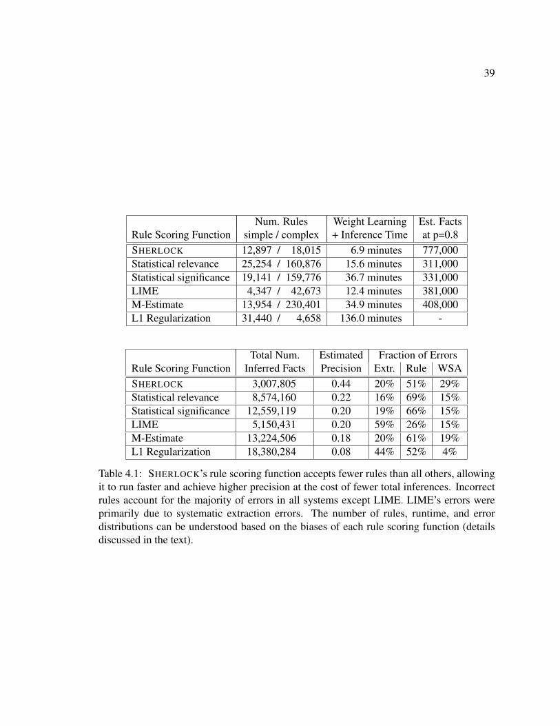
39
Num. Rules Weight Learning Est. FactsRule Scoring Function simple / complex + Inference Time at p=0.8SHERLOCK 12,897 / 18,015 6.9 minutes 777,000Statistical relevance 25,254 / 160,876 15.6 minutes 311,000Statistical significance 19,141 / 159,776 36.7 minutes 331,000LIME 4,347 / 42,673 12.4 minutes 381,000M-Estimate 13,954 / 230,401 34.9 minutes 408,000L1 Regularization 31,440 / 4,658 136.0 minutes -
Total Num. Estimated Fraction of ErrorsRule Scoring Function Inferred Facts Precision Extr. Rule WSASHERLOCK 3,007,805 0.44 20% 51% 29%Statistical relevance 8,574,160 0.22 16% 69% 15%Statistical significance 12,559,119 0.20 19% 66% 15%LIME 5,150,431 0.20 59% 26% 15%M-Estimate 13,224,506 0.18 20% 61% 19%L1 Regularization 18,380,284 0.08 44% 52% 4%
Table 4.1: SHERLOCK’s rule scoring function accepts fewer rules than all others, allowingit to run faster and achieve higher precision at the cost of fewer total inferences. Incorrectrules account for the majority of errors in all systems except LIME. LIME’s errors wereprimarily due to systematic extraction errors. The number of rules, runtime, and errordistributions can be understood based on the biases of each rule scoring function (detailsdiscussed in the text).
40
learner would make a number of mistakes due to word sense ambiguity. Although all of the
scoring functions accept rules which make such mistakes, SHERLOCK makes fewer total
mistakes due to incorrect rules or extraction errors. As such, the proportion of errors due to
word sense ambiguity is higher.
The M-Estimate rule scoring function favors rules with high precision on the labeled
data. It does not factor in the total number of facts the rule infers. However, rules which
infer more facts in total are likely to infer more correct facts coincidentally. Without a good
set of negative examples, these coincidental inferences will cause the M-Estimate scoring
function to rate such rules highly. Thus, as with the results for the statistical significance
metric, the rules M-Estimate learns tend to infer more facts overall.
The L1 Regularization rule scoring method is similar to M-Estimate in its biases, but
favors finding a small number of rules which ‘explain’ most of the observed facts. However,
because it places a larger L1-regularization penalty on longer rules, it accepts mainly short
rules. The small number of longer rules that it does accept tend to be rules which behave
like cross-products. For example, if there was a rule that inferred all |class1| × |class2|
values for a particular relation R(class1, class2), then that rule would ‘explain’ all of the
observed values despite the fact that the rule is most likely incorrect. As with M-Estimate,
this problem stems from not having a good set of negative examples. Additionally, it takes
significantly longer than all of the other systems. This is because it must perform weight
learning over all 4.9 million candidate rules that have sufficient support, whereas using the
other scoring functions only requires learning weights over high-scoring rules.
The LIME rule scoring function behaves differently than the other rule scoring func-
tions. The majority of its mistakes can be attributed to systematic extraction errors and the
rules that stem from them. For example, the LIME scoring function accepts many rules
using the relations Love(sport, sport) and Chop(food, food) (the latter of which stems
from systematic extraction errors such as extracting Chop(carrots, onions) from recipe
sentences like ‘Add peeled carrots, chopped onions, and diced celery to pot’). These rela-
tions have dense subsets, where many of the possible values of the relation occur together
41
(e.g., many recipes call for adding some chopped vegetable after some previous step). Al-
though LIME penalizes each rule based on the total number of facts it infers, it also assumes
that the observed facts and errors are drawn randomly. Relations based on systematic ex-
traction errors violate this assumption, causing rules inferring such relations to appear to
have substantial support.
Finally, although the final precision in all cases is fairly low, such low precision results
may be useful for applications preferring high recall. We compared the results to two types
of random guessing - uniform sampling and biased sampling. In the first case, we sampled
instances of the typed-relation R(class1, class2) uniformly and independently from all in-
stances of class{1,2}. However, since more companies are likely to be based in major cities,
famous people are more likely to attend major universities, etc., we also sampled instances
of each class{1,2} biased by how frequently the instance appeared with a Hearst pattern
for that class. We generated 250 random relation-instances according to each method and
evaluated them as before. The uniform random-sampling method had a precision less than
0.01. The biased random-sampling method did much better, having precision 0.09. All
scoring functions except L1 Regularization are at least twice as good as random guessing,
and SHERLOCK’s inference rules outperform random guessing by a factor of five.
4.5 Analysis of Weight Learning
Finally, we empirically validate the modifications of the weight learning algorithm from
Section 3.6.1.
The learned weights do not affect which facts are inferred, they only affect the confi-
dence of each inferred fact. For a fixed set of rules, the set of results inferred by the system
will remain the same. Thus, to measure the influence of the weight learning algorithm we
hold the rules constant and examine how the following modifications affect the probabilities
of the inferred facts:
• Fixed vs. Variable Penalty - Do we use the same L2 penalty on the weights for all
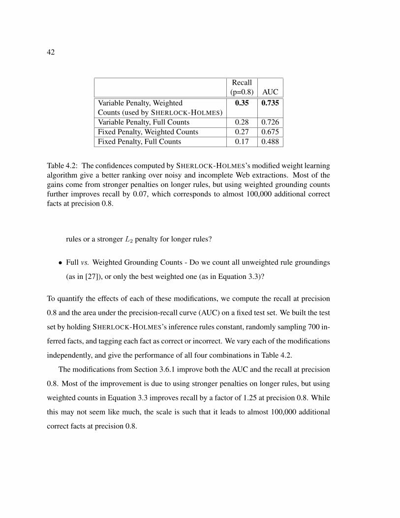
42
Recall(p=0.8) AUC
Variable Penalty, Weighted 0.35 0.735Counts (used by SHERLOCK-HOLMES)Variable Penalty, Full Counts 0.28 0.726Fixed Penalty, Weighted Counts 0.27 0.675Fixed Penalty, Full Counts 0.17 0.488
Table 4.2: The confidences computed by SHERLOCK-HOLMES’s modified weight learningalgorithm give a better ranking over noisy and incomplete Web extractions. Most of thegains come from stronger penalties on longer rules, but using weighted grounding countsfurther improves recall by 0.07, which corresponds to almost 100,000 additional correctfacts at precision 0.8.
rules or a stronger L2 penalty for longer rules?
• Full vs. Weighted Grounding Counts - Do we count all unweighted rule groundings
(as in [27]), or only the best weighted one (as in Equation 3.3)?
To quantify the effects of each of these modifications, we compute the recall at precision
0.8 and the area under the precision-recall curve (AUC) on a fixed test set. We built the test
set by holding SHERLOCK-HOLMES’s inference rules constant, randomly sampling 700 in-
ferred facts, and tagging each fact as correct or incorrect. We vary each of the modifications
independently, and give the performance of all four combinations in Table 4.2.
The modifications from Section 3.6.1 improve both the AUC and the recall at precision
0.8. Most of the improvement is due to using stronger penalties on longer rules, but using
weighted counts in Equation 3.3 improves recall by a factor of 1.25 at precision 0.8. While
this may not seem like much, the scale is such that it leads to almost 100,000 additional
correct facts at precision 0.8.
43
Chapter 5
SCALING SHERLOCK-HOLMES TO THE WEB
The previous chapters demonstrated the utility of SHERLOCK-HOLMES, showing that
it significantly increases recall over what is explicitly extracted. However, to operate at
Web scale inference also needs to be efficient.
In the general case, logical inference over a Horn theory is polynomial in the number of
ground facts, and hence in the size of the corpus.1 This is problematic, since even low-order
polynomial growth is prohibitive on the TEXTRUNNER [4] corpus, let alone the full Web.
Fortunately, the Web’s long tail works in our favor. The relations TEXTRUNNER extracts
from the Web are “approximately” functional in a well-defined sense. Formally, we say that
such relations are approximately pseudo-functional (APF), a property which guarantees that
SHERLOCK-HOLMES’s inference will scale linearly in the size of the corpus.
The following example illustrates the intuitions. Consider the rule
R(x, z) : −Married(x, y) ∧ LivedIn(y, z);
In the worst case, there is some person y who married everyone and who lived in every
place. This rule will then generate a polynomial (O(|Married| ∗ |LivedIn|)) number of
results. However, this worst-case scenario rarely occurs for relations mentioned on the
Web. The relations in this example are APF — most people have at most a few spouses,
and live in only a few places — so in general this rule will infer a much smaller number of
results from each person y than the worst case predicts. The definition of APF quantifies
‘most’ and ‘few’, and allows us to prove that SHERLOCK-HOLMES’s inference over APF
1In fact, it is P-complete – as hard as any polynomial-time problem
44
relations scales linearly in the size of the corpus.
This chapter examines how SHERLOCK-HOLMES scales with respect to both infer-
ence and rule learning. We formalize the approximately pseudo-functional property in
Section 5.1 and show how it ensures that HOLMES’s inference scales linearly. Section 5.2
then demonstrates empirically that most relations are APF, and that HOLMES’s inference
scales linearly in practice. We then extend the analysis to include rule-learning in SHER-
LOCK, showing that the system scales linearly in the size of the corpus (Section 5.3) and in
the number of relations considered (Section 5.4).
5.1 The Approximately Pseudo-Functional Property
HOLMES was designed to infer answers to queries using facts extracted from Web pages.
However, to be useful it must be able to infer these answers in a reasonable amount of time.
If it is applied to a corpus containing hundreds of millions or even billions of pages, its run
time has to be at most linear in the size of the corpus. This section shows that, under some
reasonable assumptions, inference does scale linearly.
In this section we assume that the query and set of inference rules given as input to
HOLMES is fixed. We analyze this case first, and remove this assumption in later sections.
Our analysis makes three additional assumptions.
Assumption 1. The number of distinct, ground facts in the KB, |F |, grows at most linearly
with the size of the corpus.
This assumption is certainly true for facts extracted by TEXTRUNNER and Kylin [70],
and follows from our exclusion of texts with complex quantified sentences. Our analysis
now proceeds to consider scaling with respect to |F | for a fixed query and set of inference
rules (i.e., “data complexity” in database lingo.)
Assumption 2. The body of each rule is a connected clause.
In general, we want the objects we are making inferences over to be related in some
way. Without this assumption, a rule may compute a cross-product combining all results
45
from one subclause with all results from another. Although this can occasionally be useful,
it rarely is for facts extracted from the Web. SHERLOCK and most other ILP systems only
consider connected rules, and in practice this limitation on expressivity allows us to avoid
computing cross-products, leading to a huge improvements in speed and memory usage.
Assumption 3. The size of every proof tree is bounded by some constant, m.
This is a strong assumption and one that depends on the precise set of inference rules
and pattern of ground facts. However, this limitation is useful in practice, since larger proof
trees are more likely to contain errors. It can be enforced by limiting the search for proof
trees to a certain depth, e.g., log(m), and by disallowing recursive rules or allowing only
a limited depth of recursion. These limitations are already required by the weight learning
and probabilistic inference method described in Section 3.6.
HOLMES’s inference has three steps:
1. Logical inference to construct a proof forest identifying the answers
2. Conversion of the forest into a Markov network
3. Probabilistic inference over that network.
The probabilistic inference method used by SHERLOCK-HOLMES runs in time linear in the
size of the Markov network. Since the Markov network is essentially isomorphic to the
proof forest, the conversion will take O(|F |) time and space if the forest is linear in size,
which is ensured if the time to construct the proof trees is O(|F |). We show this bounded
construction time is in fact the case in the remainder of this section.
HOLMES requires inference rules to be function-free, first-order Horn clauses. While
this limits expressivity to some degree, it provides a huge speed benefit; logical inference
over Horn clauses can be done in polynomial time, whereas general propositional inference
(i.e., from grounded first-order rules) is NP-complete.
46
Alas, even low-order polynomial blowup is unacceptable when the corpus reaches Web
scale; it must have linear growth. Intuitively, there are two places where polynomial ex-
pansion could cause trouble. First, the number of different types of proofs (i.e., first-order
proofs) could grow too quickly, and secondly, a given type of proof tree might apply to too
many ground facts (i.e., “tuples” in database terminology). We treat these issues in turn.
Under the above assumptions, each proof tree can be represented as an expression in
relational algebra with at most m equijoins [66],2 each stemming from the application of
an inference rule. Since the number of rules is fixed, as is m, there are a constant number
of possible first-order proof trees.
The bigger concern is that any one of these first-order trees might result in a polynomial
number of ground trees; if so, the size of the ground forest (and corresponding Markov
network) could grow too quickly. In fact, polynomial growth is a common phenomena
in database query evaluation. Fortunately, most relations in the Web corpus behave more
favorably. We introduce a property of relations that ensuresm-way equijoins, and therefore
all proof trees up to size m, can be computed in O(|F |) time.
The intuition for this property is that most relations derived from large corpora have a
‘long-tailed’ distribution, wherein a few objects appear many times in a relation, but most
appear only once or twice. Therefore, joins involving rare objects lead to a small number
of results, and so the main limitation on scalability is common objects. We now prove that
if these common objects account for a small enough fraction of the relation, then joins will
still scale linearly. We focus on binary relations, but these results can easily be extended to
relations of larger arity.
Definition 3. A relation, R = {(xi, yi)} ⊆ X × Y , is pseudo-functional (PF) in x with
degree k, if ∀x ∈ X : |{y|(x, y) ∈ R}| ≤ k. When the precise variable and degree is
irrelevant to the discussion, we simply say “R is PF.”
2Note that an inference rule of the form H(X) : −R1(X, Y) ∧ R2(Y, Z) is equivalent to the algebraic expres-sion πX(R1 ./ R2). First a join is performed between R1 and R2 testing for equality between values ofY ; then a projection eliminates all columns besides X .
47
An m-way equijoin over relations that are PF in the join variables will have at most
km ∗ |R| results. Since km is constant for a given join and |R| scales linearly in the size of
the textual corpus, proof tree construction over PF relations also scales linearly.
However, due to their long-tailed distributions, most relations extracted from the Web
fit the pseudo-functional definition in most, but not all values of X . Fortunately, in most
cases these “bad” values of X are rare and hence do not influence the join size significantly.
We formalize this intuition by defining a class of approximately pseudo-functional (APF)
relations and proving that joining two APF relations produces at most a linear number of
results.
Definition 4. A relation, R = {(xi, yi)} ⊆ X × Y , is approximately pseudo-functional
(APF) in x with degree k, if X can be partitioned into two sets XG and XB such that for all
x ∈ XG R is PF with degree k and x ∈ XB have∑
x∈XB
|{y|(x, y) ∈ R}| ≤ k ∗ log(|R|)
Theorem 1. If relation R1 is APF in y with degree k1 and R2 is APF in y with degree k2
then the relation Q = R1 ./ R2 has size at most O(max(|R1|, |R2|)).
Proof. Since R1 and R2 are APF, we know that Y can be partitioned into four groups:
YBB = YB1⋂YB2, YBG = YB1
⋂YG2, YGB = YG1
⋂YB2, YGG = YG1
⋂YG2.3 We can
show that each group leads to at most O(|F |) entries in Q. For y ∈ YBB there are at most
k1 ∗ k2 ∗ log(|R1|) ∗ log(|R2|) entries in Q. The y ∈ YGB and y ∈ YBG lead to at most
k1 ∗ k2 ∗ log(|R2|) and k1 ∗ k2 ∗ log(|R1|) entries, respectively. For y ∈ YGG there are at
most k1 ∗ k2 ∗max(|R1|, |R2|). Summing the results from the four partitions, we see that
|Q| is O(max(|R1|, |R2|)), thus it is O(|F |).
This theorem and proof can easily be extended to an m-way equijoin, as long as each
relation is APF in all arguments that are being joined.
3YBB are the “doubly bad” values of y that violate the PF definition for both relations, YGG are the valuesthat do not violate the PF definition for either relation, and YBG and YGB are the values that violate it inonly R1 or R2, resp.

48
Theorem 2. IfQ is the relation obtained by an equijoin over m relationsR1..m, each having
size at most O(|F |), and if all R1..m are APF in all arguments that they are joined in with
degree at most kmax, and if∏
1≤i≤m
log(|Ri|) ≤ c ∗ |F | for some constant c, then |Q| is
O(|F |).
The proof of this is a straightforward extension of the proof of Theorem 1.
Proof Sketch. We partition the domain of each Ri and each argument into sets of ‘good’
and ‘bad’ values (which meet or violate, respectively, the pseudo-functional definition).
Each result of the join must come from exactly one combination of those sets, so we can
partition Q into a fixed number of sets accordingly. Performing a case-by-case analysis as
before, we can show that each partition yields at most O(|F |) results. Therefore, the sum
over the fixed set of partitions must be O(|F |), and so |Q| must also be at most O(|F |).
The inequality in Theorem 2 relates the sizes of the relations (|R|), the size of the
equijoin (m), and the number of ground facts (|F |). In particular, given Assumption 1 this
inequality is guaranteed to hold if the join size m is O(log|F |/log log|F |). However, in
many cases we are interested in much smaller joins than the inequality allows. For example,
the rules learned by SHERLOCK in Chapter 4 as well as the manually crafted rules in [57]
lead to proof-trees having at most m = 2-way equijoins. If we are willing to limit the
maximum join size, we can relax the APF definition to allow a broader, but still scalable,
class of m-way-APF relations.
Corollary 3. If Q is the relation obtained by an m-way join, and if each participating
relation is APF in their joined variables with a bound of ki∗ m√|Ri| instead of ki∗log(|Ri|),
then the join is O(|F |).
The proof of this is similar to the proof of Theorem 2. Using ki ∗ m√|Ri| in the case-
by-case analysis also allows us to show that each group is O(|F |). For example, in the
49
2-way-join case, the “doubly bad” term y ∈ YBB would be k1 ∗ k2 ∗√|R1| ∗
√|R2| ≤
const ∗√|F | ∗
√|F | = O(|F |). Since each partition is O(|F |), their sum is also O(|F |).
The final step in our scaling argument concerns probabilistic inference, which is #P-
Complete if performed exactly. This can be addressed in two ways. First, when using a
closed-form, discriminative inference method (Section 3.6), the probabilities can be com-
puted exactly in time linear in the size of the proof forest. Second, when not using that
method, HOLMES may alternatively use approximate methods (e.g., loopy belief propa-
gation) which avoid the cost of exact inference — at the cost of reduced accuracy. Fur-
thermore, at a practical level, HOLMES’s incremental construction of the Markov network
allows it to artificially bound the size of the network and the cost of inference by terminating
the search for additional proofs.
5.2 Scalability of Inference
As shown in the previous section, for approximately pseudo-functional relations HOLMES’s
inference will scale linearly in the size of the corpus. This section addresses two empirical
questions from those results. First, how common are APF relations in facts extracted from
the Web? Second, how does HOLMES’s runtime scale in practice?
To determine the prevalence of APF relations in Web text, we examined a sample of
500 binary relations selected randomly from TEXTRUNNER’s ground facts. The surface
forms of the relations and arguments may misrepresent the true properties of the under-
lying concepts. To better estimate the true properties we ignored type information in this
experiment, and instead merged synonymous values as given by Resolver [74] or the most
frequent sense of the word in WordNet [39]. For example, in this experiment we con-
sider BornIn(baby, hospital) and BornAt(infant, infirmary) to represent the same
concept, and merged them into one instance of the ‘Born In’ relation. The largest two rela-
tions had over 1.25 million unique instances each, and 52% of the relations had more than
10,000 instances.
For each relation R, we first found all instances of R extracted by TEXTRUNNER and
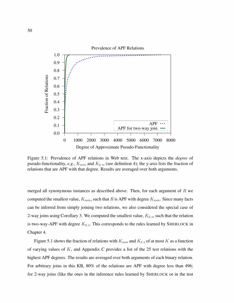
50
0.0
0.1
0.2
0.3
0.4
0.5
0.6
0.7
0.8
0.9
1.0
0 1000 2000 3000 4000 5000 6000 7000 8000
Fra
ctio
n o
f R
elat
ions
Degree of Approximate Pseudo-Functionality
Prevalence of APF Relations
APFAPF for two-way join
Figure 5.1: Prevalence of APF relations in Web text. The x-axis depicts the degree ofpseudo-functionality, e.g., Kmin and K2./, (see definition 4); the y-axis lists the fraction ofrelations that are APF with that degree. Results are averaged over both arguments.
merged all synonymous instances as described above. Then, for each argument of R we
computed the smallest value,Kmin, such thatR is APF with degreeKmin. Since many facts
can be inferred from simply joining two relations, we also considered the special case of
2-way joins using Corollary 3. We computed the smallest value, K2./, such that the relation
is two-way-APF with degree K2./. This corresponds to the rules learned by SHERLOCK in
Chapter 4.
Figure 5.1 shows the fraction of relations withKmin andK2./ of at mostK as a function
of varying values of K, and Appendix C provides a list of the 25 test relations with the
highest APF degrees. The results are averaged over both arguments of each binary relation.
For arbitrary joins in this KB, 80% of the relations are APF with degree less than 496;
for 2-way joins (like the ones in the inference rules learned by SHERLOCK or in the test
51
questions in Schoenmackers et al. [57] ), 80% of the relations are APF with degree less
than 65. These results indicate that the majority of relations TEXTRUNNER extracted from
text are APF, and so we can expect HOLMES’s techniques will allow efficient inference
over most relations.
The sharp rise for low values of K in the graphs is ideal, since it indicates that the vast
majority of relations are APF with a fairly small degree. Since the APF degree (K) acts
as a constant scaling factor in HOLMES’s inference, smaller values of K lead to smaller
probabilistic networks, and allow HOLMES to operate faster or handle larger relations with
less space. Thus, Figure 5.1 indicates that even in limited environments HOLMES can
perform inference over a large number of relations.
However, although Theorem 2 guarantees that joins over such relations will be O(|F |),
that notation hides a potentially large constant factor of Kminm. This can potentially make
inference expensive, even for relatively small values of K. Fortunately, the constant factor
is significantly smaller in practice. To see why, we re-examine the proof: the large factor
comes from assuming that all of the relation’s first arguments that meet the PF definition
are associated with exactly Kmin distinct second arguments. However, in our corpus 83%
of first arguments are associated with only one second argument. Clearly, our worst-case
analysis substantially over-estimates inference time for most queries. Moreover, the mea-
sured join sizes and number of inferred results grew linearly in the size of the corpus, but
were on average two to three orders of magnitude smaller than the bounds given in the
theory. This observation held across relations with different sizes and values of Kmin.
While the results in Figure 5.1 may vary for other extraction systems or sets of rela-
tions, we believe the general trend holds. This is promising for HOLMES, as well as for
other Question Answering and Textual Inference systems. If true it implies that combining
information from multiple different sources is feasible, and can allow such systems to infer
answers not explicitly seen in any source.
Since most relations are APF in their arguments, our theory predicts HOLMES’s infer-
ence will scale linearly in the size of the corpus. We validate this empirically by measuring
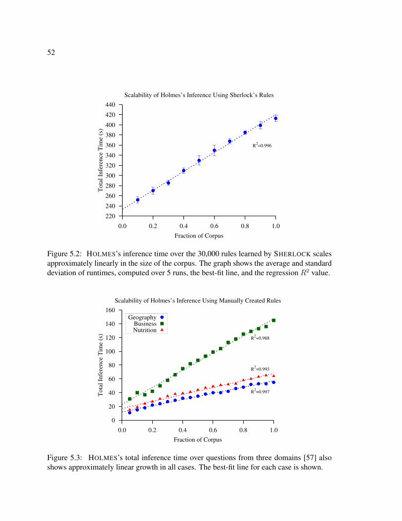
52
220
240
260
280
300
320
340
360
380
400
420
440
0.0 0.2 0.4 0.6 0.8 1.0
Tota
l In
fere
nce
Tim
e (s
)
Fraction of Corpus
Scalability of Holmes’s Inference Using Sherlock’s Rules
R2=0.996
Figure 5.2: HOLMES’s inference time over the 30,000 rules learned by SHERLOCK scalesapproximately linearly in the size of the corpus. The graph shows the average and standarddeviation of runtimes, computed over 5 runs, the best-fit line, and the regression R2 value.
0
20
40
60
80
100
120
140
160
0.0 0.2 0.4 0.6 0.8 1.0
Tota
l In
fere
nce
Tim
e (s
)
Fraction of Corpus
Scalability of Holmes’s Inference Using Manually Created Rules
R2=0.988
R2=0.993
R2=0.997
GeographyBusinessNutrition
Figure 5.3: HOLMES’s total inference time over questions from three domains [57] alsoshows approximately linear growth in all cases. The best-fit line for each case is shown.
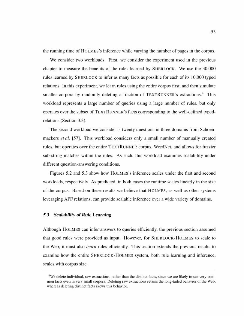
53
the running time of HOLMES’s inference while varying the number of pages in the corpus.
We consider two workloads. First, we consider the experiment used in the previous
chapter to measure the benefits of the rules learned by SHERLOCK. We use the 30,000
rules learned by SHERLOCK to infer as many facts as possible for each of its 10,000 typed
relations. In this experiment, we learn rules using the entire corpus first, and then simulate
smaller corpora by randomly deleting a fraction of TEXTRUNNER’s extractions.4 This
workload represents a large number of queries using a large number of rules, but only
operates over the subset of TEXTRUNNER’s facts corresponding to the well-defined typed-
relations (Section 3.3).
The second workload we consider is twenty questions in three domains from Schoen-
mackers et al. [57]. This workload considers only a small number of manually created
rules, but operates over the entire TEXTRUNNER corpus, WordNet, and allows for fuzzier
sub-string matches within the rules. As such, this workload examines scalability under
different question-answering conditions.
Figures 5.2 and 5.3 show how HOLMES’s inference scales under the first and second
workloads, respectively. As predicted, in both cases the runtime scales linearly in the size
of the corpus. Based on these results we believe that HOLMES, as well as other systems
leveraging APF relations, can provide scalable inference over a wide variety of domains.
5.3 Scalability of Rule Learning
Although HOLMES can infer answers to queries efficiently, the previous section assumed
that good rules were provided as input. However, for SHERLOCK-HOLMES to scale to
the Web, it must also learn rules efficiently. This section extends the previous results to
examine how the entire SHERLOCK-HOLMES system, both rule learning and inference,
scales with corpus size.
4We delete individual, raw extractions, rather than the distinct facts, since we are likely to see very com-mon facts even in very small corpora. Deleting raw extractions retains the long-tailed behavior of the Web,whereas deleting distinct facts skews this behavior.
54
The primary problem with applying the previous analysis is that the number of rules is
no longer constant. With a larger corpus, SHERLOCK has more evidence and will evaluate
and learn more rules. Indeed, Figure 5.4 shows that the number of rules SHERLOCK evalu-
ates (i.e., those that have sufficient support) and learns (i.e., those that have high statistical
relevance and statistical significance) both scale linearly in the size of the corpus. Since
each rule is O(|F |), if the number of rules increases then the total runtime may increase
super-linearly.
Fortunately, the rules learned by the system also have long-tailed behavior. Most typed-
relations have only a few rules inferring them, and only a small number of relations are
the head of a large number of rules. Figure 5.5 ranks the relations by the number of rules
inferring them, and shows that for 90% of the relations there are fewer than 8 rules inferring
the relation. This long-tailed behavior can be exploited by considering a second-order form
of approximate pseudo-functionality.
Our analysis requires the same assumptions as before, except rather than assuming that
the rules are given as input, we instead assume the following:
Assumption 4. The set of classes, instances, and typed relations is fixed as input to SHER-
LOCK’s rule learning component. Additionally, all of the typed relations are APF with
some degree K.
This assumption will be relaxed in the next section, but having a pre-defined notion of
the objects and relations of interest is a reasonable assumption in practice. Most ILP sys-
tems assume that objects and relations are given as input. Finally, most relations extracted
from the Web are APF, so assuming that all relations we use are APF is not a limitation in
practice.
Under the bounded proof-tree size assumption (Assumption 3), there are a fixed number
of templates describing the high-level structure of the proof tree. For example, SHERLOCK
learns rules of the form R1(x, y) : −R2(x, y), R1(x, z) : −R2(x, y) ∧ R3(y, z),
R1(x, z) : −R2(x, y) ∧ R3(z, y), etc. Such templates have been used in other rule learning
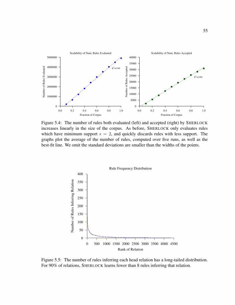
55
0
1000000
2000000
3000000
4000000
5000000
0.0 0.2 0.4 0.6 0.8 1.0
Num
ber
of
Rule
s E
val
uat
ed
Fraction of Corpus
Scalability of Num. Rules Evaluated
R2=0.998
0
5000
10000
15000
20000
25000
30000
35000
40000
0.0 0.2 0.4 0.6 0.8 1.0
Num
ber
of
Rule
s A
ccep
ted
Fraction of Corpus
Scalability of Num. Rules Accepted
R2=0.998
Figure 5.4: The number of rules both evaluated (left) and accepted (right) by SHERLOCK
increases linearly in the size of the corpus. As before, SHERLOCK only evaluates ruleswhich have minimum support s = 2, and quickly discards rules with less support. Thegraphs plot the average of the number of rules, computed over five runs, as well as thebest-fit line. We omit the standard deviations are smaller than the widths of the points.
0
50
100
150
200
250
300
350
400
0 500 1000 1500 2000 2500 3000 3500 4000 4500
Num
ber
of
Rule
s In
ferr
ing R
elat
ion
Rank of Relation
Rule Frequency Distribution
Figure 5.5: The number of rules inferring each head relation has a long-tailed distribution.For 90% of relations, SHERLOCK learns fewer than 8 rules inferring that relation.
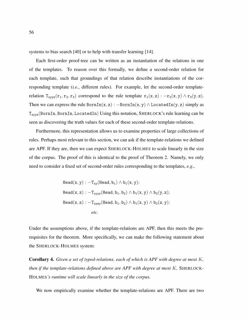
56
systems to bias search [40] or to help with transfer learning [14].
Each first-order proof-tree can be written as an instantiation of the relations in one
of the templates. To reason over this formally, we define a second-order relation for
each template, such that groundings of that relation describe instantiations of the cor-
responding template (i.e., different rules). For example, let the second-order template-
relation Txyyz(r1, r2, r3) correspond to the rule template r1(x, z) : −r2(x, y) ∧ r3(y, z).
Then we can express the rule BornIn(x, z) : −BornIn(x, y) ∧ LocatedIn(y, z) simply as
Txyyz(BornIn, BornIn, LocatedIn) Using this notation, SHERLOCK’s rule learning can be
seen as discovering the truth values for each of these second-order template-relations.
Furthermore, this representation allows us to examine properties of large collections of
rules. Perhaps most relevant to this section, we can ask if the template-relations we defined
are APF. If they are, then we can expect SHERLOCK-HOLMES to scale linearly in the size
of the corpus. The proof of this is identical to the proof of Theorem 2. Namely, we only
need to consider a fixed set of second-order rules corresponding to the templates, e.g.,
Head(x, y) : −Txy(Head, b1) ∧ b1(x, y);
Head(x, z) : −Txyyz(Head, b1, b2) ∧ b1(x, y) ∧ b2(y, z);
Head(x, z) : −Txyzy(Head, b1, b2) ∧ b1(x, y) ∧ b2(z, y);
etc.
Under the assumptions above, if the template-relations are APF, then this meets the pre-
requisites for the theorem. More specifically, we can make the following statement about
the SHERLOCK-HOLMES system:
Corollary 4. Given a set of typed-relations, each of which is APF with degree at most K,
then if the template-relations defined above are APF with degree at most K, SHERLOCK-
HOLMES’s runtime will scale linearly in the size of the corpus.
We now empirically examine whether the template-relations are APF. There are two
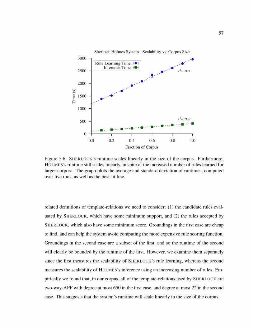
57
0
500
1000
1500
2000
2500
3000
0.0 0.2 0.4 0.6 0.8 1.0
Tim
e (s
)
Fraction of Corpus
Sherlock-Holmes System - Scalability vs. Corpus Size
R2=0.997
R2=0.996
Rule Learning TimeInference Time
Figure 5.6: SHERLOCK’s runtime scales linearly in the size of the corpus. Furthermore,HOLMES’s runtime still scales linearly, in spite of the increased number of rules learned forlarger corpora. The graph plots the average and standard deviation of runtimes, computedover five runs, as well as the best-fit line.
related definitions of template-relations we need to consider: (1) the candidate rules eval-
uated by SHERLOCK, which have some minimum support, and (2) the rules accepted by
SHERLOCK, which also have some minimum score. Groundings in the first case are cheap
to find, and can help the system avoid computing the more expensive rule scoring function.
Groundings in the second case are a subset of the first, and so the runtime of the second
will clearly be bounded by the runtime of the first. However, we examine them separately
since the first measures the scalability of SHERLOCK’s rule learning, whereas the second
measures the scalability of HOLMES’s inference using an increasing number of rules. Em-
pirically we found that, in our corpus, all of the template-relations used by SHERLOCK are
two-way-APF with degree at most 650 in the first case, and degree at most 22 in the second
case. This suggests that the system’s runtime will scale linearly in the size of the corpus.
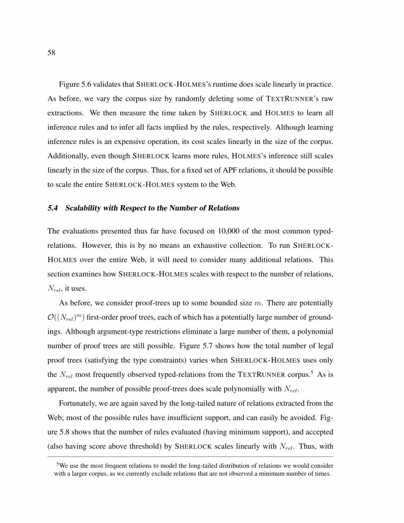
58
Figure 5.6 validates that SHERLOCK-HOLMES’s runtime does scale linearly in practice.
As before, we vary the corpus size by randomly deleting some of TEXTRUNNER’s raw
extractions. We then measure the time taken by SHERLOCK and HOLMES to learn all
inference rules and to infer all facts implied by the rules, respectively. Although learning
inference rules is an expensive operation, its cost scales linearly in the size of the corpus.
Additionally, even though SHERLOCK learns more rules, HOLMES’s inference still scales
linearly in the size of the corpus. Thus, for a fixed set of APF relations, it should be possible
to scale the entire SHERLOCK-HOLMES system to the Web.
5.4 Scalability with Respect to the Number of Relations
The evaluations presented thus far have focused on 10,000 of the most common typed-
relations. However, this is by no means an exhaustive collection. To run SHERLOCK-
HOLMES over the entire Web, it will need to consider many additional relations. This
section examines how SHERLOCK-HOLMES scales with respect to the number of relations,
Nrel, it uses.
As before, we consider proof-trees up to some bounded size m. There are potentially
O((Nrel)m) first-order proof trees, each of which has a potentially large number of ground-
ings. Although argument-type restrictions eliminate a large number of them, a polynomial
number of proof trees are still possible. Figure 5.7 shows how the total number of legal
proof trees (satisfying the type constraints) varies when SHERLOCK-HOLMES uses only
the Nrel most frequently observed typed-relations from the TEXTRUNNER corpus.5 As is
apparent, the number of possible proof-trees does scale polynomially with Nrel.
Fortunately, we are again saved by the long-tailed nature of relations extracted from the
Web; most of the possible rules have insufficient support, and can easily be avoided. Fig-
ure 5.8 shows that the number of rules evaluated (having minimum support), and accepted
(also having score above threshold) by SHERLOCK scales linearly with Nrel. Thus, with
5We use the most frequent relations to model the long-tailed distribution of relations we would considerwith a larger corpus, as we currently exclude relations that are not observed a minimum number of times.
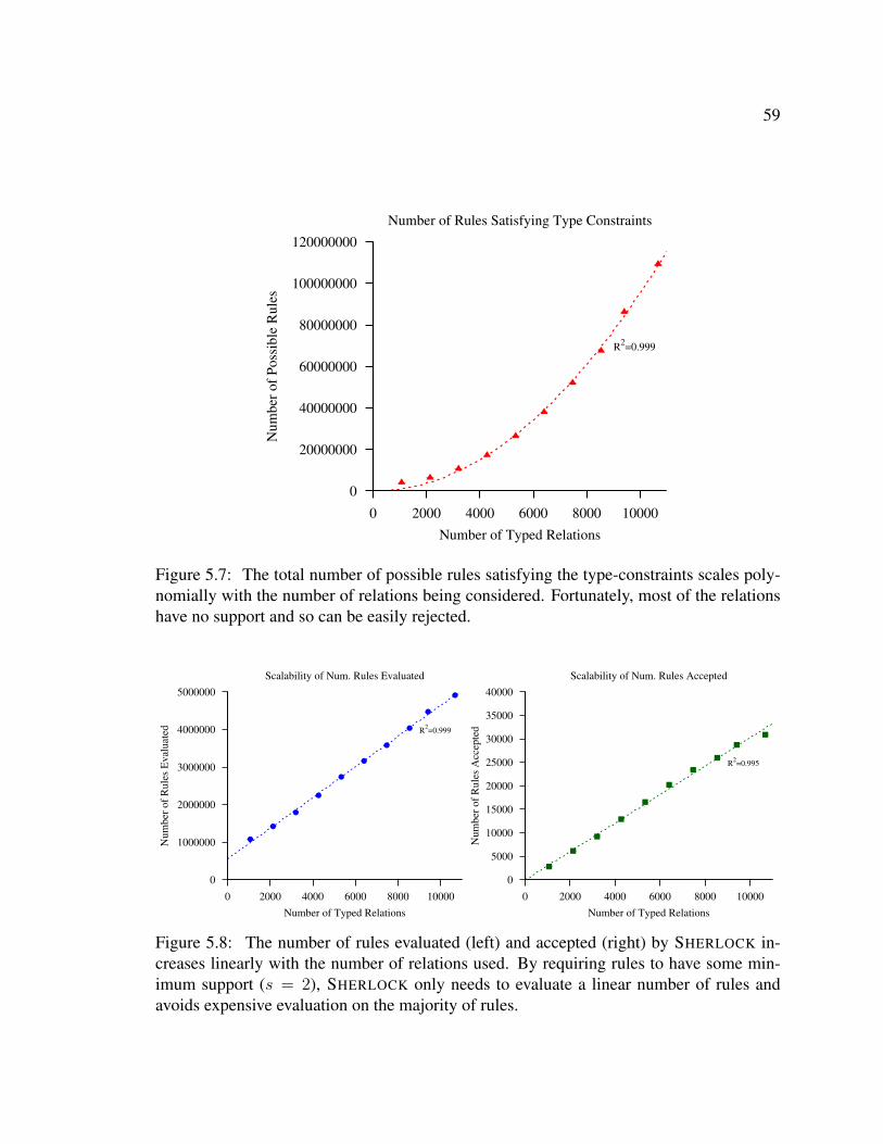
59
0
20000000
40000000
60000000
80000000
100000000
120000000
0 2000 4000 6000 8000 10000
Num
ber
of
Poss
ible
Rule
s
Number of Typed Relations
Number of Rules Satisfying Type Constraints
R2=0.999
Figure 5.7: The total number of possible rules satisfying the type-constraints scales poly-nomially with the number of relations being considered. Fortunately, most of the relationshave no support and so can be easily rejected.
0
1000000
2000000
3000000
4000000
5000000
0 2000 4000 6000 8000 10000
Num
ber
of
Rule
s E
val
uat
ed
Number of Typed Relations
Scalability of Num. Rules Evaluated
R2=0.999
0
5000
10000
15000
20000
25000
30000
35000
40000
0 2000 4000 6000 8000 10000
Num
ber
of
Rule
s A
ccep
ted
Number of Typed Relations
Scalability of Num. Rules Accepted
R2=0.995
Figure 5.8: The number of rules evaluated (left) and accepted (right) by SHERLOCK in-creases linearly with the number of relations used. By requiring rules to have some min-imum support (s = 2), SHERLOCK only needs to evaluate a linear number of rules andavoids expensive evaluation on the majority of rules.
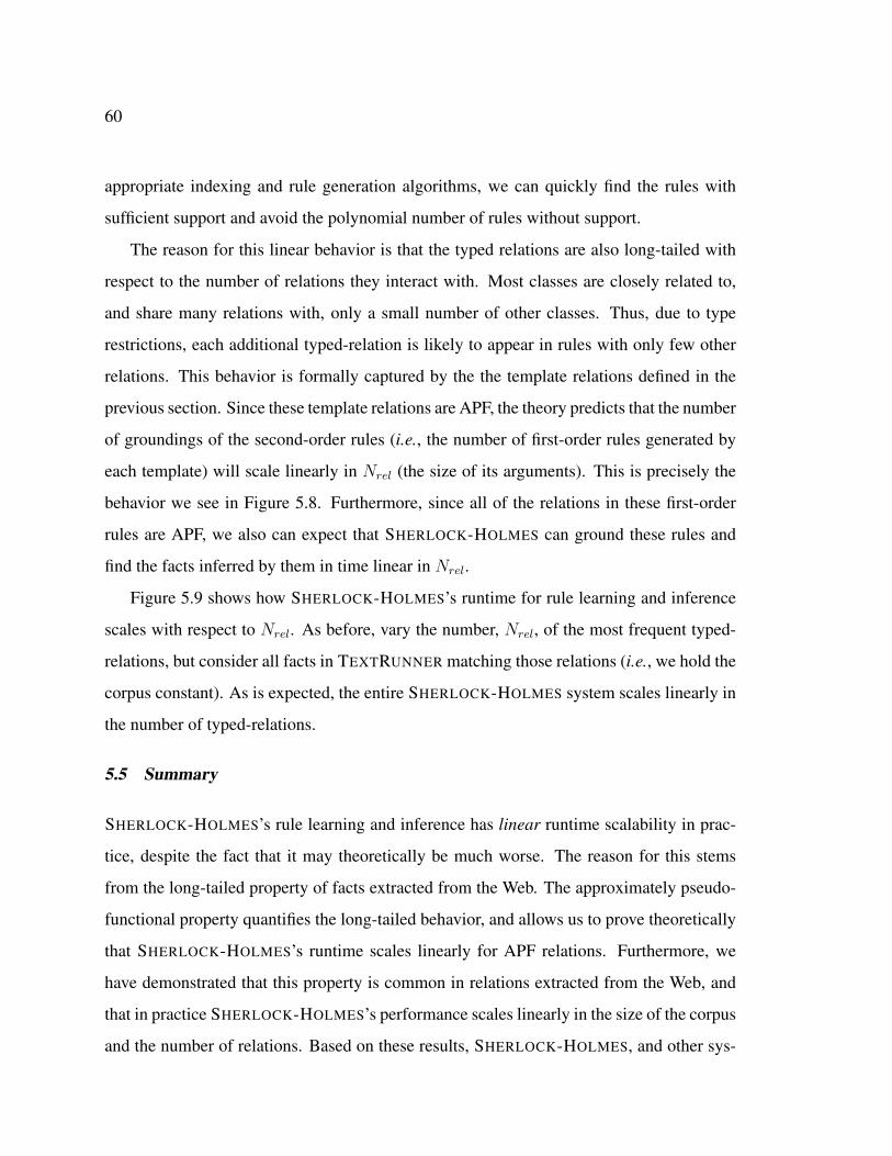
60
appropriate indexing and rule generation algorithms, we can quickly find the rules with
sufficient support and avoid the polynomial number of rules without support.
The reason for this linear behavior is that the typed relations are also long-tailed with
respect to the number of relations they interact with. Most classes are closely related to,
and share many relations with, only a small number of other classes. Thus, due to type
restrictions, each additional typed-relation is likely to appear in rules with only few other
relations. This behavior is formally captured by the the template relations defined in the
previous section. Since these template relations are APF, the theory predicts that the number
of groundings of the second-order rules (i.e., the number of first-order rules generated by
each template) will scale linearly in Nrel (the size of its arguments). This is precisely the
behavior we see in Figure 5.8. Furthermore, since all of the relations in these first-order
rules are APF, we also can expect that SHERLOCK-HOLMES can ground these rules and
find the facts inferred by them in time linear in Nrel.
Figure 5.9 shows how SHERLOCK-HOLMES’s runtime for rule learning and inference
scales with respect to Nrel. As before, vary the number, Nrel, of the most frequent typed-
relations, but consider all facts in TEXTRUNNER matching those relations (i.e., we hold the
corpus constant). As is expected, the entire SHERLOCK-HOLMES system scales linearly in
the number of typed-relations.
5.5 Summary
SHERLOCK-HOLMES’s rule learning and inference has linear runtime scalability in prac-
tice, despite the fact that it may theoretically be much worse. The reason for this stems
from the long-tailed property of facts extracted from the Web. The approximately pseudo-
functional property quantifies the long-tailed behavior, and allows us to prove theoretically
that SHERLOCK-HOLMES’s runtime scales linearly for APF relations. Furthermore, we
have demonstrated that this property is common in relations extracted from the Web, and
that in practice SHERLOCK-HOLMES’s performance scales linearly in the size of the corpus
and the number of relations. Based on these results, SHERLOCK-HOLMES, and other sys-
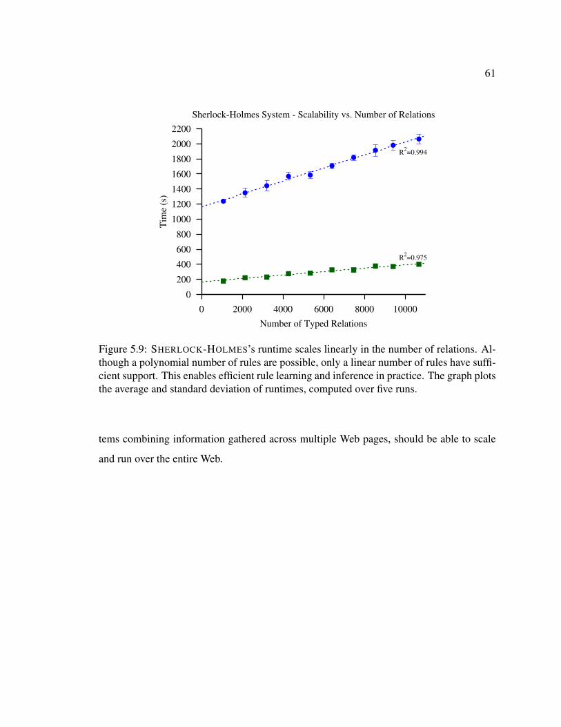
61
0
200
400
600
800
1000
1200
1400
1600
1800
2000
2200
0 2000 4000 6000 8000 10000
Tim
e (s
)
Number of Typed Relations
Sherlock-Holmes System - Scalability vs. Number of Relations
R2=0.994
R2=0.975
Figure 5.9: SHERLOCK-HOLMES’s runtime scales linearly in the number of relations. Al-though a polynomial number of rules are possible, only a linear number of rules have suffi-cient support. This enables efficient rule learning and inference in practice. The graph plotsthe average and standard deviation of runtimes, computed over five runs.
tems combining information gathered across multiple Web pages, should be able to scale
and run over the entire Web.
62
Chapter 6
RULE LEARNING EXTENSIONS
The quality of HOLMES’s inference depends on the quality of the rules it is given. Al-
though SHERLOCK learns many good inference rules, it also learns a number of unsound
or incorrect rules (as evidenced by the sharp drop in precision in the tail end of Figure 4.1).
SHERLOCK uses a high threshold to help filter out many of the incorrect rules, but this
has the drawback that many useful rules are also rejected due to insufficient support (e.g.,
SHERLOCK does not return any rules inferring Prevents(Food, Disease)). This prob-
lem is most pronounced in sparse relations such as Prevents(Food, Disease), which has
only 29 distinct groundings observed in our corpus. Unfortunately, this is precisely where
inference rules would provide the greatest benefits.
Having a sufficient number of positive and negative training examples helps ILP sys-
tems avoid such issues (e.g., [42] contains an analysis of the expected error in a noise free
case). However, facts extracted from Web text are noisy and incomplete, and although pos-
itive facts can be extracted fairly well, the extractions are not a reliable source of negative
examples. Furthermore, though it is very likely that a fact drawn at random will be false,
such random facts are not likely to be useful; most rules will not infer that fact, so it will
not provide information about the quality of the rule.
Additional high-quality positive and negative examples should help SHERLOCK address
its current errors, but where would such examples come from? There are several possibili-
ties with different trade-offs:
1. Expand the corpus - The TEXTRUNNER corpus used in these experiments contains
extractions from around 500 million Web pages. One way to address sparsity of
positive examples would be to run TEXTRUNNER over a larger corpus. Although
63
this would certainly find more new facts, this technique is not ideal for two reasons.
First, just as with the current corpus, it will not provide a reliable source of negative
examples. Second, it will simply be shifting the sparsity issue down to other relations;
SHERLOCK currently does not consider many relations due to sparsity. A larger
corpus will help alleviate this problem, but due to the long-tailed nature of the Web
there will still be some relations with fairly little evidence.
2. Crowdsourcing - One could solicit additional facts from a large number of people
over the Internet. Previous research has successfully crowdsourced tasks in natural
language processing (NLP) [62, 31], image labeling [68], building a common sense
knowledge base [60], and content creation in Wikipedia [26]. However, even at a size
of just 25 positive and negative examples for each relation, more than half a million
labeled examples would be necessary in SHERLOCK-HOLMES’s experiments. This
is for only a fraction of the total number of relations on the Web! Using techniques
from active learning, asking people to validate rules directly, or building efficient
workflows for querying users (e.g., [46]) may reduce this burden, but it would still be
a substantial undertaking.
3. Mutual-exclusion constraints - Properties such as functionality or antonymy pro-
vide additional constraints on the members of a relation. These constraints could
compactly specify a large amount of negative evidence, which would hopefully help
SHERLOCK avoid many unsound inference rules. However, SHERLOCK would either
need to learn these constraints, or it would require a small amount of supervision to
obtain them.
4. Self-supervised learning - SHERLOCK could annotate positive and negative exam-
ples for itself. Very low scoring rules tend to be incorrect, leading to a large number
of incorrect inferences. Rather than simply ignoring these rules, SHERLOCK could
use them as a source of negative examples. Similarly, very high scoring rules tend to
64
be correct, so SHERLOCK could use them to augment the set of positive examples.
In this chapter we examine the latter two approaches for identifying negative examples:
self-supervised learning techniques and providing additional mutual exclusion constraints
to the relations. Although the first two methods are also interesting, they are items of
future work as they require a substantially higher overhead for setup and management (e.g.,
crowdsourcing would require attracting and managing workers, as well as determining the
best way for workers to provide evidence.)
6.1 Self-Supervised Learning
As many of SHERLOCK’s rule learning mistakes can be attributed to insufficient positive
and negative examples, a way of overcoming this limitation is to find additional data. A
promising method for doing so is to bootstrap additional examples by using techniques
from semi-supervised or self-supervised learning.
A number of systems have shown that augmenting a small amount of labeled data with
a large amount of unlabeled data can significantly improve results for a variety of NLP and
classification tasks (e.g., [6, 10, 17, 36, 43, 73]). These techniques treat unlabeled data as
additional, weak signal about the true distribution. Approaches typically identify unlabeled
examples which can be confidently labeled, and then treat these examples as additional
labeled data. By performing this process iteratively, these systems expand their training
data, which helps them perform more accurately in later iterations.
Of particular note is the work of Blum and Mitchell on co-training [6] as a framework
for semi-supervised classification. As input, their formula takes a small number of labeled
examples and a large number of unlabeled examples, assumed to be drawn independently
and identically distributed (IID). Furthermore they require that the examples have features
which can be partitioned into two views, such that the views are conditionally independent
of each other given the class, and such that either view alone can be used to classify the
examples (e.g., to classify a Web page the features might be the text on the page and the
65
anchor text of links to that page). By training classifiers on each view with the restriction
that the classifiers must agree, Blum and Mitchell showed that this problem is PAC (prob-
ably approximately correct) learnable. Collins and Singer [10] extended the co-training
framework using techniques from boosting (e.g., [21]) to form the co-boosting framework.
6.1.1 Extending SHERLOCK for Self-Supervised Rule Learning
Although many of the assumptions of co-training/co-boosting are violated for our problem
(e.g., neither the observed facts or the rules are IID), we will try to leverage the core intu-
itions by exploiting the following observations: first, different scoring metrics tend to make
different mistakes, so we can treat them as independent classifiers for the rules. Second,
most facts are false, most rules are incorrect, and incorrect rules infer mostly false facts.
Using these assumptions we can iteratively identify rules that are likely to be correct (or
incorrect) and augment the known positive (or negative) facts using the results inferred by
those rules.
More formally, we assume that the typed-relations are independent of each other, and
try to learn all rules inferring each of the typed-relations in turn (treating all other observed
facts as evidence, as before). For each typed-relation, we first identify all candidate rules
inferring that relation which have some minimum overlap with the observed facts. We treat
all results inferred by the candidate rules as unlabeled facts, all observed groundings of
the relation as positively labeled facts, and generate a set of negatively labeled facts by
randomly permuting the arguments of the positive facts (as was done for M-Estimate in
Section 4.2). We then iteratively identify a small number of correct and incorrect rules and
then label their inferred facts as positive or negative, respectively. The goal of this is to
help SHERLOCK identify ‘near-miss’ negative examples (i.e., those close to the decision
boundary), and to help address problems of sparsity in the positive examples. Pseudo-code
for these modifications to SHERLOCK’s rule learning algorithm is given in Figure 6.1.
Let us now examine several methods for identifying the good rules, the bad rules, and
the final rule evaluation. Just as with the decision-list co-training algorithm of [10], this
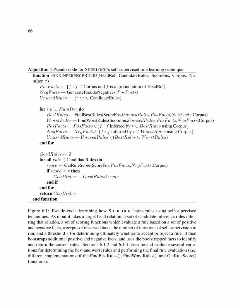
66
Algorithm 1 Pseudo-code for SHERLOCK’s self-supervised rule learning technique.function FINDINFERENCERULES(HeadRel, CandidateRules, ScoreFns, Corpus, Nu-mIter, τ )
PosFacts← {f : f ∈ Corpus and f is a ground atom of HeadRel}NegFacts← GeneratePseudoNegatives(PosFacts)UnusedRules← {r : r ∈ CandidateRules}
for i ∈ 1..NumIter doBestRules← FindBestRules(ScoreFns,UnusedRules,PosFacts,NegFacts,Corpus)WorstRules← FindWorstRules(ScoreFns,UnusedRules,PosFacts,NegFacts,Corpus)PosFacts← PosFacts ∪{f : f inferred by r ∈ BestRules using Corpus}NegFacts← NegFacts ∪{f : f inferred by r ∈WorstRules using Corpus}UnusedRules← UnusedRules \ (BestRules ∪WorstRules)
end for
GoodRules← ∅for all rule ∈ CandidateRules do
score← GetRuleScore(ScoreFns,PosFacts,NegFacts,Corpus)if score ≥ τ then
GoodRules← GoodRules ∪ ruleend if
end forreturn GoodRules
end function
Figure 6.1: Pseudo-code describing how SHERLOCK learns rules using self-supervisedtechniques. As input it takes a target head relation, a set of candidate inference rules infer-ring that relation, a set of scoring functions which evaluate a rule based on a set of positiveand negative facts, a corpus of observed facts, the number of iterations of self-supervision torun, and a threshold τ for determining ultimately whether to accept or reject a rule. It thenbootstraps additional positive and negative facts, and uses the bootstrapped facts to identifyand return the correct rules. Sections 6.1.2 and 6.1.3 describe and evaluate several varia-tions for determining the best and worst rules and performing the final rule evaluation (i.e.,different implementations of the FindBestRules(), FindWorstRules(), and GetRuleScore()functions).
67
modified version of SHERLOCK labels all facts deduced from the ‘good’ and ‘bad’ rules,
rather than a subset of those facts. This helps bootstrapping since at each iteration the
system can label a large number of facts, but it has the risk of exacerbating errors if an
incorrect or unsound rule is selected early on.
This is a self-supervised algorithm since SHERLOCK bootstraps from observed (but not
manually validated) facts, rather than requiring labeled data. As such, even with these
modifications SHERLOCK-HOLMES can scale to open domains. Finally, we note that this
rule learning method assumes that the corpus (evidence) is fixed, and does not consider
inference of or interactions with other rules. Avoiding these computations of longer-range
inferences is done primarily for efficiency, but in preliminary tests it seems to improve
precision as well. The intuition for this effect is that deeper inferences tend to be more
susceptible to errors in our corpus, as many of the inferences are based on noisy facts.
Considering joint interactions between rules is an important item of future work.
6.1.2 Methodology for Evaluation
To evaluate the effects of self-supervised rule learning in Algorithm 1, we need to determine
three things: (1) what rule scoring functions should we use, (2) how do we define the
FindBestRules() and FindWorstRules() functions, and (3) how do we determine the final
rule score?
To answer the first question, in this work we will use the two best rule scoring functions
found previously: SHERLOCK’s statistical relevance + statistical significance rule scoring
function (Section 3.5) and the M-Estimate rule scoring function [16]. These two scoring
functions focus on different features of the problem. SHERLOCK’s rule scoring function
uses only positive examples, but makes use of object frequency (e.g., NewYork is more
likely to appear in an extraction than LasCruces). On the other hand, the M-Estimate
rule scoring function leverages negative examples. Since the rule scoring functions exploit
different features and make qualitatively different errors, we would expect that combining
both will lead to improved results.
68
We consider four methods of combining the scoring functions: a simple, self-training
variant and three others inspired by co-training and co-boosting. At every iteration in the
algorithm the rules are scored as described below, using the scoring functions with the
currently bootstrapped set of positive and negative examples. The four ways of combining
the scoring functions are:
Self-training. This method considers the best and worst rules according to a single scor-
ing function (SHERLOCK’s or M-Estimate), ignoring the other one. At every itera-
tion the FindBestRules() function returns the single highest scoring rule and the Find-
WorstRules() returns the single lowest scoring rule according to the scoring function
used.
Co-training. This method considers the two scoring functions independently from each
other, selecting the best and worst rules according to each function individually. At
every iteration the FindBestRules() function returns two rules - the highest scoring rule
according to the M-Estimate scoring function and the highest scoring rule according to
SHERLOCK’s scoring function. Similarly, the FindWorstRules() function returns the two
rules scoring lowest according to M-Estimate and SHERLOCK, independently.
Agreement Co-boosting. This method considers the two scoring functions jointly. This
matches the intuition that if a rule scores highly according to both scoring functions,
it is probably a good rule, and if a rule scores low according to both scoring func-
tions, it is probably a bad rule. Since the two scoring functions give scores in signif-
icantly different scales, it is unclear how to directly combine the scores. Therefore,
we rank the rules in order of decreasing score according to each of the scoring func-
tions, and use the rank information as a proxy for rule quality. Then at every itera-
tion the FindBestRules() function returns the two rules with the lowest sum of ranks:
argminrule
[rankM−Estimate(rule)+rankSherlock(rule)] (i.e., rules which both scoring func-
tions agree are good). Similarly, the FindWorstRules() function returns the two rules
69
with the highest sum of ranks: argmaxrule
[rankM−Estimate(rule) + rankSherlock(rule)]
(i.e., rules which both scoring functions agree are bad).
Disagreement Co-boosting. This method is similar to agreement co-boosting, but chooses
the worst rules as the ones where the the two rule scoring functions most disagree. In-
tuitively, the goal of this technique is to find a better set of negative examples by using
one rule scoring function to identify and correct the mistakes of the other. To do so,
this technique makes the assumption that if one rule scoring function determines that
a rule is incorrect, then the rule is probably incorrect. This assumption is strong, but
not unreasonable, since most rules are incorrect. The FindBestRules() function uses
agreement between the scoring functions as with agreement co-boosting. However,
the FindWorstRules() function returns two rules having largest difference in rank. I.e.,
argmaxrule
[rankM−Estimate(rule)−rankSherlock(rule)] and argmaxrule
[rankSherlock(rule)−
rankM−Estimate(rule)]
After several rounds of bootstrapping additional positive and negative facts, Algo-
rithm 1 uses the bootstrapped facts to evaluate candidate rules. In the experiments be-
low, we compare three methods for this final evaluation of the rules. (1) using a thresh-
old on SHERLOCK’s rule scoring function, (2) using a threshold on the M-Estimate rule
scoring function, and (3) using a simple ensemble by voting over both scoring functions:
scoreM−Estimate > τm ∧ scoreSherlock > τs. We expect the improved set of positive and
negative examples will increase the performance of M-Estimate, and furthermore that the
additional positive examples will also improve SHERLOCK by providing more accurate
probability estimates for computing statistical relevance and statistical significance. Fi-
nally, we expect that the voting method will lead to improved precision, but at the cost of
recall.
We consider all twelve variations of the four score function combinations and three
final rule scoring methods in the evaluation section below. Finally, we note that although
it is likely that the best rules selected during bootstrapping will be in the final set, it is by
70
no means guaranteed. In some cases there is still insufficient confidence in some of these
rules, even with the additional bootstrapped facts.
6.1.3 Evaluation
Qualitatively, self-supervised rule learning overcomes many of the limitations from the ini-
tial version of SHERLOCK. In many cases the bootstrapped facts provide sufficient support
for rules which previously had only sparse evidence. For example, several variations accept
useful rules that were missing before, such as
Prevents(food, disease) : −Provides(food, nutrient)
∧ Prevents(nutrient, disease);
Additionally, the bootstrapped examples help the system avoid many unsound inference
rules that were accepted previously. For example, the M-Estimate scoring function previ-
ously accepted the unsound rule
IsHeadquarteredIn(company, city) : −IsHeadquarteredIn(company, place)
∧ IsLocatedIn(city, place);
but correctly rejects it using the bootstrapped negative examples.
Unfortunately, in some cases incorrect rules which were previously rejected are ac-
cepted. For example, in some variations the rule
Prevents(food, disease) : −Causes(food, disease);
is learned, whereas it was correctly rejected before.
Qualitatively, the overall trend is that the rules learned tend to be more bimodal. In
the initial version of SHERLOCK there was a mix of correct and incorrect rules learned for
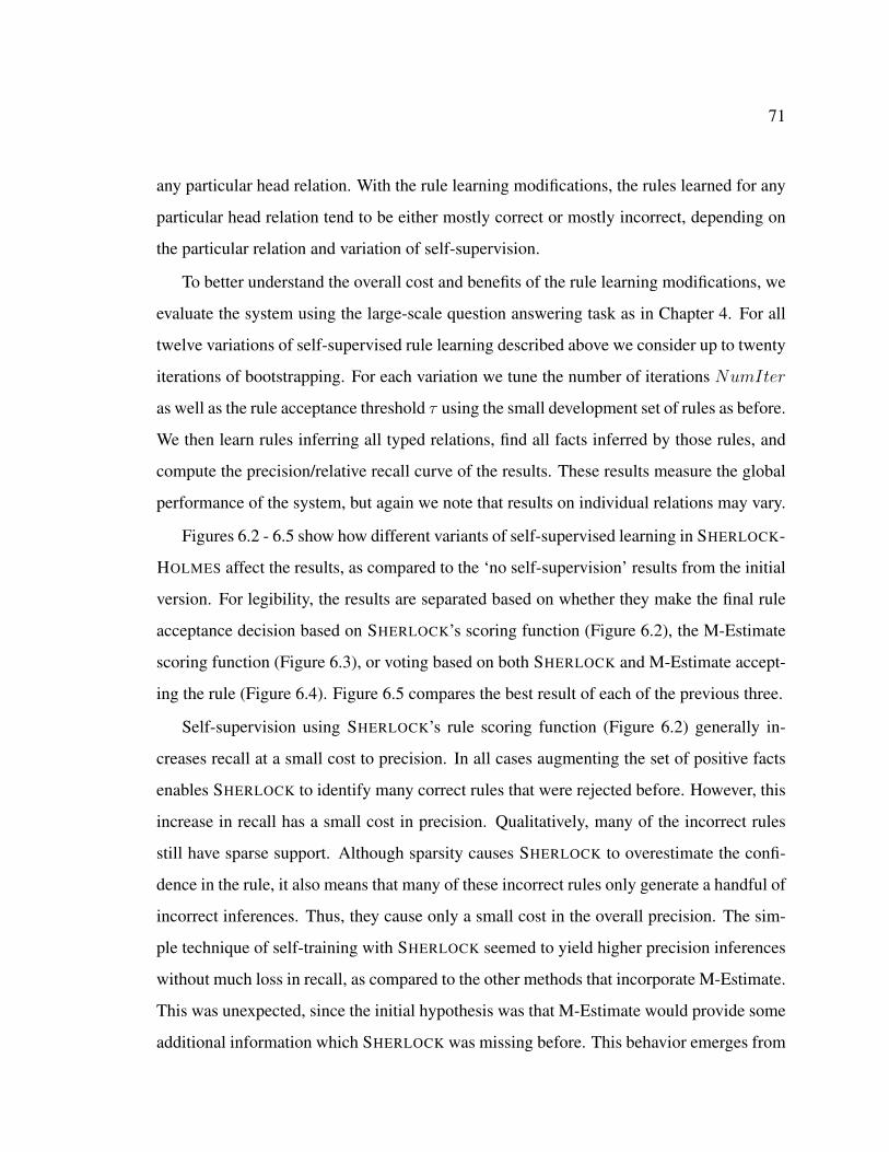
71
any particular head relation. With the rule learning modifications, the rules learned for any
particular head relation tend to be either mostly correct or mostly incorrect, depending on
the particular relation and variation of self-supervision.
To better understand the overall cost and benefits of the rule learning modifications, we
evaluate the system using the large-scale question answering task as in Chapter 4. For all
twelve variations of self-supervised rule learning described above we consider up to twenty
iterations of bootstrapping. For each variation we tune the number of iterations NumIter
as well as the rule acceptance threshold τ using the small development set of rules as before.
We then learn rules inferring all typed relations, find all facts inferred by those rules, and
compute the precision/relative recall curve of the results. These results measure the global
performance of the system, but again we note that results on individual relations may vary.
Figures 6.2 - 6.5 show how different variants of self-supervised learning in SHERLOCK-
HOLMES affect the results, as compared to the ‘no self-supervision’ results from the initial
version. For legibility, the results are separated based on whether they make the final rule
acceptance decision based on SHERLOCK’s scoring function (Figure 6.2), the M-Estimate
scoring function (Figure 6.3), or voting based on both SHERLOCK and M-Estimate accept-
ing the rule (Figure 6.4). Figure 6.5 compares the best result of each of the previous three.
Self-supervision using SHERLOCK’s rule scoring function (Figure 6.2) generally in-
creases recall at a small cost to precision. In all cases augmenting the set of positive facts
enables SHERLOCK to identify many correct rules that were rejected before. However, this
increase in recall has a small cost in precision. Qualitatively, many of the incorrect rules
still have sparse support. Although sparsity causes SHERLOCK to overestimate the confi-
dence in the rule, it also means that many of these incorrect rules only generate a handful of
incorrect inferences. Thus, they cause only a small cost in the overall precision. The sim-
ple technique of self-training with SHERLOCK seemed to yield higher precision inferences
without much loss in recall, as compared to the other methods that incorporate M-Estimate.
This was unexpected, since the initial hypothesis was that M-Estimate would provide some
additional information which SHERLOCK was missing before. This behavior emerges from
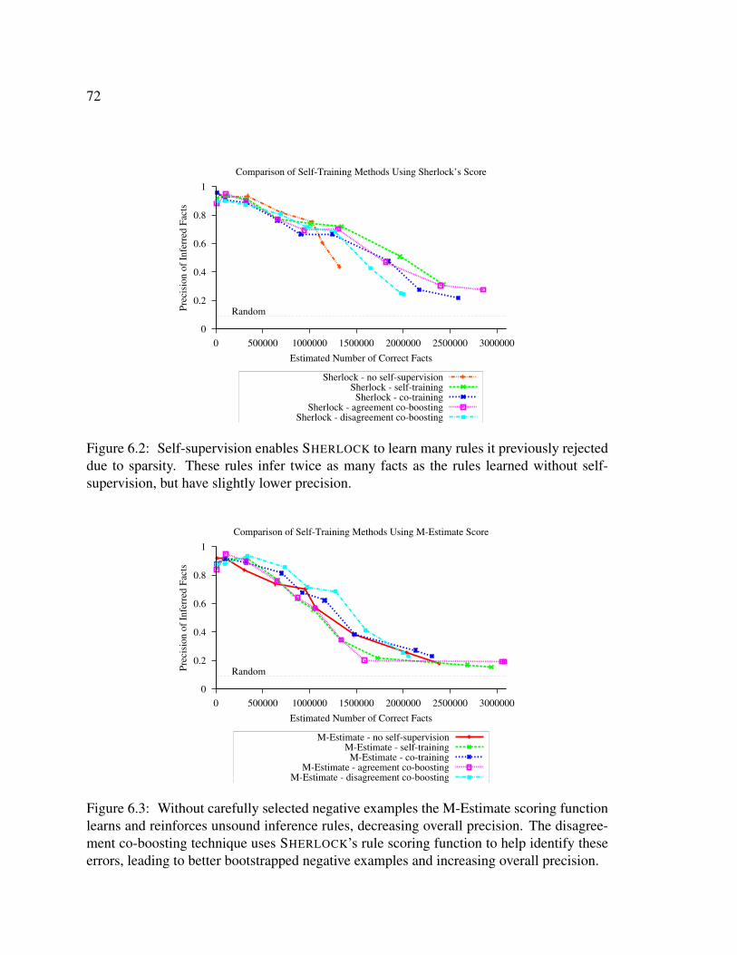
72
0
0.2
0.4
0.6
0.8
1
0 500000 1000000 1500000 2000000 2500000 3000000
Pre
cisi
on
of
Infe
rred
Fac
ts
Estimated Number of Correct Facts
Comparison of Self-Training Methods Using Sherlock’s Score
Sherlock - no self-supervisionSherlock - self-training
Sherlock - co-trainingSherlock - agreement co-boosting
Sherlock - disagreement co-boosting
Random
Figure 6.2: Self-supervision enables SHERLOCK to learn many rules it previously rejecteddue to sparsity. These rules infer twice as many facts as the rules learned without self-supervision, but have slightly lower precision.
0
0.2
0.4
0.6
0.8
1
0 500000 1000000 1500000 2000000 2500000 3000000
Pre
cisi
on
of
Infe
rred
Fac
ts
Estimated Number of Correct Facts
Comparison of Self-Training Methods Using M-Estimate Score
M-Estimate - no self-supervisionM-Estimate - self-trainingM-Estimate - co-training
M-Estimate - agreement co-boostingM-Estimate - disagreement co-boosting
Random
Figure 6.3: Without carefully selected negative examples the M-Estimate scoring functionlearns and reinforces unsound inference rules, decreasing overall precision. The disagree-ment co-boosting technique uses SHERLOCK’s rule scoring function to help identify theseerrors, leading to better bootstrapped negative examples and increasing overall precision.
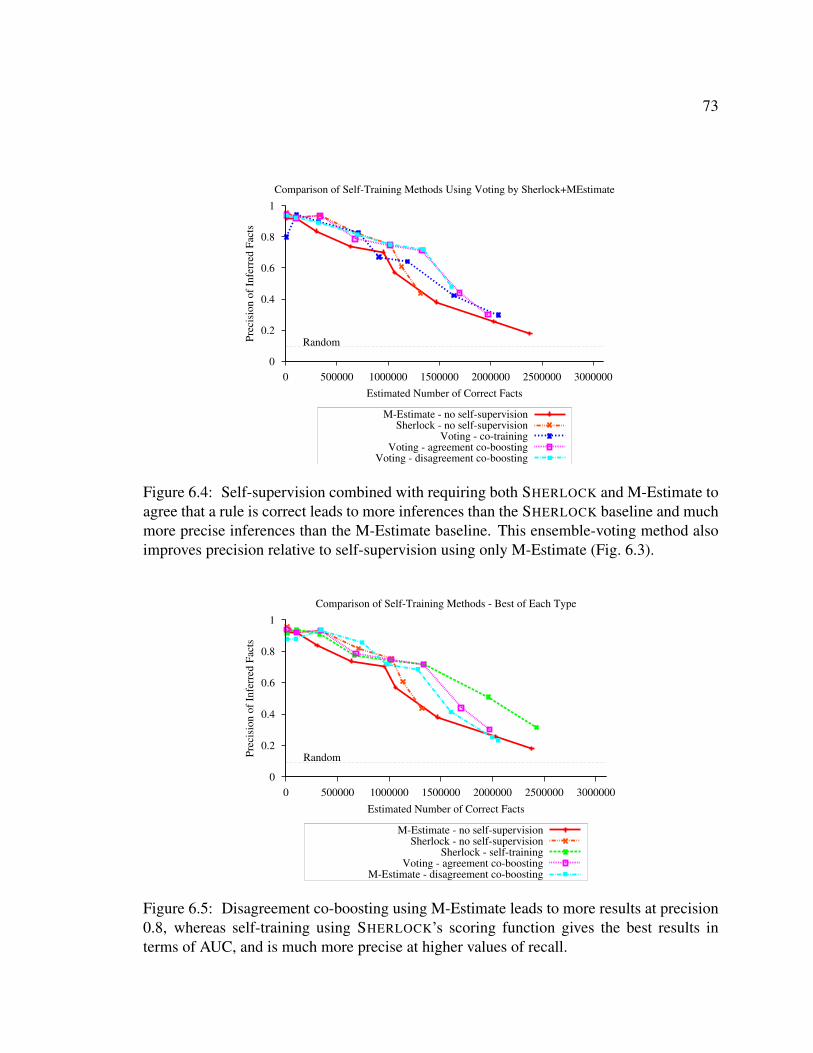
73
0
0.2
0.4
0.6
0.8
1
0 500000 1000000 1500000 2000000 2500000 3000000
Pre
cisi
on o
f In
ferr
ed F
acts
Estimated Number of Correct Facts
Comparison of Self-Training Methods Using Voting by Sherlock+MEstimate
M-Estimate - no self-supervisionSherlock - no self-supervision
Voting - co-trainingVoting - agreement co-boosting
Voting - disagreement co-boosting
Random
Figure 6.4: Self-supervision combined with requiring both SHERLOCK and M-Estimate toagree that a rule is correct leads to more inferences than the SHERLOCK baseline and muchmore precise inferences than the M-Estimate baseline. This ensemble-voting method alsoimproves precision relative to self-supervision using only M-Estimate (Fig. 6.3).
0
0.2
0.4
0.6
0.8
1
0 500000 1000000 1500000 2000000 2500000 3000000
Pre
cisi
on
of
Infe
rred
Fac
ts
Estimated Number of Correct Facts
Comparison of Self-Training Methods - Best of Each Type
M-Estimate - no self-supervisionSherlock - no self-supervision
Sherlock - self-trainingVoting - agreement co-boosting
M-Estimate - disagreement co-boosting
Random
Figure 6.5: Disagreement co-boosting using M-Estimate leads to more results at precision0.8, whereas self-training using SHERLOCK’s scoring function gives the best results interms of AUC, and is much more precise at higher values of recall.
74
the fact that SHERLOCK relies only on positive data. Since M-Estimate has lower precision,
it introduces more errors into the positive facts, which ultimately cause SHERLOCK to have
false confidence in many incorrect rules.
When using the M-Estimate scoring function (Figure 6.3), the results were surprising.
Self-training and agreement co-boosting both yielded overall lower precision results, and
co-training gave only minor improvements. However, the disagreement co-boosting tech-
nique, which uses SHERLOCK’s scoring function to correct rules that M-Estimate is over-
confident in, led to more precise inferences with only a small cost to recall. This behavior
stems from the fact that most of M-Estimate’s errors come from rules which are unsound,
but which also infer a fairly large number of (mostly incorrect) facts. ILP systems typi-
cally use ‘near-miss’ negative examples to help avoid these rules. The negative examples
identified by self-training, co-training, and agreement co-boosting come from rules which
are obviously bad (according to several scoring functions), but unfortunately these rules are
in some sense far from decision boundary. By using information about where M-Estimate
and SHERLOCK disagree, the disagreement co-boosting technique identifies rules which
are much closer to the decision boundary, leading to better, near-miss negative facts. This
helps improve M-Estimate’s precision overall.
Finally, we hoped to further improve the results by accepting only rules that both M-
Estimate and SHERLOCK both agree on (Figure 6.4). Although this improves the results
over those of only using M-Estimate, in general the results are worse than when only using
SHERLOCK. This poor performance seems to be caused by self-supervision introducing
some correlated errors. For example, when an unsound rule is selected as a good rule
during self-supervision, treating its inferences as positive facts causes both M-Estimate and
SHERLOCK to gain confidence in that rule. As such, when voting on the final decision for
that rule, both scoring functions are likely to be confident in it.
Overall, the best results in terms of area-under-the-curve (AUC) come from self-training
using SHERLOCK’s rule scoring function (Figure 6.5). However, in terms of recall at pre-
cision 0.8, the best results come from disagreement co-boosting using M-Estimate (with
75
SHERLOCK’s original, unsupervised method a close second.) These techniques enable the
system to infer an order of magnitude more correct facts than are explicitly extracted,1 and
yields inferences that are 2-4x better than the best case of random guessing.
6.2 Mutual Exclusion Constraints
Another possible way to improve rule learning is to leverage properties of the relations. In
this section we focus on mutual exclusion constraints, as they provide a way of quickly
and compactly specifying a large number of negative examples. The drawback of this
approach is that these constraints must be manually specified. However, for a proof-of-
concept evaluation this is a fairly small amount of supervision, and furthermore there has
been promising research on automatically learning these constraints.
Previous work has demonstrated the utility of such constraints. Quinlan [50] found that
using functionality constraints can improve accuracy and make it faster for an ILP system to
learn rules. The NELL system [8] uses constraints to help guide its information extraction
and rule learning processes. A number of other information extraction systems have found
that using functionality constraints [1] or multiple, mutually exclusive categories [12, 19,
35, 38, 65, 72] improves extraction and avoids semantic drift.
Although typically these constraints are manually specified, there has been some re-
search on learning them automatically. Lin et al. [34] built a system for automatically
identifying functional relations from Web text, Ritter et al. [53] designed a method for au-
tomatically detecting contradictions in Web text, and McIntosh [38] automatically learned
mutual exclusion categories for information extraction. We perform a proof-of-concept
study by manually specifying mutual exclusion constraints in this work, but we would ide-
ally use techniques such as those listed above to automatically discover the constraints.
We consider the following properties providing mutual exclusion:
Functional Relations. In a functional relation each first argument appears with at most
1For the relations used in our tests
76
one distinct second argument (or vise-versa); all other values are illegal. Formally, we
can express this by the constraint:
∀x, y1, y2, R(x, y1) ∧ ¬Equals(y1, y2)⇒ ¬R(x, y2)
(or a similar constraint for a relation that is functional in the second argument).
Antonymy. Relations such as Causes(x, y) and Prevents(x, y) are antonyms of each
other. As such, the facts from one of those relations can be used as negative examples of
the other. Formally, we can express this by the constraint:
∀x, y, R1(x, y)⇒ ¬R2(x, y)
Anti-symmetry. Some relations have a directional property where knowing that the re-
lation occurs from A to B means that the relation does not occur in the other direction
as well (e.g., if comany A acquires company B, then company B does not also acquire
company A). Formally, we can express this by the constraint:
∀x, y, R(x, y)⇒ ¬R(y, x)
Although these properties seem clear logically, there are a number of issues which arise
when using these properties on facts extracted from the Web. Whether or not these prop-
erties hold depend on context, which is often missing in the simple representation of facts
extracted by TEXTRUNNER. For example, the relation IsBasedIn(company, location)
is apparently functional (e.g., a company is based in only one location). However, the facts
IsBasedIn(Amazon, Seattle) and IsBasedIn(Amazon, Washington) are not mutually
exclusive. Furthermore, even with the appropriate type restrictions (e.g.,
IsBasedIn(company, city) ), many apparently functional relations have unextracted tem-
poral context. For example, Boeing was based in Seattle until 2001, when they moved com-
77
pany headquarters to Chicago. TEXTRUNNER contains both IsBasedIn(Boeing, Seattle)
and IsBasedIn(Boeing, Chicago). Similarly, many antonym relations are only mutually
exclusive in a particular temporal context which is typically not extracted. For example,
Beat(team1, team2) and LostTo(team1, team2) are antonyms, but only if we know the
particular game event that is being discussed. Since most rivals have defeated and lost
to each other at some point, both facts are likely to be extracted. Thus, without knowing
which game is being discussed, it is impossible to say whether the two facts are mutually
exclusive.
6.2.1 Evaluating the Utility of Mutual Exclusion Constraints
To study how these mutual exclusion constraints affect rule learning, we first need to iden-
tify a set of relations where the constraints hold. For this experiment we sampled 250 typed
relations at random from the 10,000 identified by SHERLOCK, and manually identified the
mutual exclusion constraints, if any, that applied to each sampled relation. Our sample
contained 51 relations that had at least one applicable mutual exclusion constraint, and
16 relations with multiple mutual exclusion constraints (e.g., CapitalOf(city, state) is
both functional and anti-symmetric.) In our test set, 8 relations have antonyms, 24 are anti-
symmetric, and 35 are functional in either the first or the second argument. Additionally,
we found 36 relations in our sample that were mutual exclusive within a particular temporal
context, but we eliminated these as the extractions do not contain chronologic information.
For relations identified as having antonymy constraints, we manually identified their
antonyms within our corpus. Additionally, to overcome sparsity issues in the anti-symmetric
relations, we augmented them with a small number of synonyms. These synonyms were
only used to generate anti-symmetric, negative examples for rule learning, and were not
used to augment the set of positive examples.
To examine how mutual exclusion constraints affect the quality of the learned rules, we
use the same question-answering task as in prior experiments. SHERLOCK’s rule scoring
function (Section 3.5) was designed to learn rules from only positive examples, so it can not
78
make use of the negative examples implied by the mutual exclusion constraints. We instead
provide these negative examples to the M-Estimate scoring function [16], as it has been
shown to be effective when learning rules with positive and negative training examples.
We compare the overall precision and relative-recall of SHERLOCK-HOLMES when
inferring results for the 51 test relations, using the following rule-learning variants: (1) a
no-inference baseline, (2) inference using the rules learned by SHERLOCK’s rule scoring
function, (3) inference using the rules learned by the M-Estimate scoring function [16], with
negative examples generated randomly as before (Section 4.2), and (4) inference using the
rules learned by the M-Estimate scoring function, but with negative examples generated
from the mutual exclusion constraints.
We found that the mutual exclusion constraints were generating many false negatives,
based on extraction errors, hyperbolic statements, or simply false information. These false
negatives lowered the m-estimate scores for almost all rules when using mutual exclusion
constraints. To counteract this, we lowered the rule acceptance threshold and tuned it with
a small development set as before.2
Figure 6.6 shows how the mutual exclusion constraints affect SHERLOCK-HOLMES’s
results. As is apparent, rules learned accounting for the mutual exclusion constraints are
more accurate than rules learned without them, leading to both higher precision and higher
relative-recalls of facts for the 51 test relations.
The negative examples provided by the mutual exclusion constraints help eliminate
many rules which are unsound, but which have a decent amount of support in the corpus.
For example, without mutual exclusion information, the following rules are learned:
2We examined re-tuning the thresholds from the other scoring methods as well, but found that doing sodecreased their performance on this dataset. As such, we use the thresholds found in prior experiments.
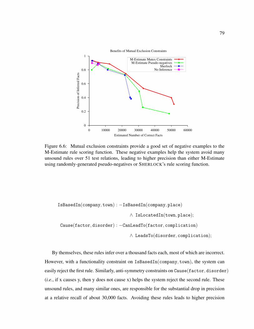
79
0
0.2
0.4
0.6
0.8
1
0 10000 20000 30000 40000 50000 60000
Pre
cisi
on
of
Infe
rred
Fac
ts
Estimated Number of Correct Facts
Benefits of Mutual Exclusion Constraints
M-Estimate Mutex ConstraintsM-Estimate Pseudo-negatives
SherlockNo Inference
Figure 6.6: Mutual exclusion constraints provide a good set of negative examples to theM-Estimate rule scoring function. These negative examples help the system avoid manyunsound rules over 51 test relations, leading to higher precision than either M-Estimateusing randomly-generated pseudo-negatives or SHERLOCK’s rule scoring function.
IsBasedIn(company, town) : −IsBasedIn(company, place)
∧ IsLocatedIn(town, place);
Cause(factor, disorder) : −CanLeadTo(factor, complication)
∧ LeadsTo(disorder, complication);
By themselves, these rules infer over a thousand facts each, most of which are incorrect.
However, with a functionality constraint on IsBasedIn(company, town), the system can
easily reject the first rule. Similarly, anti-symmetry constraints on Cause(factor, disorder)
(i.e., if x causes y, then y does not cause x) helps the system reject the second rule. These
unsound rules, and many similar ones, are responsible for the substantial drop in precision
at a relative recall of about 30,000 facts. Avoiding these rules leads to higher precision
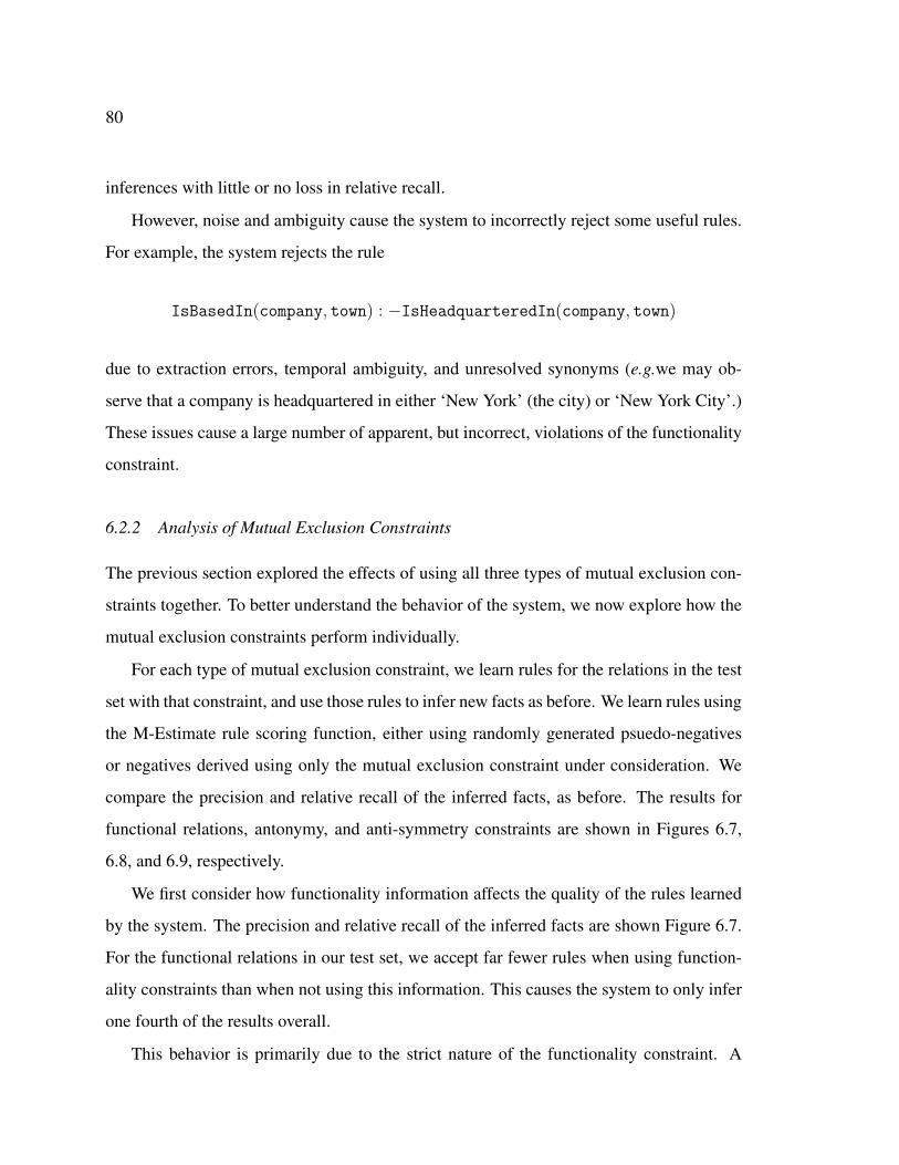
80
inferences with little or no loss in relative recall.
However, noise and ambiguity cause the system to incorrectly reject some useful rules.
For example, the system rejects the rule
IsBasedIn(company, town) : −IsHeadquarteredIn(company, town)
due to extraction errors, temporal ambiguity, and unresolved synonyms (e.g.we may ob-
serve that a company is headquartered in either ‘New York’ (the city) or ‘New York City’.)
These issues cause a large number of apparent, but incorrect, violations of the functionality
constraint.
6.2.2 Analysis of Mutual Exclusion Constraints
The previous section explored the effects of using all three types of mutual exclusion con-
straints together. To better understand the behavior of the system, we now explore how the
mutual exclusion constraints perform individually.
For each type of mutual exclusion constraint, we learn rules for the relations in the test
set with that constraint, and use those rules to infer new facts as before. We learn rules using
the M-Estimate rule scoring function, either using randomly generated psuedo-negatives
or negatives derived using only the mutual exclusion constraint under consideration. We
compare the precision and relative recall of the inferred facts, as before. The results for
functional relations, antonymy, and anti-symmetry constraints are shown in Figures 6.7,
6.8, and 6.9, respectively.
We first consider how functionality information affects the quality of the rules learned
by the system. The precision and relative recall of the inferred facts are shown Figure 6.7.
For the functional relations in our test set, we accept far fewer rules when using function-
ality constraints than when not using this information. This causes the system to only infer
one fourth of the results overall.
This behavior is primarily due to the strict nature of the functionality constraint. A
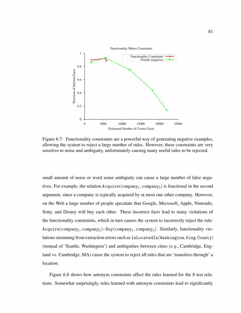
81
0
0.2
0.4
0.6
0.8
1
0 5000 10000 15000 20000 25000
Pre
cisi
on
of
Infe
rred
Fac
ts
Estimated Number of Correct Facts
Functionality Mutex Constraints
Functionality ConstraintsPseudo-negatives
Figure 6.7: Functionality constraints are a powerful way of generating negative examples,allowing the system to reject a large number of rules. However, these constraints are verysensitive to noise and ambiguity, unfortunately causing many useful rules to be rejected.
small amount of noise or word sense ambiguity can cause a large number of false nega-
tives. For example, the relation Acquire(company1, company2) is functional in the second
argument, since a company is typically acquired by at most one other company. However,
on the Web a large number of people speculate that Google, Microsoft, Apple, Nintendo,
Sony, and Disney will buy each other. These incorrect facts lead to many violations of
the functionality constraints, which in turn causes the system to incorrectly reject the rule:
Acquire(company1, company2):-Buy(company1, company2). Similarly, functionality vio-
lations stemming from extraction errors such as IsLocatedIn(Washington, King County)
(instead of ‘Seattle, Washington’) and ambiguities between cities (e.g., Cambridge, Eng-
land vs. Cambridge, MA) cause the system to reject all rules that are ‘transitive-through’ a
location.
Figure 6.8 shows how antonym constraints affect the rules learned for the 8 test rela-
tions. Somewhat surprisingly, rules learned with antonym constraints lead to significantly
82
0
0.2
0.4
0.6
0.8
1
0 2000 4000 6000 8000 10000 12000 14000 16000 18000
Pre
cisi
on
of
Infe
rred
Fac
ts
Estimated Number of Correct Facts
Antonym Mutex Constraints
Antonym ConstraintsPseudo-negatives
Figure 6.8: Using antonym constraints leads to rules which infer many additional facts,but do so at low precision (precision < 0.5). Most of these facts are inferred for a singlehead relation, and stem from sparse negative examples for this relation combined with alower rule acceptance threshold. Including anti-symmetry constraints eliminates most ofthe unsound rules generating these inferences.
more inference than rules learned using only psuedo-negatives. The majority of the new re-
sults results are inferred for a single head relation: CanResultIn(disorder, effect). In
our dataset the antonyms of this relation (e.g., Prevents(disorder, effect) are sparse,
and so only lead to a small number of negative examples. This, combined with a lower
rule acceptance threshold, causes the system to learn many unsound rules that were re-
jected previously due to insufficient support. Fortunately, this problematic relation is also
anti-symmetric. Including the anti-symmetry constraints causes the system to reject these
unsound rules.
Finally, Figure 6.9 examines how anti-symmetry constraints influence the results. These
constraints have a clear benefit, leading to higher precision inferences at all levels of relative
recall. Furthermore, the rules in this case lead to 2-3 times as many facts than were inferred
for the functional relations or the antonym relations.
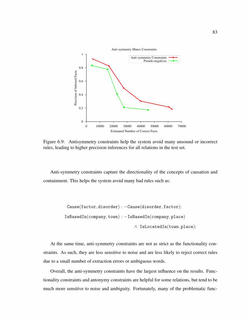
83
0
0.2
0.4
0.6
0.8
1
0 10000 20000 30000 40000 50000 60000 70000
Pre
cisi
on
of
Infe
rred
Fac
ts
Estimated Number of Correct Facts
Anti-symmetry Mutex Constraints
Anti-symmetry ConstraintsPseudo-negatives
Figure 6.9: Antisymmetry constraints help the system avoid many unsound or incorrectrules, leading to higher precision inferences for all relations in the test set.
Anti-symmetry constraints capture the directionality of the concepts of causation and
containment. This helps the system avoid many bad rules such as:
Cause(factor, disorder) : −Cause(disorder, factor);
IsBasedIn(company, town) : −IsBasedIn(company, place)
∧ IsLocatedIn(town, place);
At the same time, anti-symmetry constraints are not as strict as the functionality con-
straints. As such, they are less sensitive to noise and are less likely to reject correct rules
due to a small number of extraction errors or ambiguous words.
Overall, the anti-symmetry constraints have the largest influence on the results. Func-
tionality constraints and antonymy constraints are helpful for some relations, but tend to be
much more sensitive to noise and ambiguity. Fortunately, many of the problematic func-

84
tional or antonym relations are also anti-symmetric, allowing a system using all three types
of mutual exclusion information (as in Section 6.2.1) to outperform a system using only a
single type.
85
Chapter 7
CONCLUSIONS AND FUTURE WORK
The Web has become a vast repository of knowledge, containing information on nearly
any topic imaginable. However, when accessing that knowledge it is typically treated as a
set of independent pages, sentences, or facts. Systems seeking to support more complex
queries that infer information not explicitly stated on the Web must overcome several chal-
lenges. Information on the Web is open-domain (there are an unbounded number of objects
and relations described on the Web), noisy (the Web contains many false statements), am-
biguous (referents are typically not disambiguated), and radically incomplete (many facts
are never explicitly stated). Furthermore, to be useful a system must be able to combine
information gathered across potentially billions of pages, and so its techniques must be
scalable.
The contributions of this dissertation provide solutions which overcome these chal-
lenges. We built and analyzed the SHERLOCK-HOLMES system, one of the first unsu-
pervised systems able to learn first-order, Horn-clause inference rules from open-domain
Web text. SHERLOCK-HOLMES does so by automatically identifying a relatively clean and
well-defined subset of the facts extracted from the Web by TEXTRUNNER, and then evalu-
ating inference rules using a scoring function designed to handle the noise and missing data
prevalent in facts extracted from the Web. The learned rules are useful, allowing the system
to infer three times as many high-quality facts (precision ≥ 0.8) as are in the original sub-
set, and more than five times as many facts overall (albeit at lower precision, but still more
than four times better than random guessing).
To identify correct rules, we defined a novel rule scoring function based on statistical
relevance. We showed that it is effective even when using only a noisy and radically incom-
86
plete collection of facts extracted from the Web. Over a wide variety of relations extracted
from the Web, the rules it learns lead to more accurate inferences than previous rule scoring
functions used in the ILP literature.
This dissertation has also defined the approximately pseudo-functional property (APF),
which characterizes the long-tailed behavior of relations extracted from the Web. We
demonstrated that this property is common within the facts extracted by TEXTRUNNER,
and showed theoretically and empirically that it guarantees SHERLOCK-HOLMES’s run-
time will scale linearly in the size of the corpus and in the number of relations considered.
Thus, SHERLOCK-HOLMES, and other systems using similar techniques, should be able to
scale to the entire Web.
Finally, we examined extensions to SHERLOCK-HOLMES to further improve its results.
Using techniques from self-supervised learning, we demonstrated that using the best and
worst rules to bootstrap additional positive and negative examples allows SHERLOCK to
discover many useful rules that were rejected before due to data sparsity. The additional
rules allow SHERLOCK-HOLMES to infer twice as many facts as before, but with a small
decrease in precision. Additionally, we found that, for the subset of relations where it is ap-
plicable, adding a small amount of supervision in the form of mutual exclusion constraints
can significantly increase SHERLOCK-HOLMES’s precision.
SHERLOCK-HOLMES opens several directions for future work. An important direc-
tion is to consider interactions between multiple rules (i.e., learning and making inferences
at depth greater than one.) Learning rule weights and computing probabilities within the
Markov logic network becomes expensive in this case, as we no longer can do so in closed
form. Additionally, noise becomes a significant challenge with deeper inference. Currently,
a single extraction error or false statement may only lead to a small number of incorrect con-
clusions. However, deriving additional facts based on those incorrect conclusions may lead
to significantly more incorrect results. Addressing these issues is a significant challenge.
A second direction for future work is to include a small amount of supervision into
the system. We demonstrated that mutual exclusion constraints can be useful, but they
87
do not apply to all relations. Instead, it may be useful to have a person validate a subset
of the learned rules, either the best rules or the ones the system is most unsure about.
Techniques from active learning and crowdsourcing may make this a feasible option. The
results of such research would not only explore the question of how this would affect the
system’s results, but also what the most cost-effective ways of gathering information from
crowdsourced workers are.
Another direction for future work would be to examine how SHERLOCK-HOLMES per-
forms on other datasets. The statistical relevance scoring function is useful on facts ex-
tracted from the Web by TEXTRUNNER, but would it be useful on other, cleaner open-
domain datasets such as Freebase1 or Wikipedia? Finally, studying different methods
for identifying classes, instances, typed-relations, and fact extraction should help extend
SHERLOCK-HOLMES to an even broader collection of facts.
The SHERLOCK-HOLMES system presented in this dissertation shows that it is both
possible and useful to infer new facts from information on the Web. This result has a range
of potential uses, from more advanced question-answering systems to enabling machines
better reasoning capabilities over information in the world.
1http://www.freebase.com/
88
BIBLIOGRAPHY
[1] E. Agichtein and L. Gravano. Snowball: Extracting relations from large plain-textcollections. In Procs. of the Fifth ACM International Conference on Digital Libraries,2000.
[2] R. Agrawal, T. Imielinski, and A. Swami. Mining association rules between sets ofitems in large databases. ACM SIGMOD Record, 22(2):207–216, 1993.
[3] R. Agrawal and R. Srikant. Fast algorithms for mining association rules. In Proc.20th Int. Conf. Very Large Data Bases, VLDB, volume 1215, pages 487–499. Citeseer,1994.
[4] M. Banko, M. Cafarella, S. Soderland, M. Broadhead, and O. Etzioni. Open informa-tion extraction from the Web. In Procs. of IJCAI, 2007.
[5] Michele Banko and Oren Etzioni. The tradeoffs between open and traditional relationextraction. In ACL-08: HLT, 2008.
[6] Avrim Blum and Tom Mitchell. Combining labeled and unlabeled data with co-training. In COLT: Proceedings of the Workshop on Computational Learning Theory,Morgan Kaufmann Publishers, pages 92–100, 1998.
[7] Eric Brill, Susan Dumais, and Michele Banko. An analysis of the AskMSR question-answering system. In EMNLP ’02: Proceedings of the ACL-02 conference on Empir-ical methods in natural language processing, pages 257–264, Morristown, NJ, USA,2002. Association for Computational Linguistics.
[8] Andrew Carlson, Justin Betteridge, Bryan Kisiel, Burr Settles, Estevam R. HruschkaJr., and Tom M. Mitchell. Toward an architecture for never-ending language learn-ing. In Proceedings of the Twenty-Fourth Conference on Artificial Intelligence (AAAI2010), 2010.
[9] P. Clark and P. Harrison. Large-scale extraction and use of knowledge from text. InProceedings of the fifth international conference on Knowledge capture, pages 153–160. ACM, 2009.
89
[10] M. Collins and Y. Singer. Unsupervised models for named entity classification. InProceedings of the Joint SIGDAT Conference on Empirical Methods in Natural Lan-guage Processing and Very Large Corpora, pages 189–196, 1999.
[11] M. Craven, D. DiPasquo, D. Freitag, A.K. McCallum, T. Mitchell, K. Nigam, andS. Slattery. Learning to Extract Symbolic Knowledge from the World Wide Web. InProcs. of the 15th Conference of the American Association for Artificial Intelligence,pages 509–516, Madison, US, 1998. AAAI Press, Menlo Park, US.
[12] J.R. Curran, T. Murphy, and B. Scholz. Minimising semantic drift with mutual exclu-sion bootstrapping. In Proceedings of the 10th Conference of the Pacific Associationfor Computational Linguistics, pages 172–180. Citeseer, 2007.
[13] I. Dagan, O. Glickman, and B. Magnini. The PASCAL Recognising Textual Entail-ment Challenge. Proceedings of the PASCAL Challenges Workshop on RecognisingTextual Entailment, pages 1–8, 2005.
[14] Jesse Davis and Pedro Domingos. Deep transfer via second-order markov logic. InICML ’09: Proceedings of the 26th Annual International Conference on MachineLearning, pages 217–224, New York, NY, USA, 2009. ACM.
[15] L. De Raedt and L. Dehaspe. Clausal discovery. Machine Learning, 26(2):99–146,1997.
[16] S. Dzeroski and I. Bratko. Handling noise in inductive logic programming. In Pro-ceedings of the 2nd International Workshop on Inductive Logic Programming, 1992.
[17] C. Elkan and K. Noto. Learning classifiers from only positive and unlabeled data. InProceeding of the 14th ACM SIGKDD international conference on Knowledge dis-covery and data mining, pages 213–220. ACM, 2008.
[18] O. Etzioni, M. Cafarella, D. Downey, S. Kok, A. Popescu, T. Shaked, S. Soderland,D. Weld, and A. Yates. Unsupervised named-entity extraction from the web: Anexperimental study. Artificial Intelligence, 165(1):91–134, 2005.
[19] O. Etzioni, M. Cafarella, D. Downey, A. Popescu, T. Shaked, S. Soderland, D. Weld,and A. Yates. Methods for domain-independent information extraction from the Web:An experimental comparison. In Procs. of the 19th National Conference on ArtificialIntelligence (AAAI-04), pages 391–398, San Jose, California, 2004.
[20] P.A. Flach and N. Lachiche. Confirmation-guided discovery of first-order rules withTertius. Machine Learning, 42(1):61–95, 2001.
90
[21] Y. Freund and R. Schapire. A desicion-theoretic generalization of on-line learning andan application to boosting. In Computational learning theory, pages 23–37. Springer,1995.
[22] A. Gelman. Bayesian data analysis. CRC press, 2004.
[23] M. Genesereth and N. Nilsson. Logical Foundations of Artificial Intelligence. MorganKaufmann Publishers, Inc., Los Altos, CA, 1987.
[24] W.R. Gilks, S. Richardson, and D.J. Spiegelhalter. Introducing markov chain montecarlo. Markov chain Monte Carlo in practice, pages 1–19, 1996.
[25] M. Hearst. Automatic Acquisition of Hyponyms from Large Text Corpora. In Procs.of the 14th International Conference on Computational Linguistics, pages 539–545,Nantes, France, 1992.
[26] R. Hoffmann, S. Amershi, K. Patel, F. Wu, J. Fogarty, and D. S. Weld. Amplifyingcommunity content creation with mixed-initiative information extraction. In ACMSIGCHI (CHI2009), 2009.
[27] T.N. Huynh and R.J. Mooney. Discriminative structure and parameter learning forMarkov logic networks. In Proceedings of the 25th international conference on Ma-chine learning, pages 416–423. ACM, 2008.
[28] Stanley Kok and Pedro Domingos. Learning the structure of markov logic networks.In ICML ’05: Proceedings of the 22nd international conference on Machine learning,pages 441–448, New York, NY, USA, 2005. ACM.
[29] C.C.T. Kwok, O. Etzioni, and D.S. Weld. Scaling question answering to the Web.Proceedings of the 10th international conference on World Wide Web, pages 150–161,2001.
[30] N. Lavrac and S. Dzeroski, editors. Relational Data Mining. Springer-Verlag, Berlin,September 2001.
[31] N. Lawson, K. Eustice, M. Perkowitz, and M.Y. Yildiz. Annotating large emaildatasets for named entity recognition with Mechanical Turk. In NAACL Workshopon Creating Speech and Language Data With Amazons Mechanical Turk, 2010.
[32] D. Lin and P. Pantel. DIRT – Discovery of Inference Rules from Text. In KDD, 2001.
91
[33] D. Lin and P. Pantel. Concept discovery from text. In Proceedings of the 19th Inter-national Conference on Computational linguistics (COLING-02), pages 1–7, 2002.
[34] T. Lin, Mausam, and O. Etzioni. Identifying Functional Relations in Web Text. InProceedings of the 2010 Conference on Empirical Methods in Natural Language Pro-cessing. Association for Computational Linguistics, 2010.
[35] W. Lin, R. Yangarber, and R. Grishman. Bootstrapped Learning of Semantic Classesfrom Positive and Negative Examples. In Procs. of ICML-2003 Workshop on TheContinuum from Labeled to Unlabeled Data, pages 103–111, Washington, D.C, 2003.
[36] B. Liu, W.S. Lee, P.S. Yu, and X. Li. Partially supervised classification of text docu-ments. In machine learning-international workshop and conference, pages 387–394.Citeseer, 2002.
[37] E. McCreath and A. Sharma. ILP with noise and fixed example size: a Bayesianapproach. In Proceedings of the Fifteenth international joint conference on Artificalintelligence-Volume 2, pages 1310–1315. Morgan Kaufmann Publishers Inc., 1997.
[38] T. McIntosh. Unsupervised discovery of negative categories in lexicon bootstrapping.In Proceedings of the 2010 Conference on Empirical Methods in Natural LanguageProcessing, pages 356–365. Association for Computational Linguistics, 2010.
[39] G. Miller, R. Beckwith, C. Fellbaum, D. Gross, and K. Miller. Introduction to Word-Net: An on-line lexical database. International Journal of Lexicography, 3(4):235–312, 1990.
[40] K. Morik. Balanced cooperative modeling. Machine Learning, 11(2):217–235, 1993.
[41] S. Muggleton. Inverse entailment and Progol. New Generation Computing, 13:245–286, 1995.
[42] S. Muggleton. Learning from positive data. Lecture Notes in Computer Science,1314:358–376, 1997.
[43] K. Nigam, A. McCallum, S. Thrun, and T. Mitchell. Text Classification from Labeledand Unlabeled Documents using EM. Machine Learning, 39(2/3):103–134, 2000.
[44] P. Pantel, R. Bhagat, B. Coppola, T. Chklovski, and E. Hovy. ISP: Learning inferentialselectional preferences. In Proceedings of NAACL HLT, volume 7, pages 564–571,2007.
92
[45] Judea Pearl. Probabilistic reasoning in intelligent systems: networks of plausibleinference. Morgan Kaufmann Publishers Inc. San Francisco, CA, USA, 1988.
[46] Mausam Peng Dai and Daniel S. Weld. Decision-theoretic control of crowd-sourcedworkflows. In Proceedings of the Twenty-Fourth Conference on Artificial Intelligence(AAAI 2010), 2010.
[47] M. Pennacchiotti and F.M. Zanzotto. Learning Shallow Semantic Rules for TextualEntailment. Proceedings of RANLP 2007, 2007.
[48] H. Poon and P. Domingos. Unsupervised semantic parsing. In Proceedings of the2009 Conference on Empirical Methods in Natural Language Processing: Volume1-Volume 1, pages 1–10. Association for Computational Linguistics, 2009.
[49] J. R. Quinlan. Learning logical definitions from relations. Machine Learning, 5:239–2666, 1990.
[50] J. R. Quinlan. Learning first-order definitions of functions. Journal of Artificial Intel-ligence Research, 5(1):139–161, 1996.
[51] Philip Resnik. Selectional preference and sense disambiguation. In Proc. of the ACLSIGLEX Workshop on Tagging Text with Lexical Semantics: Why, What, and How?,1997.
[52] M. Richardson and P. Domingos. Markov Logic Networks. Machine Learning, 62(1-2):107–136, 2006.
[53] A. Ritter, D. Downey, S. Soderland, and O. Etzioni. It’s a contradiction—no, it’snot: a case study using functional relations. In Proceedings of the Conference onEmpirical Methods in Natural Language Processing. Association for ComputationalLinguistics, 2008.
[54] D. Roth. On the hardness of approximate reasoning. Artificial Intelligence, 82(1-2):273–302, 1996.
[55] W.C. Salmon, R.C. Jeffrey, and J.G. Greeno. Statistical explanation & statisticalrelevance. Univ of Pittsburgh Pr, 1971.
[56] S. Schoenmackers, J. Davis, O. Etzioni, and D. Weld. Learning First-Order HornClauses from Web Text. In Proceedings of the 2010 Conference on Empirical Methodsin Natural Language Processing, 2010.
93
[57] S. Schoenmackers, O. Etzioni, and D. Weld. Scaling Textual Inference to the Web. InProcs. of EMNLP, 2008.
[58] L.K. Schubert and M.H. Tong. Extracting and evaluating general world knowledgefrom the brown corpus. In Proc. of the HLT/NAACL Workshop on Text Meaning, 2003.
[59] Y. Shinyama and S. Sekine. Preemptive information extraction using unrestrictedrelation discovery. In Procs. of HLT/NAACL, 2006.
[60] P. Singh, T. Lin, E.T. Mueller, G. Lim, T. Perkins, and W. Li Zhu. Open Mind Com-mon Sense: Knowledge acquisition from the general public. Lecture Notes in Com-puter Science, pages 1223–1237, 2002.
[61] R. Snow, D. Jurafsky, and A. Y. Ng. Semantic taxonomy induction from heterogenousevidence. In COLING/ACL 2006, 2006.
[62] R. Snow, B. O’Connor, D. Jurafsky, and A.Y. Ng. Cheap and Fast-But is it Good?Evaluating Non-Expert Annotations for Natural Language Tasks. In Proceedingsof the Conference on Empirical Methods in Natural Language Processing (EMNLP2008), 2008.
[63] F.M. Suchanek, G. Kasneci, and G. Weikum. Yago: A core of semantic knowledge.In Procs. of WWW, 2007.
[64] M. Tatu and D. Moldovan. COGEX at RTE3. In Proceedings of the ACL-PASCALWorkshop on Textual Entailment and Paraphrasing, pages 22–27, 2007.
[65] M. Thelen and E. Riloff. A Bootstrapping Method for Learning Semantic Lexiconsusing Extraction Pattern Contexts. In Procs. of the 2002 Conference on EmpiricalMethods in NLP, pages 214–221, Philadelphia, Pennsylvania, 2002.
[66] J. Ullman. Database and knowledge-base systems. Computer Science Press, 1989.
[67] B. Van Durme and L.K. Schubert. Open knowledge extraction through compositionallanguage processing. In Symposium on Semantics in Systems for Text Processing,2008.
[68] L. von Ahn and L. Dabbish. Labeling images with a computer game. In ACM CHINotes 2004, 2004.
[69] M.P. Wellman, J.S. Breese, and R.P. Goldman. From knowledge bases to decisionmodels. The Knowledge Engineering Review, 7(1):35–53, 1992.
94
[70] F. Wu and D.S. Weld. Autonomously semantifying wikipedia. Proceedings of the six-teenth ACM conference on Conference on information and knowledge management,pages 41–50, 2007.
[71] Fei Wu and Daniel S. Weld. Open information extraction using Wikipedia. In ACL,2010.
[72] R. Yangarber, W. Lin, and R. Grishman. Unsupervised learning of generalized names.In Proceedings of the 19th international conference on Computational linguistics-Volume 1, pages 1–7. Association for Computational Linguistics, 2002.
[73] David Yarowsky. Unsupervised word sense disambiguation rivaling supervised meth-ods. In Meeting of the Association for Computational Linguistics, pages 189–196,1995.
[74] A. Yates and O. Etzioni. Unsupervised resolution of objects and relations on the Web.In Procs. of HLT, 2007.
[75] A. Yates and O. Etzioni. Unsupervised methods for determining object and relationsynonyms on the web. Journal of Artificial Intelligence Research, 34(1):255–296,2009.
[76] J.S. Yedidia, W.T. Freeman, and Y. Weiss. Generalized belief propagation. Advancesin neural information processing systems, pages 689–695, 2001.
[77] H. Yu, J. Han, and K.C.C. Chang. PEBL: positive example based learning for Webpage classification using SVM. In Proceedings of the eighth ACM SIGKDD interna-tional conference on Knowledge discovery and data mining, pages 239–248. ACM,2002.
[78] Jun Zhu, Zaiqing Nie, Xiaojiang Liu, Bo Zhang, and Ji-Rong Wen. Statsnowball: astatistical approach to extracting entity relationships. In WWW ’09: Proceedings ofthe 18th international conference on World wide web, pages 101–110, New York, NY,USA, 2009. ACM.
95
Appendix A
DOWNLOADABLE RESOURCES
We have made the following data available at:
http://www.cs.washington.edu/research/sherlock-hornclauses/
• The complete list of 156 well defined classes used by SHERLOCK (Section 3.2).
• The 1.1M (class, instance) pairs identified by SHERLOCK (Section 3.2). SHERLOCK
uses these to identify interesting typed-relations.
• The complete list of 10,672 typed-relations found by SHERLOCK (Section 3.3).
SHERLOCK learns rules over these typed-relations.
• The complete list of 30,912 rules accepted by SHERLOCK (Having statistical rele-
vance and statistical significance above thresholds, Section 3.5).
• The complete list of 4.9M rules that have the minimum support (s = 2) in the corpus.
SHERLOCK’s rules are a subset of these rules.
The rules files include the statistical relevance, statistical significance, M-Estimate, and
LIME scores, computed over the entire corpus. They also contain the number of facts
observed in the head relation, inferred by the rule body, and the overlap (number of facts
both observed and inferred).
Unfortunately, due to licensing restrictions we are unable to distribute the raw facts.
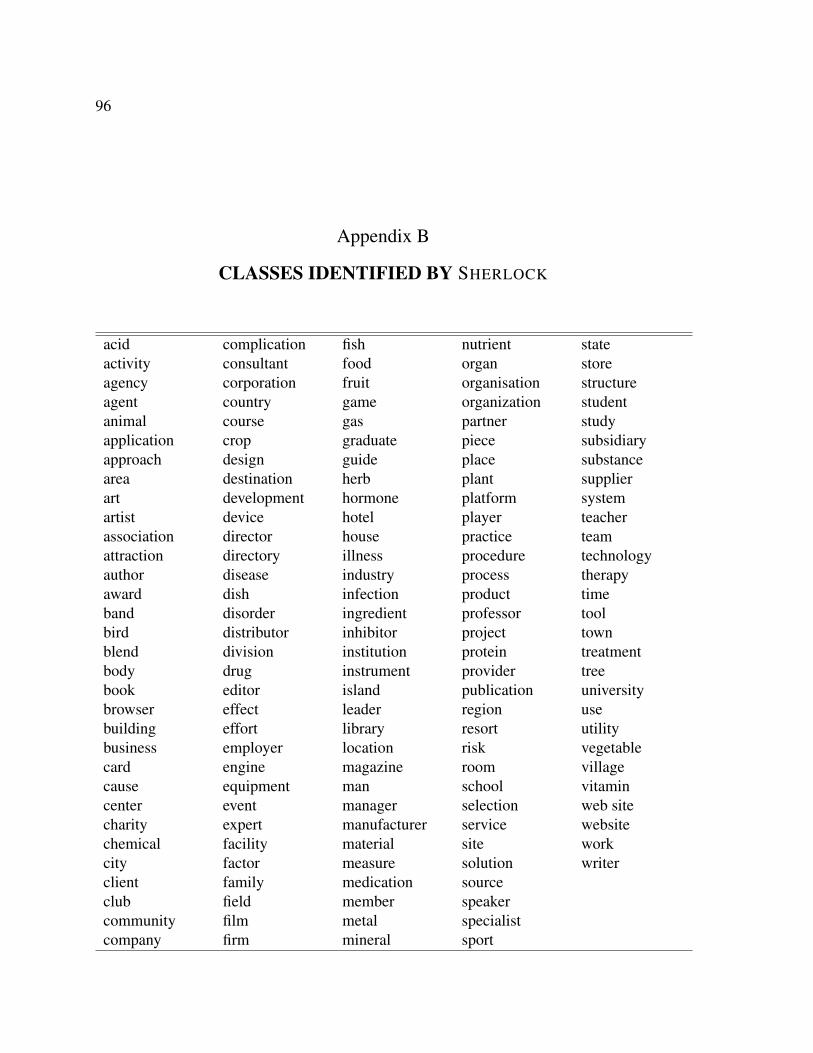
96
Appendix B
CLASSES IDENTIFIED BY SHERLOCK
acid complication fish nutrient stateactivity consultant food organ storeagency corporation fruit organisation structureagent country game organization studentanimal course gas partner studyapplication crop graduate piece subsidiaryapproach design guide place substancearea destination herb plant supplierart development hormone platform systemartist device hotel player teacherassociation director house practice teamattraction directory illness procedure technologyauthor disease industry process therapyaward dish infection product timeband disorder ingredient professor toolbird distributor inhibitor project townblend division institution protein treatmentbody drug instrument provider treebook editor island publication universitybrowser effect leader region usebuilding effort library resort utilitybusiness employer location risk vegetablecard engine magazine room villagecause equipment man school vitamincenter event manager selection web sitecharity expert manufacturer service websitechemical facility material site workcity factor measure solution writerclient family medication sourceclub field member speakercommunity film metal specialistcompany firm mineral sport
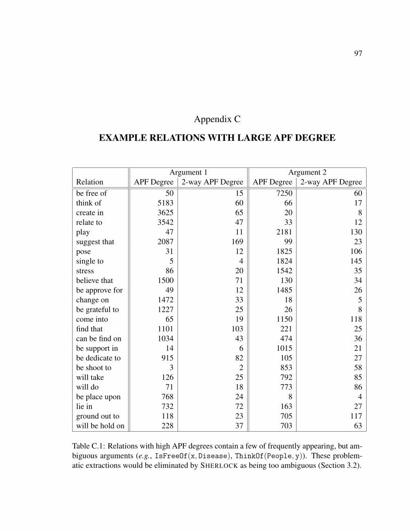
97
Appendix C
EXAMPLE RELATIONS WITH LARGE APF DEGREE
Argument 1 Argument 2Relation APF Degree 2-way APF Degree APF Degree 2-way APF Degreebe free of 50 15 7250 60think of 5183 60 66 17create in 3625 65 20 8relate to 3542 47 33 12play 47 11 2181 130suggest that 2087 169 99 23pose 31 12 1825 106single to 5 4 1824 145stress 86 20 1542 35believe that 1500 71 130 34be approve for 49 12 1485 26change on 1472 33 18 5be grateful to 1227 25 26 8come into 65 19 1150 118find that 1101 103 221 25can be find on 1034 43 474 36be support in 14 6 1015 21be dedicate to 915 82 105 27be shoot to 3 2 853 58will take 126 25 792 85will do 71 18 773 86be place upon 768 24 8 4lie in 732 72 163 27ground out to 118 23 705 117will be hold on 228 37 703 63
Table C.1: Relations with high APF degrees contain a few of frequently appearing, but am-biguous arguments (e.g., IsFreeOf(x, Disease), ThinkOf(People, y)). These problem-atic extractions would be eliminated by SHERLOCK as being too ambiguous (Section 3.2).
98
VITA
Stefan Schoenmackers received a B.S. degree in Computer Engineering and a B.A. de-
gree in Mathematics from the University of California at San Diego in 2004. He continued
his studies at the University of Washington, where he was co-advised by Oren Etzioni and
Dan Weld. While conducting his studies he was supported by a National Science Foun-
dation fellowship, and was awarded the Bob Bandes Memorial Award for Excellence in
Teaching. He received an M.S. degree in 2006, and a Ph.D. in 2011, both in Computer
Science from the University of Washington.