Inference of global clusters from locally distributed datadept.stat.lsa.umich.edu/~xuanlong/Papers/nguyen-ba-10.pdf · Bayesian Analysis (2010) 5, Number 4, pp. 817–846 Inference

Bayesian Analysis (2010) 5, Number 4, pp. 817–846

Inference of global clusters from locally

distributed data

XuanLong Nguyen∗

Abstract. We consider the problem of analyzing the heterogeneity of cluster-ing distributions for multiple groups of observed data, each of which is indexedby a covariate value, and inferring global clusters arising from observations ag-gregated over the covariate domain. We propose a novel Bayesian nonparametricmethod reposing on the formalism of spatial modeling and a nested hierarchy ofDirichlet processes. We provide an analysis of the model properties, relating andcontrasting the notions of local and global clusters. We also provide an efficientinference algorithm, and demonstrate the utility of our method in several data ex-amples, including the problem of object tracking and a global clustering analysisof functional data where the functional identity information is not available.

Keywords: global clustering, local clustering, nonparametric Bayes, hierarchical Dirichlet

process, Gaussian process, graphical model, spatial dependence, Markov chain Monte Carlo,

model identifiability

1 Introduction

In many applications it is common to separate observed data into groups (populations)indexed by some covariate u. A particularly fruitful characterization of grouped datais the use of mixture distributions to describe the populations in terms of clusters ofsimilar behaviors. Viewing observations associated with a group as local data, and theclusters associated with a group as local clusters, it is often of interest to assess howthe local heterogeneity is described by the changing values of covariate u. Moreover,in some applications the primary interest is to extract some sort of global clusteringpatterns that arise out of the aggregated observations.

Consider, for instance, a problem of tracking multiple objects moving in a geograph-ical area. Using covariate u to index the time point, at a given time point u we areprovided with a snapshot of the locations of the objects, which tend to be grouped intolocal clusters. Over time, the objects may switch their local clusters. We are not reallyinterested in the movement of each individual object. It is the paths over which thelocal clusters evolve that are our primary interest. Such paths are the global clusters.Note that the number of global and local clusters are unknown, and are to be inferreddirectly from the locally observed groups of data.

The problem of estimating global clustering patterns out of locally observed groupsof data also arises in the context of functional data analysis where the functional identityinformation is not available. By the absence of functional identity information, we mean

∗Department of Statistics, University of Michigan, Ann Arbor, MI, mailto:[email protected]

c© 2010 International Society for Bayesian Analysis DOI:10.1214/10-BA529

818 Nested hierarchical Dirichlet processes

the data are not actually given as a collection of sampled functional curves (even if suchfunctional curves exist in reality or conceptually), due to confidentiality constraints orthe impracticality of matching the identity of individual functional curves. As anotherexample, the progesterone hormone behaviors recorded by a number of women on agiven day in their monthly menstrual cycle is associated with a local group, whichare clustered into typical behaviors. Such local clusters and the number of clustersmay evolve throughout the monthly cycle. Moreover, aggregating the data over daysin the cycle, there might exist one or more typical monthly (“global” trend) hormonebehaviors due to contraception or medical treatments. These are the global clusters.Due to privacy concern, the subject identity of the hormone levels are neither known normatched across the time points u. In other words, the data are given not as a collectionof hormone curves, but as a collection of hormone levels observed over time.

In the foregoing examples, the covariate u indexes the time. In other applications,the covariate might index geographical locations where the observations are collected.More generally, observations associated with different groups may also be of differentdata types. For instance, consider the assets of a number of individuals (or countries),where the observed data can be subdivided into holdings according to different currencytypes (e.g., USD, gold, bonds). Here, each u is associated with a currency type, anda global cluster may be taken to represent a typical portforlio of currency holdings bya given individual. In view of a substantial existing body of work drawing from thespatial statistics literature that we shall describe in the sequel, throughout this paper acovariate value u is sometimes referred to as a spatial location unless specified otherwise.Therefore, the dependence on varying covariate values u of the local heterogeneity ofdata is also sometimes referred to as the spatial dependence among groups of datacollected at varying local sites.

We propose in this paper a model-based approach to learning global clusters fromlocally distributed data. Because the number of both global and local clusters areassumed to be unknown, and because the local clusters may vary with the covariate u,a natural approach to handling this uncertainty is based on Dirichlet process mixturesand their variants. A Dirichlet process DP(α0, G0) defines a distribution on (random)probability measures, where α0 is called the concentration parameter, and parameterG0 denotes the base probability measure or centering distribution [ Ferguson 1973]. Arandom draw G from the Dirichlet process (DP) is a discrete measure (with probability1), which admits the well-known “stick-breaking” representation [ Sethuraman 1994]:

G =

∞∑

k=1

πkδφk, (1)

where the φk’s are independent random variables distributed according to G0, δφkde-

notes an atomic distribution concentrated at φk, and the stick breaking weights πk arerandom and depend only on parameter α0. Due to the discrete nature of the DP real-izations, Dirichlet processes and their variants have become an effective tool in mixturemodeling and learning of clustered data. The basic idea is to use the DP as a prior on themixture components in a mixture model, where each mixture component is associatedwith an atom in G. The posterior distribution of the atoms provides the probabil-

X. Nguyen 819

ity distribution on mixture components, and also yields a probability distribution ofpartitions of the data. The resultant mixture model, generally known as the Dirichletprocess mixture, was pioneered by the work of [ Antoniak (1974)] and subsequentiallydeveloped by many others (e.g., [ Lo 1984; Escobar and West 1995; MacEachern andMueller 1998]).

A Dirichlet process (DP) mixture can be utilized to model each group of obser-vations, so a key issue is how to model and assess the local heterogeneity among acollection of DP mixtures. In fact, there is an extensive literature in Bayesian non-parametrics that focuses on coupling multiple Dirichlet process mixture distributions(e.g., [ MacEachern (1999); Mueller et al. (2004); DeIorio et al. (2004); Ishwaran andJames (2001); Teh et al. (2006)]). A common theme has been to utilize the Bayesianhierarchical modeling framework, where the parameters are conditionally independentdraws from a probability distribution. In particular, suppose that the u-indexed groupis modeled using a mixing distribution Gu. We highlight the hierarchical Dirichlet pro-cess (HDP) introduced by [ Teh et al. (2006)], a framework that we shall subsequentiallygeneralize, which posits that Gu|α0, G0 ∼ DP(α0, G0) for some base measure G0 andconcentration parameter α0. Moreover, G0 is also random, and is distributed accord-ing to another DP: G0|γ,H ∼ DP(γ,H). The HDP model and other aforementionedwork are inadequate for our problem, because we are interested in modeling the linkageamong the groups not through the exchangeability assumption among the groups, butthrough the more explicit dependence on changing values of a covariate u.

Coupling multiple DP-distributed mixture distributions can be described undera general framework outlined by [ MacEachern (1999)]. In this framework, a DP-distributed random measure can be represented by the random “stick” and “atom” ran-dom variables (see Eq. (1)), which are general stochastic processes indexed by u ∈ V .Starting from this representation, there are a number of proposals for co-varying in-finite mixture models [ Duan et al. 2007; Petrone et al. 2009; Rodriguez et al. 2010;Dunson 2008; Nguyen and Gelfand 2010]. These proposals were designed for functionaldata only, i.e., where the data are given as a collection of sampled functions of u, andthus not suitable for our problem, because functional identity information is assumedunknown in our setting. In this regard, the work of [ Griffin and Steel (2006); Dunsonand Park (2008); Rodriguez and Dunson (2009)] are somewhat closer to our setting.These authors introduced spatial dependency of the local DP mixtures through thestick variables in a number of interesting ways, while [ Rodriguez and Dunson (2009)]additionally considered spatially varying atom variables, resulting in a flexible model.These work focused mostly on the problem of interpolation and prediction, not cluster-ing. In particular, they did not consider the problem of inferring global clusters fromlocally observed data groups, which is our primary goal.

To draw inferences about global clustering patterns from locally grouped data, inthis paper we will introduce an explicit notion of and model for global clusters, throughwhich the dependence among locally distributed groups of data can be described. Thisallows us to not only assess the dependence of local clusters associated with multiplegroups of data indexed by u, but also to extract the global clusters that arise fromthe aggregated observations. From the outset, we use a spatial stochastic process, and


more generally a graphical model H indexed over u ∈ V to characterize the centeringdistribution of global clusters. Spatial stochastic process and graphical models are ver-satile and customary choices for modeling of multivariate data [ Cressie 1993; Lauritzen1996; Jordan 2004]. To “link” global clusters to local clusters, we appeal to a hierar-chical and nonparametric Bayesian formalism: The distribution Q of global clusters israndom and distributed according to a DP: Q|H ∼ DP(γ,H). For each u, the distri-bution Gu of local clusters is assumed random, and is distributed according to a DP:

Gu|Qindep∼ DP(αu, Qu), where Qu denotes the marginal distribution at u induced by the

stochastic process Q. In other words, in the first stage, the Dirichlet process Q providessupport for global atoms, which in turn provide support for the local atoms of lowerdimensions for multiple groups in the second stage. Due to the use of hierarchy andthe discreteness property of the DP realizations, there is sharing of global atoms acrossthe groups. Because different groups may share only disjoint components of the globalatoms, the spatial dependency among the groups is induced by the spatial distributionof the global atoms. We shall refer to the described hierarchical specification as thenested Hierarchical Dirichlet process (nHDP) model.

The idea of incorporating spatial dependence in the base measure of Dirichlet pro-cesses goes back to [ Cifarelli and Regazzini (1978); Muliere and Petrone (1993); Gelfandet al. (2005)], although not in a fully nonparametric hierarchical framework as is consid-ered here. The proposed nHDP is an instantiation of the nonparametric and hierarchicalmodeling philosophy eloquently advocated in [ Teh and Jordan (2010)], but there is acrucial distinction: Whereas Teh and Jordan generally advocated for a recursive con-struction of Bayesian hierarchy, as exemplified by the popular HDP [ Teh et al. 2006],the nHDP features a richer nested hierarchy: instead of taking a joint distribution, onecan take marginal distributions of a random distribution to be the base measure toa DP in the next stage of the hierarchy. This feature is essential to bring about therelationship between global clusters and local clusters in our model. In fact, the nHDPgeneralizes the HDP model in the following sense: If H places a prior with probabilityone on constant functions (i.e., if φ = (φu)u∈V ∼ H then φu = φv∀u, v ∈ V ) then thenHDP is reduced to the HDP.

Most closely related to our work is the hybrid DP of [ Petrone et al. (2009)], whichalso considers global and local clustering, and which in fact serves as an inspiration forthis work. Because the hybrid DP is designed for functional data, it cannot be appliedto situations where functional (curve) identity information is not available, i.e., whenthe data are not given as a collection of curves. When such functional id information isindeed available, it makes sense to model the behavior of individual curves directly, andthis ability may provide an advantage over the nHDP. On the other hand, the hybridDP is a rather complex model, and in our experiment (see Section 5), it tends to overfitthe data due to the model complexity. In fact, we show that the nHDP provides amore satisfactory clustering performance for the global clusters despite not using anyfunctional id information, while the hybrid DP requires not only such information, italso requires the number of global clusters (“pure species”) to be pre-specified. It isworth noting that in the proposed nHDP, by not directly modeling the local clusterswitching behavior, our model is significantly simpler from both viewpoints of model

X. Nguyen 821

complexity and computational efficiency of statistical inference.

The paper outline is as follows. Section 2 provides a brief background of Dirichletprocesses, the HDP, and we then proceed to define the nHDP mixture model. Section 3explores the model properties, including a stick-breaking characterization, an analysis ofthe underlying graphical and spatial dependency, a Polya-urn sampling characterization.We also offer a discussion of a rather interesting issue intrinsic to our problem and thesolution, namely, the conditions under which global clusters can be identified based ononly locally grouped data. As with most nonparametric Bayesian methods, inference isan important issue. We demonstrate in Section 4 that the confluence of graphical/spatialwith hierarchical modeling allows for efficient computations of the relevant posteriordistributions. Section 5 presents several experimental results, including a comparisonto a recent approach in the literature. Section 6 concludes the paper.

2 Model formalization

2.1 Background

We start with a brief background on Dirichlet processes [ Ferguson 1973], and then pro-ceed to hierarchical Dirichlet processes [ Teh et al. 2006]. Let (Θ0,B, G0) be a probabilityspace, and α0 > 0. A Dirichlet process DP(α0, G0) is defined to be the distribution of arandom probability measure G over (Θ0,B) such that, for any finite measurable parti-tion (A1, . . . , Ar) of Θ0, the random vector (G(A1), . . . , G(Ar)) is distributed as a finitedimensional Dirichlet distribution with parameters (α0G0(A1), . . . , α0G0(Ar)). α0 isreferred to as the concentration parameter, which governs the amount of variability ofG around the centering distribution G0. A DP-distributed probability measure G isdiscrete with probability one. Moreover, it has a constructive representation due to [Sethuraman (1994)]: G =

∑∞k=1

πkδφk, where (φk)

∞k=1 are iid draws from G0, and δφk

denotes an atomic probability measure concentrated at atom φk. The elements of thesequence π = (πk)

∞k=1 are referred to as “stick-breaking” weights, and can be expressed

in terms of independent beta variables: πk = π′k

∏k−1

l=1(1 − π′

l), where (π′l)

∞l=1 are iid

draws from Beta(1, α0). Note that π satisfies∑∞k=1

πk = 1 with probability one, andcan be viewed as a random probabity measure on the positive integers. For notationalconvenience, we write π ∼ GEM(α0), following [ Pittman (2002)].

A useful viewpoint for the Dirichlet process is given by the Polya urn scheme, whichshows that draws from the Dirichlet process are both discrete and exhibit a clusteringproperty. From a computational perspective, the Polya urn scheme provides a methodfor sampling from the random distribution G, by integrating out G. More concretely,let atoms θ1, θ2, . . . are iid random variables distributed according to G. Because G israndom, θ1, θ2, . . . are exchangeable. [ Blackwell and MacQueen (1973)] showed thatthe conditional distribution of θi given θ1, . . . , θi−1 has the following form:

[θi|θ1, . . . , θi−1, α0, G0] ∼i−1∑

l=1

1

i− 1 + α0

δθl+

α0

i− 1 + α0

G0.


This expression shows that θi has a positive probability of being equal to one of theprevious draws θ1, . . . , θi−1. Moreover, the more often an atom is drawn, the more likelyit is to be drawn in the future, suggesting a clustering property induced by the randommeasure G. The induced distribution over random partitions of {θi} is also known asthe Chinese restaurant process [ Aldous 1985].

A Dirichlet process mixture model utilizes G as the prior on the mixture componentθ. Combining with a likelihood function P (y|θ) = F (y|θ), the DP mixture model is

given as: θi|G ∼ G; yi|θiind∼ F (·|θi). Such mixture models have been studied in the

pioneering work of [ Antoniak (1974)] and subsequentially by a number of authors [Lo 1984; Escobar and West 1995; MacEachern and Mueller 1998], For more recent andelegant accounts on the theories and wide-ranging applications of DP mixture modeling,see [ Hjort et al. (2010)].

Hierarchical Dirichlet Processes. Next, we proceed giving a brief description of thebackground on the HDP formalism of [ Teh et al. (2006)], which is typically motivatedfrom the setting of grouped data. Under this setting, the observations are organized intogroups indexed by a covariate u ∈ V , where V is the index set. Let yu1, yu2, . . . , yunu

be the observations associated with group u. For each u, the {yui}i are assumed tobe exchangeable. This suggests the use of mixture modeling: The yui are assumedidentically and independently drawn from a mixture distribution. Specifically, let θui ∈Θu denote the parameter specifying the mixture component associated with yui. Underthe HDP formalism, Θu is the same space for all u ∈ V , i.e., Θu ≡ Θ0 for all u, and Θ0

is endowed with the Borel σ-algebra of subsets of Θ0. θui is referred to as local factors

indexed by covariate u. Let F (·|θui) denote the distribution of observation yui given thelocal factor θui. Let Gu denote a prior distribution for the local factors (θui)

nu

i=1. Weassume that the local factors θui’s are conditionally independent given Gu. As a resultwe have the following specification:

θui|Guiid∼ Gu; yui|θui

iid∼ F (·|θui), for any u ∈ V ; i = 1, . . . , nu. (2)

Under the HDP formalism, to statistically couple the collection of mixing distribu-tions Gu, we posit that random probability measures Gu are conditionally independent,with distributions given by a Dirichlet process with base probability measure G0:

Gu|α0, G0iid∼ DP(α0, G0).

Moreover, the HDP framework takes a fully nonparametric and hierarchical specifica-tion, by positing that G0 is also a random probability measure, which is distributedaccording to another Dirichlet process with concentration parameter γ and base prob-ability measure H :

G0|γ,H ∼ DP(γ,H).

An interesting property of the HDP is that because Gu’s are discrete random proba-bility measures (with probability one) whose support are given by the support of G0.Moreover, G0 is also a discrete measure, thus the collection of Gu are random discrete

X. Nguyen 823

measures sharing the same countable support. In addition, because the random par-titions induced by the collection of θui within each group u are distributed accordingto a Chinese restaurant process, the collection of these Chinese restaurant processesare statistically coupled. In fact, they are exchangeable, and the distribution for thecollection of such stoschastic processes is known as the Chinese restaurant franchise [Teh et al. 2006].

2.2 Nested hierarchy of DPs for global clustering analysis

Setting and notations. In this paper we are interested in the same setting of groupeddata as that of the HDP that is described by Eq. (2). Specifically, the observationsyu1, yu2, . . . , yunu

within each group u are iid draws from a mixture distribution. Thelocal factor θui ∈ Θu denotes the parameter specifying the mixture component associ-ated with yui. The (θui)

nu

i=1 are iid draws from the mixing distribution Gu.

Implicit in the HDP model is the assumptions that the spaces Θu all coincide,and that random distributions Gu are exchangeble. Both assumptions will be relaxed.Moreover, our goal here is the inference of global clusters, which are associated withglobal factors that lie in the product space Θ :=

∏

u∈V Θu. To this end, Θ is endowedwith a σ-algebra B to yield a measurable space (Θ,B). Within this paper and in thedata illustrations, Θ = R

V , and B corresponds to the Borel σ-algebra of subsets ofRV , Formally, a global factor, which are denoted by ψ or φ in the sequel, is a high

dimensional vector (or function) in Θ whose components are indexed by covariate u.That is, ψ = (ψu)u∈V ∈ Θ, and φ = (φu)u∈V ∈ Θ. As a matter of notations, we alwaysuse i to denote the numbering index for θu (so we have θui). We always use t and k todenote the number index for instances of ψ’s and φ’s, respectively (e.g., ψt and φk).The components of a vector ψt (φk) are denoted by ψut (φuk). We may also use lettersv and w beside u to denote the group indices.

Model description. Our modeling goal is to specify a distribution Q on the globalfactors ψ, and to relate Q to the collection of mixing distributions Gu associated withthe groups of data. Such resultant model shall enable us to infer about the global

clusters associated with a global factor ψ on the basis of data collected locally by thecollection of groups indexed by u. At a high level, the random probability measures Qand the Gu’s are “glued” together under the nonparametric and hierarchical framework,while the probabilistic linkage among the groups are governed by a stochastic processφ = (φu)u∈V indexed by u ∈ V and distributed according to H . Customary choices ofsuch stochastic processes include either a spatial process, or a graphical model H .

Specifically, let Qu denote the induced marginal distribution of ψu. Our modelposits that for each u ∈ V , Gu is a random measure distributed as a DP with con-centration parameter αu, and base probability measure Qu: Gu|αu, Q ∼ DP(αu, Qu).Conditioning on Q, the distributions Gu are independent, and Gu varies around thecentering distribution Qu, with the amount of variability given by αu. The probabilitymeasure Q is random, and distributed as a DP with concentration parameter γ and


base probability measure H : Q|γ,H ∼ DP(γ,H), where H is taken to be a spatialprocess indexed by u ∈ V , or more generally a graphical model defined on the collectionof variables indexed by V . In summary, collecting the described specifications gives thenested Hierarchical Dirichlet process (nHDP) mixture model:

Q|γ,H ∼ DP(γ,H),

Gu|αu, Qindep∼ DP(αu, Qu), for all u ∈ V

θui|Guiid∼ Gu, yui|θui

iid∼ F (·|θui) for all u, i,

As we shall see in the next section, the φk’s, which are draws from H , provide thesupport for global factors ψt ∼ Q, which in turn provide the support for the local factorsθui ∼ Gu. The global and local factors provide distinct representations for both globalclusters and local clusters that we envision being present in data. Local factors θui’sprovide the support for local cluster centers at each u. The global factors ψ in turnprovide the support for the local clusters, but they also provide the support for globalcluster centers in the data, when observations are aggregated across different groups.

Relations to the HDP. Both the HDP and nHDP are instances of the nonparametricand hierarchical modeling framework involving hierarchy of Dirichlet processes [ Teh andJordan 2010]. At a high-level, the distinction here is that while the HDP is a recursivehierarchy of random probability measures generally operating on the same probabilityspace, the nHDP features a nested hierarchy, in which the probability spaces associatedwith different levels in the hierarchy are distinct but related in the following way: theprobability distribution associated with a particular level, say Gu, has support in thesupport of the marginal distribution of a probability distribution (i.e., Q) in the upperlevel in the hierarchy. Accordingly, for u 6= v, Gu and Gv have support in distinctcomponents of vectors ψ. For a more explicit comparison, it is simple to see that ifH places distribution for constant global factors φ with probability one (e.g., for anyφ ∼ H there holds φu = φv∀u, v ∈ V ), then we obtain the HDP of [ Teh et al. (2006)].

3 Model properties

3.1 Stick-breaking representation and graphical or spatial depen-

dency

Given that the multivariate base measure Q is distributed as a Dirichlet process, it canbe expressed using Sethuraman’s stick-breaking representation: Q =

∑∞k=1

βkδφk. Each

atom φk is multivariate and denoted by φk = (φuk : u ∈ V ). The φk’s are independentdraws from H , and β = (βk)

∞k=1 ∼ GEM(γ). The φk’s and β are mutually independent.

The marginal induced by Q at each location u ∈ V is: Qu =∑∞

k=1βkδφuk

. Since eachQu has support at the points (φuk)

∞k=1, each Gu necessarily has support at these points

X. Nguyen 825

H Hu Hv Hw

Q Qu Qv Qw

Gu Gv Gw

θui θvi θwi θui θvi θwi

γ

β

φuk φvk φwk

πu πv πw

∞

Figure 1: Left: The nHDP is depicted as a graphical model, where each unshaded noderepresents a random distribution. Right: A graphical model representation of the nHDPusing the stick-breaking parameterisation.

as well, and can be written as:

Gu =

∞∑

k=1

πukδφuk; Qu =

∞∑

k=1

βkδφuk. (3)

Let πu = (πuk)∞k=1. Since Gu’s are independent given Q, the weights πu’s are

independent given β. Moreover, because Gu|αu, Q ∼ DP(αu, Qu) it is possible to derivethe relationship between weights πu’s and β. Following [ Teh et al. (2006)], if H is non-atomic, it is necessary and sufficient forGu defined by Eq. (3) to satisfy Gu ∼ DP(αuQu)that the following holds: πu ∼ DP(αu, β), where πu and β are interpreted as probabilitymeasures on the set of positive integers.

The connection between the nHDP and the HDP of [ Teh et al. (2006)] can beobserved clearly here: The stick-breaking weights of the nHDP-distributed Gu have thesame distributions as those of the HDP, while the atoms φuk are linked by a graphicalmodel distribution, or more generally a stochastic process indexed by u.

The spatial/graphical dependency given by base measure H induces the dependencybetween the DP-distributed Gu’s. We shall explore this in details by considering specificexamples of H .

Example 1 (Graphical model H). For concreteness, we consider a graphical modelH of three variables φu, φv, φw which are associated with three locations u, v, w ∈ V .Moreover, assume the conditional independence relation: φu ⊥ φw|φv. Let ψ =(ψu, ψv, ψw) be a random draw from Q. Because Q ∼ DP(γ,H), ψ also has distri-bution H once Q is integrated out. Thus, ψu ⊥ ψw|ψv.

At each location u ∈ V , the marginal distribution Qu of variable ψu is randomand Qu|γ,H ∼ DP(γ,Hu). Moreover, in general the Qu’s are mutually dependentregardless of any (conditional) independence relations that H might confer. This factcan be easily seen from Eq. (3). With probability 1, all Qu’s share the same β. It followsthat Qu ⊥ Qw|Qv,β. Because β is random, the conditional independence relation nolonger holds amongQu, Qw, Qv in general. From a modeling standpoint, the dependencyamong the Qu’s is natural for our purpose, as Q provides the distribution for the global


factors associated with the global clusters that we are also interested in inferring.

Turning now to distributions Gu for local factors θui, we note that Gu, Gv, Gw areindependent given Q. Moreover, for each u ∈ V , the support of Gu is the same asthat of Qu (i.e., θui for i = 1, 2, . . . take value among (ψut)

∞t=1). Integrating over

the random Q, for any measurable partition A ⊂ Θu, there holds: E[Gu(A)|H ] =E[E[Gu(A)|Q]|H ] = E[Qu(A)|H ] = Hu(A). In sum, the global factors ψ’s take valuesin the set of (φk)

∞k=1 ∼ H , and provide the support set for the local factors θui’s at each

u ∈ V . The prior means of the local factors θui’s are also derived from the prior meanof the global factors.

Example 2 (Spatial model H). To quantify more detailed dependency among DP-distributed Gu’s, let V be a finite subset of R

r and H be a second-order stochasticprocess indexed by v ∈ V . A customary choice for H is a Gaussian process. In effect,φ = (φu : u ∈ V ) ∼ N(µ,Σ), where the covariance Σ has entries of the exponentialform: ρ(u, v) = σ2 exp−{ω‖u− v‖}.

For any measurable partitions A ⊂ Θu, and B ⊂ Θv, we are interested in expressionsfor variation and correlation measures under Q and Gu’s. Let Huv(A,B) := p(φu ∈A, φv ∈ B|H). Define g(γ) = 1/(γ + 1). Applying stick-breaking representation for Qu,it is simple to derive that:

Proposition 5. For any pair of distinct locations u, v), there holds:

Cov(Qu(A), Qv(B)|H) = g(γ)(Huv(A,B) −Hu(A)Hv(B)), (4)

Var(Qu(A)|H) = g(γ)(Hu(A) −Hu(A)2), (5)

Corr(Qu(A), Qv(B)) :=Cov(Qu(A), Qv(B)|H)

Var(Qu(A)|H)1/2Var(Qv(B)|H)1/2

=(Huv(A,B) −Hu(A)Hv(B))

(Hu(A) −Hu(A)2)1/2(Hv(B) −Hv(B)2)1/2. (6)

For any pair of locations u, v ∈ V , if ‖u − v‖ → ∞, it follows that ρ(u, v) =Cov(φu, φv|H)→ 0. Due to standard properties of Gaussian variables, φu and φv become less dependentof each other, and Huv(A,B) − Hu(A)Hv(B) → 0, so that Corr(Qu(A), Qv(B)) → 0.On the other hand, if u− v → 0, we obtain that Corr(Qu(A), Qv(A)) → 1, as desired.

Turning to distributions Gu’s for the local factors, the following result can be shown:

Proposition 6. For any pair of u, v ∈ V , there holds:

Var(Gu(A)|H) = E[Var(Gu(A)|Q)|H ] + Var(E[Gu(A)|Q]|H)

= (g(γ) + g(αu) − g(γ)g(αu))(Hu(A) −Hu(A)2), (7)

Corr(Gu(A), Gv(B)) =g(γ)Corr(Qu(A), Qv(B)|H)

(g(γ) + g(αu) − g(γ)g(αu))1/2(g(γ) + g(αv) − g(γ)g(αv))1/2.

where g(αu) = 1/(αu + 1).

X. Nguyen 827

Eq. (7) exhibits an interesting decomposition of variance. Note that Var(Gu(A)|H) ≥Var(Qu(A)|H). That is, the variation of a local factor is greater than that of the globalfactor evaluated at the same location, where the extra variation is governed by concen-tration parameter αu. If αu → ∞ so that g(αu) → 0, the local variation at u disappears,with the remaining variation contributed by the global factors only. If αu → 0 so thatg(αu) → 1, the local variation contributed by Gu completely dominates the globalvariation contributed by Qu.

Finally, turning to correlation measures in the two stages in our hierachical model,we note that Corr(Gu(A), Gv(B)|H) ≤ Corr(Qu(A), Qv(B)|H). That is, the correlationacross the locations in V among the distributions Gu’s of the local factors is boundedfrom above by the correlation among the distribution Qu’s for the global factors. Notethat Corr(Gu(A), Gv(B)) vanishes as ‖u− v‖ → ∞. The correlation measure increasesas either αu or αv increases. The dependence on γ is quite interesting. As γ rangesfrom 0 to ∞ so that g(γ) decreases from 1 to 0, and as a result the correlation measureratio Corr(Gu(A), Gv(B))/Corr(Qu(A), Qv(B)) decreases from 1 to 0.

3.2 Polya-urn characterization

The Polya-urn characterization of the canonical Dirichlet process is fully retained by thenHDP. It is also useful in highlighting both local clustering and global clustering aspectsthat are described by the nHDP mixture. In the sequel, the Polya-urn characterizationis given as a sampling scheme for both the global and local factors. Recall that theglobal factors φ1,φ2, . . . are i.i.d. random variables distributed according to H . Wealso introduced random vectors ψt which are i.i.d. draws from Q. Both φk and ψt aremultivariate, denoted by φk = (φuk)u∈V and ψt = (ψut)u∈V . Finally, for each locationu ∈ V , the local factor variables θui are distributed according to Gu.

Note that each ψt is associated with one φk, and each θui is associated with one ψut.Let tui be the index of the ψut associated with the local factor θui, and kt be the indexof the φk associated with the global factor ψt. Let K be the present number of distinctglobal factors φk. The sampling process starts with K = 0 and increases K as needed.We also need notations for counts. We use notation nut to denote the present numberof local factors θul taking value ψut. nu denotes the number of local factors at groupu (which is also the number of observations at group u). nu·k is the number of localfactors at u taking value φuk. Let mu denote the number of factors ψt that providesupports for group u. The notation qk denotes the number of global factors ψt’s takingvalue φk, while q· denotes the total number of global factors ψt’s. To be precise:

nut =∑

i

I(tui = t); nu·k =∑

t

nutI(kt = k); nu =∑

t

nut;

mu =∑

t

I(nut > 0); qk =∑

t

I(kt = k); q· =∑

k

qk.

First, consider the conditional distribution for θui given θu1, θu2, . . . , θu,i−1, and Q,


where the Gu is integrated out:

θui|θu1, . . . , θu,i−1, αu, Q ∼

mu∑

t=1

nuti− 1 + αu

δψut+

αui− 1 + αu

Qu. (8)

This is a mixture, and a realization from this mixture can be obtained by drawing fromthe terms on the right-hand side with probabilities given by the corresponding mixingproportions. If a term in the first summation is chosen, then we set θui = ψut for thechosen t, and let tui = t, and increment nut. If the second term is chosen, then weincrement mu by one, draw ψumu

∼ Qu. In addition, we set θui = ψumu, and tui = mu.

Now we proceed to integrate out Q. Since Q appears only in its role as the distri-bution of the variable ψt, we only need to draw sample ψt from Q. The samples fromQ can be obtained via the conditional distribution of ψt as follows:

ψt|{ψl}l 6=t, γ,H ∼

K∑

k=1

qkq· + γ

δφk+

γ

q· + γH. (9)

If we draw ψt via choosing a term in the summation on the right-hand side of thisequation, we set ψt = φk, and let kt = k for the chosen k, and increment qk. If thesecond term is chosen then we increment K by one, draw φK ∼ H and set ψt = φK ,kjt = K, and qK = 1.

The Polya-urn characterization of the nHDP can be illustrated by the followingculinary metaphor. Suppose that there are three groups of dishes (e.g., appetizer, maincourse and dessert) indexed by u, v and w. View a global factor φk’s as a typical mealbox where each φuk, φvk and φwk is associated with a dish group. In an electic eatery,the dishes are sold in meal boxes, while customers come in, buy dishes and share amongone another according to the following process. A new customer can join either one ofthe three groups of dishes. Upon joining the group, she orders a dish to contribute tothe group, i.e., a local factor θui, based on its popularity within the group. She can alsochoose to order a new dish, but to do so, she needs to order the entire meal box, i.e.a global factor ψt. A meal box is chosen based on its popularity as a whole, across alleating groups.

The “sharing” of global factors (meal box) across indices u can be seen by notingthat the “pool” of present global factors {ψl} has support in the discrete set of globalfactor values φ1,φ2, . . .. Moreover, the spatial (graphical) distribution of the globalfactors induces the spatial dependence among local factors associated with each groupindexed by u. See Fig. 2 for an illustration.

3.3 Model identifiability and complexity

This section investigates the nHDP mixture’s inferential behavior, including issues re-lated to the model identifiability. It is useful to recall that a DP mixture model can beviewed as the infinite limit of finite mixture models [ Neal 1992; Ishwaran and Zarepour

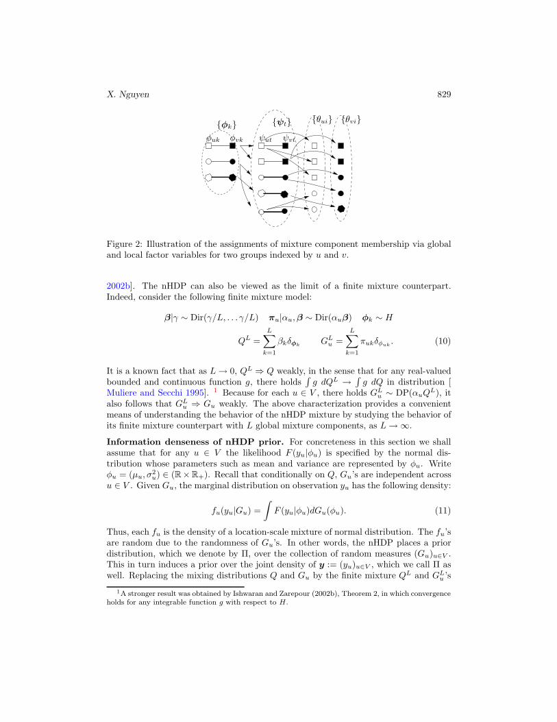
X. Nguyen 829

{φk} {ψt}

φuk φvk ψut ψvt

{θui} {θvi}

Figure 2: Illustration of the assignments of mixture component membership via globaland local factor variables for two groups indexed by u and v.

2002b]. The nHDP can also be viewed as the limit of a finite mixture counterpart.Indeed, consider the following finite mixture model:

β|γ ∼ Dir(γ/L, . . . γ/L) πu|αu,β ∼ Dir(αuβ) φk ∼ H

QL =

L∑

k=1

βkδφkGLu =

L∑

k=1

πukδφuk. (10)

It is a known fact that as L→ 0, QL ⇒ Q weakly, in the sense that for any real-valuedbounded and continuous function g, there holds

∫

g dQL →∫

g dQ in distribution [Muliere and Secchi 1995]. 1 Because for each u ∈ V , there holds GLu ∼ DP(αuQ

L), italso follows that GLu ⇒ Gu weakly. The above characterization provides a convenientmeans of understanding the behavior of the nHDP mixture by studying the behavior ofits finite mixture counterpart with L global mixture components, as L→ ∞.

Information denseness of nHDP prior. For concreteness in this section we shallassume that for any u ∈ V the likelihood F (yu|φu) is specified by the normal dis-tribution whose parameters such as mean and variance are represented by φu. Writeφu = (µu, σ

2u) ∈ (R×R+). Recall that conditionally on Q, Gu’s are independent across

u ∈ V . Given Gu, the marginal distribution on observation yu has the following density:

fu(yu|Gu) =

∫

F (yu|φu)dGu(φu). (11)

Thus, each fu is the density of a location-scale mixture of normal distribution. The fu’sare random due to the randomness of Gu’s. In other words, the nHDP places a priordistribution, which we denote by Π, over the collection of random measures (Gu)u∈V .This in turn induces a prior over the joint density of y := (yu)u∈V , which we call Π aswell. Replacing the mixing distributions Q and Gu by the finite mixture QL and GLu ’s

1A stronger result was obtained by Ishwaran and Zarepour (2002b), Theorem 2, in which convergenceholds for any integrable function g with respect to H.


(as specified by Eq. (10)), we obtain the corresponding marginal density:

fLu (yu|Gu) =

∫

F (yu|φu)dGLu (φu). (12)

Let ΠL to denote the induced prior distribution for {fLu }u∈V . From the above, ΠL ⇒ Πweakly.

We shall show that for each u ∈ V the prior ΠL is information dense in the space offinite mixtures as L → ∞. Indeed, for any group index u, consider any finite mixtureof normals fu,0 associated with mixing distributions Q0 and Gu,0 of the form:

Q0 =

d∑

k=1

βk,0δφk,0, Gu,0 =

d∑

k=1

πuk,0δφuk,0, (13)

Proposition 7. Suppose that the base measure H places positive probability on a rect-

angle containing the support of Q0, then the prior ΠL places a positive probability in

arbitrarily small Kullback-Leibler neighborhood of fu,0 for L sufficiently large. That is,

for any ε > 0, there holds: ΠL(fu : D(fu,0||fu) < ε) > 0 for any sufficiently large L.

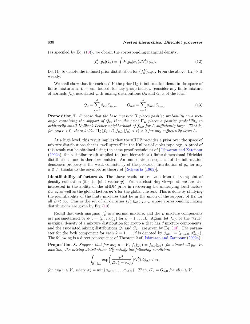
At a high level, this result implies that the nHDP provides a prior over the space ofmixture distributions that is “well spread” in the Kullback-Leibler topology. A proof ofthis result can be obtained using the same proof techniques of [ Ishwaran and Zarepour(2002a)] for a similar result applied to (non-hierarchical) finite-dimensional Dirichletdistributions, and is therefore omitted. An immediate consequence of the informationdenseness property is the weak consistency of the posterior distribution of yu for anyu ∈ V , thanks to the asymptotic theory of [ Schwartz (1965)].

Identifiability of factors φ. The above results are relevant from the viewpoint ofdensity estimation (for the joint vector y). From a clustering viewpoint, we are alsointerested in the ability of the nHDP prior in recovering the underlying local factorsφuk’s, as well as the global factors φk’s for the global clusters. This is done by studyingthe identifiability of the finite mixtures that lie in the union of the support of ΠL forall L < ∞. This is the set of all densities (fLu )u∈V ;L<∞ whose corresponding mixingdistributions are given by Eq. (10).

Recall that each marginal fLu is a normal mixture, and the L mixture componentsare parameterised by φuk = (µuk, σ

2uk) for k = 1, . . . , L. Again, let fu,0 be the “true”

marginal density of a mixture distribution for group u that has d mixture components,and the associated mixing distributions Q0 and Gu,0 are given by Eq. (13). The param-eter for the k-th component for each k = 1, . . . , d is denoted by φuk,0 = (µuk,0, σ

2uk,0).

The following is a direct consequence of Theorem 2 of [Ishwaran and Zarepour (2002a)]:

Proposition 8. Suppose that for any u ∈ V , fu(yu) = fu,0(yu) for almost all yu. In

addition, the mixing distributions GLu satisfy the following condition:∫

R×R+

exp

(

µ2u

2(σ∗u − σu)

)

GLu (dφu) <∞,

for any u ∈ V , where σ∗u = min{σu1,0, . . . , σuk,0}. Then, Gu = Gu,0 for all u ∈ V .

X. Nguyen 831

In other words, this result claims that it is possible to identify all local clustersspecified by φuk and πuk for k = 1, . . . , d, up to the ordering of the mixture componentindex k. A more substantial issue is the identifiability of global factors. Under additionalconditions of “true” global factors φk,0’s, and the distribution of global factors QL, theidentification of global factors φk,0’s is possible. Viewing a global factor φk = (φuk)u∈V(likewise, φk,0) as a function of u ∈ v, a trivial example is that when φk,0 are constantfunctions, and that base measure H (and consequentially QL) places probability 1 onsuch set of functions, then the identifiability of local factors implies the identifiability ofglobal factors. A nontrivial condition is that the “true” global factors φk,0 as a functionof u can be parameterised by a small number of parameters (e.g. a linear function,or an appropriately defined smooth function in u ∈ V ). Then, it is possible that theidentifiability of local factors also implies the identifiability of global factors. An in-depth theoretical treatment of this important issue is beyond the scope of the presentpaper.

The above observations suggest several prudent guidelines for prior specifications(via the base measure H). To ensure good inferential behavior for the local factorsφu’s, it is essential that the base measure Hu places sufficiently small tail probabilitieson both µu and σu. In addition, if it is believed the underlying global factors are smoothfunction in the domain V , placing a very vague prior H over the global factors (suchas a factorial distribution H =

∏

u∈V Hu by assuming the φu are independent acrossu ∈ V ) may not do the job. Instead, an appropriate base measure H that puts most ofits mass on smooth functions is needed. Indeed, these observations are also confirmedby our empirical experiments in Section 5.

4 Inference

In this section we shall describe posterior inference methods for the nested Hierarchi-cal Dirichlet process mixture. We describe two different sampling approaches: The“marginal approach” proceeds by integrating out the DP-distributed random measures,while the “conditional approach” exploits the stick-breaking representation. The formerapproach arises directly from the Polya-urn characterization of the nHDP. However itsimplementation is more involved due to book-keeping of the indices. Within this sectionwe shall describe the conditional approach, leaving the details of the marginal approachto the supplemental material. Both sampling methods draw from the basic featuresof the sampling methods developed for the Hierarchical Dirichlet Process of [Teh et al.(2006)], in addition to the computational issues that arise when high-dimensional globalfactors are sampled.

For the reader’s convenience, we recall key notations and introduce a few more forthe sampling algorithms. tui is the index of the ψut associated with the local factorθui, i.e., θui = ψutui

; and kt is the index of the φk associated with the global factor ψt,i.e., ψt = φkt

. The local and global atoms are related by θui = ψutui= φuktui

. Letzui = ktui

denote the mixture component associated with observation yui. Turning tocount variables, n−ui

ut denotes the number of local atoms θul’s that are associated with


ψt, excluding atom θui. n−uiu·k denotes the number of local atoms θul that such that

zul = k, leaving out θui. t−ui denotes the vector of all tul’s leaving out element tui.

Likewise, k−t denotes the vector of all kr’s leaving out element kt. In the sequel, theconcentration parameters γ, αu, and parameters for H are assumed fixed. In practice,we also place standard prior distributions on these parameters, following the approachesof [Escobar and West (1995); Teh et al. (2006)] for γ, αu, and, e.g., [Gelfand et al. (2005)]for H ’s.

The main idea of the conditional sampling approach is to exploit the stick-breakingrepresentation of DP-distributed Q instead of integrating it out. Likewise, we alsoconsider not integrating over the base measure H . Recall that a priori Q ∼ DP(γ,H).Due to a standard property of the posterior of a Dirichlet process, conditioning on the

global factors φk’s and the index vector k, Q is distributed as DP(γ+q·,γH+

∑ Kk=1

qkδφk

γ+q·).

Note that vector q can be computed directly from k. Thus, an explicit representationof Q is Q =

∑Kk=1

βkδφk+ βnewQ

new, where Qnew ∼ DP(γ,H), and

β = (β1, . . . , βK , βnew) ∼ Dir(q1, . . . , qk, γ).

Conditioning on Q, or equivalently conditioning on β,φk’s in the stick breaking repre-sentation, the distributions Gu’s associated with different locations u ∈ V are decoupled(independent). In particular, the posterior of Gu given Q and k, t and the φk’s is dis-

tributed as DP(αu + nu,αuQu+

∑

Kk=1

nu·kδφuk

αu+nu). Thus, an explicit representation of the

conditional distribution of Gu is given as Gu =∑K

k=1πukδφuk

+ πunewGnewu , where

Gnewu ∼ DP(αuβnew, Q

newu ) and

πu = (πu1, . . . , πuK , πunew) ∼ Dir(αuβ1 + nu·1, . . . , αuβk + nu·K , αuβnew).

In contrast to the marginal approach, we consider sampling directly in the mixturecomponent variable zui = ktui

, and in doing so we bypass the sampling steps involvingk and t. Note that the likelihood of the data involves only the zui variables and theglobal atoms φk’s. The mixture proportion vector β involves only count vectors q =(q1, . . . , qK). It suffices to construct a Markov chain on the space of (z, q,β,φ).

Sampling β. As mentioned above, β|q ∼ Dir(q1, . . . , qK , γ).

Sampling z. Recall that a priori zui|πu,β ∼ πu where πu|β, αu ∼ DP(αu,β). Letn−uiu·k denote the number of data items in the group u, except yui, associated with the

mixture component k. This can be readily computed from the vector z.

p(zui = k|z−ui, q,β,φk,Data) =

{

(n−uiu·k + αuβk)F (yui|φuk) if k previously used

αuβnewf−yui

uknew(yui) if k = knew.

(14)where

f−yui

uk (yui) =

∫

F (yui|φuk)∏

u′i′ 6=ui;zu′i′=kF (yu′i′ |φu′k)H(φk)dφk

∫∏


. (15)

X. Nguyen 833

Note that if zui is taken to be knew, then we update K = K+1. (Obviously, knew takesthe value of the updated K).

Sampling q. To clarify the distribution for vector q, we recall an observation at the endof Section 3.2 that the set of global factors ψt’s can be organized into disjoint subsetsΨu, each of which is associated with a location u. More precisely, ψt ∈ Ψu if and onlyif nut > 0. Within each group u, let muk denote the number of ψt’s taking value φk.Then, qk =

∑

u∈V muk.

Conditioning on z we can collect all data items in group u that are associated withmixture component φk, i.e., item indices ui such that zui = k. There are nu·k such items,which are distributed according to a Dirichlet process with concentration parameterαuβk. The count variable muk corresponds to the number of mixture componentsformed by the nu·k items. It was shown by Antoniak (1974) that the distribution ofmuk has the form:

p(muk = m|z,m−uk,β) =Γ(αuβk)

Γ(αuβk + nu·k)s(nu·k,m)(αuβk)

m,

where s(n,m) are unsigned Stirling number of the first kind. By definition, s(0, 0) =s(1, 1) = 1, s(n, 0) = 0 for n > 0, and s(n,m) = 0 for m > n. For other entries, thereholds s(n+ 1,m) = s(n,m− 1) + ns(n,m).

Sampling φ. The sampling of φ1, . . . ,φk follows from the following conditional prob-abilities:

p(φk|z,Data) ∝ H(φk)∏

ui:zui=k

F (yui|φuk) for each k = 1, . . . ,K.

Let us index the set V by 1, 2, . . . ,M , where |V | = M . We return to our two examples.

As the first example, suppose that φk is normally distributed, i.e., under H , φk ∼N(µk,Σk), and that the likelihood F (yui|θui) is given as well by N(θui, σ

2ε ), then the

posterior distribution of φk is also Gaussian with mean µk and variance Σk, where:

Σ−1k = Σ−1

k +1

σ2ε

diag(n1·k, . . . , nM·k),

µk = Σk

(

Σ−1k µk +

1

σ2ε

[

∑

i

y1iI(z1i = k) . . .∑

i

yMiI(zMi = k)

]T)

. (16)

For the second example, we assume that φk is very high dimensional, and the priordistribution H is not tractable (e.g., a Markov random field). Direct computation isno longer possible. A simple solution is to Gibbs sample each component of vectorφk. Suppose that under a Markov random field model H , the conditional probabilityH(φuk|φ

−uk ) is simple to compute. Then, for any u ∈ V ,

p(φuk|φ−uk , z,Data) ∝ H(φuk|φ

−uk )

∏

i:zui=k

F (yui|φuk).


Computation of conditional density of data A major computational bottleneck in sam-pling methods for the nHDP is the computation of conditional densities given by Eq. (15)and (18). In general, φ is very high dimensional, and integrating over φ ∼ H is in-tractable. However it is possible to exploit the structure of H to alleviate this situation.As an example, if H is conjugate to F , the computation of these conditionals can beachieved in closed form. Alternatively, if H is specified as a graphical model whereconditional independence assumptions can be exploited, efficient inference methods ingraphical models can be brought to bear on our computational problem.

Example 1. Suppose that the likelihood function F is given by a Gaussian distribution,i.e., yui|θui ∼ N(θui, σ

2ε ) for all u, i, and that the prior H is conjugate, i.e., H is also

a Gaussian distribution: φk ∼ N(µk,Σk). Due to conjugacy, the computations inEq. (18) are readily available in closed forms. Specifically, the density in Eq. (18) takesthe following expression:

f−yui

uk (yui) =1

(2π)1/2σε

|Ck+|

|Ck|exp

(

−1

2σ2ε

y2ui+

1

2µ−uik+

TC−1k+µ

−uik+ −

1

2µ−uik

TC−1k µ−ui

k

)

,

where

C−1k+ = Σ−1

k +1

σ2ε

diag(n−ui1·k , . . . , 1 + n−ui

u·k , . . . , n−uiM·k),

µ−uik+ = Ck+

(

Σ−1k µk +

1

σ2ε

[

· · ·∑

i′:zu′i′=k

yu′i′ + yuiI(ui = u′i′) · · ·

]T)

,

C−1k = Σ−1

k +1

σ2ε

diag(n−ui1·k , . . . , n

−uiu·k , . . . , n

−uiM·k),

µ−uik = Ck

(

Σ−1k µk +

1

σ2ε

[

· · ·∑

i′:zu′i′=k;u′i′ 6=ui

yu′i′ · · ·

]T)

. (17)

It is straightforward to obtain required expressions for f−yt

k (yt), f−yui

uknew(yui), and f−yt

knew(yt)– the latter two quantities are given in the Appendix.

Example 2. If H is a chain-structured model, the conditional densities defined byEq. (18) are not available in closed forms, but we can still obtain exact computationusing an algorithm that is akin to the well-known alpha-beta algorithm in the HiddenMarkov model [ Rabiner 1989]. The running time of such algorithm is proportionalto the size of the graph (i.e., |V |). For general graphical models, one can apply asum-product algorithm or approximate variational inference methods [ Wainwright andJordan 2008].

5 Illustrations

Simulation studies. We generate two data sets of spatially varying clustered popula-tions (see Fig. 3 for illustrations). In both data sets, we set V = {1, . . . , 15}. For

X. Nguyen 835

0 5 10 15−2

−1

0

1

2

3Spatially varying mixture distributions

Locations u

Y

0 5 10 15−2

−1

0

1

2

3Spatially varying mixture distributions

Locations u

Y

Figure 3: Left: Data set A illustrates a simulated problem of tracking particles organizedinto clusters, which move in smooth paths. Right: Data set B illustrates bifurcatingtrajectories. In both cases, data are given not as trajectories, but only as individualpoints denoted by circles at each u.

data set A, K = 5 global factors φ1, . . . ,φ5 are generated from a Gaussian process(GP). These global factors provide support for 15 spatially varying mixtures of normaldistributions, each of which has 5 mixture components. The likelihood F (θui) is givenby N(θui, σ

2ε ), σε = 0.1. For each u we generated independently 100 samples from the

corresponding mixture (20 samples from each mixture components). Note that eachcircle in the figures denote a data sample. This kind of data can be encountered intracking problems, where the samples associating with each covariate u can be viewedas a snapshot of the locations of moving particles at time point u. The particles movein clusters. They may switch clusters at any time, but the identification of each particleis not known as they move from one time step to the next. The clusters themselvesmove in relatively smoother paths. Moreover, the number of clusters is not known. Itis of interest to estimate the cluster centers, as well as their moving paths. 2 For dataset B, to illustrate the variation in the number of local clusters at different locations,we generate a number of global factors that simulate the bifurcation behavior in a col-lection of longitudinal trajectories. Here a trajectory corresponds to a global factor.Specifically, we set V = {1, . . . , 15}. Starting at u = 1 there is one global factor, whichis a random draw from a relatively smooth GP with mean function µ(u) = βµu, whereβµ ∼ Unif(−0.2, 0.2) and the exponential covariance function parameterised by σ = 1,ω = 0.05. At u = 5, the global factor splits into two, with the second one also anindependent draw from the same GP, which is re-centered so that its value at u = 4 isthe same as the value of the previous global factor at u = 4. At u = 10, the secondglobal factor splits once more in the same manner. These three global factors providesupport for the local clusters at each u ∈ V . The likelihood F (·|θui) is given by a normaldistribution with σε = 0.2. At each u we generated 30 independent observations.

2Particle-specific tracking is possible if the identity of the specific particle is maintained acrosssnapshots.


3 4 5 6 70

20

40

60

80

100

120

140

160Num of global clusters

0 5 10 15−2

−1

0

1

2

3Posterior distributions of global cluster centers

Locations u

Y

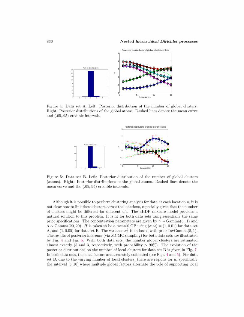
Figure 4: Data set A. Left: Posterior distribution of the number of global clusters.Right: Posterior distributions of the global atoms. Dashed lines denote the mean curveand (.05,.95) credible intervals.

1 2 3 4 50

50

100


0 5 10 15−2

−1

0

1

2


Locations u

Y

Figure 5: Data set B. Left: Posterior distribution of the number of global clusters(atoms). Right: Posterior distributions of the global atoms. Dashed lines denote themean curve and the (.05,.95) credible intervals.

Although it is possible to perform clustering analysis for data at each location u, it isnot clear how to link these clusters across the locations, especially given that the numberof clusters might be different for different u’s. The nHDP mixture model provides anatural solution to this problem. It is fit for both data sets using essentially the sameprior specifications. The concentration parameters are given by γ ∼ Gamma(5, .1) andα ∼ Gamma(20, 20). H is taken to be a mean-0 GP using (σ, ω) = (1, 0.01) for data setA, and (1, 0.05) for data set B. The variance σ2

ε is endowed with prior InvGamma(5, 1).The results of posterior inference (via MCMC sampling) for both data sets are illustratedby Fig. 4 and Fig. 5. With both data sets, the number global clusters are estimatedalmost exactly (5 and 3, respectively, with probability > 90%). The evolution of theposterior distributions on the number of local clusters for data set B is given in Fig. 7.In both data sets, the local factors are accurately estimated (see Figs. 4 and 5). For dataset B, due to the varying number of local clusters, there are regions for u, specificallythe interval [5, 10] where multiple global factors alternate the role of supporting local

X. Nguyen 837

3 4 5 6 70

10

20

30

40

50


0 5 10 15−2

−1

0

1

2


Locations u

Y

Figure 6: Effects of vague prior for H results in weak identifiability of global clusters,even as the local clusters are identified reasonably well.

1 2 3 4 50

20

40

60

80

100Num of local clusters at loc=1

1 2 3 4 50

20

40

60

80


1 2 3 4 50

20

40

60

80

100


1 2 3 4 50

20

40

60

80

100


1 2 3 4 50

20

40

60

80

100


1 2 3 4 50

20

40

60

80

100

120


1 2 3 4 50

20

40

60

80

100

120

140


1 2 3 4 50

20

40

60

80

100

120

140


Figure 7: Data set B: Posterior distribution of the number of local clusters associatingwith different group index (location) u.

clusters, resulting in wider credible bands.

In Section 3 we discussed the implications of prior specifications of the base measureH for the identifiability of global factors. We have performed a sensitivity analysis fordata set A, and found that the inference for global factors is robust when ω is set tobe in [.01, .1]. For ω = 0.5, for instance, which implies that φu are weakly dependentacross u’s, we are not able to identify the desired global factors (see Fig. 6), despite thefact that local factors are still estimated reasonably well.

The effects of prior specification for σε on the inference of global factors are somewhatsimilar to the hybrid DP model: a smaller σε encourages higher numbers of and lesssmooth global curves to expand the coverage of the function space (see Sec. 7.3 of [Nguyen and Gelfand (2010)]). Within our context, the prior for σε is relatively morerobust than that of ω as discussed above. The prior for concentration parameter γ isextremely robust while the priors for αu’s are somewhat less. We believe the reason forthis robustness is due to the modeling of the global factors in the second stage of the


0 5 10 15 20 25−3

−2

−1

0

1

2

3

4Progresterone hormone curves

Locations u

Y

Figure 8: Progeresterone hormone curves.

0 5 10 15 20 25−2

−1

0

1

2


Locations u

Y

0 5 10 15 20 25−1.5

−1

−0.5

0

0.5

1

1.5

2

2.5Posterior distributions of global cluster centers

Locations u

Y

Figure 9: Clustering results using the nHDP mixture model (Left), and the hybrid-DPof Petrone et al. (2009) (Right). Mean and credible intervals of global clusters (indashed lines) are compared to sample mean curves of the contraceptive group and nocontraceptive group in black solid with square markers.

nested hierarchy of DPs, and the inference about these factors has the effect of poolingdata from across the groups in the first stage. In practice, we take all αu’s to be equalto increase the robustness of the associated prior.

Progesterone hormone clustering. We turn to a clustering analysis of Progesteronehormone data. This data set records the natural logarithm of the progesterone metabo-lite, measured by urinary hormone assay, during a monthly cycle for 51 female subjects.Each cycle ranges from -8 to 15 (8 days pre-ovulation to 15 days post-ovulation). Weare interested in clustering the hormone levels per day, and assessing the evolution overtime. We are also interested in global clusters, i.e., identifying global hormone patternfor the entire monthly cycle and analyzing the effects on contraception on the cluster-ing patterns. See Fig. 8 for the illustration and [ Brumback and Rice (1998)] for moredetails on the data set.

X. Nguyen 839

10 20 30 40 50 60

10

20

30

40

50

60 0.75

0.8

0.85

0.9

0.95

1

10 20 30 40 50 60

10

20

30

40

50

600.3

0.4

0.5

0.6

0.7

0.8

0.9

1

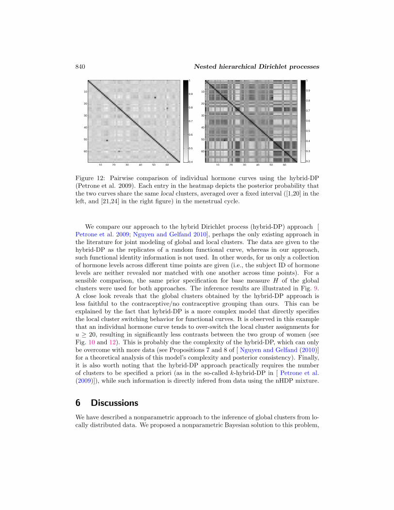
Figure 10: Pairwise comparison of individual hormone curves. Each entry in theheatmap depicts the posterior probability that the two curves share the same local

clusters, averaged over a fixed interval ([1,20] in the left, and [21,24] in the right figure)in the menstrual cycle.

1 2 30

10

20

30

40

50

60

70


1 2 30

10

20

30

40

50

60


1 2 30

10

20

30

40

50

60

70


1 2 30

20

40

60

80


1 2 30

20

40

60

80


Figure 11: The leftmost panel shows the posterior distribution of the number of globalclusters, while remaining panels show the the number of local clusters associating withgroup index u.

For prior specifications, we set γ ∼ Gamma(5, 0.1), and αu = 1 for all u. Letσε ∼ InvGamma(2, 1). For H , we set µ = 0, σ = 1 and ω = 0.05. It is found that thethere are 2 global clusters with probability close to 1. In addition, the mean estimate ofglobal clusters match very well with the sample means from the two groups of women,a group of those using contraceptives and a group that do not (see Fig. 9). Examiningthe variations of local clusters, there is a significant probability of having only one localcluster during the first 20 days. Between day 21 and 24 the number of local clusters is2 with probability close to 1.

To elaborate the effects of contraception on the hormone behavior (the last 17 femalesubjects are known to use contraception), a pairwise comparison analysis is performed.For every two hormone curves, we estimate the posterior probability that they share thesame local cluster on a given day, which is then averaged over days in a given interval. Itis found that the hormone levels among these women are almost indistinguishable in thefirst 20 days (with the clustering-sharing probabilities in the range of 75%), but in thelast 4 days, they are sharply separated into two distinct regimes (with the clustering-sharing probability between the two groups are dropped to 30%).


10 20 30 40 50 60

10

20

30

40

50

60

0.4

0.5

0.6

0.7

0.8

0.9

1

10 20 30 40 50 60

10

20

30

40

50

60

0.2

0.3

0.4

0.5

0.6

0.7

0.8

0.9

1

Figure 12: Pairwise comparison of individual hormone curves using the hybrid-DP(Petrone et al. 2009). Each entry in the heatmap depicts the posterior probability thatthe two curves share the same local clusters, averaged over a fixed interval ([1,20] in theleft, and [21,24] in the right figure) in the menstrual cycle.

We compare our approach to the hybrid Dirichlet process (hybrid-DP) approach [Petrone et al. 2009; Nguyen and Gelfand 2010], perhaps the only existing approach inthe literature for joint modeling of global and local clusters. The data are given to thehybrid-DP as the replicates of a random functional curve, whereas in our approach,such functional identity information is not used. In other words, for us only a collectionof hormone levels across different time points are given (i.e., the subject ID of hormonelevels are neither revealed nor matched with one another across time points). For asensible comparison, the same prior specification for base measure H of the globalclusters were used for both approaches. The inference results are illustrated in Fig. 9.A close look reveals that the global clusters obtained by the hybrid-DP approach isless faithful to the contraceptive/no contraceptive grouping than ours. This can beexplained by the fact that hybrid-DP is a more complex model that directly specifiesthe local cluster switching behavior for functional curves. It is observed in this examplethat an individual hormone curve tends to over-switch the local cluster assignments foru ≥ 20, resulting in significantly less contrasts between the two group of women (seeFig. 10 and 12). This is probably due the complexity of the hybrid-DP, which can onlybe overcome with more data (see Propositions 7 and 8 of [ Nguyen and Gelfand (2010)]for a theoretical analysis of this model’s complexity and posterior consistency). Finally,it is also worth noting that the hybrid-DP approach practically requires the numberof clusters to be specified a priori (as in the so-called k-hybrid-DP in [ Petrone et al.(2009)]), while such information is directly infered from data using the nHDP mixture.

6 Discussions

We have described a nonparametric approach to the inference of global clusters from lo-cally distributed data. We proposed a nonparametric Bayesian solution to this problem,

X. Nguyen 841

by introducing the nested Hierarchical Dirichlet process mixture model. This model hasthe virtue of simultaneous modeling of both local clusters and global clusters present inthe data. The global clusters are supported by a Dirichlet process, using a stochasticprocess as its base measure (centering distribution). The local clusters are supportedby the global clusters. Moreover, the local clusters are randomly selected using anotherhierarchy of Dirichlet processes. As a result, we obtain a collection of local clusterswhich are spatially varying, whose spatial dependency is regulated by an underlyingspatial or a graphical model. The canonical aspects of the nHDP (because of its use ofthe Dirichlet processes) suggest straightforward extensions to accomodate richer behav-iors using Poisson-Dirichlet processes (also known as the Pittman-Yor processes), wherethey have been found to be particularly suitable for certain applications, and where ouranalysis and inference methods can be easily adapted. It would also be interesting toconsider a multivariate version of the nHDP model. Finally, the manner in which globaland local clusters are combined in the nHDP mixture model is suggestive of ways ofdirect and simultaneous global and local clustering for various structured data types.

7 Appendix

7.1 Marginal approach to sampling

The Polya-urn characterization suggests a Gibbs sampling algorithm to obtain posteriordistributions of the local factors θui’s and the global factors ψt’s, by integrating out ran-dom measures Q and Gu’s. Rather than dealing with the θui’s and ψt directly, we shallsample index variables tui and kt instead, because θui’s and ψt’s can be reconstructedfrom the index variables and the φk’s. This representation is generally thought to makethe MCMC sampling more efficient. Thus, we construct a Markov chain on the space of{t,k}. Although the number of variables is in principle unbounded, only finitely manyare actually associated to data and represented explicitly.

A quantity that plays an important role in the computation of conditional proba-bilities in this approach is the conditional density of a selected collection of data items,given the remaining data. For a single observation i-th at location u, define the condi-tional probability of yui under a mixture component φuk, given t,k and all data itemsexcept yui:

f−yui

uk (yui) =

∫

F (yui|φuk)∏


∫∏


. (18)

Similary, for a collection of observations of all data yui such that tui = t for a chosen t,which we denote by vector yt, let f−yt

k (yt) be the conditional probability of yt underthe mixture component φk, given t,k and all data items except yt.

Sampling t. Exploiting the exchangeability of the tui’s within the group of observationsindexed by u, we treat tui as the last variable being sampled in the group. To obtain theconditional posterior for tui, we combine the conditional prior distribution for tui withthe likelihood of generating data yui. Specifically, the prior probability that tui takes on


a particular previously used value t is proportional to n−uiut , while the probability that

it takes on a new value tnew = mu + 1 is proportional to αu. The likelihood due to yuigiven tui = t for some previously used t is f−yui

uk (yui). Here, k = kt. The likelihood fortui = tnew is calculated by integrating out the possible values of ktnew :

p(yui|t−ui, tui = tnew,k,Data) =

K∑

k=1

qkq· + γ

f−yui

uk (yui) +γ

q· + γf−yui

uknew(yui), (19)

where f−yui

uknew(yui) =∫

F (yui|φu)Hu(φu)dφu is the prior density of yui. As a result, theconditional distribution of tui takes the form

p(tui = t|t−ui,k,Data) ∝

{

n−uiut f−yui

ukt(yui) if t previously used

αup(yui|t−ui, tui = tnew,k) if t = tnew.

(20)

If the sampled value of tui is tnew, we need to obtain a sample of ktnew by sampling fromEq. (19):

p(ktnew = k|t,k−tnew

,Data) ∝

{

qkf−yui

uk (yui) if k previously used,

γf−yui

uknew(yui) if k = knew.(21)

Sampling k. As with the local factors within each group, the global factors ψt’s arealso exchangeable. Thus we can treat ψt for a chosen t as the last variable sampled inthe collection of global factors. Note that changing index variable kt actually changesthe mixture component membership for relevant data items (across all groups u) thatare associated with ψt, the likelihood obtained by setting kt = k is given by f−yt

k (yt),where yt denotes the vector of all data yui such that tui = t. So, the conditionalprobability for kt is:

p(kt = k|t,k−t,Data) ∝

{

qkf−yt

k (yt) if k previously used,

γf−yt

knew(yt) if k = knew,(22)

where f−yt

knew(yt) =∫

∏

ui:tui=tF (yui|φu)H(φ)dφ.

Sampling of γ and α. We follow the method of auxiliary variables developed by [Escobar and West (1995)] and [ Teh et al. (2006)]. Endow γ with a Gamma(aγ , bγ)prior. At each sampling step, we draw η ∼ Beta(γ + 1, q·). Then the posterior of γ iscan be obtained as a gamma mixture, which can be expressed as πγGamma(aγ+K, bγ−log(η)) + (1− πγ)Gamma(aγ +K − 1, bγ − log(η)), where πγ = (aγ +K − 1)/(aγ +K −1 + q·(bγ − log(η))). The procedure is the same for each αu, with nu and mu playingthe role of q· and K, respectively. Alternatively, one can force all αu to be equal andendow it with a gamma prior, as in [ Teh et al. (2006)].

References

Aldous, D. (1985). “Exchangeability and related topics.” Ecole d’Ete de Probabilites

de Saint-Flour XIII-1983 , 1–198.

X. Nguyen 843

Antoniak, C. (1974). “Mixtures of Dirichlet Processes with Applications to BayesianNonparametric Problems.” Annals of Statistics, 2(6): 1152–1174.

Blackwell, D. and MacQueen, J. (1973). “Ferguson Distributions via Polya UrnSchemes.” Annals of Statistics, 1: 353355.

Brumback, B. and Rice, J. (1998). “Smoothing spline models for the analysis of nestedand crossed samples of curves.” J. Amer. Statist. Assoc., 93(443): 961–980.

Cifarelli, D. and Regazzini, E. (1978). “Nonparametric statistical problems under partialexchangeability: The role of associative means.” Technical report, Quaderni IstitutoMatematica Finanziaria dellUniversit‘a di Torino.

Cressie, N. (1993). Statistics for Spatial Data. Wiley, NY.

DeIorio, M., Mueller, P., Rosner, G., and MacEachern, S. (2004). “An ANOVA modelfor dependent random measures.” J. Amer. Statist. Assoc., 99: 205–215.

Duan, J., Guindani, M., and Gelfand, A. (2007). “Generalized spatial Dirichlet pro-cesses.” Biometrika, 94(4): 809–825.

Dunson, D. (2008). “Kernel local partition processes for functional data.” TechnicalReport 26, Department of Statistical Science, Duke University.

Dunson, D. and Park, J.-H. (2008). “Kernel stick-breaking processes.” Biometrika,95(2): 307–323.

Escobar, M. and West, M. (1995). “Bayesian Density Estimation and Inference UsingMixtures.” Journal of the American Statistical Association, 90: 577–588.

Ferguson, T. (1973). “A Bayesian analysis of some nonparametric problems.” Ann.

Statist., 1: 209–230.

Gelfand, A., Kottas, A., and MacEachern, S. (2005). “Bayesian nonparametric spatialmodeling with Dirichlet process mixing.” J. Amer. Statist. Assoc., 100: 1021–1035.

Griffin, J. and Steel, M. (2006). “Order-based dependent Dirichlet processes.” J. Amer.

Statist. Assoc., 101: 179–194.

Hjort, N., Holmes, C., Mueller, P., and (Eds.), S. W. (2010). Bayesian Nonparametrics:

Principles and Practice. Cambridge University Press.

Ishwaran, H. and James, L. (2001). “Gibbs sampling methods for stick-breaking priors.”J. Amer. Statist. Assoc., 96: 161–173.

Ishwaran, H. and Zarepour, M. (2002a). “Dirichlet prior sieves in finite normal mix-tures.” Statistica Sinica, 12: 941–963.

— (2002b). “Exact and Approximate Sum-Representations for the Dirichlet Process.”Canadian Journal of Statistics, 30: 269–283.


Jordan, M. (2004). “Graphical models.” Statistical Science, Special Issue on BayesianStatistics (19): 140–155.

Lauritzen, S. (1996). Graphical models. Oxford University Press.

Lo, A. (1984). “On a class of Bayesian nonparametric estimates I: Density estimates.”Annals of Statistics, 12(1): 351–357.

MacEachern, S. (1999). “Dependent Nonparametric Processes.” In Proceedings of the

Section on Bayesian Statistical Science, American Statistical Association.

MacEachern, S. and Mueller, P. (1998). “Estimating Mixture of Dirichlet Process Mod-els.” Journal of Computational and Graphical Statistics, 7: 223–238.

Mueller, P., Quintana, F., and Rosner, G. (2004). “A Method for Combining InferenceAcross Related Nonparametric Bayesian Models.” Journal of the Royal Statistical

Society , 66: 735749.

Muliere, P. and Petrone, S. (1993). “A Bayesian Predictive Approach to SequentialSearch for an Optimal Dose: Parametric and Nonparametric Models.” Journal of the

Italian Statistical Society , 2: 349364.

Muliere, P. and Secchi, P. (1995). “A note on a proper Bayesian bootstrap.” TechnicalReport 18, Dipartimento di Economia Politica e Metodi Quantitativi, Universita degliSudi di Pavia.

Neal, R. (1992). “Bayesian Mixture Modeling.” In Proceedings of the Workshop on

Maximum Entropy and Bayesian Methods of Statistical Analysis, volume 11, 197–211.

Nguyen, X. and Gelfand, A. (2010). “The Dirichlet labeling process for clusteringfunctional data.” Statistica Sinica, to appear.

Petrone, S., Guidani, M., and Gelfand, A. (2009). “Hybrid Dirichlet processes forfunctional data.” Journal of the Royal Statistical Society B, 71(4): 755–782.

Pittman, J. (2002). “Poisson-Dirichlet and GEM invariant distributions for split-and-merge transformations of an interval partition.” Combinatorics, Probability and Com-

puting , 11: 501–514.

Rabiner, L. (1989). “A Tutorial on Hidden Markov Models and Selected Applicationsin Speech Recognition.” Proceedings of the IEEE, 77: 257–285.

Rodriguez, A. and Dunson, D. (2009). “Nonparametric Bayesian models through probitstick-breaking processes.” Technical report, University of California, Santa Cruz.

Rodriguez, A., Dunson, D., and Gelfand, A. (2010). “Latent stick-breaking processes.”J. Amer. Statist. Assoc., 105(490): 647–659.

Schwartz, L. (1965). “On Bayes procedures.” Z. Wahr. Verw. Gebiete, 4: 10–26.

X. Nguyen 845

Sethuraman, J. (1994). “A constructive definition of Dirichlet priors.” Statistica Sinica,4: 639–650.

Teh, Y., Jordan, M., Beal, M., and Blei, D. (2006). “Hierarchical Dirichlet processes.”J. Amer. Statist. Assoc., 101: 1566–1581.

Teh, Y. W. and Jordan, M. I. (2010). “Hierarchical Bayesian nonparametric modelswith applications.” Bayesian Nonparametrics: Principles and Practice, In N. Hjort,C. Holmes, P. Mueller, and S. Walker (Eds.).

Wainwright, M. J. and Jordan, M. I. (2008). “Graphical models, exponential families,and variational inference.” Foundations and Trends in Machine Learning , 1: 1–305.

Acknowledgments

This work was partially supported by NSF-CDI grant No. 0940671. The author wishes to thank

the referees and the Associate Editor for valuable comments that help improve the presentation

of this work.


Documents

Inference of global clusters from locally distributed datadept.stat.lsa.umich.edu/~xuanlong/Papers/nguyen-ba-10.pdf · Bayesian Analysis (2010) 5, Number 4, pp. 817–846 Inference