Embed Size (px)
Citation preview

PREPRINT
Infectious Disease Modelling
Michael HohleDepartment of Mathematics, Stockholm University, Sweden
16 March 2015
This is an author-created preprint of a book chapter to appear in the Hand-book on Spatial Epidemiology edited by Andrew Lawson, Sudipto Banerjee, RobertHaining and Lola Ugarte, CRC Press. The final version of this text is tobe found in this book – once available the ISBN number of the book will begiven. The preprint is available as http://www.math.su.se/~hoehle/pubs/Hoehle_SpaMethInfEpiModelling2015.pdf
1 Introduction
Infectious diseases impose a critical challenge to human, animal and plant health. Emergingand re-emerging pathogens – like SARS, influenza, hemorrhagic fever among humans, or footand mouth disease and classical swine fever among animals – hit the news coverage withregular certainty. Zoonoses and host transmitted diseases underline how tight the connectionis between human and animal diseases. While plant epidemics receive less immediate atten-tion, they can severely impact crop yield or wipe out entire species. Unifying for the aboveepidemics is that they all represent realization of temporal processes. Why does the spatialdimension then matter for the modelling of epidemics? It depends very much on the aims ofthe analysis: Many relevant questions can be adequately answered by models considering thepopulation as being homogeneous. However, in other situations heterogeneity is important,e.g., induced by age or spatial structure of the population. Spatially varying demographicand environmental factors could influence the disease transmission. Furthermore, having aspatial resolution allows the model to express spatial heterogeneity in the manifestation of thedisease over time. This becomes particularly important when investigating the probability offade-out or short-term predicting the location of new cases. This kind of analysis representsan important mathematical contribution aimed at understanding the dynamics of diseasetransmission and predicting the course of epidemics in order to, for example, assess controlmeasures or determine the source of an epidemic. This chapter is about the spatio-temporalanalysis of epidemic processes.
2 The Role of Space in Infectious Disease Epidemiology
The focus in this chapter will be on communicable microparasite infections (typically viralor bacterial diseases) among humans – though the application of mathematical modelling isequally immediate in animal (Dohoo et al., 2010) and plant epidemics (Madden et al., 2007).
Following Giesecke (2002), epidemiology is about ’the study of diseases and their determi-nants in populations’. The concepts of incidence and prevalence, known from chronic disease
1

PREPRINT
2 The Role of Space in Infectious Disease Epidemiology
epidemiology, also apply to infectious disease epidemiology. However, contrary to chronicdisease modelling it is important to realize that in infectious disease epidemiology each caseis also a risk factor and that not everyone is necessarily susceptible to a disease (e.g. immu-nity due to previous infections or vaccination). As a consequence, the study of infectiousdiseases is very much concerned with the study of interacting populations. Still, as treated infor example Becker (1989) or Hens et al. (2012), the principal of regression by linear models(LMs), generalized linear models (GLMs) or survival models applies to a variety of problemsin infectious disease epidemiology. Hence, spatial extensions of such regression models, e.g.structured additive regression models (Fahrmeir and Kneib, 2011), also immediately applyto the context of infectious disease epidemiology. Examples are the use of spatially enhancedecological Poisson regression models with CAR random effects to investigate the influence ofsocio-economic factors on the incidence of specific infectious diseases (Wilking et al., 2012)or the assessment of mumps outbreak risk based on serological data by using generalizedadditive models (GAMs) with 2D splines adjusting for location of individuals (Abrams et al.,2014). Another application of classical methods from spatial epidemiology is the use of spatialpoint process models for investigating putative sources for a foodborne outbreak (Diggle andRowlingson, 1994).
In this chapter we will, however, restrict the focus to the use of spatio-temporal trans-mission models, that is dynamic models for the person-to-person spread of a disease in awell defined population. The use of such models has become increasingly popular in theepidemiological literature in order to assess risk of emerging pathogens or evaluate controlmeasures. Even spatial aspects of such evaluations are now feasible due to the fact that databecome spatially more refined and computer power allows for more complex models to beinvestigated. The modelling of measles and influenza are two examples where the impact ofspace has been especially thoroughly investigated (Grenfell et al., 1995, 2001; Viboud et al.,2006; Eggo et al., 2011; Gog et al., 2014). As an illustration, we will look in detail at thespatio-temporal modelling of biweekly measles counts in 60 towns and cities in England andthe UK, 1944-1966. Figure 1 shows the locations of the 60 cities, including both very largeand very small cities, and forming a subset of the data for 954 communities used in Xia et al.(2004). An illustration of the the time series for the three largest and three smallest cities inthe data set can be found as part of Fig. 5. The aim of such an analysis is to quantify theeffect of demographics and seasonality on the dynamics, but also to investigate the role ofspatial spread on extinction and re-introduction.
In spatial analyses of this kind the movement of populations plays an important role. Froma historic perspective especially mobility has undergone dramatic changes within the last 200years – for instance Cliff and Haggett (2004) talk about this as the ’collapse of geographicalspace’: The time for travelling long distances has reduced immensely, which has resultedin populations mixing at increasingly higher rates. Whilst there has been an abundanceof papers and animations illustrating global spread of emerging diseases, e.g. due to airlinetravelling, the core transmission of many ’neglected’ diseases still occurs at short-range: inthe household, in the kindergarten, at work. The role of space in transmission models isto be studied within this dissonance between long-distance and short-distance spread. Anumber of chapters and articles have already surveyed this field, e.g. Isham (2004), Deardonet al. (2015), Riley et al. (2014) and Held and Paul (2013). The emphasis in the presentchapter is on metapopulation models and their likelihood based inference. It is structuredas follows: Section 3 consists of a primer on continuous-time and discrete time epidemicmodelling – first for a homogeneous population and then for spatially coupled populations.Section 4 then illustrates the application of discrete-time versions of such models to the 60
2

PREPRINT−200 0 200 400 600 800 1000
010
020
030
040
050
060
0
●
●
●
●●●
●
●
●
●
●
●
●
●
●
●
●
●
●
● ●
●
●
●
●
●
●
●●
●
●
●
●●
●
●
●
●
●
●
●
● ●
●
●
●
● ●
●
●
●
●
●
●
●
●●
●
●
●
●
●
Population
104
105
106
100km
Figure 1: Location of the 60 cities in England and Wales (OSGB36 reference system) usedin the measles modelling. The area of each circle is proportional to the city’s population andthe connecting lines indicate immediate neighbourhood (distance ≤50 km).
cities measles data. A discussion in Section 5 ends the chapter.
3 Epidemic Modelling
Mathematical modeling of infectious diseases has become a key tool in order to understand,predict and control the spread of infections. The fundamental difference to chronic diseaseepidemiology is that the temporal aspect is paramount. The aim of epidemic modelling isthus to model the spread of a disease in a population made up of a (possibly large) integernumber of individuals. To simplify the description of this population, it is common to usea compartmental approach to modelling – for instance in its simplest form the population isdivided into classes of susceptible, infective and recovered individuals. Disease dynamics canthen be characterized by a mathematical description of each individual’s transitions betweencompartments, subject to the state of the remaining individuals.
3.1 Continuous time modelling
A number of books, e.g. Anderson and May (1991), Diekmann and Heesterbeek (2000),Keeling and Rohani (2008), give an introduction to epidemic modelling using primarily de-terministic models based on ordinary differential equations (ODEs) in the setting of thesusceptible-infective-recovered (SIR) model and its extensions. Let S(t), I(t) and R(t) de-note the number at time t of susceptible, infective and recovered individuals, respectively.Then the dynamics in the basic deterministic SIR model in a population of fixed size can beexpressed as in the seminal work by Kermack and McKendrick (1927):
dS(t)
dt= − β
NS(t)I(t),
dI(t)
dt=
β
NS(t)I(t)− γI(t),
dR(t)
dt= γI(t),
where the parameter β > 0 is the transmission rate and γ > 0 describes the removal rate.The initial condition is given by S(0), I(0), which are known integers, and R(0) = 0. In
3

PREPRINT
3 Epidemic Modelling
a population of fixed size N = S(0) + I(0) the expression for dR(t)/dt in the above ODEsystem is redundant because R(t) is implicitly given as N − S(t)− I(t).
ODE modelling implies an approximation of the integer sized population using continuousnumbers and that the stochastic behaviour of an epidemic is sacrificed by looking at a deter-ministic average behavior. If the population under study is large enough, such approximationsare reasonably valid to obtain a biological understanding. In small populations, however,stochasticity plays an important role for extinction, which cannot be ignored. Stochastic epi-demic modelling is described e.g. in Bailey (1975), Becker (1989), Daley and Gani (1999) andAndersson and Britton (2000), who all rely heavily on the theory of stochastic processes. Inits simplest form, the basic discrete-state stochastic SIR model can be described as a generalbirth and death process, where the event rates for infection and removal are given as follows:
Event Rate
(S(t), I(t))→ (S(t)− 1, I(t) + 1) βN S(t)I(t)
(S(t), I(t))→ (S(t), I(t)− 1) γI(t)
Again, the development of R(t) is implicitly given, because a fixed population of size S(0) +I(0) is assumed. Notice also how the integer size of the population is now taken into account:Once I(t) = 0, the epidemic ceases. From a point process viewpoint the above specificationcorresponds to an assumption of piecewise constant conditional intensities for the processof infection, while the length of the infective period is given by independent and identicallydistributed exponential random variables. An important point is that the deterministic SIRmodel is not just modelling the expectation of the stochastic SIR model. As an illustration,Renshaw (1991, Chapter 10) shows, based on calculations in Bailey (1950), how the expectednumber of susceptibles µ(t) = E(S(t)) in the stochastic SI model differs from the solution ofS(t) in the deterministic SI model. Figure 2 shows the result for a population with S(0) = 10,I(0) = 1, β = 11 and γ = 0. One notices the differences between the deterministic andstochastic model.
Finding an analytic expression for µ(t) or – even better – the probability mass function(PMF) of S(t) at a specific time point t is less easy already for the SIR model and intractablefor most models. Instead, a numerical approach is to formulate a first order differential-difference equation describing the time evolution of P ((S(t), I(t)) = (x, y)) for each possible(x, y). Such an approach is known as a master equation approach and corresponds to a discretestate continuous time Markov jump process with the solution of the master equation obeyingthe Chapman-Kolmogorov equation. These ODE equations are then solved numerically. Forlarge populations the problem can, however, become intractable to solve even numerically.For further details on such stochastic population modelling see, e.g., Renshaw (1991). Analternative to the above is to resort to Monte Carlo simulation of the stochastic epidemicprocess – a method which has become increasingly popular even for inferential purposes. Forthe basic SIR model one needs to simulate a discrete-state continuous-time stochastic processwith piecewise constant conditional intensity functions (CIFs). Several algorithms exist fordoing this, see e.g. Wilkinson (2006) for an overview, of which the algorithm by Gillespie(1977) is the best known. As an example, Fig. 2 shows 10 realizations of the previousSI model and the resulting empirical probability distribution of S(t) computed from 1000simulations. Besides simplicity Monte Carlo simulations have the additional advantage ofbeing very flexible. For example, it is easy to use the samples to compute pointwise 95%prediction intervals for S(t) or to compute the final number of infected.
A further important difference between deterministic and stochastic modelling is the in-terpretation of the basic reproduction number R0, which describes the reproductive potential
4

PREPRINT
3.2 A Spatial Extension: The Metapopulation Model
0.0 0.2 0.4 0.6 0.8 1.0
02
46
810
t
S(t
)
µ(t)Sdet(t)
0.0 0.2 0.4 0.6 0.8 1.0
02
46
810
t
S(t
)
µ(t)empirical meanSdet(t)
0
250
500
750
1000Scale
Figure 2: (left) S(t) for 10 realizations of the SI model with parameters as described in thetext. Also shown is E(S(t)) in the stochastic model and the solution S(t) in the determin-istic model. (right) Histograms of the S(t) distribution based on 1000 realizations. The 23histograms are computed for a grid between time 0.0 and 1.1 with a step size of 0.05. Alsoshown are the analytic mean µ(t) together with the 23 empirical means.
of an infectious disease and which is defined as the average number of secondary cases directlycaused by an infectious case in an entirely susceptible population. In deterministic modelsa major outbreak can only occur if R0 > 1. In stochastic models, if R0 > 1, then an majoroutbreak will occur with a certain probability determined by the model parameters. See, e.g.,Andersson and Britton (2000) or Britton (2010) for further details.
Other variations of the basic SI and SIR model could be, for example, the SI-Susceptible,SIR-Susceptible or S-Exposed-IR model. Further extensions consist of reflecting the protec-tion due to maternal antibodies or vaccination by respective compartments in the models.Finally, the rates can be additionally modified to, e.g., reflect the import of infected from out-side the population or demographics such as birth and death of individuals. See, e.g. Keelingand Rohani (2008, Chapter 2) for additional details.
3.2 A Spatial Extension: The Metapopulation Model
If interest is in enhancing the homogeneous SIR model with heterogeneity due to spatialaspects, one common modelling approach is to divide the overall population into a number ofsubpopulations – a so called metapopulation model (Keeling et al., 2004, Chapter 17). Here,one assumes that within each subpopulation the mixing is homogeneous whereas couplingbetween the subpopulations occurs by letting the force of infection contain contributions ofthe infectious from the other populations as well. Considering a total of K subpopulationsthe deterministic metapopulation SIR model looks as follows (Keeling and Rohani, 2008,
5

PREPRINT
3 Epidemic Modelling
Chapter 7.2):
dSk(t)
dt= − βk
NkSk(t)
(K∑l=1
wklIl(t)
), k = 1, . . . ,K,
dIk(t)
dt=
βkNk
Sk(t)
(K∑l=1
wklIl(t)
)− γIk(t),
where the weights wkl quantify the impact of one infectious from population l on populationk. Typically, these weights are scaled such that wkk = 1, k = 1, . . . ,K. Consequently, fora susceptible in k, wkl represents the influence of an infectious in unit l relative to one inthe same unit as the susceptible. The appropriate choice of weights depends on the modelleddisease, its mode of transmission and the questions to be answered. They can even be subjectto parametric modelling: For plant or animal diseases dispersal could for example be due toairborne spread which makes distance kernels such as exponential wkl ∝ exp(−ρdistkl) orpower law wkl ∝ dist−ρkl convenient choices. Here, distkl denotes the geographic distancebetween the population k and l. When restricting attention to directly transmitted humandiseases the focus is instead on the movement of infectious individuals from population l topopulation k – not necessarily due to a permanent relocation of individuals, but more dueto temporarily movement. This could, for instance in the case of seasonal influenza, be thecommuting of individuals or in the case of emerging epidemics (e.g. SARS, swine influenza)due to long-distance airplane travelling. If commuter or airline data are available these can beused to determine the weights. Movement exhibits a strong age-dependence, though, whichcan make it difficult to extract the relevant information from such sources for childhooddiseases. As a consequence, one might use distance based kernels as a proxy for mobility– possibly augmented by population sizes as in the gravity model (Erlander and Stewart,1990; Xia et al., 2004). If interest is in short-term prediction of an emerging pathogen, long-distance travelling is an important concept to capture. However, the main bulk of infectionsfor an established disease typically happens at a much smaller geographical scale as shown,for example, in recent re-analyses of the 1918 pandemic influenza (Eggo et al., 2011) and the2009 swine influenza outbreak (Gog et al., 2014).
In analogy to the above deterministic metapopulation model, the system of rates of thecontinuous time stochastic SIR model can be modified accordingly to obtain a stochasticmetapopulation model with unit specific (conditional) intensity function for infection events
λk(t) =βkNk
Sk(t)
(K∑l=1
wklIl(t)
), (1)
while the unit specific intensity function for recovery events is now γIk(t) (assuming expo-nentially distributed infectious periods). One important insight is that the difference betweendeterministic and stochastic metapopulation models is increased as subpopulations becomesmaller. Studying the extinction and re-introduction of disease in such metapopulations ishence preferably conducted using stochastic metapopulation models, see e.g. Bjørnstad andGrenfell (2008). Two variants of the stochastic metapopulation model are of additional inter-est: The first variant is the so called Levins-type metapopulation model (Keeling and Rohani,2008, Section 7.2.4), where one for each k is only interested in the probability of Ik(t) > 0as a function of time. Such models have been used to study the arrival of the first diseasecases in a city during a pandemic (Eggo et al., 2011; Gog et al., 2014). The second variant
6

PREPRINT
3.3 Fitting SIR Models to Data
is the individual model, i.e. when the number of considered subpopulations is equal to thepopulation size K = N .
Both cases are instances of multivariate counting processes which can be consistently han-dled in the SIR-S framework using a so called two-component SIRS model, which additionallyallows for immigration of disease case from external sources. This is particularly useful if thedata contains multiple outbreaks. Following Hohle (2009) let Nk(t), k = 1, . . . ,K, denote thecounting process, which for unit k counts the number of changes from state susceptible tostate infectious. The conditional intensity function given the history of all K processes upto, but not including, t is then given as:
λk(t) = exp(h0(t) + zk(t)
Tβ)
+∑j∈I(t)
{w(distkj) + vkj(t)
Tαe
}(2)
= Yk(t) ·[exp(h0(t)) exp
(zk(t)
Tβ)
+ xk(t)Tα],
where Yk(t) is an indicator if unit k is susceptible, i.e. Yk(t) = 1k∈S(t)), while S(t) and I(t)now denotes the index set of all susceptibles and infectious, respectively. Furthermore, w(·)denotes a distance weighting kernel parametrised as a spline function while zk(t) and vkj(t)denote possibly time varying covariates affecting the introduction of new cases in the endemicand epidemic components, respectively, and xk(t) denotes the combination of linear splineterms and epidemic covariates. Finally, h0(t) is the base-line rate of the endemic component.If import of new cases from external sources is not relevant the first component in the abovecan be left out (i.e. set to zero).
3.3 Fitting SIR Models to Data
From a statistician’s point of view, parameter inference in epidemic models appears to re-ceive only marginal attention in the medical literature. One reason might be that little orno data are available and hence parameters are ’guesstimated’ from literature studies or ex-pert knowledge. Another reason is that inference often boils down to extracting informationabout parameter values from a single realization of the stochastic epidemic process. Fordeterministic models, estimation might also appear less of a statistical issue. Finally, esti-mation is complicated by the epidemic process only being partially observable: The numberof susceptibles to begin with as well as the time point of infection of each case with mightbe unknown. As a consequence, parameter estimation in ODE based SIR models has, typ-ically, been done using least square type estimation based on observable quantities. Onlyrecently, the models have been extended to non-Gaussian observational components enablingcount-data likelihood based statistical inference, see e.g. Pitzer et al. (2009),
E(Yt,k) =
∫ t+1
t
{−dSk(u;θ)
dt
}du.
where Yt,k is the observed number of new infections within time interval t, which is assumedto follow a count data PMF f such as the Poisson or negative binomial distribution with ex-pectation E(Yt,k). This setup allows the estimation of the model parameters ψ in a likelihood
framework by the loglikelihood function l(ψ) =∑T
t=1
∑Kk=1 log f(yt,k;ψ), when assuming
observations are independent given the model. However, a residual analysis often shows re-maining auto-correlation, which means any quantification of estimation uncertainty basedon asymptotic theory using the Hessian of the loglikelihood tends to be overly optimistic.As a consequence, the confidence intervals might be too narrow. A novel two-step approach
7

PREPRINT
3 Epidemic Modelling
to improve on this shortcoming within the above framework is treated in Weidemann et al.(2014).
An advantage of stochastic continuous-time SIR modelling is that it allows for a quan-tification of the uncertainty of the estimates, even though the estimate is based on a singleprocess realization. The work of Becker (1989) and the second part of Andersson and Britton(2000) are some of the few books dedicated to this task. If the epidemic process (S(t), I(t))′
is completely observed over the interval (0, T ], where T is the entire duration of the epidemic,the resulting data of the epidemic are given as {(ti, yi, ki), i = 1, . . . , n}, where n is the num-ber of infections in the population during the epidemic, ti denotes the time of infection ofindividual i, yi is the length of the individuals’ infectious period and ki ∈ {1, . . . ,K} is theunit it belongs to. Further assuming that the PDF of the infectious period is exponentialfI→R(y) = γ exp(−γy) we obtain the loglikelihood for the parameter vector ψ = (β, γ)′ as
l(ψ) =
n∑i=1
log fI→R(yi) +
n∑i=1
log λki(ti)−∫ T
0
K∑k=1
λk(u)du, (3)
where λk(ti) is defined as in (1) and evaluated at the time just prior to ti. Note that in (3) theCIFs have to be integrated over time, however, for the simple SIR model the CIF is a piecewiseconstant function between events and hence integration is tractable. Hohle (2009) developsthese likelihood equations further using counting process notation for the two-componentSIR model (2), whereas Lawson and Leimich (2000), Diggle (2006) and Scheel et al. (2007)contain accounts and examples of a partial-likelihood approach for spatial SIR type modelinference including covariates.
In applications the times of infection ti of infected individuals would typically be unknown.One way to make inference tractable is to assume that the duration of the infectious periodis a constant, say, µI→R (known or to be estimated). Furthermore, the initial number ofsusceptibles might also be unknown and might require estimation. See Becker (1989) fordetails, which also covers a discrete-time approximation covered in the next section. Morerecently, Gibson and Renshaw (1998), O’Neill and Roberts (1999), O’Neill and Becker (2001),Neal and Roberts (2004) and Hohle et al. (2005) use a Bayesian data augmentation approachusing Markov Chain Monte Carlo to impute the missing infection times while simultaneouslyperforming Bayesian parameter inference for the S(E)IR and metapopulation S(E)IR model.Model diagnostics can in the likelihood context be performed using a graphical assessmentof residuals and forward simulation (Hohle, 2009); for the Bayesian models one can useadditional posterior predictive checks and latent residuals (Lau et al., 2014).
3.4 Discrete time models
Up to now, focus has been on continuous time epidemic modeling. However, data are usuallyonly available at much coarser time scales: weekly or daily reporting is usual in public healthsurveillance. If individual data is available, this observational situation can be handled byconsidering the observed event times as being for the event times interval censored. However,when looking at large populations or routinely collected data, data is typically providedin aggregated form without access to the individual data. It is thus necessary to consideralternative ways of casting the continuous time stochastic SIR approach into a discrete timeframework. Time series analysis is one such approach, providing a synthesis between complexstochastic modeling and available data.
In order to derive such a model, we consider a sufficiently small time interval [t, t + δt).We could then – as an approximation – assume constant conditional intensity functions of our
8

PREPRINT
3.5 Time Series SIR model
SIR model in [t, t+δt). By definition, let these intensities be equal to the intensities at the lefttime point of the interval, i.e. at time t. This implies that all individuals are independent forthe duration of the interval. Looking at one susceptible individual, its probability of escapinginfection during [t, t+ δt) is then equal to exp(−βI(t) · δt). Denoting by C[t,t+δt) the numberof newly infected and by D[t,t+δt) the number of recoveries in the interval [t, t+ δt), we obtain
C[t,t+δt) ∼ Bin(S(t), 1− exp(−βI(t) · δt)
), (4)
D[t,t+δt) ∼ Bin(I(t), 1− exp(−γ · δt)
). (5)
The state at time t+δt is then given by S(t+δt) = S(t)−C[t,t+δt), I(t+δt) = I(t)+C[t,t+δt)−D[t,t+δt). Now changing notation to discrete time with discrete time subscript t denoting thetime t+ δt and subscript t− 1 the time t we write:
St = St−1 − Ct, It = It−1 + Ct −Dt, (6)
for t = 1, 2, . . . and with S0 = S(0), I0 = I(0). Consequently, the discrete quantities Ct,Dt, etc. now replace the continuous ones in (4) and (5). Such models are known as chainbinomial models (Becker, 1989), if one assumes that Dt = It, i.e. the time scale is chosensuch that all infective individuals recover after one time step. In such models one time stepcan be seen as one generation time (Daley and Gani, 1999, Chapter 4). For large St and Itthe binomial distributions can be further approximated by Poisson distributions: by a firstorder Taylor expansion of the 1− exp(−x) terms one obtains
Ct ∼ Po(βSt−1It−1 · δt
), (7)
Dt ∼ Po(γIt−1 · δt
). (8)
Note that these approximations no longer ensure that Ct ≤ St−1 and Dt ≤ It−1. If thisis a practical concern, one can instead use right truncated Poisson distributions fulfillingthe conditions. Altogether, we have transformed the continuous time stochastic model into adiscrete time model. If (St, It)
′ is known at each point in time t = 1, . . . , T , estimates for β andγ can be found using maximum likelihood approaches based on (7)-(8). For example, Becker(1989) shows how the above equations can be used to fit a homogeneous SIR model to datausing generalized linear model (GLM) software: (8) can be represented as a log-link PoissonGLM with offset log(St−1It−1δt) and intercept log(β) or an identity link GLM with covariateSt−1It−1δt and no intercept. For the stochastic metapopulation SIR model with knownweights the idea can similarly be extended by jointly modelling Ct,k and Dt,k, 1 ≤ t ≤ T ,1 ≤ k ≤ K by an appropriate Poisson GLM with either log-link or identity link with offset,intercept and potential covariates derived from (1). Furthermore, Klinkenberg et al. (2002)uses the above equations to fit a spatial grid SIR model using numerical maximization of thebinomial likelihood.
3.5 Time Series SIR model
The model given by (7)-(8) corresponds to a simple version of the time series SIR model (TSIRmodel) initially proposed in Finkenstadt and Grenfell (2000) and since extended (Finkenstadtet al., 2002; Bjørnstad et al., 2002). For the TSIR model it is assumed that Dt = It, i.e. as ina chain binomial model, and δt = 1. As an example, one time unit corresponds to a biweeklyscale when modelling measles. In addition, the TSIR model contains additional flexibility
9
PREPRINT
3 Epidemic Modelling
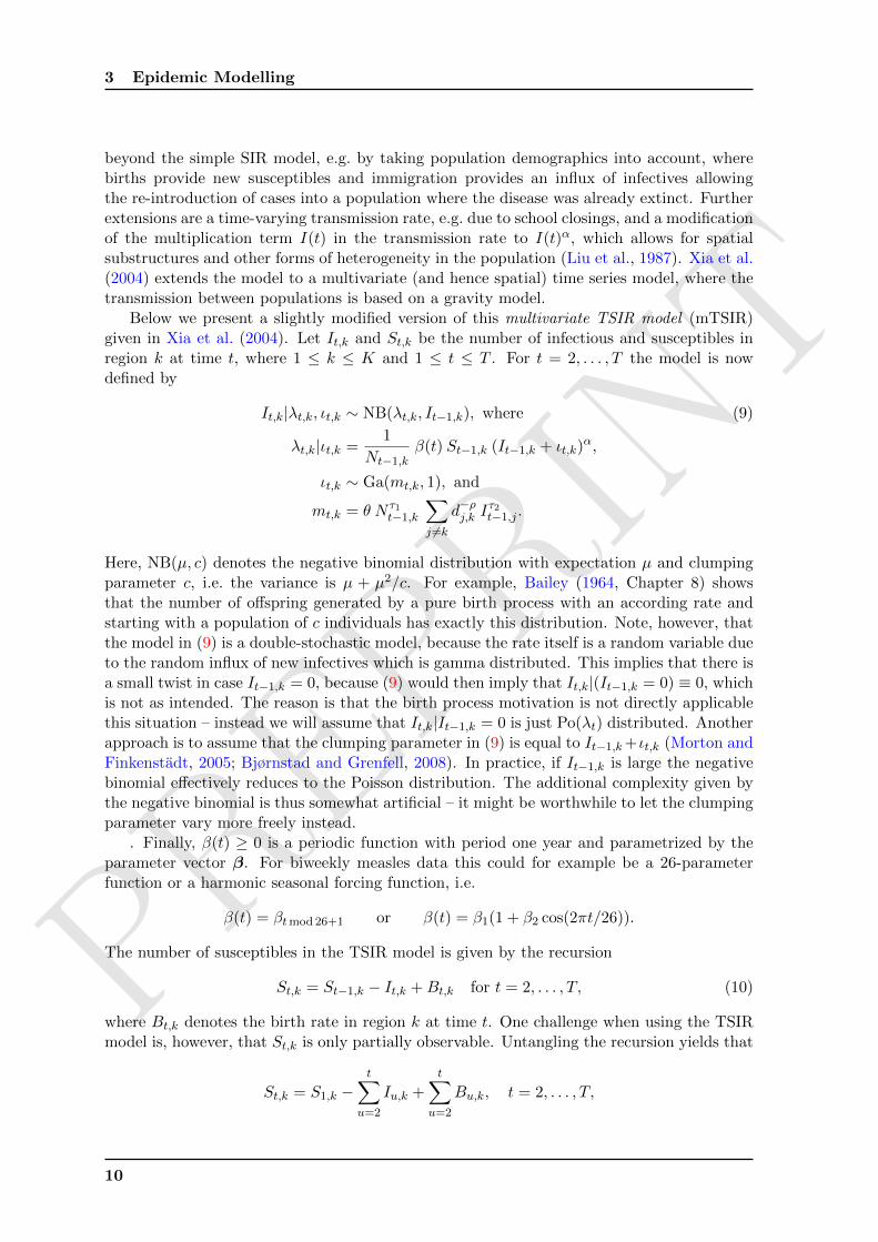
beyond the simple SIR model, e.g. by taking population demographics into account, wherebirths provide new susceptibles and immigration provides an influx of infectives allowingthe re-introduction of cases into a population where the disease was already extinct. Furtherextensions are a time-varying transmission rate, e.g. due to school closings, and a modificationof the multiplication term I(t) in the transmission rate to I(t)α, which allows for spatialsubstructures and other forms of heterogeneity in the population (Liu et al., 1987). Xia et al.(2004) extends the model to a multivariate (and hence spatial) time series model, where thetransmission between populations is based on a gravity model.
Below we present a slightly modified version of this multivariate TSIR model (mTSIR)given in Xia et al. (2004). Let It,k and St,k be the number of infectious and susceptibles inregion k at time t, where 1 ≤ k ≤ K and 1 ≤ t ≤ T . For t = 2, . . . , T the model is nowdefined by
It,k|λt,k, ιt,k ∼ NB(λt,k, It−1,k), where (9)
λt,k|ιt,k =1
Nt−1,kβ(t) St−1,k (It−1,k + ιt,k)
α,
ιt,k ∼ Ga(mt,k, 1), and
mt,k = θ N τ1t−1,k
∑j 6=k
d−ρj,k Iτ2t−1,j .
Here, NB(µ, c) denotes the negative binomial distribution with expectation µ and clumpingparameter c, i.e. the variance is µ + µ2/c. For example, Bailey (1964, Chapter 8) showsthat the number of offspring generated by a pure birth process with an according rate andstarting with a population of c individuals has exactly this distribution. Note, however, thatthe model in (9) is a double-stochastic model, because the rate itself is a random variable dueto the random influx of new infectives which is gamma distributed. This implies that there isa small twist in case It−1,k = 0, because (9) would then imply that It,k|(It−1,k = 0) ≡ 0, whichis not as intended. The reason is that the birth process motivation is not directly applicablethis situation – instead we will assume that It,k|It−1,k = 0 is just Po(λt) distributed. Anotherapproach is to assume that the clumping parameter in (9) is equal to It−1,k+ιt,k (Morton andFinkenstadt, 2005; Bjørnstad and Grenfell, 2008). In practice, if It−1,k is large the negativebinomial effectively reduces to the Poisson distribution. The additional complexity given bythe negative binomial is thus somewhat artificial – it might be worthwhile to let the clumpingparameter vary more freely instead.
. Finally, β(t) ≥ 0 is a periodic function with period one year and parametrized by theparameter vector β. For biweekly measles data this could for example be a 26-parameterfunction or a harmonic seasonal forcing function, i.e.
β(t) = βtmod 26+1 or β(t) = β1(1 + β2 cos(2πt/26)).
The number of susceptibles in the TSIR model is given by the recursion
St,k = St−1,k − It,k +Bt,k for t = 2, . . . , T, (10)
where Bt,k denotes the birth rate in region k at time t. One challenge when using the TSIRmodel is, however, that St,k is only partially observable. Untangling the recursion yields that
St,k = S1,k −t∑
u=2
Iu,k +t∑
u=2
Bu,k, t = 2, . . . , T,
10

PREPRINT
3.6 Fitting the mTSIR Model to Data
where S1,k is usually unknown but needs to be such that 0 < St,k ≤ Nt,k − It,k for allt = 2, . . . , T . As a consequence, either all unknown S1,k’s need to enter the analysis as Kadditional parameters or one has just a single extra parameter κ together with the coarseassumption that S1,k = κN1,k. An alternative is to use a pre-processing step to determine it:Conditional on S1,k and the observed It,k one can compute the resulting St,k’s. Inspired bythe univariate procedure in Finkenstadt et al. (2002) one then considers ιt,k within the unitto be a time series varying around its mean and uses a Taylor expansions up to order threeto derive
log It,k = log βt + α log(It−1,k) + c1I−1t−1,k + c2I
−2t−1,k + c3I
−3t−1,k + logSt,k + εt,k, (11)
where the εt,k’s are zero-mean random variables. Altogether, conditionally on S1,k expression(11) represents a linear regression model which can be fitted using maximum likelihood. Theresulting profile loglikelihood in S1,k can then be optimized for each unit separately.
As already mentioned, one problem with the above model formulation, is that the updategiven in (9) does not ensure that It,k ≤ St−1,k+Bt−1,k. In other words St,k ≥ 0 is not explicitlyensured by the model. When fitting the model to data this is unproblematic, because theSt,k’s are computed by a separate pre-processing step. However, when simulating from themodel and hence computing St,k in each step from (10) it becomes clear that these can becomenegative if It,k is large enough. To ensure validity of the model we thus right-truncate theNB(λt,k, It−1,k) at St−1,k.
3.6 Fitting the mTSIR Model to Data
In the work of Xia et al. (2004) a heuristic optimization criterion is applied, which consistsboth of a one-step ahead squared prediction error assessment and a criterion aimed at min-imizing the absolute difference between the observed and predicted cross-correlation at lagzero between the time series of a unit and the time series of London. The 26 seasonal pa-rameters βt are explicitly fixed at the values obtained in Finkenstadt and Grenfell (2000).However, from Xia et al. (2004) it is not entirely clear how the point prediction of It,k is de-fined. Instead, we proceed here using a marginal likelihood oriented approach for inference inthe mTSIR model. We do so by computing the marginal distribution of It,k given It−1 = it−1as follows
fm(it,k|it−1;ψ) =
∫ ∞0
f(it,k|ιt,k, it−1;ψ)f(ιt,k|it−1;ψ)dιt,k,
where the two integrated densities refer to the PMF of the truncated negative binomialand the PDF of the gamma distribution, respectively. The former is computed from theordinary negative binomial PMF as fNB(it,k)/FNB(St−1,k) with F denoting the cumulativedistribution function. Based on the above the marginal loglikelihood for the parameter vectorψ = (β′, α, θ, τ1, τ2, ρ)′ is then given as
l(ψ) =
T∑t=2
K∑k=1
log fm(it,k|it−1;ψ). (12)
This expression is then optimized numerically for ψ in order to find the maximum likelihoodestimator (MLE). In our R implementation (R Core Team, 2014) of the model we use a BFGS-method, as implemented in the function optim, for optimization while using the functiongauss.quad.prob to perform Gaussian quadrature based on orthogonal Laguerre polynomials
11

PREPRINT
3 Epidemic Modelling
for handling the integration over the Gamma densities. In recent work Jandarov et al. (2014)present a more complex Bayesian approach including an evaluation of the required integralsby MCMC (Smyth, 1998). Note that the quadrature strategy can be numerically difficult inpractice, because the the marginal density for some parameter configurations to be evaluatedis so small that – with the given floating point precision – it becomes zero. This then causesproblems when taking the logarithm. A simplification to allow for estimation is to replacethe stochastic ιt,k component in (9) by its expectation mt,k – as also done in Jandarov et al.(2014) – at the cost of reducing the variability of the model.
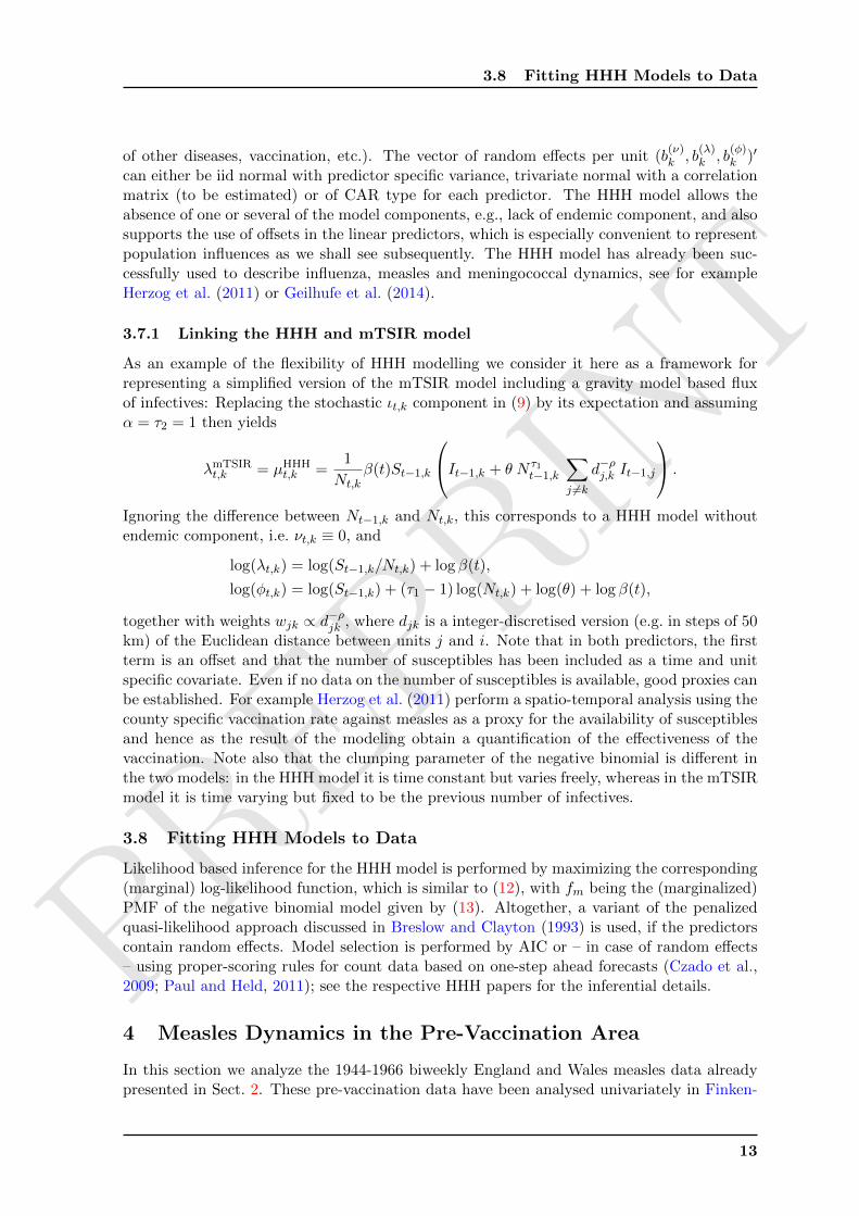
3.7 Endemic-Epidemic Modelling
Inspired by the SIR and mTSIR model, Held et al. (2005) presented a multivariate countdata time series model for routine surveillance data, which does not require the number ofsusceptibles to be available. The formal inspiration for the model was the spatial branchingprocess with immigration, which means that observation time and generation time have tocorrespond. In a series of successive papers the modelling was subsequently extended suchthat it now constitutes a powerful and flexible regression approach for multivariate count datatime series (Paul et al., 2008; Paul and Held, 2011; Held and Paul, 2012; Meyer and Held,2014). From a spatial statistics perspective this even includes the use of CAR type randomeffects (Besag et al., 1991) in the time series modelling. The fundamental idea is to divide theinfection dynamics into two components: an endemic component handles the influx of newinfections from external sources and an epidemic component covers the contagious nature byletting the expected number of transmissions be a function of the lag-one number of infections.The resulting so called HHH model is given by:
Yt,k ∼ NB(µt,k, γk), t = 2, . . . , T, k = 1, . . . ,K, (13)
µt,k = Nt,k νt,k + λt,k Yt−1,k + φt,k∑j 6=k
wjk Yt−1,j .
In the above, Yt,k denotes the number of new cases in unit k at time t which is assumedto follow a negative binomial distribution with expectation µt,k and region specific clumpingparameter γk. As before, Nt,k denotes the corresponding population in region k at time tand the wjk are known weights describing the impact of cases in unit j on unit k. Thiscan, for example, be population flux data such as airline passenger data (Paul et al., 2008)or neighbourhood indicators such as wjk ∝ I(djk = 1) or a power-law weight wjk ∝ d−ρjk ,where in the later two examples djk denotes the graph-based distance between units j andk in the neighbourhood graph while ρ is a parameter to estimate (Meyer and Held, 2014).Furthermore, νt,k, λt,k and φt,k are linear predictors covering the endemic component as wellas the within and between unit auto-regressive behaviour, respectively,
log(νt,k) = α(ν) + b(ν)k + z
(ν)t,k
′β(ν),
log(λt,k) = α(λ) + b(λ)k + z
(λ)t,k
′β(λ),
log(φt,k) = α(φ) + b(φ)k + z
(φ)t,k
′β(φ).
In each case, α(·) denotes the overall intercept, b(·)k a unit-specific random intercept and z
(·)t,k
represents a length p(·) vector of possibly time-varying predictor specific covariates with asso-ciated parameter vector β(·). The use of covariates allows for a flexible modelling of, e.g., secu-lar trends and concurrent processes influencing the disease dynamics (temperature, occurence
12
PREPRINT
3.8 Fitting HHH Models to Data
of other diseases, vaccination, etc.). The vector of random effects per unit (b(ν)k , b
(λ)k , b
(φ)k )′
can either be iid normal with predictor specific variance, trivariate normal with a correlationmatrix (to be estimated) or of CAR type for each predictor. The HHH model allows theabsence of one or several of the model components, e.g., lack of endemic component, and alsosupports the use of offsets in the linear predictors, which is especially convenient to representpopulation influences as we shall see subsequently. The HHH model has already been suc-cessfully used to describe influenza, measles and meningococcal dynamics, see for exampleHerzog et al. (2011) or Geilhufe et al. (2014).
3.7.1 Linking the HHH and mTSIR model
As an example of the flexibility of HHH modelling we consider it here as a framework forrepresenting a simplified version of the mTSIR model including a gravity model based fluxof infectives: Replacing the stochastic ιt,k component in (9) by its expectation and assumingα = τ2 = 1 then yields
λmTSIRt,k = µHHH
t,k =1
Nt,kβ(t)St−1,k
It−1,k + θ N τ1t−1,k
∑j 6=k
d−ρj,k It−1,j
.
Ignoring the difference between Nt−1,k and Nt,k, this corresponds to a HHH model withoutendemic component, i.e. νt,k ≡ 0, and
log(λt,k) = log(St−1,k/Nt,k) + log β(t),
log(φt,k) = log(St−1,k) + (τ1 − 1) log(Nt,k) + log(θ) + log β(t),
together with weights wjk ∝ d−ρjk , where djk is a integer-discretised version (e.g. in steps of 50km) of the Euclidean distance between units j and i. Note that in both predictors, the firstterm is an offset and that the number of susceptibles has been included as a time and unitspecific covariate. Even if no data on the number of susceptibles is available, good proxies canbe established. For example Herzog et al. (2011) perform a spatio-temporal analysis using thecounty specific vaccination rate against measles as a proxy for the availability of susceptiblesand hence as the result of the modeling obtain a quantification of the effectiveness of thevaccination. Note also that the clumping parameter of the negative binomial is different inthe two models: in the HHH model it is time constant but varies freely, whereas in the mTSIRmodel it is time varying but fixed to be the previous number of infectives.
3.8 Fitting HHH Models to Data
Likelihood based inference for the HHH model is performed by maximizing the corresponding(marginal) log-likelihood function, which is similar to (12), with fm being the (marginalized)PMF of the negative binomial model given by (13). Altogether, a variant of the penalizedquasi-likelihood approach discussed in Breslow and Clayton (1993) is used, if the predictorscontain random effects. Model selection is performed by AIC or – in case of random effects– using proper-scoring rules for count data based on one-step ahead forecasts (Czado et al.,2009; Paul and Held, 2011); see the respective HHH papers for the inferential details.
4 Measles Dynamics in the Pre-Vaccination Area
In this section we analyze the 1944-1966 biweekly England and Wales measles data alreadypresented in Sect. 2. These pre-vaccination data have been analysed univariately in Finken-
13

PREPRINT
4 Measles Dynamics in the Pre-Vaccination Area
stadt and Grenfell (2000) and Finkenstadt et al. (2002) and are available for download fromthe internet (Grenfell, 2006). The present analysis is an attempt to analyse the data inspatio-temporal fashion. In a pre-processing step we determine S1,k for each of the 60 seriesas follows: the linear model (11) is fitted for a grid of S1,k values and the resulting log-
likelihood is used to determine S1,k. Subsequently, the recursion in (10) is used to compute
the time series of susceptibles in unit k given S1,k. Figure 3 shows this exemplarily for thetime series of London.
0e+00 2e+05 4e+05
26.5
27.0
27.5
28.0
28.5
29.0
S1,London
Logl
ikel
ihoo
d
050
000
1500
0025
0000
Time (biweek)
St,L
ondo
n
1944 1949 1954 1959 1964
Figure 3: (left) Loglikelihood of the linear model as a function of S1,k for London. (right)Resulting time series of susceptibles obtained from the S1,k maximizing the loglikelihood.
4.1 Results of the mTSIR Model
We use the individually reconstructed series of susceptibles for each city to fit the mTSIRmodel to the multivariate time series of the 60 cities. Fitting the model based on the likelihoodproves to be a complicated matter: We therefore follow the strategy of Xia et al. (2004)by fixing β(t) to the 26 parameters found in Finkenstadt and Grenfell (2000) and fixingα = 0.97. Table 1 contains the ML results in a model where the ιt,k variables are replacedwith their expectation. The table also contains 95% Wald confidence intervals (CI) based onthe observed inverse Fisher information.
Estimate 2.5% 97.5%
τ1 2.24 2.24 2.24τ2 1.10 1.10 1.10ρ 3.05 · 10−2 2.94 · 10−2 3.16 · 10−2
θ 1.79 · 10−16 1.77 · 10−16 1.81 · 10−16
Table 1: Parameter estimates and 95% CIs for the mTSIR model.
Altogether, the results differ quite markedly from the results reported in Xia et al. (2004),where the estimates are τ1 ≈ 1, τ2 ≈ 1.5, ρ ≈ 1 and θ ≈ 4.6·10−9. Several explanations for thedifferences exist: different estimation approaches and different data were used. Altogether,
14

PREPRINT
4.2 Results of the HHH modelling
it appears that the full mTSIR model appears too flexible for the available reduced data setcontaining only 60 cities. Still, the one-step ahead 95% predictive distributions obtained byplug-in of the MLE show that the model enables too little variation: a substantial numberof observations lay outside the 95% predictive intervals obtained by computing the 2.5% and97.5% quantile of the truncated negative-binomial in (9). Fig. 4 shows this exemplarily for theLondon time series. One explanation might be the direct use of It−1,k as clumping parameterfor the negative binomial distribution in (9) – it appears more intuitive that the variance withincreasing It−1,k should increase instead of converging to the Poisson variance as implied bythe model.
050
0010
000
1500
0
Cas
es
1944 1946 1948 1950 1952 1954 1956 1958 1960 1962 1964 1966
Observed1−step−ahead 95% PI
Figure 4: One-step ahead 95% predictive intervals for the London time series obtained byplug-in of the MLE in the mTSIR model. Also shown is the actual observed time series.
4.2 Results of the HHH modelling
Instead of trying to improve the mTSIR model manually, we do so by performing this in-vestigation within the HHH model. As initial HHH model capturing seasonality in both theendemic and epidemic components we consider the following model:
log(νt,k) = log(Nt,k) + α(ν) + β(ν)1 sin
(2πt
26
)+ β
(ν)2 cos
(2πt
26
),
log(λt,k) = α(λ) + β(λ) log(Nt,k) + β(λ)1 sin
(2πt
26
)+ β
(λ)2 cos
(2πt
26
),
log(φt,k) = α(φ) + β(φ) log(Nt,k) + β(φ)1 sin
(2πt
26
)+ β
(φ)2 cos
(2πt
26
),
and with weights wjk = I(0 < distjk ≤ 50km), where distjk denotes the geographic distancebetween cities j and k in km. As a first step in our model selection strategy we compare thismodel to one using weights wjk = d−ρjk , which corresponds to a power-law distance relationshipwith djk = ddistjk /50kme. Based on AIC such a power-law distance kernel is prefered (AIC3.172·105 vs. 3.189·105) and we hence proceed analysing the power-law version. Figure 5 showsthe model fit decomposed into the three components exemplarily for the three largest andthree smallest cities. We observe that the endemic and neighbourhood components only playa small role in the measles transmission. However, neither exluding the endemic component(AIC 3.1981 · 105) nor exluding the neighbourhood component (AIC 3.1977 · 105) provides
15

PREPRINT
4 Measles Dynamics in the Pre-Vaccination Area
a better AIC. Furthermore, Fig. 6 shows the weight quantifying neighbourhood interaction
1945 1950 1955 1960 1965
0
2000
4000
6000
8000
No.
infe
cted
Birmingham
●●●●●●●●●●●●●●●●●●●●●●●
●
●
●
●
●
●
●
●
●
●
●
●●●●●●●●●●●●●●●●●●●●●●●●
●●●●●●
●●●●●
●●●●●●●●
●
●
●
●●
●
●
●
●●●●●●●●●●●●●●●●●●●●●
●
●
●
●●●●
●
●
●
●
●
●
●●●●●●●●●●
●●●
●
●
●
●●
●●●●●
●
●●●
●●●●●●●●●●●●●●●
●●●●●
●●
●
●●●
●
●●●●●●●●
●●
●●
●
●
●●●●
●
●
●
●
●
●
●●●●●●●●●
●●●●●●
●●●●●●●●●●●●●●●●●
●
●
●
●
●
●●
●
●
●
●
●
●
●
●●●●●●●●●●●●●●●●●●●●●●●●●●●●●●●●●●●●●●●●●●
●●
●
●
●
●
●
●●
●
●
●
●
●
●
●●●●●●●●●●●●●●●●●●●●●●●●●●●●●●●●●●
●●●●●●●
●
●
●
●
●
●
●
●
●
●
●●
●
●●●●●●●●●●●●
●●●●●●●●●●●●
●●
●
●●●●●●●●●
●
●
●
●●●
●
●
●●●
●●
●●
●●●●●●●●●●●●●●●●●●●●●●●●●●●●●●●●
●●●●
●
●●
●
●
●●
●●
●
●
●
●●
●●
●●●●●●●●●●●●●●●●●●
●●●●●●●●●●●●●●●●
●
●●
●
●
●●
●●
●
●
●
●●●
●●●●●●●●●●●●●●
●●●●●●●●●●●●●●
●●
●
●●●●●●●
●●
●
●
●
●●●●●●
●●●●●●●
●●●●●●●●●●●●●●●●●●●●●●●●●●●●●●●
●
●
●
●●
spatiotemporalautoregressiveendemic
1945 1950 1955 1960 1965
0
500
1000
1500
2000
2500
No.
infe
cted
Liverpool
●●●●●
●
●●
●●
●●●
●
●
●
●●
●
●
●●
●●
●
●
●●
●●
●
●●
●●●●●●●●●●
●●●●●●●●●●
●●●
●●
●
●●
●
●●
●
●
●
●
●●●●●
●●●
●●
●●●●
●●
●
●●
●
●●
●
●
●
●
●
●●●●●●●
●●●●
●
●
●
●
●●
●
●
●
●
●
●
●●●
●●●●●
●●●
●
●
●●
●●●
●●
●●
●
●
●
●
●
●
●●●●●●●●
●
●
●
●
●
●
●
●
●
●
●●
●●
●
●●
●●●●●●●●●●●●
●●●
●
●
●●
●
●
●
●
●
●
●
●
●
●
●
●●●●●●●
●
●
●
●
●●
●
●
●●
●
●
●
●
●
●
●●●●●●●●●●
●●
●
●
●
●
●●
●
●●
●
●
●
●
●
●●●●●●●●●
●●●●●●
●
●●●●●
●●●
●
●
●
●
●●
●
●
●●●
●
●
●●
●●
●●●●●
●●●●
●
●
●●●●●●
●
●●●●●●●●●●
●
●
●
●●
●●
●
●
●
●●●
●
●●●
●
●
●
●
●
●
●
●
●
●
●●
●●
●●
●●
●
●
●●●●●●●●●●
●
●
●●●●●●
●●
●
●
●
●
●
●
●●●
●
●●
●
●
●
●●
●
●
●
●
●●
●●●●●
●
●
●●●●●
●●●●
●●●●
●
●●
●
●●●
●
●
●●
●
●
●
●●●
●
●●●●●
●
●
●
●●
●●
●
●
●●
●●●
●
●
●●
●●●●●●●●●●●●●●
●
●●●●●
●
●
●
●
●
●
●
●
●
●
●
●
●
●
●
●
●
●
●
●●●●●●●●●●●●●●●
●●●
●
●●
●
●●
●
●
●
●●
●●
●
●
●
●
●●
●●
●●●
●●●●●
●●●
●
●
●●
●
●●
●●
●●
●
●
●●●●
●
●
●●
●●
●
●●
●
●
●●●●
●●●
●●●●●
●●●●
●
●
●●
●
1945 1950 1955 1960 1965
0
2000
4000
6000
8000
10000
12000
14000
No.
infe
cted
London
●●●●●●●●●●●●●●●●●●●●●●●●●●●
●
●
●
●
●
●
●
●
●
●
●
●●●●●●●●●●●●●●
●●
●
●
●●
●
●
●
●
●●
●
●
●
●
●
●●●●●●●●●
●●
●●●
●●●
●
●●●●●
●●
●
●●●●●●●●●
●●
●
●
●
●
●
●
●●●●
●
●
●
●
●●●●●●●●●●
●
●
●
●
●
●
●●
●
●
●
●
●
●
●
●
●●●●●●●●●●●●●●
●●●●●
●
●
●●●●●
●
●●●●
●
●
●
●
●
●
●
●
●●
●
●
●
●
●
●
●
●●●●●●●●●●●●●●●●●
●●●●●●●
●
●●●
●
●
●
●
●
●
●
●●
●
●●
●
●
●
●
●
●
●
●
●●●●
●●●●●●●●●●●●●●●●●●●
●●●●●●●●●●●●●●●●●●
●
●
●
●●
●
●
●
●●
●
●
●
●
●
●
●
●●●●●●●●●●●●●●●
●●●●●●
●
●●●●●●●●●●●●●●
●●
●●
●
●
●
●●●
●
●●●
●
●
●●●●●●●●●●●●●●
●●●●●
●●
●
●●●●●
●
●
●●●●
●●●
●●
●
●
●●●
●●
●
●●●
●
●
●
●●●●●●●●●●●●●●●
●●●●●●●●●●●●●●●●●●
●●
●
●
●
●●
●
●●
●●
●
●
●
●
●
●
●●●●●●●●●●●●●●●●
●●●●●●●●●●●●●●●●●●
●
●
●
●●
●
●
●
●●
●
●●
●
●●●
●
●●
●
●
●●●●●●●●●●●●●●●●●●●●●●●●
●
●
●●●●●
●
●
●●
●
●
●
●
●
●
●
●
●
●
●
●
●
●
●●
●●●●●●●●●●●●
●●●●●
●●●
●
●●
●●
●
●
●●●
●
●
●
●
●
●
1945 1950 1955 1960 1965
0
100
200
300
400
500
600
No.
infe
cted
Kings.Lynn
●●●●●
●
●●
●
●●
●●●●●●●
●
●●
●
●●●●●●●●
●
●
●●●●●●●●
●
●
●
●●
●●
●
●●
●●●●
●
●●●●●●●●●●
●●●●●●●●●●●●
●●●●●●●●●●●●●●●●●●●●●●●●●
●
●
●
●
●
●
●
●
●●●●●●●●●●●●●●●●
●●●●●
●●
●
●●●
●
●
●
●
●
●●●
●
●
●●
●
●●●●●●●●●●●●●●●●●●
●●
●
●
●
●
●
●
●●
●
●●●●●●
●
●●●●●●●●●●
●●●●●●●●●●●●●●
●●
●●●
●
●
●
●
●
●
●●●●●●
●●
●●●●●●●●
●
●
●
●●
●
●
●
●●●●●●●●●●●●●●
●
●
●
●
●●●
●
●
●
●
●
●●●●●●●●●●●●●
●
●●
●●●●●●●●●
●
●
●●●●●●●●●●●
●
●●●
●●
●
●
●●●●
●
●●●
●●
●●●●●●●●●
●●●●●●●
●●
●
●
●●
●
●●●●●●●●●●●●●
●●
●
●●
●●●●●
1945 1950 1955 1960 1965
0
50
100
150
200
250
No.
infe
cted
Shrewsbury
●●●●●●●●●
●●
●●●
●
●
●
●
●●●
●
●
●
●●●●●●●
●●●●
●●
●
●
●
●
●
●●●
●●
●
●
●
●●
●
●
●●●●●●●●●●●●●●
●●●●●●●
●
●
●
●
●
●
●●●
●
●
●
●
●
●●●
●●●●●●●●
●
●
●●●
●●
●
●
●
●
●●●●●●●●●●
●
●
●
●
●
●●
●
●
●
●●
●
●
●●●●●●●●
●
●●●●
●
●
●●
●
●●●●●
●
●
●
●
●
●●
●
●
●
●
●●●
●●●●●● ●
●●●●●
●
●
●
●
●
●
●
●
●
●●
●
●
●●●
●●●● ●●●●●●
●●
●
●
●
●
●
●
●●
●
●
●
●
●
●
●●●●●●●●●●●●●●●●●●●●
●
●
●
●
●
●
●
●
●
●●
●●
●
●
●●●●●●●
●
●●●●
●
●
●
●
●
●
●
●
●
●
●
●●
●
●
●●●●
●
●●●●
●●●●
●
●●●●●●●●●●●●
●
●
●●●
●●
●
●
●
●
●
●
●
●
●
●
●●●
●●
●●
●
●
●
●●●●●●●●●●
●●●●●
●●
●
●
●●
●
●
●●
●●
●
●
●
●
●●●●●●●
●
●
●
●
●●
●●●●
●●●
●
●
●
●
●
●
1945 1950 1955 1960 1965
0
50
100
150
200
No.
infe
cted
Teignmouth
●●
●●
●●●●
●
●
●●●
●●●●●
●●●
●
●
●
●
●
●
●●●●●●●●●●●●●●●●●
●●
●
●
●
●●
●
●
●
●
●
●
●●
●
●
●●●●●●●●●●
●
●
●
●
●
●
●●●●
●●●●●●●●●●●
●●
●●
●
●
●
●
●
●
●
●●
● ●●●●●
●
●
●
●
●
●
●
●●●● ●●●●●●●
●
●●
●
●
●
●●●
●
●● ●●
●
●●●
●●
●●
●
●
●
●
●
●
●
●
●
●●●●●●●● ● ●
●●●●●●
●
●
●
●
●
●
●
●
●
●●●●●●●
●●●●●
●
●
●
●
●●
●●
●
●●●●●●●● ●
●●
●
●
●●
●
●●●●●●●●
●
●●
Figure 5: Time series of counts for the three largest (top row) and three smallest (bottomrow) cities. Also shown are the model predicted expectations decomposed into the threecomponents: endemic, within city and from outside cities.
as a function of distance (in steps of 50km). The right panel of the figure contrasts thepowerlaw model with a model containing individual coefficients for lags 1-4; this gives someindication that the distance influence might be stronger at short lags than implied by thepowerlaw model. Also, the AIC of this more flexible model is slightly better (AIC 3.198 ·105).However, there is not enough information in the data to fit individual coefficients for lags 5and higher.
The seasonal component in the two components is best illustrated graphically, c.f. Fig. 7.We note that the seasonality of the dominating within city transmission component hasa shape very similar to what was found in previous work, i.e. with a lower transmissionduring the summer time. On the other hand, during summer time imports from externalsources appear more likely. The interpretation of the neighbourhood transmission is slightlyinconclusive as it is shifted compared to the two other – this component only makes up asmall part of the overall transmission though.
4.3 Results of the mTSIR mimicking HHH model
When α = 1 and the auto-regressive part is just It,k−1+mt,k we can, as described in Sect. 3.7,mimic the behaviour of the mTSIRmodel by using a HHH model with
16

PREPRINT
4.3 Results of the mTSIR mimicking HHH model
djk
wjk
0.00
0.05
0.10
0.15
1 2 3 4 5 6 7 8 9 10 11
●
●
●
●
●
●
●
●●●●
●
●●
●
●●
●
●
●
●●
●●
●
●●
●●
●●● ●
●
●
● ●●
●
●
●
●
●●
●●
●●
●● ●
●
●
●
●
●●
●
●
●
●●
●
●
●
●
●●●●
●
●●● ●
●●
● ●●
●● ●
●
●●●● ●
●● ●●●
● ●●
●
●●
●
●
●
● ●
●
●●
● ●●●
●
●
●●
●●●●● ●●
●
●●
●●●
● ●
●
●●
●●
●● ●●
●
●
●●
●●● ●
●●
●
●
●
●
●●
●
●
●●●
●
●●
●●
●
●
●●●●
●
●●
●
●
●
●●
●
●
●
●
●●● ●
●
●●●
●
●
●
●
●
●●
●
●
●
●●
●
●
●
●● ●●
●
● ●●
●
●
●
●
●●
●●
●●
● ●
●●
●●●
●●
●
●
●
●
●
●●
●
●
●●●●
●
●●●
●●
●
● ●●●
●
●
●
●●
●● ●●● ●●
●
● ●●
●
●
●●●●
● ●
●
●●
●●
●●
●
●●
●
●●
●
●
●
●
●
●
●
●●●●
●
●●
●
●●
●
●
●
●●
●●
●
●●
●●
●●● ●
●
●
● ●●
●
●
●
●
●●
●●
●●
●● ●
●
●
●
●
●●
●
●
●●●
● ●●●
●●
●
●
●●● ●
●
●●● ●
●●●●●
●●
● ● ●
●
● ●● ●
●●
●
●
●
●●●●
●
●
●●● ●
●
●
●●●
●●● ●
●●
●
●
●●
●●●● ●●
●●
●
●
●
●
●●
●●
●
●●
●●●
●
●
●● ●●
●
● ●●
●
●
●
●
●
●●●
●●● ●
●●
●
●●●● ●
●
●●●
●●●
●
●
●● ●●
●
● ●
●
●
●
●●
●●
●●●
●
●
●● ●●● ●●
●
●●
●
●
●
●●●●
●●
●●● ●●
●
● ●●
●●● ●●●
●
●●●
●
●
●
●
●
● ●●●
●
●●●
●●●●
●●
●●
●● ●
●
●●●
●
●●●
●
●
●●●
●
●
●
●●● ●
●
●
●●
●
●●
●●●●
●
● ●●
●
●
●
●●●
●
●●●●
●
●
●
●●
●
●
●
●●
● ● ●●
●
●
●
●
●
●
●
●
●
●●● ●
●
●
●●● ●
● ●●●
●
●●● ●
●●
●
●●●
●
●
●
●
●● ●●●
●
●●● ●●●●
●●●●
●● ●
●
● ●●●
●
●
●
●
●
●●●
●
●
●●●
● ●
●
●
●●
●
●●
●
●
●
●
●●●●
●● ●●
●●
●●
●
●● ●
● ●●
●●●
●
●●●●
●●● ●
●● ● ●●●
●●●●●
● ●
●
●●
●
●
●●
●
●
●●
●●
● ●●
●●●
●
●
●
●
●
●●
●● ●●
●
●●
●
●
●●
●
●●
●● ●●
●
●
●●
●
●
●
●
●
●●● ●
●
●
●●● ●●●
● ●●
● ●● ●●●
●
●●●
●
●●
●●●● ●
●●
●●
●●
●●
●
●
●
●
●
●● ●
●
●
●●
●
●
●●
●
●
●●●
●
●●
●●
●
●
●●●
●
●
●●
●
●●
●
●
●●● ●●
●●●
●●
●
●
●●●●
●
●
●●
●
●●
●●●●
●
●
●
●
●●
●●●
● ●●●●
●●●●
●
●● ●
●
●
●
●●
●●
●●●
●●●
●
●
●●
●
●
● ●● ● ●●● ●●●●● ●
●●● ● ●
●
● ●● ●
●
●
●
●
●
●●●●
●
●●●● ●
●
●
●●●
●●● ●●● ●
● ●● ●●
●●● ●● ●●● ●●●
●●●
●●● ●●●●
●
●●●●● ● ●●● ●
●
●● ● ●●●● ●
●
● ●●
● ●●● ●
●
● ●●
●●●●
●
●
●
●
●●
●
●● ●●●
●
●●
●●
●
●●
●●●●
●
●
●●
● ●●
●● ●
●● ●●
●
●●●● ●●● ●● ●●●●
●
●●
●
●
●
●
●
●●● ●
●
●●
●
●
●
●
●
●●
●
●●
●●
●●
●
●● ●
●
●
● ●●
●
●
●
●
●
●●●
●
●
● ●
●●
●
●●●● ●
●
● ●●● ●● ●
●
●●●
●● ●●●
●
●●●
●
●●●
●●●●●
●
●●●
●● ● ●●● ●
●●
●
● ●●●
●●
●
● ●
●
●●●●●
●
● ●●
●●●●●
●
●
●
●●
●
● ● ●●
●
●●
●
●●
●
●●
●● ●●
●
●
●●
●●
●
●
●
●●● ●●
●
●●● ●●●● ●●
● ●● ●●●
●● ●●
●●
●●
●
●●
●
●●●●
●
●
●
●
●●
●
●●
●● ●●
●
●
●
●●
●●
●
●●
●●
●●
●
●●● ● ● ●● ●●
●●●●
●●●●
●●
●
●
●●● ●●
●●
●
●
●
●
●●
●●●
● ●●●●
●
●● ●
●
●
● ●●
●
●
●
●
●
●●●
●●● ●
●●
●
●●●● ●
●
● ●
●
●●●●●●●
●
●● ●
●●
●●
●
●
●●
●
●●
●
●
●● ●
●
●
●
●
●
●
●●●
●
●●
●● ●●
●●
●
●● ●●
●
●
●●
●●
●
●
●●
●
●
●
●
●●●●
●
●●●
●●
●
● ●●
●● ● ●●●● ●
●● ●●●
● ●●
●
●●
●
●
●
● ●
●
●●
● ●●●
●
●
●●
●●
●●●
● ●●
●
●
●
●
●
●●
●
●●
●●
●
●●
●●
●
●
●
●
● ● ●
●
●
●
●●
●
●
●
●
●
●●●●
●
●
●●● ●●●●●
●●●
● ●●●
●
●●●
●
●
●
●
●
●
●
●
●
● ●●
●
●●
●●
●
●
●
●
● ● ●
●
● ●
●
●
●
●
●
●
●
●●●●
●
●
●●● ●
● ●●●
●
●●
●●
●
●●
●●
●
●
●
●●●
●
●
●●
●
●●
●
●
●
●●
●●●
●●
●
●●●●
●
●
● ●●●
●●
●
●
●
●●
●●
●
● ●●
●●●
●●
●●
●
●●
●
●
●
●
●
●●●●
●
●●
●
●●
●
●
●
●●
●●
●
●●
●
●●● ●
●
●
● ●●
●
●●
●
●●
●●
●●
●● ●
●
●●●
●●
●●
●● ●● ●● ●●
●●● ●● ●●● ●
●
●●●
●●●
●● ●●●● ●●●●● ● ●●● ●
●
●● ● ●●●● ●
●
● ●●
● ●●● ●
●
●●
●
●●●
●
●
●
●
●
●
● ●●
●
●
●●● ●
●●●
●●
●●● ● ●● ●●
●
●●●
●
●
●●●
●
●
●●●
● ●
●
●
●●
●
●●
●●●●
●
● ●●
●
●
●●
●
●●
●
●
●●
●
●
●●
●●
●
●
●
●●
● ● ●●●
●
●
●
●●
●
●
●●●● ●
●
●●● ●
● ●●●
●
●●
●
●● ●
●● ●●
●●
●●
●
●●
●
●● ●●
●
●
●
●●
●●
●
●●
● ●●●
●●●● ●
●●
● ●●● ●●
●
●●● ● ● ●● ●●
●●●●●●
●
● ●● ●●●●
●
●● ●
●
●
●●
●●●
●●●
●
●●
●●●●
●
●
●●●
●●
●● ●
●●
●●●●
●●
●●
●
●
●
●
●●
●●
●
●●
●
●
●
●
●
●●●●
●
●●
●
●●
●
●
●
●●
●
●●
●●
●●
●●● ●
●
● ●●
●
●●
●
●
●●●
●●
●● ●
●
●
●●
●●
●
●
●●
●
● ●●
●
●
●●
●●
●
●●
●
●
●
●
●●
●●
●
●
●
●●
● ● ●
●●
●●
●
●
●
●
●
●●●
●
●
●
●●● ●
●●
●●
●
●●
●●
●●● ●●●
●
●
●●
●
●
● ●● ●
●
●●● ●●●●●●●●● ● ●
●
● ●●●●
●
●●
●●●●
●●●●● ●
●
●
●●● ●●● ●●●●
● ●●
●
●
●
●●●
●
●● ●
●
●●
●●
●●
●●●
●●
● ● ●
●● ●
●●
● ●
●
●
●●●●
●
●
●●● ●
●●
●●●
●●● ●
●
●
●
●
●
●
●
●
●●●●
●
●●●
●●
●
● ●●
●
●
●
●
●●
●
●
●●● ●
●
●
● ●●●
●
●
●●
●●
●
●●
●●
●
●
●
●
●●
●●
●●
●
●●●
●
●
●
●●●
●
●
●●
●
●
●
●●
●●
●
●
●
●●
●● ●
●●
●●
●
●
●
●
● ●●●●
●
●
●●● ●
●●
●●
●
● ●
●●● ● ●●●● ●
●●●● ●● ●●● ●
●
●●●
●●●
●● ●●●●
●
●●●●● ● ●●● ●●● ● ●●●● ●
●
● ●●
● ●●● ●
●
●
●
●
●
●
●
●
●
●●●●
●
●●
●
●●
●
●
●
●●
●●
●
●●
●●
●●● ●
●
●
● ●●
●
●●
●●
●●
●●
●● ●
●
●●●
●●
●
●
●●●●●
●●
●
●●●
●
●
●●
●
●● ●
●●
●
●
●
●
● ●●
●
● ●●
●●
●
●
● ●●●
●●● ●
●●●
●
●●
● ●
●
●
●
●●●●
●●●
●●● ●● ●
●
●
●●
●
●●●
● ●●●
●●●●●
●●●●
●
●●
●●●
●●●
●●
●●
● ● ●●●●
●
●
●●●●
●●
●
●●●
●●●●
●
●
●
●●
●
●
●● ●
●
●●
●●
●●
●●
●
●●
●● ●
●
● ●●
●
●
●
●
●
●
●●●●
●
●●● ●
●●
●●●
● ●●
●●●●
● ●●
●
●
●
●
●
●●
●
● ●●
●
●
●●
●
●
●●
●
●●
●● ●●
●
●
●●
●
●
●
●
●
●●●●
●
●●● ●●●
● ●●
●●● ●
●
●
●
●
●
●
●
●
●●●●
●
●●●
●●
●
● ●●
●
●●
●
●●
●●
●●● ●
●
●
● ●●
●
●
●
●
●●
● ●
●
●● ●
●
●
●
●
●●
●●
●
●●
●
●
●
●
●
●●●●
●
●●
●
●●
●
●
●
●●
●●
●
●●
●●
●●● ●
●
●
● ●●●
●●
●
●
●
●●
●
●
● ●●
●●●
●●
●●
●●●
●●
●●
●●●●●
●
●
●
●
●● ●●
●
●●●●●
●●
●
●●
●●●
●
● ● ●●●
● ●●●●
● ●●
●
●
●
●
●●
●
●●
●
●
●● ●● ●● ●●
●●● ●● ●●● ●
●
●●
●
●●●
●● ●●●●
●
●● ●●● ● ●●● ●
●
●● ● ●●●● ● ● ●●
● ●●● ●
●
●●●
●●●
●
●●
●
●
●
● ●● ●
●
●●● ● ●●●●●●●
●● ●
●
● ●●●
●
●
●
●●
●● ●
● ●
●●●
● ●
●
●●●
●●●
●●●●
●●●
●
●
●●
●
●
● ●● ●
●
●●● ●●●●● ●
●●●● ●
●
● ●●●●
●
●
●
●●●●
●
●
●●●● ●
●
●●●
●●● ●
●●●●●
●●
●
●●●
●●
●●
●
●
●
●
●●
●●
●
●● ●●
●●●
●● ●
●
●
● ●●
●
●
●
●
●
●●●
●●● ●
●●
●●●● ●
●
●
●
●●
●
●
●
●
●● ●●
●
●●●
●●
●
● ●●
●● ●
●
●●●● ●
●● ●●●
● ●●
●
●●
●●
●
●●
●
●●
● ●●●●
●●
●●●●
●
● ●●●●●
●●●●
●
●
●●
●●●● ●●
●
●
●●
●●● ●
●●
●
●
●
●●●
●
●
●●
●●
●●
●●
●
●
●●●●
●●
●
●
●
●
●
●
●
●
●
●
●●●●
●
●●
●
●●
●
● ●●●
●●
●
●●
●●
●●● ●
●
●
● ●●
●
●●
●
●●
● ●
●●
●● ●
●
●
●
●
●
●●
●
●
●
●
●
●
●
●
●●●●
●
●●●
●●
●
● ●●
●
●●
●
●●
●●
●●● ●
●
●
● ●●
●
●
●
●
●●
●●
●●
●● ●
●
●
●
●
●
●●●●
●
●●●●●●
●●
●●
●
●
●●
●●●● ●●
●
●
●●
●●●●
●●
●
●
●
●●●
●
●
●●
●
●
●●
●●
●
●
●●●●
●
●● ●
●● ●
●●
●
●
●
●●●●
●●●
●●
●
●●
●
●●
●
●● ●●●
●●
●● ●●●● ●●● ●
●
●●
● ●●●●
●
●
● ●
●
● ●●● ●
●
●
●
●●
● ● ● ● ● ●
2 4 6 8 10
0.0
0.2
0.4
0.6
0.8
1.0
Neighbourhood order o
Non
−no
rmal
ized
wei
ght
●
●
●
●
● ● ● ● ● ● ●
●
●
Power−law model o−d
Fourth−order model
Figure 6: (left) Normalized weights as a function of djk. (right) Difference between the power-law model and a model containing individual coefficients for each neighbourhood order 1-4and zero weight thereafter.
0 5 10 15 20 25
0.8
0.9
1.0
1.1
1.2
1.3
endemic
biweek
0 5 10 15 20 25
0.8
0.9
1.0
1.1
1.2
ar
biweek
0 5 10 15 20 25
0.8
0.9
1.0
1.1
1.2
1.3
1.4ne
biweek
Figure 7: Illustration of the seasonal terms of the endemic, auto-regressive and neighbourhoodcomponent of the powerlaw HHH model.
log(λt,k) = β(λ)1 sin
(2πt
26
)+ β
(λ)2 cos
(2πt
26
)+ log
(St−1,kNt,k
),
log(φt,k) = log(θ) + β(φ)1 sin
(2πt
26
)+ β
(φ)2 cos
(2πt
26
)+ (τ1 − 1) log(Nt,k) + log(St−1,k),
and wjk = d−ρjk , which corresponds to a power-law distance relationship. In both thesecomponents the last term of the predictor represents an offset – an alternative would have
been to use terms of the type β(.)3 log(St−1,k) in order to address additional non-linearity in
the susceptibles as suggested in the original TSIR formulations (Finkenstadt and Grenfell,2000; Finkenstadt et al., 2002). The results obtained from fitting this model to the 60 citiesdata are given in Tab. 2.
By transformation we find the corresponding mTSIR model parameters to be θ = 2.5 ·10−5 (95% CI: 1.9 · 10−5-3.4 · 10−5), τ1 = 1.10 (95% CI: 1.08-1.13) and ρ = 0.84 (95%
17

PREPRINT
5 Discussion
Estimate 2.5 % 97.5 %
ar.sin(2 * pi * t/26) 1.35 1.20 1.50ar.cos(2 * pi * t/26) 4.12 4.05 4.18
ne.1 -10.58 -10.87 -10.29ne.log(N) 0.10 0.08 0.13
ne.sin(2 * pi * t/26) -0.20 -0.25 -0.15ne.cos(2 * pi * t/26) -1.31 -1.35 -1.27
neweights.d 0.84 0.75 0.93overdisp 2.72 2.68 2.76
Table 2: Parameter estimates and 95% CIs for the mTSIR mimicking HHH model.
CI: 0.75-0.93). It also becomes clear that the clumping parameter of the negative binomial isestimated to be at a very different scale than suggested by the mTSIR model. As an additionalsensitivity analysis we investigate whether the addition of an endemic component of the formlog(νt,k) = log(St,k−1) +α(ν) is mandated. This would indicate that there is additional influxof measles cases from unspecified sources, e.g. imports from other cities than the 60 includedin the analysis. However, and as expected for measles, the AIC of the original model is notimproved by this extension (difference in the loglikelihood almost immeasurable). Altogether,no subtantial improvement over the best fitting model in Sect. 4.2 is seen though.
5 Discussion
Focus in this manuscript was on infectious disease data where disease location was known tooccur at a fixed and known set of units (e.g. cities or county centroids) hence ultimately lead-ing to the analysis of multivariate time series of counts. Underlying, the epidemic process may,however, be continuous in space: For infectious diseases such continuous-space continuous-time models have been developed in, e.g., Lawson and Leimich (2000) as well as Meyer et al.(2012). Other recent advances have been a more direct focus on the actual who-infected-whotransmission chains manifesting as spatio-temporal point patters. This could for example bebased on a covariate augmented network model of the underlying contact structure in thepopulation (Groendyke et al., 2012). Another path is to supplement the reconstruction withavailable microbiological information about the disease strain in the cases, e.g., by taking thedifference in RNA sequences as additional genetic distance metric supplementing spatial dis-tance (Aldrin et al., 2011; Ypma et al., 2012). Others have taken the collapse of geographicalspace even further by visualizing and computing only effective-distances based on, e.g., mo-bility or population flux data (Brockmann and Helbing, 2013). Spatio and spatio-temporalmethods have also been used for the detection of disease clusters (Kulldorff, 2001; Diggleet al., 2005; Lawson and Kleinman, 2005) Another application of spatial methods in infec-tious disease epidemiology has been the source identification of large food-borne outbreaks.Here, point-patters of cases are aligned with knowledge about the spatial and spatio-temporaldistribution of food items or appropriate proxies (Manitz et al., 2014; Kaufman et al., 2014).
In a world of commuting and travelling, ’location’ of a case is at best a ’most likely’ or’average’ of the individuals location over time. In the digital age new data sources emergeallowing an even more exact spatio-temporal tracking of individuals. Hence, location isdestined to become a more dynamic concept in future spatio-temporal epidemic models. Ingeneral and for stigmatizing diseases in particular, positional accuracy is destined to be inconflict with data protection of the individual. It is a matter of discussion and evaluation
18

PREPRINT
References
how the right balance is to be found between the two.
Addressing spatial heterogeneity can be one aspect to improve on the usefulness of epi-demic models, but certainly also complicates the analysis. When such models are used tosupport the decision making processes on intervention, control and vaccination, it is impor-tant to remember how formidable a task the modelling of infectious diseases is and where thelimitations lie. From a statistician’s point of view transmission modelling in practice misses astronger emphasis on parameter estimation, uncertainty handling and model selection. Whilethe modelling community has published high-impact semi-mechanistic models, the concurrentadvances in the field by the statistical community have gone somewhat unnoticed. In the last10 years, though, mechanistic modelling, data science and statistical inference for dynamicprocesses appear to have synthesized more. This means that Markov Chain Monte Carlo,approximate Bayesian computation and plug-and-play simulation methods are now standardinstruments for spatially enriched epidemic models (Mugglin et al., 2002; McKinley et al.,2009; He et al., 2010; Jandarov et al., 2014). Furthermore, flexible open-source R packageshave become available for visualizing, analysing and simulating such epidemic models. Inparticular, the R package surveillance (Hohle et al., 2015) implements both the two com-ponent SIR model and the HHH as illustrated in Meyer et al. (2014). However, with powerfulcomputational tools at hand it is also worthwhile to discuss, how complex models need to bein order to answer the questions they are designed for. Long computation times often implylittle room for model diagnostics or model selection, which is equally important. The powerof mathematical models lies in their abstraction as May (2004) reminds us. What to includeand what to abstract upon in order to make a model relevant requires an interdisciplinaryapproach.
Acknowledgments
Sebastian Meyer, University of Zurich, is thanked for his input and comments on the part ofHHH modelling in this chapter.
References
Abrams, S., P. Beutels, and N. Hens (2014). Assessing mumps outbreak risk in highly vac-cinated populations using spatial seroprevalence data. American Journal of Epidemiol-ogy 179 (8), 1006–1017.
Aldrin, M., T. M. Lyngstad, A. B. Kristoffersen, B. Storvik, Ø. Borgan, and P. A. Jansen(2011). Modelling the spread of infectious salmon anaemia among salmon farms basedon seaway distances between farms and genetic relationships between infectious salmonanaemia virus isolates. Journal of the Royal Society Interface 8 (62), 1346–1356.
Anderson, R. M. and R. M. May (1991). Infectious diseases of humans: dynamics and control.Oxfort University Press.
Andersson, H. and T. Britton (2000). Stochastic Epidemic Models and their Statistical Anal-ysis, Volume 151 of Springer Lectures Notes in Statistics. Springer-Verlag.
Bailey, N. T. J. (1950). A simple stochastic epidemic. Biometrika 37 (3/4), 193–202.
Bailey, N. T. J. (1964). The Elements of Stochastic Processes with Applications to the NaturalSciences. Wiley.
19

PREPRINT
References
Bailey, N. T. J. (1975). The mathematical theory of infectious diseases and its applications.Griffin.
Becker, N. G. (1989). Analysis of Infectious Disease Data. Chapman & Hall/CRC.
Besag, J., J. York, and A. Mollie (1991). Bayesian image restoration, with two applicationsin spatial statistics. Annals of the Institute of Statistical Mathematics 43, 1–59. (withdiscussion).
Bjørnstad, O. N., B. F. Finkenstadt, and B. T. Grenfell (2002). Dynamics of measles epi-demics: Estimating scaling of transmission rates using a time series sir model. EcologicalMonographs 72 (2), 169–184.
Bjørnstad, O. N. and B. T. Grenfell (2008). Hazards, spatial transmission and timing ofoutbreaks in epidemic metapopulations. Environmental and Ecological Statistics 15, 265–277.
Breslow, N. E. and D. G. Clayton (1993). Approximate inference in generalized linear mixedmodels. Journal of the American Statistical Association 88 (421), 9–25.
Britton, T. (2010, May). Stochastic epidemic models: a survey. Mathematical Bio-sciences 225 (1), 24–35.
Brockmann, D. and D. Helbing (2013). The hidden geometry of complex, network-drivencontagion phenomena. Science 342 (6164), 1337–1342.
Cliff, A. and P. Haggett (2004). Time, travel and infection. Britisch Medical Bulletin 69,87–99.
Czado, C., T. Gneiting, and L. Held (2009). Predictive model assessment for count data.Biometrics 65, 1254–1261.
Daley, D. J. and J. Gani (1999). Epidemic Modelling. Cambridge University Press.
Deardon, R., X. Fang, and G. Kwong (2015). Statistical modelling of spatio-temporal in-fectious disease tranmission. In D. Chen, B. Moulin, and J. Wu (Eds.), Analyzing andModeling Spatial and Temporal Dynamics of Infectious Diseases. John Wiley & Sons.
Diekmann, O. and J. A. P. Heesterbeek (2000). Mathematical epidemiology of infectiousdiseases. Wiley.
Diggle, P. (2006). Spatio-temporal point processes, partial likelihood, foot and mouth disease.Statistical Methods in Medical Research 15 (4), 325–336.
Diggle, P. J., B. Rowlingson, and T.-L. Su (2005). Point process methodology for on-linespatio-temporal disease surveillance. Environmetrics 16, 423–34.
Diggle, P. J. and B. S. Rowlingson (1994). A conditional approach to point process modellingof elevated risk. Journal of the Royal Statistical Society, Series A 157 (3), 433–440.
Dohoo, I., W. Martin, and H. Stryhn (2010). Veterinary Epidemiologic Research (2nd ed.).VER Inc.
20

PREPRINT
References
Eggo, R. M., S. Cauchemez, and N. M. Ferguson (2011, Feb). Spatial dynamics of the 1918influenza pandemic in England, Wales and the United States. Journal of the Royal SocietyInterface 8 (55), 233–243.
Erlander, S. and N. F. Stewart (1990). The Gravity Model in Transportation Analysis: Theoryand Extensions. VSP.
Fahrmeir, L. and T. Kneib (2011). Bayesian Smoothing and Regression for Longitudinal,Spatial and Event History Data. Oxford University Press.
Finkenstadt, B. F., O. N. Bjørnstad, and B. T. Grenfell (2002). A stochastic model forextinction and recurrence of epidemics: estimation and inference for measles outbreaks.Biostatistics 3 (4), 493–510.
Finkenstadt, B. F. and B. T. Grenfell (2000). Time series modelling of infectious diseases:a dynamical systems approach. Journal of the Royal Statistical Society, Series C 49 (2),187–205.
Geilhufe, M., L. Held, S. O. Skrøvseth, G. S. Simonsen, and F. Godtliebsen (2014, May).Power law approximations of movement network data for modeling infectious diseasespread. Biometrical Journal 56 (3), 363–382.
Gibson, G. J. and E. Renshaw (1998). Estimating parameters in stochastic compartmentalmodels using Markov chain methods. IMA Journal of Mathematics applied in Medicine &Biology 15, 19–40.
Giesecke, J. (2002). Modern infectious disease epidemiology (2nd ed.). Hodder Arnold.
Gillespie, D. T. (1977). Exact stochastic simulation of coupled chemical reactions. TheJournal of Physical Chemistry 81 (25), 2340–2361.
Gog, J. R., S. Ballesteros, C. Viboud, L. Simonsen, O. N. Bjornstad, J. Shaman, D. L. Chao,F. Khan, and B. T. Grenfell (2014). Spatial Transmission of 2009 Pandemic Influenza inthe US. PLoS Compututational Biology 10 (6), e1003635.
Grenfell, B. T. (2006). TSIR analysis of measles in England and Wales. http:
//www.zoo.cam.ac.uk/zoostaff/grenfell/measles.htm. Available from the Inter-net Archive as http://web.archive.org/web/20060311051944/http://www.zoo.cam.
ac.uk/zoostaff/grenfell/measles.htm.
Grenfell, B. T., O. N. Bjørnstad, and J. Kappey (2001). Travelling waves and spatial hierar-chies in measles epidemics. Nature 414 (6865), 716–723.
Grenfell, B. T., A. Kleczkowski, C. A. Gilligan, and B. M. Bolker (1995). Spatial hetero-geneity, nonlinear dynamics and chaos in infectious diseases. Statistical Methods in MedicalResearch 4 (2), 160–183.
Groendyke, C., D. Welch, and D. R. Hunter (2012, Sep). A network-based analysis of the1861 Hagelloch measles data. Biometrics 68 (3), 755–765.
He, D., E. L. Ionides, and A. A. King (2010). Plug-and-play inference for disease dynamics:measles in large and small populations as a case study. Journal of the Royal SocietyInterface 7 (43), 271–283.
21

PREPRINT
References
Held, L., M. Hohle, and M. Hofmann (2005). A statistical framework for the analysis ofmultivariate infectious disease surveillance data. Statistical Modelling 5, 187–199.
Held, L. and M. Paul (2012). Modeling seasonality in space-time infectious disease surveillancedata. Biometrical Journal 54 (6), 824–843.
Held, L. and M. Paul (2013). Statistical modeling of infectious disease surveillance data.In N. M. M’ikanatha, R. Lynfield, C. A. Van Beneden, and H. de Valk (Eds.), InfectiousDisease Surveillance (2nd ed.). Wiley-Blackwell.
Hens, N., Z. Shkedy, M. Aerts, C. Faes, P. Van Damme, and P. Beutels (2012). ModelingInfectious Disease Parameters Based on Serological and Social Contact Data. Springer.
Herzog, S. A., M. Paul, and L. Held (2011). Heterogeneity in vaccination coverage explainsthe size and occurrence of measles epidemics in German surveillance data. Epidemiologyand Infection 139 (4), 505–515.
Hohle, M. (2009). Additive-multiplicative regression models for spatio-temporal epidemics.Biometrical Journal 51 (6), 961–978.
Hohle, M., E. Jørgensen, and P. O’Neill (2005). Inference in disease transmission experi-ments by using stochastic epidemic models. Journal of the Royal Statistical Society, SeriesC 54 (2), 349–366.
Hohle, M., S. Meyer, and M. Paul (2015). surveillance: Temporal and Spatio-TemporalModeling and Monitoring of Epidemic Phenomena. R package version 1.8-4.
Isham, V. (2004). Stochastic models for epidemics. Technical Report 263, Department ofStatistical Science, University College London. Available as https://www.ucl.ac.uk/
statistics/research/pdfs/rr263.pdf.
Jandarov, R., M. Haran, O. Bjørnstad, and B. Grenfell (2014). Emulating a gravity model toinfer the spatiotemporal dynamics of an infectious disease. Journal of the Royal StatisticalSociety: Series C 63 (3), 423–444.
Kaufman, J., J. Lessler, A. Harry, S. Edlund, K. Hu, J. Douglas, C. Thoens, B. Appel, A. Kas-bohrer, and M. Filter (2014). A likelihood-based approach to identifying contaminatedfood products using sales data: performance and challenges. PLoS Comput. Biol. 10 (7),e1003692.
Keeling, M. J., O. N. Bjørnstad, and B. T. Grenfell (2004). Chapter 17 - metapopulationdynamics of infectious diseases. In I. Hanski and O. E. Gaggiotti (Eds.), Ecology, Geneticsand Evolution of Metapopulations, pp. 415 – 445. Burlington: Academic Press.
Keeling, M. J. and P. Rohani (2008). Modeling Infectious Diseases in Humans and Animals.Princeton University Press.
Kermack, W. O. and A. G. McKendrick (1927). A contribution to the mathematical theoryof epidemics. Proceedings of the Royal Society, Series A 115, 700–721.
Klinkenberg, D., J. de Bree, H. Laevens, and M. C. M. de Jong (2002). Within- and between-pen transmission of classical swine fever virus: a new method to estimate the basic repro-duction ratio from transmission experiments. Epidemiology and Infection 128, 293–299.
22

PREPRINT
References
Kulldorff, M. (2001). Prospective time periodic geographical disease surveillance using a scanstatistic. Journal of the Royal Statistical Society, Series A 164, 61–72.
Lau, M. S. Y., G. Marion, G. Streftaris, and G. J. Gibson (2014). New model diagnosticsfor spatio-temporal systems in epidemiology and ecology. Journal of The Royal SocietyInterface 11 (93).
Lawson, A. and K. Kleinman (Eds.) (2005). Spatial and Syndromic Surveillance for PublicHealth. Wiley.
Lawson, A. and P. Leimich (2000). Approaches to the space-time modelling of infectiousdisease behaviour. IMA Journal of Mathematics Applied in Medicine and Biology 17 (1),1–13.
Liu, W., H. W. Hethcote, and S. A. Levin (1987). Dynamical behavior of epidemiologicalmodels with nonlinear incidence rates. Journal of Mathematical Biology 25, 359–380.
Madden, L. V., G. Hughes, and F. van den Bosch (2007). The Study of Plant DiseaseEpidemics. APS Press.
Manitz, J., T. Kneib, M. Schlather, D. Helbing, and D. Brockmann (2014). Origin DetectionDuring Food-borne Disease Outbreaks - A Case Study of the 2011 EHEC/HUS Outbreakin Germany. PLoS Currents 6.
May, R. M. (2004). Uses and abuses of mathematics in biology. Science 303 (5659), 790–793.
McKinley, T. J., A. R. Cook, and R. Deardon (2009). Inference in epidemic models withoutlikelihoods. The International Journal of Biostatistics 5 (1), Article 24.
Meyer, S., J. Elias, and M. Hohle (2012). A space-time conditional intensity model for invasivemeningococcal disease occurrence. Biometrics 68 (2), 607––616.
Meyer, S. and L. Held (2014). Modelling power-law spread of infectious diseases. Annals ofApplied Statistics 8 (3), 1612–1639.
Meyer, S., L. Held, and M. Hohle (2014). Spatio-temporal analysis of epidemic phenomenausing the R package surveillance. Available as http://arxiv.org/pdf/1411.0416.
Morton, A. and B. Finkenstadt (2005). Discrete time modelling of disease incidence timeseries by using Markov chain Monte Carlo methods. Journal of the Royal Statistical Soceity,Series C 54 (3), 575–594.
Mugglin, A. S., N. Cressie, and I. Gemmell (2002). Hierarchical statistical modelling ofinfluenza epidemic dynamics in space and time. Statistics in Medicine 21 (18), 2703–2721.
Neal, P. and G. O. Roberts (2004). Statistical inference and model selection for the 1861Hagelloch measles epidemic. Biostatistics 5 (2), 249–261.
O’Neill, P. D. and N. G. Becker (2001). Inference for an epidemic when susceptibility varies.Biostatistics 2 (1), 99–108.
O’Neill, P. D. and G. O. Roberts (1999). Bayesian inference for partially observed stochasticepidemics. Journal of the Royal Statistal Society, Series A 162, 121–129.
23

PREPRINT
References
Paul, M. and L. Held (2011). Predictive assessment of a non-linear random effects modelfor multivariate time series of infectious disease counts. Statistics in Medicine 30 (10),1118–1136.
Paul, M., L. Held, and A. M. Toschke (2008). Multivariate modelling of infectious diseasesurveillance data. Statistics in Medicine 27, 6250–6267.
Pitzer, V. E., C. Viboud, L. Simonsen, C. Steiner, C. A. Panozzo, W. J. Alonso, M. A.Miller, R. I. Glass, J. W. Glasser, U. D. Parashar, and B. T. Grenfell (2009). Demo-graphic variability, vaccination, and the spatiotemporal dynamics of rotavirus epidemics.Science 325 (5938), 290–294.
R Core Team (2014). R: A Language and Environment for Statistical Computing. Vienna,Austria: R Foundation for Statistical Computing.
Renshaw, E. (1991). Modelling Biological Populations in Space and Time. Cambridge Uni-versity Press.
Riley, S., K. Eames, V. Isham, D. Mollison, and P. Trapman (2014). Five challenges for spatialepidemic models. Epidemics. Epub ahead of print, DOI doi:10.1016/j.epidem.2014.07.001.
Scheel, I., M. Aldrin, A. Frigessi, and P. Jansen (2007). A stochastic model for infectioussalmon anemia (ISA) in Atlantic salmon farming. Journal of the Royal Society Interface 4,699––706.
Smyth, G. K. (1998). Numerical integration. In P. Armitage and T. Colton (Eds.), Encyclo-pedia of Biostatistics, pp. 3088–3095. Wiley.
Viboud, C., O. N. Bjørnstad, D. L. Smith, L. Simonsen, M. A. Miller, and B. T. Gren-fell (2006). Synchrony, waves, and spatial hierarchies in the spread of influenza. Sci-ence 312 (5772), 447–451.
Weidemann, F., M. Dehnert, J. Koch, O. Wichmann, and M. Hohle (2014). Bayesian param-eter inference for dynamic infectious disease modelling: rotavirus in Germany. Statisticsin Medicine 33 (9), 1580–1599.
Wilking, H., M. Hohle, E. Velasco, M. Suckau, and T. Eckmanns (2012). Ecological analysisof social risk factors for rotavirus infections in Berlin, Germany, 2007-2009. InternationalJournal of Health Geographics 11 (1), 37.
Wilkinson, D. J. (2006). Stochastic Modelling for Systems Biology. Chapman & Hall/CRC.
Xia, Y., O. N. Bjørnstad, and B. T. Grenfell (2004, Aug). Measles metapopulation dynamics:a gravity model for epidemiological coupling and dynamics. American Naturalist 164 (2),267–281.
Ypma, R. J., A. M. Bataille, A. Stegeman, G. Koch, J. Wallinga, and W. M. van Ballegooijen(2012). Unravelling transmission trees of infectious diseases by combining genetic andepidemiological data. Proc. Biol. Sci. 279 (1728), 444–450.
24