Embed Size (px)
Citation preview
Inertially Stabilized Platforms for
SATCOM On-The-Move Applications:
A Hybrid Open/Closed-Loop Antenna Pointing
Strategyby
Eric Allen MarshB.S. Mechanical Engineering
United States Air Force Academy, 2006Submitted to the Department of Aeronautics and Astronautics
in partial fulfillment of the requirements for the degree ofMaster of Science in Aeronautics and Astronautics
at theMASSACHUSETTS INSTITUTE OF TECHNOLOGY
June 2008c© Massachusetts Institute of Technology 2008. All rights reserved.
Author . . . . . . . . . . . . . . . . . . . . . . . . . . . . . . . . . . . . . . . . . . . . . . . . . . . . . . . . . . . . . .Department of Aeronautics and Astronautics
June 6, 2008
Certified by. . . . . . . . . . . . . . . . . . . . . . . . . . . . . . . . . . . . . . . . . . . . . . . . . . . . . . . . . .Dr. Dan Asta
Group Leader, MIT Lincoln LaboratoryThesis Supervisor
Certified by. . . . . . . . . . . . . . . . . . . . . . . . . . . . . . . . . . . . . . . . . . . . . . . . . . . . . . . . . .Dr. Timothy Gallagher
Technical Staff, MIT Lincoln LaboratoryThesis Supervisor
Certified by. . . . . . . . . . . . . . . . . . . . . . . . . . . . . . . . . . . . . . . . . . . . . . . . . . . . . . . . . .Prof. Jonathan P. How
Professor of Aeronautics & AstronauticsThesis Supervisor
Accepted by . . . . . . . . . . . . . . . . . . . . . . . . . . . . . . . . . . . . . . . . . . . . . . . . . . . . . . . . .Prof. David L. Darmofal
Associate Department Head, Chair, Committee on Graduate Students

Report Documentation Page Form ApprovedOMB No. 0704-0188
Public reporting burden for the collection of information is estimated to average 1 hour per response, including the time for reviewing instructions, searching existing data sources, gathering andmaintaining the data needed, and completing and reviewing the collection of information. Send comments regarding this burden estimate or any other aspect of this collection of information,including suggestions for reducing this burden, to Washington Headquarters Services, Directorate for Information Operations and Reports, 1215 Jefferson Davis Highway, Suite 1204, ArlingtonVA 22202-4302. Respondents should be aware that notwithstanding any other provision of law, no person shall be subject to a penalty for failing to comply with a collection of information if itdoes not display a currently valid OMB control number.
1. REPORT DATE 02 JUN 2008
2. REPORT TYPE N/A
3. DATES COVERED -
4. TITLE AND SUBTITLE Inertially Stabilized Platforms for SATCOM On-The-Move Applications:A Hybrid Open/Closed-Loop Antenna Pointing Strategy
5a. CONTRACT NUMBER
5b. GRANT NUMBER
5c. PROGRAM ELEMENT NUMBER
6. AUTHOR(S) 5d. PROJECT NUMBER
5e. TASK NUMBER
5f. WORK UNIT NUMBER
7. PERFORMING ORGANIZATION NAME(S) AND ADDRESS(ES) Massachusetts Institute of Technology
8. PERFORMING ORGANIZATIONREPORT NUMBER CI08-0015
9. SPONSORING/MONITORING AGENCY NAME(S) AND ADDRESS(ES) The Department of the Air Force AFIT/ENEL, Bldg 16 2275 D StreetWPAFB, OH 45433
10. SPONSOR/MONITOR’S ACRONYM(S)
11. SPONSOR/MONITOR’S REPORT NUMBER(S)
12. DISTRIBUTION/AVAILABILITY STATEMENT Approved for public release, distribution unlimited
13. SUPPLEMENTARY NOTES The original document contains color images.
14. ABSTRACT
15. SUBJECT TERMS
16. SECURITY CLASSIFICATION OF: 17. LIMITATION OF ABSTRACT
UU
18. NUMBEROF PAGES
216
19a. NAME OFRESPONSIBLE PERSON
a. REPORT unclassified
b. ABSTRACT unclassified
c. THIS PAGE unclassified
Standard Form 298 (Rev. 8-98) Prescribed by ANSI Std Z39-18

2
Inertially Stabilized Platforms for
SATCOM On-The-Move Applications:
A Hybrid Open/Closed-Loop Antenna Pointing Strategy
by
Eric Allen Marsh
Submitted to the Department of Aeronautics and Astronauticson June 6, 2008, in partial fulfillment of the
requirements for the degree ofMaster of Science in Aeronautics and Astronautics
Abstract
The increasing need for timely information in any environment has led to the development of mobileSATCOM terminals. SATCOM terminals seeking to achieve high data-rate communications requireinertial antenna pointing to within fractions of a degree. The base motion of the antenna platformcomplicates the pointing problem and must be accounted for in mobile SATCOM applications. An-tenna Positioner Systems (APSs) provide Inertially Stabilized Platforms (ISPs) for accurate antennapointing and may operate in either an open or closed-loop fashion. Closed-loop antenna pointingstrategies provide greater inertial pointing accuracies but typically come at the expense of morecomplex and costly systems. This thesis defines a nominal two-axis APS used on an EHF SAT-COM terminal on a 707 aircraft. The nominal APS seeks to accomplish mobile SATCOM usingthe simplest possible system; therefore, the system incorporates no hardware specific to closed-looppointing. This thesis demonstrates that the nominal APS may achieve accurate antenna pointingfor an airborne SATCOM application using a hybrid open/closed-loop pointing strategy.
The nominal APS implements the hybrid pointing strategy by employing an open-loop pedestalfeedback controller in conjunction with a step-tracking procedure. The open-loop feedback controlleris developed using optimal control techniques, and the pointing performance of the controller withthe nominal APS is determined through simulation. This thesis develops closed-loop step-trackingalgorithms to compensate for open-loop pointing errors. The pointing performance of several step-tracking algorithms is examined in both spatial pull-in and tracking simulations in order to determinethe feasibility of employing hybrid pointing strategies on mobile SATCOM terminals.
Keywords: Mobile SATCOM, Antenna Pointing, Inertially Stabilized Platform, Two-axis Po-sitioner, Linear Quadratic Gaussian Control, Nonlinear Optimization
Thesis Supervisor: Dr. Dan AstaTitle: Group Leader, MIT Lincoln Laboratory
Thesis Supervisor: Dr. Timothy GallagherTitle: Technical Staff, MIT Lincoln Laboratory
Thesis Supervisor: Prof. Jonathan P. HowTitle: Professor of Aeronautics & Astronautics
3

4

Acknowledgments
First off, I would like to thank Timothy Gallagher for his continued support, guid-
ance, and encouragement in this research. I would also like to thank Dan Asta and
Jonathon How for their contributions and support. A very special thanks is extended
to John Kuconis for my sponsorship at MIT Lincoln Laboratory. The help I received
from Mike Boulet and Anthony Hotz proved invaluable to this research, and their
willingness to answer countless questions has been much appreciated. I would like
to thank the following Lincoln Laboratory employees who have contributed in some
way to this thesis or have at least given me a smile in the hallways: Kevin Kelly,
Ed Bucher, Ross Conrad, Mark Deluca, Rajesh Viswanathan, Nagabushan Sivanan-
jaiah, Mike Gridley, Ted O’Connell, Saunak Shah, John Sultana, John Choi, Misha
Ivanov, Steve Targonski, David Savilonis, Dave Genovese, Peggy Speranza, and Rosa
Figueroa. This list is by no means complete, and I would like to express my deepest
gratitude toward all those who have made my tenure at MIT and Lincoln Laboratory
most enjoyable. Last, but not least, I want to extend a warm thank you to my family
and friends. Without you, none of this matters.
Disclaimer
The views expressed in this article are those of the author and do not reflect the
official policy or position of the United States Air Force, Department of Defense, or
the United States Government.
5

6

Contents
List of Figures 10
List of Tables 14
1 Introduction 17
1.1 Motivation for Work . . . . . . . . . . . . . . . . . . . . . . . . . . . 17
1.2 Problem Statement . . . . . . . . . . . . . . . . . . . . . . . . . . . . 19
1.3 Contributions . . . . . . . . . . . . . . . . . . . . . . . . . . . . . . . 20
1.4 Thesis Overview . . . . . . . . . . . . . . . . . . . . . . . . . . . . . . 21
2 Background and System Architecture 23
2.1 APS Hardware Configurations . . . . . . . . . . . . . . . . . . . . . . 24
2.1.1 APS Components . . . . . . . . . . . . . . . . . . . . . . . . . 24
2.1.2 Antenna Payloads . . . . . . . . . . . . . . . . . . . . . . . . . 24
2.1.3 Pedestals and Sensors . . . . . . . . . . . . . . . . . . . . . . 29
2.1.4 APS Design Requirements . . . . . . . . . . . . . . . . . . . . 32
2.2 Control Strategies . . . . . . . . . . . . . . . . . . . . . . . . . . . . . 33
2.2.1 Open-loop Pointing and Sources of Error . . . . . . . . . . . . 34
2.2.2 Closed-Loop Antenna Pointing Methods . . . . . . . . . . . . 35
2.3 Nominal APS System Architecture . . . . . . . . . . . . . . . . . . . 38
3 Open-Loop Controller Development 41
3.1 Equations of Motion . . . . . . . . . . . . . . . . . . . . . . . . . . . 42
3.1.1 Response Side . . . . . . . . . . . . . . . . . . . . . . . . . . . 42
7
3.1.2 Moment Side . . . . . . . . . . . . . . . . . . . . . . . . . . . 43
3.1.3 Base Motion Disturbance Modeling . . . . . . . . . . . . . . . 46
3.1.4 Linear Plant Model . . . . . . . . . . . . . . . . . . . . . . . . 49
3.2 Controller Development and Simulation . . . . . . . . . . . . . . . . . 51
3.2.1 Linear-Quadratic Regulation Theory . . . . . . . . . . . . . . 52
3.2.2 Linear-Quadratic Estimation Theory . . . . . . . . . . . . . . 54
3.2.3 Linear-Quadratic Gaussian Theory . . . . . . . . . . . . . . . 56
3.2.4 Reference Commands . . . . . . . . . . . . . . . . . . . . . . . 56
3.2.5 Development of the LQG Pedestal Controller in
MATLAB . . . . . . . . . . . . . . . . . . . . . . . . . . . . . 57
3.2.6 Controlled Nonlinear Plant Simulation . . . . . . . . . . . . . 63
3.3 Pointing Error Distributions . . . . . . . . . . . . . . . . . . . . . . . 73
4 Closed-Loop Pointing Strategy 79
4.1 Defining the Cost Function . . . . . . . . . . . . . . . . . . . . . . . . 80
4.2 Facets of the Optimization Problem . . . . . . . . . . . . . . . . . . . 83
4.3 Step-tracking Using Function Comparison Methods . . . . . . . . . . 84
4.3.1 Full-field Search . . . . . . . . . . . . . . . . . . . . . . . . . . 84
4.3.2 Spiral Search . . . . . . . . . . . . . . . . . . . . . . . . . . . 85
4.4 Step-tracking Using Optimization Techniques . . . . . . . . . . . . . 88
4.4.1 Modified Newton’s Method . . . . . . . . . . . . . . . . . . . . 90
4.4.2 Quasi-Newton’s Methods . . . . . . . . . . . . . . . . . . . . . 93
4.4.3 Method of Steepest Descent . . . . . . . . . . . . . . . . . . . 94
4.4.4 Step-tracking Algorithm Architecture . . . . . . . . . . . . . . 95
4.5 Spatial Pull-in Simulations . . . . . . . . . . . . . . . . . . . . . . . . 103
4.5.1 Observations . . . . . . . . . . . . . . . . . . . . . . . . . . . 111
4.6 Spatial Pull-in Robustness Tests . . . . . . . . . . . . . . . . . . . . . 113
4.6.1 Observations . . . . . . . . . . . . . . . . . . . . . . . . . . . 114
4.7 A Look at Tracking . . . . . . . . . . . . . . . . . . . . . . . . . . . . 116
4.7.1 Observations . . . . . . . . . . . . . . . . . . . . . . . . . . . 118
8
4.8 Simulation Processing Times . . . . . . . . . . . . . . . . . . . . . . . 118
5 Conclusions 121
5.1 Open-loop Controller Simulation Results Summary . . . . . . . . . . 121
5.2 Closed-loop Step-tracking Simulation Results Summary . . . . . . . . 122
5.3 Overall Contributions . . . . . . . . . . . . . . . . . . . . . . . . . . . 124
5.4 Suggestions for Future Work . . . . . . . . . . . . . . . . . . . . . . . 125
A Satellite Look Angle Calculations 127
A.1 Satellite Targeting Using Classical Orbital Element Sets . . . . . . . . 128
A.2 Targetting Using Known Inertial Look Angles . . . . . . . . . . . . . 132
A.3 Keplar2RRR.m . . . . . . . . . . . . . . . . . . . . . . . . . . . . . . 134
A.4 basemotionlatlongalt2ECINAVDATA.m . . . . . . . . . . . . . . . . . 136
B Open-Loop Controller Simulations 139
B.1 controller.m . . . . . . . . . . . . . . . . . . . . . . . . . . . . . . . . 139
B.2 APS Simulink Model . . . . . . . . . . . . . . . . . . . . . . . . . . . 143
C Step-tracking Simulations 149
C.1 spiralsearch.m . . . . . . . . . . . . . . . . . . . . . . . . . . . . . . . 149
C.2 modifiedNewton.m . . . . . . . . . . . . . . . . . . . . . . . . . . . . 154
C.3 BFGS.m . . . . . . . . . . . . . . . . . . . . . . . . . . . . . . . . . . 166
C.4 DFP.m . . . . . . . . . . . . . . . . . . . . . . . . . . . . . . . . . . . 180
C.5 steepestdescent.m . . . . . . . . . . . . . . . . . . . . . . . . . . . . . 194
C.6 getsignalpower.m (Subroutine) . . . . . . . . . . . . . . . . . . . . . . 205
D List of Acronyms and Symbols 207
9

10
List of Figures
1-1 Photo examples of ISP Systems . . . . . . . . . . . . . . . . . . . . . 18
2-1 APS Interconnect Block Diagram . . . . . . . . . . . . . . . . . . . . 24
2-2 Antenna Gain Pattern (24 in. dish) . . . . . . . . . . . . . . . . . . . 26
2-3 Gain Pattern as a Function of Two Orthogonal Angles (24 in. dish) . 26
2-4 HPBW as a Function of Antenna Size and Operating Frequency . . . 27
2-5 Gimbal Structures . . . . . . . . . . . . . . . . . . . . . . . . . . . . 30
2-6 Two-axis Az/El positioner used in the “EHF SATCOM on the 707”
project . . . . . . . . . . . . . . . . . . . . . . . . . . . . . . . . . . . 30
2-7 Gyroscope (IMU) Accuracy Mapped to Applications . . . . . . . . . 33
2-8 Monopulse Antenna System . . . . . . . . . . . . . . . . . . . . . . . 36
3-1 Pedestal Coordinates . . . . . . . . . . . . . . . . . . . . . . . . . . . 43
3-2 Aircraft Coordinate Frame . . . . . . . . . . . . . . . . . . . . . . . . 47
3-3 Disturbance Rate Input Power Spectral Density (Antenna Body z Axis) 48
3-4 Actual and Estimated Pitch Component of Antenna Inertial Pointing
Error (Linear Plant) . . . . . . . . . . . . . . . . . . . . . . . . . . . 61
3-5 Actual and Estimated Pitch Component of Antenna Inertial Velocity
(Linear Plant) . . . . . . . . . . . . . . . . . . . . . . . . . . . . . . . 61
3-6 Actual and Estimated Base Motion Disturbance Input to the Antenna
Pitch Axis (Linear Plant) . . . . . . . . . . . . . . . . . . . . . . . . 62
3-7 Applied Motor Torque: Elevation Motor (Linear Plant) . . . . . . . . 62
3-8 Closed-Loop Frequency Response: Elevation Motor Controller (Linear
Plant) . . . . . . . . . . . . . . . . . . . . . . . . . . . . . . . . . . . 63
11
3-9 Yaw Component of Antenna Pointing Error at Different Elevations
(Unmodified Controller) . . . . . . . . . . . . . . . . . . . . . . . . . 64
3-10 Yaw Component of Antenna Pointing Error as Elevation Changes:
Modified and Unmodified Controllers . . . . . . . . . . . . . . . . . . 65
3-11 Actual and Estimated Pitch Component of Antenna Inertial Pointing
Error (Simulink Simulation) . . . . . . . . . . . . . . . . . . . . . . . 67
3-12 Actual and Estimated Yaw Component of Antenna Inertial Pointing
Error (Simulink Simulation) . . . . . . . . . . . . . . . . . . . . . . . 67
3-13 Actual and Estimated Pitch Component of Antenna Inertial Velocity
(Simulink Simulation) . . . . . . . . . . . . . . . . . . . . . . . . . . 68
3-14 Actual and Estimated Yaw Component of Antenna Inertial Velocity
(Simulink Simulation) . . . . . . . . . . . . . . . . . . . . . . . . . . 68
3-15 Actual and Estimated Base Motion Disturbance Input to the Antenna
Pitch Axis (Simulink Simulation) . . . . . . . . . . . . . . . . . . . . 69
3-16 Actual and Estimated Base Motion Disturbance Input to the Antenna
Yaw Axis (Simulink Simulation) . . . . . . . . . . . . . . . . . . . . . 69
3-17 Antenna Pitch Axis Inertial Angular Displacement Step Response (Simulink
Simulation) . . . . . . . . . . . . . . . . . . . . . . . . . . . . . . . . 70
3-18 Antenna Yaw Axis Inertial Angular Displacement Step Response (Simulink
Simulation) . . . . . . . . . . . . . . . . . . . . . . . . . . . . . . . . 70
3-19 Antenna Yaw Axis Commanded and Applied Torques for a Step Response 71
3-20 Pitch (q) and Yaw (r) Components of Antenna Pointing Error . . . . 74
3-21 q Auto-correlation Function . . . . . . . . . . . . . . . . . . . . . . . 74
3-22 r Auto-correlation Function . . . . . . . . . . . . . . . . . . . . . . . 75
3-23 q Histogram . . . . . . . . . . . . . . . . . . . . . . . . . . . . . . . . 75
3-24 r Histogram . . . . . . . . . . . . . . . . . . . . . . . . . . . . . . . . 76
4-1 X-El, El Coordinates with respect to Dish for Stationary, Level An-
tenna Base . . . . . . . . . . . . . . . . . . . . . . . . . . . . . . . . . 81
4-2 Antenna Gain Pattern Cost Function . . . . . . . . . . . . . . . . . . 81
12
4-3 Full-Field Search Example . . . . . . . . . . . . . . . . . . . . . . . . 86
4-4 Spiral Search Pattern . . . . . . . . . . . . . . . . . . . . . . . . . . . 86
4-5 Cost Function as a Function of xeli (eli = 0) . . . . . . . . . . . . . 87
4-6 Cost Function Finite Differencing Map . . . . . . . . . . . . . . . . . 98
4-7 Strategy for Bracketing Minimum Along Descent Direction . . . . . . 102
4-8 Starting Coordinates for Spatial Pull-in Simulation . . . . . . . . . . 104
4-9 Magnitude of Satellite Inertial Angular Velocity . . . . . . . . . . . . 106
4-10 Number of Cost Function Evaluations per Trial Point vs. Spatial Pull-
in Convergence Time . . . . . . . . . . . . . . . . . . . . . . . . . . . 112
4-11 Starting Coordinates for Tracking Simulations . . . . . . . . . . . . . 117
4-12 BFGS0.7 Spatial Pull-in Simulation Times vs. Number of Cost Function
Evaluations per Trial Point (n) for Serial and Parallel Processing . . . 119
A-1 Earth-Centered Inertial (ECI) Coordinate System . . . . . . . . . . . 129
B-1 Nominal APS Pedestal Feedback Controller Simulink Model . . . . . 143
B-2 Estimator Dynamics Subsystem . . . . . . . . . . . . . . . . . . . . . 144
B-3 Aircraft Rate Disturbance Input and Measured Aircraft Position Sub-
system . . . . . . . . . . . . . . . . . . . . . . . . . . . . . . . . . . . 145
B-4 Antenna Roll Dynamics Subsystem . . . . . . . . . . . . . . . . . . . 146
B-5 Linear Torque-Speed Curve Subsystem . . . . . . . . . . . . . . . . . 147
B-6 KVH Gyro Sensor Subsystem . . . . . . . . . . . . . . . . . . . . . . 148
B-7 IMU Sensor Subsystem . . . . . . . . . . . . . . . . . . . . . . . . . . 148
13

14

List of Tables
3.1 Kolmogorov-Smirnoff Test for Pitch Error Component . . . . . . . . . 76
4.1 Average Number of Trial Points Visited for Deterministic Gain Pattern
Cost Function . . . . . . . . . . . . . . . . . . . . . . . . . . . . . . . 108
4.2 Algorithm Comparison for Deterministic Cost Function . . . . . . . . 108
4.3 Average Number of Trial Points Visited when the Number of Cost
Function Evaluations per Trial Point (n) equals 1 . . . . . . . . . . . 108
4.4 Algorithm Comparison when the Number of Cost Function Evaluations
per Trial Point (n) equals 1 . . . . . . . . . . . . . . . . . . . . . . . 109
4.5 Average Number of Trial Points Visited when the Number of Cost
Function Evaluations per Trial Point (n) equals 5 . . . . . . . . . . . 109
4.6 Algorithm Comparison when the Number of Cost Function Evaluations
per Trial Point (n) equals 5 . . . . . . . . . . . . . . . . . . . . . . . 109
4.7 Average Number of Trial Points Visited when the Number of Cost
Function Evaluations per Trial Point (n) equals 10 . . . . . . . . . . . 109
4.8 Algorithm Comparison when the Number of Cost Function Evaluations
per Trial Point (n) equals 10 . . . . . . . . . . . . . . . . . . . . . . . 109
4.9 Average Number of Trial Points Visited when the Number of Cost
Function Evaluations per Trial Point (n) equals 15 . . . . . . . . . . . 110
4.10 Algorithm Comparison when the Number of Cost Function Evaluations
per Trial Point (n) equals 15 . . . . . . . . . . . . . . . . . . . . . . . 110
4.11 Average Number of Trial Points Visited when the Number of Cost
Function Evaluations per Trial Point (n) equals 20 . . . . . . . . . . . 110
15

4.12 Algorithm Comparison when the Number of Cost Function Evaluations
per Trial Point (n) equals 20 . . . . . . . . . . . . . . . . . . . . . . . 110
4.13 Spatial Pull-in Robustness Simulation (Number of Cost Function Eval-
uations per Trial Point (n) equals 1) . . . . . . . . . . . . . . . . . . 115
4.14 Spatial Pull-in Robustness Simulation (Number of Cost Function Eval-
uations per Trial Point (n) equals 5) . . . . . . . . . . . . . . . . . . 115
4.15 BFGS Tracking Simulation (Number of Cost Function Evaluations per
Trial Point (n) equals 1) . . . . . . . . . . . . . . . . . . . . . . . . . 117
4.16 BFGS Tracking Simulation (Number of Cost Function Evaluations per
Trial Point (n) equals 5) . . . . . . . . . . . . . . . . . . . . . . . . . 117
D.1 List of Acronyms and Abbreviations Used in This Work . . . . . . . . 207
D.2 List of Symbols Used in This Work . . . . . . . . . . . . . . . . . . . 208
16
Chapter 1
Introduction
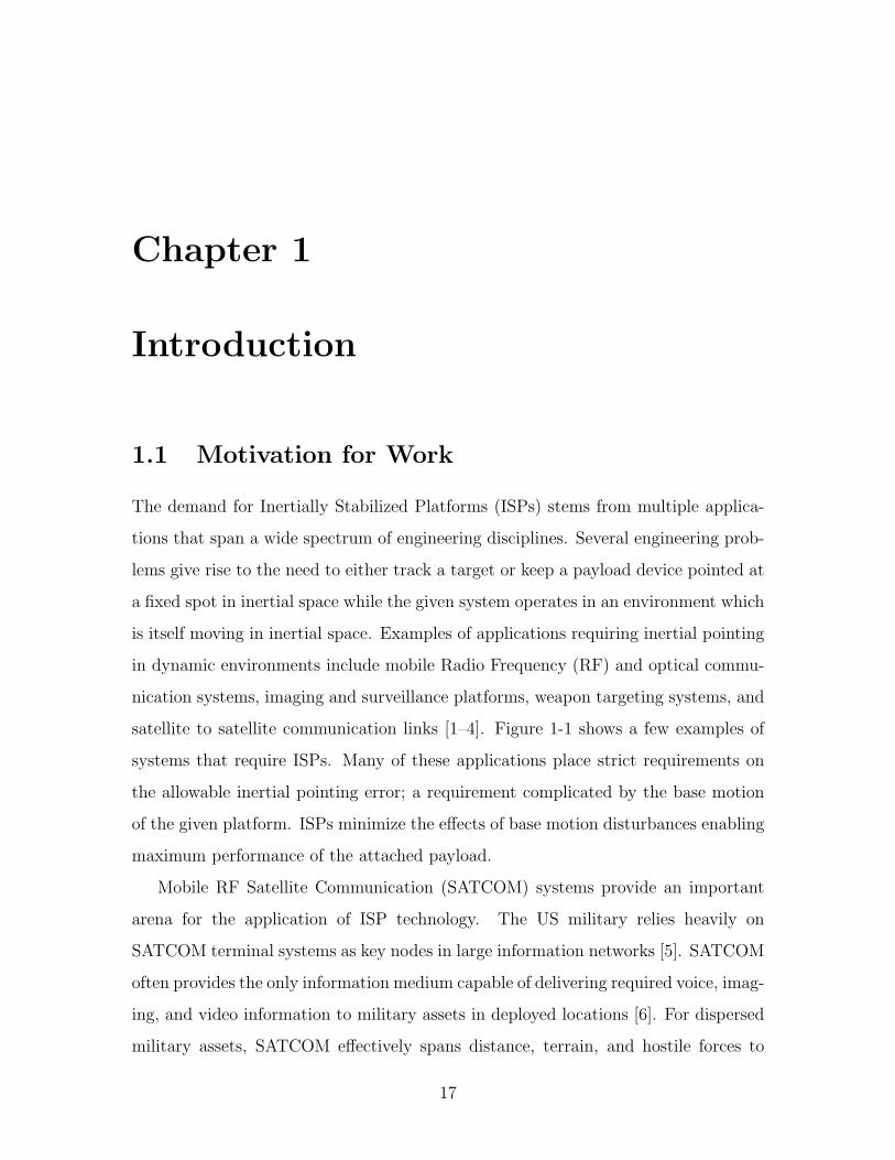
1.1 Motivation for Work
The demand for Inertially Stabilized Platforms (ISPs) stems from multiple applica-
tions that span a wide spectrum of engineering disciplines. Several engineering prob-
lems give rise to the need to either track a target or keep a payload device pointed at
a fixed spot in inertial space while the given system operates in an environment which
is itself moving in inertial space. Examples of applications requiring inertial pointing
in dynamic environments include mobile Radio Frequency (RF) and optical commu-
nication systems, imaging and surveillance platforms, weapon targeting systems, and
satellite to satellite communication links [1–4]. Figure 1-1 shows a few examples of
systems that require ISPs. Many of these applications place strict requirements on
the allowable inertial pointing error; a requirement complicated by the base motion
of the given platform. ISPs minimize the effects of base motion disturbances enabling
maximum performance of the attached payload.
Mobile RF Satellite Communication (SATCOM) systems provide an important
arena for the application of ISP technology. The US military relies heavily on
SATCOM terminal systems as key nodes in large information networks [5]. SATCOM
often provides the only information medium capable of delivering required voice, imag-
ing, and video information to military assets in deployed locations [6]. For dispersed
military assets, SATCOM effectively spans distance, terrain, and hostile forces to
17
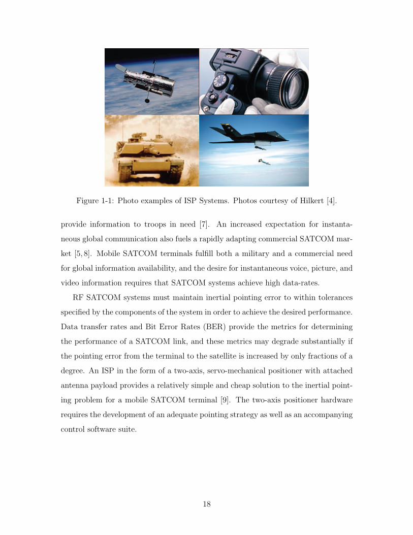
Figure 1-1: Photo examples of ISP Systems. Photos courtesy of Hilkert [4].
provide information to troops in need [7]. An increased expectation for instanta-
neous global communication also fuels a rapidly adapting commercial SATCOM mar-
ket [5, 8]. Mobile SATCOM terminals fulfill both a military and a commercial need
for global information availability, and the desire for instantaneous voice, picture, and
video information requires that SATCOM systems achieve high data-rates.
RF SATCOM systems must maintain inertial pointing error to within tolerances
specified by the components of the system in order to achieve the desired performance.
Data transfer rates and Bit Error Rates (BER) provide the metrics for determining
the performance of a SATCOM link, and these metrics may degrade substantially if
the pointing error from the terminal to the satellite is increased by only fractions of a
degree. An ISP in the form of a two-axis, servo-mechanical positioner with attached
antenna payload provides a relatively simple and cheap solution to the inertial point-
ing problem for a mobile SATCOM terminal [9]. The two-axis positioner hardware
requires the development of an adequate pointing strategy as well as an accompanying
control software suite.
18
1.2 Problem Statement
High data-rate RF SATCOM terminals require accurate spatial pointing of the an-
tenna payload. This thesis develops an inertial pointing strategy designed to meet the
pointing requirements for an airborne, Extremely High Frequency (EHF) SATCOM
terminal operating from a Boeing 707 aircraft owned and operated by MIT Lincoln
Laboratory. The terminal uses a two-axis, servo-mechanical Antenna Positioner Sys-
tem (APS) with a dish antenna payload. The pointing strategy developed for this
specific SATCOM application involves a hybrid open/closed loop approach. Open-
loop pointing in the context of this paper is defined as the pointing of an antenna at a
satellite without incorporating any RF signal strength measurements into the control
scheme. By contrast, closed-loop pointing methods do incorporate RF signal strength
feedback measurements in some fashion as a part of the pointing control strategy. It
is the goal of this thesis to recommend a solution to the antenna pointing problem
for the “EHF SATCOM on the 707” project, by:
1. Defining a nominal, two-axis APS and associated pointing requirements for
accomplishing an airborne EHF SATCOM mission
2. Developing an open-loop controller for the nominal APS using state-space and
optimal control techniques
3. Examining the performance of the open-loop pointing system through simula-
tion
4. Obtaining a model for the open-loop pointing error distributions in two orthog-
onal inertial coordinates
5. Examining ways that optimization programming strategies for nonlinear func-
tions may be applied to RF signal strength measurements to provide closed-loop
feedback in the form of refinements to the APS’s open-loop pointing commands
6. Comparing the performance of several optimization step-tracking algorithms, in
different configurations, on minimizing an antenna gain pattern cost function
19
7. Determining the overall feasibility of applying optimization methods to refine
open-loop pointing commands to minimize inertial pointing error
1.3 Contributions
This thesis makes the following contributions while accomplishing the objectives out-
lined in Section 1.2:
1. The thesis develops an open-loop pedestal controller, using optimal control tech-
niques, for a nominal two-axis, azimuth-elevation APS that mitigates the effects
of 707 aircraft motion and tracks input reference commands. The techniques
used to develop the open-loop controller for the nominal APS may be extended
to projects wishing to use two-axis pedestals on other mobile or stationary
SATCOM terminal systems.
2. A Simulink simulation is developed to test the performance of the open-loop
controller. The same simulation may be used in a slightly modified form to test
the open-loop pointing performance of similar APSs used on other SATCOM
terminals.
3. This thesis demonstrates the feasibility of using step-tracking algorithms to
accomplish closed-loop antenna pointing for a specific airborne SATCOM ap-
plication. The performance of several step-tracking algorithms is tested through
simulation, and the best performing algorithms are identified.
4. Simulations designed to test the robustness of the step-tracking algorithms are
also implemented to show that step-tracking provides a viable closed-loop point-
ing strategy even under harsher operating conditions than what may be ex-
pected for the nominal APS’s airborne EHF SATCOM mission. Although the
thesis develops step-tracking algorithms for use on a particular airborne termi-
nal system, the algorithms require only slight modifications to be used on other
SATCOM terminals.
20
5. This thesis demonstrates that accurate antenna pointing may be accomplished
by employing an open-loop pedestal controller in conjunction with a closed-loop
step-tracking algorithm. The hybrid open/closed-loop pointing strategy pre-
sented in this thesis may be implemented on future stationary and mobile SAT-
COM terminals. Hybrid pointing systems utilizing step-tracking procedures
require no additional hardware components to operate in a closed-loop fash-
ion and may, therefore, lead to the proliferation of simpler, more cost-effective
SATCOM terminal systems.
1.4 Thesis Overview
Chapter 2 of this thesis discusses the technologies available to accomplish a mobile
SATCOM mission. These technologies vary in complexity and cost, and Chapter 2
defines a nominal APS that will meet the pointing requirements for an airborne EHF
SATCOM mission with the simplest possible system. Thus, objective 1 from Section
1.2 is accomplished. Objectives 2 and 3 require the development of an open-loop
feedback controller for the nominal APS. Chapter 3 follows the development of the
feedback controller and develops linear and nonlinear open-loop pointing simulations.
Chapter 3 also develops a model for the statistical distributions of the components
of open-loop pointing error, satisfying objective number 4. The closed-loop point-
ing simulations implemented in Chapter 4 require an understanding of the behavior
of the open-loop pointing error. Chapter 4 develops step-tracking algorithms that
accomplish closed-loop antenna pointing. The step-tracking algorithms utilize non-
linear cost function optimization techniques, and several simulations are developed to
test the pointing performance of these algorithms in different configurations, accom-
plishing objectives 5 and 6. Finally, objective 7 is satisfied as the results of both the
open-loop pointing simulations and the closed-loop step-tracking simulations are dis-
cussed in Chapter 5 to determine the overall feasibility of a hybrid open/closed-loop
pointing strategy.
21

22

Chapter 2
Background and System
Architecture
Chapter Overview
Engineers may choose from multiple ISP configurations when determining the spatial
pointing approach that will meet the requirements of a given system. In mobile RF
SATCOM applications, the Antenna Positioner System (APS) serves as an ISP for
pointing an antenna payload at a target satellite to establish a communications link.
This chapter examines various configurations of APS hardware that could be used
to solve the inertial pointing problem in an RF SATCOM application. The sources
of error inherent in purely open-loop pointing strategies will be highlighted, and
the closed-loop pointing methods that may be implemented to compensate for these
shortcomings are discussed. Finally, this chapter identifies the hardware components
and pointing requirements for a nominal two-axis Antenna Positioner System that
closely models the actual APS used in the “EHF SATCOM on the 707 project.”
The development of a pointing strategy for this nominal APS will be the topic of
discussion in the following chapters.
23
2.1 APS Hardware Configurations
2.1.1 APS Components
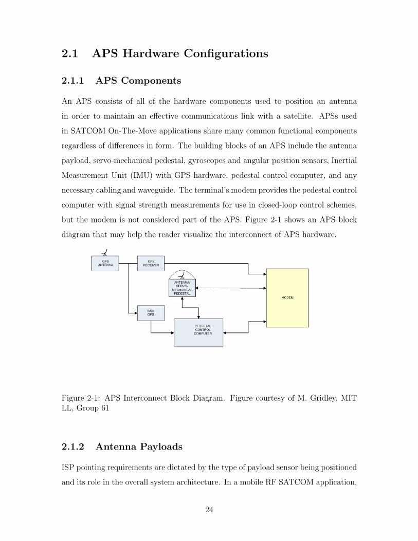
An APS consists of all of the hardware components used to position an antenna
in order to maintain an effective communications link with a satellite. APSs used
in SATCOM On-The-Move applications share many common functional components
regardless of differences in form. The building blocks of an APS include the antenna
payload, servo-mechanical pedestal, gyroscopes and angular position sensors, Inertial
Measurement Unit (IMU) with GPS hardware, pedestal control computer, and any
necessary cabling and waveguide. The terminal’s modem provides the pedestal control
computer with signal strength measurements for use in closed-loop control schemes,
but the modem is not considered part of the APS. Figure 2-1 shows an APS block
diagram that may help the reader visualize the interconnect of APS hardware.
Figure 2-1: APS Interconnect Block Diagram. Figure courtesy of M. Gridley, MITLL, Group 61
2.1.2 Antenna Payloads
ISP pointing requirements are dictated by the type of payload sensor being positioned
and its role in the overall system architecture. In a mobile RF SATCOM application,
24
the ISP’s payload is the antenna that the terminal uses to transmit to and receive
data from the satellite. In high-bandwidth SATCOM applications, antennas must be
directional and must exhibit high gain in accordance with the requirements of the
terminal system [9]. Antenna gain, measured in dB, is a measure of how well a par-
ticular antenna directs electromagnetic energy relative to an isotropic antenna, which
collects and emits electromagnetic energy equally in all directions. The gain of a direc-
tional antenna changes depending upon the incidence angle at which electromagnetic
waves intersect the antenna’s boresight, or direction of maximum gain. The variation
of gain with respect to pointing angle away from boresight forms an antenna’s gain
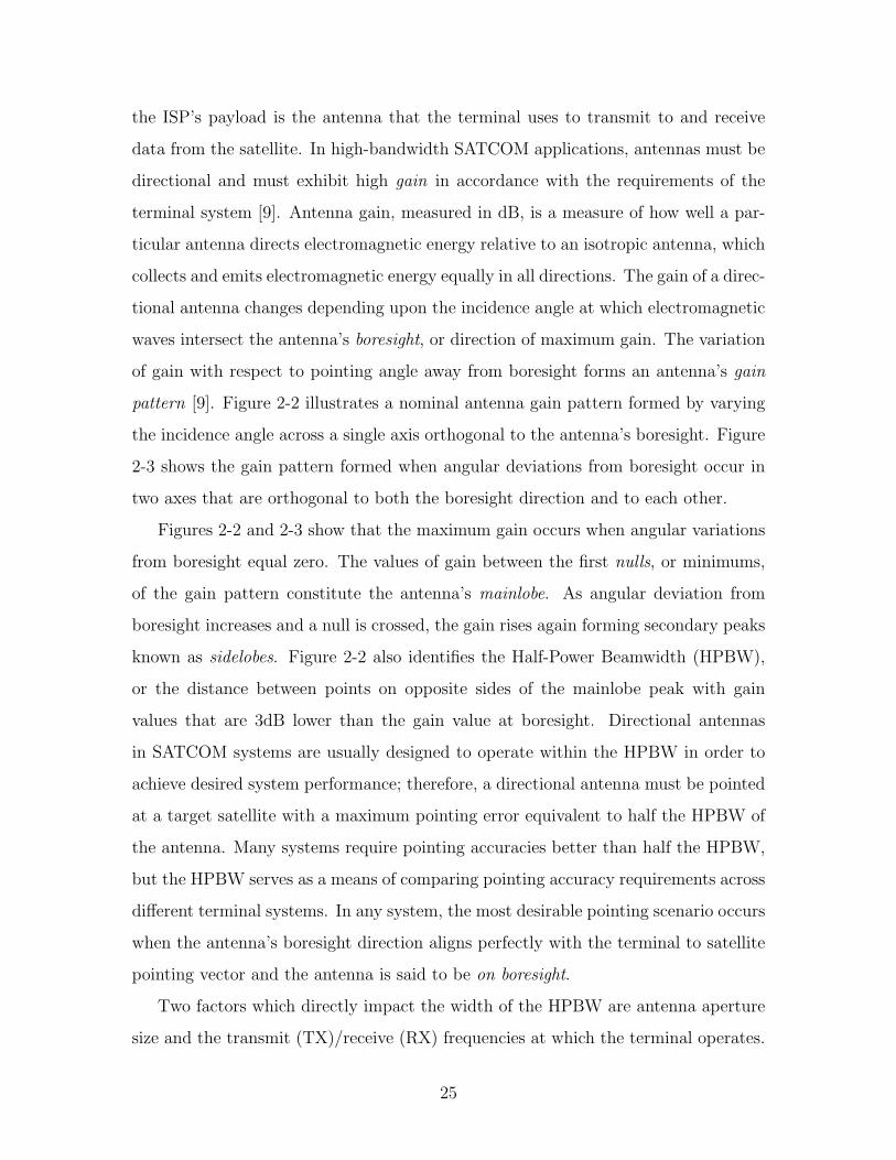
pattern [9]. Figure 2-2 illustrates a nominal antenna gain pattern formed by varying
the incidence angle across a single axis orthogonal to the antenna’s boresight. Figure
2-3 shows the gain pattern formed when angular deviations from boresight occur in
two axes that are orthogonal to both the boresight direction and to each other.
Figures 2-2 and 2-3 show that the maximum gain occurs when angular variations
from boresight equal zero. The values of gain between the first nulls, or minimums,
of the gain pattern constitute the antenna’s mainlobe. As angular deviation from
boresight increases and a null is crossed, the gain rises again forming secondary peaks
known as sidelobes. Figure 2-2 also identifies the Half-Power Beamwidth (HPBW),
or the distance between points on opposite sides of the mainlobe peak with gain
values that are 3dB lower than the gain value at boresight. Directional antennas
in SATCOM systems are usually designed to operate within the HPBW in order to
achieve desired system performance; therefore, a directional antenna must be pointed
at a target satellite with a maximum pointing error equivalent to half the HPBW of
the antenna. Many systems require pointing accuracies better than half the HPBW,
but the HPBW serves as a means of comparing pointing accuracy requirements across
different terminal systems. In any system, the most desirable pointing scenario occurs
when the antenna’s boresight direction aligns perfectly with the terminal to satellite
pointing vector and the antenna is said to be on boresight.
Two factors which directly impact the width of the HPBW are antenna aperture
size and the transmit (TX)/receive (RX) frequencies at which the terminal operates.
25
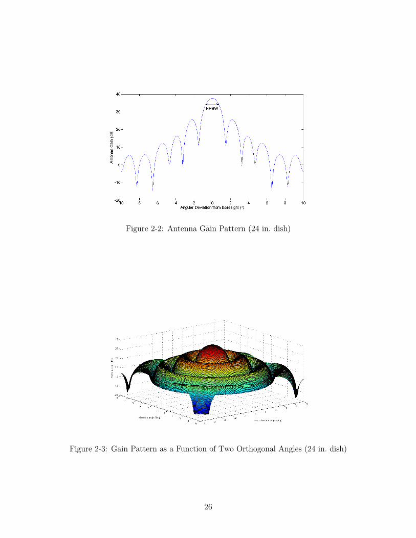
Figure 2-2: Antenna Gain Pattern (24 in. dish)
Figure 2-3: Gain Pattern as a Function of Two Orthogonal Angles (24 in. dish)
26
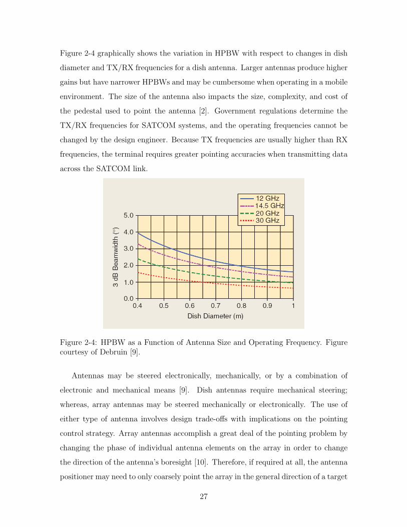
Figure 2-4 graphically shows the variation in HPBW with respect to changes in dish
diameter and TX/RX frequencies for a dish antenna. Larger antennas produce higher
gains but have narrower HPBWs and may be cumbersome when operating in a mobile
environment. The size of the antenna also impacts the size, complexity, and cost of
the pedestal used to point the antenna [2]. Government regulations determine the
TX/RX frequencies for SATCOM systems, and the operating frequencies cannot be
changed by the design engineer. Because TX frequencies are usually higher than RX
frequencies, the terminal requires greater pointing accuracies when transmitting data
across the SATCOM link.
Figure 2-4: HPBW as a Function of Antenna Size and Operating Frequency. Figurecourtesy of Debruin [9].
Antennas may be steered electronically, mechanically, or by a combination of
electronic and mechanical means [9]. Dish antennas require mechanical steering;
whereas, array antennas may be steered mechanically or electronically. The use of
either type of antenna involves design trade-offs with implications on the pointing
control strategy. Array antennas accomplish a great deal of the pointing problem by
changing the phase of individual antenna elements on the array in order to change
the direction of the antenna’s boresight [10]. Therefore, if required at all, the antenna
positioner may need to only coarsely point the array in the general direction of a target
27
or control pointing in only one axis. Due to their small size and low profile, array
antennas may integrate nicely with the structure of the given vehicle in a mobile
application. However, array antennas are expensive relative to dish antennas, and
they involve complex control algorithms for the electronic steering of the mainlobe [9].
As array antennas are electronically steered, the sidelobes in the gain pattern rise and
fall resulting in required software algorithms to suppress them to acceptable levels [10].
Dish antennas are cheaper but necessitate a servo-mechanical pedestal to point the
antenna in the desired direction. Integrating the RF waveguide with the particular
pedestal-antenna combination may also be challenging. For instance, the APS may
require a waveguide assembly to carry RF energy through the positioner by means
of rotary joints. For multi-axis pedestals, this task becomes more difficult and poses
additional design constraints. The use of simpler positioners or electronically steered
array antennas alleviates some of the design challenges of the RF waveguide system.
Another consideration for selecting the appropriate antenna for a mobile SATCOM
application is the method of antenna stabilization around the pointing vector. Dish
antennas exhibit an advantageous property known as mass stabilization [9]. Mass
stabilization is an extension of Newton’s first law which affirms that objects at rest
tend to remain at rest. Thus, although dish antennas require a servo-mechanical
pedestal to steer the antenna to different points in the sky, the positioner system
requires only relatively small amounts of motor torque to stabilize the antenna once
it is pointed. Mass stabilization is most beneficial for SATCOM applications where
target satellites are in geostationary orbits because the look angles from the terminal
to the satellite change very little under these circumstances. Mass-stabilized systems
still require motor control systems to provide motor torques to account for bearing
friction and other disturbance torques as well as to slew the antenna to different
positions in the sky.
Electronically steerable array antennas are, by nature, non-mass-stabilized [9].
If all pointing is done electronically, the lack of mass-stabilization does not pose a
significant problem because there is no mass to move in order to steer the antenna;
however, if some of the pointing is accomplished mechanically, torques proportional
28
to the size of the movable components are required from the pedestal motors. Iner-
tial Pointing Applications utilize other forms of stabilization including momentum-
wheel-stabilization, where rotating masses are used to provide inertially stable plat-
forms for mounting sensors. Momentum-wheel-stabilization techniques pose problems
for applications requiring sensors that change inertial pointing directions frequently,
and the spinning momentum-wheels could interfere with vehicle motion. Therefore,
momentum-wheel-stabilization techniques are not widely applied to terminals in SAT-
COM On-The-Move applications [4].
2.1.3 Pedestals and Sensors
The physical characteristics of servo-mechanical pedestals generally consist of a struc-
tural framework capable of rotational motion called a gimbal to which an assembly
of motors, bearings, gyroscopes, and payload devices are attached [4]. Pedestals used
in APSs may be classified as one-axis, two-axis, or multi-axis systems according to
the number of controllable axes present. Figure 2-5(a) illustrates gimbal devices for
typical two-axis pedestals. Multiple gimbals may sometimes be constructed to control
a sensor payload in the same axis. This set-up typically takes the form of a coarse
outer gimbal and accompanying motor configuration with an inner fine gimbal and
motor configuration as seen in Figure 2-5(b). The capabilities needed to maintain
adequate pointing of the payload in the region of inertial space relevant to the ap-
plication determines the number of required controllable axes for a pedestal system.
In RF SATCOM applications, only the inertial axes orthogonal to the pointing
vector from the antenna to the target satellite need to be controlled by the APS.
Motion in the antenna’s roll axis is not relevant to the pointing problem due to the
symmetric nature of the gain pattern. Two-axis servo-mechanical pedestals using an
azimuth-elevation gimbal configuration are commonplace in SATCOM applications
because, together, the two axes provide a complete hemispherical field-of-regard [9].
Figure 2-6 shows the two-axis pedestal and antenna used on the “EHF SATCOM on
the 707 Project.” The azimuth-elevation positioner provides an adequate solution for
29
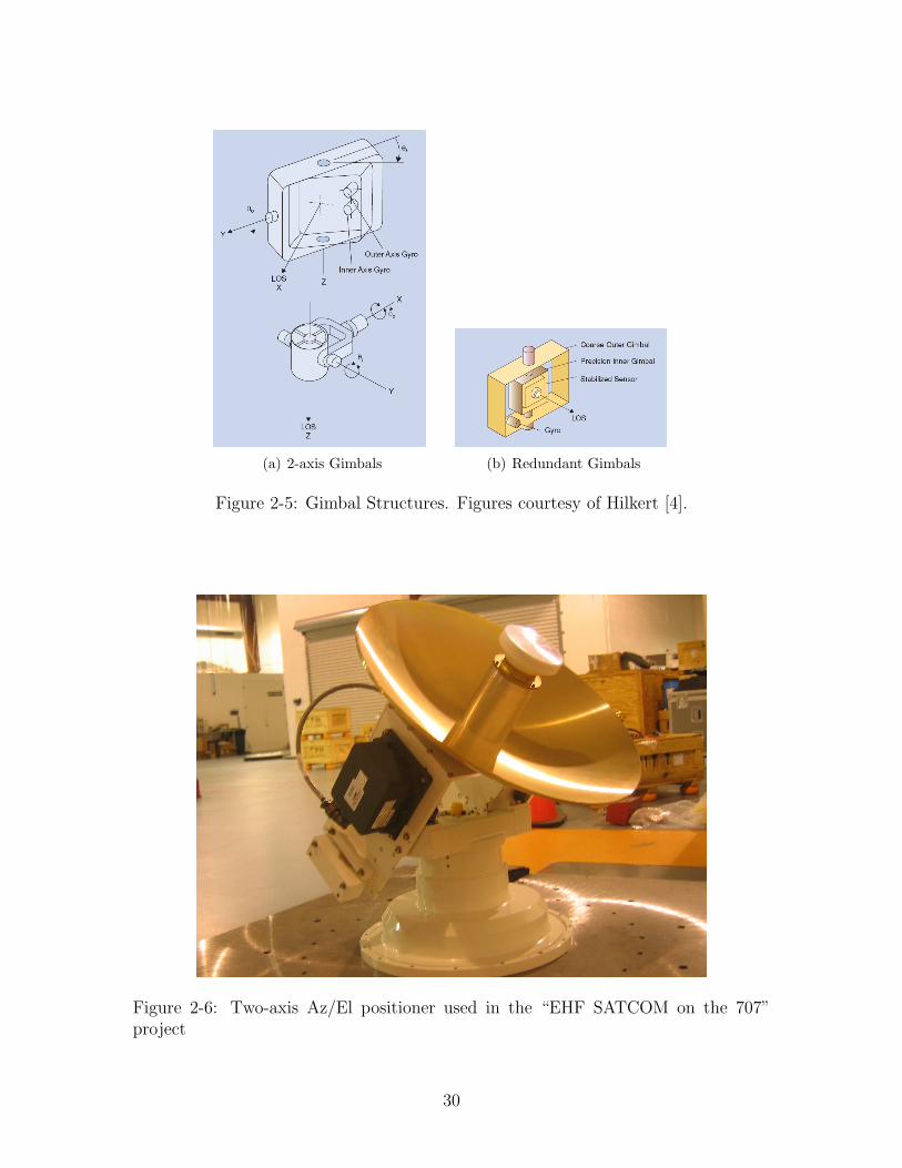
(a) 2-axis Gimbals (b) Redundant Gimbals
Figure 2-5: Gimbal Structures. Figures courtesy of Hilkert [4].
Figure 2-6: Two-axis Az/El positioner used in the “EHF SATCOM on the 707”project
30
antenna pointing under many conditions. Additional steerable axes may be added to
the basic two-axis configuration to achieve added base motion disturbance rejection,
increase the field-of-regard of the pedestal, and to eliminate singularities that can
result from simple two-axis configurations [4].
The major concern with operating a two-axis, azimuth-elevation antenna posi-
tioner occurs when the application requires pointing in the keyhole region. The key-
hole region is loosely defined as pedestal operation at local elevation angles greater
than 80 [9]. During tracking, the azimuth motor attempts to correct for vehicle mo-
tions that occur in the roll axis of the pedestal’s base. The pedestal base roll axis is
the same as vehicle roll when the pedestal’s azimuth gimbal is aligned with the front
or back of the vehicle. Angular motion about the pedestal base roll axis corresponds
to rotations in the vehicle’s pitch direction when the pedestal’s azimuth gimbal is
pointed to either side of the vehicle. Vehicle motion in the roll axis of the pedestal’s
base becomes more difficult to account for with a two-axis pedestal as elevation angles
approach the keyhole region and a singularity known as gimbal lock results [4]. The
required azimuth motor velocity varies with elevation angle, el, according to
azd = − tan(el)P ′Base −R′Base (2.1)
where azd is the azimuth motor velocity required to maintain fixed inertial pointing,
P ′Base is the vehicle motion resolved in the roll axis of the pedestal’s base, and R′Base is
the vehicle motion resolved in the yaw axis of the pedestal’s base (Equations (A.17)
and (A.18)). Equation (2.1) clearly shows how an infinite azimuth motor velocity
is required at an elevation angle of 90, and the azimuth motor eventually lacks the
required torque to keep the antenna pointed correctly as elevation angles enter the
keyhole region. Several different configurations for multi-axis pedestals exist, but
most are designed explicitly to eliminate the gimbal lock singularity in the keyhole
region. The reader is referred to the literature for more information on multi-axis
pedestals [9,11]. Despite the advantages that multi-axis pedestals maintain over two-
axis configurations in avoiding gimbal lock, all else being equal, two-axis pedestals
31

are generally stiffer, cheaper, more compact, and less complex than their multi-axis
counterparts [9]. Therefore, the design engineer may find it beneficial to use a two-axis
pedestal whenever possible.
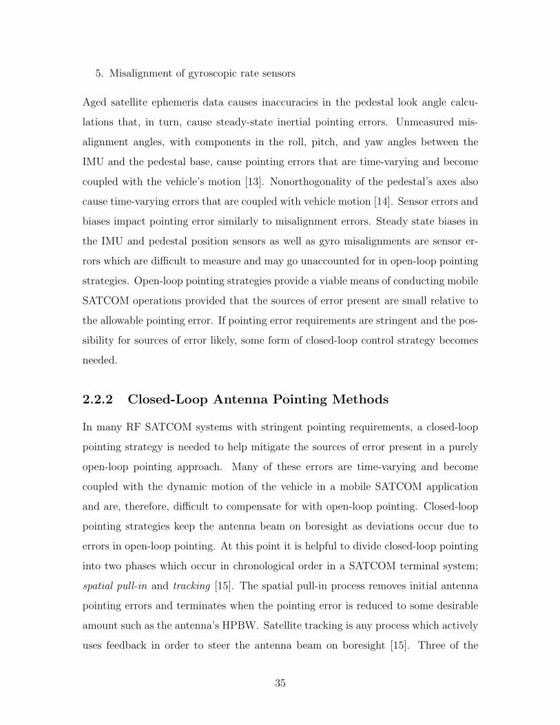
Angular position and rate sensors are typically installed in locations of interest on
the pedestal in order to facilitate feedback for the pedestal controller. Position sensors
may take the form of encoders or resolvers and are installed in the movable axes of
the pedestal. Angular position sensors exhibit different degrees of accuracy dependent
upon their complexity and cost. Gyroscopic sensors measure angular rates about the
axes of interest and vary greatly in terms of cost and performance. Figure 2-7 shows
the relative accuracies, in terms of scale factor and bias stabilities, for a number of
different types of gyroscopic sensors. Figure 2-7 also maps specific applications to
the different types of gyroscopic sensors that may be used in the applications. This
mapping provides a holistic comparison of the quality of gyroscopic sensors. Inertial
Measurement Units contain gyroscopes and accelerometers and measure the inertial
states of the vehicle upon which the pedestal is mounted. Because vehicles are not
true rigid bodies, they exhibit varying degrees of flexure necessitating placement of
the IMU in a location very near or on the base of the pedestal in order to obtain
accurate measurements of the vehicle’s motion. The accuracy and alignment of all
sensors impacts the pointing performance of the APS.
2.1.4 APS Design Requirements
The specific SATCOM mission determines the requirements that an APS must fulfill.
The design engineer must select the appropriate APS hardware such that all require-
ments of the system are met, and the desired inertial pointing accuracy is achieved.
The APS must meet specified size and weight requirements which are particularly
stringent for mobile terminal systems [2]. The mass and inertia of the antenna pay-
load determines the size and weight of the servo-mechanical pedestal. When size and
weight are limiting factors in design, the attainable pointing accuracy may become
a design tradeoff. For mobile terminals using mechanically steered antennas, the dy-
namics of the operating environment determine velocity and acceleration requirements
32
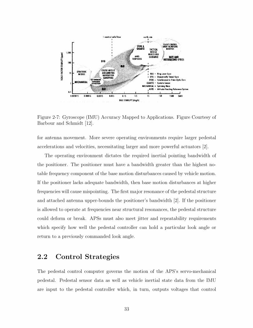
Figure 2-7: Gyroscope (IMU) Accuracy Mapped to Applications. Figure Courtesy ofBarbour and Schmidt [12].
for antenna movement. More severe operating environments require larger pedestal
accelerations and velocities, necessitating larger and more powerful actuators [2].
The operating environment dictates the required inertial pointing bandwidth of
the positioner. The positioner must have a bandwidth greater than the highest no-
table frequency component of the base motion disturbances caused by vehicle motion.
If the positioner lacks adequate bandwidth, then base motion disturbances at higher
frequencies will cause mispointing. The first major resonance of the pedestal structure
and attached antenna upper-bounds the positioner’s bandwidth [2]. If the positioner
is allowed to operate at frequencies near structural resonances, the pedestal structure
could deform or break. APSs must also meet jitter and repeatability requirements
which specify how well the pedestal controller can hold a particular look angle or
return to a previously commanded look angle.
2.2 Control Strategies
The pedestal control computer governs the motion of the APS’s servo-mechanical
pedestal. Pedestal sensor data as well as vehicle inertial state data from the IMU
are input to the pedestal controller which, in turn, outputs voltages that control
33
the DC motor circuits in the pedestal. The pedestal controller may also interface
with the terminal’s modem to receive RF signal strength measurements for use in
closed-loop pointing control strategies. The voltage outputs to the pedestal motors
are governed by feedback control loops that are implemented as a part of an overall
pointing strategy which may be open or closed-loop.
2.2.1 Open-loop Pointing and Sources of Error
Open-loop pointing techniques implemented in mobile SATCOM systems involve sim-
ilar pedestal control issues as those encountered in other applications such as fixed
ground station SATCOM, aerial surveillance, and weapon systems targeting [9]. The
goal of the controller in an open-loop configuration is to negate the effects of vehicle
base motion disturbances while simultaneously following an input reference command.
APSs used in mobile SATCOM applications continuously obtain measurements of the
vehicle’s inertial states and calculate desired look angles to the target satellite in the
pedestal’s local reference frame. These look angles are fed as reference commands to a
feedback control loop which steers the pedestal to the desired location. The kinematic
equations and coordinate transformations which govern the look angle calculations
for a two-axis APS are presented in Appendix A. The open-loop controller accounts
for base motion disturbances by quickly updating the look angle reference commands,
by direct feedback of the antenna’s inertial states to the feedback controller, or by a
combination of the two approaches.
Open-loop pointing strategies involve sources of error which may lead to mispoint-
ing of the antenna in inertial space. Notable sources of error which may not be taken
into account in open-loop pointing schemes include:
1. Aged satellite ephemeris data
2. Unmeasured IMU misalignment angles
3. Nonorthogonality of pedestal axes
4. Steady-state biases in pedestal position sensors and the IMU
34
5. Misalignment of gyroscopic rate sensors
Aged satellite ephemeris data causes inaccuracies in the pedestal look angle calcu-
lations that, in turn, cause steady-state inertial pointing errors. Unmeasured mis-
alignment angles, with components in the roll, pitch, and yaw angles between the
IMU and the pedestal base, cause pointing errors that are time-varying and become
coupled with the vehicle’s motion [13]. Nonorthogonality of the pedestal’s axes also
cause time-varying errors that are coupled with vehicle motion [14]. Sensor errors and
biases impact pointing error similarly to misalignment errors. Steady state biases in
the IMU and pedestal position sensors as well as gyro misalignments are sensor er-
rors which are difficult to measure and may go unaccounted for in open-loop pointing
strategies. Open-loop pointing strategies provide a viable means of conducting mobile
SATCOM operations provided that the sources of error present are small relative to
the allowable pointing error. If pointing error requirements are stringent and the pos-
sibility for sources of error likely, some form of closed-loop control strategy becomes
needed.
2.2.2 Closed-Loop Antenna Pointing Methods
In many RF SATCOM systems with stringent pointing requirements, a closed-loop
pointing strategy is needed to help mitigate the sources of error present in a purely
open-loop pointing approach. Many of these errors are time-varying and become
coupled with the dynamic motion of the vehicle in a mobile SATCOM application
and are, therefore, difficult to compensate for with open-loop pointing. Closed-loop
pointing strategies keep the antenna beam on boresight as deviations occur due to
errors in open-loop pointing. At this point it is helpful to divide closed-loop pointing
into two phases which occur in chronological order in a SATCOM terminal system;
spatial pull-in and tracking [15]. The spatial pull-in process removes initial antenna
pointing errors and terminates when the pointing error is reduced to some desirable
amount such as the antenna’s HPBW. Satellite tracking is any process which actively
uses feedback in order to steer the antenna beam on boresight [15]. Three of the
35
most prevalent closed-loop pointing techniques are monopulse, conical scan, and step-
tracking [16].
Monopulse tracking involves the use of additional hardware, in the form of one or
more antennas in addition to the main antenna, which measure the signal strength of
the communications link. By comparing the signal levels received in the monopulse
antennas, the main antenna may be steered in the appropriate direction to eliminate
pointing errors [17, 18]. Because the mispointing feedback is nearly continuous, con-
trollers can be designed to close the loop around the pointing error feedback metric.
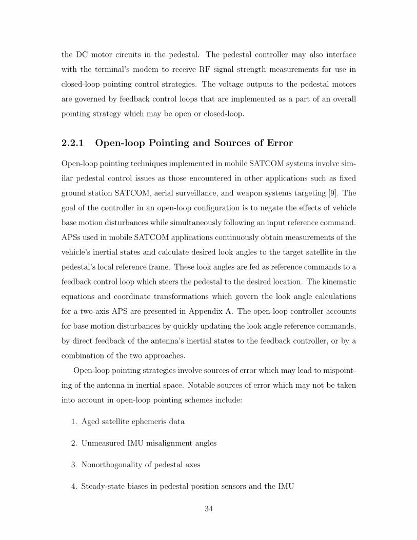
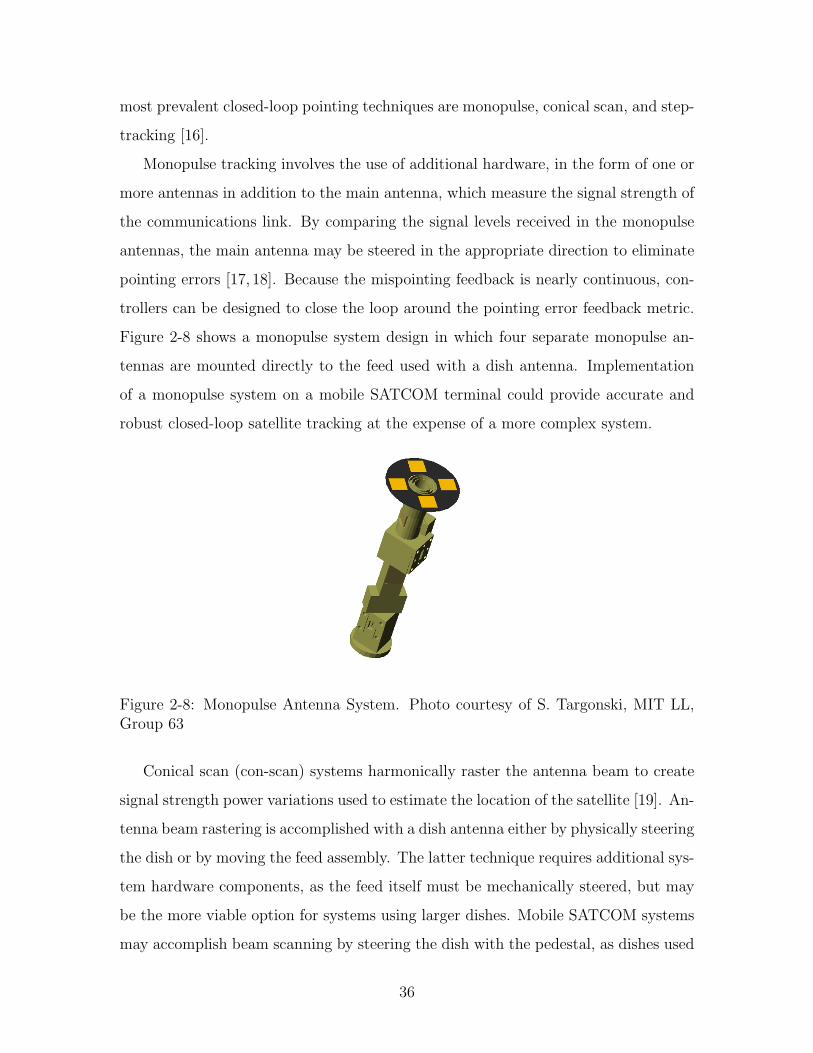
Figure 2-8 shows a monopulse system design in which four separate monopulse an-
tennas are mounted directly to the feed used with a dish antenna. Implementation
of a monopulse system on a mobile SATCOM terminal could provide accurate and
robust closed-loop satellite tracking at the expense of a more complex system.
Figure 2-8: Monopulse Antenna System. Photo courtesy of S. Targonski, MIT LL,Group 63
Conical scan (con-scan) systems harmonically raster the antenna beam to create
signal strength power variations used to estimate the location of the satellite [19]. An-
tenna beam rastering is accomplished with a dish antenna either by physically steering
the dish or by moving the feed assembly. The latter technique requires additional sys-
tem hardware components, as the feed itself must be mechanically steered, but may
be the more viable option for systems using larger dishes. Mobile SATCOM systems
may accomplish beam scanning by steering the dish with the pedestal, as dishes used
36
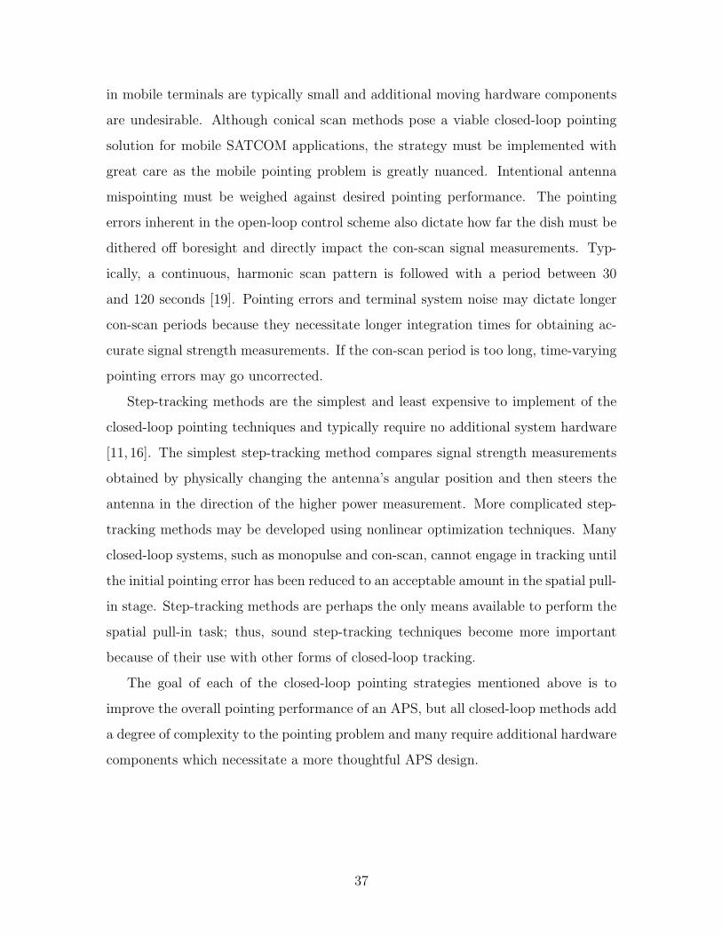
in mobile terminals are typically small and additional moving hardware components
are undesirable. Although conical scan methods pose a viable closed-loop pointing
solution for mobile SATCOM applications, the strategy must be implemented with
great care as the mobile pointing problem is greatly nuanced. Intentional antenna
mispointing must be weighed against desired pointing performance. The pointing
errors inherent in the open-loop control scheme also dictate how far the dish must be
dithered off boresight and directly impact the con-scan signal measurements. Typ-
ically, a continuous, harmonic scan pattern is followed with a period between 30
and 120 seconds [19]. Pointing errors and terminal system noise may dictate longer
con-scan periods because they necessitate longer integration times for obtaining ac-
curate signal strength measurements. If the con-scan period is too long, time-varying
pointing errors may go uncorrected.
Step-tracking methods are the simplest and least expensive to implement of the
closed-loop pointing techniques and typically require no additional system hardware
[11, 16]. The simplest step-tracking method compares signal strength measurements
obtained by physically changing the antenna’s angular position and then steers the
antenna in the direction of the higher power measurement. More complicated step-
tracking methods may be developed using nonlinear optimization techniques. Many
closed-loop systems, such as monopulse and con-scan, cannot engage in tracking until
the initial pointing error has been reduced to an acceptable amount in the spatial pull-
in stage. Step-tracking methods are perhaps the only means available to perform the
spatial pull-in task; thus, sound step-tracking techniques become more important
because of their use with other forms of closed-loop tracking.
The goal of each of the closed-loop pointing strategies mentioned above is to
improve the overall pointing performance of an APS, but all closed-loop methods add
a degree of complexity to the pointing problem and many require additional hardware
components which necessitate a more thoughtful APS design.
37
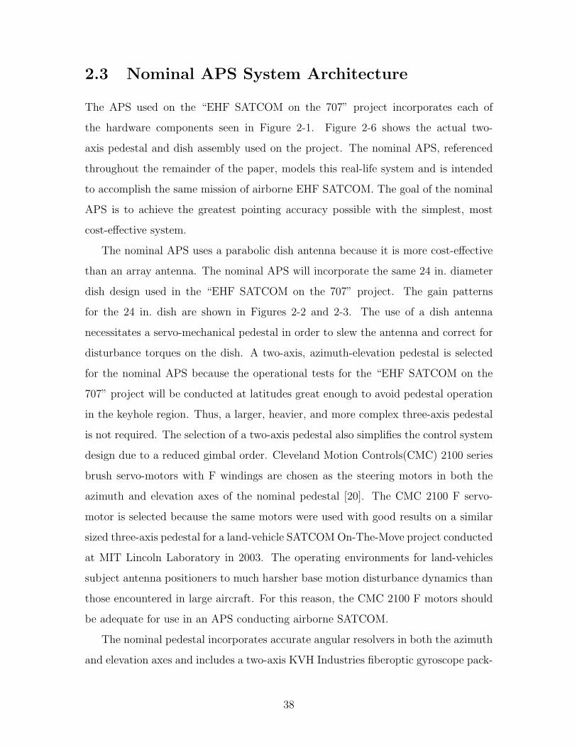
2.3 Nominal APS System Architecture
The APS used on the “EHF SATCOM on the 707” project incorporates each of
the hardware components seen in Figure 2-1. Figure 2-6 shows the actual two-
axis pedestal and dish assembly used on the project. The nominal APS, referenced
throughout the remainder of the paper, models this real-life system and is intended
to accomplish the same mission of airborne EHF SATCOM. The goal of the nominal
APS is to achieve the greatest pointing accuracy possible with the simplest, most
cost-effective system.
The nominal APS uses a parabolic dish antenna because it is more cost-effective
than an array antenna. The nominal APS will incorporate the same 24 in. diameter
dish design used in the “EHF SATCOM on the 707” project. The gain patterns
for the 24 in. dish are shown in Figures 2-2 and 2-3. The use of a dish antenna
necessitates a servo-mechanical pedestal in order to slew the antenna and correct for
disturbance torques on the dish. A two-axis, azimuth-elevation pedestal is selected
for the nominal APS because the operational tests for the “EHF SATCOM on the
707” project will be conducted at latitudes great enough to avoid pedestal operation
in the keyhole region. Thus, a larger, heavier, and more complex three-axis pedestal
is not required. The selection of a two-axis pedestal also simplifies the control system
design due to a reduced gimbal order. Cleveland Motion Controls(CMC) 2100 series
brush servo-motors with F windings are chosen as the steering motors in both the
azimuth and elevation axes of the nominal pedestal [20]. The CMC 2100 F servo-
motor is selected because the same motors were used with good results on a similar
sized three-axis pedestal for a land-vehicle SATCOM On-The-Move project conducted
at MIT Lincoln Laboratory in 2003. The operating environments for land-vehicles
subject antenna positioners to much harsher base motion disturbance dynamics than
those encountered in large aircraft. For this reason, the CMC 2100 F motors should
be adequate for use in an APS conducting airborne SATCOM.
The nominal pedestal incorporates accurate angular resolvers in both the azimuth
and elevation axes and includes a two-axis KVH Industries fiberoptic gyroscope pack-
38
age mounted to the elevation gimbal in order to measure the inertial rates of the dish
antenna in the pitch and yaw axes [21]. The fiberoptic gyroscopes used are employed
in munitions guidance systems and should provide adequate measurements in spatial
tracking applications (Figure 2-7). The project uses a C-MIGITS IMU system to
measure the inertial states of the 707 aircraft at the location where the pedestal is
mounted. The C-MIGITS is a navigation-grade IMU that is also frequently used in
munitions guidance applications [22].
The nominal APS must incorporate a pedestal feedback controller which will limit
inertial pointing error to within 0.1 (3-σ) of boresight in an open-loop pointing
simulation. The gain patterns for the 24 in. dish shown in Figures 2-2 and 2-3
illustrate that an inertial pointing error of 0.1 would have a negligible impact on the
quality of the SATCOM link. Because of the sources of error identified in Section
2.2.1, the desired pointing requirement of 0.1 may not be achievable while operating
in a purely open-loop fashion. For this reason, the nominal APS requires inertial
pointing to within 0.25 of boresight or better in a closed-loop pointing simulation.
Inertial pointing error of 0.25 corresponds to a 0.4 dB loss in signal strength and
would have very little impact on the overall performance of the SATCOM link (Figure
2-2). With the hardware and pointing requirements for the nominal APS now defined,
the open-loop portion of the hybrid pointing control strategy may be developed.
39

40
Chapter 3
Open-Loop Controller
Development
Chapter Overview
Open-loop pointing strategies necessitate a feedback controller for the mechanical
pedestal used to position the antenna payload. In this chapter, a Linear Quadratic
Gaussian (LQG) controller will be developed, based on the nominal two-axis APS
defined in the previous chapter, to effectively control the pedestal’s azimuth and
elevation DC servo-motors. For typical flight profiles, this controller will be able to
reduce the effects of base motion disturbances caused by aircraft motion and keep the
antenna dish inertially pointed at a target satellite. The controller will operate in a
closed-loop fashion, obtaining feedback from the inertial states of the antenna, but
because RF signal strength measurements are not introduced into the control scheme,
the resulting controller is classified as open-loop in the context of the definitions
from Section 1.2. After the feedback controller is developed, and the performance is
simulated, the statistical distributions for the components of inertial pointing error
will be modeled for use in closed-loop pointing simulations developed in the next
chapter.
41
3.1 Equations of Motion
3.1.1 Response Side
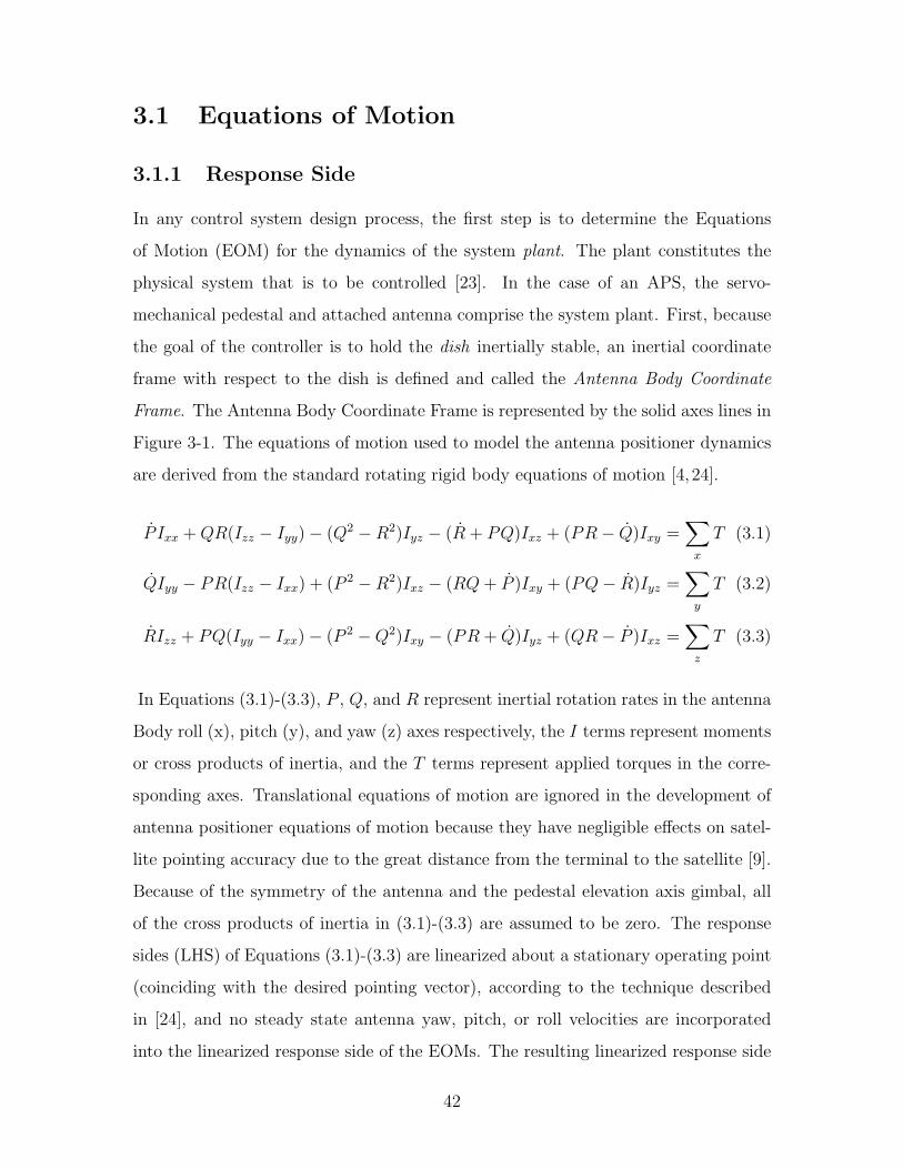
In any control system design process, the first step is to determine the Equations
of Motion (EOM) for the dynamics of the system plant. The plant constitutes the
physical system that is to be controlled [23]. In the case of an APS, the servo-
mechanical pedestal and attached antenna comprise the system plant. First, because
the goal of the controller is to hold the dish inertially stable, an inertial coordinate
frame with respect to the dish is defined and called the Antenna Body Coordinate
Frame. The Antenna Body Coordinate Frame is represented by the solid axes lines in
Figure 3-1. The equations of motion used to model the antenna positioner dynamics
are derived from the standard rotating rigid body equations of motion [4, 24].
P Ixx +QR(Izz − Iyy)− (Q2 −R2)Iyz − (R + PQ)Ixz + (PR− Q)Ixy =∑x
T (3.1)
QIyy − PR(Izz − Ixx) + (P 2 −R2)Ixz − (RQ+ P )Ixy + (PQ− R)Iyz =∑y
T (3.2)
RIzz + PQ(Iyy − Ixx)− (P 2 −Q2)Ixy − (PR + Q)Iyz + (QR− P )Ixz =∑z
T (3.3)
In Equations (3.1)-(3.3), P , Q, and R represent inertial rotation rates in the antenna
Body roll (x), pitch (y), and yaw (z) axes respectively, the I terms represent moments
or cross products of inertia, and the T terms represent applied torques in the corre-
sponding axes. Translational equations of motion are ignored in the development of
antenna positioner equations of motion because they have negligible effects on satel-
lite pointing accuracy due to the great distance from the terminal to the satellite [9].
Because of the symmetry of the antenna and the pedestal elevation axis gimbal, all
of the cross products of inertia in (3.1)-(3.3) are assumed to be zero. The response
sides (LHS) of Equations (3.1)-(3.3) are linearized about a stationary operating point
(coinciding with the desired pointing vector), according to the technique described
in [24], and no steady state antenna yaw, pitch, or roll velocities are incorporated
into the linearized response side of the EOMs. The resulting linearized response side
42
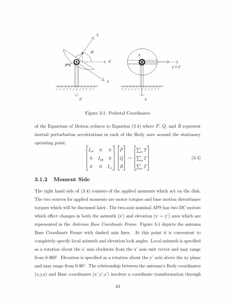
Figure 3-1: Pedestal Coordinates
of the Equations of Motion reduces to Equation (3.4) where P , Q, and R represent
inertial perturbation accelerations in each of the Body axes around the stationary
operating point. Ixx 0 0
0 Iyy 0
0 0 Izz
P
Q
R
=
∑
x T∑y T∑z T
(3.4)
3.1.2 Moment Side
The right hand side of (3.4) consists of the applied moments which act on the dish.
The two sources for applied moments are motor torques and base motion disturbance
torques which will be discussed later. The two-axis nominal APS has two DC motors
which effect changes in both the azimuth (z’) and elevation (y = y’) axes which are
represented in the Antenna Base Coordinate Frame. Figure 3-1 depicts the antenna
Base Coordinate Frame with dashed axis lines. At this point it is convenient to
completely specify local azimuth and elevation look angles. Local azimuth is specified
as a rotation about the z’ axis clockwise from the x’ axis unit vector and may range
from 0-360. Elevation is specified as a rotation about the y’ axis above the xy plane
and may range from 0-90. The relationship between the antenna’s Body coordinates
(x,y,z) and Base coordinates (x’,y’,z’) involves a coordinate transformation through
43
a negative elevation angle (3.5).
x′
y′
z′
Base
=
cos(el) 0 sin(el)
0 1 0
− sin(el) 0 cos(el)
x
y
z
Body
(3.5)
Because the azimuth motor acts in the z’ axis, its applied torque enters nonlinearly
into the Body x and z axes due to a coordinate transformation; whereas, the elevation
motor applies torque directly to the Body y axis (3.6).
∑
x Tmotor∑y Tmotor∑z Tmotor
=
− sin(el)Taz
Tel
cos(el)Taz
(3.6)
For a DC motor, applied torques (T ) are proportional to the current in the arma-
ture circuit, ia (3.7). In Equation (3.7), Km is the motor constant for the particular
DC motor. The armature current is governed by a differential equation that accounts
for armature inductance (La) and resistance (Ra), back emf voltage (eb), and applied
armature voltage (ea) (3.8). Back emf voltage results from the rotating armature and
is proportional to the angular velocity (θ1) of the motor shaft by a constant, (Kb),
which is approximately the reciprocal of Km (3.9). The applied armature voltage is
the value eventually determined by the feedback controller to effect the desired motor
torque [23].
T = Kmia (3.7)
ea = Ladiadt
+Raia + eb (3.8)
eb = Kbθ1 (3.9)
If armature inductance is neglected, which is often the case due to its small value, then
the applied motor torques for the azimuth and elevation motors may be represented
44
as in (3.10) and (3.11).
Taz =Kmaz
Raaz
eaaz −KmazKbaz
Raaz
[− sin(el)θroll + cos(el)θyaw] (3.10)
Tel =Kmel
Rael
eael −KmelKbel
Rael
θpitch (3.11)
In Equations (3.10)-(3.11) the angular velocities of the motor shafts, represented in
the Base coordinate frame, are expressed in terms of the angular velocities of the dish
with respect to the aircraft in the Body frame (3.12).
θroll
θpitch
θyaw
Base
=
cos(el) 0 − sin(el)
0 1 0
sin(el) 0 cos(el)
0
θel
θaz
Body
(3.12)
The nominal APS incorporates a gear train to magnify the applied steering torques
on the dish without using larger motors. The gear ratio (ng) is defined as the ratio
of the radius of the smaller gear (r1), mounted to the motor shaft, to the radius of
the larger gear (r2) that is mounted to the output shaft [23]. The following relation-
ship relating the angular velocities of the motor shaft and the output shaft may be
determined [23]:
θ2
θ1
=r1
r2
= ng (3.13)
where θ1 is the angular velocity of the motor shaft and θ2 is the angular velocity of
the output shaft. Using Equation (3.13) and the fact that the inertias of the motor
shafts are very small compared to the inertias of the antenna and elevation gimbal
assembly, Equations (3.4), (3.6), (3.10), and (3.11) may be combined, incorporating
the gear train, to yield (3.14).
45
Ixx 0 0
0 Iyy 0
0 0 Izz
P
Q
R
=
− KmazngRaaz
eaaz sin(el)− KmazKbazn2gRaaz
sin2(el)θroll
+KmazKbazn2gRaaz
sin(el) cos(el)θyaw +∑
x Tdisturbance
KmelngRael
eael −KmelKbeln2gRael
θpitch +∑
y Tdisturbance
KmazngRaaz
eaaz cos(el) +KmazKbazn2gRaaz
sin(el) cos(el)θroll
−KmazKbazn2gRaaz
cos2(el)θyaw +∑
z Tdisturbance
(3.14)
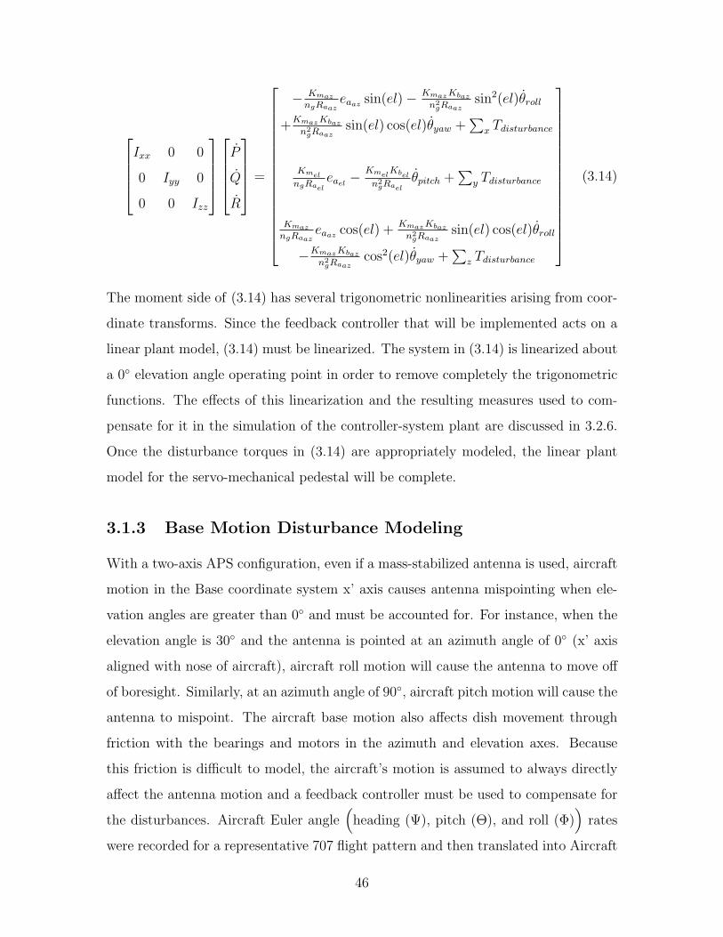
The moment side of (3.14) has several trigonometric nonlinearities arising from coor-
dinate transforms. Since the feedback controller that will be implemented acts on a
linear plant model, (3.14) must be linearized. The system in (3.14) is linearized about
a 0 elevation angle operating point in order to remove completely the trigonometric
functions. The effects of this linearization and the resulting measures used to com-
pensate for it in the simulation of the controller-system plant are discussed in 3.2.6.
Once the disturbance torques in (3.14) are appropriately modeled, the linear plant
model for the servo-mechanical pedestal will be complete.
3.1.3 Base Motion Disturbance Modeling
With a two-axis APS configuration, even if a mass-stabilized antenna is used, aircraft
motion in the Base coordinate system x’ axis causes antenna mispointing when ele-
vation angles are greater than 0 and must be accounted for. For instance, when the
elevation angle is 30 and the antenna is pointed at an azimuth angle of 0 (x’ axis
aligned with nose of aircraft), aircraft roll motion will cause the antenna to move off
of boresight. Similarly, at an azimuth angle of 90, aircraft pitch motion will cause the
antenna to mispoint. The aircraft base motion also affects dish movement through
friction with the bearings and motors in the azimuth and elevation axes. Because
this friction is difficult to model, the aircraft’s motion is assumed to always directly
affect the antenna motion and a feedback controller must be used to compensate for
the disturbances. Aircraft Euler angle(
heading (Ψ), pitch (Θ), and roll (Φ))
rates
were recorded for a representative 707 flight pattern and then translated into Aircraft
46
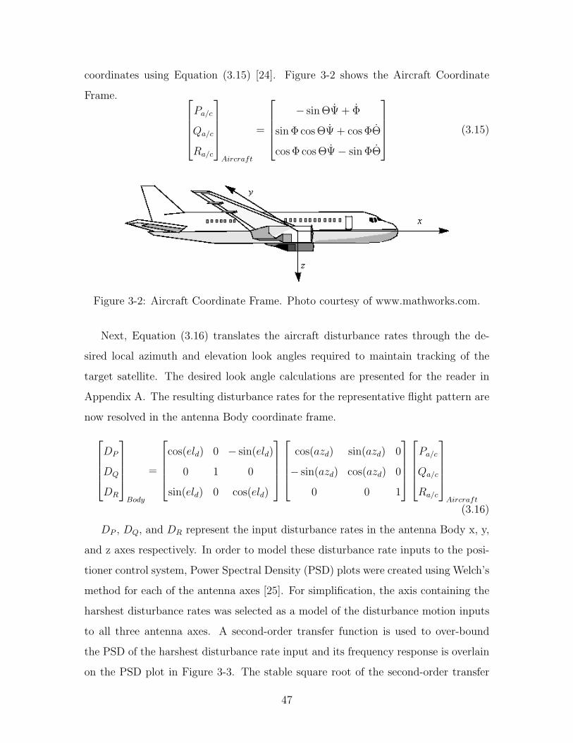
coordinates using Equation (3.15) [24]. Figure 3-2 shows the Aircraft Coordinate
Frame. Pa/c
Qa/c
Ra/c
Aircraft
=
− sin ΘΨ + Φ
sin Φ cos ΘΨ + cos ΦΘ
cos Φ cos ΘΨ− sin ΦΘ
(3.15)
Figure 3-2: Aircraft Coordinate Frame. Photo courtesy of www.mathworks.com.
Next, Equation (3.16) translates the aircraft disturbance rates through the de-
sired local azimuth and elevation look angles required to maintain tracking of the
target satellite. The desired look angle calculations are presented for the reader in
Appendix A. The resulting disturbance rates for the representative flight pattern are
now resolved in the antenna Body coordinate frame.DP
DQ
DR
Body
=
cos(eld) 0 − sin(eld)
0 1 0
sin(eld) 0 cos(eld)
cos(azd) sin(azd) 0
− sin(azd) cos(azd) 0
0 0 1
Pa/c
Qa/c
Ra/c
Aircraft
(3.16)
DP , DQ, and DR represent the input disturbance rates in the antenna Body x, y,
and z axes respectively. In order to model these disturbance rate inputs to the posi-
tioner control system, Power Spectral Density (PSD) plots were created using Welch’s
method for each of the antenna axes [25]. For simplification, the axis containing the
harshest disturbance rates was selected as a model of the disturbance motion inputs
to all three antenna axes. A second-order transfer function is used to over-bound
the PSD of the harshest disturbance rate input and its frequency response is overlain
on the PSD plot in Figure 3-3. The stable square root of the second-order transfer
47
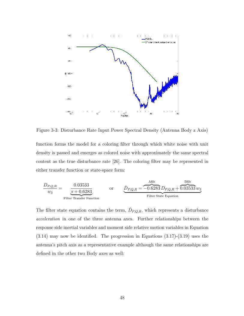
Figure 3-3: Disturbance Rate Input Power Spectral Density (Antenna Body z Axis)
function forms the model for a coloring filter through which white noise with unit
density is passed and emerges as colored noise with approximately the same spectral
content as the true disturbance rate [26]. The coloring filter may be represented in
either transfer function or state-space form:
DP,Q,R
w3
=0.03533
s+ 0.6283︸ ︷︷ ︸Filter Transfer Function
or DP,Q,R =
Afilt︷ ︸︸ ︷−0.6283DP,Q,R +
Bfilt︷ ︸︸ ︷0.03533w3︸ ︷︷ ︸
Filter State Equation
The filter state equation contains the term, DP,Q,R, which represents a disturbance
acceleration in one of the three antenna axes. Further relationships between the
response side inertial variables and moment side relative motion variables in Equation
(3.14) may now be identified. The progression in Equations (3.17)-(3.19) uses the
antenna’s pitch axis as a representative example although the same relationships are
defined in the other two Body axes as well:
48
IyyQ = Iyy(θpitch + DQ) =∑y
Tmotor +∑y
Tdisturbance (3.17)
Q = θpitch +DQ (3.18)
q = θpitch +
∫DQ (3.19)
where q is the inertial pointing error angle away from the stationary operating point
(terminal to satellite pointing vector) about the y Body axis and∫DQ is the relative
angular position of the aircraft from the pointing vector about the y Body axis.
Similarly, p and r define inertial error angles away from the pointing vector in the x
and z Body axes respectively while∫DP and
∫DR represent relative aircraft angular
positions away from the pointing vector in the x and z Body axes respectively. At
this point a definition for total inertial pointing error may be defined as in (3.20)
where ∆ is the total inertial pointing error. Note that p does not affect the inertial
pointing error as the antenna’s roll motion cannot induce mispointing.
∆ =√q2 + r2 (3.20)
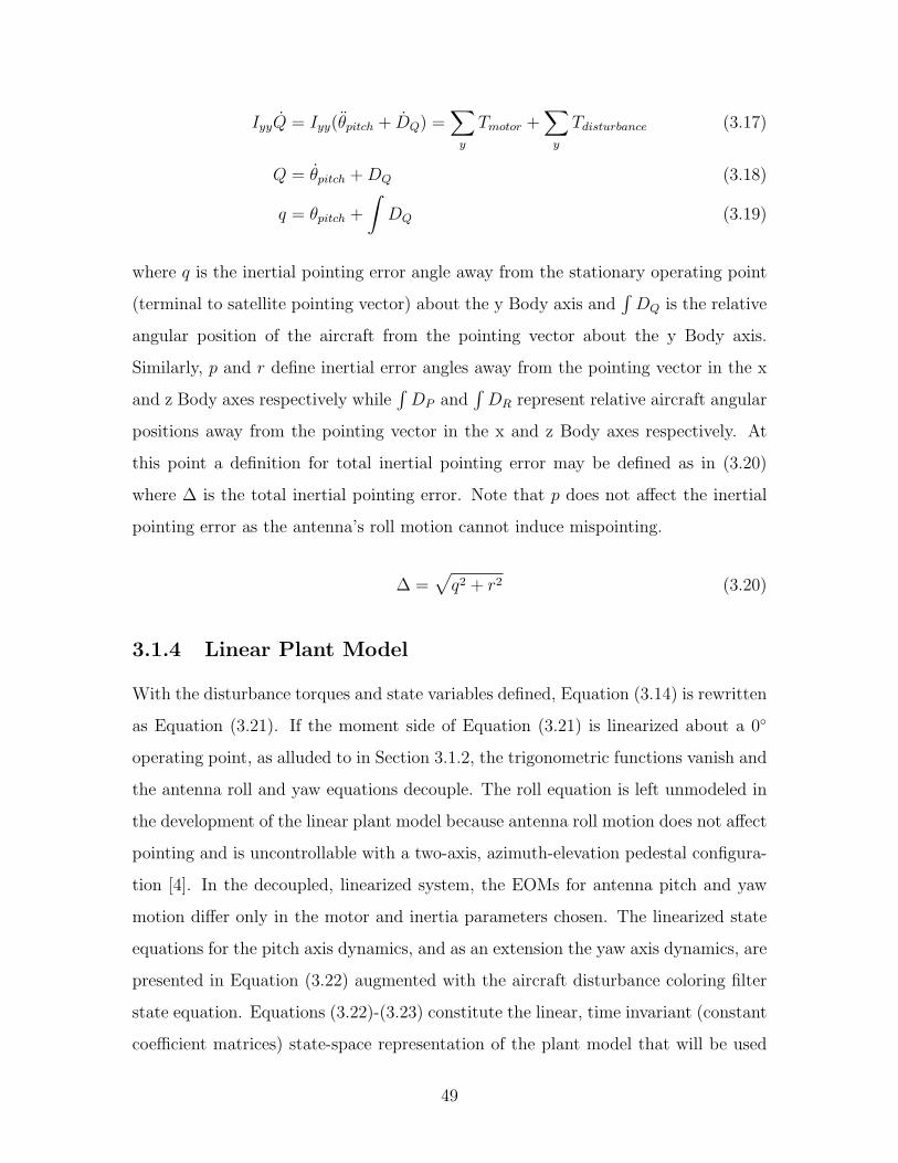
3.1.4 Linear Plant Model
With the disturbance torques and state variables defined, Equation (3.14) is rewritten
as Equation (3.21). If the moment side of Equation (3.21) is linearized about a 0
operating point, as alluded to in Section 3.1.2, the trigonometric functions vanish and
the antenna roll and yaw equations decouple. The roll equation is left unmodeled in
the development of the linear plant model because antenna roll motion does not affect
pointing and is uncontrollable with a two-axis, azimuth-elevation pedestal configura-
tion [4]. In the decoupled, linearized system, the EOMs for antenna pitch and yaw
motion differ only in the motor and inertia parameters chosen. The linearized state
equations for the pitch axis dynamics, and as an extension the yaw axis dynamics, are
presented in Equation (3.22) augmented with the aircraft disturbance coloring filter
state equation. Equations (3.22)-(3.23) constitute the linear, time invariant (constant
coefficient matrices) state-space representation of the plant model that will be used
49
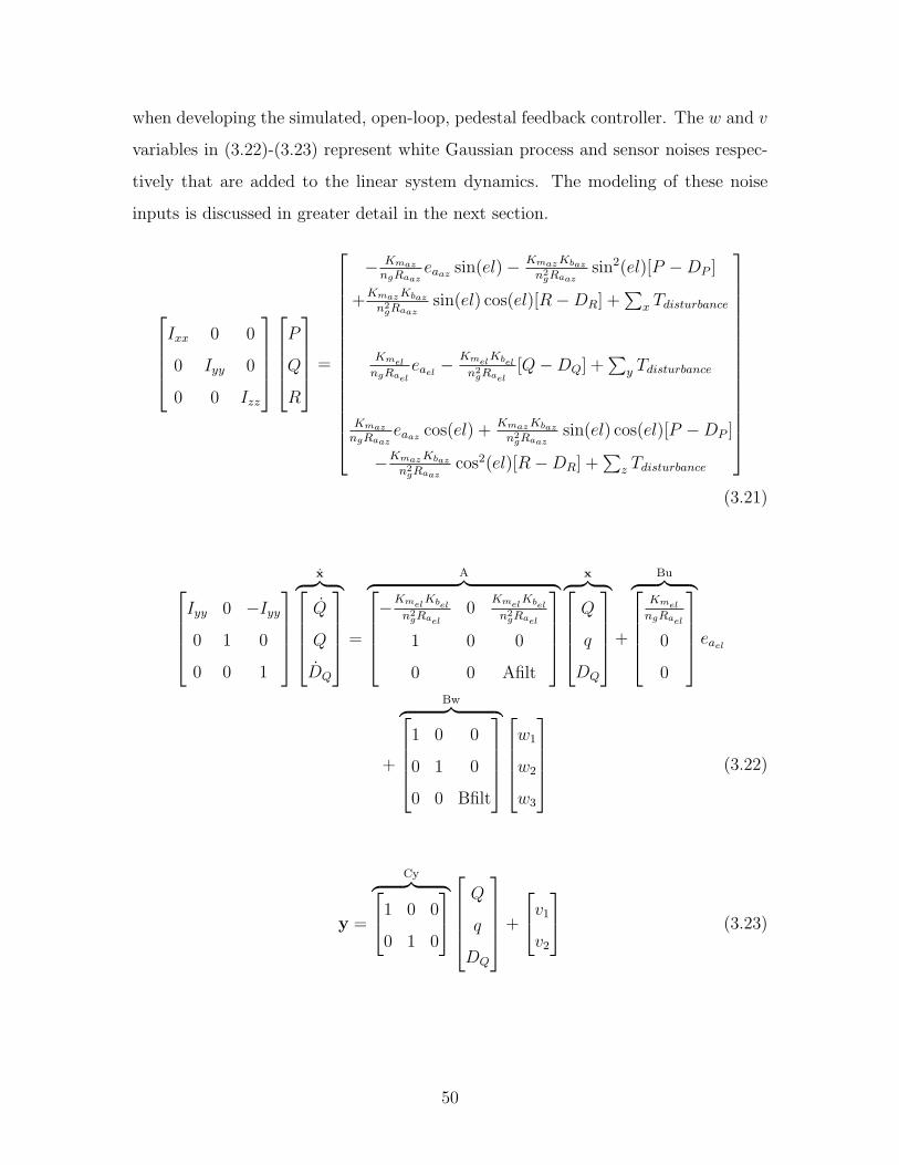
when developing the simulated, open-loop, pedestal feedback controller. The w and v
variables in (3.22)-(3.23) represent white Gaussian process and sensor noises respec-
tively that are added to the linear system dynamics. The modeling of these noise
inputs is discussed in greater detail in the next section.
Ixx 0 0
0 Iyy 0
0 0 Izz
P
Q
R
=
− KmazngRaaz
eaaz sin(el)− KmazKbazn2gRaaz
sin2(el)[P −DP ]
+KmazKbazn2gRaaz
sin(el) cos(el)[R−DR] +∑
x Tdisturbance
KmelngRael
eael −KmelKbeln2gRael
[Q−DQ] +∑
y Tdisturbance
KmazngRaaz
eaaz cos(el) +KmazKbazn2gRaaz
sin(el) cos(el)[P −DP ]
−KmazKbazn2gRaaz
cos2(el)[R−DR] +∑
z Tdisturbance
(3.21)
Iyy 0 −Iyy0 1 0
0 0 1
x︷ ︸︸ ︷Q
Q
DQ
=
A︷ ︸︸ ︷−KmelKbel
n2gRael
0KmelKbeln2gRael
1 0 0
0 0 Afilt
x︷ ︸︸ ︷Q
q
DQ
+
Bu︷ ︸︸ ︷KmelngRael
0
0
eael
+
Bw︷ ︸︸ ︷1 0 0
0 1 0
0 0 Bfilt
w1
w2
w3
(3.22)
y =
Cy︷ ︸︸ ︷1 0 0
0 1 0
Q
q
DQ
+
v1
v2
(3.23)
50
3.2 Controller Development and Simulation
Several approaches to developing feedback controllers for the pedestal motors are
available to the engineer. Classical control methods using Proportional Integral
Derivative (PID) tools and frequency-domain techniques, such as lead and lag filter
designs, are prevalent in industry and are often applied for use with DC servo-motors.
However, classical control design techniques do not take limitations on control efforts,
such as motor torques or armature voltages, into account and typically require many
iterations to reach an acceptable end design. The limitations of classical control the-
ory have, in part, led to the proliferation of state-space controller design techniques.
State-space techniques also serve as the tool for developing controllers for multiple-
input multiple-output (MIMO) systems. Because the aircraft motion disturbance
state, process noises, and sensor noises are present, the linear plant model developed
in Section 3.1.4 becomes a MIMO system. A deterministic, linear, time-invariant
state-space system representation takes the form:
x(t) = Ax(t) +Buu(t) (3.24)
y(t) = Cyx(t) +Du(t) (3.25)
Equations (3.22) and (3.23) resemble Equations (3.24) and (3.25) if the process and
sensor noises in the linearized plant model are neglected. Here, x is the state vector,
u is the control input vector, and y is the system output vector.
The main precept behind state-space control techniques involves the use of state
variable feedback in which combinations of the variables in the state vector, x, are fed
back into the system as control inputs through a gain matrix, K, in order to achieve
the desired closed loop system response. Using state variable feedback, the negative
feedback control law becomes:
u(t) = −K(t)x(t) (3.26)
51
Assuming that the state vector is deterministic and perfectly measurable, this strategy
allows the engineer to place the poles of the closed-loop system anywhere on the s-
plane by adjusting the values of the gains inside the K matrix accordingly, a technique
known as pole-placement [26,27]. Changing the location of the closed-loop poles in the
s-plane directly impacts the speed and nature of the closed-loop system’s response [23].
For the pedestal control system, it is desirable for the closed loop system poles to be
in the Left Half-Plane (LHP) of the s-plane to ensure system stability. The poles
must also lay far enough to the left of the origin of the s-plane so that perturbations
in the system states, specifically the yaw and pitch components of pointing error, are
quickly driven to zero. Moving the closed-loop system’s poles farther into the LHP
requires greater control effort, so a balance between speed of response and amount
of control input must be determined. The pole placement technique provides the
engineer with a useful tool, but pole placement alone offers no strategy as to where
exactly in the LHP the poles of the closed loop system should be placed. The optimal
control technique known as Linear-Quadratic Gaussian design (also called H2 design)
solves this problem by weighing the cost of control efforts against desired system
response, in the presence of system and measurement uncertainties, in the design of
the controller. An LQG controller will be designed for the nominal APS from Section
2.3 after the theory behind LQG controller design is briefly discussed.
3.2.1 Linear-Quadratic Regulation Theory
For linearized plant models, a quadratic cost functional may be developed that pe-
nalizes both state vector perturbations and applied control efforts. In the context
of the pedestal controller system, the state perturbations of greatest concern are the
pointing errors in the antenna yaw and pitch directions. The control efforts are the
applied voltages to the azimuth and elevation servo-motor circuits which cause applied
torques on the pedestal’s gimbals. A quadratic cost functional is justified because it
has the general effect of keeping a linear system model as honest as possible [27]. The
52
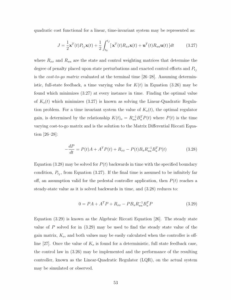
quadratic cost functional for a linear, time-invariant system may be represented as:
J =1
2xT (t)Ptfx(t) +
1
2
∫ tf
t0
[ xT (t)Rxxx(t) + uT (t)Ruuu(t) ]dt (3.27)
where Rxx and Ruu are the state and control weighting matrices that determine the
degree of penalty placed upon state perturbations and exacted control efforts and Ptf
is the cost-to-go matrix evaluated at the terminal time [26–28]. Assuming determin-
istic, full-state feedback, a time varying value for K(t) in Equation (3.26) may be
found which minimizes (3.27) at every instance in time. Finding the optimal value
of Ko(t) which minimizes (3.27) is known as solving the Linear-Quadratic Regula-
tion problem. For a time invariant system the value of Ko(t), the optimal regulator
gain, is determined by the relationship K(t)o = R−1uuB
Tu P (t) where P (t) is the time
varying cost-to-go matrix and is the solution to the Matrix Differential Riccati Equa-
tion [26–28]:
−dPdt
= P (t)A+ ATP (t) +Rxx − P (t)BuR−1uuB
Tu P (t) (3.28)
Equation (3.28) may be solved for P (t) backwards in time with the specified boundary
condition, Ptf , from Equation (3.27). If the final time is assumed to be infinitely far
off, an assumption valid for the pedestal controller application, then P (t) reaches a
steady-state value as it is solved backwards in time, and (3.28) reduces to:
0 = PA+ ATP +Rxx − PBuR−1uuB
Tu P (3.29)
Equation (3.29) is known as the Algebraic Riccati Equation [26]. The steady state
value of P solved for in (3.29) may be used to find the steady state value of the
gain matrix, Ko, and both values may be easily calculated when the controller is off-
line [27]. Once the value of Ko is found for a deterministic, full state feedback case,
the control law in (3.26) may be implemented and the performance of the resulting
controller, known as the Linear-Quadratic Regulator (LQR), on the actual system
may be simulated or observed.
53
3.2.2 Linear-Quadratic Estimation Theory
In most LQR systems, the assumptions that the state vector can be fully measured
and that the system is deterministic do not hold, and the regulator must be augmented
with a state estimator. For example, the linearized pedestal plant model for either the
antenna pitch or yaw axis dynamics presented in Equations (3.22)–(3.23) contains an
immeasurable disturbance rate input state, DQ,P , which must be estimated. Modeling
errors, actuator disturbances, and the effects of non-linearities on a linearized system
plant constitute process noises, and any errors in the sensing of the measured states
may be added to the plant model as sensor noises [27]. Process and sensor noises
make the modeled dynamics of the given linear, time-invariant plant a stochastic one
which may be represented as
x(t) = Ax(t) +Buu(t) +Bww(t) (3.30)
y(t) = Cyx(t) +Du(t) + v(t) (3.31)
where w(t) represents process noise inputs to the system and v(t) represents sensor
noise. The system representation in Equations (3.30)–(3.31) describes the system
in Equations (3.22)–(3.23) if (3.22) were multiplied through by the inverse of the
inertia matrix. If information is known about the structures of the noises, then the
noise dynamics may be modeled and augmented with the linear system model as
shown in Section 3.1.3. If no information about the noises’ structures is known, they
may be assumed to be white Gaussian noise processes. The assumption of white
Gaussian noise is a worst-case scenario [27]. The white noise inputs to the stochastic
system plant have covariance intensity matrices Rww and Rvv for process and sensor
noises respectively. Using white noise with specified intensities provides a means
of culminating the uncertainties in the linear system into “catch-all” factors. It is
desirable to develop an estimator to approximate the state variables with the minimal
amount of estimation error while optimally balancing the effects of both process and
sensor noises in the system. The estimated state vector is written as x and the est-
54
imation error as x (Equations (3.32) and (3.33)). The estimation dynamics for a
linear, time-invariant system may be written as
˙x(t) = Ax(t) +Buu(t) + L(t)(y(t)− Cyx(t)) (3.32)
x = x− x (3.33)
where L(t) is the estimator gain applied to the innovation or difference between
measured and predicted system outputs. The estimator gain determines where in the
LHP the estimator poles are located. Generally, it is desirable for the estimator poles
to be faster than the regulator poles so that the estimated state vector may be used for
regulator feedback without introducing large errors. The Kalman-Bucy filter provides
the optimal solution to the Linear-Quadratic Estimation problem and decides where
in the LHP the estimator poles should be placed based on the relative intensities of the
process and sensor noises. Applying the Kalman-Bucy filter, the value of Lo(t), the
optimal estimator gain, is governed by the relationship Lo(t) = Q(t)CTy R−1vv [26, 27].
The estimation error covariance matrix, Q(t), is found from the solution of the Matrix
Differential Riccati equation:
dQ
dt= AQ(t) +Q(t)AT +BwRwwB
Tw −Q(t)CT
y R−1vv CyQ(t) (3.34)
Equations (3.28) and (3.34) bear strong resemblance to each other and are, in fact,
mathematical duals [26,27]. The steady-state value of Q may be found by the solution
of the Algebraic Riccati Equation, (3.35), if the initial time is assumed to have oc-
curred in the distant past [27], an assumption that is generally valid for the pedestal
control application.
0 = AQ+QAT +BwRwwBTw −QCT
y R−1vv CyQ (3.35)
55
3.2.3 Linear-Quadratic Gaussian Theory
The separation principle states that the optimal regulator and estimator gains can
be solved for independently [29]. The resulting Linear-Quadratic Gaussian (LQG)
controller dynamics may be written as
˙x(t) = (A−BuKo − LoCy)x(t) + Lo(t)y(t) (3.36)
u = −Kox (3.37)
where the estimated plant state, x(t), is also the controller state variable [26, 27].
The controller dynamics may be augmented with the linear system plant dynamics
to form the closed-loop system. The poles of the closed-loop, linear system, which
govern the nature and speed of the system’s response, are simply the union of the
regulator and estimator poles. The closed loop poles of the regulator may be found
by calculating the eigenvalues of the (A − BuKo) matrix, and the estimator poles
are found by solving for the eigenvalues of the (A − LoCy) matrix. Equation (3.37)
highlights the new control law for the LQG controller, u(t) = −Kox(t), which is
actually the optimal feedback strategy for the stochastic Linear-Quadratic control
problem. For a proof of the optimality of the LQG control strategy, the reader is
referred to the literature [26,30].
3.2.4 Reference Commands
The ability for the pedestal controller to track an input reference command is needed
in order to slew the antenna to various positions in the sky to track different target
satellites and to intelligently dither the antenna’s mainlobe in order to implement a
closed-loop pointing strategy. Perhaps the best strategy for implementing a reference
command in an LQG controller is to ensure that the estimation error is independent
of the reference command [31]. This strategy is accomplished by changing the form
of the controller dynamics in Equations (3.36)–(3.37) so that the controller explicitly
has two inputs, the measurement states, y, and the reference command, r (3.38). The
56
feedback control law is also changed to incorporate the reference command (3.39).
˙x(t) = (A−BuKo − LoCy)x(t) + Lo(t)y(t) +BuNr (3.38)
u = −Kox + Nr (3.39)
Finally, the N matrix is selected such that the gain of the closed-loop transfer function
Y(s)/R(s) equals one at DC which ensures accurate steady-state tracking of an input
reference command [31].
3.2.5 Development of the LQG Pedestal Controller in
MATLAB
This section develops an LQG pedestal feedback controller for the nominal APS with
the aid of the MATLAB programming language. MATLAB is a scripting language
used for technical computing and for developing visualizations and simulations. The
MATLAB script referenced in this section uses several predefined functions found in
MATLAB’s Control System Toolbox. The MATLAB m-file ‘controller.m’, found in
Appendix B.1, implements an LQG controller for the elevation motor of the nomi-
nal APS pedestal. The linearized plant model used in the controller’s development
is described by Equations (3.22)–(3.23), and the motor parameters used are those
published in the specifications sheet for the Cleveland Motion Controls 2115 servo-
motor with an F winding [20]. As an approximation to the moments of inertia for
the combined antenna and elevation gimbal assembly, the calculated inertias of the
24 in. dish antenna are used in the derivation of the LQG controller. Because the
same linearized plant model presented in Equations (3.22)–(3.23) is used to describe
both the antenna’s yaw and pitch dynamics, ‘controller.m’ is also used to develop
the controller for the azimuth servo-motor. The nominal APS uses the same mo-
tors in both the azimuth and elevation axes, so the motor parameters do not change
for the development of the azimuth motor controller. Also, because the Iyy and Izz
moments of inertia for the 24 in. dish are equal, and the inertia of the dish is used
57
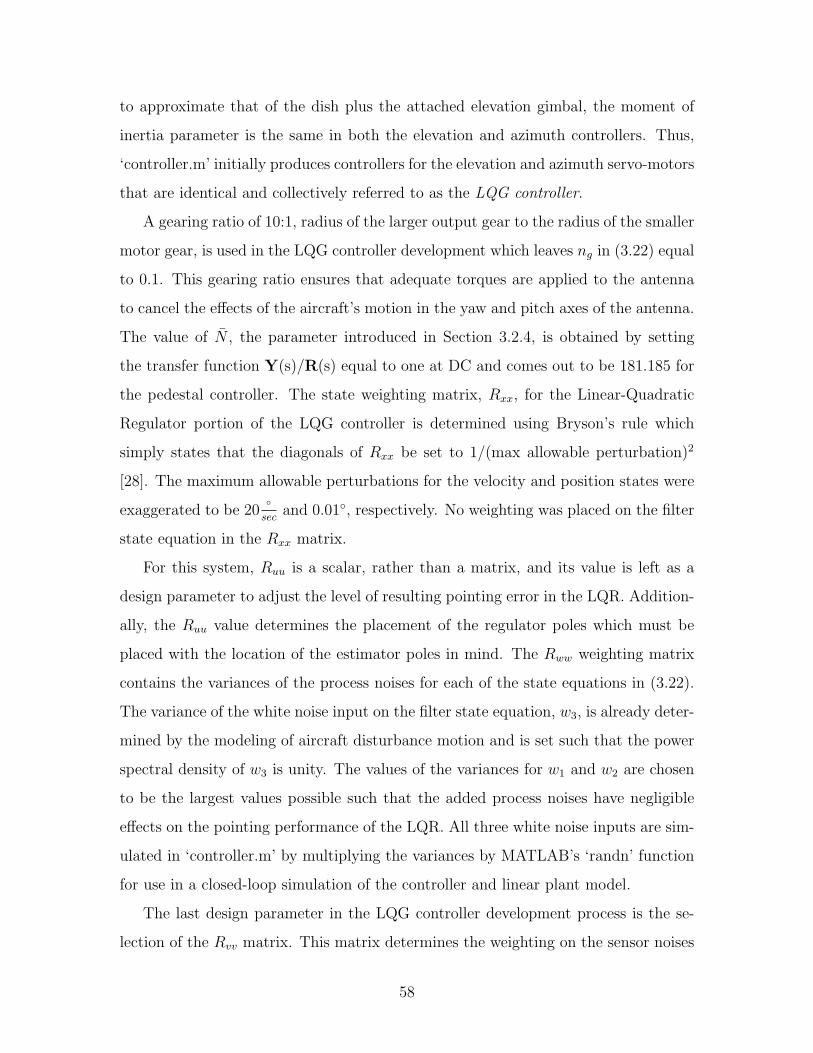
to approximate that of the dish plus the attached elevation gimbal, the moment of
inertia parameter is the same in both the elevation and azimuth controllers. Thus,
‘controller.m’ initially produces controllers for the elevation and azimuth servo-motors
that are identical and collectively referred to as the LQG controller.
A gearing ratio of 10:1, radius of the larger output gear to the radius of the smaller
motor gear, is used in the LQG controller development which leaves ng in (3.22) equal
to 0.1. This gearing ratio ensures that adequate torques are applied to the antenna
to cancel the effects of the aircraft’s motion in the yaw and pitch axes of the antenna.
The value of N , the parameter introduced in Section 3.2.4, is obtained by setting
the transfer function Y(s)/R(s) equal to one at DC and comes out to be 181.185 for
the pedestal controller. The state weighting matrix, Rxx, for the Linear-Quadratic
Regulator portion of the LQG controller is determined using Bryson’s rule which
simply states that the diagonals of Rxx be set to 1/(max allowable perturbation)2
[28]. The maximum allowable perturbations for the velocity and position states were
exaggerated to be 20
secand 0.01, respectively. No weighting was placed on the filter
state equation in the Rxx matrix.
For this system, Ruu is a scalar, rather than a matrix, and its value is left as a
design parameter to adjust the level of resulting pointing error in the LQR. Addition-
ally, the Ruu value determines the placement of the regulator poles which must be
placed with the location of the estimator poles in mind. The Rww weighting matrix
contains the variances of the process noises for each of the state equations in (3.22).
The variance of the white noise input on the filter state equation, w3, is already deter-
mined by the modeling of aircraft disturbance motion and is set such that the power
spectral density of w3 is unity. The values of the variances for w1 and w2 are chosen
to be the largest values possible such that the added process noises have negligible
effects on the pointing performance of the LQR. All three white noise inputs are sim-
ulated in ‘controller.m’ by multiplying the variances by MATLAB’s ‘randn’ function
for use in a closed-loop simulation of the controller and linear plant model.
The last design parameter in the LQG controller development process is the se-
lection of the Rvv matrix. This matrix determines the weighting on the sensor noises
58
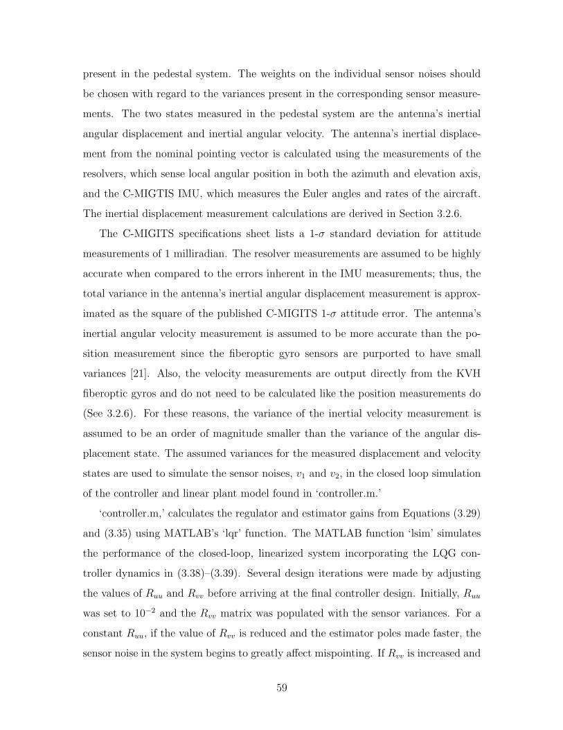
present in the pedestal system. The weights on the individual sensor noises should
be chosen with regard to the variances present in the corresponding sensor measure-
ments. The two states measured in the pedestal system are the antenna’s inertial
angular displacement and inertial angular velocity. The antenna’s inertial displace-
ment from the nominal pointing vector is calculated using the measurements of the
resolvers, which sense local angular position in both the azimuth and elevation axis,
and the C-MIGTIS IMU, which measures the Euler angles and rates of the aircraft.
The inertial displacement measurement calculations are derived in Section 3.2.6.
The C-MIGITS specifications sheet lists a 1-σ standard deviation for attitude
measurements of 1 milliradian. The resolver measurements are assumed to be highly
accurate when compared to the errors inherent in the IMU measurements; thus, the
total variance in the antenna’s inertial angular displacement measurement is approx-
imated as the square of the published C-MIGITS 1-σ attitude error. The antenna’s
inertial angular velocity measurement is assumed to be more accurate than the po-
sition measurement since the fiberoptic gyro sensors are purported to have small
variances [21]. Also, the velocity measurements are output directly from the KVH
fiberoptic gyros and do not need to be calculated like the position measurements do
(See 3.2.6). For these reasons, the variance of the inertial velocity measurement is
assumed to be an order of magnitude smaller than the variance of the angular dis-
placement state. The assumed variances for the measured displacement and velocity
states are used to simulate the sensor noises, v1 and v2, in the closed loop simulation
of the controller and linear plant model found in ‘controller.m.’
‘controller.m,’ calculates the regulator and estimator gains from Equations (3.29)
and (3.35) using MATLAB’s ‘lqr’ function. The MATLAB function ‘lsim’ simulates
the performance of the closed-loop, linearized system incorporating the LQG con-
troller dynamics in (3.38)–(3.39). Several design iterations were made by adjusting
the values of Ruu and Rvv before arriving at the final controller design. Initially, Ruu
was set to 10−2 and the Rvv matrix was populated with the sensor variances. For a
constant Ruu, if the value of Rvv is reduced and the estimator poles made faster, the
sensor noise in the system begins to greatly affect mispointing. If Rvv is increased and
59
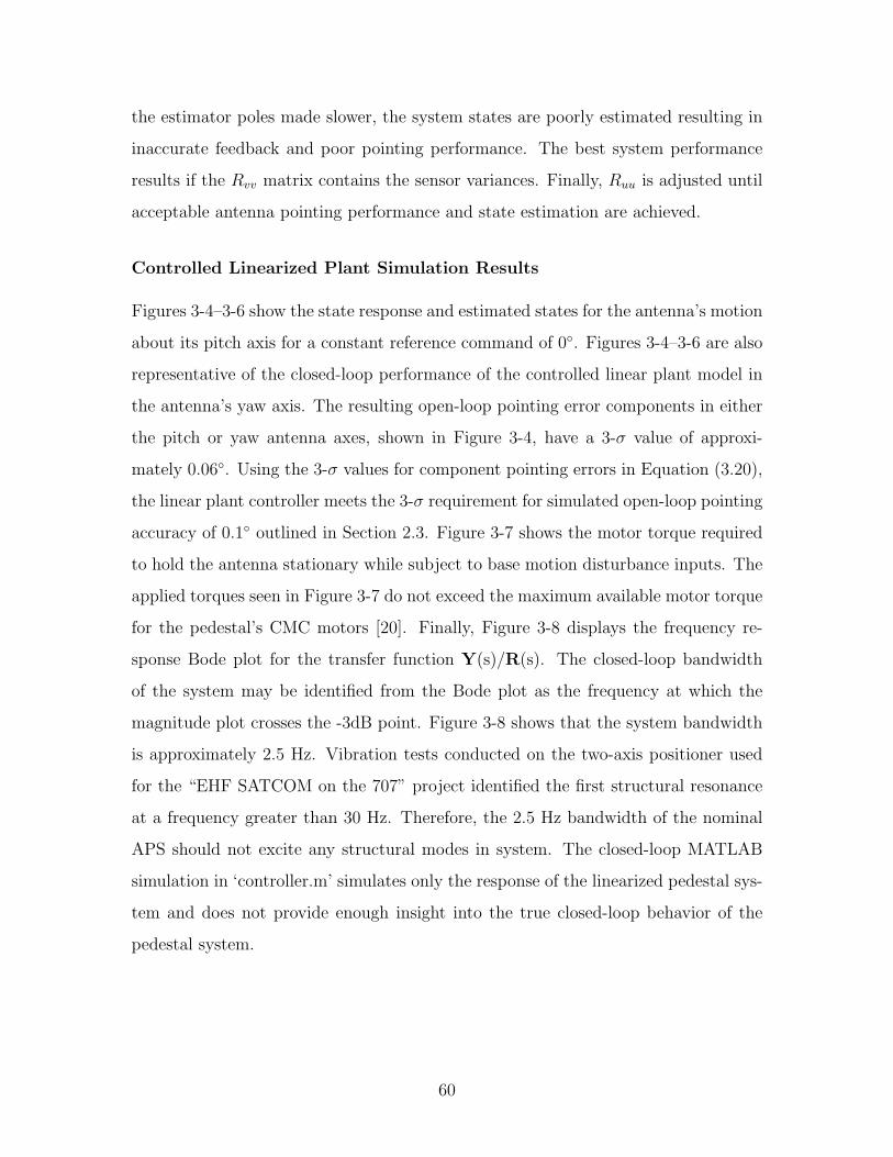
the estimator poles made slower, the system states are poorly estimated resulting in
inaccurate feedback and poor pointing performance. The best system performance
results if the Rvv matrix contains the sensor variances. Finally, Ruu is adjusted until
acceptable antenna pointing performance and state estimation are achieved.
Controlled Linearized Plant Simulation Results
Figures 3-4–3-6 show the state response and estimated states for the antenna’s motion
about its pitch axis for a constant reference command of 0. Figures 3-4–3-6 are also
representative of the closed-loop performance of the controlled linear plant model in
the antenna’s yaw axis. The resulting open-loop pointing error components in either
the pitch or yaw antenna axes, shown in Figure 3-4, have a 3-σ value of approxi-
mately 0.06. Using the 3-σ values for component pointing errors in Equation (3.20),
the linear plant controller meets the 3-σ requirement for simulated open-loop pointing
accuracy of 0.1 outlined in Section 2.3. Figure 3-7 shows the motor torque required
to hold the antenna stationary while subject to base motion disturbance inputs. The
applied torques seen in Figure 3-7 do not exceed the maximum available motor torque
for the pedestal’s CMC motors [20]. Finally, Figure 3-8 displays the frequency re-
sponse Bode plot for the transfer function Y(s)/R(s). The closed-loop bandwidth
of the system may be identified from the Bode plot as the frequency at which the
magnitude plot crosses the -3dB point. Figure 3-8 shows that the system bandwidth
is approximately 2.5 Hz. Vibration tests conducted on the two-axis positioner used
for the “EHF SATCOM on the 707” project identified the first structural resonance
at a frequency greater than 30 Hz. Therefore, the 2.5 Hz bandwidth of the nominal
APS should not excite any structural modes in system. The closed-loop MATLAB
simulation in ‘controller.m’ simulates only the response of the linearized pedestal sys-
tem and does not provide enough insight into the true closed-loop behavior of the
pedestal system.
60
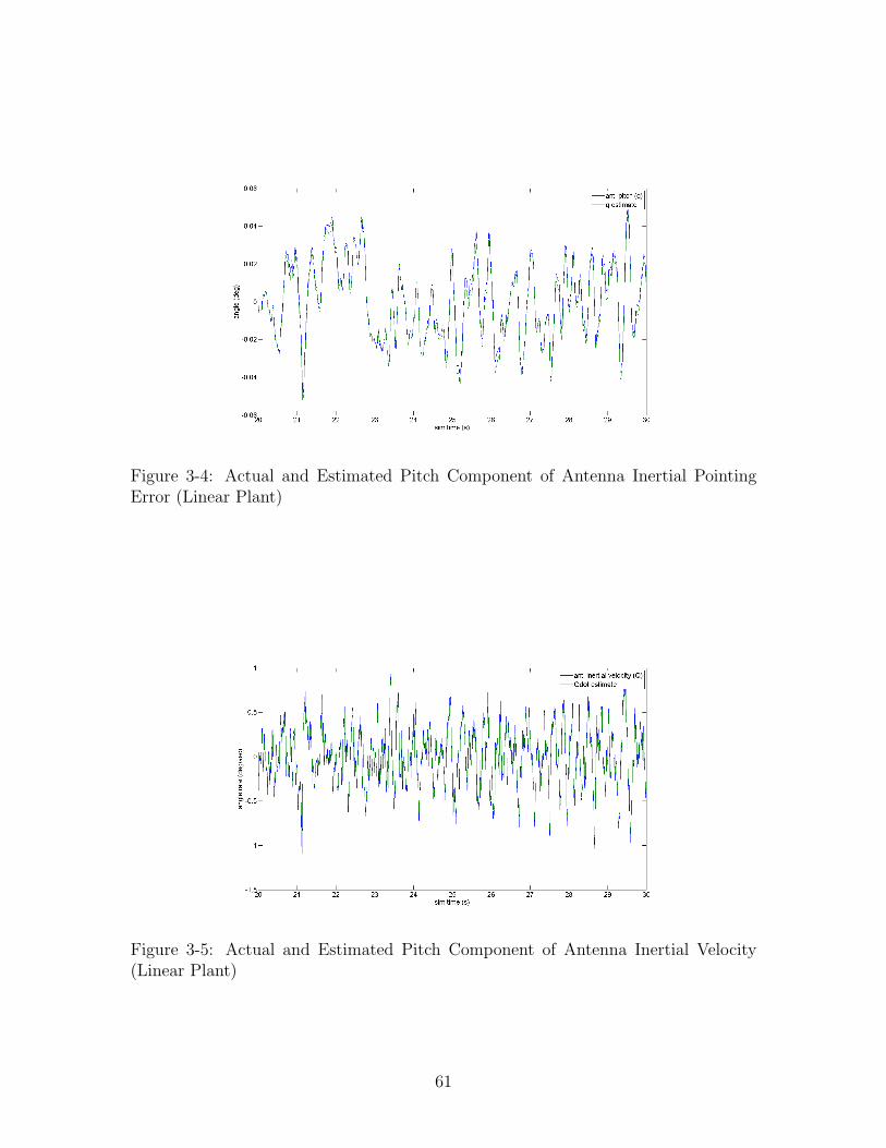
Figure 3-4: Actual and Estimated Pitch Component of Antenna Inertial PointingError (Linear Plant)
Figure 3-5: Actual and Estimated Pitch Component of Antenna Inertial Velocity(Linear Plant)
61
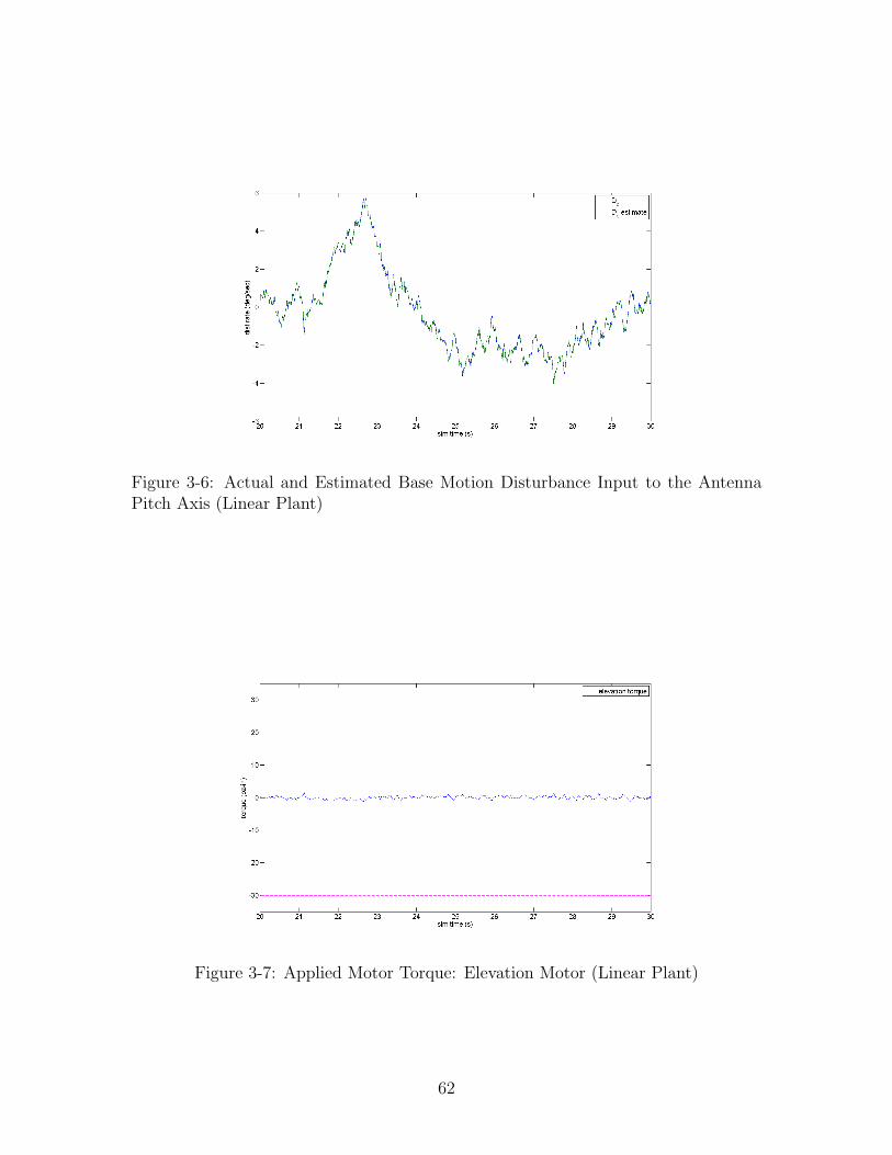
Figure 3-6: Actual and Estimated Base Motion Disturbance Input to the AntennaPitch Axis (Linear Plant)
Figure 3-7: Applied Motor Torque: Elevation Motor (Linear Plant)
62
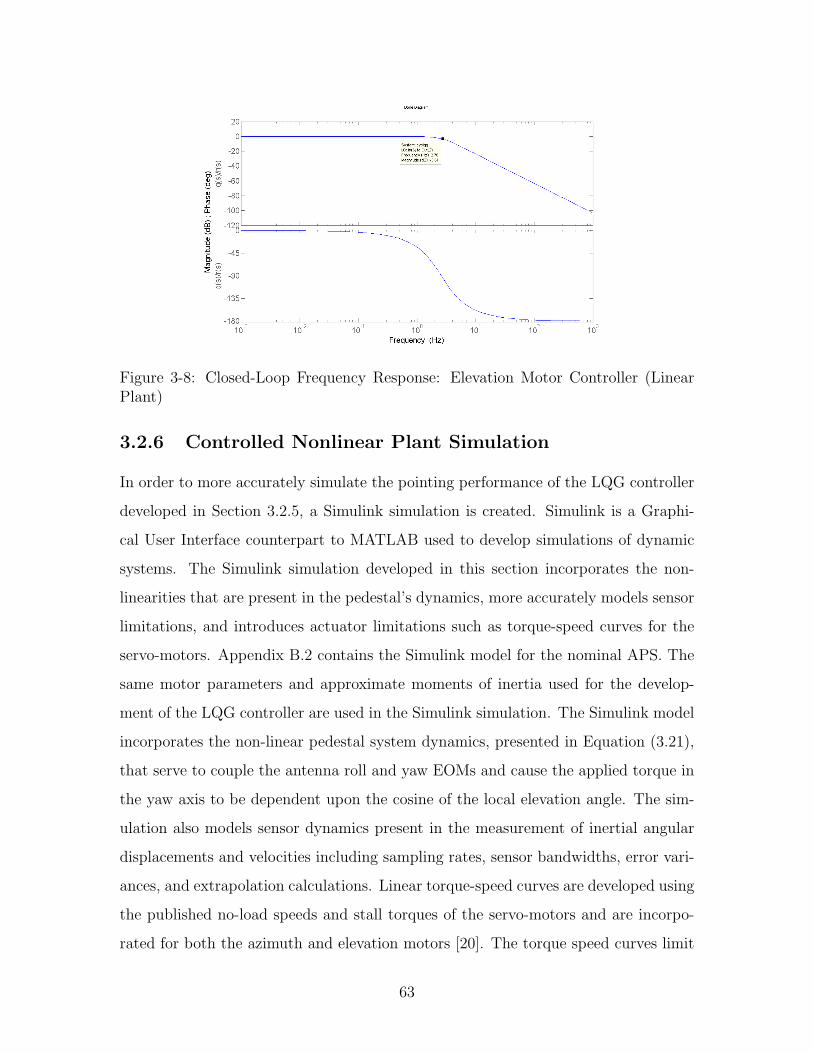
Figure 3-8: Closed-Loop Frequency Response: Elevation Motor Controller (LinearPlant)
3.2.6 Controlled Nonlinear Plant Simulation
In order to more accurately simulate the pointing performance of the LQG controller
developed in Section 3.2.5, a Simulink simulation is created. Simulink is a Graphi-
cal User Interface counterpart to MATLAB used to develop simulations of dynamic
systems. The Simulink simulation developed in this section incorporates the non-
linearities that are present in the pedestal’s dynamics, more accurately models sensor
limitations, and introduces actuator limitations such as torque-speed curves for the
servo-motors. Appendix B.2 contains the Simulink model for the nominal APS. The
same motor parameters and approximate moments of inertia used for the develop-
ment of the LQG controller are used in the Simulink simulation. The Simulink model
incorporates the non-linear pedestal system dynamics, presented in Equation (3.21),
that serve to couple the antenna roll and yaw EOMs and cause the applied torque in
the yaw axis to be dependent upon the cosine of the local elevation angle. The sim-
ulation also models sensor dynamics present in the measurement of inertial angular
displacements and velocities including sampling rates, sensor bandwidths, error vari-
ances, and extrapolation calculations. Linear torque-speed curves are developed using
the published no-load speeds and stall torques of the servo-motors and are incorpo-
rated for both the azimuth and elevation motors [20]. The torque speed curves limit
63
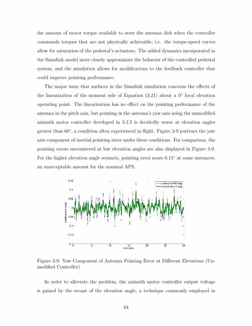
the amount of motor torque available to steer the antenna dish when the controller
commands torques that are not physically achievable, i.e. the torque-speed curves
allow for saturation of the pedestal’s actuators. The added dynamics incorporated in
the Simulink model more closely approximate the behavior of the controlled pedestal
system, and the simulation allows for modifications to the feedback controller that
could improve pointing performance.
The major issue that surfaces in the Simulink simulation concerns the effects of
the linearization of the moment side of Equation (3.21) about a 0 local elevation
operating point. The linearization has no effect on the pointing performance of the
antenna in the pitch axis, but pointing in the antenna’s yaw axis using the unmodified
azimuth motor controller developed in 3.2.5 is decidedly worse at elevation angles
greater than 60, a condition often experienced in flight. Figure 3-9 portrays the yaw
axis component of inertial pointing error under these conditions. For comparison, the
pointing errors encountered at low elevation angles are also displayed in Figure 3-9.
For the higher elevation angle scenario, pointing error nears 0.15 at some instances;
an unacceptable amount for the nominal APS.
Figure 3-9: Yaw Component of Antenna Pointing Error at Different Elevations (Un-modified Controller)
In order to alleviate the problem, the azimuth motor controller output voltage
is gained by the secant of the elevation angle, a technique commonly employed in
64
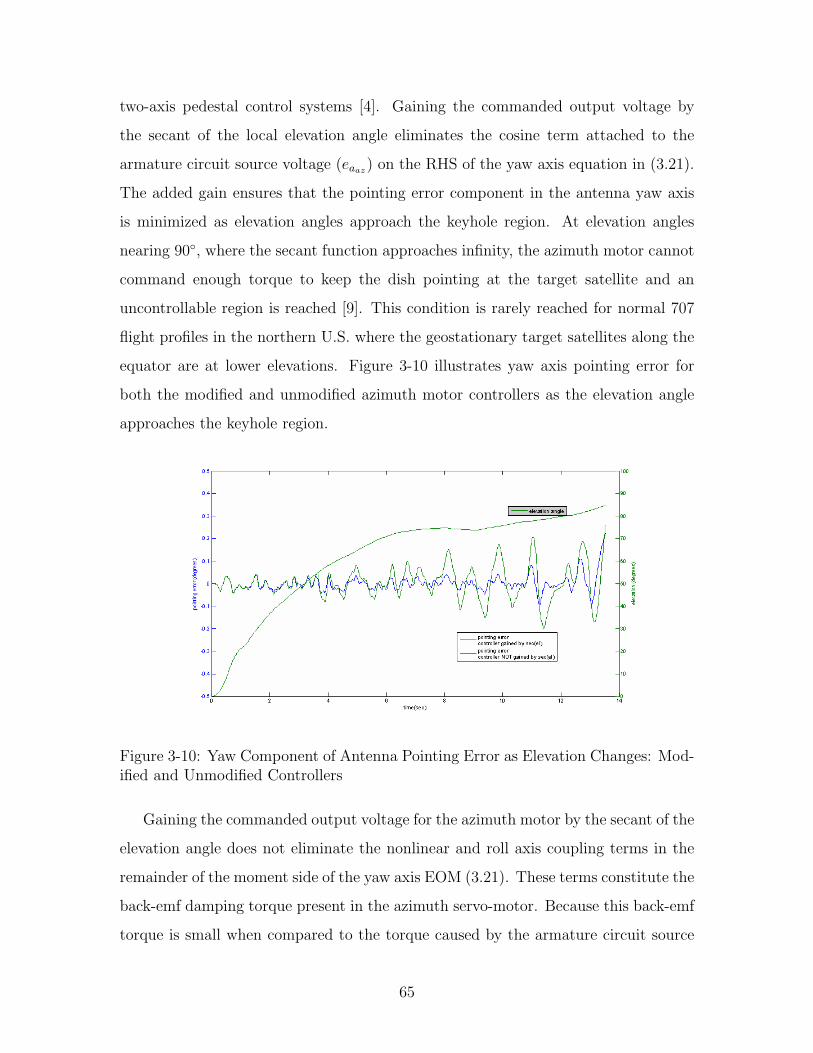
two-axis pedestal control systems [4]. Gaining the commanded output voltage by
the secant of the local elevation angle eliminates the cosine term attached to the
armature circuit source voltage (eaaz) on the RHS of the yaw axis equation in (3.21).
The added gain ensures that the pointing error component in the antenna yaw axis
is minimized as elevation angles approach the keyhole region. At elevation angles
nearing 90, where the secant function approaches infinity, the azimuth motor cannot
command enough torque to keep the dish pointing at the target satellite and an
uncontrollable region is reached [9]. This condition is rarely reached for normal 707
flight profiles in the northern U.S. where the geostationary target satellites along the
equator are at lower elevations. Figure 3-10 illustrates yaw axis pointing error for
both the modified and unmodified azimuth motor controllers as the elevation angle
approaches the keyhole region.
Figure 3-10: Yaw Component of Antenna Pointing Error as Elevation Changes: Mod-ified and Unmodified Controllers
Gaining the commanded output voltage for the azimuth motor by the secant of the
elevation angle does not eliminate the nonlinear and roll axis coupling terms in the
remainder of the moment side of the yaw axis EOM (3.21). These terms constitute the
back-emf damping torque present in the azimuth servo-motor. Because this back-emf
torque is small when compared to the torque caused by the armature circuit source
65
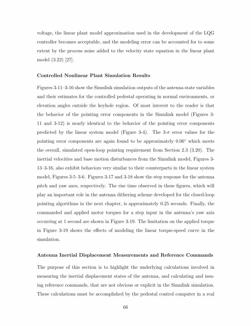
voltage, the linear plant model approximation used in the development of the LQG
controller becomes acceptable, and the modeling error can be accounted for to some
extent by the process noise added to the velocity state equation in the linear plant
model (3.22) [27].
Controlled Nonlinear Plant Simulation Results
Figures 3-11–3-16 show the Simulink simulation outputs of the antenna state variables
and their estimates for the controlled pedestal operating in normal environments, or
elevation angles outside the keyhole region. Of most interest to the reader is that
the behavior of the pointing error components in the Simulink model (Figures 3-
11 and 3-12) is nearly identical to the behavior of the pointing error components
predicted by the linear system model (Figure 3-4). The 3-σ error values for the
pointing error components are again found to be approximately 0.06 which meets
the overall, simulated open-loop pointing requirement from Section 2.3 (3.20). The
inertial velocities and base motion disturbances from the Simulink model, Figures 3-
13–3-16, also exhibit behaviors very similar to their counterparts in the linear system
model, Figures 3-5–3-6. Figures 3-17 and 3-18 show the step response for the antenna
pitch and yaw axes, respectively. The rise time observed in these figures, which will
play an important role in the antenna dithering scheme developed for the closed-loop
pointing algorithms in the next chapter, is approximately 0.25 seconds. Finally, the
commanded and applied motor torques for a step input in the antenna’s yaw axis
occurring at 1 second are shown in Figure 3-19. The limitation on the applied torque
in Figure 3-19 shows the effects of modeling the linear torque-speed curve in the
simulation.
Antenna Inertial Displacement Measurements and Reference Commands
The purpose of this section is to highlight the underlying calculations involved in
measuring the inertial displacement states of the antenna, and calculating and issu-
ing reference commands, that are not obvious or explicit in the Simulink simulation.
These calculations must be accomplished by the pedestal control computer in a real
66
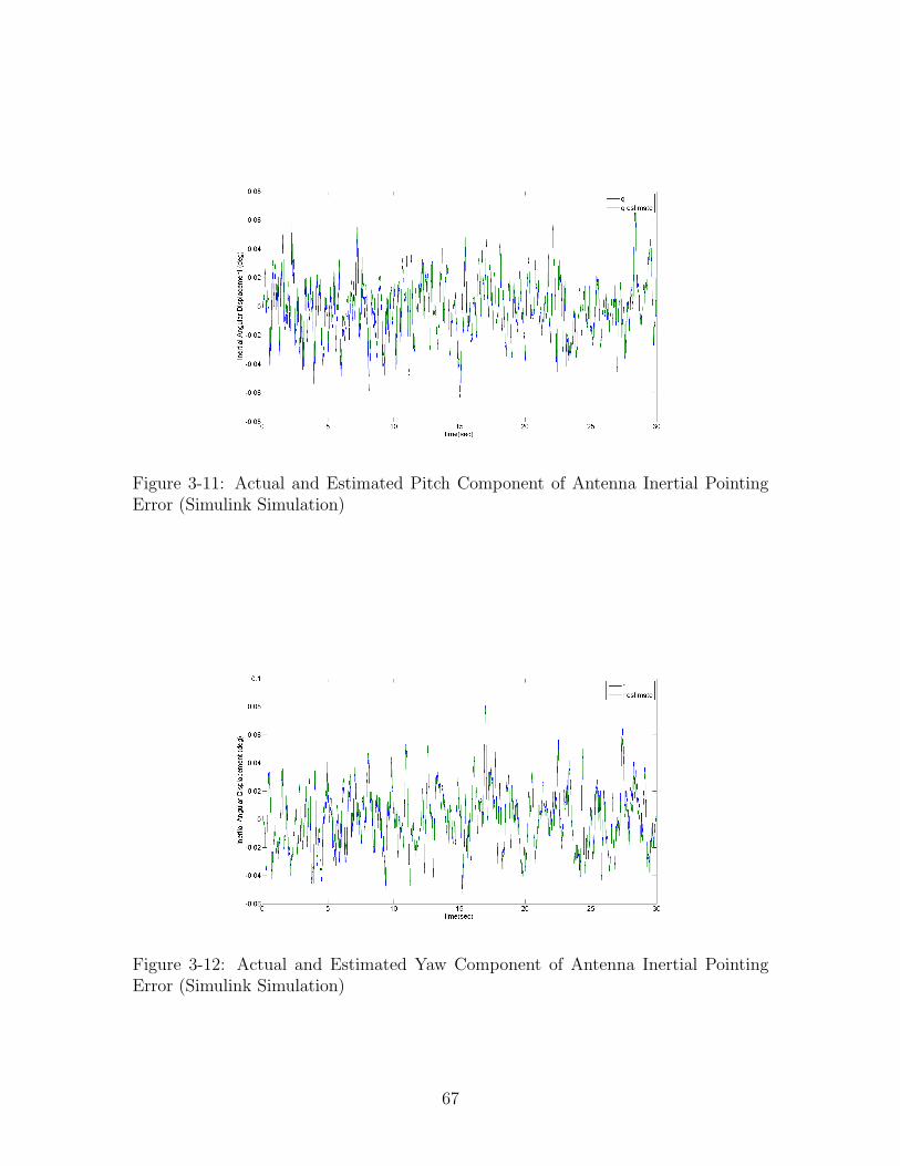
Figure 3-11: Actual and Estimated Pitch Component of Antenna Inertial PointingError (Simulink Simulation)
Figure 3-12: Actual and Estimated Yaw Component of Antenna Inertial PointingError (Simulink Simulation)
67
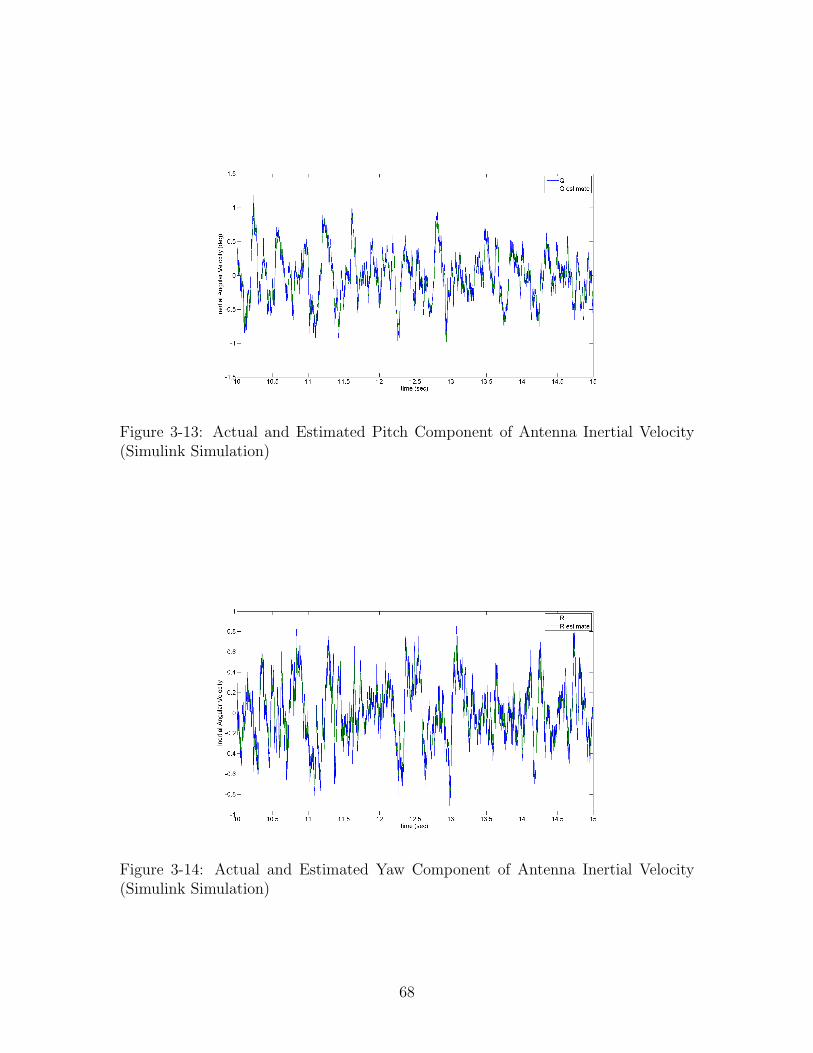
Figure 3-13: Actual and Estimated Pitch Component of Antenna Inertial Velocity(Simulink Simulation)
Figure 3-14: Actual and Estimated Yaw Component of Antenna Inertial Velocity(Simulink Simulation)
68
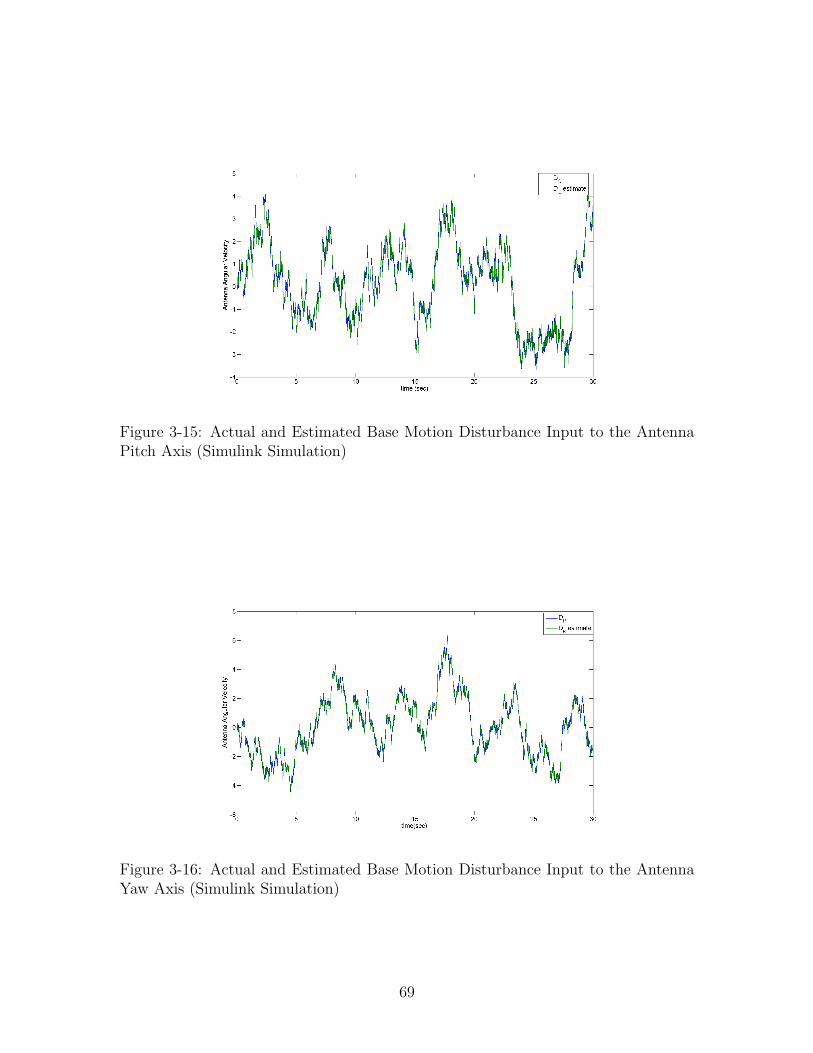
Figure 3-15: Actual and Estimated Base Motion Disturbance Input to the AntennaPitch Axis (Simulink Simulation)
Figure 3-16: Actual and Estimated Base Motion Disturbance Input to the AntennaYaw Axis (Simulink Simulation)
69
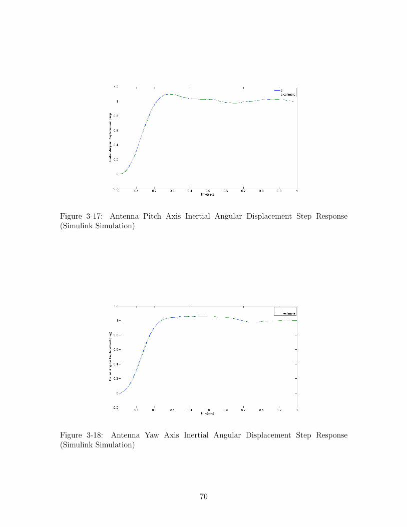
Figure 3-17: Antenna Pitch Axis Inertial Angular Displacement Step Response(Simulink Simulation)
Figure 3-18: Antenna Yaw Axis Inertial Angular Displacement Step Response(Simulink Simulation)
70
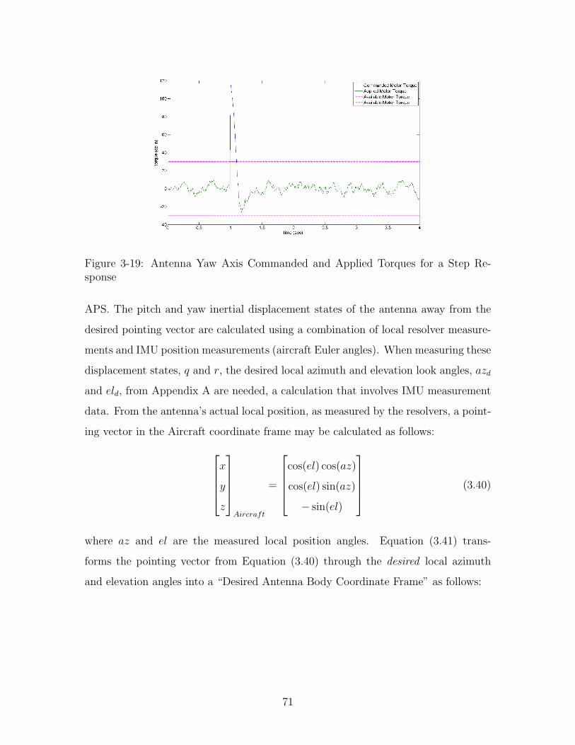
Figure 3-19: Antenna Yaw Axis Commanded and Applied Torques for a Step Re-sponse
APS. The pitch and yaw inertial displacement states of the antenna away from the
desired pointing vector are calculated using a combination of local resolver measure-
ments and IMU position measurements (aircraft Euler angles). When measuring these
displacement states, q and r, the desired local azimuth and elevation look angles, azd
and eld, from Appendix A are needed, a calculation that involves IMU measurement
data. From the antenna’s actual local position, as measured by the resolvers, a point-
ing vector in the Aircraft coordinate frame may be calculated as follows:x
y
z
Aircraft
=
cos(el) cos(az)
cos(el) sin(az)
− sin(el)
(3.40)
where az and el are the measured local position angles. Equation (3.41) trans-
forms the pointing vector from Equation (3.40) through the desired local azimuth
and elevation angles into a “Desired Antenna Body Coordinate Frame” as follows:
71
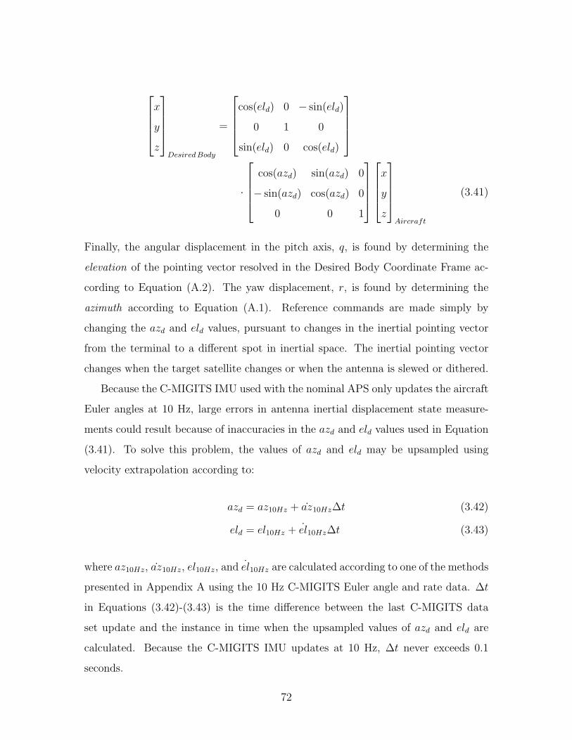
x
y
z
DesiredBody
=
cos(eld) 0 − sin(eld)
0 1 0
sin(eld) 0 cos(eld)
·
cos(azd) sin(azd) 0
− sin(azd) cos(azd) 0
0 0 1
x
y
z
Aircraft
(3.41)
Finally, the angular displacement in the pitch axis, q, is found by determining the
elevation of the pointing vector resolved in the Desired Body Coordinate Frame ac-
cording to Equation (A.2). The yaw displacement, r, is found by determining the
azimuth according to Equation (A.1). Reference commands are made simply by
changing the azd and eld values, pursuant to changes in the inertial pointing vector
from the terminal to a different spot in inertial space. The inertial pointing vector
changes when the target satellite changes or when the antenna is slewed or dithered.
Because the C-MIGITS IMU used with the nominal APS only updates the aircraft
Euler angles at 10 Hz, large errors in antenna inertial displacement state measure-
ments could result because of inaccuracies in the azd and eld values used in Equation
(3.41). To solve this problem, the values of azd and eld may be upsampled using
velocity extrapolation according to:
azd = az10Hz + az10Hz∆t (3.42)
eld = el10Hz + el10Hz∆t (3.43)
where az10Hz, az10Hz, el10Hz, and el10Hz are calculated according to one of the methods
presented in Appendix A using the 10 Hz C-MIGITS Euler angle and rate data. ∆t
in Equations (3.42)-(3.43) is the time difference between the last C-MIGITS data
set update and the instance in time when the upsampled values of azd and eld are
calculated. Because the C-MIGITS IMU updates at 10 Hz, ∆t never exceeds 0.1
seconds.
72
3.3 Pointing Error Distributions
In order to facilitate simulation of the performance of closed-loop pointing control
algorithms developed in the next chapter, an understanding of the statistical distri-
butions of the pitch and yaw components of pointing error must be developed. To
obtain data for modeling the distributions of q and r, the Simulink simulation from
Section 3.2.6 is run for 30 seconds and the pointing error components recorded at
evenly spaced time samples of 0.001 seconds (Figure 3-20). These points were then
used to construct auto-correlation functions to determine the time-scale at which the
pointing error distributions exhibit dependencies. The auto correlation functions are
plotted in Figures 3-21 and 3-22. Figures 3-21 and 3-22 show that the initial peaks of
the auto-correlation functions of the error components fall off at approximately 0.25
seconds. Thus, if the distributions of pointing error components prove to be normal,
every 0.25 seconds a pointing error component may be obtained that is nearly inde-
pendent of past pointing errors, assuming they occurred at 0.25 second intervals as
well [32].
After the correlation time is determined, the simulation is run again for 250 sec-
onds to record 1000 approximately independent samples of both the q and r pointing
error components. In an effort to compare the resulting samples to normal distribu-
tion curves, histograms are made of the data sets and plotted together with normal
distribution curves calculated from the sample means and variances. Figures 3-23 and
3-24 visually indicate the normalcy of the data; however, a statistical goodness-of-fit
test is required in order to be convinced that a normal approximation to the distri-
butions of the pointing error components accurately represents the true distributions
most of the time.
The Kolmogorov-Smirnoff goodness-of-fit test for normal distributions is applied
to the data sets of length 1000 where the population mean and variance are estimated
by the sample mean and variance [33]. The Kolmogorov-Smirnoff test weighs the null
hypothesis (H0), that claims the sample data has a normal distribution, against the
alternate hypothesis (Ha) that states the data is not from a normal distribution. αKS
73
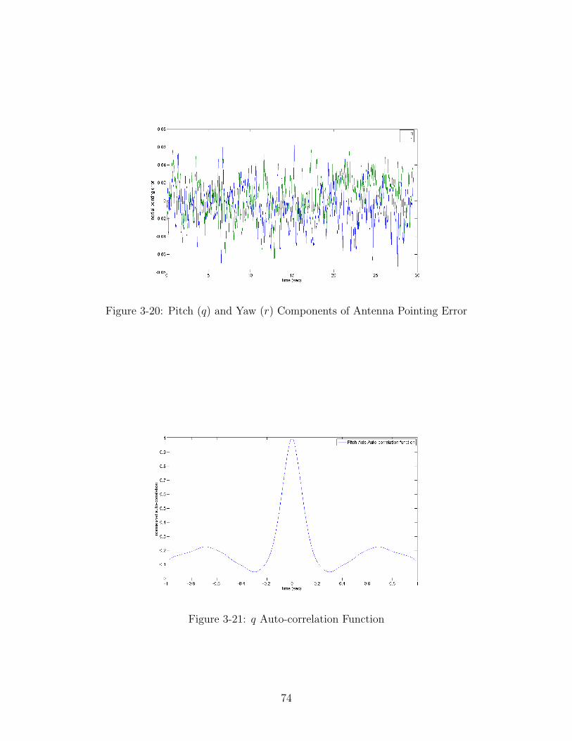
Figure 3-20: Pitch (q) and Yaw (r) Components of Antenna Pointing Error
Figure 3-21: q Auto-correlation Function
74
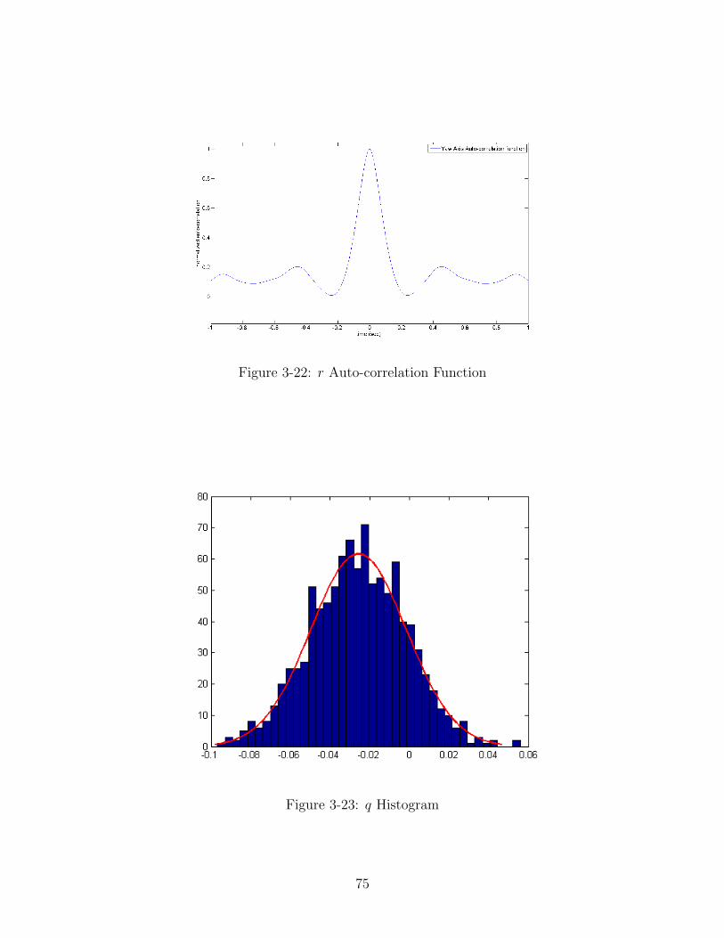
Figure 3-22: r Auto-correlation Function
Figure 3-23: q Histogram
75
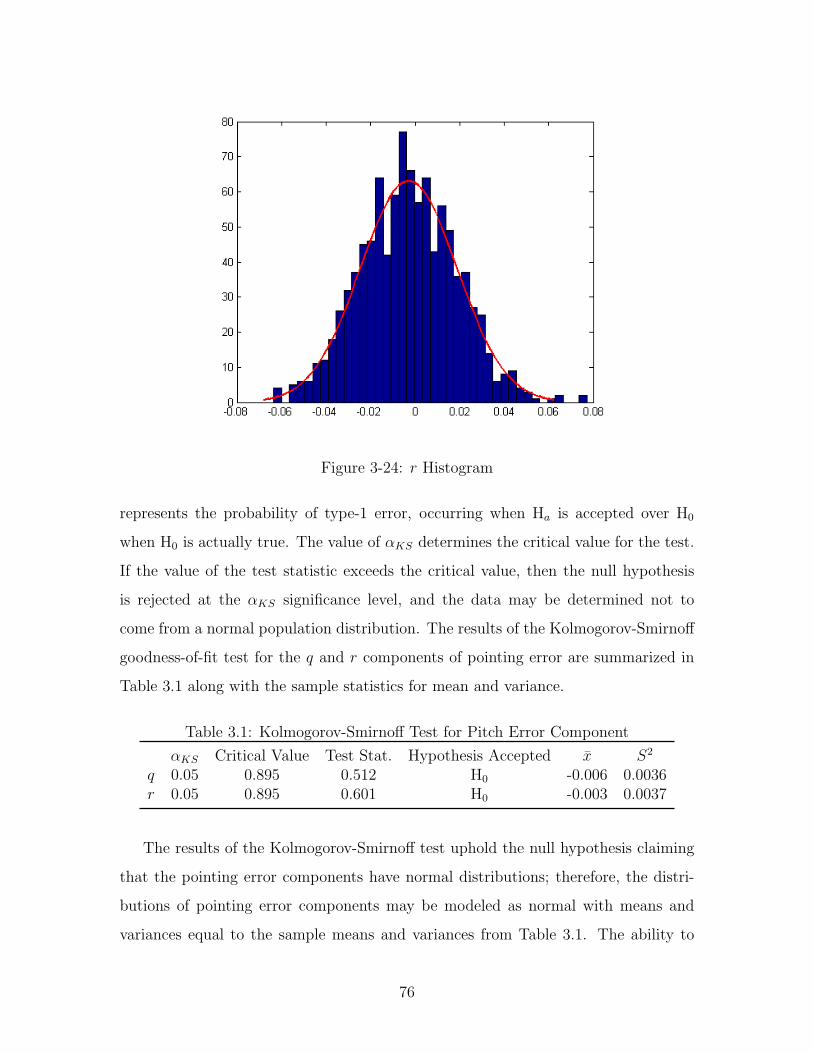
Figure 3-24: r Histogram
represents the probability of type-1 error, occurring when Ha is accepted over H0
when H0 is actually true. The value of αKS determines the critical value for the test.
If the value of the test statistic exceeds the critical value, then the null hypothesis
is rejected at the αKS significance level, and the data may be determined not to
come from a normal population distribution. The results of the Kolmogorov-Smirnoff
goodness-of-fit test for the q and r components of pointing error are summarized in
Table 3.1 along with the sample statistics for mean and variance.
Table 3.1: Kolmogorov-Smirnoff Test for Pitch Error Component
αKS Critical Value Test Stat. Hypothesis Accepted x S2
q 0.05 0.895 0.512 H0 -0.006 0.0036r 0.05 0.895 0.601 H0 -0.003 0.0037
The results of the Kolmogorov-Smirnoff test uphold the null hypothesis claiming
that the pointing error components have normal distributions; therefore, the distri-
butions of pointing error components may be modeled as normal with means and
variances equal to the sample means and variances from Table 3.1. The ability to
76

approximate the pointing error components as normally distributed assists in the
modeling and simulation of closed-loop step-tracking algorithms developed in the
next chapter.
77

78

Chapter 4
Closed-Loop Pointing Strategy
Overview
Because the nominal APS defined in Section 2.3 attempts to minimize inertial mis-
pointing with the simplest available system, step-tracking is the closed-loop strategy
that will be implemented with the nominal APS and open-loop feedback controller
developed in the previous chapter. The resulting pointing strategy is classified as
hybrid open/closed-loop in the sense that the closed-loop step-tracking algorithm up-
dates the reference commands to the open-loop pedestal controller. The antenna’s
gain pattern will be defined as a nonlinear, scalar cost function that the step-tracking
algorithms developed in this chapter must optimize. Step-tracking algorithms accom-
plish both spatial pull-in and closed-loop tracking by optimizing the antenna’s gain
pattern.
Five step-tracking algorithms will be tested through simulation in terms of how
well each algorithm accomplishes spatial pull-in with various initial pointing errors.
Next, selected step-tracking algorithms will be tested through simulation under con-
ditions simulating harsher inertial open-loop pointing error and satellite motion. Fi-
nally, the best performing algorithm in the simulated spatial pull-in tests will undergo
simulated closed-loop tracking tests of a target satellite. The results of each of the
simulations will be used to gauge the feasibility of using step-tracking algorithms as
a closed-loop pointing strategy for an airborne EHF SATCOM application.
79
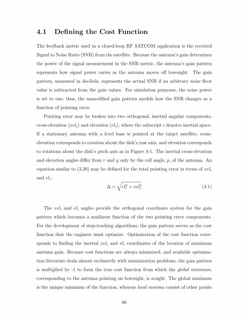
4.1 Defining the Cost Function
The feedback metric used in a closed-loop RF SATCOM application is the received
Signal to Noise Ratio (SNR) from the satellite. Because the antenna’s gain determines
the power of the signal measurement in the SNR metric, the antenna’s gain pattern
represents how signal power varies as the antenna moves off boresight. The gain
pattern, measured in decibels, represents the actual SNR if an arbitrary noise floor
value is subtracted from the gain values. For simulation purposes, the noise power
is set to one; thus, the unmodified gain pattern models how the SNR changes as a
function of pointing error.
Pointing error may be broken into two orthogonal, inertial angular components,
cross-elevation (xeli) and elevation (eli), where the subscript i denotes inertial space.
If a stationary antenna with a level base is pointed at the target satellite, cross-
elevation corresponds to rotation about the dish’s yaw axis, and elevation corresponds
to rotations about the dish’s pitch axis as in Figure 4-1. The inertial cross-elevation
and elevation angles differ from r and q only by the roll angle, p, of the antenna. An
equation similar to (3.20) may be defined for the total pointing error in terms of xeli
and eli:
∆ =√el2i + xel2i (4.1)
The xeli and eli angles provide the orthogonal coordinate system for the gain
pattern which becomes a nonlinear function of the two pointing error components.
For the development of step-tracking algorithms, the gain pattern serves as the cost
function that the engineer must optimize. Optimization of the cost function corre-
sponds to finding the inertial xeli and eli coordinates of the location of maximum
antenna gain. Because cost functions are always minimized, and available optimiza-
tion literature deals almost exclusively with minimization problems, the gain pattern
is multiplied by -1 to form the true cost function from which the global minimum,
corresponding to the antenna pointing on boresight, is sought. The global minimum
is the unique minimum of the function, whereas local minima consist of other points
80
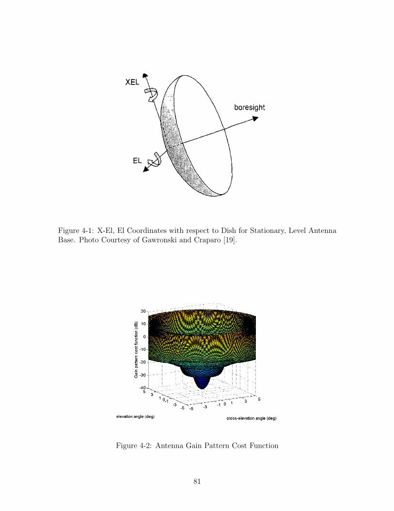
Figure 4-1: X-El, El Coordinates with respect to Dish for Stationary, Level AntennaBase. Photo Courtesy of Gawronski and Craparo [19].
Figure 4-2: Antenna Gain Pattern Cost Function
81
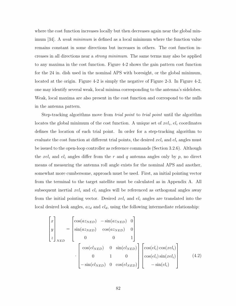
where the cost function increases locally but then decreases again near the global min-
imum [34]. A weak minimum is defined as a local minimum where the function value
remains constant in some directions but increases in others. The cost function in-
creases in all directions near a strong minimum. The same terms may also be applied
to any maxima in the cost function. Figure 4-2 shows the gain pattern cost function
for the 24 in. dish used in the nominal APS with boresight, or the global minimum,
located at the origin. Figure 4-2 is simply the negative of Figure 2-3. In Figure 4-2,
one may identify several weak, local minima corresponding to the antenna’s sidelobes.
Weak, local maxima are also present in the cost function and correspond to the nulls
in the antenna pattern.
Step-tracking algorithms move from trial point to trial point until the algorithm
locates the global minimum of the cost function. A unique set of xeli, eli coordinates
defines the location of each trial point. In order for a step-tracking algorithm to
evaluate the cost function at different trial points, the desired xeli and eli angles must
be issued to the open-loop controller as reference commands (Section 3.2.6). Although
the xeli and eli angles differ from the r and q antenna angles only by p, no direct
means of measuring the antenna roll angle exists for the nominal APS and another,
somewhat more cumbersome, approach must be used. First, an initial pointing vector
from the terminal to the target satellite must be calculated as in Appendix A. All
subsequent inertial xeli and eli angles will be referenced as orthogonal angles away
from the initial pointing vector. Desired xeli and eli angles are translated into the
local desired look angles, azd and eld, using the following intermediate relationship:x
y
z
NED
=
cos(azNED) − sin(azNED) 0
sin(azNED) cos(azNED) 0
0 0 1
·
cos(elNED) 0 sin(elNED)
0 1 0
− sin(elNED) 0 cos(elNED)
cos(eli) cos(xeli)
cos(eli) sin(xeli)
− sin(eli)
(4.2)
82
where azNED and elNED are the inertial look angles in the North, East, Down Co-
ordinate Frame (Appendix A). Equation (4.2) develops a pointing vector in the
topocentric North, East, Down inertial frame from which the local desired look an-
gles, azd and eld, are calculated from Equations (A.1), (A.2), and (A.11). Reference
commands from a closed-loop step-tracking algorithm may now be issued to the open-
loop pedestal controller forming the hybrid open/closed-loop pointing strategy.
4.2 Facets of the Optimization Problem
Several issues arise when one applies step-tracking algorithms as a closed-loop an-
tenna pointing solution for a mobile SATCOM application. First, only the function
values of the cost function in Figure 4-2 may be obtained by measuring the SNR as the
antenna points at a particular xeli, eli coordinate. Any gradient or second-derivative
measurements of the cost function must be approximated using finite differencing.
Thus, optimization methods requiring cost function derivatives at a particular trial
point mandate cost function evaluations at additional surrounding trial points, and
the algorithm becomes more computationally expensive. Secondly, in real SATCOM
terminal systems, the SNR measurement may only be meaningfully computed to a
resolution of approximately 0.1 dB. This limitation has significant implications for
selecting an appropriate finite differencing interval and restricts the obtainable accu-
racy of cost function optimization. Thirdly, the cost function possesses multiple weak
maxima and minima, corresponding to sidelobes and nulls present in the antenna gain
pattern, that make the optimization difficult as these points must be distinguished
from the global minimum. Fourthly, the pointing error from the open-loop pedestal
controller and the noise within the terminal system make SNR measurements, and
therefore the cost function, stochastic. At each trial point visited, the stare time
must be made long enough to average the effects of both of these noise sources [11].
Stare time is the time spent averaging the SNR measurements at each inertial xeli, eli
coordinate that the step-tracking algorithm visits. Although terminal system noise
contributes to the required stare time, all closed-loop pointing strategies must in-
83
corporate stare times for obtaining accurate SNR measurements in the presence of
system noise. Therefore, the effects of terminal system noise are not incorporated
in the spatial pull-in and tracking simulations discussed in this chapter because the
presence of system noise neither adds to nor detracts from the feasibility of using
step-tracking algorithms for mobile SATCOM applications. Lastly, due to the mo-
tion of the aircraft and slowly time varying sources of error identified in Section 2.2.1,
the satellite appears as a slowly moving target in inertial space, and the cost function
develops time dependencies as well. Step-tracking algorithms must account for the
apparent motion of the satellite during both the spatial pull-in stage and the tracking
stage and must be robust enough to optimize a slowly time varying, stochastic cost
function. Step-tracking systems must deal with all of these issues accordingly in order
to successfully accomplish closed-loop antenna pointing.
Step-tracking algorithms must optimize the gain pattern cost function while min-
imizing the computational expense incurred by the algorithm. In step-tracking algo-
rithms, excessive SNR measurements add to the computational expense metric and
detract from the convergence time, or the time it takes the step-tracking algorithm
to locate the minimum of the cost function. SNR measurements, or cost function
evaluations, are much more computationally expensive than the overhead of the step-
tracking algorithm, particularly when the number of independent variables that define
the cost function is small [34]. Consequently, overhead times will be ignored in the
performance comparisons of step-tracking algorithms developed in this chapter as the
gain pattern cost function is defined by only two independent variables.
4.3 Step-tracking Using Function Comparison Meth-
ods
4.3.1 Full-field Search
A full-field function comparison search constitutes the simplest method of step-
tracking. Function comparison methods work by measuring the cost function at
84
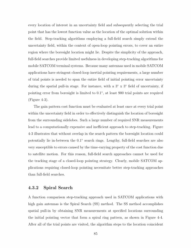
every location of interest in an uncertainty field and subsequently selecting the trial
point that has the lowest function value as the location of the optimal solution within
the field. Step-tracking algorithms employing a full-field search simply extend the
uncertainty field, within the context of open-loop pointing errors, to cover an entire
region where the boresight location might lie. Despite the simplicity of the approach,
full-field searches provide limited usefulness in developing step-tracking algorithms for
mobile SATCOM terminal systems. Because many antennas used in mobile SATCOM
applications have stringent closed-loop inertial pointing requirements, a large number
of trial points is needed to span the entire field of initial pointing error uncertainty
during the spatial pull-in stage. For instance, with a 3 x 3 field of uncertainty, if
pointing error from boresight is limited to 0.1, at least 900 trial points are required
(Figure 4-3).
The gain pattern cost function must be evaluated at least once at every trial point
within the uncertainty field in order to effectively distinguish the location of boresight
from the surrounding sidelobes. Such a large number of required SNR measurements
lead to a computationally expensive and inefficient approach to step-tracking. Figure
4-3 illustrates that without overlap in the search pattern the boresight location could
potentially lie in-between the 0.1 search rings. Lengthy, full-field searches are also
very susceptible to errors caused by the time-varying property of the cost function due
to satellite motion. For this reason, full-field search approaches cannot be used for
the tracking stage of a closed-loop pointing strategy. Clearly, mobile SATCOM ap-
plications requiring closed-loop pointing necessitate better step-tracking approaches
than full-field searches.
4.3.2 Spiral Search
A function comparison step-tracking approach used in SATCOM applications with
high gain antennas is the Spiral Search (SS) method. The SS method accomplishes
spatial pull-in by obtaining SNR measurements at specified locations surrounding
the initial pointing vector that form a spiral ring pattern, as shown in Figure 4-4.
After all of the trial points are visited, the algorithm steps to the location coincident
85
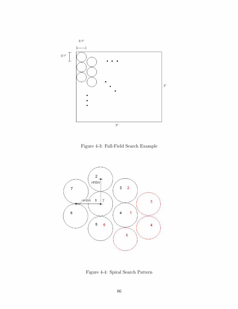
Figure 4-3: Full-Field Search Example
Figure 4-4: Spiral Search Pattern
86
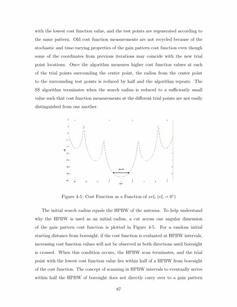
with the lowest cost function value, and the test points are regenerated according to
the same pattern. Old cost function measurements are not recycled because of the
stochastic and time-varying properties of the gain pattern cost function even though
some of the coordinates from previous iterations may coincide with the new trial
point locations. Once the algorithm measures higher cost function values at each
of the trial points surrounding the center point, the radius from the center point
to the surrounding test points is reduced by half and the algorithm repeats. The
SS algorithm terminates when the search radius is reduced to a sufficiently small
value such that cost function measurements at the different trial points are not easily
distinguished from one another.
Figure 4-5: Cost Function as a Function of xeli (eli = 0)
The initial search radius equals the HPBW of the antenna. To help understand
why the HPBW is used as an initial radius, a cut across one angular dimension
of the gain pattern cost function is plotted in Figure 4-5. For a random initial
starting distance from boresight, if the cost function is evaluated at HPBW intervals,
increasing cost function values will not be observed in both directions until boresight
is crossed. When this condition occurs, the HPBW scan terminates, and the trial
point with the lowest cost function value lies within half of a HPBW from boresight
of the cost function. The concept of scanning in HPBW intervals to eventually arrive
within half the HPBW of boresight does not directly carry over to a gain pattern
87
cost function defined by two independent variables (xeli and eli); however, a spiral
search method with an initial radius equal to a HPBW does locate the mainlobe of
the gain pattern cost function a large percentage of the time. The SS step-tracking
algorithm typically converges on boresight quickly, for cases when it does converge.
The same SS algorithm used for spatial pull-in cannot be used for tracking because
the first few spiral search radii are large, and the process would dither the antenna
an unacceptable distance away from boresight. The non-convergence issues inherent
in the SS method may also make it a less attractive option for accomplishing spatial
pull-in. Because of the pitfalls inherent in the SS step-tracking algorithm, a more
robust method is desired which may also be used for closed-loop tracking.
4.4 Step-tracking Using Optimization Techniques
By applying nonlinear function optimization methods to the gain pattern cost func-
tion, one may develop reliable step-tracking methods capable of accomplishing both
spatial pull-in and closed-loop tracking. Optimization methods for nonlinear functions
are iterative algorithms that move from trial point to trial point in the n-dimensional
space spanned by the cost function until the termination conditions for the algorithm
are met (if termination conditions exist). If the cost function is a function of n inde-
pendent variables, then x is a size-n position vector specifying the location in n-space
of the trial point. For step-tracking algorithms using optimization methods, x is a
2x1 vector containing the xeli and eli orthogonal inertial pointing angles. In general,
optimization methods must satisfy
Fk+1 ≤ Fk (4.3)
where Fk is the cost function evaluated at the k-th iteration of the algorithm [34].
Equation (4.3) ensures that each iteration of the optimization algorithm produces a
successively smaller value of the cost function. Nonlinear cost function optimization
88
algorithms follow the update formula
xk+1 = xk + αpk (4.4)
where xk+1 is the next trial point location where the cost function is to be evaluated,
xk is the current location, pk is a descent direction, and α is the step length taken in
the descent direction [34–36]. Descent directions must follow a direction of negative
curvature in the cost function, meeting the stipulation
pTkGkpk ≤ 0 (4.5)
where Gk is the second-derivative Hessian matrix of the cost function at the k-th trial
point [34–36]. The specific optimization approach applied determines the descent
direction in Equation (4.4). The value of α in Equation (4.4) specifies how far the
algorithm should travel along the descent direction and is determined by a linear
search procedure.
The terminal conditions for optimization methods must be carefully defined for
the specific application. For step-tracking applications accomplishing spatial pull-in,
the algorithm must locate the global minimum corresponding to the inertial angular
coordinates of boresight. At boresight, or the peak of the mainlobe of the gain pattern,
the gradient of the cost function vanishes; however, the gradient is also equal to zero at
the weak minimums of the cost function where the sidelobes in the gain pattern occur.
To effectively accomplish spatial pull-in, the algorithm must not terminate until the
gradient is sufficiently close to zero and the minimum has been determined to be a
strong one. Although the gain pattern cost function contains weak maxima, where the
nulls in the gain pattern occur, the gradient values at these points cannot be precisely
calculated because of the sharpness of the cost function at the nulls. As such, the
weak maxima in the cost function do not have zero gradient values and do not pose
potential termination points for step-tracking algorithms accomplishing spatial pull-
in. Step-tracking systems may accomplish closed-loop tracking by eliminating the
terminal conditions imposed in the spatial pull-in stage and running the optimization
89
algorithm in an infinite loop. Tracking may also be accomplished by scheduling the
same algorithm used in the spatial pull-in stage to run at regular intervals or at times
when the strength of the SATCOM link has been sufficiently degraded.
Optimization methods applied to nonlinear cost functions seek to achieve the
highest possible asymptotic rate of convergence. An optimization algorithm asymp-
totically converges on the desired solution with order o, where o is the largest number
such that
0 ≤ limk→∞
||xk+1 − x∗||||xk − x∗||o
≤ ∞ (4.6)
where x∗ is the global minimum of the cost function. In practice, the best convergence
rate that is generally attainable is quadratic convergence, where o in (4.6) equals two,
so optimization literature emphasizes methods that exhibit this property [34,36].
4.4.1 Modified Newton’s Method
The first optimization method applied to the development of step-tracking algorithms
is a Modified Newton’s (MN) method. The precepts behind Newton’s method stem
from optimization techniques applied to quadratic cost functions. A generic quadratic
cost function may be written as
F (x) =1
2xTAx + bTx + c (4.7)
where A must be a symmetric matrix [34]. The gradient and second-derivatives of
the function in (4.7) may be calculated using Equations (4.8) and (4.9).
g(x) = Ax + b (4.8)
G(x) = A (4.9)
In Equations (4.8) and (4.9), g is the gradient vector and G is the second-derivative
Hessian matrix. For a quadratic cost function, the exact Taylor series expansion of
90
the gradient at the next trial point, xk+1, may be written as
gk+1 = gk +Gpk (4.10)
where all higher derivatives are zero for quadratic cost functions [34]. If xk+1 is to
be the minimum of the quadratic cost function, Equation (4.10) must equal zero.
Newton’s method algorithms subsequently determine a descent direction for use in
Equation (4.4) according to
pk = −G−1gk (4.11)
where gk is the cost function gradient at the current trial point and G is the Hessian
matrix of the assumed quadratic cost function [34–36]. Equation (4.11) exactly de-
termines the minimum of a quadratic function in a single iteration. On non-quadratic
functions, the process repeats iteratively until the minimum is found according to
pk = −G−1k gk (4.12)
where Gk is now the Hessian matrix at the given trial point.
Newton’s method generally exhibits quadratic convergence rates making it a viable
approach for minimizing nonlinear cost functions [36]. Difficulties with the approach
in (4.12) arise when Gk is not positive definite and actual descent directions are not
generated; i.e. the pk vector generated by (4.12) does not satisfy (4.5). Modified
Newton’s Methods solve this problem by altering the Hessian matrix, Gk, to ensure
that it is as close to the original Gk matrix as possible, yet sufficiently positive defi-
nite. One of the best approaches to modifying the Gk matrix employs the Cholesky
Factorization described in Equations (4.13)-(4.14) [34–36].
91
Gk = LkDkLTk (4.13)
djj = gjj −j−1∑q=1
dqql2jq (4.14)
lij = (gij −j−1∑q=1
dqqliqljq)/djj i = j + 1, j + 2, . . . , n (4.15)
where gij, lij, and dij are the elements of Gk, Lk, and Dk respectively and j =
1, 2, . . . , n. If Gk is positive definite, then the diagonal Dk matrix in (4.13) will have
positive entries. If any of the elements of the Dk matrix are less than an arbitrarily
small positive number, δG, then Gk is replaced by Gk given by
Gk = LkDkLTk (4.16)
djj = gjj + rjj −j−1∑q=1
dqq l2jq = δG (4.17)
lij = (gij −j−1∑q=1
dqq liq ljq)/djj i = j + 1, j + 2, . . . , n (4.18)
(4.19)
where rjj is the amount added to the diagonal values of D to ensure they are greater
than or equal to δG and j again increments column-wise from 1 to n [34]. Gk becomes
the modified approximation to the Hessian matrix at the given trial point and is
related to the original approximation by Gk = Gk + Rk where Rk is a diagonal
matrix containing the rjj values. Because Gk is sufficiently positive definite, a descent
direction that satisfies (4.5) may now be found by solving Equation (4.20).
pk = −G−1gk (4.20)
The value of δG places a lower limit on the “positive definiteness” requirement of Gk.
The δG value is rarely equal to zero to account for errors in the computation and/or
approximation of the Hessian matrix. A selection of δG = 10 is used in the modified
Newton step-tracking simulations developed in this chapter with good results.
92
4.4.2 Quasi-Newton’s Methods
Quasi-Newton methods attempt to optimize nonlinear cost functions without the use
of second-derivatives while maintaining quadratic convergence rates. Quasi-Newton
Methods determine the descent direction according to:
Bkpk = −gk (4.21)
Bk+1 = Bk +Qk (4.22)
where Bk in some way approximates Gk from (4.12), and Qk is an update matrix de-
pendent upon xk, xk+1, gk, and gk+1 [34–36]. In the absence of additional knowledge
about the cost function, B0 may be initialized to the identity matrix [34, 36]. Bk+1
must also satisfy the quasi-Newton Condition that ρkBk+1∆xk = ∆gk [35]. The value
of the constant, ρk, is normally set to unity which forces the Bk+1 matrix to have
the same curvature information as the second-derivative matrix in the pk direction
for quadratic cost functions [34]. As the quasi-Newton algorithm iterates, and a cost
function minima is neared, Bk becomes a successively better approximation to Gk.
Two separate methods for calculating the update matrix, Qk, in Equation (4.22)
are applied to developing step-tracking algorithms in this chapter; the method of
Davidon, Fletcher, and Powell (DFP) and the method of Broyden, Fletcher, Gold-
farb, and Shano (BFGS). The formula for the DFP and BFGS update matrices are
presented in Equations (4.23) and (4.24), respectively.
Qk = αgk∆gTk
∆gTk∆xk+ α
∆gkgTk
∆gTk∆xk− α∆gkg
Tk∆xk∆gTk
(∆gTk∆xk)2+
∆gk∆gTk∆gTk∆xk
(4.23)
Qk =∆gk∆gTk∆gTk∆xk
+ αgkg
Tk
∆xTk gk(4.24)
For derivations of the update formula in Equations (4.23)–(4.24), the reader is referred
to the literature [34–36]. In general, the BFGS method is purported to have much
better performance optimizing nonlinear functions than the DFP method [34], but
step-tracking algorithms using both methods will be developed and applied in this
chapter for comparison.
93
As in the modified Newton’s method, quasi-Newton’s methods only generate de-
scent directions when the Bk matrix in (4.21) is positive definite. The update formula
for both the DFP and BFGS methods are theoretically structured such that Bk re-
mains positive definite at each iteration of the optimization algorithm [34, 35]. In
spite of theoretical guarantees, Bk often tends to lose positive definiteness due to
rounding errors, particularly when cost function gradients are approximated using
finite differencing techniques (as is the case in step-tracking algorithms). To ensure
Bk remains positive definite, the step-tracking algorithms developed in this chapter
incorporate the same procedure outlined in Equations (4.16)-(4.18) for developing a
sufficiently positive definite version of Bk when necessary. The resulting Bk matrix,
similar to Gk in (4.16), is used to determine a descent direction according to (4.21)
where Bk is replaced by Bk.
4.4.3 Method of Steepest Descent
The simplest optimization method to develop step-tracking algorithms in this chapter
is the method of Steepest Descent (SD). The SD method simply sets the descent
direction equal to the negative of the cost function gradient at the current trial point
according to Equation (4.25).
pk = −gk (4.25)
Steepest Descent algorithms rely more heavily on accurate linear searches to deter-
mine the step length in Equation (4.4) than the Newton methods do. Accurate linear
searches greatly increase the number of cost function evaluations accomplished per
major algorithm iteration; an effect that is generally undesirable for applications re-
quiring quick convergence. Steepest Descent methods exhibit only linear convergence
rates but are very stable and less complex than other optimization techniques [34].
Because of the radial nature of the gain pattern cost function, SD optimization al-
gorithms should produce descent directions which are tangent to the contours of the
cost function; thus, boresight of the cost function could theoretically be found in one
major algorithm iteration if the correct step length is determined. Because of the
94
potential for SD methods to easily optimize the gain pattern cost function without
the use of second-derivative approximations, a step-tracking algorithm using an SD
technique is developed in this chapter for comparison to the Newton methods.
4.4.4 Step-tracking Algorithm Architecture
The basic architecture described below produces step-tracking algorithms that accom-
plish closed-loop spatial pull-in of a target satellite using the methods of optimization
described in Sections 4.4.1–4.4.3. This architecture changes very little as a function of
optimization method. Major differences in step-tracking algorithms using optimiza-
tion techniques arise only in the approach used by each method to calculate pk in
Equation (4.4) (Line 24 of Algorithm 1).
Lines 1-3 initialize the terminal conditions, begin the while loop, and initialize the
logical variable that determines whether or not a descent direction and step-length are
calculated for this iteration (a predetermined αpk is calculated when the algorithm
is at a local minima; Lines 8,14). Line 4 computes the value of the cost function at
x as well as at any nearby points required to approximate first or second-derivatives
of the cost function. Lines 5-17 determine what procedures are accomplished by
the algorithm when a minimum has been reached. If the algorithm determines it is
currently at a local, weak minimum, Lines 6-10 instruct the algorithm to jump off of
the local minimum in the direction of the global minimum. If the algorithm thinks
it may have located the global minimum, lines 11-17 instruct the algorithm to repeat
itself, without changing the trial point location, a number of times equal to “mincheck
threshold” to make sure that the global minimum has actually been found; then the
terminal conditions are set to true. The stochastic nature of the cost function makes
this process necessary.
In the event that the repeated trial point is no longer close enough to the global
minimum, lines 18-20 reset to zero the number of times the algorithm has repeated
itself and instructs the algorithm to calculate αpk. This event can be thought of
as “falling off” of the global minimum, due to the time-varying nature of the cost
function. This can occur in the amount of time it takes the algorithm to repeat
95

Algorithm 1 Step-Tracking Algorithm using Function Optimization Methods
1: set terminate = false2: while terminate == false do3: set compute αpk = true4: perform function/gradient evaluations at xk5: if criteria for minimum == true (small gradient) then6: check for local min7: if local min == true then8: αpk = jump condition αpk9: mincheck = 0
10: else11: αpk = 012: mincheck = mincheck +113: end if14: compute αpk = false15: if mincheck > mincheck threshold then16: terminate=true17: end if18: else if mincheck > 0 && criteria for minimum ==false then19: mincheck = 020: compute αpk = true21: end if22:23: if compute αpk == true then24: compute pk and initial α25: limit αpk to a predetermined region of confidence26: perform linear search along pk to determine satisfactory α27: end if28: xk+1 = xk + αpk29: end while
96
itself to check if it is on the global minimum or not. Experience has shown that
the algorithm should only repeat itself once or twice at a single trial point while
checking the global minimum terminal conditions in order to avoid “falling off” the
global minimum during this time. Lines 23-27 determine a descent direction and a
step length and are only accomplished if the algorithm is not at a minima. Line
25 limits the initial step length to within some “region of confidence.” This step is
accomplished because many of the algorithms calculate very large initial step lengths
away from the current trial point when smaller ones are required. Finally, Line 28
determines the next trial point according to (4.4).
The step-tracking algorithms developed to accomplish spatial pull-in may be modi-
fied for use in closed-loop tracking by simply removing the terminal conditions. Track-
ing algorithms also do not require the weak versus strong minimum discrimination
procedure in Lines 5-21 because the strong minimum of the gain pattern cost function
has already been located in the spatial pull-in stage.
Finite Difference Approximations for First and Second-Derivatives
Line 4 in Algorithm 1 instructs the step-tracking method to approximate the required
first and second cost function derivatives. A standardized map of cost function eval-
uation locations relative to the current trial point, xk, is followed in each of the four
nonlinear optimization methods when gradients or second-derivatives must be approx-
imated. Figure 4-6 shows the cost function evaluation locations where the current
trial point is labeled point 1 and δf is the finite differencing interval chosen. Because
xeli together with eli and r together with q represent orthogonal components of iner-
tial pointing error, the pointing error distributions derived for r and q in Section 3.3
are applied as distribution models for xeli and eli. Consequently, the 3-σ value for the
open loop pointing error in the eli and xeli component directions is 0.06 (Sections
3.2.5 and 3.2.6). The finite differencing interval for each of the nonlinear optimiza-
tion algorithms is selected to be between 2-3 times larger than the 3-σ value for the
open-loop pointing error components in order to sufficiently distinguish cost function
values measured at different points on the function map in Figure 4-6 [36]. The finite
97
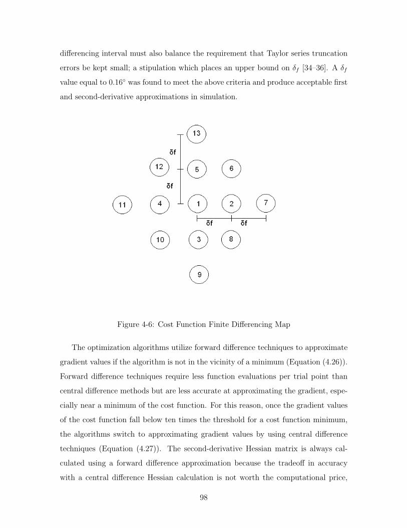
differencing interval must also balance the requirement that Taylor series truncation
errors be kept small; a stipulation which places an upper bound on δf [34–36]. A δf
value equal to 0.16 was found to meet the above criteria and produce acceptable first
and second-derivative approximations in simulation.
Figure 4-6: Cost Function Finite Differencing Map
The optimization algorithms utilize forward difference techniques to approximate
gradient values if the algorithm is not in the vicinity of a minimum (Equation (4.26)).
Forward difference techniques require less function evaluations per trial point than
central difference methods but are less accurate at approximating the gradient, espe-
cially near a minimum of the cost function. For this reason, once the gradient values
of the cost function fall below ten times the threshold for a cost function minimum,
the algorithms switch to approximating gradient values by using central difference
techniques (Equation (4.27)). The second-derivative Hessian matrix is always cal-
culated using a forward difference approximation because the tradeoff in accuracy
with a central difference Hessian calculation is not worth the computational price,
98
(4.28) [35]. Equation (4.29) ensures the approximation to the Hessian matrix satisfies
the symmetry property of second-derivative matrices [34–36].
gj(x) ≈ F (x + δfej)− F (x)
δf(4.26)
gj(x) ≈ F (x + δfej)− F (x− δfej)2δf
(4.27)
Gj =g(x + δfej)− g(x)
δf(4.28)
G ≈ 1
2(G + G
T) (4.29)
The subscript j in Equations (4.26)-(4.27) represents the j-th element of g while ej
represents the unit vector in the j-th direction. In Equation (4.28) the subscript j
represents the j-th column of the Hessian matrix approximation, G.
Minimum Discrimination
Lines 5-17 of Algorithm 1 check to see if the step-tracking algorithm has reached a
cost function minima and also determine whether or not that minima is the global
minimum. Each of the four nonlinear optimization algorithms use the same strategy
to move away from a weak, local minimum and to travel in the direction of the global
minimum. If the gradient is sufficiently small and the algorithm believes it has reached
a minimum, then the algorithm carries out the function evaluations necessary to
approximate the second-derivative Hessian matrix of the cost function at the current
trial point according to Equation (4.28). If the algorithm is at a weak minimum,
the approximation to the Hessian matrix should be nearly positive semi-definite.
At the strong minimum, the approximate Hessian matrix should be strongly positive
definite because the cost function has sufficient concavity in all directions. As a test for
positive definiteness in the Hessian matrix, the step-tracking algorithms determine the
Cholesky matrix factors of the G matrix as in Equations (4.13)-(4.15). If one or both
of the elements of the diagonal D matrix are less than some small positive, δG, then
the Hessian matrix lacks the required positive definiteness for a strong minimum [34],
and the algorithm determines that the current trial point is on a sidelobe of the gain
99
pattern cost function. A value of δG=10 is again used in simulation with good results
for weak minimum discrimination.
If the algorithm determines that it has reached a weak minimum, a specific update,
αpk, is used in Equation (4.4) to determine the location of the next trial point.
The two eigenvectors of the Hessian matrix point in the direction of maximum and
minimum curvature because the cost function is a function of only two independent
variables [34]. Because the gain pattern cost function is radially symmetric, and
the weak minima corresponding to antenna sidelobes circle the mainlobe, one of the
eigenvectors of the Hessian matrix points along the valley of the weak minimum
(direction of minimum curvature), and the other points orthogonal to it; i.e. either
toward boresight, or 180 away from boresight (direction of maximum curvature).
One may easily calculate a numeric value for the cost function curvature in the
direction of each eigenvector by calculating vTj Gvj where vj is the j-th eigenvector
of the Hessian matrix. Therefore, if the eigenvectors of the approximate Hessian are
calculated, and the direction of maximum curvature is found, the descent direction
may be taken as either vmax or −vmax where vmax is the eigenvector corresponding to
the direction of maximum curvature. Next, a step length value, α, must be calculated.
The value of the step length used in Equation (4.4) when the algorithm is at a weak
minimum is 1.85, the average peak to peak distance beginning at the mainlobe and
extending to the fourth sidelobe of the antenna gain pattern. Because the distance
between the sidelobes in the gain pattern is a function of HPBW, the α = 1.85 rule
changes dependent upon the HPBW of the given antenna. In order to determine
whether vj or −vmax is the appropriate descent direction, one must evaluate the cost
function at F (xk + 1.85vmax) and compare the measurement to F (xk). If the cost
function is higher at F (xk+1.85vmax) then the appropriate descent direction is −vmax;
whereas, if the cost function is lower, then vj should be taken as the descent direction.
Linear Search
Once the descent direction is calculated in Line 24 of Algorithm 1, its magnitude is
restricted to within a specified “region of confidence” for trial points not located at a
100
minima in the gain pattern cost function (Line 25) [35]. The region of confidence for
the step-tracking application is set to |pk| < 1. The 1 region of confidence prevents
the nonlinear optimization algorithms from jumping over nearby local maximas as
they progress into the valleys of the gain pattern cost function. Without the 1
restriction, the possibility exists for a wrong-way jump from one local maxima over
the next local maxima resulting in a descent into a sidelobe valley that is even farther
away from boresight. Because the distance between the nulls in the gain pattern cost
function is a function of HPBW, the 1 region of confidence varies with the HPBW
of the given antenna. After the conditional restriction on |pk| is applied, Line 26
calculates the desired step length along the descent direction according to a linear
search procedure. An appropriate step length will sufficiently reduce the directed
gradient of the cost function along the descent direction [34–36]. The directed gradient
measures the steepness of the cost function along a certain direction. If gradient values
are explicitly available, the criterion for a linear search is described by
|g(xk + αpk)Tpk| ≤ −ηgTkpk (4.30)
where 0 ≤ η < 1 and is called the linear search parameter. When η equals 0, the
directed gradient at xk + αpk must equal zero, and an exact linear search is carried
out. Accurate linear searches are typically computationally wasteful; therefore, values
of η > 0 are chosen for most nonlinear optimization algorithms [34,35]. If the gradient
values are not available, and are instead calculated by finite differencing, the criterion
in Equation (4.30) for the reduction of the directed gradient may be modified to
|F (xk + αpk)− F (xk + νpk)|δf
≤ −ηgTkpk (4.31)
where ν is the multiplier that satisfies |xk + αpk| − |xk + νpk| = δf [35].
The MN, BFGS, DFP, and SD algorithms implement the linear search in two steps.
First, the algorithm brackets an interval containing a minimum along the descent
direction, and secondly, the algorithm solves for the step length using a quadratic
polynomial interpolation procedure. In order to bracket a minimum along the descent
101
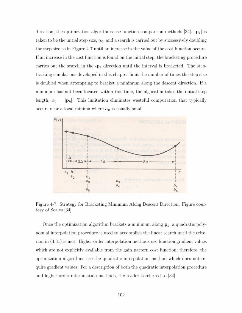
direction, the optimization algorithms use function comparison methods [34]. |pk| is
taken to be the initial step size, α0, and a search is carried out by successively doubling
the step size as in Figure 4-7 until an increase in the value of the cost function occurs.
If an increase in the cost function is found on the initial step, the bracketing procedure
carries out the search in the -pk direction until the interval is bracketed. The step-
tracking simulations developed in this chapter limit the number of times the step size
is doubled when attempting to bracket a minimum along the descent direction. If a
minimum has not been located within this time, the algorithm takes the initial step
length, α0 = |pk|. This limitation eliminates wasteful computation that typically
occurs near a local minima where α0 is usually small.
Figure 4-7: Strategy for Bracketing Minimum Along Descent Direction. Figure cour-tesy of Scales [34].
Once the optimization algorithm brackets a minimum along pk, a quadratic poly-
nomial interpolation procedure is used to accomplish the linear search until the crite-
rion in (4.31) is met. Higher order interpolation methods use function gradient values
which are not explicitly available from the gain pattern cost function; therefore, the
optimization algorithms use the quadratic interpolation method which does not re-
quire gradient values. For a description of both the quadratic interpolation procedure
and higher order interpolation methods, the reader is referred to [34].
102
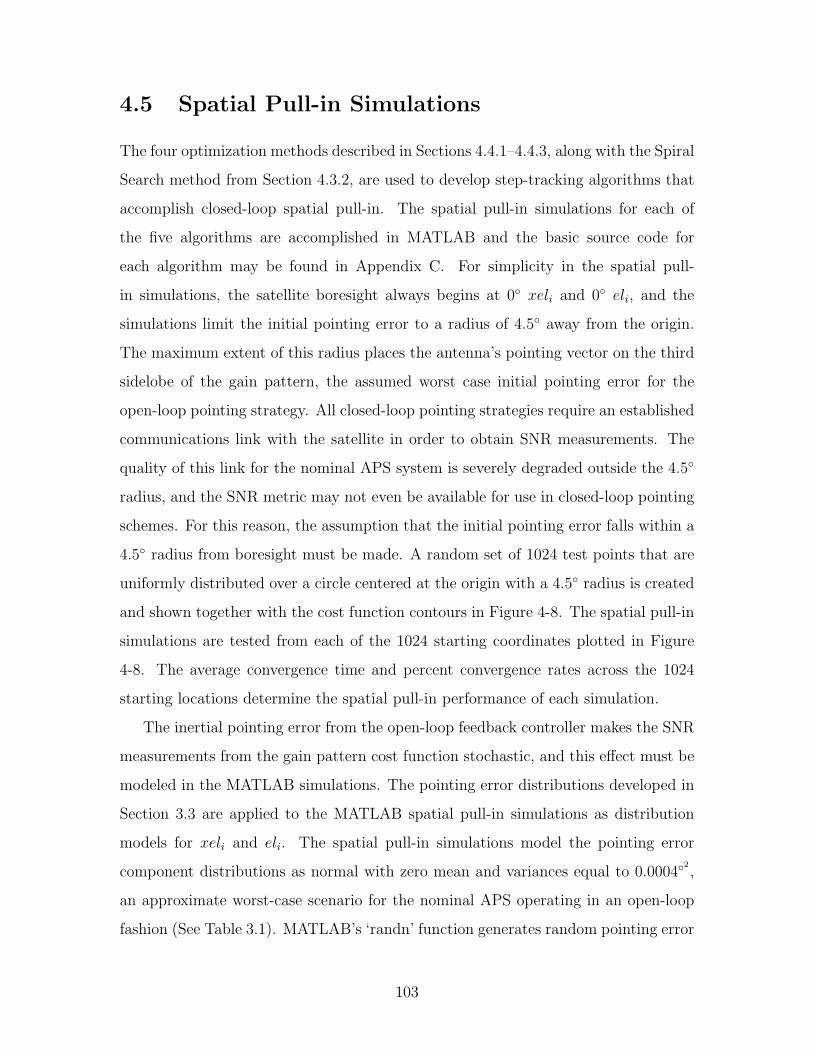
4.5 Spatial Pull-in Simulations
The four optimization methods described in Sections 4.4.1–4.4.3, along with the Spiral
Search method from Section 4.3.2, are used to develop step-tracking algorithms that
accomplish closed-loop spatial pull-in. The spatial pull-in simulations for each of
the five algorithms are accomplished in MATLAB and the basic source code for
each algorithm may be found in Appendix C. For simplicity in the spatial pull-
in simulations, the satellite boresight always begins at 0 xeli and 0 eli, and the
simulations limit the initial pointing error to a radius of 4.5 away from the origin.
The maximum extent of this radius places the antenna’s pointing vector on the third
sidelobe of the gain pattern, the assumed worst case initial pointing error for the
open-loop pointing strategy. All closed-loop pointing strategies require an established
communications link with the satellite in order to obtain SNR measurements. The
quality of this link for the nominal APS system is severely degraded outside the 4.5
radius, and the SNR metric may not even be available for use in closed-loop pointing
schemes. For this reason, the assumption that the initial pointing error falls within a
4.5 radius from boresight must be made. A random set of 1024 test points that are
uniformly distributed over a circle centered at the origin with a 4.5 radius is created
and shown together with the cost function contours in Figure 4-8. The spatial pull-in
simulations are tested from each of the 1024 starting coordinates plotted in Figure
4-8. The average convergence time and percent convergence rates across the 1024
starting locations determine the spatial pull-in performance of each simulation.
The inertial pointing error from the open-loop feedback controller makes the SNR
measurements from the gain pattern cost function stochastic, and this effect must be
modeled in the MATLAB simulations. The pointing error distributions developed in
Section 3.3 are applied to the MATLAB spatial pull-in simulations as distribution
models for xeli and eli. The spatial pull-in simulations model the pointing error
component distributions as normal with zero mean and variances equal to 0.00042,
an approximate worst-case scenario for the nominal APS operating in an open-loop
fashion (See Table 3.1). MATLAB’s ‘randn’ function generates random pointing error
103
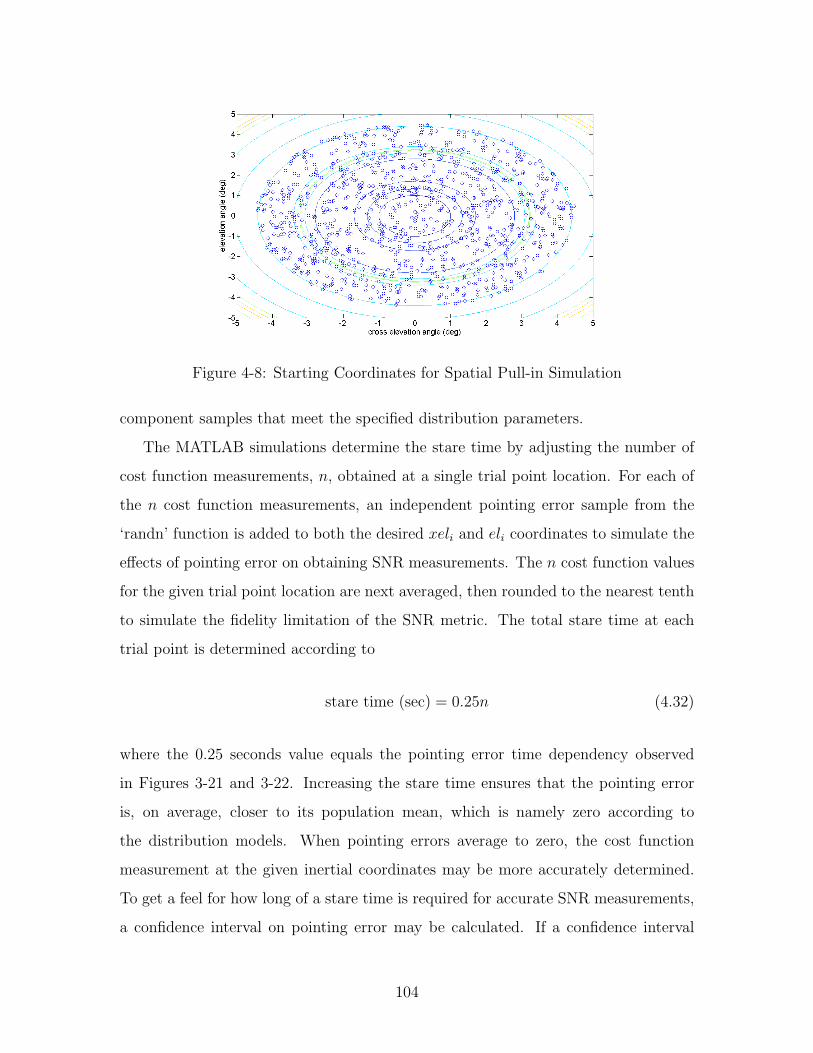
Figure 4-8: Starting Coordinates for Spatial Pull-in Simulation
component samples that meet the specified distribution parameters.
The MATLAB simulations determine the stare time by adjusting the number of
cost function measurements, n, obtained at a single trial point location. For each of
the n cost function measurements, an independent pointing error sample from the
‘randn’ function is added to both the desired xeli and eli coordinates to simulate the
effects of pointing error on obtaining SNR measurements. The n cost function values
for the given trial point location are next averaged, then rounded to the nearest tenth
to simulate the fidelity limitation of the SNR metric. The total stare time at each
trial point is determined according to
stare time (sec) = 0.25n (4.32)
where the 0.25 seconds value equals the pointing error time dependency observed
in Figures 3-21 and 3-22. Increasing the stare time ensures that the pointing error
is, on average, closer to its population mean, which is namely zero according to
the distribution models. When pointing errors average to zero, the cost function
measurement at the given inertial coordinates may be more accurately determined.
To get a feel for how long of a stare time is required for accurate SNR measurements,
a confidence interval on pointing error may be calculated. If a confidence interval
104
width of 0.02 is desired for each of the inertial pointing error components, at the
95% confidence level, Equation (4.33) reveals that a sample size of 16 independent
pointing error samples is required corresponding to a stare time of 4 seconds per trial
point location, according to Equation (4.32). The spatial pull-in performance of each
of the algorithms is examined for different stare times to see how the performance
changes as a function of the stare time parameter.
nCI =
(2zα
2S
wCI
)2
(4.33)
In Equation (4.33) nCI is the number of independent pointing error samples required
corresponding to the number of cost function evaluations conducted per trial point
(n). zα2
is the critical value from the normal distribution corresponding to the given
confidence interval, S is the standard deviation of the population, and w is the desired
confidence interval width [37].
Because of the motion of the aircraft, the gain pattern cost function translates in
the inertial reference frame defined by the cross-elevation and elevation axes. Figure
4-9 plots the magnitude of a geostationary target satellite’s inertial angular velocity
for a typical 707 flight profile. Some of the errors outlined in Section 2.2.1 also cause
slowly time varying errors that can be simulated by translating the cost function at
a certain velocity in the xeli, eli plane. The total translation of the cost function
in the spatial pull-in simulations is approximated by the maximum target satellite
velocity from Figure 4-9 plus an additional amount used to approximate time varying
pointing errors. The spatial pull-in simulations use a value of 0.0005
secfor the total
translational velocity of the cost function (vpat). In the MATLAB simulation, the cost
function translates equally in the negative xeli and eli directions for the duration of
the simulation which has the largest impact on the performance of step-tracking
algorithms.
Figures 3-17 and 3-18 show that the step response rise time between two iner-
tial coordinates is 0.25 seconds, which conveniently equals the elapsed time between
cost function measurements taken at a single xeli, eli point when stare times are
105
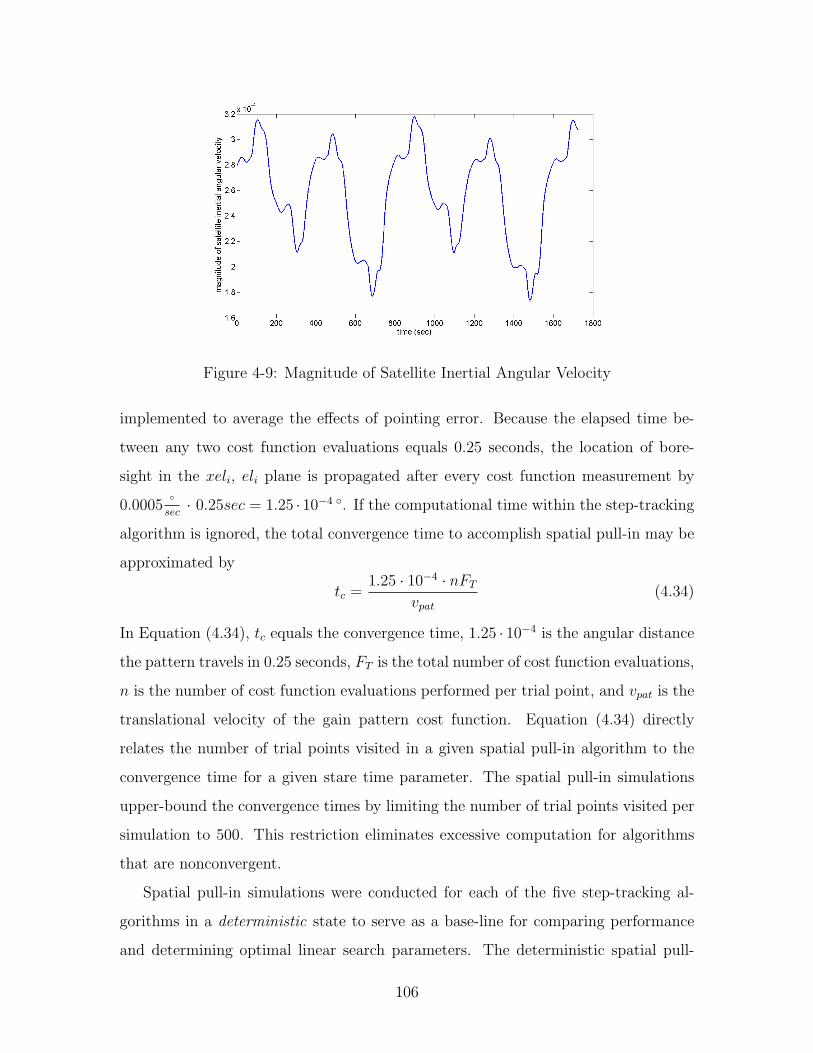
Figure 4-9: Magnitude of Satellite Inertial Angular Velocity
implemented to average the effects of pointing error. Because the elapsed time be-
tween any two cost function evaluations equals 0.25 seconds, the location of bore-
sight in the xeli, eli plane is propagated after every cost function measurement by
0.0005
sec· 0.25sec = 1.25 · 10−4 . If the computational time within the step-tracking
algorithm is ignored, the total convergence time to accomplish spatial pull-in may be
approximated by
tc =1.25 · 10−4 · nFT
vpat(4.34)
In Equation (4.34), tc equals the convergence time, 1.25 · 10−4 is the angular distance
the pattern travels in 0.25 seconds, FT is the total number of cost function evaluations,
n is the number of cost function evaluations performed per trial point, and vpat is the
translational velocity of the gain pattern cost function. Equation (4.34) directly
relates the number of trial points visited in a given spatial pull-in algorithm to the
convergence time for a given stare time parameter. The spatial pull-in simulations
upper-bound the convergence times by limiting the number of trial points visited per
simulation to 500. This restriction eliminates excessive computation for algorithms
that are nonconvergent.
Spatial pull-in simulations were conducted for each of the five step-tracking al-
gorithms in a deterministic state to serve as a base-line for comparing performance
and determining optimal linear search parameters. The deterministic spatial pull-
106
in tests did not incorporate variance in cost function measurements due to inertial
pointing error; therefore, the results of the deterministic simulations are completely
reproduceable. The translating motion of the gain pattern cost function was also
removed from the deterministic scenario. Table 4.1 contains the average number of
cost function trial points visited, computed over all 1024 starting locations, for each of
the step-tracking algorithms simulated in the deterministic scenario. A red subscript
identifies the linear search parameter used in each simulation which ranges from 0.01
to 0.9. The simulation results for each algorithm in Table 4.1 are arranged from the
fewest number of trial points visited to the greatest number of points visited for the
various linear search parameters. Table 4.2 displays the spatial pull-in performance
data for the best performing configuration of each algorithm from Table 4.1. The
ratio listed in the first row of Table 2 is calculated by dividing the average number of
trial points visited for each of the algorithms by the average number of trial points
visited by the SS algorithm, the algorithm that had the lowest average number of trial
points visited. The convergence times in the second row of Table 4.2 are computed
according to Equation (4.34). Finally, the spatial pull-in convergence percentages in
row three of Table 4.2 are given by Equation (4.35):
ρ =
(1− nnc
1024
)· 100 (4.35)
where ρ is the simulation’s convergence percentage and nnc is the number of non-
converging points per simulation. For the spatial pull-in simulations, an algorithm
converges from a particular starting point if the distance from boresight is reduced
to within the closed-loop pointing requirement of 0.25 within 500 trial points.
After the deterministic simulations were accomplished, the pointing error and
satellite motion effects were introduced into the spatial pull-in simulations. For these
simulations, involving a stochastic, time-varying cost function, the stare time was
varied for each algorithm as well as the linear search parameter for the optimization
methods. Stare times were varied by adjusting the number of cost function evaluations
conducted per trial point. Simulations were conducted with 1, 5, 10, 15, and 20 cost
107
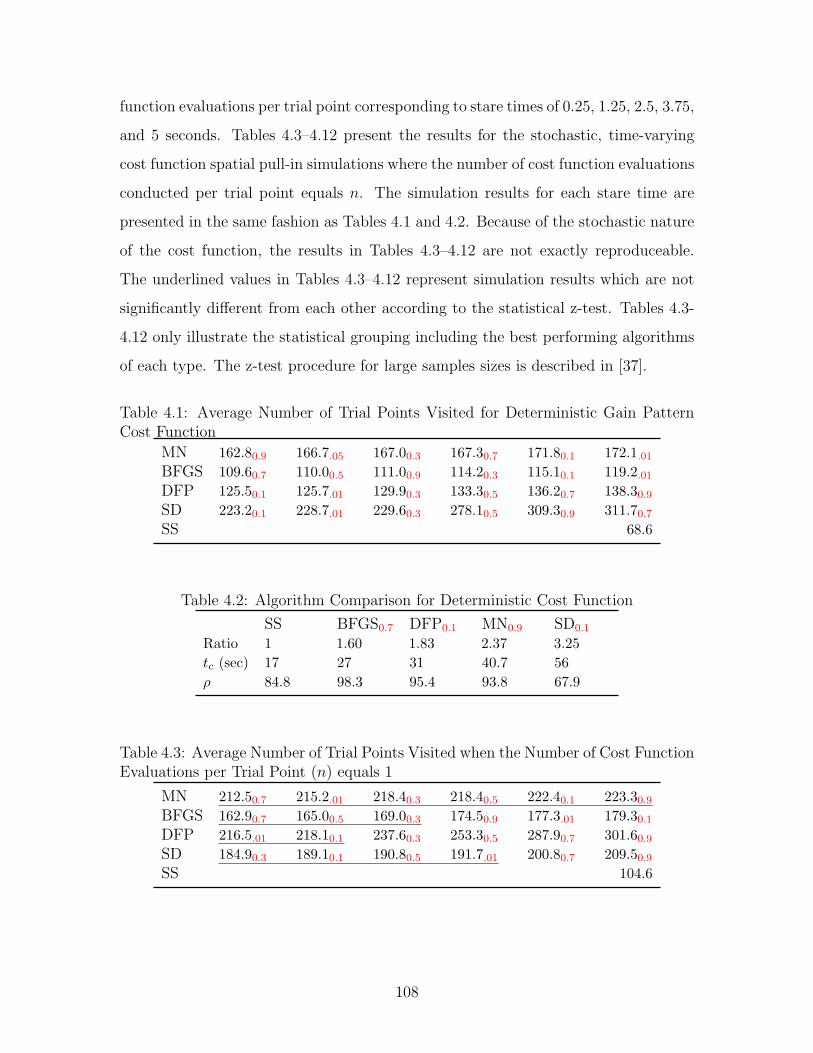
function evaluations per trial point corresponding to stare times of 0.25, 1.25, 2.5, 3.75,
and 5 seconds. Tables 4.3–4.12 present the results for the stochastic, time-varying
cost function spatial pull-in simulations where the number of cost function evaluations
conducted per trial point equals n. The simulation results for each stare time are
presented in the same fashion as Tables 4.1 and 4.2. Because of the stochastic nature
of the cost function, the results in Tables 4.3–4.12 are not exactly reproduceable.
The underlined values in Tables 4.3–4.12 represent simulation results which are not
significantly different from each other according to the statistical z-test. Tables 4.3-
4.12 only illustrate the statistical grouping including the best performing algorithms
of each type. The z-test procedure for large samples sizes is described in [37].
Table 4.1: Average Number of Trial Points Visited for Deterministic Gain PatternCost Function
MN 162.80.9 166.7.05 167.00.3 167.30.7 171.80.1 172.1.01
BFGS 109.60.7 110.00.5 111.00.9 114.20.3 115.10.1 119.2.01
DFP 125.50.1 125.7.01 129.90.3 133.30.5 136.20.7 138.30.9
SD 223.20.1 228.7.01 229.60.3 278.10.5 309.30.9 311.70.7
SS 68.6
Table 4.2: Algorithm Comparison for Deterministic Cost Function
SS BFGS0.7 DFP0.1 MN0.9 SD0.1
Ratio 1 1.60 1.83 2.37 3.25tc (sec) 17 27 31 40.7 56ρ 84.8 98.3 95.4 93.8 67.9
Table 4.3: Average Number of Trial Points Visited when the Number of Cost FunctionEvaluations per Trial Point (n) equals 1
MN 212.50.7 215.2.01 218.40.3 218.40.5 222.40.1 223.30.9
BFGS 162.90.7 165.00.5 169.00.3 174.50.9 177.3.01 179.30.1
DFP 216.5.01 218.10.1 237.60.3 253.30.5 287.90.7 301.60.9
SD 184.90.3 189.10.1 190.80.5 191.7.01 200.80.7 209.50.9
SS 104.6
108
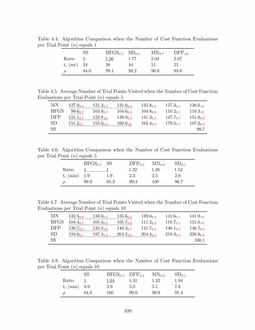
Table 4.4: Algorithm Comparison when the Number of Cost Function Evaluationsper Trial Point (n) equals 1
SS BFGS0.7 SD0.3 MN0.7 DFP.01
Ratio 1 1.56 1.77 2.03 2.07tc (sec) 24 38 44 51 51ρ 84.0 99.1 98.2 96.0 93.0
Table 4.5: Average Number of Trial Points Visited when the Number of Cost FunctionEvaluations per Trial Point (n) equals 5
MN 127.90.9 131.20.7 131.60.3 135.80.5 137.30.1 138.6.01
BFGS 99.60.7 103.90.5 104.60.3 104.80.9 110.20.1 110.3.01
DFP 121.10.1 122.8.01 139.90.3 141.20.5 147.70.7 151.80.9
SD 151.20.1 155.00.3 160.0.01 163.40.5 179.50.7 187.20.9
SS 99.7
Table 4.6: Algorithm Comparison when the Number of Cost Function Evaluationsper Trial Point (n) equals 5
BFGS0.7 SS DFP0.1 MN0.9 SD0.1
Ratio 1 1 1.22 1.28 1.52tc (min) 1.9 1.9 2.3 2.5 2.9ρ 99.9 85.3 99.3 100 96.7
Table 4.7: Average Number of Trial Points Visited when the Number of Cost FunctionEvaluations per Trial Point (n) equals 10
MN 132.50.9 133.00.7 135.60.5 139.00.3 141.60.1 141.9.01
BFGS 104.40.7 105.40.5 105.70.9 111.20.3 118.70.1 121.6.01
DFP 130.70.1 135.0.01 140.30.7 141.70.5 146.10.3 146.70.9
SD 194.00.1 197.40.3 204.3.01 204.40.5 219.30.3 226.80.9
SS 100.1
Table 4.8: Algorithm Comparison when the Number of Cost Function Evaluationsper Trial Point (n) equals 10
SS BFGS0.7 DFP0.1 MN0.9 SD0.1
Ratio 1 1.04 1.31 1.32 1.94tc (min) 3.9 3.9 5.0 5.1 7.6ρ 84.8 100 99.0 99.9 91.4
109
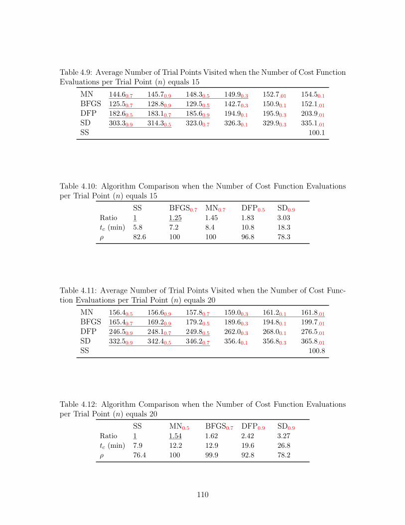
Table 4.9: Average Number of Trial Points Visited when the Number of Cost FunctionEvaluations per Trial Point (n) equals 15
MN 144.60.7 145.70.9 148.30.5 149.90.3 152.7.01 154.50.1
BFGS 125.50.7 128.80.9 129.50.5 142.70.3 150.90.1 152.1.01
DFP 182.60.5 183.10.7 185.60.9 194.90.1 195.90.3 203.9.01
SD 303.30.9 314.30.5 323.00.7 326.30.1 329.90.3 335.1.01
SS 100.1
Table 4.10: Algorithm Comparison when the Number of Cost Function Evaluationsper Trial Point (n) equals 15
SS BFGS0.7 MN0.7 DFP0.5 SD0.9
Ratio 1 1.25 1.45 1.83 3.03tc (min) 5.8 7.2 8.4 10.8 18.3ρ 82.6 100 100 96.8 78.3
Table 4.11: Average Number of Trial Points Visited when the Number of Cost Func-tion Evaluations per Trial Point (n) equals 20
MN 156.40.5 156.60.9 157.80.7 159.00.3 161.20.1 161.8.01
BFGS 165.40.7 169.20.9 179.20.5 189.60.3 194.80.1 199.7.01
DFP 246.50.9 248.10.7 249.80.5 262.00.3 268.00.1 276.5.01
SD 332.50.9 342.40.5 346.20.7 356.40.1 356.80.3 365.8.01
SS 100.8
Table 4.12: Algorithm Comparison when the Number of Cost Function Evaluationsper Trial Point (n) equals 20
SS MN0.5 BFGS0.7 DFP0.9 SD0.9
Ratio 1 1.54 1.62 2.42 3.27tc (min) 7.9 12.2 12.9 19.6 26.8ρ 76.4 100 99.9 92.8 78.2
110
4.5.1 Observations
Based on the spatial pull-in simulation results presented in Tables 4.3–4.12 one con-
cludes that the SS and BFGS step-tracking algorithms consistently outperform the
other algorithms. As alluded to in Section 4.3.2, the SS algorithm has convergence
limitations and displays a maximum convergence percentage of only 85% for the n=5
scenario (Table 4.6). Most of the nonlinear optimization step-tracking algorithms
display convergence percentages upwards of 90% under most circumstances. The
BFGS algorithm consistently displays high convergence percentages of 98% or better.
Although the BFGS algorithm typically requires a higher number of trial points to
reach convergence than does the SS algorithm, the difference in convergence times
between the two step-tracking methods is negligible for shorter stare times (n < 15).
The spatial pull-in simulation results shed light on what the optimal stare time
should be for a step-tracking algorithm implemented on an airborne SATCOM ter-
minal. Even though Equation (4.33) determined that 16 cost function measurements
per trial point are necessary to reduce the pointing error confidence interval to 0.02,
such a large value of n is, in fact, undesirable. Figure 4-10 shows a scatter plot of
the convergence times versus n for each of the step-tracking algorithms tested. From
Figure 4-10, one sees that measuring the cost function only once at each trial point
visited by the step-tracking algorithm produces convergence times much shorter than
measuring the cost function 5, 10, 15, or 20 times per trial point. Tables 4.3 and
4.5 indicate that the step-tracking algorithms visit a greater number of trial points
for a stare time of 0.25 seconds than for a stare time of 1.25 seconds; however, the
time spent at each trial point when the stare time is 1.25 seconds increases the total
convergence time substantially.
The results of the spatial pull-in simulations suggest the optimal linear search pa-
rameter that should be used in each of the different optimization algorithms for the
selected stare times. The optimal linear search parameters for the algorithms in the
deterministic simulations are the same, within the statistical significance groupings,
as the optimal linear search parameters in the stochastic simulations for the n=1, 5,
111
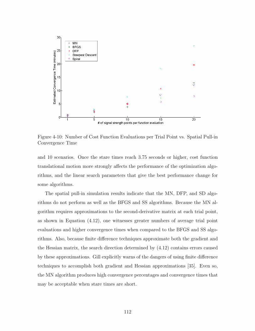
Figure 4-10: Number of Cost Function Evaluations per Trial Point vs. Spatial Pull-inConvergence Time
and 10 scenarios. Once the stare times reach 3.75 seconds or higher, cost function
translational motion more strongly affects the performance of the optimization algo-
rithms, and the linear search parameters that give the best performance change for
some algorithms.
The spatial pull-in simulation results indicate that the MN, DFP, and SD algo-
rithms do not perform as well as the BFGS and SS algorithms. Because the MN al-
gorithm requires approximations to the second-derivative matrix at each trial point,
as shown in Equation (4.12), one witnesses greater numbers of average trial point
evaluations and higher convergence times when compared to the BFGS and SS algo-
rithms. Also, because finite difference techniques approximate both the gradient and
the Hessian matrix, the search direction determined by (4.12) contains errors caused
by these approximations. Gill explicitly warns of the dangers of using finite difference
techniques to accomplish both gradient and Hessian approximations [35]. Even so,
the MN algorithm produces high convergence percentages and convergence times that
may be acceptable when stare times are short.
112
The DFP algorithm differs from the BFGS algorithm only by the update matrix
formula presented in Equation (4.23). The literature suggests that BFGS algorithms
may out-perform DFP methods by as much as an order of magnitude in some instances
[34]. For the spatial pull-in simulations, BFGS step-tracking algorithms consistently
out-perform algorithms incorporating DFP optimization methods; therefore, BFGS
methods should be favored for use in step-tracking applications.
Because of the radial nature of the gain pattern cost function, Steepest Descent
methods produce search directions which provide the shortest paths to minima in the
cost function when the cost function is deterministic and the errors caused by finite
differencing are ignored. SD methods rely heavily on accurate linear searches which
are accomplished more easily when drastic changes to the initial step length, α0, are
not required. Equation (4.25) shows that the initial step length for the SD algorithm
equals the magnitude of the gradient vector, which could be quite large. Even if
the magnitude of the initial step length is restricted to a 1 region of confidence, as
described in Section 4.4.4, a 1 initial step size could be too large when the trial
point lies in the vicinity of a minima. In these instances, the linear search procedure
must work hard both to bracket a minimum and to find a step length that meets
the criterion in Equation (4.31). Newton methods typically generate initial step sizes
that already meet the linear search requirement in Equation (4.31); therefore, Newton
methods outperform the SD method in nearly all the spatial pull-in simulations.
4.6 Spatial Pull-in Robustness Tests
The two best-performing algorithms in Section 4.5, the SS algorithm and the BFGS
algorithm with η = 0.7, were subjected to spatial pull-in tests under harsher con-
ditions in order to test the robustness of each of the methods. The spatial pull-in
robustness simulations incorporate greater open-loop pointing errors by increasing
the variances on the inertial angular components of pointing error. The robust-
ness simulations also exhibit faster translational movement (vpat) of the cost function
to simulate more drastic time-varying sources of open-loop pointing error or more
113
pronounced satellite motion. Both algorithms in the spatial pull-in robustness sim-
ulations conduct spatial pull-in from the same 1024 starting locations displayed in
Figure 4-8.
During the robustness simulations, both the SS and BFGS algorithms were left in
the same configurations used in the spatial pull-in tests conducted in Section 4.5. The
spatial pull-in tests for increased pointing error variances and cost function velocities
incorporated stare times of 0.25 and 1.25 seconds. Tables 4.13 and 4.14 present the
results of the robustness simulations. The ratio value is the ratio of the average
number of trial points visited for the particular velocity-variance combination listed
in the given column compared to the number of trial points visited for the velocity-
variance combination in the first column. The results listed in the first column of
Tables 4.13 and 4.14 are the same as the results from the corresponding tests in
Section 4.5. Tables 4.13 and 4.14 calculate convergence times (tc) and percentages
(ρ) according to Equations (4.34)–(4.35).
4.6.1 Observations
As expected, the performance of both algorithms degrades as the pointing error vari-
ances and pattern velocities are increased. Tables 4.13–4.14 show performance drops
in terms of average number of trial points visited, convergence times, and convergence
percentages. The underlined values in Tables 4.13–4.14 represent simulation results
that are not statistically different from each other according to the z-test. For the
n=1 scenario, the BFGS step-tracking algorithm feels the effects of the worsening
pointing error and pattern velocity conditions much more so than the SS algorithm.
The convergence percentage of the BFGS algorithm drops significantly for the last two
velocity-variance combinations and average convergence times are nearly tripled. The
SS algorithm demonstrates only slight drops in convergence percentages and slight in-
creases in convergence times as conditions worsen for the n=1 case. For the n=5 case,
the BFGS algorithm maintains convergence percentages greater than 95%. Table 4.14
shows that average convergence times are doubled for the BFGS approach under the
harshest velocity-variance conditions of the test when n=5. The SS algorithm ex-
114

Table 4.13: Spatial Pull-in Robustness Simulation (Number of Cost Function Evalu-ations per Trial Point (n) equals 1)
velocity/variance5e-4/4e-4
1e-3/4e-4
5e-4/8e-4
1e-3/8e-4
2e-3/8e-4
1e-3/1.6e-3
2e-3/1.6e-3
BFGSRatio 1 1.01 1.68 1.64 1.64 2.44 2.42tc (sec) 38 39 64 64 66 96 96ρ 99.1 99.5 92.6 92.5 90.4 73.2 70.9
SSRatio 1 1 1.07 1.07 1.08 1.20 1.22tc (sec) 24 24 26 26 26 30 30ρ 84.0 85.4 84.7 85.3 85.6 83.4 83.3
Table 4.14: Spatial Pull-in Robustness Simulation (Number of Cost Function Evalu-ations per Trial Point (n) equals 5)
velocity/variance5e-4/4e-4
1e-3/4e-4
5e-4/8e-4
1e-3/8e-4
2e-3/8e-4
1e-3/1.6e-3
2e-3/1.6e-3
BFGSRatio 1 1.09 1.11 1.21 1.61 1.68 2.15tc (min) 1.9 2.1 2.1 2.3 3.1 3.3 4.2ρ 99.9 100 99.9 99.8 98.8 99.6 95.1
SSRatio 1 1.01 1.03 1.06 1.06 1.14 1.13tc (min) 1.9 2.0 2.0 2.0 2.1 2.2 2.2ρ 85.3 84.4 84.6 84.4 65.6 51.0 83.1
115
hibits significant drops in convergence percentages for the harsher velocity-variance
combinations in the n=5 scenario, but the average convergence time is only slightly
increased.
The engineer must decide how to structure the step-tracking algorithm to provide
adequate spatial pull-in performance when open-loop pointing errors impose harsher
conditions on the cost function. The SS algorithm may be used with a negligible stare
time (n=1) to provide quick convergence times while achieving convergence rates of
approximately 85% at best. If higher convergence percentages for spatial pull-in are
desired, the engineer may opt to use the BFGS algorithm while incorporating a brief
stare time, such as 1.25 seconds for the n=5 case. The added stare time produces
longer convergence times but may be worth the trade-off for added convergence per-
centages.
4.7 A Look at Tracking
To demonstrate how step-tracking algorithms may be applied to accomplishing closed-
loop tracking of a target satellite, the BFGS algorithm with a linear search parameter
of 0.7 undergoes a series of tracking simulations. Separate tracking simulations were
conducted for each of the pointing error variance and cost function velocity pairs used
in Section 4.6. In a tracking configuration, the BFGS algorithm removes the terminal
conditions imposed during spatial pull-in. The algorithm tracks the target satellite
by continuously minimizing the gain pattern cost function until 500 trial points are
evaluated in each simulation. Tracking performance of the BFGS algorithm was ex-
amined for both the n=1 and n=5 cases. According to Equation (4.34), for the n=1
scenario, tracking was accomplished for approximately 125 seconds per simulation,
and for the n=5 case, tracking was accomplished for approximately 625 seconds per
simulation. Each of the tracking simulations were conducted beginning from 1024
starting locations within a 0.1 radius from boresight (Figure 4-11). The close prox-
imity of the initial starting points in the tracking simulations to boresight simulates
the result of an accurate spatial pull-in procedure. During the tracking simulations,
116
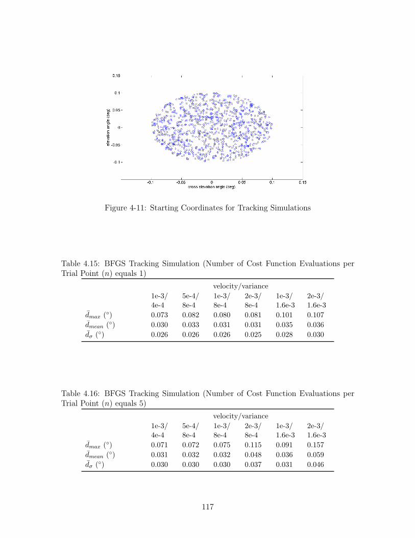
Figure 4-11: Starting Coordinates for Tracking Simulations
Table 4.15: BFGS Tracking Simulation (Number of Cost Function Evaluations perTrial Point (n) equals 1)
velocity/variance1e-3/4e-4
5e-4/8e-4
1e-3/8e-4
2e-3/8e-4
1e-3/1.6e-3
2e-3/1.6e-3
dmax () 0.073 0.082 0.080 0.081 0.101 0.107dmean () 0.030 0.033 0.031 0.031 0.035 0.036dσ () 0.026 0.026 0.026 0.025 0.028 0.030
Table 4.16: BFGS Tracking Simulation (Number of Cost Function Evaluations perTrial Point (n) equals 5)
velocity/variance1e-3/4e-4
5e-4/8e-4
1e-3/8e-4
2e-3/8e-4
1e-3/1.6e-3
2e-3/1.6e-3
dmax () 0.071 0.072 0.075 0.115 0.091 0.157dmean () 0.031 0.032 0.032 0.048 0.036 0.059dσ () 0.030 0.030 0.030 0.037 0.031 0.046
117
the maximum distance from boresight (dmax), mean distance from boresight (dmean),
and standard deviation of the distance from boresight (dσ) were recorded for each
starting location in Figure 4-11. Table 4.15 summarizes the mean of these three met-
rics over all 1024 initial starting points for each pointing error variance and pattern
velocity combination for the n=1 case. Table 4.16 displays the results for the n=5
case. The bar above the metrics in Tables 4.15–4.16 indicates an average value.
4.7.1 Observations
Tables 4.15 and 4.16 demonstrate satisfactory tracking performance from the BFGS
step-tracking algorithm. The average maximum deviations from boresight, dmax,
never exceed the 0.25 requirement outlined in Section 2.3, and the average mean de-
viations from boresight, dmean, are lower still. Even when the pointing error variances
and pattern velocities are increased to values higher than those assumed for the op-
erating environment of the nominal APS, the BFGS algorithm remains comfortably
within the 0.25 requirement for closed-loop operation. Tracking for the n=1 case
slightly outperforms the n=5 case for higher velocity-variance combinations.
4.8 Simulation Processing Times
Each of the individual spatial pull-in, and tracking simulations consumes a substan-
tial amount of processing time because each simulation involves either spatial pull-in
or tracking from 1024 starting locations. Figure 4-8 shows the starting locations for
the spatial pull-in simulations, and Figure 4-11 depicts the initial trial points for
the tracking simulations. To carry out the spatial pull-in and tracking simulations
presented in this chapter, the step-tracking algorithms found in Appendix C were
modified to run on a parallel processing network located at MIT Lincoln Laboratory
known as the LLGrid. In each simulation, each of the 1024 starting locations gets
assigned to one of 64 networked computers on the LLGrid; thus, a single computer
becomes responsible for conducting either spatial pull-in or tracking from only 16
initial test points per simulation rather than all 1024. To compare the benefits of
118
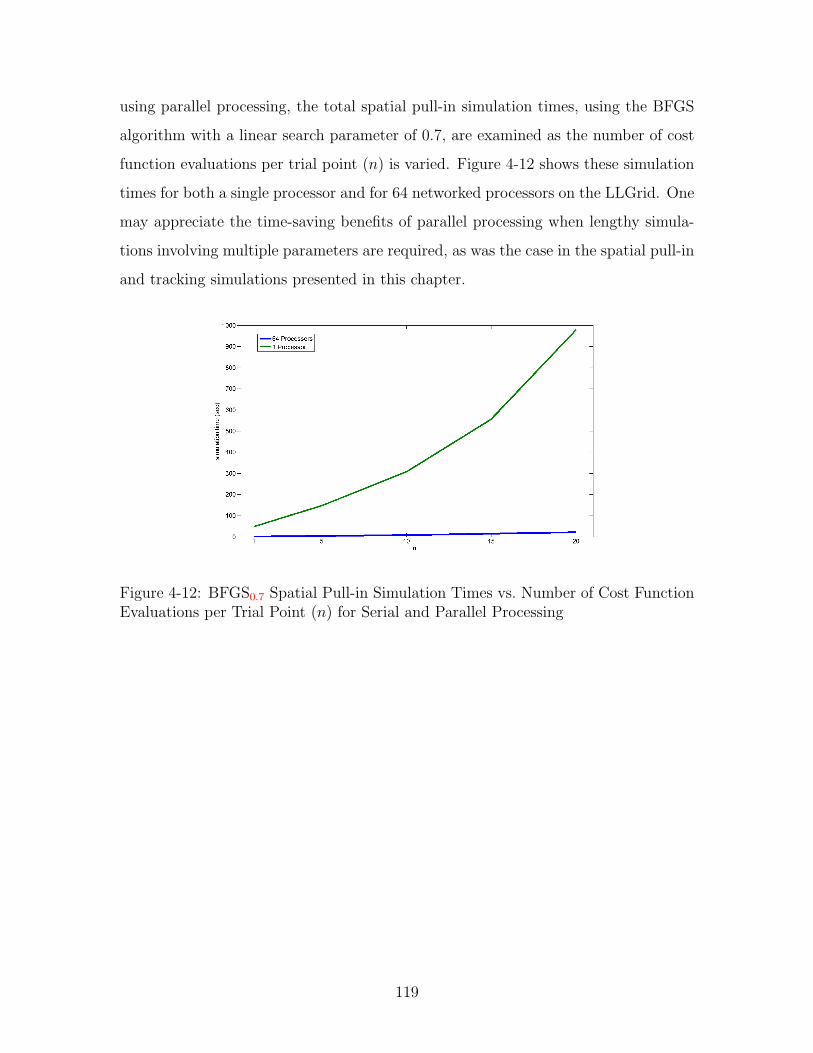
using parallel processing, the total spatial pull-in simulation times, using the BFGS
algorithm with a linear search parameter of 0.7, are examined as the number of cost
function evaluations per trial point (n) is varied. Figure 4-12 shows these simulation
times for both a single processor and for 64 networked processors on the LLGrid. One
may appreciate the time-saving benefits of parallel processing when lengthy simula-
tions involving multiple parameters are required, as was the case in the spatial pull-in
and tracking simulations presented in this chapter.
Figure 4-12: BFGS0.7 Spatial Pull-in Simulation Times vs. Number of Cost FunctionEvaluations per Trial Point (n) for Serial and Parallel Processing
119

120
Chapter 5
Conclusions
5.1 Open-loop Controller Simulation Results Sum-
mary
This thesis developed a hybrid open/closed-loop antenna pointing strategy for the
nominal APS defined in Section 2.3. To accomplish open-loop pointing, a pedestal
feedback controller was designed using state-space and optimal control techniques.
The feedback controller mitigates the effects of base motion disturbances caused by
vehicle motion and tracks reference commands issued by the closed-loop portion of the
hybrid pointing scheme. The performance of the controller on both a linearized plant
model and a more detailed nonlinear plant model was examined through simulation
in Sections 3.2.5–3.2.6.
The controller was found to point the antenna of the nominal APS to a loca-
tion in inertial space within the 0.1 requirement for open-loop pointing error before
considering the effects of potential sources of error. Because the simulation results
indicate that the pedestal feedback controller developed in Chapter 3 is capable of
meeting the design requirement for open-loop pointing, the open-loop portion of the
hybrid open/closed-loop strategy is deemed satisfactory. When sources of open-loop
pointing error are introduced to the antenna pointing problem in mobile SATCOM
applications, some form of closed-loop pointing is desired.
121
5.2 Closed-loop Step-tracking Simulation Results
Summary
Step-tracking methods were investigated for the nominal APS because they require no
additional hardware components and effectively offer the simplest method of closed-
loop antenna pointing. Four step-tracking algorithms were developed using methods
of nonlinear cost function optimization along with a fifth algorithm developed using
a spiral search function comparison technique. The closed-loop spatial pull-in per-
formance of the five step-tracking algorithms was tested through simulation. The
first set of spatial pull-in simulations assumed a particular operating environment for
the nominal APS in an airborne SATCOM application. This environment includes a
stochastic cost function, caused by open-loop inertial pointing errors, and a cost func-
tion that translates in inertial space due to satellite motion and an assumed amount
of time-varying open-loop pointing error (See Section 4.5).
The results of the spatial pull-in simulations, presented in Tables 4.1–4.12, illus-
trate that the BFGS and SS algorithms outperform the remainder of the step-tracking
algorithms. To meet the closed-loop pointing requirement outlined in Section 2.3, the
step-tracking algorithms must converge to within 0.25 of boresight in the spatial
pull-in stage. The BFGS algorithm displays very high percentages of convergence to
within the 0.25 requirement (upwards of 98%) and demonstrates average convergence
times on the same order as the SS algorithm for shorter stare times (n < 15). On
average, the SS algorithm converges to within 0.25 of boresight more quickly than
the BFGS algorithm but exhibits convergence percentages of only 85% or worse. The
first set of spatial pull-in tests also demonstrate that stare times should typically be
made as short as possible to achieve the quickest convergence times (Figure 4-10).
In these tests, the average spatial pull-in convergence times for negligible stare times
(n = 1) are less than a minute (Table 4.4).
The performance of the BFGS and SS algorithms was tested through simulation for
harsher operating environments where greater open-loop pointing errors and larger
effects of time-varying sources of open-loop pointing error were considered. The
122
results of the step-tracking algorithm robustness tests, presented in Tables 4.13 and
4.14, demonstrate that the SS algorithm continues to perform better for negligible
stare times (n = 1); whereas, the BFGS algorithm performs better when a short
stare time is incorporated, as in the n = 5 case. The SS algorithm in the n = 1
configuration shows average convergence times of 30 seconds or faster but continues
to have convergence percentages of only 85% at best. The BFGS algorithm in the
n = 5 configuration maintains convergence percentages of 95% or better but average
convergence times are extended to around 4 minutes for the harshest of the velocity-
variance combinations. When operating environments are worse than those assumed
for the nominal APS, the engineer may select a SS step-tracking method, with quick
convergence times and lower convergence percentages, or sacrifice convergence time for
higher reliability with the BFGS approach. For many mobile SATCOM applications,
wait times for accomplishing spatial pull-in of up to 5 minutes may be acceptable and
worth the trade-off for the higher convergence percentages provided by the BFGS
algorithm.
Because the SS function comparison algorithm cannot be used for tracking without
major modifications to the algorithm structure, only the BFGS algorithm was im-
plemented in closed-loop tracking simulations. To gauge the robustness of the BFGS
algorithm in a tracking configuration, the tracking simulations were conducted for the
same velocity-variance combinations used in the spatial pull-in robustness tests. The
tracking simulations incorporated stare times of 0.25 and 1.25 seconds. The results
of the tracking simulations presented in Tables 4.15 and 4.16 support the conclusion
that a BFGS step-tracking algorithm could be used to maintain closed-loop inertial
tracking to within the 0.25 requirement even in harsher operating environments than
assumed for the nominal APS. The results of the tracking simulations also indicate
that stare times should be kept as short as possible to achieve the best tracking
performance.
123

5.3 Overall Contributions
Major contributions made by the research presented in this thesis are listed below:
1. Using optimal and state-space control techniques, this thesis developed an open-
loop pedestal controller for a nominal, two-axis, azimuth-elevation APS that
mitigates the effects of aircraft motion and tracks input reference commands.
The techniques used to develop the pedestal controller for the nominal APS may
be applied to other mobile SATCOM projects where two-axis, azimuth-elevation
pedestals are employed to accomplish antenna pointing.
2. A Simulink simulation was developed to simulate the pointing performance of
the open-loop pedestal controller on the nominal APS. The simulation may be
easily modified and used to determine the open-loop pointing performance of
similar APSs used on other SATCOM projects.
3. Closed-loop step tracking algorithms were developed and shown to offer vi-
able solutions for accomplishing closed-loop antenna pointing on an airborne
SATCOM terminal. Both the BFGS and SS algorithms offer acceptable meth-
ods for accomplishing spatial pull-in even under conditions worse than those
assumed for the nominal APS. The BFGS method provides more reliable con-
vergence guarantees at the expense of slightly longer convergence times while
the SS algorithm performs in the opposite manner.
4. The BFGS step-tracking algorithm was shown to effectively accomplish closed-
loop target satellite tracking. In a tracking configuration, the BFGS algorithm
maintained inertial pointing to within the 0.25 of boresight requirement even
when the operating conditions were harsher than those assumed for the nominal
APS.
5. Because simulation results indicate that both the open-loop feedback controller
and select closed-loop step-tracking methods meet the requirements for the nom-
inal APS, the hybrid open/closed-loop approach to antenna pointing is consid-
124
ered feasible for an airborne SATCOM application. Both the open-loop con-
troller development techniques, and the closed-loop step-tracking algorithms,
may be applied to other SATCOM applications, either mobile or stationary. Be-
cause this thesis has shown a hybrid open/closed-loop antenna pointing strategy
to be feasible, accurate antenna pointing may be accomplished with a simple,
cost-effective APS without the need for more complex systems involving addi-
tional closed-loop tracking hardware.
5.4 Suggestions for Future Work
The Simulink model developed in Section 3.2.6 provides insight as to how the nominal
APS, while operating in an open-loop fashion, may actually perform while operating in
an airborne environment. As more complex pedestal dynamics models are developed,
the new effects may easily be added to the simulation and their impact on the overall
pointing error may be readily observed. In particular, models simulating the effects
of the open-loop sources of error, identified in Section 2.2.1, may be added to the
existing simulation. The MATLAB scripts for the step-tracking algorithms, located
in Appendix C, may be converted into Simulink models and the entire open/closed-
loop system could be simulated together in one location. The combined simulation
could provide greater insights to using hybrid pointing strategies on mobile SATCOM
terminals.
The open-loop controller developed in Chapter 3 yielded a system with a band-
width of only approximately 2.5 Hz because the harshest disturbance inputs occurred
at much lower frequencies (Figures 3-3 and 3-8). If the closed-loop pedestal con-
troller bandwidth could be increased, the step time between trial points could be
reduced. Consequently, the convergence times for the closed-loop step-tracking algo-
rithms could be lowered as the time spent traveling between trial points would be
reduced.
Both the SS and BFGS algorithms showed promising results for step-tracking
approaches to accomplishing spatial pull-in. A combined SS/BFGS algorithm could
125
be developed that achieves shorter average convergence times than a standard BFGS
approach, but higher convergence percentages than a stand-alone SS algorithm. The
hybrid SS/BFGS step-tracking approach could begin the spatial pull-in process with
an SS method and then switch to a BFGS method once the SS algorithm terminates.
If boresight is not located when the SS algorithm terminates, the BFGS algorithm
could accomplish the remainder of the spatial pull-in task. Convergence times would
be reduced by allowing the SS algorithm to accomplish as much of the spatial pull-in
task as possible before engaging the slower BFGS algorithm.
This thesis has shown through simulation the feasibility of using hybrid open/closed-
loop pointing strategies on mobile SATCOM terminals. The suggested next step in
implementing hybrid pointing strategies on actual terminal systems involves a series
of hardware tests. First, the pointing strategy should be applied to a terminal system
operating on the ground with no base motion disturbances. Secondly, pointing tests
may be conducted with the pedestal system operating on a motion simulator table
to mimic different mobile environments. Finally, the pointing strategy may be tested
with a vehicle-mounted APS. The tests occur in increasing order of complexity so
that issues with using a hybrid pointing strategy may be identified at the lowest level
and testing costs may be kept to a minimum.
126
Appendix A
Satellite Look Angle Calculations
Overview
This appendix presents two ways of calculating the desired local azimuth and elevation
look angles, azd and eld, and their rates, azd and eld, for airborne inertial pointing
applications using two-axis positioners. The first method involves finding position and
relative velocity vectors from a mobile terminal to a target satellite based on kinematic
relationships derived from the satellite’s orbital element set and the terminal’s GPS
location and inertial states. The second method calculates local look angles and their
rates if the desired inertial look angles are known in addition to the terminal’s inertial
information.
In this thesis, the “inertial” qualifier refers to the topocentric North, East, Down
(NED) reference frame. The NED frame rotates with the Earth and, therefore, is not
strictly an inertial reference frame. However, engineers still regard the NED coordi-
nate system as an inertial reference frame in many circumstances because rotations
of objects in this frame are generally much faster than the rotation of the coordinate
system itself [24].
The following generic formulas are used throughout this appendix to calculate
look angles and look angle rates:
127
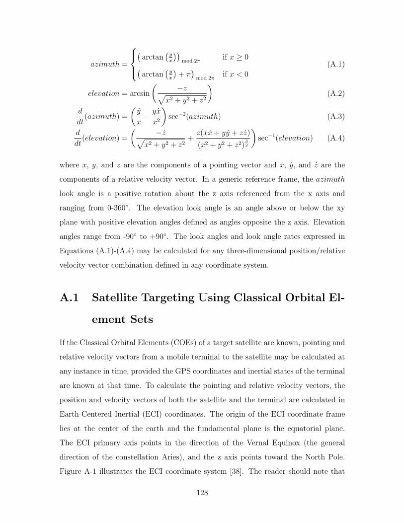
azimuth =
(
arctan(yx
))mod 2π
if x ≥ 0(arctan
(yx
)+ π)
mod 2πif x < 0
(A.1)
elevation = arcsin
(−z√
x2 + y2 + z2
)(A.2)
d
dt(azimuth) =
(y
x− yx
x2
)sec−2(azimuth) (A.3)
d
dt(elevation) =
(−z√
x2 + y2 + z2+z(xx+ yy + zz)
(x2 + y2 + z2)32
)sec−1(elevation) (A.4)
where x, y, and z are the components of a pointing vector and x, y, and z are the
components of a relative velocity vector. In a generic reference frame, the azimuth
look angle is a positive rotation about the z axis referenced from the x axis and
ranging from 0-360. The elevation look angle is an angle above or below the xy
plane with positive elevation angles defined as angles opposite the z axis. Elevation
angles range from -90 to +90. The look angles and look angle rates expressed in
Equations (A.1)-(A.4) may be calculated for any three-dimensional position/relative
velocity vector combination defined in any coordinate system.
A.1 Satellite Targeting Using Classical Orbital El-
ement Sets
If the Classical Orbital Elements (COEs) of a target satellite are known, pointing and
relative velocity vectors from a mobile terminal to the satellite may be calculated at
any instance in time, provided the GPS coordinates and inertial states of the terminal
are known at that time. To calculate the pointing and relative velocity vectors, the
position and velocity vectors of both the satellite and the terminal are calculated in
Earth-Centered Inertial (ECI) coordinates. The origin of the ECI coordinate frame
lies at the center of the earth and the fundamental plane is the equatorial plane.
The ECI primary axis points in the direction of the Vernal Equinox (the general
direction of the constellation Aries), and the z axis points toward the North Pole.
Figure A-1 illustrates the ECI coordinate system [38]. The reader should note that
128
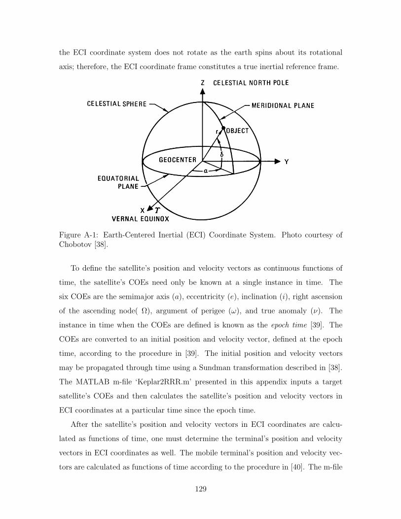
the ECI coordinate system does not rotate as the earth spins about its rotational
axis; therefore, the ECI coordinate frame constitutes a true inertial reference frame.
Figure A-1: Earth-Centered Inertial (ECI) Coordinate System. Photo courtesy ofChobotov [38].
To define the satellite’s position and velocity vectors as continuous functions of
time, the satellite’s COEs need only be known at a single instance in time. The
six COEs are the semimajor axis (a), eccentricity (e), inclination (i), right ascension
of the ascending node( Ω), argument of perigee (ω), and true anomaly (ν). The
instance in time when the COEs are defined is known as the epoch time [39]. The
COEs are converted to an initial position and velocity vector, defined at the epoch
time, according to the procedure in [39]. The initial position and velocity vectors
may be propagated through time using a Sundman transformation described in [38].
The MATLAB m-file ‘Keplar2RRR.m’ presented in this appendix inputs a target
satellite’s COEs and then calculates the satellite’s position and velocity vectors in
ECI coordinates at a particular time since the epoch time.
After the satellite’s position and velocity vectors in ECI coordinates are calcu-
lated as functions of time, one must determine the terminal’s position and velocity
vectors in ECI coordinates as well. The mobile terminal’s position and velocity vec-
tors are calculated as functions of time according to the procedure in [40]. The m-file
129
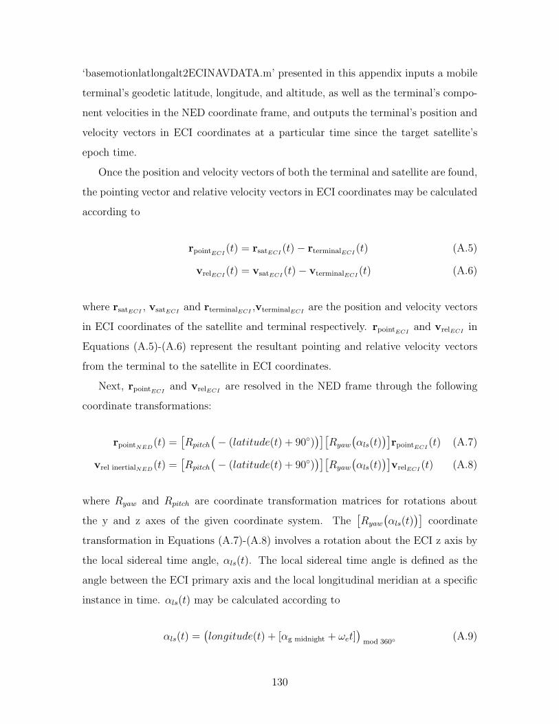
‘basemotionlatlongalt2ECINAVDATA.m’ presented in this appendix inputs a mobile
terminal’s geodetic latitude, longitude, and altitude, as well as the terminal’s compo-
nent velocities in the NED coordinate frame, and outputs the terminal’s position and
velocity vectors in ECI coordinates at a particular time since the target satellite’s
epoch time.
Once the position and velocity vectors of both the terminal and satellite are found,
the pointing vector and relative velocity vectors in ECI coordinates may be calculated
according to
rpointECI (t) = rsatECI (t)− rterminalECI (t) (A.5)
vrelECI (t) = vsatECI (t)− vterminalECI (t) (A.6)
where rsatECI , vsatECI and rterminalECI ,vterminalECI are the position and velocity vectors
in ECI coordinates of the satellite and terminal respectively. rpointECI and vrelECI in
Equations (A.5)-(A.6) represent the resultant pointing and relative velocity vectors
from the terminal to the satellite in ECI coordinates.
Next, rpointECI and vrelECI are resolved in the NED frame through the following
coordinate transformations:
rpointNED(t) =[Rpitch
(− (latitude(t) + 90)
)][Ryaw
(αls(t)
)]rpointECI (t) (A.7)
vrel inertialNED(t) =[Rpitch
(− (latitude(t) + 90)
)][Ryaw
(αls(t)
)]vrelECI (t) (A.8)
where Ryaw and Rpitch are coordinate transformation matrices for rotations about
the y and z axes of the given coordinate system. The[Ryaw
(αls(t)
)]coordinate
transformation in Equations (A.7)-(A.8) involves a rotation about the ECI z axis by
the local sidereal time angle, αls(t). The local sidereal time angle is defined as the
angle between the ECI primary axis and the local longitudinal meridian at a specific
instance in time. αls(t) may be calculated according to
αls(t) =(longitude(t) + [αg midnight + ωet]
)mod 360
(A.9)
130
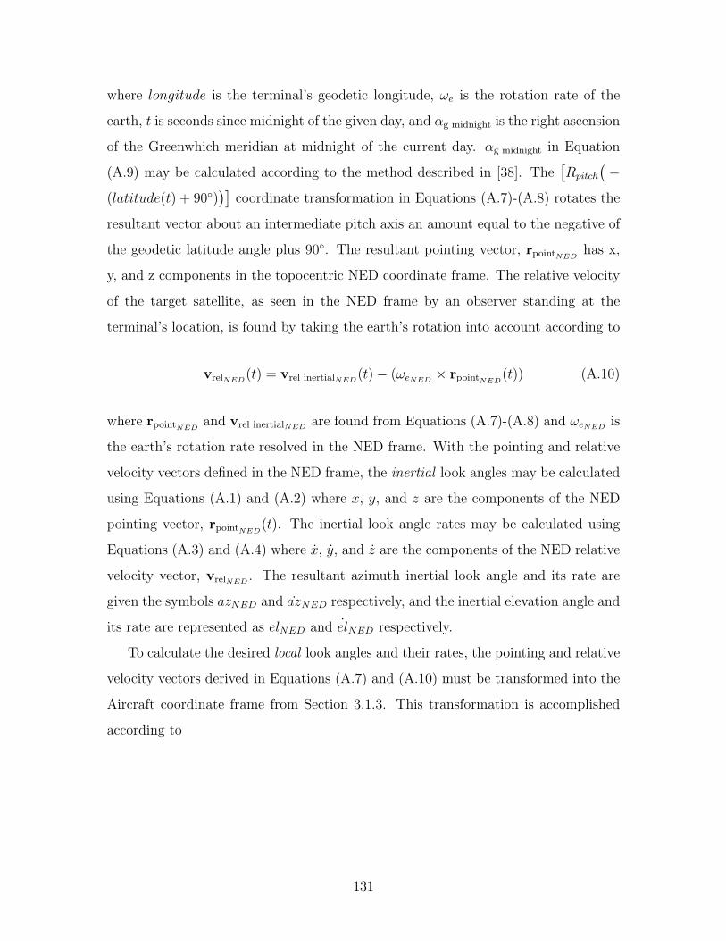
where longitude is the terminal’s geodetic longitude, ωe is the rotation rate of the
earth, t is seconds since midnight of the given day, and αg midnight is the right ascension
of the Greenwhich meridian at midnight of the current day. αg midnight in Equation
(A.9) may be calculated according to the method described in [38]. The[Rpitch
(−
(latitude(t) + 90))]
coordinate transformation in Equations (A.7)-(A.8) rotates the
resultant vector about an intermediate pitch axis an amount equal to the negative of
the geodetic latitude angle plus 90. The resultant pointing vector, rpointNED has x,
y, and z components in the topocentric NED coordinate frame. The relative velocity
of the target satellite, as seen in the NED frame by an observer standing at the
terminal’s location, is found by taking the earth’s rotation into account according to
vrelNED(t) = vrel inertialNED(t)− (ωeNED × rpointNED(t)) (A.10)
where rpointNED and vrel inertialNED are found from Equations (A.7)-(A.8) and ωeNED is
the earth’s rotation rate resolved in the NED frame. With the pointing and relative
velocity vectors defined in the NED frame, the inertial look angles may be calculated
using Equations (A.1) and (A.2) where x, y, and z are the components of the NED
pointing vector, rpointNED(t). The inertial look angle rates may be calculated using
Equations (A.3) and (A.4) where x, y, and z are the components of the NED relative
velocity vector, vrelNED . The resultant azimuth inertial look angle and its rate are
given the symbols azNED and azNED respectively, and the inertial elevation angle and
its rate are represented as elNED and elNED respectively.
To calculate the desired local look angles and their rates, the pointing and relative
velocity vectors derived in Equations (A.7) and (A.10) must be transformed into the
Aircraft coordinate frame from Section 3.1.3. This transformation is accomplished
according to
131
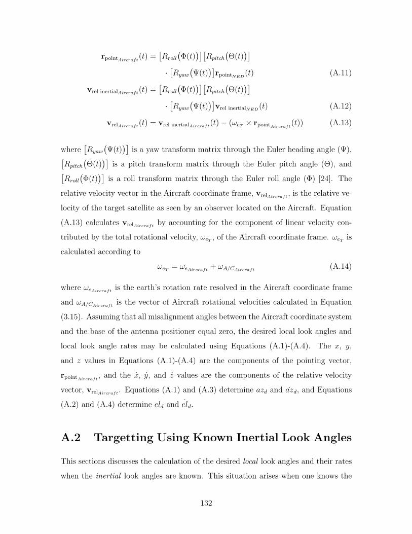
rpointAircraft(t) =[Rroll
(Φ(t)
)][Rpitch
(Θ(t)
)]·[Ryaw
(Ψ(t)
)]rpointNED(t) (A.11)
vrel inertialAircraft(t) =[Rroll
(Φ(t)
)][Rpitch
(Θ(t)
)]·[Ryaw
(Ψ(t)
)]vrel inertialNED(t) (A.12)
vrelAircraft(t) = vrel inertialAircraft(t)− (ωeT × rpointAircraft(t)) (A.13)
where[Ryaw
(Ψ(t)
)]is a yaw transform matrix through the Euler heading angle (Ψ),[
Rpitch
(Θ(t)
)]is a pitch transform matrix through the Euler pitch angle (Θ), and[
Rroll
(Φ(t)
)]is a roll transform matrix through the Euler roll angle (Φ) [24]. The
relative velocity vector in the Aircraft coordinate frame, vrelAircraft , is the relative ve-
locity of the target satellite as seen by an observer located on the Aircraft. Equation
(A.13) calculates vrelAircraft by accounting for the component of linear velocity con-
tributed by the total rotational velocity, ωeT , of the Aircraft coordinate frame. ωeT is
calculated according to
ωeT = ωeAircraft + ωA/CAircraft (A.14)
where ωeAircraft is the earth’s rotation rate resolved in the Aircraft coordinate frame
and ωA/CAircraft is the vector of Aircraft rotational velocities calculated in Equation
(3.15). Assuming that all misalignment angles between the Aircraft coordinate system
and the base of the antenna positioner equal zero, the desired local look angles and
local look angle rates may be calculated using Equations (A.1)-(A.4). The x, y,
and z values in Equations (A.1)-(A.4) are the components of the pointing vector,
rpointAircraft , and the x, y, and z values are the components of the relative velocity
vector, vrelAircraft . Equations (A.1) and (A.3) determine azd and azd, and Equations
(A.2) and (A.4) determine eld and eld.
A.2 Targetting Using Known Inertial Look Angles
This sections discusses the calculation of the desired local look angles and their rates
when the inertial look angles are known. This situation arises when one knows the
132
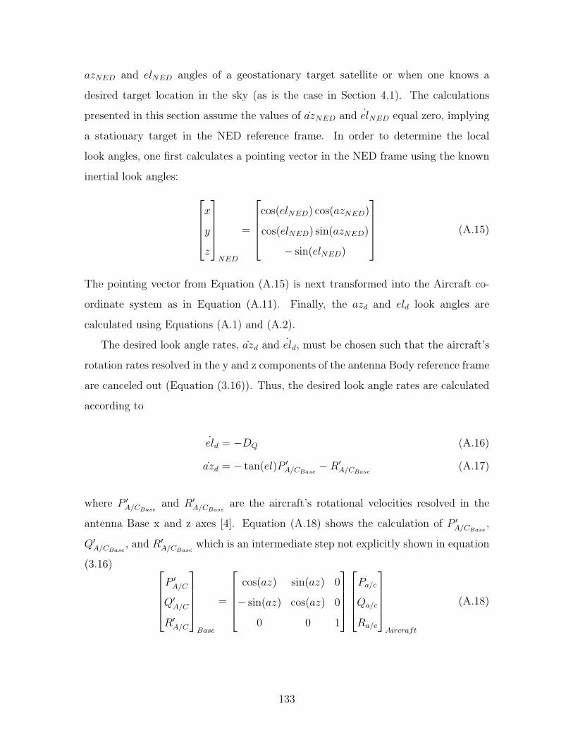
azNED and elNED angles of a geostationary target satellite or when one knows a
desired target location in the sky (as is the case in Section 4.1). The calculations
presented in this section assume the values of azNED and elNED equal zero, implying
a stationary target in the NED reference frame. In order to determine the local
look angles, one first calculates a pointing vector in the NED frame using the known
inertial look angles: x
y
z
NED
=
cos(elNED) cos(azNED)
cos(elNED) sin(azNED)
− sin(elNED)
(A.15)
The pointing vector from Equation (A.15) is next transformed into the Aircraft co-
ordinate system as in Equation (A.11). Finally, the azd and eld look angles are
calculated using Equations (A.1) and (A.2).
The desired look angle rates, azd and eld, must be chosen such that the aircraft’s
rotation rates resolved in the y and z components of the antenna Body reference frame
are canceled out (Equation (3.16)). Thus, the desired look angle rates are calculated
according to
eld = −DQ (A.16)
azd = − tan(el)P ′A/CBase −R′A/CBase
(A.17)
where P ′A/CBase and R′A/CBase are the aircraft’s rotational velocities resolved in the
antenna Base x and z axes [4]. Equation (A.18) shows the calculation of P ′A/CBase ,
Q′A/CBase , and R′A/CBase which is an intermediate step not explicitly shown in equation
(3.16) P ′A/C
Q′A/C
R′A/C
Base
=
cos(az) sin(az) 0
− sin(az) cos(az) 0
0 0 1
Pa/c
Qa/c
Ra/c
Aircraft
(A.18)
133
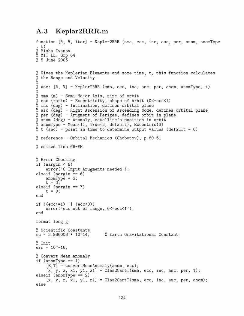
A.3 Keplar2RRR.m
function [R, V, iter] = Kepler2RRR (sma, ecc, inc, asc, per, anom, anomType, t)% Misha Ivanov% MIT LL, Grp 64% 5 June 2006
% Given the Keplerian Elements and some time, t, this function calculates% the Range and Velocity.%% use: [R, V] = Kepler2RRR (sma, ecc, inc, asc, per, anom, anomType, t)%% sma (m) - Semi-Major Axis, size of orbit% ecc (ratio) - Eccentricity, shape of orbit (0<=ecc<1)% inc (deg) - Inclination, defines orbital plane% asc (deg) - Right Ascension of Ascending Node, defines orbital plane% per (deg) - Arugment of Perigee, defines orbit in plane% anom (deg) - Anomaly, satellite’s position in orbit% anomType - Mean(1), True(2, default), Eccentric(3)% t (sec) - point in time to determine output values (default = 0)
% reference - Orbital Mechanics (Chobotov), p.60-61
% edited line 66-EM
% Error Checkingif (nargin < 6)
error(’6 Input Arugments needed’);elseif (nargin == 6)
anomType = 2;t = 0;
elseif (nargin == 7)t = 0;
end
if ((ecc>=1) || (ecc<0))error(’ecc out of range, 0<=ecc<1’);
end
format long g;
% Scientific Constantsmu = 3.986008 * 10^14; % Earth Gravitational Constant
% Initerr = 10^-16;
% Convert Mean anomalyif (anomType == 1)
[E,T] = convertMeanAnomaly(anom, ecc);[x, y, z, x1, y1, z1] = Clas2CartT(sma, ecc, inc, asc, per, T);
elseif (anomType == 2)[x, y, z, x1, y1, z1] = Clas2CartT(sma, ecc, inc, asc, per, anom);
else
134
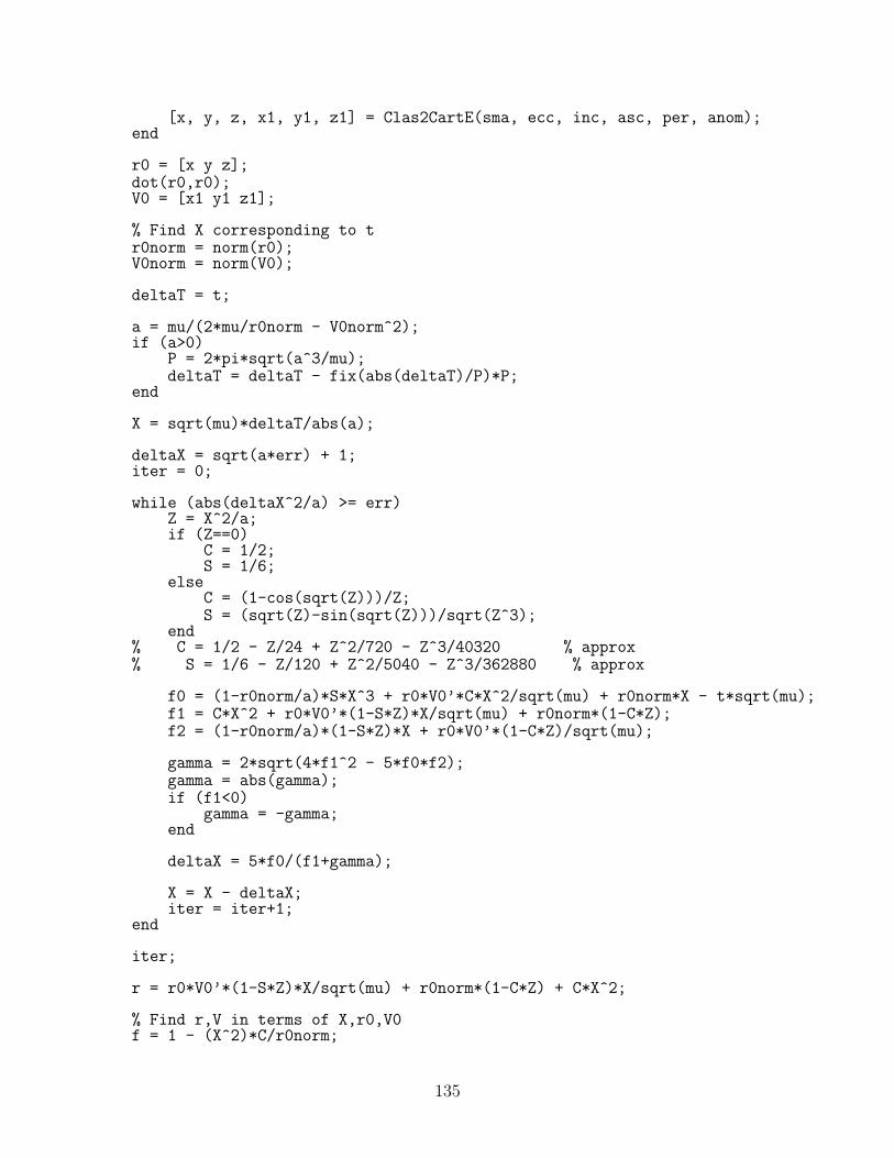
[x, y, z, x1, y1, z1] = Clas2CartE(sma, ecc, inc, asc, per, anom);end
r0 = [x y z];dot(r0,r0);V0 = [x1 y1 z1];
% Find X corresponding to tr0norm = norm(r0);V0norm = norm(V0);
deltaT = t;
a = mu/(2*mu/r0norm - V0norm^2);if (a>0)
P = 2*pi*sqrt(a^3/mu);deltaT = deltaT - fix(abs(deltaT)/P)*P;
end
X = sqrt(mu)*deltaT/abs(a);
deltaX = sqrt(a*err) + 1;iter = 0;
while (abs(deltaX^2/a) >= err)Z = X^2/a;if (Z==0)
C = 1/2;S = 1/6;
elseC = (1-cos(sqrt(Z)))/Z;S = (sqrt(Z)-sin(sqrt(Z)))/sqrt(Z^3);
end% C = 1/2 - Z/24 + Z^2/720 - Z^3/40320 % approx% S = 1/6 - Z/120 + Z^2/5040 - Z^3/362880 % approx
f0 = (1-r0norm/a)*S*X^3 + r0*V0’*C*X^2/sqrt(mu) + r0norm*X - t*sqrt(mu);f1 = C*X^2 + r0*V0’*(1-S*Z)*X/sqrt(mu) + r0norm*(1-C*Z);f2 = (1-r0norm/a)*(1-S*Z)*X + r0*V0’*(1-C*Z)/sqrt(mu);
gamma = 2*sqrt(4*f1^2 - 5*f0*f2);gamma = abs(gamma);if (f1<0)
gamma = -gamma;end
deltaX = 5*f0/(f1+gamma);
X = X - deltaX;iter = iter+1;
end
iter;
r = r0*V0’*(1-S*Z)*X/sqrt(mu) + r0norm*(1-C*Z) + C*X^2;
% Find r,V in terms of X,r0,V0f = 1 - (X^2)*C/r0norm;
135
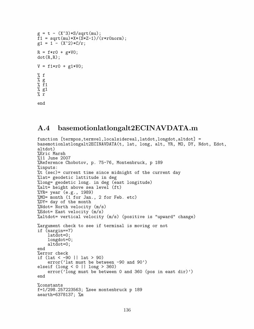
g = t - (X^3)*S/sqrt(mu);f1 = sqrt(mu)*X*(S*Z-1)/(r*r0norm);g1 = 1 - (X^2)*C/r;
R = f*r0 + g*V0;dot(R,R);
V = f1*r0 + g1*V0;
% f% g% f1% g1% r
end
A.4 basemotionlatlongalt2ECINAVDATA.m
function [termpos,termvel,localsidereal,latdot,longdot,altdot] =basemotionlatlongalt2ECINAVDATA(t, lat, long, alt, YR, MO, DY, Ndot, Edot,altdot)%Eric Marsh%11 June 2007%Reference Chobotov, p. 75-76, Montenbruck, p 189%inputs:%t (sec)= current time since midnight of the current day%lat= geodetic lattitude in deg%long= geodetic long. in deg (east longitude)%alt= height above sea level (ft)%YR= year (e.g., 1989)%MO= month (1 for Jan., 2 for Feb. etc)%DY= day of the month%Ndot= North velocity (m/s)%Edot= East velocity (m/s)%altdot= vertical velocity (m/s) (positive is "upward" change)
%argument check to see if terminal is moving or notif (nargin==7)
latdot=0;longdot=0;altdot=0;
end%error checkif (lat < -90 || lat > 90)
error(’lat must be between -90 and 90’)elseif (long < 0 || long > 360)
error(’long must be between 0 and 360 (pos in east dir)’)end
%constantsf=1/298.257223563; %see montenbruck p 189aearth=6378137; %m
136
wemin=0.2506844537; %earth’s rotation deg/minwerad=wemin*unitsratio(’rad’,’deg’)/60; %earth’s rotation rad/secwe=wemin/60; %earth’s rotation in deg/sec
%time calculationsalphamidnight=greenwichmidnight(YR,MO,DY); %greenwich angle at midnight%of sim daylocalsidereal=mod(long+alphamidnight+we*(t),360); %local sidereal time%angle at time ’t’
%convert inputslat=lat*unitsratio(’rad’,’deg’);localsidereal=localsidereal*unitsratio(’rad’,’deg’);alt=alt*unitsratio(’m’,’ft’);%altdot=altdot*unitsratio(’m’,’ft’); %m/s
%calculate terminal ECI coords (position vector and velocity vector)
%%%%%%%%%%%%%%Method derived from Montenbruck p 188)%%%%%%%%%%%%%%%%%%%%%N=aearth/sqrt(1-f*(2-f)*sin(lat)^2);x=(N+alt)*cos(lat)*cos(localsidereal);y=(N+alt)*cos(lat)*sin(localsidereal);z=((1-f)^2*N+alt)*sin(lat);termpos=[x y z]; %row of termpos vector gives x,y,z coord
%calculate velocity vector:%need latdot, longdot, altdot at every timelatdot=Ndot*(1/norm(termpos)); %North velocity to latdot (rad/s) conversions=cos(lat)*norm(termpos);longdot=Edot*(1/s); %East velocity to longdot (rad/s) conversion
Ndot=-(aearth/2)*(1-2*f*(sin(lat)^2)+f^2*sin(lat)^2)^(-3/2)*(-4*f*sin(lat)*cos(lat)*latdot+2*f^2*sin(lat)*cos(lat)*latdot);localsiderealdot=werad+longdot;xdot=Ndot*cos(lat)*cos(localsidereal)-N*sin(lat)*latdot*cos(localsidereal)-N*cos(lat)*sin(localsidereal)*localsiderealdot+altdot*cos(lat)*cos(localsidereal)-alt*sin(lat)*latdot*cos(localsidereal)-alt*cos(lat)*sin(localsidereal)*localsiderealdot;ydot=Ndot*cos(lat)*sin(localsidereal)-N*sin(lat)*latdot*sin(localsidereal)+N*cos(lat)*cos(localsidereal)*localsiderealdot+altdot*cos(lat)*sin(localsidereal)-alt*sin(lat)*latdot*sin(localsidereal)+alt*cos(lat)*cos(localsidereal)*localsiderealdot;zdot=((1-f)^2*Ndot*sin(lat)+(1-f)^2*N*cos(lat)*latdot+altdot*sin(lat)+alt*cos(lat)*latdot);termvel=[xdot ydot zdot];%%%%%%%%%%%%%%%%%%%%%%%%%%%%%%%%%%%%%%%%%%%
137

138
Appendix B
Open-Loop Controller Simulations
The following code was written using the MATLAB programming language, Version
7.4.0.287. It was run on a Dell laptop computer with a Pentium 4 processor, 2.13
GHz processor, and 2 GB of RAM using Microsoft Windows XP Professional, Version
2002 Service Pack 2.
B.1 controller.m
%Eric Marsh%MIT LL, Grp 61%February, 2008
%controller.m
%Description: This m-file develops the LQG controller for a nominal%Antenna Positioner System and simulates the performance using lsim. The%paramters needed for the Simulink model, ‘APSsimulinkmdl.mdl’ are included%at the end of this m-file.
clear all;close all;load Afilt;load Bfilt;
%plot PSD of filtersys=ss(Afilt,Bfilt,1,0);[mag,phase,w] = bode(sys);mag=squeeze(mag);db=20*log(mag);%figure;semilogx(w,db);xlabel(’freq (rad/s)’); ylabel(’DB mag’);%title(’Filter PSD’);
%inertia in el axis:
139
Iyy=635;%units are in^2*lbIyy=Iyy*0.4535924*0.0254^2;%convert to m^2*kgb=1/Iyy;
%motor constants:kaz=18.7; %oz-in/amp%kbaz=38.4; %V/10^3*RPMkaz=kaz*0.007061552; %N-m/amp%kbaz=kbaz*60/(2*pi)*10^-3; %Volts/(rad/sec)kbaz=kaz;raaz=4.84; %ohmskel=kaz;kbel=kbaz;rael=raaz;
%gearing:n=0.1; %n=r1/r2=radius of small gear/radius of large gear (m)
%reference input parameterN=1/0.005519215703220;
%state deriv left mult matrix:I=[Iyy 0 -Iyy; 0 1 0; 0 0 1];
A=zeros(3,3);A(1,1)=-kel*kbel/rael*(1/n^2);A(1,3)=kaz*kbaz/raaz*(1/n^2);A(2,1)=1;A(3,3)=Afilt;A=inv(I)*A;
Bu=zeros(3,1);Bu(1)=kel/rael*(1/n);Bu=inv(I)*Bu;
Bw=eye(3);Bw(3,3)=Bfilt;Bw=inv(I)*Bw;
Cy=[1 0 0; 0 1 0]; %sensing both velocity and position%Cy=[1 0 1]; %sensing just velocitcy Cy=[0 1 0]; %sensing just pos
%form controllability, observability matrices. can then check rank to see%if system is uncontrollable or unobservablessol=ss(A,Bu,Cy,0);ctol=ctrb(ssol);obol=obsv(ssol);
%LQR for control gains:% bryson’s rule for weighting Rxx: simply 1/(xmax)^2rxx(1)=1/(20*pi/180)^2;rxx(2)=1/(.01*pi/180)^2;rxx(3)=0; %zero weighting on filter stateRxx=diag(rxx);%Rxx=Rxx*10^9;Ruu=10^3; %control weighting[K,S,E]=lqr(A,Bu,Rxx,Ruu);
140
%LQR SimTs=0.01; %sim step sizetfinal=100; %sim end timet=0:Ts:tfinal;x0=[0;0;0]; %begin sim with a 3 deg/sec initial condition on velocityrho2=10^-7; %small amount of process noise (power spect. density??)Rww=diag([rho2,rho2,1]);%white noise input with unit variance on the filter%statew1=sqrt(Rww(1,1))*randn(length(t),1);w2=sqrt(Rww(2,2))*randn(length(t),1);Dp=sqrt(Rww(3,3)/Ts)*randn(length(t),1); %white noise disturbance input%to filter (divide by sqrt(Ts) to make pwr spectral density equal to 1)
Alqr=A-Bu*K;Bwlqr=[0;0;Bfilt];[y,x]=lsim(Alqr,Bw,Cy,0,[w1,w2,Dp],t,x0);% [y,x]=lsim(Alqr,Bwlqr,Cy,0,[Dp],t,x0);y=y*unitsratio(’deg’,’rad’);
%plots% figure;plot(t,y(:,1)); xlabel(’sim time (s)’); ylabel(’inertial rate% (deg/sec)’); legend(’antpitchdot’); title(’LQR with dist FF’);% figure;plot(t,y(:,2)); xlabel(’sim time (s)’); ylabel(’inertial angle% (deg)’); legend(’antpitch’); title(’LQR with dist FF’);
%LQE for estimator gains:Rvv=eye(2);Rvv(1,1)=10^-8; %sensor weighting on gyroRvv(2,2)=10^-6; %sensor weighting on position sensorf=1;Rvv=f*Rvv;[L,Q,F]=lqr(A’,Cy’,Bw*Rww*Bw’,Rvv);L=L’;
%LQG sim: (simulate plant and estimator together) see attached block%diagramAlqg=[A -Bu*K;L*Cy A-Bu*K-L*Cy];Blqg=[Bw zeros(3,2) Bu*N; zeros(3,3) L Bu*N];Clqg=[Cy zeros(2,3)]; %for measuring both velocity and positionDlqg=zeros(2,6); % dims are rows of Clqg x cols of Blqgsyslqg=ss(Alqg,Blqg,Clqg,Dlqg);
x0lqg=[x0; zeros(3,1)];v1=sqrt(10^-8)*randn(length(t),1); %white velocity sensor noisev2=sqrt(10^-6)*randn(length(t),1); %white position sensor noise%ref(:,1)=zeros(length(t),1);ref(:,1)=[zeros(101,1);ones(9900,1)*1*pi/180]; %step response
% ref(:,1)=[zeros(101,1);ones(9900,1)*0.16*pi/180];[ylqg,xlqg]=lsim(Alqg,Blqg,Clqg,Dlqg,[w1,w2,Dp,v1,v2,ref],t,x0lqg);%torque calcs:ulqgel(:,1)=-[zeros(1,3) K]*xlqg’+N*ref’; %input voltage to el motorilqgel=ulqgel/rael-(kbel/rael)*1/n*xlqg(:,1);torqueel=kel*ilqgel;%convert from N-m to oz-in:torqueel=torqueel*1/0.007061552;
141

ylqg=ylqg*unitsratio(’deg’,’rad’); %convert sim outputs to rad/sec and rad
%plots:% figure;plot(t,ylqg(:,1));hold all; plot(t,xlqg(:,4)*180/pi);hold off;% xlabel(’sim time (s)’); ylabel(’angle rate (deg/sec)’);% legend(’antpitchdot’,’Qdot estimate’); title(’LQG sim’);% figure;plot(t,ylqg(:,2));hold all; plot(t,xlqg(:,5)*180/pi);hold off;% xlabel(’sim time (s)’); ylabel(’angle (deg)’); legend(’antpitch’,’q% estimate’); title(’LQG sim’); figure;plot(t,xlqg(:,3)*180/pi);hold all;% plot(t,xlqg(:,6)*180/pi); hold off; xlabel(’sim time (s)’); ylabel(’dist% rate (deg/sec)’); legend(’antpitchdist’,’antpitchdist estimate’);% title(’dist input’); figure;plot(t,torqueel);hold all;plot([0 max(t)],[30% 30],’m--’); plot([0 max(t)],[-30 -30],’m--’);hold off; xlabel(’sim time% (s)’); ylabel(’torque (oz-in)’); legend(’elevation torque’); title(’El% Torque v. Time’); figure;bode(syslqg);%% %simulink params Ixx=1217; %units are in^2*lb% Ixx=Ixx*0.4535924*0.0254^2;%convert to m^2*kg a=1/Ixx; Izz=Iyy; c=1/Izz;% XEL_Gyro_BW=10000; %bandwidth in hz XEL_Gyro_Bias=0; %rad/sec% XEL_Gyro_Noise=10^-8; %noise = avg power or variance in (rad/sec)^2% XEL_IMU_Bias=0; %rad/sec XEL_IMU_Error=10^-6; %noise = avg power or% variance in (rad/sec)^2 XEL_IMU_BW=10000; %bandwidth in hz% XEL_IMU_sample_time=1/10; XEL_Veh_Pos_Command_Rate=1/1000;% EL_Gyro_BW=10000; %bandwidth in hz EL_Gyro_Bias=0; %rad/sec% EL_Gyro_Noise=10^-8; %noise = avg power or variance in (rad/sec)^2% EL_IMU_Bias=0; %rad/sec EL_IMU_Error=10^-6; %noise = avg power or% variance in (rad/sec)^2 EL_IMU_BW=10000; %bandwidth in hz% EL_IMU_sample_time=1/10; EL_Veh_Pos_Command_Rate=1/1000;% el_motor_noloadspeed=5500*2*pi/60; %no load speed in rad/sec% el_motor_stall_torque=30*0.007061552; %stall torque in N-m% az_motor_noloadspeed=5500*2*pi/60; %no load speed in rad/sec% az_motor_stall_torque=30*0.007061552; %stall torque in N-m
142
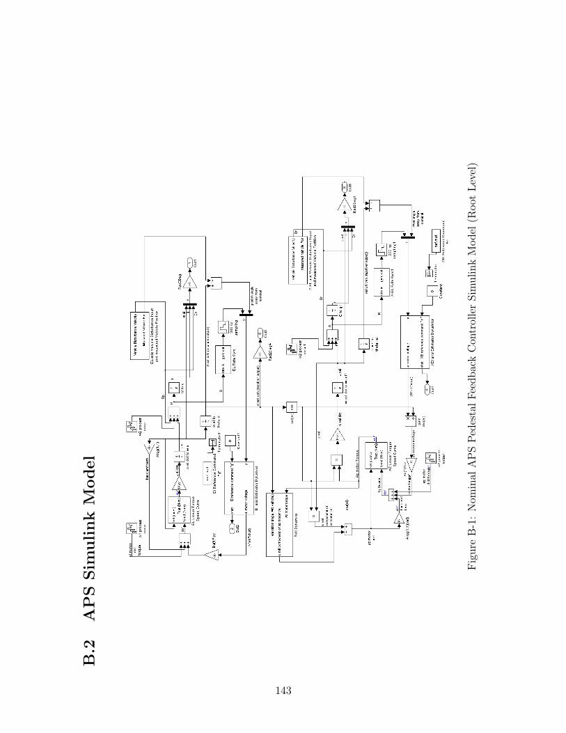
B.2
AP
SSim
ulink
Model
Fig
ure
B-1
:N
omin
alA
PS
Ped
esta
lF
eedbac
kC
ontr
olle
rSim
ulink
Model
(Root
Lev
el)
143
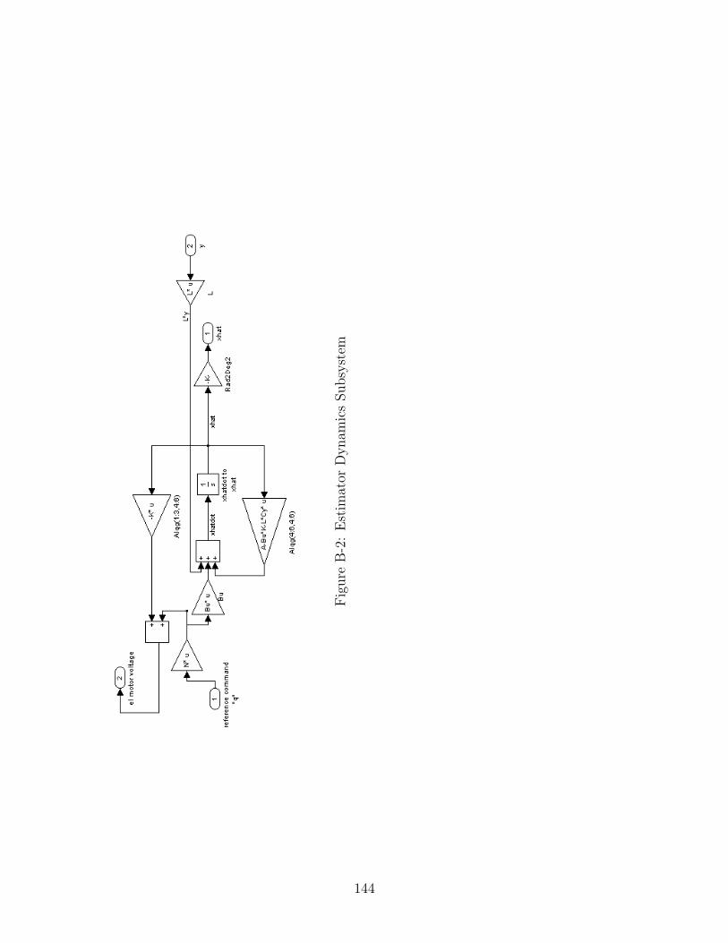
Fig
ure
B-2
:E
stim
ator
Dynam
ics
Subsy
stem
144
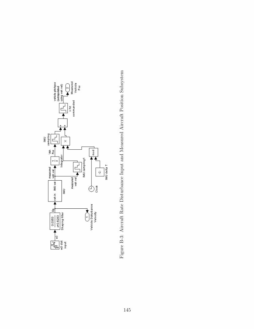
Fig
ure
B-3
:A
ircr
aft
Rat
eD
istu
rban
ceIn
put
and
Mea
sure
dA
ircr
aft
Pos
itio
nSubsy
stem
145
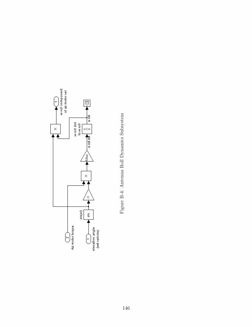
Fig
ure
B-4
:A
nte
nna
Rol
lD
ynam
ics
Subsy
stem
146
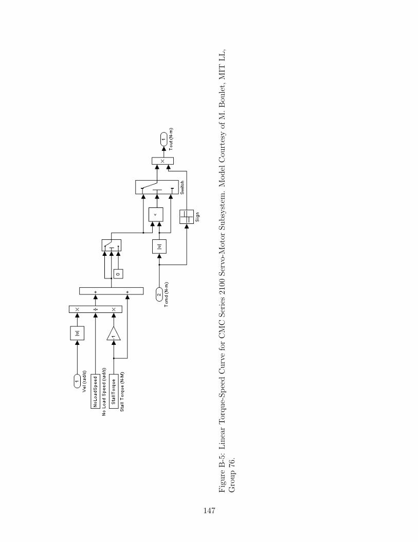
Fig
ure
B-5
:L
inea
rT
orque-
Sp
eed
Curv
efo
rC
MC
Ser
ies
2100
Ser
vo-M
otor
Subsy
stem
.M
odel
Cou
rtes
yof
M.
Bou
let,
MIT
LL
,G
roup
76.
147
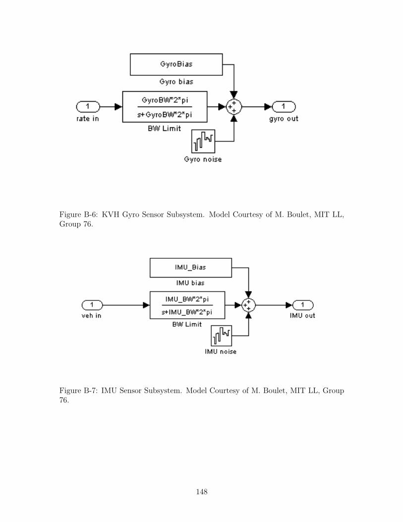
Figure B-6: KVH Gyro Sensor Subsystem. Model Courtesy of M. Boulet, MIT LL,Group 76.
Figure B-7: IMU Sensor Subsystem. Model Courtesy of M. Boulet, MIT LL, Group76.
148
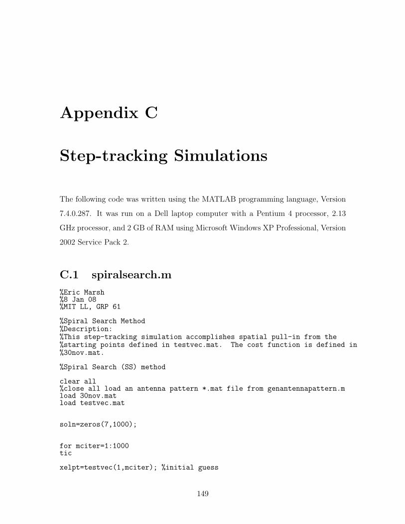
Appendix C
Step-tracking Simulations
The following code was written using the MATLAB programming language, Version
7.4.0.287. It was run on a Dell laptop computer with a Pentium 4 processor, 2.13
GHz processor, and 2 GB of RAM using Microsoft Windows XP Professional, Version
2002 Service Pack 2.
C.1 spiralsearch.m
%Eric Marsh%8 Jan 08%MIT LL, GRP 61
%Spiral Search Method%Description:%This step-tracking simulation accomplishes spatial pull-in from the%starting points defined in testvec.mat. The cost function is defined in%30nov.mat.
%Spiral Search (SS) method
clear all%close all load an antenna pattern *.mat file from genantennapattern.mload 30nov.matload testvec.mat
soln=zeros(7,1000);
for mciter=1:1000tic
xelpt=testvec(1,mciter); %initial guess
149
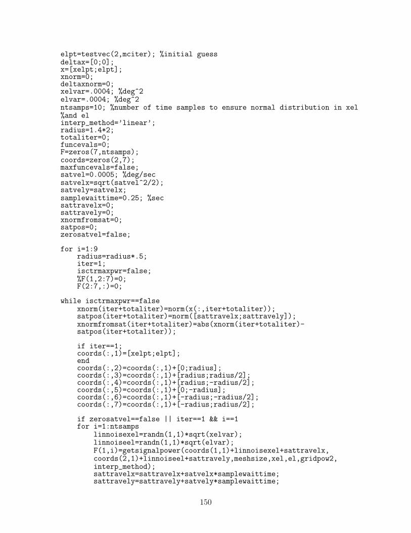
elpt=testvec(2,mciter); %initial guessdeltax=[0;0];x=[xelpt;elpt];xnorm=0;deltaxnorm=0;xelvar=.0004; %deg^2elvar=.0004; %deg^2ntsamps=10; %number of time samples to ensure normal distribution in xel%and elinterp_method=’linear’;radius=1.4*2;totaliter=0;funcevals=0;F=zeros(7,ntsamps);coords=zeros(2,7);maxfuncevals=false;satvel=0.0005; %deg/secsatvelx=sqrt(satvel^2/2);satvely=satvelx;samplewaittime=0.25; %secsattravelx=0;sattravely=0;xnormfromsat=0;satpos=0;zerosatvel=false;
for i=1:9radius=radius*.5;iter=1;isctrmaxpwr=false;%F(1,2:7)=0;F(2:7,:)=0;
while isctrmaxpwr==falsexnorm(iter+totaliter)=norm(x(:,iter+totaliter));satpos(iter+totaliter)=norm([sattravelx;sattravely]);xnormfromsat(iter+totaliter)=abs(xnorm(iter+totaliter)-satpos(iter+totaliter));
if iter==1;coords(:,1)=[xelpt;elpt];endcoords(:,2)=coords(:,1)+[0;radius];coords(:,3)=coords(:,1)+[radius;radius/2];coords(:,4)=coords(:,1)+[radius;-radius/2];coords(:,5)=coords(:,1)+[0;-radius];coords(:,6)=coords(:,1)+[-radius;-radius/2];coords(:,7)=coords(:,1)+[-radius;radius/2];
if zerosatvel==false || iter==1 && i==1for i=1:ntsamps
linnoisexel=randn(1,1)*sqrt(xelvar);linnoiseel=randn(1,1)*sqrt(elvar);F(1,i)=getsignalpower(coords(1,1)+linnoisexel+sattravelx,coords(2,1)+linnoiseel+sattravely,meshsize,xel,el,gridpow2,interp_method);sattravelx=sattravelx+satvelx*samplewaittime;sattravely=sattravely+satvely*samplewaittime;
150

endF(1,1)=mean(F(1,:));F(1,1)=roundn(F(1,1),-1); %round to nearest tenthsfuncevals=funcevals+1;
%F(1)=getsignalpower(coords(1,1),coords(2,1),meshsize,xel,el,gridpow2,i%nterp_method); funcevals=funcevals+1;endif zerosatvel==false || F(2,1)==0for i=1:ntsamps
linnoisexel=randn(1,1)*sqrt(xelvar);linnoiseel=randn(1,1)*sqrt(elvar);F(2,i)=getsignalpower(coords(1,2)+linnoisexel+sattravelx,coords(2,2)+linnoiseel+sattravely,meshsize,xel,el,gridpow2,interp_method);sattravelx=sattravelx+satvelx*samplewaittime;sattravely=sattravely+satvely*samplewaittime;
endF(2,1)=mean(F(2,:));F(2,1)=roundn(F(2,1),-1); %round to nearest tenthsfuncevals=funcevals+1;
%F(2)=getsignalpower(coords(1,2),coords(2,2),meshsize,xel,el,gridpow2,i%nterp_method); funcevals=funcevals+1;endif zerosatvel==false || F(3,1)==0for i=1:ntsamps
linnoisexel=randn(1,1)*sqrt(xelvar);linnoiseel=randn(1,1)*sqrt(elvar);F(3,i)=getsignalpower(coords(1,3)+linnoisexel+sattravelx,coords(2,3)+linnoiseel+sattravely,meshsize,xel,el,gridpow2,interp_method);sattravelx=sattravelx+satvelx*samplewaittime;sattravely=sattravely+satvely*samplewaittime;
endF(3,1)=mean(F(3,:));F(3,1)=roundn(F(3,1),-1); %round to nearest tenthsfuncevals=funcevals+1;
%F(3)=getsignalpower(coords(1,3),coords(2,3),meshsize,xel,el,gridpow2,i%nterp_method); funcevals=funcevals+1;endif zerosatvel==false || F(4,1)==0for i=1:ntsamps
linnoisexel=randn(1,1)*sqrt(xelvar);linnoiseel=randn(1,1)*sqrt(elvar);F(4,i)=getsignalpower(coords(1,4)+linnoisexel+sattravelx,coords(2,4)+linnoiseel+sattravely,meshsize,xel,el,gridpow2,interp_method);sattravelx=sattravelx+satvelx*samplewaittime;sattravely=sattravely+satvely*samplewaittime;
endF(4,1)=mean(F(4,:));F(4,1)=roundn(F(4,1),-1); %round to nearest tenthsfuncevals=funcevals+1;%F(4)=getsignalpower(coords(1,4),coords(2,4),meshsize,xel,el,gridpow2,i%nterp_method); funcevals=funcevals+1;
151
endif zerosatvel==false || F(5,1)==0for i=1:ntsamps
linnoisexel=randn(1,1)*sqrt(xelvar);linnoiseel=randn(1,1)*sqrt(elvar);F(5,i)=getsignalpower(coords(1,5)+linnoisexel+sattravelx,coords(2,5)+linnoiseel+sattravely,meshsize,xel,el,gridpow2,interp_method);sattravelx=sattravelx+satvelx*samplewaittime;sattravely=sattravely+satvely*samplewaittime;
endF(5,1)=mean(F(5,:));F(5,1)=roundn(F(5,1),-1); %round to nearest tenthsfuncevals=funcevals+1;%F(5)=getsignalpower(coords(1,5),coords(2,5),meshsize,xel,el,gridpow2,i%nterp_method); funcevals=funcevals+1;endif zerosatvel==false || F(6,1)==0for i=1:ntsamps
linnoisexel=randn(1,1)*sqrt(xelvar);linnoiseel=randn(1,1)*sqrt(elvar);F(6,i)=getsignalpower(coords(1,6)+linnoisexel+sattravelx,coords(2,6)+linnoiseel+sattravely,meshsize,xel,el,gridpow2,interp_method);sattravelx=sattravelx+satvelx*samplewaittime;sattravely=sattravely+satvely*samplewaittime;
endF(6,1)=mean(F(6,:));F(6,1)=roundn(F(6,1),-1); %round to nearest tenthsfuncevals=funcevals+1;%F(6)=getsignalpower(coords(1,6),coords(2,6),meshsize,xel,el,gridpow2,i%nterp_method); funcevals=funcevals+1;endif zerosatvel==false || F(7,1)==0for i=1:ntsamps
linnoisexel=randn(1,1)*sqrt(xelvar);linnoiseel=randn(1,1)*sqrt(elvar);F(7,i)=getsignalpower(coords(1,7)+linnoisexel+sattravelx,coords(2,7)+linnoiseel+sattravely,meshsize,xel,el,gridpow2,interp_method);sattravelx=sattravelx+satvelx*samplewaittime;sattravely=sattravely+satvely*samplewaittime;
endF(7,1)=mean(F(7,:));F(7,1)=roundn(F(7,1),-1); %round to nearest tenthsfuncevals=funcevals+1;%F(7)=getsignalpower(coords(1,7),coords(2,7),meshsize,xel,el,gridpow2,i%nterp_method); funcevals=funcevals+1;end
[C,I]=min(F(:,1));
Fcent=F(I,1);
if abs(satvel) < 10000*eps %saying if satvel is zero, can save some%function evaluationszerosatvel=true;
152
if I==2F(4,1)=F(3,1);F(5,1)=F(1,1);F(6,1)=F(7,1);F(2,1)=0;F(3,1)=0;F(7,1)=0;
elseif I==3F(5,1)=F(4,1);F(6,1)=F(1,1);F(7,1)=F(2,1);F(2,1)=0;F(3,1)=0;F(4,1)=0;
elseif I==4F(6,1)=F(5,1);F(7,1)=F(1,1);F(2,1)=F(3,1);F(3,1)=0;F(4,1)=0;F(5,1)=0;
elseif I==5F(7,1)=F(6,1);F(2,1)=F(1,1);F(3,1)=F(4,1);F(4,1)=0;F(5,1)=0;F(6,1)=0;
elseif I==6F(2,1)=F(7,1);F(3,1)=F(1,1);F(4,1)=F(5,1);F(5,1)=0;F(6,1)=0;F(7,1)=0;
elseif I==7F(3,1)=F(2,1);F(4,1)=F(1,1);F(5,1)=F(6,1);F(2,1)=0;F(6,1)=0;F(7,1)=0;
elseisctrmaxpwr=true;
endelseif I ==1
isctrmaxpwr=true;end
coords(:,1)=coords(:,I);F(1,1)=Fcent;
x(:,iter+1+totaliter)=coords(:,1);deltax(:,iter+totaliter)=x(:,iter+1+totaliter)-x(:,iter+totaliter);deltaxnorm(:,iter+totaliter)=norm(deltax(:,iter+totaliter));iter=iter+1;if funcevals > 500
maxfuncevals=true;warning(’max number of function evaluations reached’)
153

breakend
endxelpt=coords(1,1);elpt=coords(2,1);totaliter=totaliter+iter-1;if maxfuncevals==true %break for loop if maxfuncevals is true
breakend
end
%calculate approximate timeif satvel > eps*10000 %if satvel isn’t zero
time=satpos(end)/satvel;else
time=0;endsoln(1:2,mciter)=[x(1,end);x(2,end)];soln(3,mciter)=totaliter;simtime=toc;soln(4,mciter)=simtime;soln(5,mciter)=funcevals;soln(6,mciter)=xnorm(end);soln(7,mciter)=satpos(end);soln(8,mciter)=xnormfromsat(end);soln(9,mciter)=time;
end
C.2 modifiedNewton.m
%Eric Marsh 18 Dec 07
%Modified Newton’s Method%Description:%This step-tracking simulation accomplishes spatial pull-in from the%starting points defined in testvec.mat. The cost function is defined in%30nov.mat.
clear all%close all load an antenna pattern *.mat file from genantennapattern.mload 30nov.matload testvec.mat
soln=zeros(7,1000);mainlobejump=zeros(1,1000);bracketminfalse=zeros(1,1000);gradfalloffcount=zeros(1,1000);
for mciter=1:1000ticxelpt=testvec(1,mciter); %initial guesselpt=testvec(2,mciter); %initial guess
154

deljstep=.16; %(deg) this is ~3* the 3sigma on the 1-d pointing error%distributions (also good for lin interp of ant pattern and machine errors)deltax=[0;0];x=[xelpt;elpt];xnorm=0;deltaxnorm=0;iter=1;epsilon=0.63; %looser?gradient=[10^2;10^2];hessian=zeros(2,2);interp_method=’linear’;R=zeros(2,2);funcevals=0;xelvar=.0004; %deg^2elvar=.0004; %deg^2ntsamps=10; %number of time samples to ensure normal distribution in xel%and elFminjump=zeros(1,ntsamps);gradswitch=epsilon*10;linsearchparam=0.5;linstepcount=0;mincheck=0;mincheckthreshold=4;hessianhat=zeros(2,2);directedgrad=0;mincheckvec=0;gradfalloff=0;satvel=0.0005; %deg/secsatvelx=sqrt(satvel^2/2);satvely=satvelx;samplewaittime=0.25; %secsattravelx=0;sattravely=0;xnormfromsat=0;satpos=0;
% set terminate = falseterminate=false;% while terminate = falsewhile terminate==false% set compute alpha*pk = truecomputedeltax=true;%perform function/gradient evaluations at xk: initializationsxnorm(iter)=norm(x(:,iter));satpos(iter)=norm([sattravelx;sattravely]);xnormfromsat(iter)=abs(xnorm(iter)-satpos(iter));F=zeros(13,ntsamps);g=zeros(2,5);G=zeros(2,2);
%%%%%%%%%%%%%%%%%%%%%%%%%%%%%perform function evals:%%%%%%%%%%%%%%%%%%%%%%%noisexel=randn(14,ntsamps)*sqrt(xelvar); %14th pt is for jump conditionnoiseel=randn(14,ntsamps)*sqrt(elvar);
%F9,F10,F11 not needed
if Fminjump(1)==0
155
computeF1=true;else
computeF1=false;end%%%F1%%%if computeF1==truefor i=1:ntsamps
linnoisexel=randn(1,1)*sqrt(xelvar);linnoiseel=randn(1,1)*sqrt(elvar);F(1,i)=getsignalpower(xelpt+linnoisexel+sattravelx,elpt+linnoiseel+sattravely,meshsize,xel,el,gridpow2,interp_method);sattravelx=sattravelx+satvelx*samplewaittime;sattravely=sattravely+satvely*samplewaittime;
endF(1,1)=mean(F(1,:));F(1,1)=roundn(F(1,1),-1); %round to nearest tenthsfuncevals=funcevals+1;else
F(1,1)=Fminjump(1);end
%%%F2%%%for i=1:ntsamps
linnoisexel=randn(1,1)*sqrt(xelvar);linnoiseel=randn(1,1)*sqrt(elvar);F(2,i)=getsignalpower(xelpt+linnoisexel+deljstep+sattravelx,elpt+linnoiseel+sattravely,meshsize,xel,el,gridpow2,interp_method);sattravelx=sattravelx+satvelx*samplewaittime;sattravely=sattravely+satvely*samplewaittime;
endF(2,1)=mean(F(2,:));F(2,1)=roundn(F(2,1),-1); %round to nearest tenthsfuncevals=funcevals+1;
%%%F5%%%for i=1:ntsamps
linnoisexel=randn(1,1)*sqrt(xelvar);linnoiseel=randn(1,1)*sqrt(elvar);F(5,i)=getsignalpower(xelpt+linnoisexel+sattravelx,elpt+linnoiseel+deljstep+sattravely,meshsize,xel,el,gridpow2,interp_method);sattravelx=sattravelx+satvelx*samplewaittime;sattravely=sattravely+satvely*samplewaittime;
endF(5,1)=mean(F(5,:));F(5,1)=roundn(F(5,1),-1); %round to nearest tenthsfuncevals=funcevals+1;
%%%F6%%%for i=1:ntsamps
linnoisexel=randn(1,1)*sqrt(xelvar);linnoiseel=randn(1,1)*sqrt(elvar);F(6,i)=getsignalpower(xelpt+linnoisexel+deljstep+sattravelx,elpt+linnoiseel+deljstep+sattravely,meshsize,xel,el,gridpow2,interp_method);sattravelx=sattravelx+satvelx*samplewaittime;sattravely=sattravely+satvely*samplewaittime;
endF(6,1)=mean(F(6,:));F(6,1)=roundn(F(6,1),-1); %round to nearest tenths
156

funcevals=funcevals+1;
%%%F7%%%for i=1:ntsamps
linnoisexel=randn(1,1)*sqrt(xelvar);linnoiseel=randn(1,1)*sqrt(elvar);F(7,i)=getsignalpower(xelpt+linnoisexel+2*deljstep+sattravelx,elpt+linnoiseel+sattravely,meshsize,xel,el,gridpow2,interp_method);sattravelx=sattravelx+satvelx*samplewaittime;sattravely=sattravely+satvely*samplewaittime;
endF(7,1)=mean(F(7,:));F(7,1)=roundn(F(7,1),-1); %round to nearest tenthsfuncevals=funcevals+1;
%%%F13%%%for i=1:ntsamps
linnoisexel=randn(1,1)*sqrt(xelvar);linnoiseel=randn(1,1)*sqrt(elvar);F(13,i)=getsignalpower(xelpt+linnoisexel+sattravelx,elpt+linnoiseel+2*deljstep+sattravely,meshsize,xel,el,gridpow2,interp_method);sattravelx=sattravelx+satvelx*samplewaittime;sattravely=sattravely+satvely*samplewaittime;
endF(13,1)=mean(F(13,:));F(13,1)=roundn(F(13,1),-1); %round to nearest tenthsfuncevals=funcevals+1;
if iter==1 || norm(gradient(:,iter-1)) < gradswitch%%%F3%%%for i=1:ntsamps
linnoisexel=randn(1,1)*sqrt(xelvar);linnoiseel=randn(1,1)*sqrt(elvar);F(3,i)=getsignalpower(xelpt+linnoisexel+sattravelx,elpt+linnoiseel-deljstep+sattravely,meshsize,xel,el,gridpow2,interp_method);sattravelx=sattravelx+satvelx*samplewaittime;sattravely=sattravely+satvely*samplewaittime;
endF(3,1)=mean(F(3,:));F(3,1)=roundn(F(3,1),-1); %round to nearest tenthsfuncevals=funcevals+1;
%%%F4%%%for i=1:ntsamps
linnoisexel=randn(1,1)*sqrt(xelvar);linnoiseel=randn(1,1)*sqrt(elvar);F(4,i)=getsignalpower(xelpt+linnoisexel-deljstep+sattravelx,elpt+linnoiseel+sattravely,meshsize,xel,el,gridpow2,interp_method);sattravelx=sattravelx+satvelx*samplewaittime;sattravely=sattravely+satvely*samplewaittime;
endF(4,1)=mean(F(4,:));F(4,1)=roundn(F(4,1),-1); %round to nearest tenthsfuncevals=funcevals+1;
%%%F8%%%for i=1:ntsamps
157
linnoisexel=randn(1,1)*sqrt(xelvar);linnoiseel=randn(1,1)*sqrt(elvar);F(8,i)=getsignalpower(xelpt+linnoisexel+deljstep+sattravelx,elpt+linnoiseel-deljstep+sattravely,meshsize,xel,el,gridpow2,interp_method);sattravelx=sattravelx+satvelx*samplewaittime;sattravely=sattravely+satvely*samplewaittime;
endF(8,1)=mean(F(8,:));F(8,1)=roundn(F(8,1),-1); %round to nearest tenthsfuncevals=funcevals+1;
%%%F12%%%for i=1:ntsamps
linnoisexel=randn(1,1)*sqrt(xelvar);linnoiseel=randn(1,1)*sqrt(elvar);F(12,i)=getsignalpower(xelpt+linnoisexel-deljstep+sattravelx,elpt+linnoiseel+deljstep+sattravely,meshsize,xel,el,gridpow2,interp_method);sattravelx=sattravelx+satvelx*samplewaittime;sattravely=sattravely+satvely*samplewaittime;
endF(12,1)=mean(F(12,:));F(12,1)=roundn(F(12,1),-1); %round to nearest tenthsfuncevals=funcevals+1;endFminjump=zeros(1,ntsamps);
%%%%old way%%%%%%%%%%%%%%%%%%%%%%%%%%%%%%%%%%%%%%%%%%%%%%%%%%% if Fminjump(1)==0% computeF1=true;% else% computeF1=false;% end for i=1:ntsamps if computeF1 == true% F(1,i)=getsignalpower(xelpt+noisexel(1,i),elpt+noiseel(1,i),meshsize,xel,% el,gridpow2,interp_method); else% F(1,i)=Fminjump(1);% end% F(2,i)=getsignalpower(xelpt+noisexel(2,i)+deljstep,elpt+noiseel(2,i),mesh% size,xel,el,gridpow2,interp_method);% F(5,i)=getsignalpower(xelpt+noisexel(5,i),elpt+noiseel(5,i)+deljstep,mesh% size,xel,el,gridpow2,interp_method);% F(6,i)=getsignalpower(xelpt+noisexel(6,i)+deljstep,elpt+noiseel(6,i)+delj% step,meshsize,xel,el,gridpow2,interp_method);% F(7,i)=getsignalpower(xelpt+noisexel(7,i)+2*deljstep,elpt+noiseel(7,i),me% shsize,xel,el,gridpow2,interp_method);% F(13,i)=getsignalpower(xelpt+noisexel(13,i),elpt+noiseel(13,i)+2*deljstep% ,meshsize,xel,el,gridpow2,interp_method); if iter==1 ||% norm(gradient(:,iter-1)) < gradswitch% F(3,i)=getsignalpower(xelpt+noisexel(3,i),elpt+noiseel(3,i)-deljstep,mesh% size,xel,el,gridpow2,interp_method);% F(4,i)=getsignalpower(xelpt+noisexel(4,i)-deljstep,elpt+noiseel(4,i),mesh% size,xel,el,gridpow2,interp_method);% F(8,i)=getsignalpower(xelpt+noisexel(8,i)+deljstep,elpt+noiseel(8,i)-delj% step,meshsize,xel,el,gridpow2,interp_method);% F(12,i)=getsignalpower(xelpt+noisexel(12,i)-deljstep,elpt+noiseel(12,i)+d% eljstep,meshsize,xel,el,gridpow2,interp_method); end end for i=1:13% %average the signal to noise measurements and store in first column of F
158

% F(i,1)=mean(F(i,:)); end Fminjump=zeros(1,ntsamps); F=roundn(F,-1);% %round to nearest tenths%calculate number of points looked at (function evaluations):% if computeF1==true% if iter==1 || norm(gradient(:,iter-1)) < gradswitch% funcevals=funcevals+10;% else% funcevals=funcevals+6;% end% else% if iter==1 || norm(gradient(:,iter-1)) < gradswitch% funcevals=funcevals+9;% else% funcevals=funcevals+5;% end% end%%%%%%%%%%%%%%%%%%%%%%%%%%%%%%%%%%%%%%%%%%%%%%%%%%%%%%%%%%%%%%%
%Form gradient vectors g3,g4 not neededif iter==1 || norm(gradient(:,iter-1)) < gradswitch
g(:,1)=[(F(2,1)-F(4,1))/(2*deljstep);(F(5,1)-F(3,1))/(2*deljstep)];gradient(:,iter)=g(:,1);g(:,2)=[(F(7,1)-F(1,1))/(2*deljstep);(F(6,1)-F(8,1))/(2*deljstep)];%g(:,3)=[(F(8,1)-F(10,1))/(2*deljstep);(F(1,1)-F(9,1))/(2*deljstep)];%g(:,4)=[(F(1,1)-F(11,1))/(2*deljstep);(F(12,1)-F(10,1))/(2*deljstep)];g(:,5)=[(F(6,1)-F(12,1))/(2*deljstep);(F(13,1)-F(1,1))/(2*deljstep)];
elseg(:,1)=[(F(2,1)-F(1,1))/(deljstep);(F(5,1)-F(1,1))/(deljstep)];gradient(:,iter)=g(:,1);fwddifcount(iter)=1;g(:,2)=[(F(7,1)-F(2,1))/(deljstep);(F(6,1)-F(2,1))/(deljstep)];g(:,5)=[(F(6,1)-F(5,1))/(deljstep);(F(13,1)-F(5,1))/(deljstep)];
end
%form hessian (G) matrixG(:,1)=(g(:,2)-g(:,1))/(deljstep);G(:,2)=(g(:,5)-g(:,1))/(deljstep);G=.5*(G+G’);hessian(:,:,iter)=G;%modified cholesky factorization of HessianL=eye(2);D=zeros(2,2);R=zeros(2,2);delta=10; %50; %10^1 good? %effectively adds more damping to lin searchfor j=1:2
if j==1D(j,j)=G(j,j);if D(j,j)<delta
R(j,j)=(delta-D(j,j));D(j,j)=R(j,j)+D(j,j);
endL(2,j)=G(2,j)/D(j,j);
elseif j==2D(j,j)=G(j,j)-D(1,1)*(L(j,1))^2;if D(j,j)<delta
R(j,j)=(delta-D(j,j));
159
D(j,j)=R(j,j)+D(j,j);end
endend%%%%%%%%hessianhat(:,:,iter)=L*D*L’;t(:,iter)=L\-gradient(:,iter);rhs=inv(D)*t(:,iter);
%%%%%%%%%%%%%%%%%%%%%%%%check for local or global min:%%%%%%%%%%%%%%%%%%%%%% if criteria for minimum = true (small gradient)if norm(gradient(:,iter)) < epsilon
%check for local minif (norm(gradient(:,iter))<epsilon) && (R(1,1) > 0 || R(2,2) > 0) %if
%you’re at a weak min (grad small, hessian modified)V=zeros(2,2);E=zeros(2,2);deltaxminjump=zeros(2,1);jumpxel=0;jumpel=0;[V,E]=eig(hessian(:,:,iter));if V(:,1)’*hessian(:,:,iter)*V(:,1) > V(:,2)’*hessian(:,:,iter)*
V(:,2)deltaxminjump=V(:,1);
elsedeltaxminjump=V(:,2);
enddeltaxminjump=deltaxminjump*1.85; %1.85 comes from averagingdistance between first 4 peaks on ant. patternjumpxel=x(1,iter)+deltaxminjump(1);jumpel=x(2,iter)+deltaxminjump(2);for i=1:ntsamps
linnoisexel=randn(1,1)*sqrt(xelvar);linnoiseel=randn(1,1)*sqrt(elvar);Fminjump(i)=getsignalpower(jumpxel+linnoisexel+sattravelx,jumpel+linnoiseel+sattravely,meshsize,xel,el,gridpow2,interp_method);sattravelx=sattravelx+satvelx*samplewaittime;sattravely=sattravely+satvely*samplewaittime;
endFminjump(1)=mean(Fminjump(1,:));Fminjump=roundn(Fminjump(1),-1); %round to nearest tenthsfuncevals=funcevals+1;if Fminjump(1) > F(1,1) %must check to see you are going in right
%direction on eigenvectordeltax(:,iter)=deltaxminjump*-1; %head the opposite wayFminjump(1)=0;
elsedeltax(:,iter)=deltaxminjump; %you jumped the correct way
endmincheck=0;
elsedeltax(:,iter)=[0;0];mincheck=mincheck+1;
endcomputedeltax=false;
160
if mincheck > mincheckthreshold%computedeltax=true; %complete one more jump (already evaluated the%function so might as well)terminate=true;
endelseif mincheck > 0 && norm(gradient(:,iter)) > epsilon
computedeltax=true;mincheck=0;gradfalloff(iter)=1;
endmincheckvec(iter)=mincheck;
if computedeltax==true %%%%%%%%%%%if compute alpha*pk = true%%%%%%%%%%%%
%%%%%%%%%compute pk and initial alpha:%%%%%%%%%%%%%%%%%%%%%%deltax(:,iter)=L’\rhs;alpha=1;%limit alpha*pk to a predetermined region of confidence:if norm(deltax(:,iter))>1.0 %if deltax is outside a "region of trust"
%chosen so if you’re at a max, won’t go over another max (max initial%step routine will take)deltax(:,iter)=(deltax(:,iter)/norm(deltax(:,iter)))*.75;
end
%evaluate function at initial alpha=1 value:for i=1:ntsamps
linnoisexel=randn(1,1)*sqrt(xelvar);linnoiseel=randn(1,1)*sqrt(elvar);Falpha(i)=getsignalpower(x(1,iter)+deltax(1,iter)+linnoisexel+sattravelx,x(2,iter)+deltax(2,iter)+linnoiseel+sattravely,meshsize,xel,el,gridpow2,interp_method);sattravelx=sattravelx+satvelx*samplewaittime;sattravely=sattravely+satvely*samplewaittime;
endFalpha(1)=mean(Falpha(1,:));Falpha=roundn(Falpha(1),-1); %round to nearest tenthsfuncevals=funcevals+1;
%evaluate point along search direction to approximate gradient at alpha=1dx1=deltax(1,iter)/norm(deltax(:,iter));dx2=deltax(2,iter)/norm(deltax(:,iter));nux=dx1*deljstep;nuy=dx2*deljstep;if norm([alpha*deltax(1,iter);alpha*deltax(2,iter)])>=deljstep
if alpha > 0nu=norm([alpha*deltax(1,iter)-nux;alpha*deltax(2,iter)-nuy])/norm(deltax(:,iter)); %ensure that nu value will be deljstep away%from alpha in 1-d
elsenu=-1*norm([alpha*deltax(1,iter)+nux;alpha*deltax(2,iter)+nuy])/norm(deltax(:,iter));
endelse
if alpha > 0nu=-1*norm([alpha*deltax(1,iter)-nux;alpha*deltax(2,iter)-nuy])/
161
norm(deltax(:,iter)); %ensure that nu value will be deljstep away%from alpha in 1-d
elsenu=norm([alpha*deltax(1,iter)+nux;alpha*deltax(2,iter)+nuy])/norm(deltax(:,iter));
endendfor i=1:ntsamps
linnoisexel=randn(1,1)*sqrt(xelvar);linnoiseel=randn(1,1)*sqrt(elvar);Fnu(i)=getsignalpower(x(1,iter)+nu*deltax(1,iter)+linnoisexel+sattravelx,x(2,iter)+nu*deltax(2,iter)+linnoiseel+sattravely,meshsize,xel,el,gridpow2,interp_method);sattravelx=sattravelx+satvelx*samplewaittime;sattravely=sattravely+satvely*samplewaittime;
endFnu(1)=mean(Fnu(1,:));Fnu=roundn(Fnu(1),-1); %round to nearest tenthsfuncevals=funcevals+1;
%%%%%%%%%%%%%%%%%%%%perform linear search along pk to determine%%%%%%%%%%%%%%%%%%%%satisfactory alpha %%%%%%%%%%%%%%%%%%%%%%linsearchconverge=false;directedgrad(iter)=deltax(:,iter)’*gradient(:,iter);%if alpha=1 is not satisfactory, perform lin search:if abs((Falpha-Fnu))/deljstep > abs(-1*linsearchparam*directedgrad(iter))
%Criterion for lin search-(finite difference replaces gradient)- GMW%p. 102
%Step 1- make sure you have an interval bracketing a minimum:bracketmin=true;if F(1,1)<Falpha %look opposite direction to find Fa and a values for
%interval containing minimumalpha=-1;bracket_step=1;Fb=Falpha;b=1;Fc=F(1,1);c=0;Fa=-10^6;a=alpha;
while Fa(1) <= Fcif bracket_step > 1
Fb=Fc;b=c;Fc=Fa(1);c=a;
endfor i=1:ntsamps
linnoisexel=randn(1,1)*sqrt(xelvar);linnoiseel=randn(1,1)*sqrt(elvar);Fa(i)=getsignalpower(x(1,iter)+alpha*deltax(1,iter)+linnoisexel+sattravelx,x(2,iter)+alpha*deltax(2,iter)+linnoiseel+sattravely,meshsize,xel,el,gridpow2,interp_method);sattravelx=sattravelx+satvelx*samplewaittime;sattravely=sattravely+satvely*samplewaittime;
162
endFa(1)=mean(Fa(1,:));Fa=roundn(Fa(1),-1); %round to nearest tenthsfuncevals=funcevals+1;a=alpha;alpha=alpha*2;bracket_step=bracket_step+1;
if bracket_step > 4bracketmin=false;bracketminfalse(mciter)=bracketminfalse(mciter)+1;warning(’could not bracket minimum for lin search in lessthan 4 steps’)break
endend
else %continue searching along search direction until a min is%bracketed- (find b)
alpha=2;bracket_step=1;Fc=Falpha;c=1;Fa=F(1,1);a=0;Fb=-10^6;b=alpha;
while Fb(1) <= Fcif bracket_step > 1
Fa=Fc;a=c;Fc=Fb(1);c=b;
end
for i=1:ntsampslinnoisexel=randn(1,1)*sqrt(xelvar);linnoiseel=randn(1,1)*sqrt(elvar);Fb(i)=getsignalpower(x(1,iter)+alpha*deltax(1,iter)+linnoisexel+sattravelx,x(2,iter)+alpha*deltax(2,iter)+linnoiseel+sattravely,meshsize,xel,el,gridpow2,interp_method);sattravelx=sattravelx+satvelx*samplewaittime;sattravely=sattravely+satvely*samplewaittime;
endFb(1)=mean(Fb(1,:));Fb=roundn(Fb(1),-1); %round to nearest tenthsfuncevals=funcevals+1;b=alpha;alpha=alpha*2-1;bracket_step=bracket_step+1;
if bracket_step > 4bracketmin=false;bracketminfalse(mciter)=bracketminfalse(mciter)+1;warning(’could not bracket minimum for lin search in lessthan 4 steps’)break
endend
end
163
%Step 2- perform quadradic interpolation:if bracketmin==true %lin search...
linsearchconverge=true;linstep=1;while linstep==1 || abs((Falpha-Fnu))/deljstep > abs(-1*
linsearchparam*directedgrad(iter)) %criterion for linear%search (finite difference replaces gradient)- GMW p. 102if linstep > 1
if alpha < c && Falpha <= Fcb=c;c=alpha;Fb=Fc;Fc=Falpha;
elseif alpha > c && Falpha > Fcb=alpha;Fb=Falpha;
elseif alpha < c && Falpha > Fca=alpha;Fa=Falpha;
elsea=c;c=alpha;Fa=Fc;Fc=Falpha;
endendif Fa==Fb && Fb==Fc %can’t optimize any further with quad interp
breakendif c-10000*eps<a&&a<c+10000*eps %saying if a==c
%can’t optimize any further with quad interpbreak
endif -10000*eps<((b-c)*Fa+(c-a)*Fb+(a-b)*Fc)&&((b-c)*Fa+(c-a)*
Fb+(a-b)*Fc)<10000*eps %saying if den of alpha calc == 0%can’t optimize any further with quad interpbreak
endalpha=.5*((b^2-c^2)*Fa+(c^2-a^2)*Fb+(a^2-b^2)*Fc)/((b-c)*Fa+(c-a)*Fb+(a-b)*Fc);for i=1:ntsamps
linnoisexel=randn(1,1)*sqrt(xelvar);linnoiseel=randn(1,1)*sqrt(elvar);Falpha(i)=getsignalpower(x(1,iter)+alpha*deltax(1,iter)+linnoisexel+sattravelx,x(2,iter)+alpha*deltax(2,iter)+linnoiseel+sattravely,meshsize,xel,el,gridpow2,interp_method);sattravelx=sattravelx+satvelx*samplewaittime;sattravely=sattravely+satvely*samplewaittime;
endFalpha(1)=mean(Falpha(1,:));Falpha=roundn(Falpha(1),-1); %round to nearest tenthsfuncevals=funcevals+1;if norm([alpha*deltax(1,iter);alpha*deltax(2,iter)])>=deljstep
if alpha > 0nu=norm([alpha*deltax(1,iter)-nux;alpha*deltax(2,iter)
-nuy])/norm(deltax(:,iter)); %ensure that nu value
164

%will be deljstep away from alpha in 1-delse
nu=-1*norm([alpha*deltax(1,iter)+nux;alpha*deltax(2,iter)+nuy])/norm(deltax(:,iter));
endelse
if alpha > 0nu=-1*norm([alpha*deltax(1,iter)-nux;alpha*
deltax(2,iter)-nuy])/norm(deltax(:,iter)); %ensure%that nu value will be deljstep away from alpha in 1-d
elsenu=norm([alpha*deltax(1,iter)+nux;alpha*deltax(2,iter)+
nuy])/norm(deltax(:,iter));end
endfor i=1:ntsamps
linnoisexel=randn(1,1)*sqrt(xelvar);linnoiseel=randn(1,1)*sqrt(elvar);Fnu(i)=getsignalpower(x(1,iter)+nu*deltax(1,iter)+linnoisexel+sattravelx,x(2,iter)+nu*deltax(2,iter)+linnoiseel+sattravely,meshsize,xel,el,gridpow2,interp_method);sattravelx=sattravelx+satvelx*samplewaittime;sattravely=sattravely+satvely*samplewaittime;
endFnu(1)=mean(Fnu(1,:));Fnu=roundn(Fnu(1),-1); %round to nearest tenthsfuncevals=funcevals+1;linstep=linstep+1;if linstep > 20
linsearchconverge=false;break
endendlinstepcount(iter)=linstep;
endendif linsearchconverge==true %if lin search produced a good alpha
%within max number of linstepsdeltax(:,iter)=deltax(:,iter)*alpha;
end %else, alpha remains at one (or whatever it was from the%minimum check routine)enddeltaxnorm(iter)=norm(deltax(:,iter));x(:,iter+1)=x(:,iter)+deltax(:,iter);xelpt=x(1,iter+1);elpt=x(2,iter+1);
%jump off main lobe??if xnormfromsat(iter) < .25 && deltaxnorm(iter) > 1.8mainlobejump(mciter)=mainlobejump(mciter)+1;
end%%%%%%%%%
iter=iter+1;if funcevals > 500
warning(’max number of function evaluations reached’)break
165
endend
gradfalloffcount(mciter)=sum(gradfalloff);%calculate approximate timeif satvel > eps*10000 %if satvel isn’t zero
time=satpos(end)/satvel;else
time=0;endsoln(1:2,mciter)=[x(1,end);x(2,end)];soln(3,mciter)=iter;simtime=toc;soln(4,mciter)=simtime;soln(5,mciter)=funcevals;soln(6,mciter)=xnorm(end);soln(7,mciter)=satpos(end);soln(8,mciter)=xnormfromsat(end);soln(9,mciter)=time;soln(10,mciter)=sum(linstepcount);soln(11,mciter)=mainlobejump(mciter);soln(12,mciter)=gradfalloffcount(mciter);
end
C.3 BFGS.m
%Eric Marsh%MIT LL, GRP 61%February 2008
%BFGS Quasi Newton’s Method
%Description:%This step-tracking simulation accomplishes spatial pull-in from the%starting points defined in testvec.mat. The cost function is defined in%30nov.mat.
clear all%close all load an antenna pattern *.mat file from genantennapattern.mload 30nov.matload testvec.mat
soln=zeros(7,1000);mainlobejump=zeros(1,1000);denzerocount=zeros(1,1000);bracketminfalse=zeros(1,1000);gradfalloffcount=zeros(1,1000);
for mciter=1:1000ticxelpt=testvec(1,mciter); %initial guesselpt=testvec(2,mciter); %initial guess
deljstep=.16; %(deg) this is ~3* the 3sigma on the 1-d pointing error distributions (also good for lin interp of ant pattern and machine errors)
166

deltax=[0;0];x=[xelpt;elpt];xnorm=0;deltaxnorm=0;iter=1;epsilon=0.63; %looser?gradient=[10^2;10^2];hessian=zeros(2,2);interp_method=’linear’;R=zeros(2,2);funcevals=0;xelvar=.0004; %deg^2elvar=.0004; %deg^2ntsamps=10; %number of time samples to ensure normal distribution in xel%and elFminjump=zeros(1,ntsamps);gradswitch=epsilon*10;linsearchparam=0.5;linstepcount=0;mincheck=0;mincheckthreshold=4;gradientnext=[0;0];hessianhat=zeros(2,2);jumpcond=false;B=eye(2);Bunmod=eye(2);Q=zeros(2,2);deltag=zeros(2,1);changeB=0;updateB=false;directedgrad=0;mincheckvec=0;gradfalloff=0;satvel=0.0005; %deg/secsatvelx=sqrt(satvel^2/2);satvely=satvelx;samplewaittime=0.25; %secsattravelx=0;sattravely=0;xnormfromsat=0;satpos=0;
% set terminate = falseterminate=false;% while terminate = falsewhile terminate==false% set compute alpha*pk = truecomputedeltax=true;%perform function/gradient evaluations at xk: initializationsxnorm(iter)=norm(x(:,iter));satpos(iter)=norm([sattravelx;sattravely]);xnormfromsat(iter)=abs(xnorm(iter)-satpos(iter));F=zeros(13,ntsamps);g=zeros(2,5);G=zeros(2,2);
167
%%%%%%%%%%%%%%%%%%%%%%%%%%%%%perform function evals:%%%%%%%%%%%%%%%%%%%%%%%%F9,F10,F11 not neededif iter==1%%%F1%%%for i=1:ntsamps
linnoisexel=randn(1,1)*sqrt(xelvar);linnoiseel=randn(1,1)*sqrt(elvar);F(1,i)=getsignalpower(xelpt+linnoisexel+sattravelx,elpt+linnoiseel+sattravely,meshsize,xel,el,gridpow2,interp_method);sattravelx=sattravelx+satvelx*samplewaittime;sattravely=sattravely+satvely*samplewaittime;
endF(1,1)=mean(F(1,:));F(1,1)=roundn(F(1,1),-1); %round to nearest tenthsfuncevals=funcevals+1;
%%%F2%%%for i=1:ntsamps
linnoisexel=randn(1,1)*sqrt(xelvar);linnoiseel=randn(1,1)*sqrt(elvar);F(2,i)=getsignalpower(xelpt+linnoisexel+deljstep+sattravelx,elpt+linnoiseel+sattravely,meshsize,xel,el,gridpow2,interp_method);sattravelx=sattravelx+satvelx*samplewaittime;sattravely=sattravely+satvely*samplewaittime;
endF(2,1)=mean(F(2,:));F(2,1)=roundn(F(2,1),-1); %round to nearest tenthsfuncevals=funcevals+1;
%%%F3%%%for i=1:ntsamps
linnoisexel=randn(1,1)*sqrt(xelvar);linnoiseel=randn(1,1)*sqrt(elvar);F(3,i)=getsignalpower(xelpt+linnoisexel+sattravelx,elpt+linnoiseel-deljstep+sattravely,meshsize,xel,el,gridpow2,interp_method);sattravelx=sattravelx+satvelx*samplewaittime;sattravely=sattravely+satvely*samplewaittime;
endF(3,1)=mean(F(3,:));F(3,1)=roundn(F(3,1),-1); %round to nearest tenthsfuncevals=funcevals+1;
%%%F4%%%for i=1:ntsamps
linnoisexel=randn(1,1)*sqrt(xelvar);linnoiseel=randn(1,1)*sqrt(elvar);F(4,i)=getsignalpower(xelpt+linnoisexel-deljstep+sattravelx,elpt+linnoiseel+sattravely,meshsize,xel,el,gridpow2,interp_method);sattravelx=sattravelx+satvelx*samplewaittime;sattravely=sattravely+satvely*samplewaittime;
endF(4,1)=mean(F(4,:));F(4,1)=roundn(F(4,1),-1); %round to nearest tenthsfuncevals=funcevals+1;
%%%F5%%%for i=1:ntsamps
168

linnoisexel=randn(1,1)*sqrt(xelvar);linnoiseel=randn(1,1)*sqrt(elvar);F(5,i)=getsignalpower(xelpt+linnoisexel+sattravelx,elpt+linnoiseel+deljstep+sattravely,meshsize,xel,el,gridpow2,interp_method);sattravelx=sattravelx+satvelx*samplewaittime;sattravely=sattravely+satvely*samplewaittime;
endF(5,1)=mean(F(5,:));F(5,1)=roundn(F(5,1),-1); %round to nearest tenthsfuncevals=funcevals+1;else
F=Fnext(:,1);end
%Form gradient vectors g3,g4 not neededif iter==1
g(:,1)=[(F(2,1)-F(4,1))/(2*deljstep);(F(5,1)-F(3,1))/(2*deljstep)];gradient(:,iter)=g(:,1);
elseg(:,1)=gradientnext(:,iter-1);gradient(:,iter)=g(:,1);
end
%%%%%%%%%%%%%%%%%%%%%%%%check for local or global min:%%%%%%%%%%%%%%%%%%%%%% if criteria for minimum = true (small gradient)if norm(gradient(:,iter)) < epsilon
%in order to check for a local v. global min, need hessian matrix (more%func evals):%%%F6%%%for i=1:ntsamps
linnoisexel=randn(1,1)*sqrt(xelvar);linnoiseel=randn(1,1)*sqrt(elvar);F(6,i)=getsignalpower(xelpt+linnoisexel+deljstep+sattravelx,elpt+linnoiseel+deljstep+sattravely,meshsize,xel,el,gridpow2,interp_method);sattravelx=sattravelx+satvelx*samplewaittime;sattravely=sattravely+satvely*samplewaittime;
endF(6,1)=mean(F(6,:));F(6,1)=roundn(F(6,1),-1); %round to nearest tenthsfuncevals=funcevals+1;
%%%F7%%%for i=1:ntsamps
linnoisexel=randn(1,1)*sqrt(xelvar);linnoiseel=randn(1,1)*sqrt(elvar);F(7,i)=getsignalpower(xelpt+linnoisexel+2*deljstep+sattravelx,elpt+linnoiseel+sattravely,meshsize,xel,el,gridpow2,interp_method);sattravelx=sattravelx+satvelx*samplewaittime;sattravely=sattravely+satvely*samplewaittime;
endF(7,1)=mean(F(7,:));F(7,1)=roundn(F(7,1),-1); %round to nearest tenthsfuncevals=funcevals+1;
%%%F13%%%
169
for i=1:ntsampslinnoisexel=randn(1,1)*sqrt(xelvar);linnoiseel=randn(1,1)*sqrt(elvar);F(13,i)=getsignalpower(xelpt+linnoisexel+sattravelx,elpt+linnoiseel+2*deljstep+sattravely,meshsize,xel,el,gridpow2,interp_method);sattravelx=sattravelx+satvelx*samplewaittime;sattravely=sattravely+satvely*samplewaittime;
endF(13,1)=mean(F(13,:));F(13,1)=roundn(F(13,1),-1); %round to nearest tenthsfuncevals=funcevals+1;
if iter==1 || norm(gradient(:,iter-1)) < gradswitch%%%F8%%%for i=1:ntsamps
linnoisexel=randn(1,1)*sqrt(xelvar);linnoiseel=randn(1,1)*sqrt(elvar);F(8,i)=getsignalpower(xelpt+linnoisexel+deljstep+sattravelx,elpt+linnoiseel-deljstep+sattravely,meshsize,xel,el,gridpow2,interp_method);sattravelx=sattravelx+satvelx*samplewaittime;sattravely=sattravely+satvely*samplewaittime;
endF(8,1)=mean(F(8,:));F(8,1)=roundn(F(8,1),-1); %round to nearest tenthsfuncevals=funcevals+1;
%%%F12%%%for i=1:ntsamps
linnoisexel=randn(1,1)*sqrt(xelvar);linnoiseel=randn(1,1)*sqrt(elvar);F(12,i)=getsignalpower(xelpt+linnoisexel-deljstep+sattravelx,elpt+linnoiseel+deljstep+sattravely,meshsize,xel,el,gridpow2,interp_method);sattravelx=sattravelx+satvelx*samplewaittime;sattravely=sattravely+satvely*samplewaittime;
endF(12,1)=mean(F(12,:));F(12,1)=roundn(F(12,1),-1); %round to nearest tenthsfuncevals=funcevals+1;endif iter==1 || norm(gradient(:,iter-1)) < gradswitch
g(:,2)=[(F(7,1)-F(1,1))/(2*deljstep);(F(6,1)-F(8,1))/(2*deljstep)];g(:,5)=[(F(6,1)-F(12,1))/(2*deljstep);(F(13,1)-F(1,1))/(2*deljstep)];
elseg(:,2)=[(F(7,1)-F(2,1))/(deljstep);(F(6,1)-F(2,1))/(deljstep)];g(:,5)=[(F(6,1)-F(5,1))/(deljstep);(F(13,1)-F(5,1))/(deljstep)];
end%form hessian (G) matrix and check to see if you are on a local minimumG(:,1)=(g(:,2)-g(:,1))/(deljstep);G(:,2)=(g(:,5)-g(:,1))/(deljstep);G=.5*(G+G’);hessian(:,:,iter)=G;%modified cholesky factorization of HessianL=eye(2);D=zeros(2,2);R=zeros(2,2);
170
delta=10; %effectively adds more or less damping to lin searchfor j=1:2
if j==1D(j,j)=G(j,j);if D(j,j)<delta
R(j,j)=(delta-D(j,j));D(j,j)=R(j,j)+D(j,j);
endL(2,j)=G(2,j)/D(j,j);
elseif j==2D(j,j)=G(j,j)-D(1,1)*(L(j,1))^2;if D(j,j)<delta
R(j,j)=(delta-D(j,j));D(j,j)=R(j,j)+D(j,j);
endend
end%%%%%%%%hessianhat(:,:,iter)=L*D*L’;%check for local minif (norm(gradient(:,iter))<epsilon) && (R(1,1) > 0 || R(2,2) > 0) %if
%you’re at a weak min (grad small, hessian modified)jumpcond=true;V=zeros(2,2);E=zeros(2,2);deltaxminjump=zeros(2,1);jumpxel=0;jumpel=0;[V,E]=eig(hessian(:,:,iter));if V(:,1)’*hessian(:,:,iter)*V(:,1) > V(:,2)’*hessian(:,:,iter)*
V(:,2)deltaxminjump=V(:,1);
elsedeltaxminjump=V(:,2);
enddeltaxminjump=deltaxminjump*1.85; %1.85 comes from averaging%distance between first 4 peaks on ant. patternjumpxel=x(1,iter)+deltaxminjump(1);jumpel=x(2,iter)+deltaxminjump(2);for i=1:ntsamps
linnoisexel=randn(1,1)*sqrt(xelvar);linnoiseel=randn(1,1)*sqrt(elvar);Fminjump(i)=getsignalpower(jumpxel+linnoisexel+sattravelx,jumpel+linnoiseel+sattravely,meshsize,xel,el,gridpow2,interp_method);sattravelx=sattravelx+satvelx*samplewaittime;sattravely=sattravely+satvely*samplewaittime;
endFminjump(1)=mean(Fminjump(1,:));Fminjump=roundn(Fminjump(1),-1); %round to nearest tenthsfuncevals=funcevals+1;if Fminjump(1) > F(1,1) %must check to see you are going in right
%direction on eigenvectordeltax(:,iter)=deltaxminjump*-1; %head the opposite wayFminjump(1)=0;
elsedeltax(:,iter)=deltaxminjump; %you jumped the correct way
171
endmincheck=0;
elsedeltax(:,iter)=[0;0];mincheck=mincheck+1;
endcomputedeltax=false;if mincheck > mincheckthreshold
%computedeltax=true; %complete one more jump (already evaluated the%function so might as well)terminate=true;
endelseif mincheck > 0 && norm(gradient(:,iter)) > epsilon
computedeltax=true;mincheck=0;gradfalloff(iter)=1;
endmincheckvec(iter)=mincheck;
if computedeltax==true %%%%%%%%%%%if compute alpha*pk = true%%%%%%%%%%%%%%%%%%%%%%%%%%%%%%%%%%%%%%%%%
%%%%%%%%%compute pk and initial alpha:%%%%%%%%%%%%%%%%%%%%%%deltax(:,iter)=inv(B(:,:,iter))*-gradient(:,iter);alpha=1;%limit alpha*pk to a predetermined region of confidence:if norm(deltax(:,iter))>1.0 %if deltax is outside a "region of trust" chosen so if you’re at a max, won’t go over another max (max initial step routine will take)
deltax(:,iter)=(deltax(:,iter)/norm(deltax(:,iter)))*.75;end
%evaluate function at initial alpha=1 value:for i=1:ntsamps
linnoisexel=randn(1,1)*sqrt(xelvar);linnoiseel=randn(1,1)*sqrt(elvar);Falpha(i)=getsignalpower(x(1,iter)+deltax(1,iter)+linnoisexel+sattravelx,x(2,iter)+deltax(2,iter)+linnoiseel+sattravely,meshsize,xel,el,gridpow2,interp_method);sattravelx=sattravelx+satvelx*samplewaittime;sattravely=sattravely+satvely*samplewaittime;
endFalpha(1)=mean(Falpha(1,:));Falpha=roundn(Falpha(1),-1); %round to nearest tenthsfuncevals=funcevals+1;
%evaluate point along search direction to approximate gradient at alpha=1dx1=deltax(1,iter)/norm(deltax(:,iter));dx2=deltax(2,iter)/norm(deltax(:,iter));nux=dx1*deljstep;nuy=dx2*deljstep;if norm([alpha*deltax(1,iter);alpha*deltax(2,iter)])>=deljstep
if alpha > 0nu=norm([alpha*deltax(1,iter)-nux;alpha*deltax(2,iter)-nuy])/norm(deltax(:,iter)); %ensure that nu value will be deljstep away%from alpha in 1-d
elsenu=-1*norm([alpha*deltax(1,iter)+nux;alpha*deltax(2,iter)+nuy])/
172

norm(deltax(:,iter));end
elseif alpha > 0
nu=-1*norm([alpha*deltax(1,iter)-nux;alpha*deltax(2,iter)-nuy])/norm(deltax(:,iter)); %ensure that nu value will be deljstep away%from alpha in 1-d
elsenu=norm([alpha*deltax(1,iter)+nux;alpha*deltax(2,iter)+nuy])/norm(deltax(:,iter));
endendfor i=1:ntsamps
linnoisexel=randn(1,1)*sqrt(xelvar);linnoiseel=randn(1,1)*sqrt(elvar);Fnu(i)=getsignalpower(x(1,iter)+nu*deltax(1,iter)+linnoisexel+sattravelx,x(2,iter)+nu*deltax(2,iter)+linnoiseel+sattravely,meshsize,xel,el,gridpow2,interp_method);sattravelx=sattravelx+satvelx*samplewaittime;sattravely=sattravely+satvely*samplewaittime;
endFnu(1)=mean(Fnu(1,:));Fnu=roundn(Fnu(1),-1); %round to nearest tenthsfuncevals=funcevals+1;
%%%%%%%%%%%%%%%%%%%%perform linear search along pk to determine%%%%%%%%%%%%%%%%%%%%satisfactory alpha %%%%%%%%%%%%%%%%%%%%%%linsearchconverge=false;directedgrad(iter)=deltax(:,iter)’*gradient(:,iter);%if alpha=1 is not satisfactory, perform lin search:if abs((Falpha-Fnu))/deljstep > abs(-1*linsearchparam*directedgrad(iter))
%Criterion for lin search-(finite difference replaces gradient)- GMW%p. 102
%Step 1- make sure you have an interval bracketing a minimum:bracketmin=true;if F(1,1)<Falpha %look opposite direction to find Fa and a values for
%interval containing minimumalpha=-1;bracket_step=1;Fb=Falpha;b=1;Fc=F(1,1);c=0;Fa=-10^6;a=alpha;
while Fa(1) <= Fcif bracket_step > 1
Fb=Fc;b=c;Fc=Fa(1);c=a;
endfor i=1:ntsamps
linnoisexel=randn(1,1)*sqrt(xelvar);linnoiseel=randn(1,1)*sqrt(elvar);Fa(i)=getsignalpower(x(1,iter)+alpha*deltax(1,iter)+
173
linnoisexel+sattravelx,x(2,iter)+alpha*deltax(2,iter)+linnoiseel+sattravely,meshsize,xel,el,gridpow2,interp_method);sattravelx=sattravelx+satvelx*samplewaittime;sattravely=sattravely+satvely*samplewaittime;
endFa(1)=mean(Fa(1,:));Fa=roundn(Fa(1),-1); %round to nearest tenthsfuncevals=funcevals+1;a=alpha;alpha=alpha*2;bracket_step=bracket_step+1;
if bracket_step > 4bracketmin=false;bracketminfalse(mciter)=bracketminfalse(mciter)+1;warning(’could not bracket minimum for lin search in lessthan 4 steps’)break
endend
else %continue searching along search direction until a min is%bracketed- (find b)
alpha=2;bracket_step=1;Fc=Falpha;c=1;Fa=F(1,1);a=0;Fb=-10^6;b=alpha;
while Fb(1) <= Fcif bracket_step > 1
Fa=Fc;a=c;Fc=Fb(1);c=b;
end
for i=1:ntsampslinnoisexel=randn(1,1)*sqrt(xelvar);linnoiseel=randn(1,1)*sqrt(elvar);Fb(i)=getsignalpower(x(1,iter)+alpha*deltax(1,iter)+linnoisexel+sattravelx,x(2,iter)+alpha*deltax(2,iter)+linnoiseel+sattravely,meshsize,xel,el,gridpow2,interp_method);sattravelx=sattravelx+satvelx*samplewaittime;sattravely=sattravely+satvely*samplewaittime;
endFb(1)=mean(Fb(1,:));Fb=roundn(Fb(1),-1); %round to nearest tenthsfuncevals=funcevals+1;b=alpha;alpha=alpha*2-1;bracket_step=bracket_step+1;
if bracket_step > 4bracketmin=false;bracketminfalse(mciter)=bracketminfalse(mciter)+1;warning(’could not bracket minimum for lin search in less
174
than 4 steps’)break
endend
end%Step 2- perform quadradic interpolation:if bracketmin==true %lin search...
linsearchconverge=true;linstep=1;while linstep==1 || abs((Falpha-Fnu))/deljstep > abs(-1*
linsearchparam*directedgrad(iter)) %criterion for linear%search (finite difference replaces gradient)- GMW p. 102if linstep > 1
if alpha < c && Falpha <= Fcb=c;c=alpha;Fb=Fc;Fc=Falpha;
elseif alpha > c && Falpha > Fcb=alpha;Fb=Falpha;
elseif alpha < c && Falpha > Fca=alpha;Fa=Falpha;
elsea=c;c=alpha;Fa=Fc;Fc=Falpha;
endendif Fa==Fb && Fb==Fc %can’t optimize any further with quad interp
breakendif c-10000*eps<a&&a<c+10000*eps %saying if a==c
%can’t optimize any further with quad interpbreak
endif -10000*eps<((b-c)*Fa+(c-a)*Fb+(a-b)*Fc)&&((b-c)*Fa+(c-a)*
Fb+(a-b)*Fc)<10000*eps %saying if den of alpha calc == 0%can’t optimize any further with quad interpbreak
endalpha=.5*((b^2-c^2)*Fa+(c^2-a^2)*Fb+(a^2-b^2)*Fc)/((b-c)*Fa+(c-a)*Fb+(a-b)*Fc);for i=1:ntsamps
linnoisexel=randn(1,1)*sqrt(xelvar);linnoiseel=randn(1,1)*sqrt(elvar);Falpha(i)=getsignalpower(x(1,iter)+alpha*deltax(1,iter)+linnoisexel+sattravelx,x(2,iter)+alpha*deltax(2,iter)+linnoiseel+sattravely,meshsize,xel,el,gridpow2,interp_method);sattravelx=sattravelx+satvelx*samplewaittime;sattravely=sattravely+satvely*samplewaittime;
endFalpha(1)=mean(Falpha(1,:));Falpha=roundn(Falpha(1),-1); %round to nearest tenthsfuncevals=funcevals+1;
175

if norm([alpha*deltax(1,iter);alpha*deltax(2,iter)])>=deljstepif alpha > 0
nu=norm([alpha*deltax(1,iter)-nux;alpha*deltax(2,iter)-nuy])/norm(deltax(:,iter)); %ensure that nu value
%will be deljstep away from alpha in 1-delse
nu=-1*norm([alpha*deltax(1,iter)+nux;alpha*deltax(2,iter)+nuy])/norm(deltax(:,iter));
endelse
if alpha > 0nu=-1*norm([alpha*deltax(1,iter)-nux;alpha*
deltax(2,iter)-nuy])/norm(deltax(:,iter)); %ensure%that nu value will be deljstep away from alpha in 1-d
elsenu=norm([alpha*deltax(1,iter)+nux;alpha*deltax(2,iter)+
nuy])/norm(deltax(:,iter));end
endfor i=1:ntsamps
linnoisexel=randn(1,1)*sqrt(xelvar);linnoiseel=randn(1,1)*sqrt(elvar);Fnu(i)=getsignalpower(x(1,iter)+nu*deltax(1,iter)+linnoisexel+sattravelx,x(2,iter)+nu*deltax(2,iter)+linnoiseel+sattravely,meshsize,xel,el,gridpow2,interp_method);sattravelx=sattravelx+satvelx*samplewaittime;sattravely=sattravely+satvely*samplewaittime;
endFnu(1)=mean(Fnu(1,:));Fnu=roundn(Fnu(1),-1); %round to nearest tenthsfuncevals=funcevals+1;linstep=linstep+1;if linstep > 20
linsearchconverge=false;break
endendlinstepcount(iter)=linstep;
endendif linsearchconverge==true %if lin search produced a good alpha
%within max number of linstepsdeltax(:,iter)=deltax(:,iter)*alpha;
end %else, alpha remains at one (or whatever it was from the%minimum check routine)enddeltaxnorm(iter)=norm(deltax(:,iter));x(:,iter+1)=x(:,iter)+deltax(:,iter);xelpt=x(1,iter+1);elpt=x(2,iter+1);
%%%%%%%%%%%%%%%%%%calculate function values and gradient values for next%%%%%%%%%%%%%%%%%%point%%%%%%%%%%%%%%%Fnext=zeros(13,ntsamps);if Fminjump(1)==0
computeF1=true;
176

elsecomputeF1=false;
end%%%F1%%%if computeF1==truefor i=1:ntsamps
linnoisexel=randn(1,1)*sqrt(xelvar);linnoiseel=randn(1,1)*sqrt(elvar);Fnext(1,i)=getsignalpower(xelpt+linnoisexel+sattravelx,elpt+linnoiseel+sattravely,meshsize,xel,el,gridpow2,interp_method);sattravelx=sattravelx+satvelx*samplewaittime;sattravely=sattravely+satvely*samplewaittime;
endFnext(1,1)=mean(Fnext(1,:));Fnext(1,1)=roundn(Fnext(1,1),-1); %round to nearest tenthsfuncevals=funcevals+1;else
Fnext(1,1)=Fminjump(1);end
%%%F2%%%for i=1:ntsamps
linnoisexel=randn(1,1)*sqrt(xelvar);linnoiseel=randn(1,1)*sqrt(elvar);Fnext(2,i)=getsignalpower(xelpt+linnoisexel+deljstep+sattravelx,elpt+linnoiseel+sattravely,meshsize,xel,el,gridpow2,interp_method);sattravelx=sattravelx+satvelx*samplewaittime;sattravely=sattravely+satvely*samplewaittime;
endFnext(2,1)=mean(Fnext(2,:));Fnext(2,1)=roundn(Fnext(2,1),-1); %round to nearest tenthsfuncevals=funcevals+1;
%%%F5%%%for i=1:ntsamps
linnoisexel=randn(1,1)*sqrt(xelvar);linnoiseel=randn(1,1)*sqrt(elvar);Fnext(5,i)=getsignalpower(xelpt+linnoisexel+sattravelx,elpt+linnoiseel+deljstep+sattravely,meshsize,xel,el,gridpow2,interp_method);sattravelx=sattravelx+satvelx*samplewaittime;sattravely=sattravely+satvely*samplewaittime;
endFnext(5,1)=mean(Fnext(5,:));Fnext(5,1)=roundn(Fnext(5,1),-1); %round to nearest tenthsfuncevals=funcevals+1;
if norm(gradient(:,iter)) < gradswitch%%%F3%%%for i=1:ntsamps
linnoisexel=randn(1,1)*sqrt(xelvar);linnoiseel=randn(1,1)*sqrt(elvar);Fnext(3,i)=getsignalpower(xelpt+linnoisexel+sattravelx,elpt+linnoiseel-deljstep+sattravely,meshsize,xel,el,gridpow2,interp_method);sattravelx=sattravelx+satvelx*samplewaittime;sattravely=sattravely+satvely*samplewaittime;
endFnext(3,1)=mean(Fnext(3,:));
177
Fnext(3,1)=roundn(Fnext(3,1),-1); %round to nearest tenthsfuncevals=funcevals+1;
%%%F4%%%for i=1:ntsamps
linnoisexel=randn(1,1)*sqrt(xelvar);linnoiseel=randn(1,1)*sqrt(elvar);Fnext(4,i)=getsignalpower(xelpt+linnoisexel-deljstep+sattravelx,elpt+linnoiseel+sattravely,meshsize,xel,el,gridpow2,interp_method);sattravelx=sattravelx+satvelx*samplewaittime;sattravely=sattravely+satvely*samplewaittime;
endFnext(4,1)=mean(Fnext(4,:));Fnext(4,1)=roundn(Fnext(4,1),-1); %round to nearest tenthsfuncevals=funcevals+1;endFminjump=zeros(1,ntsamps);
%Form gradient vectors gnext3,gnext4 not neededif (norm(gradient(:,iter)) < gradswitch)
gnext(:,1)=[(Fnext(2,1)-Fnext(4,1))/(2*deljstep);(Fnext(5,1)-Fnext(3,1))/(2*deljstep)];gradientnext(:,iter)=gnext(:,1);
elsegnext(:,1)=[(Fnext(2,1)-Fnext(1,1))/(deljstep);(Fnext(5,1)-Fnext(1,1))
/(deljstep)];gradientnext(:,iter)=gnext(:,1);fwddifcount(iter+1)=1;
enddeltag(:,iter)=gradientnext(:,iter)-gradient(:,iter);%%%%%%%%%%%%%%%%%%%%%%%%%%%%%%%%%%%%%%%%%%
%%%%%%%%%%%%%%%%%update B matrix%%%%%%%%%%%%%%%%%%%%%%%%%:%conditions for updateif norm(deltag(:,iter)) > 0+10000*eps
deltagzero=false;else
deltagzero=true;endif abs(deltag(:,iter)’*deltax(:,iter)) > 0+10000*eps && abs(deltax(:,iter)’
*gradient(:,iter)) > 0+10000*epsdenzero=false;
elsedenzero=true;if norm(deltax(:,iter)) > 0+10000*eps
denzerocount(mciter)=denzerocount(mciter)+1;end
end
if norm(deltax(:,iter)) < 0+10000*eps %if you didn’t go anywhere, B is%what is was beforeB(:,:,iter+1)=B(:,:,iter);
elseif jumpcond==true || deltagzero==true || denzero==true %reset B to%identity if you just made a jump or deltag is zero or the denominator%of the update matrix Q is going to be zeroB(:,:,iter+1)=eye(2);jumpcond=false;
178
deltagzero=false;else %update B
Q(:,:,iter)=deltag(:,iter)*deltag(:,iter)’/(deltag(:,iter)’*deltax(:,iter))+alpha^2*gradient(:,iter)*gradient(:,iter)’/(alpha*deltax(:,iter)’*gradient(:,iter));B(:,:,iter+1)=B(:,:,iter)+Q(:,:,iter);updateB=true;
end
if updateB==true%modified cholesky factorization of B
Bunmod(:,:,iter+1)=B(:,:,iter+1);L=eye(2);D=zeros(2,2);R=zeros(2,2);delta2=5;for j=1:2
if j==1D(j,j)=B(j,j,iter+1);if D(j,j)<delta2
R(j,j)=(delta2-D(j,j));D(j,j)=R(j,j)+D(j,j);
endL(2,j)=B(2,j,iter+1)/D(j,j);
elseif j==2D(j,j)=B(j,j,iter+1)-D(1,1)*(L(j,1))^2;if D(j,j)<delta2
R(j,j)=(delta2-D(j,j));D(j,j)=R(j,j)+D(j,j);
endend
end%%%%%%%%B(:,:,iter+1)=L*D*L’;if R(1,1) > 0 || R(2,2) > 0changeB(iter)=1;
endendupdateB=false;%%%%%%%%%%%%%%%%%%%%%%%%%%%%%%%%%%%%%%%%%%%%%%%%%%%%
%jump off main lobe??if xnormfromsat(iter) < .25 && deltaxnorm(iter) > 1.8mainlobejump(mciter)=mainlobejump(mciter)+1;
end%%%%%%%%%
iter=iter+1;if funcevals > 500
warning(’max number of function evaluations reached’)break
endend
gradfalloffcount(mciter)=sum(gradfalloff);%calculate approximate timeif satvel > eps*10000 %if satvel isn’t zero
179
time=satpos(end)/satvel;else
time=0;endsoln(1:2,mciter)=[x(1,end);x(2,end)];soln(3,mciter)=iter;simtime=toc;soln(4,mciter)=simtime;soln(5,mciter)=funcevals;soln(6,mciter)=xnorm(end);soln(7,mciter)=satpos(end);soln(8,mciter)=xnormfromsat(end);soln(9,mciter)=time;soln(10,mciter)=sum(linstepcount);soln(11,mciter)=mainlobejump(mciter);soln(12,mciter)=gradfalloffcount(mciter);soln(13,mciter)=denzerocount(mciter);end
C.4 DFP.m
%Eric Marsh MIT LL, GRP 61 February 2008
%DFP Quasi Newton’s Method
%Description: This step-tracking simulation accomplishes spatial pull-in%from the starting points defined in testvec.mat. The cost function is%defined in 30nov.mat.clear all%close all load an antenna pattern *.mat file from genantennapattern.mload 30nov.matload testvec.mat
soln=zeros(13,1000);mainlobejump=zeros(1,1000);denzerocount=zeros(1,1000);bracketminfalse=zeros(1,1000);gradfalloffcount=zeros(1,1000);
for mciter=1:1000ticxelpt=testvec(1,mciter); %initial guesselpt=testvec(2,mciter); %initial guess
deljstep=.16; %(deg) this is ~3* the 3sigma on the 1-d pointing error%distributions (also good for lin interp of ant pattern and machine errors)deltax=[0;0];x=[xelpt;elpt];xnorm=0;deltaxnorm=0;iter=1;epsilon=0.63; %looser?gradient=[10^2;10^2];hessian=zeros(2,2);interp_method=’linear’;
180

R=zeros(2,2);funcevals=0;xelvar=.0004; %deg^2elvar=.0004; %deg^2ntsamps=10; %number of time samples to ensure normal distribution in xel%and elFminjump=zeros(1,ntsamps);gradswitch=epsilon*10;linsearchparam=0.5;linstepcount=0;mincheck=0;mincheckthreshold=4;gradientnext=[0;0];hessianhat=zeros(2,2);jumpcond=false;B=eye(2);Bunmod=eye(2);Q=zeros(2,2);deltag=zeros(2,1);changeB=0;updateB=false;directedgrad=0;mincheckvec=0;gradfalloff=0;satvel=0.0005; %deg/secsatvelx=sqrt(satvel^2/2);satvely=satvelx;samplewaittime=0.25; %secsattravelx=0;sattravely=0;xnormfromsat=0;satpos=0;
% set terminate = falseterminate=false;% while terminate = falsewhile terminate==false% set compute alpha*pk = truecomputedeltax=true;%perform function/gradient evaluations at xk: initializationsxnorm(iter)=norm(x(:,iter));satpos(iter)=norm([sattravelx;sattravely]);xnormfromsat(iter)=abs(xnorm(iter)-satpos(iter));F=zeros(13,ntsamps);g=zeros(2,5);G=zeros(2,2);
%%%%%%%%%%%%%%%%%%%%%%%%%%%%%perform function evals:%%%%%%%%%%%%%%%%%%%%%%%%F9,F10,F11 not neededif iter==1%%%F1%%%for i=1:ntsamps
linnoisexel=randn(1,1)*sqrt(xelvar);linnoiseel=randn(1,1)*sqrt(elvar);F(1,i)=getsignalpower(xelpt+linnoisexel+sattravelx,elpt+linnoiseel+sattravely,meshsize,xel,el,gridpow2,interp_method);
181
sattravelx=sattravelx+satvelx*samplewaittime;sattravely=sattravely+satvely*samplewaittime;
endF(1,1)=mean(F(1,:));F(1,1)=roundn(F(1,1),-1); %round to nearest tenthsfuncevals=funcevals+1;
%%%F2%%%for i=1:ntsamps
linnoisexel=randn(1,1)*sqrt(xelvar);linnoiseel=randn(1,1)*sqrt(elvar);F(2,i)=getsignalpower(xelpt+linnoisexel+deljstep+sattravelx,elpt+linnoiseel+sattravely,meshsize,xel,el,gridpow2,interp_method);sattravelx=sattravelx+satvelx*samplewaittime;sattravely=sattravely+satvely*samplewaittime;
endF(2,1)=mean(F(2,:));F(2,1)=roundn(F(2,1),-1); %round to nearest tenthsfuncevals=funcevals+1;
%%%F3%%%for i=1:ntsamps
linnoisexel=randn(1,1)*sqrt(xelvar);linnoiseel=randn(1,1)*sqrt(elvar);F(3,i)=getsignalpower(xelpt+linnoisexel+sattravelx,elpt+linnoiseel-deljstep+sattravely,meshsize,xel,el,gridpow2,interp_method);sattravelx=sattravelx+satvelx*samplewaittime;sattravely=sattravely+satvely*samplewaittime;
endF(3,1)=mean(F(3,:));F(3,1)=roundn(F(3,1),-1); %round to nearest tenthsfuncevals=funcevals+1;
%%%F4%%%for i=1:ntsamps
linnoisexel=randn(1,1)*sqrt(xelvar);linnoiseel=randn(1,1)*sqrt(elvar);F(4,i)=getsignalpower(xelpt+linnoisexel-deljstep+sattravelx,elpt+linnoiseel+sattravely,meshsize,xel,el,gridpow2,interp_method);sattravelx=sattravelx+satvelx*samplewaittime;sattravely=sattravely+satvely*samplewaittime;
endF(4,1)=mean(F(4,:));F(4,1)=roundn(F(4,1),-1); %round to nearest tenthsfuncevals=funcevals+1;
%%%F5%%%for i=1:ntsamps
linnoisexel=randn(1,1)*sqrt(xelvar);linnoiseel=randn(1,1)*sqrt(elvar);F(5,i)=getsignalpower(xelpt+linnoisexel+sattravelx,elpt+linnoiseel+deljstep+sattravely,meshsize,xel,el,gridpow2,interp_method);sattravelx=sattravelx+satvelx*samplewaittime;sattravely=sattravely+satvely*samplewaittime;
endF(5,1)=mean(F(5,:));F(5,1)=roundn(F(5,1),-1); %round to nearest tenthsfuncevals=funcevals+1;
182

elseF=Fnext(:,1);
end
%Form gradient vectors g3,g4 not neededif iter==1
g(:,1)=[(F(2,1)-F(4,1))/(2*deljstep);(F(5,1)-F(3,1))/(2*deljstep)];gradient(:,iter)=g(:,1);
elseg(:,1)=gradientnext(:,iter-1);gradient(:,iter)=g(:,1);
end
%%%%%%%%%%%%%%%%%%%%%%%%check for local or global min:%%%%%%%%%%%%%%%%%%%%%% if criteria for minimum = true (small gradient)if norm(gradient(:,iter)) < epsilon
%in order to check for a local v. global min, need hessian matrix (more%func evals):%%%F6%%%for i=1:ntsamps
linnoisexel=randn(1,1)*sqrt(xelvar);linnoiseel=randn(1,1)*sqrt(elvar);F(6,i)=getsignalpower(xelpt+linnoisexel+deljstep+sattravelx,elpt+linnoiseel+deljstep+sattravely,meshsize,xel,el,gridpow2,interp_method);sattravelx=sattravelx+satvelx*samplewaittime;sattravely=sattravely+satvely*samplewaittime;
endF(6,1)=mean(F(6,:));F(6,1)=roundn(F(6,1),-1); %round to nearest tenthsfuncevals=funcevals+1;
%%%F7%%%for i=1:ntsamps
linnoisexel=randn(1,1)*sqrt(xelvar);linnoiseel=randn(1,1)*sqrt(elvar);F(7,i)=getsignalpower(xelpt+linnoisexel+2*deljstep+sattravelx,elpt+linnoiseel+sattravely,meshsize,xel,el,gridpow2,interp_method);sattravelx=sattravelx+satvelx*samplewaittime;sattravely=sattravely+satvely*samplewaittime;
endF(7,1)=mean(F(7,:));F(7,1)=roundn(F(7,1),-1); %round to nearest tenthsfuncevals=funcevals+1;
%%%F13%%%for i=1:ntsamps
linnoisexel=randn(1,1)*sqrt(xelvar);linnoiseel=randn(1,1)*sqrt(elvar);F(13,i)=getsignalpower(xelpt+linnoisexel+sattravelx,elpt+linnoiseel+2*deljstep+sattravely,meshsize,xel,el,gridpow2,interp_method);sattravelx=sattravelx+satvelx*samplewaittime;sattravely=sattravely+satvely*samplewaittime;
endF(13,1)=mean(F(13,:));F(13,1)=roundn(F(13,1),-1); %round to nearest tenths
183
funcevals=funcevals+1;
if iter==1 || norm(gradient(:,iter-1)) < gradswitch%%%F8%%%for i=1:ntsamps
linnoisexel=randn(1,1)*sqrt(xelvar);linnoiseel=randn(1,1)*sqrt(elvar);F(8,i)=getsignalpower(xelpt+linnoisexel+deljstep+sattravelx,elpt+linnoiseel-deljstep+sattravely,meshsize,xel,el,gridpow2,interp_method);sattravelx=sattravelx+satvelx*samplewaittime;sattravely=sattravely+satvely*samplewaittime;
endF(8,1)=mean(F(8,:));F(8,1)=roundn(F(8,1),-1); %round to nearest tenthsfuncevals=funcevals+1;
%%%F12%%%for i=1:ntsamps
linnoisexel=randn(1,1)*sqrt(xelvar);linnoiseel=randn(1,1)*sqrt(elvar);F(12,i)=getsignalpower(xelpt+linnoisexel-deljstep+sattravelx,elpt+linnoiseel+deljstep+sattravely,meshsize,xel,el,gridpow2,interp_method);sattravelx=sattravelx+satvelx*samplewaittime;sattravely=sattravely+satvely*samplewaittime;
endF(12,1)=mean(F(12,:));F(12,1)=roundn(F(12,1),-1); %round to nearest tenthsfuncevals=funcevals+1;endif iter==1 || norm(gradient(:,iter-1)) < gradswitch
g(:,2)=[(F(7,1)-F(1,1))/(2*deljstep);(F(6,1)-F(8,1))/(2*deljstep)];g(:,5)=[(F(6,1)-F(12,1))/(2*deljstep);(F(13,1)-F(1,1))/(2*deljstep)];
elseg(:,2)=[(F(7,1)-F(2,1))/(deljstep);(F(6,1)-F(2,1))/(deljstep)];g(:,5)=[(F(6,1)-F(5,1))/(deljstep);(F(13,1)-F(5,1))/(deljstep)];
end%form hessian (G) matrix and check to see if you are on a local minimumG(:,1)=(g(:,2)-g(:,1))/(deljstep);G(:,2)=(g(:,5)-g(:,1))/(deljstep);G=.5*(G+G’);hessian(:,:,iter)=G;%modified cholesky factorization of HessianL=eye(2);D=zeros(2,2);R=zeros(2,2);delta=10; %effectively adds more or less damping to lin searchfor j=1:2
if j==1D(j,j)=G(j,j);if D(j,j)<delta
R(j,j)=(delta-D(j,j));D(j,j)=R(j,j)+D(j,j);
endL(2,j)=G(2,j)/D(j,j);
elseif j==2
184
D(j,j)=G(j,j)-D(1,1)*(L(j,1))^2;if D(j,j)<delta
R(j,j)=(delta-D(j,j));D(j,j)=R(j,j)+D(j,j);
endend
end%%%%%%%%hessianhat(:,:,iter)=L*D*L’;%check for local minif (norm(gradient(:,iter))<epsilon) && (R(1,1) > 0 || R(2,2) > 0) %if
%you’re at a weak min (grad small, hessian modified)jumpcond=true;V=zeros(2,2);E=zeros(2,2);deltaxminjump=zeros(2,1);jumpxel=0;jumpel=0;[V,E]=eig(hessian(:,:,iter));if V(:,1)’*hessian(:,:,iter)*V(:,1) > V(:,2)’*hessian(:,:,iter)
*V(:,2)deltaxminjump=V(:,1);
elsedeltaxminjump=V(:,2);
enddeltaxminjump=deltaxminjump*1.85; %1.85 comes from averaging%distance between first 4 peaks on ant. patternjumpxel=x(1,iter)+deltaxminjump(1);jumpel=x(2,iter)+deltaxminjump(2);for i=1:ntsamps
linnoisexel=randn(1,1)*sqrt(xelvar);linnoiseel=randn(1,1)*sqrt(elvar);Fminjump(i)=getsignalpower(jumpxel+linnoisexel+sattravelx,jumpel+linnoiseel+sattravely,meshsize,xel,el,gridpow2,interp_method);sattravelx=sattravelx+satvelx*samplewaittime;sattravely=sattravely+satvely*samplewaittime;
endFminjump(1)=mean(Fminjump(1,:));Fminjump=roundn(Fminjump(1),-1); %round to nearest tenthsfuncevals=funcevals+1;if Fminjump(1) > F(1,1) %must check to see you are going in right
%direction on eigenvectordeltax(:,iter)=deltaxminjump*-1; %head the opposite wayFminjump(1)=0;
elsedeltax(:,iter)=deltaxminjump; %you jumped the correct way
endmincheck=0;
elsedeltax(:,iter)=[0;0];mincheck=mincheck+1;
endcomputedeltax=false;if mincheck > mincheckthreshold
%computedeltax=true; %complete one more jump (already evaluated the%function so might as well)
185
terminate=true;end
elseif mincheck > 0 && norm(gradient(:,iter)) > epsiloncomputedeltax=true;mincheck=0;gradfalloff(iter)=1;
endmincheckvec(iter)=mincheck;
if computedeltax==true %%%%%%%%%%%if compute alpha*pk = true%%%%%%%%%%%%%%
%%%%%%%%%compute pk and initial alpha:%%%%%%%%%%%%%%%%%%%%%%deltax(:,iter)=B(:,:,iter)\-gradient(:,iter);alpha=1;%limit alpha*pk to a predetermined region of confidence:if norm(deltax(:,iter))>1.0 %if deltax is outside a "region of trust"
%chosen so if you’re at a max, won’t go over another max (max initial%step routine will take)deltax(:,iter)=(deltax(:,iter)/norm(deltax(:,iter)))*.75;
end
%evaluate function at initial alpha=1 value:for i=1:ntsamps
linnoisexel=randn(1,1)*sqrt(xelvar);linnoiseel=randn(1,1)*sqrt(elvar);Falpha(i)=getsignalpower(x(1,iter)+deltax(1,iter)+linnoisexel+sattravelx,x(2,iter)+deltax(2,iter)+linnoiseel+sattravely,meshsize,xel,el,gridpow2,interp_method);sattravelx=sattravelx+satvelx*samplewaittime;sattravely=sattravely+satvely*samplewaittime;
endFalpha(1)=mean(Falpha(1,:));Falpha=roundn(Falpha(1),-1); %round to nearest tenthsfuncevals=funcevals+1;
%evaluate point along search direction to approximate gradient at alpha=1dx1=deltax(1,iter)/norm(deltax(:,iter));dx2=deltax(2,iter)/norm(deltax(:,iter));nux=dx1*deljstep;nuy=dx2*deljstep;if norm([alpha*deltax(1,iter);alpha*deltax(2,iter)])>=deljstep
if alpha > 0nu=norm([alpha*deltax(1,iter)-nux;alpha*deltax(2,iter)-nuy])/norm(deltax(:,iter)); %ensure that nu value will be deljstep away%from alpha in 1-d
elsenu=-1*norm([alpha*deltax(1,iter)+nux;alpha*deltax(2,iter)+nuy])/norm(deltax(:,iter));
endelse
if alpha > 0nu=-1*norm([alpha*deltax(1,iter)-nux;alpha*deltax(2,iter)-nuy])/norm(deltax(:,iter)); %ensure that nu value will be deljstep away%from alpha in 1-d
186
elsenu=norm([alpha*deltax(1,iter)+nux;alpha*deltax(2,iter)+nuy])/norm(deltax(:,iter));
endendfor i=1:ntsamps
linnoisexel=randn(1,1)*sqrt(xelvar);linnoiseel=randn(1,1)*sqrt(elvar);Fnu(i)=getsignalpower(x(1,iter)+nu*deltax(1,iter)+linnoisexel+sattravelx,x(2,iter)+nu*deltax(2,iter)+linnoiseel+sattravely,meshsize,xel,el,gridpow2,interp_method);sattravelx=sattravelx+satvelx*samplewaittime;sattravely=sattravely+satvely*samplewaittime;
endFnu(1)=mean(Fnu(1,:));Fnu=roundn(Fnu(1),-1); %round to nearest tenthsfuncevals=funcevals+1;
%%%%%%%%%%%%%%%%%%%%perform linear search along pk to determine%%%%%%%%%%%%%%%%%%%%satisfactory alpha %%%%%%%%%%%%%%%%%%%%%%linsearchconverge=false;directedgrad(iter)=deltax(:,iter)’*gradient(:,iter);%if alpha=1 is not satisfactory, perform lin search:if abs((Falpha-Fnu))/deljstep > abs(-1*linsearchparam*directedgrad(iter))
%Criterion for lin search-(finite difference replaces gradient)- GMW%p. 102
%Step 1- make sure you have an interval bracketing a minimum:bracketmin=true;if F(1,1)<Falpha %look opposite direction to find Fa and a values for
%interval containing minimumalpha=-1;bracket_step=1;Fb=Falpha;b=1;Fc=F(1,1);c=0;Fa=-10^6;a=alpha;
while Fa(1) <= Fcif bracket_step > 1
Fb=Fc;b=c;Fc=Fa(1);c=a;
endfor i=1:ntsamps
linnoisexel=randn(1,1)*sqrt(xelvar);linnoiseel=randn(1,1)*sqrt(elvar);Fa(i)=getsignalpower(x(1,iter)+alpha*deltax(1,iter)+linnoisexel+sattravelx,x(2,iter)+alpha*deltax(2,iter)+linnoiseel+sattravely,meshsize,xel,el,gridpow2,interp_method);sattravelx=sattravelx+satvelx*samplewaittime;sattravely=sattravely+satvely*samplewaittime;
endFa(1)=mean(Fa(1,:));
187
Fa=roundn(Fa(1),-1); %round to nearest tenthsfuncevals=funcevals+1;a=alpha;alpha=alpha*2;bracket_step=bracket_step+1;
if bracket_step > 4bracketmin=false;bracketminfalse(mciter)=bracketminfalse(mciter)+1;warning(’could not bracket minimum for lin search in lessthan 4 steps’)break
endend
else %continue searching along search direction until a min is%bracketed- (find b)
alpha=2;bracket_step=1;Fc=Falpha;c=1;Fa=F(1,1);a=0;Fb=-10^6;b=alpha;
while Fb(1) <= Fcif bracket_step > 1
Fa=Fc;a=c;Fc=Fb(1);c=b;
end
for i=1:ntsampslinnoisexel=randn(1,1)*sqrt(xelvar);linnoiseel=randn(1,1)*sqrt(elvar);Fb(i)=getsignalpower(x(1,iter)+alpha*deltax(1,iter)+linnoisexel+sattravelx,x(2,iter)+alpha*deltax(2,iter)+linnoiseel+sattravely,meshsize,xel,el,gridpow2,interp_method);sattravelx=sattravelx+satvelx*samplewaittime;sattravely=sattravely+satvely*samplewaittime;
endFb(1)=mean(Fb(1,:));Fb=roundn(Fb(1),-1); %round to nearest tenthsfuncevals=funcevals+1;b=alpha;alpha=alpha*2-1;bracket_step=bracket_step+1;
if bracket_step > 4bracketmin=false;bracketminfalse(mciter)=bracketminfalse(mciter)+1;warning(’could not bracket minimum for lin search in lessthan 4 steps’)break
endend
end%Step 2- perform quadradic interpolation:if bracketmin==true %lin search...
188
linsearchconverge=true;linstep=1;while linstep==1 || abs((Falpha-Fnu))/deljstep > abs(-1*
linsearchparam*directedgrad(iter)) %criterion for linear%search (finite difference replaces gradient)- GMW p. 102if linstep > 1
if alpha < c && Falpha <= Fcb=c;c=alpha;Fb=Fc;Fc=Falpha;
elseif alpha > c && Falpha > Fcb=alpha;Fb=Falpha;
elseif alpha < c && Falpha > Fca=alpha;Fa=Falpha;
elsea=c;c=alpha;Fa=Fc;Fc=Falpha;
endendif Fa==Fb && Fb==Fc %can’t optimize any further with quad interp
breakendif c-10000*eps<a&&a<c+10000*eps %saying if a==c
%can’t optimize any further with quad interpbreak
endif -10000*eps<((b-c)*Fa+(c-a)*Fb+(a-b)*Fc)&&((b-c)*Fa+(c-a)*
Fb+(a-b)*Fc)<10000*eps %saying if den of alpha calc == 0%can’t optimize any further with quad interpbreak
endalpha=.5*((b^2-c^2)*Fa+(c^2-a^2)*Fb+(a^2-b^2)*Fc)/((b-c)*Fa+(c-a)*Fb+(a-b)*Fc);for i=1:ntsamps
linnoisexel=randn(1,1)*sqrt(xelvar);linnoiseel=randn(1,1)*sqrt(elvar);Falpha(i)=getsignalpower(x(1,iter)+alpha*deltax(1,iter)+linnoisexel+sattravelx,x(2,iter)+alpha*deltax(2,iter)+linnoiseel+sattravely,meshsize,xel,el,gridpow2,interp_method);sattravelx=sattravelx+satvelx*samplewaittime;sattravely=sattravely+satvely*samplewaittime;
endFalpha(1)=mean(Falpha(1,:));Falpha=roundn(Falpha(1),-1); %round to nearest tenthsfuncevals=funcevals+1;if norm([alpha*deltax(1,iter);alpha*deltax(2,iter)])>=deljstep
if alpha > 0nu=norm([alpha*deltax(1,iter)-nux;alpha*deltax(2,iter)
-nuy])/norm(deltax(:,iter)); %ensure that nu value%will be deljstep away from alpha in 1-d
elsenu=-1*norm([alpha*deltax(1,iter)+nux;alpha*
189

deltax(2,iter)+nuy])/norm(deltax(:,iter));end
elseif alpha > 0
nu=-1*norm([alpha*deltax(1,iter)-nux;alpha*deltax(2,iter)-nuy])/norm(deltax(:,iter)); %ensure
%that nu value will be deljstep away from alpha in 1-delse
nu=norm([alpha*deltax(1,iter)+nux;alpha*deltax(2,iter)+nuy])/norm(deltax(:,iter));
endendfor i=1:ntsamps
linnoisexel=randn(1,1)*sqrt(xelvar);linnoiseel=randn(1,1)*sqrt(elvar);Fnu(i)=getsignalpower(x(1,iter)+nu*deltax(1,iter)+linnoisexel+sattravelx,x(2,iter)+nu*deltax(2,iter)+linnoiseel+sattravely,meshsize,xel,el,gridpow2,interp_method);sattravelx=sattravelx+satvelx*samplewaittime;sattravely=sattravely+satvely*samplewaittime;
endFnu(1)=mean(Fnu(1,:));Fnu=roundn(Fnu(1),-1); %round to nearest tenthsfuncevals=funcevals+1;linstep=linstep+1;if linstep > 20
linsearchconverge=false;break
endendlinstepcount(iter)=linstep;
endendif linsearchconverge==true %if lin search produced a good alpha
%within max number of linstepsdeltax(:,iter)=deltax(:,iter)*alpha;
end %else, alpha remains at one (or whatever it was from the%minimum check routine)enddeltaxnorm(iter)=norm(deltax(:,iter));x(:,iter+1)=x(:,iter)+deltax(:,iter);xelpt=x(1,iter+1);elpt=x(2,iter+1);
%%%%%%%%%%%%%%%%%%calculate function values and gradient values for next%%%%%%%%%%%%%%%%%%point%%%%%%%%%%%%%%%Fnext=zeros(13,ntsamps);if Fminjump(1)==0
computeF1=true;else
computeF1=false;end%%%F1%%%if computeF1==truefor i=1:ntsamps
linnoisexel=randn(1,1)*sqrt(xelvar);
190

linnoiseel=randn(1,1)*sqrt(elvar);Fnext(1,i)=getsignalpower(xelpt+linnoisexel+sattravelx,elpt+linnoiseel+sattravely,meshsize,xel,el,gridpow2,interp_method);sattravelx=sattravelx+satvelx*samplewaittime;sattravely=sattravely+satvely*samplewaittime;
endFnext(1,1)=mean(Fnext(1,:));Fnext(1,1)=roundn(Fnext(1,1),-1); %round to nearest tenthsfuncevals=funcevals+1;else
Fnext(1,1)=Fminjump(1);end
%%%F2%%%for i=1:ntsamps
linnoisexel=randn(1,1)*sqrt(xelvar);linnoiseel=randn(1,1)*sqrt(elvar);Fnext(2,i)=getsignalpower(xelpt+linnoisexel+deljstep+sattravelx,elpt+linnoiseel+sattravely,meshsize,xel,el,gridpow2,interp_method);sattravelx=sattravelx+satvelx*samplewaittime;sattravely=sattravely+satvely*samplewaittime;
endFnext(2,1)=mean(Fnext(2,:));Fnext(2,1)=roundn(Fnext(2,1),-1); %round to nearest tenthsfuncevals=funcevals+1;
%%%F5%%%for i=1:ntsamps
linnoisexel=randn(1,1)*sqrt(xelvar);linnoiseel=randn(1,1)*sqrt(elvar);Fnext(5,i)=getsignalpower(xelpt+linnoisexel+sattravelx,elpt+linnoiseel+deljstep+sattravely,meshsize,xel,el,gridpow2,interp_method);sattravelx=sattravelx+satvelx*samplewaittime;sattravely=sattravely+satvely*samplewaittime;
endFnext(5,1)=mean(Fnext(5,:));Fnext(5,1)=roundn(Fnext(5,1),-1); %round to nearest tenthsfuncevals=funcevals+1;
if norm(gradient(:,iter)) < gradswitch%%%F3%%%for i=1:ntsamps
linnoisexel=randn(1,1)*sqrt(xelvar);linnoiseel=randn(1,1)*sqrt(elvar);Fnext(3,i)=getsignalpower(xelpt+linnoisexel+sattravelx,elpt+linnoiseel-deljstep+sattravely,meshsize,xel,el,gridpow2,interp_method);sattravelx=sattravelx+satvelx*samplewaittime;sattravely=sattravely+satvely*samplewaittime;
endFnext(3,1)=mean(Fnext(3,:));Fnext(3,1)=roundn(Fnext(3,1),-1); %round to nearest tenthsfuncevals=funcevals+1;
%%%F4%%%for i=1:ntsamps
linnoisexel=randn(1,1)*sqrt(xelvar);linnoiseel=randn(1,1)*sqrt(elvar);
191
Fnext(4,i)=getsignalpower(xelpt+linnoisexel-deljstep+sattravelx,elpt+linnoiseel+sattravely,meshsize,xel,el,gridpow2,interp_method);sattravelx=sattravelx+satvelx*samplewaittime;sattravely=sattravely+satvely*samplewaittime;
endFnext(4,1)=mean(Fnext(4,:));Fnext(4,1)=roundn(Fnext(4,1),-1); %round to nearest tenthsfuncevals=funcevals+1;endFminjump=zeros(1,ntsamps);
%Form gradient vectors gnext3,gnext4 not neededif (norm(gradient(:,iter)) < gradswitch)
gnext(:,1)=[(Fnext(2,1)-Fnext(4,1))/(2*deljstep);(Fnext(5,1)-Fnext(3,1))/(2*deljstep)];
gradientnext(:,iter)=gnext(:,1);else
gnext(:,1)=[(Fnext(2,1)-Fnext(1,1))/(deljstep);(Fnext(5,1)-Fnext(1,1))/(deljstep)];
gradientnext(:,iter)=gnext(:,1);fwddifcount(iter+1)=1;
enddeltag(:,iter)=gradientnext(:,iter)-gradient(:,iter);%%%%%%%%%%%%%%%%%%%%%%%%%%%%%%%%%%%%%%%%%%
%%%%%%%%%%%%%%%%%update B matrix%%%%%%%%%%%%%%%%%%%%%%%%%:%conditions for updateif norm(deltag(:,iter)) > 0+10000*eps
deltagzero=false;else
deltagzero=true;endif abs(deltag(:,iter)’*deltax(:,iter)) > 0+10000*eps
denzero=false;else
denzero=true;if norm(deltax(:,iter)) > 0+10000*eps
denzerocount(mciter)=denzerocount(mciter)+1;end
end
if norm(deltax(:,iter)) < 0+10000*eps %if you didn’t go anywhere, B is what%is was beforeB(:,:,iter+1)=B(:,:,iter);
elseif jumpcond==true || deltagzero==true || denzero==true %reset B to%identity if you just made a jump or deltag is zero or the denominator%of the update matrix Q is going to be zeroB(:,:,iter+1)=eye(2);jumpcond=false;deltagzero=false;
else %update BQ(:,:,iter)=deltag(:,iter)*deltag(:,iter)’/(deltag(:,iter)’*deltax(:,iter))+alpha*gradient(:,iter)*deltag(:,iter)’/(deltag(:,iter)’*deltax(:,iter))+alpha*deltag(:,iter)*gradient(:,iter)’/(deltag(:,iter)’*deltax(:,iter))-alpha*deltag(:,iter)*gradient(:,iter)’*deltax(:,iter)*deltag(:,iter)’/(deltag(:,iter)’*deltax(:,iter));
192
B(:,:,iter+1)=B(:,:,iter)+Q(:,:,iter);updateB=true;
end
if updateB==true%modified cholesky factorization of B
Bunmod(:,:,iter+1)=B(:,:,iter+1);L=eye(2);D=zeros(2,2);R=zeros(2,2);delta2=5;for j=1:2
if j==1D(j,j)=B(j,j,iter+1);if D(j,j)<delta2
R(j,j)=(delta2-D(j,j));D(j,j)=R(j,j)+D(j,j);
endL(2,j)=B(2,j,iter+1)/D(j,j);
elseif j==2D(j,j)=B(j,j,iter+1)-D(1,1)*(L(j,1))^2;if D(j,j)<delta2
R(j,j)=(delta2-D(j,j));D(j,j)=R(j,j)+D(j,j);
endend
end%%%%%%%%B(:,:,iter+1)=L*D*L’;if R(1,1) > 0 || R(2,2) > 0changeB(iter)=1;
endendupdateB=false;%%%%%%%%%%%%%%%%%%%%%%%%%%%%%%%%%%%%%%%%%%%%%%%%%%%%
%jump off main lobe??if xnormfromsat(iter) < .25 && deltaxnorm(iter) > 1.8mainlobejump(mciter)=mainlobejump(mciter)+1;
end%%%%%%%%%
iter=iter+1;if funcevals > 500
warning(’max number of function evaluations reached’)break
endend
gradfalloffcount(mciter)=sum(gradfalloff);%calculate approximate timeif satvel > eps*10000 %if satvel isn’t zero
time=satpos(end)/satvel;else
time=0;endsoln(1:2,mciter)=[x(1,end);x(2,end)];soln(3,mciter)=iter;
193
simtime=toc;soln(4,mciter)=simtime;soln(5,mciter)=funcevals;soln(6,mciter)=xnorm(end);soln(7,mciter)=satpos(end);soln(8,mciter)=xnormfromsat(end);soln(9,mciter)=time;soln(10,mciter)=sum(linstepcount);soln(11,mciter)=mainlobejump(mciter);soln(12,mciter)=gradfalloffcount(mciter);soln(13,mciter)=denzerocount(mciter);end
C.5 steepestdescent.m
%Eric Marsh%2 Feb 08
%method of steepest descent algorithm
%Description: This step-tracking simulation accomplishes spatial pull-in%from the starting points defined in testvec.mat. The cost function is%defined in 30nov.mat.clear all%close all%load an antenna pattern *.mat file from genantennapattern.mload 30nov.matload testvec.mat
soln=zeros(7,1000);mainlobejump=zeros(1,1000);bracketminfalse=zeros(1,1000);gradfalloffcount=zeros(1,1000);
for mciter=1:1000ticxelpt=testvec(1,mciter); %initial guesselpt=testvec(2,mciter); %initial guess
deljstep=.16; %(deg) this is ~3* the 3sigma on the 1-d pointing error%distributions (also good for lin interp of ant pattern and machine errors)deltax=[0;0];x=[xelpt;elpt];xnorm=0;deltaxnorm=0;iter=1;epsilon=0.63; %looser?gradient=[10^2;10^2];hessian=zeros(2,2);interp_method=’linear’;R=zeros(2,2);funcevals=0;xelvar=.0004; %deg^2elvar=.0004; %deg^2
194
ntsamps=10; %number of time samples to ensure normal distribution in xel%and elFminjump=zeros(1,ntsamps);gradswitch=epsilon*10;linsearchparam=0.5;linstepcount=0;mincheck=0;mincheckthreshold=4;hessianhat=zeros(2,2);directedgrad=0;mincheckvec=0;gradfalloff=0;satvel=0.0005; %deg/secsatvelx=sqrt(satvel^2/2);satvely=satvelx;samplewaittime=0.25; %secsattravelx=0;sattravely=0;xnormfromsat=0;satpos=0;
% set terminate = falseterminate=false;% while terminate = falsewhile terminate==false% set compute alpha*pk = truecomputedeltax=true;%perform function/gradient evaluations at xk%initializationsxnorm(iter)=norm(x(:,iter));satpos(iter)=norm([sattravelx;sattravely]);xnormfromsat(iter)=abs(xnorm(iter)-satpos(iter));F=zeros(13,ntsamps);g=zeros(2,5);G=zeros(2,2);
%%%%%%%%%%%%%%%%%%%%%%%%%%%%%perform function evals:%%%%%%%%%%%%%%%%%%%%%%%%F9,F10,F11 not neededif Fminjump(1)==0
computeF1=true;else
computeF1=false;end%%%F1%%%if computeF1==truefor i=1:ntsamps
linnoisexel=randn(1,1)*sqrt(xelvar);linnoiseel=randn(1,1)*sqrt(elvar);F(1,i)=getsignalpower(xelpt+linnoisexel+sattravelx,elpt+linnoiseel+sattravely,meshsize,xel,el,gridpow2,interp_method);sattravelx=sattravelx+satvelx*samplewaittime;sattravely=sattravely+satvely*samplewaittime;
endF(1,1)=mean(F(1,:));F(1,1)=roundn(F(1,1),-1); %round to nearest tenthsfuncevals=funcevals+1;else
195
F(1,1)=Fminjump(1);end
%%%F2%%%for i=1:ntsamps
linnoisexel=randn(1,1)*sqrt(xelvar);linnoiseel=randn(1,1)*sqrt(elvar);F(2,i)=getsignalpower(xelpt+linnoisexel+deljstep+sattravelx,elpt+linnoiseel+sattravely,meshsize,xel,el,gridpow2,interp_method);sattravelx=sattravelx+satvelx*samplewaittime;sattravely=sattravely+satvely*samplewaittime;
endF(2,1)=mean(F(2,:));F(2,1)=roundn(F(2,1),-1); %round to nearest tenthsfuncevals=funcevals+1;
%%%F5%%%for i=1:ntsamps
linnoisexel=randn(1,1)*sqrt(xelvar);linnoiseel=randn(1,1)*sqrt(elvar);F(5,i)=getsignalpower(xelpt+linnoisexel+sattravelx,elpt+linnoiseel+deljstep+sattravely,meshsize,xel,el,gridpow2,interp_method);sattravelx=sattravelx+satvelx*samplewaittime;sattravely=sattravely+satvely*samplewaittime;
endF(5,1)=mean(F(5,:));F(5,1)=roundn(F(5,1),-1); %round to nearest tenthsfuncevals=funcevals+1;
if iter==1 || norm(gradient(:,iter-1)) < gradswitch%%%F3%%%for i=1:ntsamps
linnoisexel=randn(1,1)*sqrt(xelvar);linnoiseel=randn(1,1)*sqrt(elvar);F(3,i)=getsignalpower(xelpt+linnoisexel+sattravelx,elpt+linnoiseel-deljstep+sattravely,meshsize,xel,el,gridpow2,interp_method);sattravelx=sattravelx+satvelx*samplewaittime;sattravely=sattravely+satvely*samplewaittime;
endF(3,1)=mean(F(3,:));F(3,1)=roundn(F(3,1),-1); %round to nearest tenthsfuncevals=funcevals+1;
%%%F4%%%for i=1:ntsamps
linnoisexel=randn(1,1)*sqrt(xelvar);linnoiseel=randn(1,1)*sqrt(elvar);F(4,i)=getsignalpower(xelpt+linnoisexel-deljstep+sattravelx,elpt+linnoiseel+sattravely,meshsize,xel,el,gridpow2,interp_method);sattravelx=sattravelx+satvelx*samplewaittime;sattravely=sattravely+satvely*samplewaittime;
endF(4,1)=mean(F(4,:));F(4,1)=roundn(F(4,1),-1); %round to nearest tenthsfuncevals=funcevals+1;endFminjump=zeros(1,ntsamps);
196
%Form gradient vectors%g3,g4 not neededif iter==1 || norm(gradient(:,iter-1)) < gradswitch
g(:,1)=[(F(2,1)-F(4,1))/(2*deljstep);(F(5,1)-F(3,1))/(2*deljstep)];gradient(:,iter)=g(:,1);
elseg(:,1)=[(F(2,1)-F(1,1))/(deljstep);(F(5,1)-F(1,1))/(deljstep)];gradient(:,iter)=g(:,1);fwddifcount(iter)=1;
end
%%%%%%%%%%%%%%%%%%%%%%%%check for local or global min:%%%%%%%%%%%%%%%%%%%%%% if criteria for minimum = true (small gradient)if norm(gradient(:,iter)) < epsilon
%in order to check for a local v. global min, need hessian matrix%(more func evals):%%%F6%%%for i=1:ntsamps
linnoisexel=randn(1,1)*sqrt(xelvar);linnoiseel=randn(1,1)*sqrt(elvar);F(6,i)=getsignalpower(xelpt+linnoisexel+deljstep+sattravelx,elpt+linnoiseel+deljstep+sattravely,meshsize,xel,el,gridpow2,interp_method);sattravelx=sattravelx+satvelx*samplewaittime;sattravely=sattravely+satvely*samplewaittime;
endF(6,1)=mean(F(6,:));F(6,1)=roundn(F(6,1),-1); %round to nearest tenthsfuncevals=funcevals+1;
%%%F7%%%for i=1:ntsamps
linnoisexel=randn(1,1)*sqrt(xelvar);linnoiseel=randn(1,1)*sqrt(elvar);F(7,i)=getsignalpower(xelpt+linnoisexel+2*deljstep+sattravelx,elpt+linnoiseel+sattravely,meshsize,xel,el,gridpow2,interp_method);sattravelx=sattravelx+satvelx*samplewaittime;sattravely=sattravely+satvely*samplewaittime;
endF(7,1)=mean(F(7,:));F(7,1)=roundn(F(7,1),-1); %round to nearest tenthsfuncevals=funcevals+1;
%%%F13%%%for i=1:ntsamps
linnoisexel=randn(1,1)*sqrt(xelvar);linnoiseel=randn(1,1)*sqrt(elvar);F(13,i)=getsignalpower(xelpt+linnoisexel+sattravelx,elpt+linnoiseel+2*deljstep+sattravely,meshsize,xel,el,gridpow2,interp_method);sattravelx=sattravelx+satvelx*samplewaittime;sattravely=sattravely+satvely*samplewaittime;
endF(13,1)=mean(F(13,:));F(13,1)=roundn(F(13,1),-1); %round to nearest tenthsfuncevals=funcevals+1;
197

if iter==1 || norm(gradient(:,iter-1)) < gradswitch%%%F8%%%for i=1:ntsamps
linnoisexel=randn(1,1)*sqrt(xelvar);linnoiseel=randn(1,1)*sqrt(elvar);F(8,i)=getsignalpower(xelpt+linnoisexel+deljstep+sattravelx,elpt+linnoiseel-deljstep+sattravely,meshsize,xel,el,gridpow2,interp_method);sattravelx=sattravelx+satvelx*samplewaittime;sattravely=sattravely+satvely*samplewaittime;
endF(8,1)=mean(F(8,:));F(8,1)=roundn(F(8,1),-1); %round to nearest tenthsfuncevals=funcevals+1;
%%%F12%%%for i=1:ntsamps
linnoisexel=randn(1,1)*sqrt(xelvar);linnoiseel=randn(1,1)*sqrt(elvar);F(12,i)=getsignalpower(xelpt+linnoisexel-deljstep+sattravelx,elpt+linnoiseel+deljstep+sattravely,meshsize,xel,el,gridpow2,interp_method);sattravelx=sattravelx+satvelx*samplewaittime;sattravely=sattravely+satvely*samplewaittime;
endF(12,1)=mean(F(12,:));F(12,1)=roundn(F(12,1),-1); %round to nearest tenthsfuncevals=funcevals+1;endif iter==1 || norm(gradient(:,iter-1)) < gradswitch
g(:,2)=[(F(7,1)-F(1,1))/(2*deljstep);(F(6,1)-F(8,1))/(2*deljstep)];g(:,5)=[(F(6,1)-F(12,1))/(2*deljstep);(F(13,1)-F(1,1))/(2*deljstep)];
elseg(:,2)=[(F(7,1)-F(2,1))/(deljstep);(F(6,1)-F(2,1))/(deljstep)];g(:,5)=[(F(6,1)-F(5,1))/(deljstep);(F(13,1)-F(5,1))/(deljstep)];
end%form hessian (G) matrix and check to see if you are on a local minimumG(:,1)=(g(:,2)-g(:,1))/(deljstep);G(:,2)=(g(:,5)-g(:,1))/(deljstep);G=.5*(G+G’);hessian(:,:,iter)=G;%modified cholesky factorization of HessianL=eye(2);D=zeros(2,2);R=zeros(2,2);delta=10; %effectively adds more or less damping to lin searchfor j=1:2
if j==1D(j,j)=G(j,j);if D(j,j)<delta
R(j,j)=(delta-D(j,j));D(j,j)=R(j,j)+D(j,j);
endL(2,j)=G(2,j)/D(j,j);
elseif j==2D(j,j)=G(j,j)-D(1,1)*(L(j,1))^2;if D(j,j)<delta
198
R(j,j)=(delta-D(j,j));D(j,j)=R(j,j)+D(j,j);
endend
end%%%%%%%%hessianhat(:,:,iter)=L*D*L’;%check for local minif (norm(gradient(:,iter))<epsilon) && (R(1,1) > 0 || R(2,2) > 0) %if
%you’re at a weak min (grad small, hessian modified)%TOL Much looser if rounding SNR valuesV=zeros(2,2);E=zeros(2,2);deltaxminjump=zeros(2,1);jumpxel=0;jumpel=0;[V,E]=eig(hessian(:,:,iter));if V(:,1)’*hessian(:,:,iter)*V(:,1) > V(:,2)’*hessian(:,:,iter)
*V(:,2)deltaxminjump=V(:,1);
elsedeltaxminjump=V(:,2);
enddeltaxminjump=deltaxminjump*1.85; %1.85 comes from averaging%distance between first 4 peaks on ant. patternjumpxel=x(1,iter)+deltaxminjump(1);jumpel=x(2,iter)+deltaxminjump(2);for i=1:ntsamps
linnoisexel=randn(1,1)*sqrt(xelvar);linnoiseel=randn(1,1)*sqrt(elvar);Fminjump(i)=getsignalpower(jumpxel+linnoisexel+sattravelx,jumpel+linnoiseel+sattravely,meshsize,xel,el,gridpow2,interp_method);sattravelx=sattravelx+satvelx*samplewaittime;sattravely=sattravely+satvely*samplewaittime;
endFminjump(1)=mean(Fminjump(1,:));Fminjump=roundn(Fminjump(1),-1); %round to nearest tenthsfuncevals=funcevals+1;if Fminjump(1) > F(1,1) %must check to see you are going in right
%direction on eigenvectordeltax(:,iter)=deltaxminjump*-1; %head the opposite wayFminjump(1)=0;
elsedeltax(:,iter)=deltaxminjump; %you jumped the correct way
endmincheck=0;
elsedeltax(:,iter)=[0;0];mincheck=mincheck+1;
endcomputedeltax=false;if mincheck > mincheckthreshold
%computedeltax=true; %complete one more jump (already evaluated the%function so might as well)terminate=true;
endelseif mincheck > 0 && norm(gradient(:,iter)) > epsilon
199

computedeltax=true;mincheck=0;gradfalloff(iter)=1;
endmincheckvec(iter)=mincheck;
if computedeltax==true %%%%%%%%%%%if compute alpha*pk = true%%%%%%%%%%%%%%
%%%%%%%%%compute pk and initial alpha:%%%%%%%%%%%%%%%%%%%%%%deltax(:,iter)=-gradient(:,iter);alpha=1;%limit alpha*pk to a predetermined region of confidence:if norm(deltax(:,iter))>1.0 %if deltax is outside a "region of trust"
%chosen so if you’re at a max, won’t go over another max (max initial%step routine will take)deltax(:,iter)=(deltax(:,iter)/norm(deltax(:,iter)))*.75;
end
%evaluate function at initial alpha=1 value:for i=1:ntsamps
linnoisexel=randn(1,1)*sqrt(xelvar);linnoiseel=randn(1,1)*sqrt(elvar);Falpha(i)=getsignalpower(x(1,iter)+deltax(1,iter)+linnoisexel+sattravelx,x(2,iter)+deltax(2,iter)+linnoiseel+sattravely,meshsize,xel,el,gridpow2,interp_method);sattravelx=sattravelx+satvelx*samplewaittime;sattravely=sattravely+satvely*samplewaittime;
endFalpha(1)=mean(Falpha(1,:));Falpha=roundn(Falpha(1),-1); %round to nearest tenthsfuncevals=funcevals+1;
%evaluate point along search direction to approximate gradient at alpha=1dx1=deltax(1,iter)/norm(deltax(:,iter));dx2=deltax(2,iter)/norm(deltax(:,iter));nux=dx1*deljstep;nuy=dx2*deljstep;if norm([alpha*deltax(1,iter);alpha*deltax(2,iter)])>=deljstep
if alpha > 0nu=norm([alpha*deltax(1,iter)-nux;alpha*deltax(2,iter)-nuy])/norm(deltax(:,iter)); %ensure that nu value will be deljstep away%from alpha in 1-d
elsenu=-1*norm([alpha*deltax(1,iter)+nux;alpha*deltax(2,iter)+nuy])/norm(deltax(:,iter));
endelse
if alpha > 0nu=-1*norm([alpha*deltax(1,iter)-nux;alpha*deltax(2,iter)-nuy])/norm(deltax(:,iter)); %ensure that nu value will be deljstep away%from alpha in 1-d
elsenu=norm([alpha*deltax(1,iter)+nux;alpha*deltax(2,iter)+nuy])/norm(deltax(:,iter));
200

endendfor i=1:ntsamps
linnoisexel=randn(1,1)*sqrt(xelvar);linnoiseel=randn(1,1)*sqrt(elvar);Fnu(i)=getsignalpower(x(1,iter)+nu*deltax(1,iter)+linnoisexel+sattravelx,x(2,iter)+nu*deltax(2,iter)+linnoiseel+sattravely,meshsize,xel,el,gridpow2,interp_method);sattravelx=sattravelx+satvelx*samplewaittime;sattravely=sattravely+satvely*samplewaittime;
endFnu(1)=mean(Fnu(1,:));Fnu=roundn(Fnu(1),-1); %round to nearest tenthsfuncevals=funcevals+1;
%%%%%%%%%%%%%%%%%%%%perform linear search along pk to determine satisfactoryalpha %%%%%%%%%%%%%%%%%%%%%%linsearchconverge=false;directedgrad(iter)=deltax(:,iter)’*gradient(:,iter);%if alpha=1 is not satisfactory, perform lin search:if abs((Falpha-Fnu))/deljstep > abs(-1*linsearchparam*directedgrad(iter))
%Criterion for lin search-(finite difference replaces gradient)-%GMW p. 102
%Step 1- make sure you have an interval bracketing a minimum:bracketmin=true;if F(1,1)<Falpha %look opposite direction to find Fa and a values for
%interval containing minimumalpha=-1;bracket_step=1;Fb=Falpha;b=1;Fc=F(1,1);c=0;Fa=-10^6;a=alpha;
while Fa(1) <= Fcif bracket_step > 1
Fb=Fc;b=c;Fc=Fa(1);c=a;
endfor i=1:ntsamps
linnoisexel=randn(1,1)*sqrt(xelvar);linnoiseel=randn(1,1)*sqrt(elvar);Fa(i)=getsignalpower(x(1,iter)+alpha*deltax(1,iter)+linnoisexel+sattravelx,x(2,iter)+alpha*deltax(2,iter)+linnoiseel+sattravely,meshsize,xel,el,gridpow2,interp_method);sattravelx=sattravelx+satvelx*samplewaittime;sattravely=sattravely+satvely*samplewaittime;
endFa(1)=mean(Fa(1,:));Fa=roundn(Fa(1),-1); %round to nearest tenthsfuncevals=funcevals+1;a=alpha;
201
alpha=alpha*2;bracket_step=bracket_step+1;
if bracket_step > 4bracketmin=false;bracketminfalse(1,mciter)=bracketminfalse(1,mciter)+1;bracketminfalse(1+bracketminfalse(1,mciter),mciter)=iter;warning(’could not bracket minimum for lin search in less than4 steps’)break
endend
else %continue searching along search direction until a min is bracketed-%(find b)
alpha=2;bracket_step=1;Fc=Falpha;c=1;Fa=F(1,1);a=0;Fb=-10^6;b=alpha;
while Fb(1) <= Fcif bracket_step > 1
Fa=Fc;a=c;Fc=Fb(1);c=b;
endfor i=1:ntsamps
linnoisexel=randn(1,1)*sqrt(xelvar);linnoiseel=randn(1,1)*sqrt(elvar);Fb(i)=getsignalpower(x(1,iter)+alpha*deltax(1,iter)+linnoisexel+sattravelx,x(2,iter)+alpha*deltax(2,iter)+linnoiseel+sattravely,meshsize,xel,el,gridpow2,interp_method);sattravelx=sattravelx+satvelx*samplewaittime;sattravely=sattravely+satvely*samplewaittime;
endFb(1)=mean(Fb(1,:));Fb=roundn(Fb(1),-1); %round to nearest tenthsfuncevals=funcevals+1;b=alpha;alpha=alpha*2-1;bracket_step=bracket_step+1;
if bracket_step > 4bracketmin=false;bracketminfalse(1,mciter)=bracketminfalse(1,mciter)+1;bracketminfalse(1+bracketminfalse(1,mciter),mciter)=iter;warning(’could not bracket minimum for lin search in lessthan 4 steps’)break
endend
end%Step 2- perform quadradic interpolation:if bracketmin==true %lin search...
linsearchconverge=true;linstep=1;
202
while linstep==1 || abs((Falpha-Fnu))/deljstep > abs(-1*linsearchparam*directedgrad(iter)) %criterion for linear%search (finite difference replaces gradient)- GMW p. 102if linstep > 1
if alpha < c && Falpha <= Fcb=c;c=alpha;Fb=Fc;Fc=Falpha;
elseif alpha > c && Falpha > Fcb=alpha;Fb=Falpha;
elseif alpha < c && Falpha > Fca=alpha;Fa=Falpha;
elsea=c;c=alpha;Fa=Fc;Fc=Falpha;
endendif Fa==Fb && Fb==Fc %can’t optimize any further with quad interp
breakendif c-10000*eps<a&&a<c+10000*eps %saying if a==c
%can’t optimize any further with quad interpbreak
endif -10000*eps<((b-c)*Fa+(c-a)*Fb+(a-b)*Fc)&&((b-c)*Fa+(c-a)*Fb+
(a-b)*Fc)<10000*eps %saying if den of alpha calc == 0%can’t optimize any further with quad interpbreak
endalpha=.5*((b^2-c^2)*Fa+(c^2-a^2)*Fb+(a^2-b^2)*Fc)/((b-c)*Fa+(c-a)*Fb+(a-b)*Fc);for i=1:ntsamps
linnoisexel=randn(1,1)*sqrt(xelvar);linnoiseel=randn(1,1)*sqrt(elvar);Falpha(i)=getsignalpower(x(1,iter)+alpha*deltax(1,iter)+linnoisexel+sattravelx,x(2,iter)+alpha*deltax(2,iter)+linnoiseel+sattravely,meshsize,xel,el,gridpow2,interp_method);sattravelx=sattravelx+satvelx*samplewaittime;sattravely=sattravely+satvely*samplewaittime;
endFalpha(1)=mean(Falpha(1,:));Falpha=roundn(Falpha(1),-1); %round to nearest tenthsfuncevals=funcevals+1;if norm([alpha*deltax(1,iter);alpha*deltax(2,iter)])>=deljstep
if alpha > 0nu=norm([alpha*deltax(1,iter)-nux;alpha*deltax(2,iter)-
nuy])/norm(deltax(:,iter)); %ensure that nu value%will be deljstep away from alpha in 1-d
elsenu=-1*norm([alpha*deltax(1,iter)+nux;alpha*deltax(2,iter)+
nuy])/norm(deltax(:,iter));end
203

elseif alpha > 0
nu=-1*norm([alpha*deltax(1,iter)-nux;alpha*deltax(2,iter)-nuy])/norm(deltax(:,iter)); %ensure that nu value
%will be deljstep away from alpha in 1-delse
nu=norm([alpha*deltax(1,iter)+nux;alpha*deltax(2,iter)+nuy])/norm(deltax(:,iter));
endendfor i=1:ntsamps
linnoisexel=randn(1,1)*sqrt(xelvar);linnoiseel=randn(1,1)*sqrt(elvar);Fnu(i)=getsignalpower(x(1,iter)+nu*deltax(1,iter)+linnoisexel+sattravelx,x(2,iter)+nu*deltax(2,iter)+linnoiseel+sattravely,meshsize,xel,el,gridpow2,interp_method);sattravelx=sattravelx+satvelx*samplewaittime;sattravely=sattravely+satvely*samplewaittime;
endFnu(1)=mean(Fnu(1,:));Fnu=roundn(Fnu(1),-1); %round to nearest tenthsfuncevals=funcevals+1;linstep=linstep+1;if linstep > 20
linsearchconverge=false;break
endendlinstepcount(iter)=linstep;
endendif linsearchconverge==true %if lin search produced a good alpha within max
%number of linstepsdeltax(:,iter)=deltax(:,iter)*alpha;
end %else, alpha remains at oneenddeltaxnorm(iter)=norm(deltax(:,iter));x(:,iter+1)=x(:,iter)+deltax(:,iter);xelpt=x(1,iter+1);elpt=x(2,iter+1);
%jump off main lobe??if xnormfromsat(iter) < .25 && deltaxnorm(iter) > 1.8mainlobejump(mciter)=mainlobejump(mciter)+1;
end%%%%%%%%%
iter=iter+1;if funcevals > 500
warning(’max number of function evaluations reached’)break
endend
gradfalloffcount(mciter)=sum(gradfalloff);%calculate approximate timeif satvel > eps*10000 %if satvel isn’t zero
204
time=satpos(end)/satvel;else
time=0;endsoln(1:2,mciter)=[x(1,end);x(2,end)];soln(3,mciter)=iter;simtime=toc;soln(4,mciter)=simtime;soln(5,mciter)=funcevals;soln(6,mciter)=xnorm(end);soln(7,mciter)=satpos(end);soln(8,mciter)=xnormfromsat(end);soln(9,mciter)=time;soln(10,mciter)=sum(linstepcount);soln(11,mciter)=mainlobejump(mciter);soln(12,mciter)=gradfalloffcount(mciter);end
C.6 getsignalpower.m (Subroutine)
function [power]=getsignalpower(azpt,elpt,meshsize,az,el,powergrid,\interp_method)%Eric Marsh%3 Dec 07%interpolates signal power value from given xel,el coordinateif mod(azpt,meshsize)==0 && mod(elpt,meshsize)==0 %is point is on mesh
%grid (saves time rather than interpolating) change to <epsilon%rather than zero for being very close to mesh[r,c,v]=find(az<azpt+1000*eps & az>azpt-1000*eps); %accounts for%machine precision. like saying: [r,c,v]=find(az==azpt);[r1,c1,v1]=find(el<elpt+1000*eps & el>elpt-1000*eps);power=powergrid(c(1),r1(1));
elsepower=interp2(az,el,powergrid,azpt,elpt,interp_method);
end
205

206

Appendix D
List of Acronyms and Symbols
Table D.1: List of Acronyms and Abbreviations Used in
This Work
Abbreviation Description
A/C Aircraft
APS Antenna Positioner System
Az Azimuth
BER Bit Error Rates
BFGS Broyden, Fletcher, Goldfarb, and Shano Method of Optimization
CMC Cleveland Motion Controls
COE Classical Orbital Elements
DFP Davidon, Fletcher, and Powell Method of Optimization
dB Decibels
ECI Earth-Centered Inertial
EHF Extremely High Frequency
EOM Equations of Motion
El Elevation
GPS Global Positioning System
HPBW Half-Power Beamwidth
IMU Inertial Measurement Unit
207

ISP Inertially Stabilized Platform
LHP Left Half-Plane
LHS Left Hand Side
LOS Line Of Sight
LQG Linear Quadratic Gaussian
LQR Linear Quadratic Regulator
MN Modified Newton’s Method of Optimization
NED North, East, Down
PSD Power Spectral Density
RF Radio Frequency
RHS Right Hand Side
RX Receive
SATCOM Satellite Communications
SD Steepest Descent Method of Optimization
SNR Signal to Noise Ratio
SS Spiral Search Method of Optimization
TX Transmit
X-El Cross-Elevation
Table D.2: List of Symbols Used in This Work
Symbol Description
A System Plant State Coefficient Matrix
Afilt Filter State Equation A Matrix
az Local Azimuth Angle ()
az10Hz Azimuth Look Angle Calculated at 10Hz Intervals ()
azNED Inertial Azimuth Look Angle (NED Frame) ()
azd Desired Local Azimuth Look Angle ()
Bfilt Filter State Equation B Matrix
208

Bk Quasi-Newton Approximate to the Hessian Matrix at the k-th Trial Point
Bu System Plant Control Coefficient Matrix
Bw System Plant Disturbance Input Coefficient Matrix
Cy System Plant Output Coefficient Matrix
DP Disturbance Rate Input about Body x Axis (
sec)
DQ Disturbance Rate Input about Body y Axis (
sec)
DR Disturbance Rate Input about Body z Axis (
sec)
Dk Diagonal Cholesky Factorization Matrix
dmax Max Distance From Boresight ()
dmean Mean Distance From Boresight ()
dσ Standard Deviation of Distance From Boresight ()
ea Applied Armature Source Voltage (V)
eb Back-EMF Voltage (V)
el Local Elevation Angle ()
el10Hz Elevation Look Angle Calculated at 10Hz Intervals ()
elNED Inertial Elevation Look Angle (NED Frame) ()
eld Desired Local Elevation Look Angle ()
eli Inertial Elevation Look Angle ()
FT Total Number of Cost Function Evaluations
Fk Cost Function Value at the k-th Trial Point
Gk Hessian Matrix at the k-th Trial Point
gk Gradient at the k-th Trial Point
H0 Null Hypothesis
Ha Alternate Hypothesis
I Moment or Product of Inertia (m2kg)
ia Armature Current (A)
Kb Back-EMF Constant ( Vsec
)
Km Motor Constant (N-mA
)
Ko Optimal Regulator Gain Matrix
209

La Armature Circuit Inductance (H)
Lk Lower-Triangular Cholesky Factorization Matrix
Lo Optimal Estimator Gain Matrix
N Reference Input Gain
n Number of Cost Function Evaluations per Trial Point
nCI n Determined by the Confidence Interval Formula
ng Gear Ratio
nnc Number of Nonconverging Points
P Antenna Inertial Velocity about Body x Axis (
sec)
PA/C Aircraft Rotational Motion about Aircraft x Axis (
sec)
P ′A/CBase Aircraft Rotational Motion about Base x Axis (
sec)
p Antenna Inertial Displacement about Body x Axis ()
pk Descent Direction at the k-th Trial Point
Q Antenna Inertial Velocity about Body y Axis (
sec)
QA/C Aircraft Rotational Motion about Aircraft y Axis (
sec)
Q′A/CBase Aircraft Rotational Motion about Base y Axis (
sec)
Qk Quasi-Newton Update Matrix at the k-th Trial Point
q Antenna Inertial Displacement about Body y Axis ()
R Antenna Inertial Velocity about Body z Axis (
sec)
RA/C Aircraft Rotational Motion about Aircraft z Axis (
sec)
R′A/CBase Aircraft Rotational Motion about Base z Axis (
sec)
Ra Armature Circuit Resistance (Ω)
Ruu Control Weighting Matrix
Rvv Sensor Noise Weighting Matrix
Rww Process Noise Weighting Matrix
Rxx State Weighting Matrix
r Antenna Inertial Displacement about Body z Axis ()
r1 Motor Shaft Gear Radius (m)
r2 Az/El Output Shaft Gear Radius (m)
210

S Standard Deviation
T Torque (N-m)
tc Convergence Time
v Sensor Noise
vpat Cost Function Translational Velocity
vj j-th Eigenvector of Hessian Matrix
w Process Noise
wCI Confidence Interval Width
x∗ Location of Global Minimum
xk xeli, eli Coordinates of the k-th Trial Point
xeli Inertial Cross-Elevation Look Angle ()
zα2
z-Critical value for Confidence Interval
α Step Length
αKS Kolmogorov-Smirnoff Significance Level
∆ Total Inertial Pointing Error ()
δG Positive Definiteness Requirement in Cholesky Factorization
δf Finite Difference Interval
η Linear Search Parameter
ν Linear Search Criterion Step Length
θ1 Motor Shaft Velocity (
sec)
θ2 Az/El Output Shaft Velocity (
sec)
θroll Antenna Velocity wrt the Aircraft about Body x Axis (
sec)
θpitch Antenna Velocity wrt the Aircraft about Body y Axis (
sec)
θyaw Antenna Velocity wrt the Aircraft about Body z Axis (
sec)
ρ Convergence Percentage (%)
Ψ Aircraft Heading Angle ()
Θ Aircraft Pitch Angle ()
Φ Aircraft Roll Angle ()
211

212
Bibliography
[1] Masten, M. K., “Platforms for Optical Imaging Systems,” IEEE Control Systems
Magazine, February 2008.
[2] Stockum, L. A. and Carroll, G. R., “Precision Stabilized Platforms for Shipboard
Electro-optical Systems,” SPIE , June 1984.
[3] Wang, H. G. and Williams, T. C., “Strategic Inertial Navigation Systems,” IEEE
Control Systems Magazine, February 2008.
[4] Hilkert, J. M., “Inertially Stabilized Platform Technology,” IEEE Control Sys-
tems Magazine, February 2008.
[5] Hwang, W. G., “Bandwidth on Demand for Deployed-IP Users,” IT Professional ,
Vol. 7, No. 1, January 2005.
[6] Hampton, P., “Naval Space Command’s top functional requirements for commer-
cial SATCOM,” Military Communications Conference Proceedings, 1999. MIL-
COM 1999. IEEE , Vol. 32, November 1999.
[7] Nicol, S., Walton, G., Westbrook, L., and Wynn, D., “Future Satellite Com-
munications to Military Aircraft,” Electronics and Communication Engineering
Journal , Vol. 12, February 2000.
[8] Barnes, M., “Use of Commercial Satcom in the Skynet 5 Era,” IEE Colloquium
on Military Satellite Communications , March 1995.
[9] Debruin, J., “Control Systems for Mobile SATCOM Antennas,” IEEE Control
Systems Magazine, February 2008.
213
[10] Stutzman, W. L. and Thiele, G. A., Antenna Theory Design, John Wiley and
Sons, 2nd ed., 1998.
[11] Johnson, M., “ARION Antenna Control and Stabilization System,” Broadcasting
and Communication, Vol. 20, 1984.
[12] Barbour, N. and Schmidt, G., “Inertial Sensor Technology Trends,” IEEE Sen-
sors Journal , Vol. 1, No. 4, December 2001.
[13] James, M. R. and Maney, J. J., “Adaptive Alignment of a Shipboard Satellite
Terminal,” IEEE Military Communications Conference, IEEE Communications
Society, 1985.
[14] Fisk, J. W., “Confidence Limits for the Pointing Error of Gimbaled Sensors,”
IEEE Transactions on Aerospace and Electronic Systems , Vol. AES-2, No. 6,
November 1966.
[15] Figucia, R. J., “Downlink Acquisition and Tracking Procedures for the ASCAMP
Satellite Communications Terminal,” Tech. rep., Massachusetts Institute of Tech-
nology Lincoln Laboratory, September 1993.
[16] Claydon, B., “Earth Station Antenna Technology,” Vacation School on Satellite
Communication System Planning , IEEE, London, UK, September 1984.
[17] Plonski, M., “Auxiliary Antenna Approach to Sidelobe Discrimination for Max-
imum Dynamic Range,” SPIE , Vol. 1700, April 1992.
[18] Reinhard, K. L. and Darlington, J. C., “Satellite Acquisition Using an Auto-
mated Technique,” Tech. rep., Ford Aerospace and Communications Corpora-
tion, 1974.
[19] Gawronski, W. and Craparo, E. M., “Antenna Scanning Techniques for Esti-
mation of Spacecraft Position,” IEEE Antenna’s and Propagation Magazine,
Vol. 44, No. 6, December 2002.
214
[20] Torquemaster Brush Servo-Motors 2100 Series , Cleveland Motion Controls,
2002, www.cmccontrols.com/downloads/servo motors/platform2100.pdf.
[21] KVH DSP-3000 Fiber Optic Gyro Technical Manual , KVH Industries, Inc, 2007.
[22] C-MIGITS III Data Sheet , BEI Systron Donner Inertial Division, 2006.
[23] Ogata, K., System Dynamics , Pearson Prentice Hall, 4th ed., 2004.
[24] Yechout, T. R., Introduction to Aircraft Flight Mechanics , AIAA, 2003.
[25] Stearns, S. D. and Hush, D. R., Digital Signal Analysis , Prentice Hall, 1990.
[26] How, J. P., Lecture Notes for 16.323: Principles of Optimal Control , Mas-
sachusetts Institute of Technology, 2007.
[27] Athans, M., “The Role and Use of the Stochastic Linear-Quadratic-Gaussian
Problem in Control System Design,” SPIE Milestone Series , Vol. AC-16(6), De-
cember 1971, pp. 529–552.
[28] Bryson, A. E. and Yu-Chi-Ho, Applied Optimal Control , Hemisphere Publishing
Corporation, 1975.
[29] Brown, R. G. and Hwang, P. Y., Introduction to Random Signals and Applied
Kalman Filtering , John Wiley and Sons, 1983.
[30] Stengel, R. F., Stochastic Optimal Control , John Wiley and Sons, 1986.
[31] How, J. P., Lecture Notes for 16.31: Feedback Control , Massachusetts Institute
of Technology, 2001.
[32] Lancaster, H. O., “Zero Correlation and Independence,” Australian and New
Zealand Journal of Statistics , Vol. 1, No. 2, August 1959.
[33] Stephens, M., “EDF Statistics for Goodness of Fit and Some Comparisons,”
American Statistical Association, Vol. 69, No. 347, September 1974.
[34] Scales, L., Introduction to Non-Linear Optimization, Springer-Verlag, 1985.
215
[35] Gill, P. E., Murray, W., and Wright, M. H., Practical Optimization, Academic
Press, 1981.
[36] Nocedal, J. and Wright, S. J., Numerical Optimization, Springer, 2006.
[37] Devore, J. L., Probability and Statistics , Thomson, 6th ed., 2004.
[38] Chobotov, V. A., Orbital Mechanics , AIAA, 3rd ed., 2002.
[39] Sellers, J. J., Understanding Space, McGraw-Hill, 2nd ed., 2000.
[40] Montenbruck, O. and Gill, E., Satellite Orbits , Springer, 2000.
216


![Jaba Satcom S.A. de C.V. - [ VoIP Satelital ] Telefonia … Satcom S.A. de C.V. [ Ingeniería SatCom ] [ RF Technology ] [ Interoperability ] [ AeroSpace] [Comunicaciones ] [ Telefonía](https://img.pdfslide.us/doc/110x75/5ae2fc697f8b9a7b218c85c1/jaba-satcom-sa-de-cv-voip-satelital-telefonia-satcom-sa-de-cv.jpg)

![Jaba Satcom S.A. de C.V. - Telefonos Satelitales · Jaba Satcom S.A. de C.V. [ Ingeniería SatCom ] [ RF Technology ] [ Interoperability ] [ AeroSpace] [Comunicaciones ] [ Telefonía](https://img.pdfslide.us/doc/110x75/5e86aa1b58f7f502e224fe33/jaba-satcom-sa-de-cv-telefonos-satelitales-jaba-satcom-sa-de-cv-ingeniera.jpg)


![Satcom Overview[1]](https://img.pdfslide.us/doc/110x75/577d23ae1a28ab4e1e9a7a50/satcom-overview1.jpg)