Inequality and Imbalances: a Monetary Union Agent-Based Model

Alberto Cardaci

Francesco Saraceno

SCIENCES PO OFCE WORKING PAPER n° 30, 2017/12/12

EDITORIAL BOARD

Chair: Xavier Ragot (Sciences Po, OFCE) Members: Jérôme Creel (Sciences Po, OFCE), Eric Heyer (Sciences Po, OFCE), Lionel Nesta (Université Nice Sophia Antipolis), Xavier Timbeau (Sciences Po, OFCE)

CONTACT US

OFCE 10 place de Catalogne | 75014 Paris | France Tél. +33 1 44 18 54 87 www.ofce.fr

WORKING PAPER CITATION

This Working Paper: Alberto Cardaci, Francesco Saraceno, Inequality and Imbalances: a Monetary Union Agent-Based Model, Sciences Po OFCE Working Paper, 2017-12-12. Downloaded from URL : www.ofce.sciences-po.fr/pdf/dtravail/WP2017-30.pdf DOI - ISSN © 2017 OFCE

ABOUT THE AUTHORS

Francesco Saraceno Sciences Po, OFCE, Paris, France Also LUISS-SEP, Rome, Italy Email Address: francesco.saraceno@sciencespo.fr Alberto Cardaci Universit_a Cattolica del Sacro Cuore, Via Lodovico Necchi,Italy Email Address: alberto.cardaci@unicatt.it

ABSTRACT

Our paper investigates the impact of rising inequality in a two-country macroeconomic model with an agent-based household sector characterised by peer effects in consumption. In particular, the model highlights the role of inequality in determining diverging balance of payments dynamics within a currency union. Inequality may drive the two countries into different growth patterns: where peer effects in consumption interact with higher credit availability, rising income inequality leads to the emergence of a debt-led growth. Where social norms determine weaker emulation and credit availability is lower, an export-led regime arises. Eventually, a crisis emerges endogenously due to the sudden-stop of capital ows from the net lending country, triggered by the excessive risk associated to the dramatic amount of private debt accumulated by households in the borrowing country. Monte Carlo simulations for a wide range of calibrations confirm the robustness of our results.

KEY WORDS

Inequality - Current Account - Currency Union - Agent-Based Model

JEL

C63, D31, E21, F32, F43.

1. Introduction

In the period between the introduction of the Euro and the outburst ofthe recent financial crisis, Member States of the European Monetary Union(EMU) accumulated large current account imbalances that are similar in sizerelative to GDP as those of the US or China (Schmitz and Von Hagen, 2011).In particular, core nations (e.g. Germany, Finland and the Netherlands) ranlarge current account surpluses since the early 2000s, while the so-calledperiphery (i.e. Greece, Ireland, Portugal, and Spain) ran marked currentaccount deficits that increased significantly in the run up to the crisis (Haleand Obstfeld, 2016; Schmitz and Von Hagen, 2011). Baldwin and Giavazzi(2015) recently argued that the key driver of such current account imbalancesin the Eurozone is to be found in the fact that, broadly speaking, the corenations had above-average savings, while the periphery had below-averagesavings. As a consequence, in the period 2000-2007, core countries lent tothe peripheral ones thus allowing the latter to run increasingly large currentaccount deficits,1 a key element of fragility for the Eurozone economy. Indeed,Baldwin and Giavazzi (2015) and De Grauwe (2013) show that the Eurozoneexhibited a remarkable amount of cross-country capital flows from the corecountries to the periphery after introduction of the Euro and before thebeginning of the Global Financial Crisis.

Recent empirical evidence suggests that such current account imbalancesin the EMU may be explained by the rise of income inequality and the role offinancial liberalisation: Marzinotto (2016) finds that the relaxation of collat-eral constraints for lower-income groups led to higher household indebtednessfinanced through domestic and foreign lending that determined the currentaccount deficits in the periphery, as well as the surpluses in the core. Infact, there is a growing literature focusing on the link between the majorrise in income inequality that characterised the global economy in the last 40years (Atkinson and Morelli, 2011; Milanovic, 2010; Piketty and Saez, 2013)and the changes in the dynamics of the balance of payments. Kumhof et al.(2012) for example recently argued that current account deficits in developedeconomies are often accompanied by a dramatic increase in income inequality.The authors point out that the rise in income disparities accounts for a major

1“By 2007, Germany was, on net, lending almost $250 billion per year to other EZnations. [...] Spain was by far the largest net borrower, with its capital inflows reaching$150 billion in the year before the crisis” (Baldwin and Giavazzi, 2015, p. 27).

2

part of the large current account deficits in countries like the United Statesor the United Kingdom. The authors point to financial liberalisation as thetransmission mechanism from higher inequality to greater current accountdeficit: in order to alleviate the living conditions of the lower segments of so-ciety that are mostly affected by widening income disparities, policy makersrarely draw on the use of fiscal polices that tackle the structural source ofinequality. Instead, the predominant approach typically relies on facilitatingaccess to credit markets, that is financial liberalisation in order to prevent alarge drop in the consumption of poor and middle class households (Fitoussiand Saraceno, 2011; Kumhof et al., 2012; Stockhammer, 2015; Cardaci andSaraceno, 2016).The main consequence of higher inequality in this financiallylax context is that households at the bottom of the income distribution bor-row from both domestic and foreign institutions in order to keep up withsocial consumption norms in the face of stagnant or falling real wages (Be-labed et al., 2013; Stockhammer, 2015). This eventually leads to a financialaccount surplus, on the one hand, and rising consumption and current ac-count deficit, on the other hand. Hence, the economy turns into a debt-ledgrowth regime in which household debt accumulation sustains consumptionand aggregate demand only temporarily. In fact, the heavy debt burden thatspreads in the system jeopardises economic stability by triggering a series ofdefaults and a recession (Cardaci, 2016; Russo et al., 2016).

Symmetrically, rising income inequality can be associated also with largecurrent account surpluses in poorly financialised economies that do not allowpoorer households to access both domestic and foreign credit markets toborrow. The consequence, in this case, is sluggish internal demand andstagnating imports (Kumhof et al., 2012; Stockhammer, 2015).

Starting from these considerations, we build a two-country macroeco-nomic model with an agent-based household sector aimed at showing howthe rise of inequality in a currency union leads to the emergence of currentaccount imbalances. The model is characterised by imitation and peer effectsin household consumption decisions, as well as by the presence of a flexiblebank lending behaviour that allows to replicate different kinds of financiali-sation scenarios. The model shows that the impact of inequality drives thetwo countries into different growth patterns: where peer effects in consump-tion interact with higher credit availability from both the national and theforeign banking sector, rising income inequality leads to the emergence of adebt-led growth. Yet, in the country where social norms determine weakeremulation and a more parsimonious consumption behaviour, jointly with net

3

capital outflows, an export-led regime arises. This results in different growthregimes with symmetrical boom-and-bust cycles in the two economies, to-gether with diverging dynamics in the balance of payments. Hence, in ourview, our model represents a suitable theoretical framework that might con-tribute to the study of the current account imbalances in the Eurozone inthe presence of rising inequality.

The paper is organised as follows: the rest of this section provides a briefreview of some recent macroeconomic models dealing with the impact ofrising inequality in an open economy. In Section 2 we introduce our model,providing a description of the sequence of events and the key mechanisms atwork; Section 3 discusses our main findings regarding model results and thesensitivity analysis; Finally, Section 4 concludes.

1.1. Related Macroeconomic Models

In the recent years, a growing number of contributions has analysed themacroeconomic implications of increasing inequality, with a particular focuson economic and financial stability. This topic has received particular atten-tion by the authors in the area of agent-based models (ABM). In general,there seems to be a consensus on the destabilising effects of rising inequality.For example, Fischer (2012) builds a simple model with heterogeneous house-holds showing that increasing inequality leads to higher financial volatilitydue to the accumulation of net worth by richer households at the top ofthe income distribution. Russo et al. (2016) show that consumer credit con-tributes to increasing aggregate demand for a short period of time. Even-tually, greater credit availability exacerbates the tendency of the economicsystem towards a crisis, due to the decline of the firms’ profit rate.

Dosi et al. (2013) analyse the effect of inequality under different monetaryand fiscal policies. Their model includes Keynesian mechanisms of demandgeneration, a Schumpeterian innovation-fuelled process of growth with Min-skian credit dynamics. Their results show that more unequal societies sufferfrom more severe business cycles fluctuations as well as higher unemploymentrates. This increases the likelihood of economic crises.

Cardaci (2016) and Cardaci and Saraceno (2016) study the consequenceof rising inequality in a macro ABM. The former introduces peer effects inconsumption and a housing market that allows for home-equity extraction,while the latter focus on different consumer-credit regimes. Both papersconclude that increasing income inequality leads to the emergence of business

4

fluctuations as a consequence of a massive accumulation of household debtthat sustains consumption at the price o greater instability.

All these contributions, however, investigate the impact of inequality andfinancial deepening in a closed economy. Hence, our model differs in thatwe are interested in the implications of widening income disparities in thecontext of an open economy. Our research question is in line with other recentworks that, however, do not use an ABM approach. For example, Belabedet al. (2013) build a three-country macroeconomic model in the tradition ofPost-Keynesian economics and the Stock-Flow Consistent (SFC) approachspawned by Godley and Lavoie (2007). This open-economy model analysesthe interplay of household income inequality and current account imbalances,with the inclusion of imitating behaviour in consumption decisions. Themodel is calibrated by using data for the United States, China and Germany.Their results show that the major increase in household debt and the decreasein the current account in the United States in the years preceding the recentcrisis can be explained by the rise in top-end household income inequality.

Another relevant work discussing this topic is the model by Kumhof et al.(2012). The authors build a dynamic stochastic general equilibrium (DSGE)model that investigates the impact of greater inequality in a two-country set-ting, which shows that financial liberalisation allows households to smoothconsumption at the cost of greater debt accumulation and larger current ac-count deficits. Their model features workers and investors, with the formerhaving declining income share at the expense of investors. Hence, work-ers obtain loans from domestic and foreign investors that support aggregatedemand at the price of an expanding current account deficit.

2. The Model

Our work builds upon Cardaci and Saraceno (2016) by extending themacroeconomic agent-based model developed therein to a two-country econ-omy in order to emphasise the role of inequality in determining divergingdynamics of the balance of payments within a currency union. Our mod-elling strategy relies on the KISS (Keep It Simple, Stupid!) principle, inthat our assumptions aim at accounting only for the relevant elements ofthe story we want to describe, thus discarding other features which wouldcertainly enrich the model but would also increase its complexity.

The two countries in our model are denoted by the subscript c = A,B,and they have the same number of heterogeneous households (h = 1, ..., H),

5

a commercial bank (b), an aggregate productive sector (f), a government (g)and a national central bank (cb). We assume the two economies belong to acurrency union and, as such, we include a common supranational central bank(ccb). Thus, in an extremely simplified manner, the framework of our modelreplicates the general setting of the Eurozone, including a rather stylisedversion of the Target 2 mechanism.2

Each agent in our model is endowed with a balance sheet that tracks thelevels of all stock variables at any point in time. This is meant to guaranteestock-flow consistency, so that “every monetary flow, in accordance with thedouble-entry book keeping logic, is recorded as a payment for one sector anda receipt for another sector, and every financial stock is recorded as an assetfor a sector and a liability for another sector” (Caiani et al., 2014, p. 425).

The essential features of our open economy are as follow:

• Each country has one aggregate productive sector only, which is ownedby all households and distributes all its earnings thus retaining zeroprofits. Also, there is no investment in capital goods. The supply sideof the economy is simplified to a feedback mechanism that mechanicallyreacts to changes in aggregate demand.

• Heterogeneous households’ desired consumption is based on imitativebehaviour, in line with recent contributions in behavioural economics(Frank et al., 2014).

• Income distribution is based on individual income shares that are con-stant over time. These are drawn from a Pareto distribution, whichis identical in the two countries. This is consistent with empirical ev-idence suggesting that income is generally distributed according to apower-law distribution and, more specifically, to a Pareto, particularlyat top of the income scale (Clementi and Gallegati, 2005; Jones, 2015).

• Households can allocate consumption between domestic and foreigngoods so that international trade occurs in the economy.

2It is worth pointing out that the Target 2 mechanism does not represent the core of ouranalysis, as our focus is on the implications of rising inequality and financial deepening. Forthis reason we leave the discussion on the design of the Target 2 mechanism to AppendixAppendix A.

6

• Each country has a representative commercial bank that extends non-collateralised consumption loans to households.

The functioning of the economy is therefore identical in the two countries.There is only one exception: we assume that the banking sector of B is willingto provide credit both at home and abroad, whereas the commercial bank inA only lends to the domestic households. Such feature is meant to designa theoretical framework that resembles the dynamics that took place in theEurozone, as reported by Baldwin and Giavazzi (2015), where country A actsas the periphery of the Eurozone, while B represents the core.

Our model has a sequential structure. Hence, the sequence of events ineach country is as follows:

1. Production. The firm produces homogenous perishable goods usingdomestic labour as the only input.

2. Income distribution. The firm distributes wages to households inthe same country. The commercial bank distributes a fraction of itsprofits (if any) to domestic households. This distribution process isbased on the above-mentioned individual income shares.

3. Government revenues. Households pay taxes on income based onan exogenous progressive taxation system. Collected taxes add up tothe government deposit account held at the national central bank.3

4. Desired consumption and financial assessment. Each house-hold computes her desired consumption based on imitative behaviour.Households can be savers if internal resources are higher than desiredconsumption and due debt – thus holding savings in the form of zerointerest rate deposits – or borrowers, otherwise. Note that borrowerscan obtain loans in order to finance desired consumption as well as torollover their debt, that is, to pay back the debt from the previousperiod.

5. Policy targets. Policy institutions decide their targets: the supra-national central bank sets the policy interest rate while the national

3Our model also allows for the presence of public debt since the government can supplybonds bought by households with positive savings. However, the amount of taxes collectedby the government is always enough to finance public expenditure in all the simulations.Hence, de facto, the bond market never opens. For this reason, in order to simplify thedescription of our model structure and results, bond supply and demand are omitted (andgreyed in figure 1). The complete model is available upon request.

7

government sets its desired public expenditure. Both decisions followa counter-cyclical rule based on the value of the “demand gap” in theprevious period.

6. First pay-back-phase (PBP). Households pay back the loan (prin-cipal plus interest) from the previous period. Borrowers who lack theinternal resources to meet their debt obligations enter the credit mar-ket to roll over their debt. Afterwards, they will go through a secondPBP in order to repay the loan from the previous period.

7. Credit market. The commercial bank sets its total available creditsupply as a function of its equity and total credit demand. The bankranks households in ascending order based on their financial soundness.Loan applications, computed by households at step 4, are satisfied untilthe bank runs out of total credit supply. This implies that credit-rationing may occur in the market: more financially fragile householdsmay not obtain any loan from the commercial bank. Credit-rationedhouseholds will not be able to finance their desired consumption entirelyand to roll over their debt. Hence they will go bankrupt and as suchthey will not be allowed to apply for a new loan for a number of periods.The second PBP then opens: households who successfully obtained anew loan now pay back the loan from the previous period.

8. Goods market. Based on the ratio between domestic and foreignprices, households allocate their demand between the two countries.For simplicity, we assume that the national government only buys do-mestic goods, based on its desired level of expenditure. If the outputproduced by the firm at the beginning of each period is lower thandemand, rationing takes place. On the contrary, in case of excess sup-ply, we assume the firm gets rid of the unsold amount of its perishablegoods at no cost.

9. Macroeconomic closure. Finally, all the macroeconomic variables(e.g. GDP, public and private debt, balance of payments) are updated.

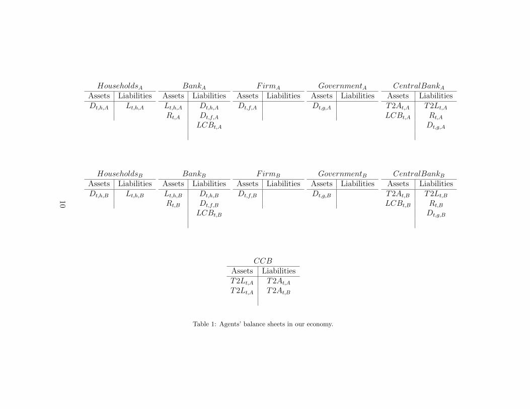
Figure 1 provides a graphical representation of all the transaction flowsin our economy, as described by the sequence reported above, while Table 1represents the balance sheets for each typology of agent, with the followingstock variables for each country c: household deposits (Dt,h,c), loans (Lt,h,c),government deposits (Dt,g,c), reserves (Rt,c), firm deposits (Dt,f,c), centralbank loans (LCBt,c), Target 2 claims for the national central bank (T2At,c),Target 2 liabilities for the national central bank (T2Lt,c). The model could

8

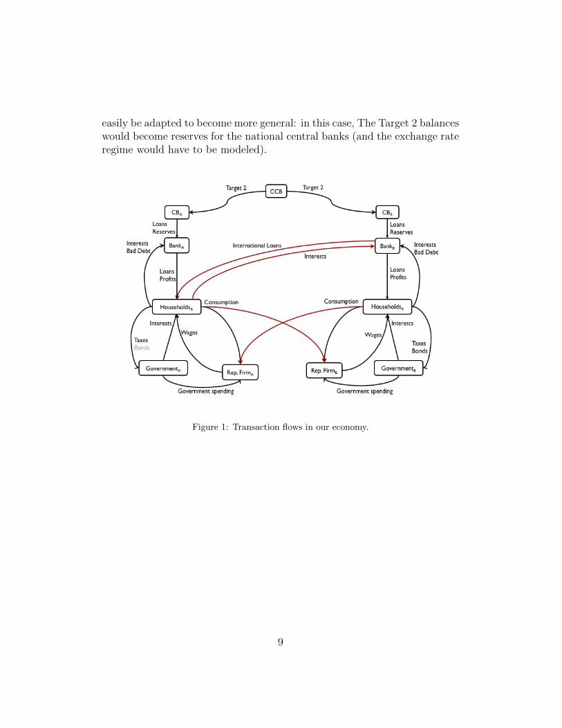
easily be adapted to become more general: in this case, The Target 2 balanceswould become reserves for the national central banks (and the exchange rateregime would have to be modeled).

Figure 1: Transaction flows in our economy.

9

HouseholdsAAssets LiabilitiesDt,h,A Lt,h,A

BankAAssets LiabilitiesLt,h,A Dt,h,A

Rt,A Dt,f,A

LCBt,A

FirmA

Assets LiabilitiesDt,f,A

GovernmentAAssets LiabilitiesDt,g,A

CentralBankAAssets LiabilitiesT2At,A T2Lt,A

LCBt,A Rt,A

Dt,g,A

HouseholdsBAssets LiabilitiesDt,h,B Lt,h,B

BankBAssets LiabilitiesLt,h,B Dt,h,B

Rt,B Dt,f,B

LCBt,B

FirmB

Assets LiabilitiesDt,f,B

GovernmentBAssets LiabilitiesDt,g,B

CentralBankBAssets LiabilitiesT2At,B T2Lt,B

LCBt,B Rt,B

Dt,g,B

CCBAssets LiabilitiesT2Lt,A T2At,A

T2Lt,A T2At,B

Table 1: Agents’ balance sheets in our economy.

10

2.1. Households

Household disposable income is the sum of wages (wt,h,c) and profits fromthe commercial bank of the country (πt,h,c), net of taxes (Tt,h,c).

ydt,h,c = wt,h,c + πt,h,c − Tt,h,c (1)

Wages are distributed by the firm at the beginning of each period t. Inparticular, the firm allocates the entire amount of revenues (Dt−1,F ) to allhouseholds based on constant individual income shares that are drawn from aPareto distribution (see Figure 2 in Section 3). Additionally, we assume thatthe bank distributes a fixed share (δ) of its profits (if any) to the householdsector based on the same exogenous individual income shares.

Consumption behaviour in our model is based on peer effects and imi-tation, in line with the empirical literature on behavioural economics show-ing that households tend to learn consumption patterns from their socialreference group, thereby comparing their living standard with that of theirneighbours or richer households (Cardaci, 2016; Fazzari and Cynamon, 2013).Our formulation is very similar to the Expenditure Cascades hypothesis in-troduced by Frank et al. (2014) and relies on upward-looking comparisons.

Cdt,h,c = k ydt,h,c + acCt−1,j,c (2)

ac = a− ap (3)

Equation 2 describes h’s desired consumption as a function of her dispos-able income (ydt,h) and the actual previous-period consumption of j, who isthe household ranking just above h in the income scale (i.e. j = h+ 1, basedon ascending disposable income ranking). k is the propensity to consume outof disposable income and it is unrelated to income level or rank (Frank et al.,2014), while ac is the country-specific effective rate of imitation, that is asensitivity measure such that 0 ≤ ac ≤ 1. When ac = 1, the impact of j onh’s consumption is maximum; whereas when ac = 0, there is no expenditurecascade. Equation 3 shows the calculation of the imitation sensitivity. Thisfollows the approach introduced by Belabed et al. (2013): we assume thatall individuals are associated with a “natural rate of imitation”, a, which isgrounded in the the quest for social status and upward-looking comparisonsand it is unrelated to country-specific factors. However, the effective rate

11

of imitation, ac, is computed by subtracting a penalty rate, ap, from thenatural rate. As argued by Belabed et al. (2013), the penalty rate reflectscountry-specific elements – such as the provision of public goods, the level ofsocial protection expenditure relative to GDP, the amount of public spendingin health, and so on – which lower the extent to which households seek toemulate their richer peers.

Eventually, households assess their own financial position: positive sav-ings take the form of zero interest rate deposits held at the commercial bankof the same country. On the contrary, if the sum of desired consumptionand the repayment on home and foreign loans from the previous period(RSc

t−1,h,c +RS−ct−1,h,c) is greater than the sum of disposable income and past

deposits, households have a positive demand for loans (Ldt,h).4

Ldt,h,c = max{0, Cd

t,h,c +RSt−1,h,c +RS−ct−1,h,c − ydt,h,c −Dt−1,h,c} (4)

Notice that borrowers in A are assumed to have a home bias, such thatthey first apply for a loan to the banking sector in their country. Hence, onlyin case of rationing in the domestic credit market, they will send their loanapplications abroad to the commercial bank in B.

Additionally, the actual individual demand for consumption is defined asthe minimum between desired consumption and household deposits, that ismin(Cd

t,h,c, Dt,h,c). Indeed, if h is credit-rationed she is not able to financeher desired consumption in full. In this case, demand for consumption isconstrained by the amount of household deposit.

Eventually households allocate individual demand at home and abroad(DCc

t,h,c and DC−ct,h,c respectively), based on the ratio between domestic andforeign prices (Pt,c/Pt,−c) multiplied by a sensitivity parameter (γ) (Equa-tions 5 and 6).5

DCct,h,c =

(1− γ Pt,c

Pt,−c

)min(Cd

t,h,c, Dt,h,c) (5)

DC−ct,h,c =

(γPt,c

Pt,−c

)min(Cd

t,h,c, Dt,h,c) (6)

4The repayment schedule on both home and foreign loans is defined in section 2.4.5Notice that γ is a positive parameter such that 1− γ Pt,c

Pt,−c≥ 0 and γ

Pt,c

Pt,−c≥ 0, that is

individual demand (at home or abroad) cannot be negative.

12

2.2. FirmsIn order to keep the structure of the model as simple as possible, we have

introduced a rather simplified aggregate productive sector in each country,with a representative firm owned by the domestic population. Each firmdistributes wages to the household sector based upon the already mentionedindividual Pareto shares.

The two firms also set total production (Qt,c) and prices (Pt,c) by react-ing to disequilibria in the goods market, as described by Equations 7 and 8.That is, Qt,c and Pt,c depend on their previous period level and on a sensi-tivity parameter (φQ,c and φP,c respectively) multiplied by the demand gap(gapt−1,c).

Qt,c = Qt−1,c (1 + φQ,c · gapt−1,c) (7)

Pt,c = Pt−1,c (1 + φP,c · gapt−1,c) (8)

The demand gap measures the real term excess demand or supply and it isdefined as the difference between aggregate demand (ADt,c) and production,divided by production itself (Equation 9).

gapt,c =ADt,c −Qt,c

Qt,c

(9)

Finally, aggregate demand (Equation 10) is the sum of private desiredconsumption, government spending (Gd

t,c, defined in the next section) andexports, which are computed as the sum of individual demand for goods byforeign households.

ADt,c =∑h∈c

DCct,h,c +Gd

t,c +∑h∈−c

DCct,h,−c (10)

2.3. GovernmentThe government in each country sets the ratio of desired public spend-

ing over GDP at the beginning of each period, based on a counter-cyclical

rule. In particular, the initial value of the ratio(

Gd

GDP

)changes based on its

sensitivity (φG) to the demand gap in the previous period.

Gdt,c

GDPt−1,c=

(Gd

c

GDPc

− φG gapt−1,c

)(11)

13

2.4. Banks

On the demand side, the credit market features households who apply fora loan in order to finance their desired consumption or to pay back the loanfrom the previous period. Additionally, some borrowers in financial distresscan do both.

The formation of credit supply follows the mechanism described in Car-daci and Saraceno (2016): the commercial bank sets the maximum allow-able credit supply (LSt,c) as the minimum between a multiple of its equity(NWBt,c) and a fraction (vt,c) of total credit demand (LDt,c).

LSt,c = min

[NWBt,c

β; vt,c LDt,c

](12)

A few remarks are necessary. First of all, notice that β identifies thecapital requirement coefficient so that, in line with the regulatory frameworkintroduced by Basel III (Basel Committee on Banking Supervision, 2011),the commercial bank has to comply with a prudential regulation.

Secondly, as already mentioned, bank B is allowed to lend internationally,so that the total credit demand (i.e. the sum of individual demand for loansby households) in B is equal to LDt,B =

∑h∈A L

dt,h,A +

∑h∈B L

dt,h,B, while

LDt,A =∑

h∈A Ldt,h,A.

Finally, also note that vt,c ∈ [vmin, vmax]. That is, each commercial bankendogenously changes the value of vt,c within two boundaries (vmin and vmax)that are exogenously set in the initialisation phase of the model (Conditions13 and 14). In particular, vt,c, which can be interpreted as the willingnessto lend of the banking system, evolves as a function of systemic risk whichis proxied by the household debt-to-GDP ratio (Xt,c) in the previous period.The evolution depends on a sensitivity threshold (χ), so that if the ratio ishigher (lower) than the threshold, the commercial bank decreases (increases)vt,c.

vt,c =

{vt−1,c + φv(vmin − vt−1,c) if Xt,c > χ (13)

vt−1,c + φv(vmax − vt−1,c) if Xt,c ≤ χ (14)

Notice that the two commercial banks are assumed to have the samesensitivity to system risk. However, while the bank in A is sensitive only tothe household debt in A, the bank in B focuses on the mean of the debt ratio

14

in the two countries, as its credit supply targets households of both A andB.

The bank in each country ranks households in ascending order basedon a measure of their financial soundness – namely the total debt serviceratio (TDS), defined as the ratio between household repayment scheduleand disposable income – and supplies credit by matching each individualdemand until it exhausts its credit supply. As already mentioned, householdsin A apply for a loan to the commercial bank of the same country. Oncecredit availability falls down to zero, households eventually send their loanapplications to the foreign bank in B. This circumstance takes place whenevervt,A < 1: in this case less financially sound applicants, that is households witha higher TDS, will be rationed on the domestic credit market. As a result,they apply for a loan at the commercial bank in B. If vt,B < 1, householdswill be credit rationed also in B and, as a consequence, they will not beable to pay back their previous loan and, in some cases, finance their desiredconsumption entirely. Therefore, they will go bankrupt, thus being excludedfrom the credit market for a limited number of periods (identified by theparameter freeze.).

We assume each loan is a one-period debt contract corresponding to arepayment schedule defined as RSt,h,c = Lt,h,c(1 + rLt,h,c), to be paid backentirely in the following period. In line with Cardaci (2016), Cardaci andSaraceno (2016) and Russo et al. (2016), the interest rate on loans is madeof three components (Equation 15).

rLt,h,c = rt + r̂t,c + rt,h,c (15)

r̂t is a system-specific component that reflects the sensitivity (ρ) of thebank to systemic risk (i.e. the household debt-to-GDP ratio) of the economy,

so that r̂t,A = ρdebtt−1,A

GDPt−1,Aand r̂t,B = ρ debtt−1

GDPt−1. Eventually, rt,h,c is a household-

specific component equal to µTDSt,h,c, where µ is the bank sensitivity tothe household total debt service ratio. Finally, rt is the policy rate set bythe supranational central bank at the beginning of each period as a reaction(φCB) to changes in the average demand gap of the economy (gapt−1,AB).6

6Notice that as we focus on demand fluctuations, quantities and prices move in thesame direction, so that the supranational central bank is implicitly targeting inflation aswell.

15

rt = rt−1 + φCB gapt−1,AB (16)

After completing all the transactions in the credit market, all borrowerswho have rolled over their debt can now pay back their outstanding loanfrom the previous period, RSt−1,h,c.

Also notice that, in case of negative net worth, each commercial bank isbailed out by the national central bank of the corresponding country via atransfer of assets.7

3. Model Results

We investigate the micro and macro properties of the model by means ofcomputer simulations. To this purpose we analyse three main scenarios anda set of policy experiments. In particular we replicate the following:

• Baseline scenario (BS): individual income shares remain constant throughthe simulations;

• Rising-inequality scenario (RS): income shares exogenously change overtime in both countries in order to simulate increasing income dispari-ties;

• Credit-inequality scenario (CS): the maximum propensity to lend ofthe banking sector increases in both countries together with the rise ofinequality as in RS.

The policy experiments include fiscal policies that are simulated with andwithout coordination between the two countries. In particular we replicate:

• a Keynesian policy consisting in a bolder reaction of desired govern-ment spending to the demand gap in RS;

7Note that central banks usually lend secured to commercial banks, thereby takingcollateral to protect against the possibility of loss due to credit and market risk (Rule,2015). However, as in Cardaci and Saraceno (2016), our simplified framework implies thatbailout operations do not require any collateral or reimbursement so that the nationalcentral bank does not receive any asset in exchange for the transfer of reserves to thecommercial bank. This simplification allows us to rule out banking crises in our model,and to focus exclusively on household debt as the trigger of financial instability.

16

• a Progressive policy implemented through changes in the marginal taxrates towards a more progressive tax system in RS and CS.

Additionally, we test the ability of the model to replicate some key microand macro empirical regularities by looking at cross-correlations and otherrelevant statistics.8 In doing so, we also exploit one of the main advantages ofthe agent-based approach, which consists in the analysis of the distributionof key economic variables among heterogeneous agents. This is particularlyuseful in order to shed some light on the microeconomic dynamics behindchanges in the aggregate patterns. Finally, we perform both univariate andmultivariate sensitivity analysis thus testing the robustness of model resultsto changes in parameter values.

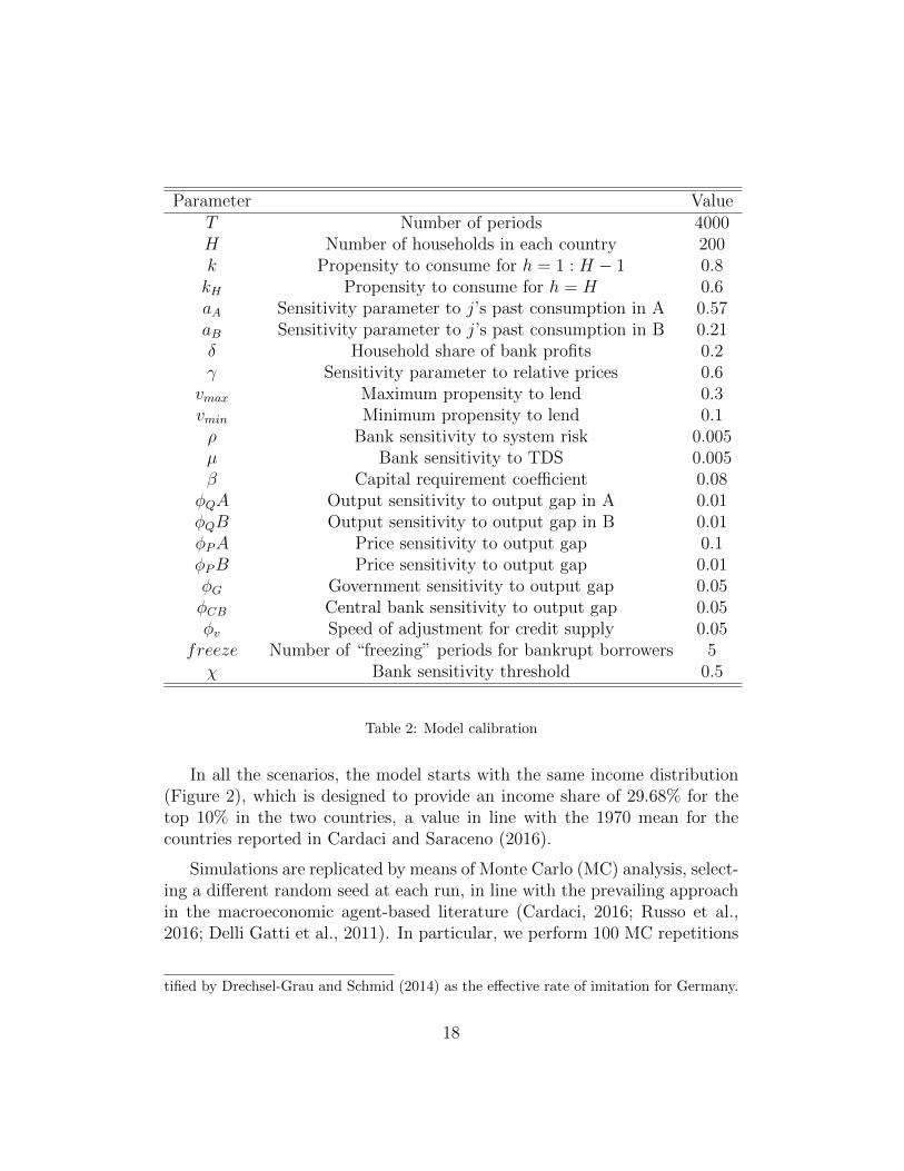
The model is calibrated as reported in Table 2. When possible, parametervalues are the same as in Cardaci and Saraceno (2016) or they are retrievedfrom the literature, such as for the value of the capital requirement coeffi-cient that is in line with Basel Committee on Banking Supervision (2011).Exceptions include aA and aB: the calculation of these two values followsa procedure similar to the one adopted by Belabed et al. (2013). First, foreach country we build a vector whose elements correspond to some key vari-ables that identify the importance of socio-economic factors (such as the longterm unemployment rate, the employment by job tenure interval, health ex-penditure as a percentage of GDP, etc.) that mitigate the impact of socialnorms, in line with approach discussed in Section 2.1. We collect the data foreach variable from different datasets with reference to Germany and Greece,which are used as proxies for the core and the periphery of the Eurozonerespectively. Eventually, we compute the Euclidean norm of the two vectorsto calculate the penalty rate for each of the two countries. These are equal to0.64 for Germany (i.e. country B) and 0.28 for Greece (country A). Finally,the effective rate of imitation is obtained by subtracting such penalty ratesfrom the natural rate, which is equal to 0.85.9 Hence, the effective rate ofimitation equals 0.21 for B (Germany) and 0.57 for A (Greece).10

8Notice that our modelling framework does not include many real world features, suchas investment in capital goods, employment dynamics in the labour market, innovationand progress. As such, we do not carry out a full-scale empirical validation. Rather, weinvestigate whether our simple framework captures some essential facts about inequalityand credit.

9The value of the natural rate of imitation is taken from Belabed et al. (2013).10Notice that the penalty rate for B falls within the range [0.18−0.35] empirically iden-

17

Parameter ValueT Number of periods 4000H Number of households in each country 200k Propensity to consume for h = 1 : H − 1 0.8kH Propensity to consume for h = H 0.6aA Sensitivity parameter to j’s past consumption in A 0.57aB Sensitivity parameter to j’s past consumption in B 0.21δ Household share of bank profits 0.2γ Sensitivity parameter to relative prices 0.6

vmax Maximum propensity to lend 0.3vmin Minimum propensity to lend 0.1ρ Bank sensitivity to system risk 0.005µ Bank sensitivity to TDS 0.005β Capital requirement coefficient 0.08

φQA Output sensitivity to output gap in A 0.01φQB Output sensitivity to output gap in B 0.01φPA Price sensitivity to output gap 0.1φPB Price sensitivity to output gap 0.01φG Government sensitivity to output gap 0.05φCB Central bank sensitivity to output gap 0.05φv Speed of adjustment for credit supply 0.05

freeze Number of “freezing” periods for bankrupt borrowers 5χ Bank sensitivity threshold 0.5

Table 2: Model calibration

In all the scenarios, the model starts with the same income distribution(Figure 2), which is designed to provide an income share of 29.68% for thetop 10% in the two countries, a value in line with the 1970 mean for thecountries reported in Cardaci and Saraceno (2016).

Simulations are replicated by means of Monte Carlo (MC) analysis, select-ing a different random seed at each run, in line with the prevailing approachin the macroeconomic agent-based literature (Cardaci, 2016; Russo et al.,2016; Delli Gatti et al., 2011). In particular, we perform 100 MC repetitions

tified by Drechsel-Grau and Schmid (2014) as the effective rate of imitation for Germany.

18

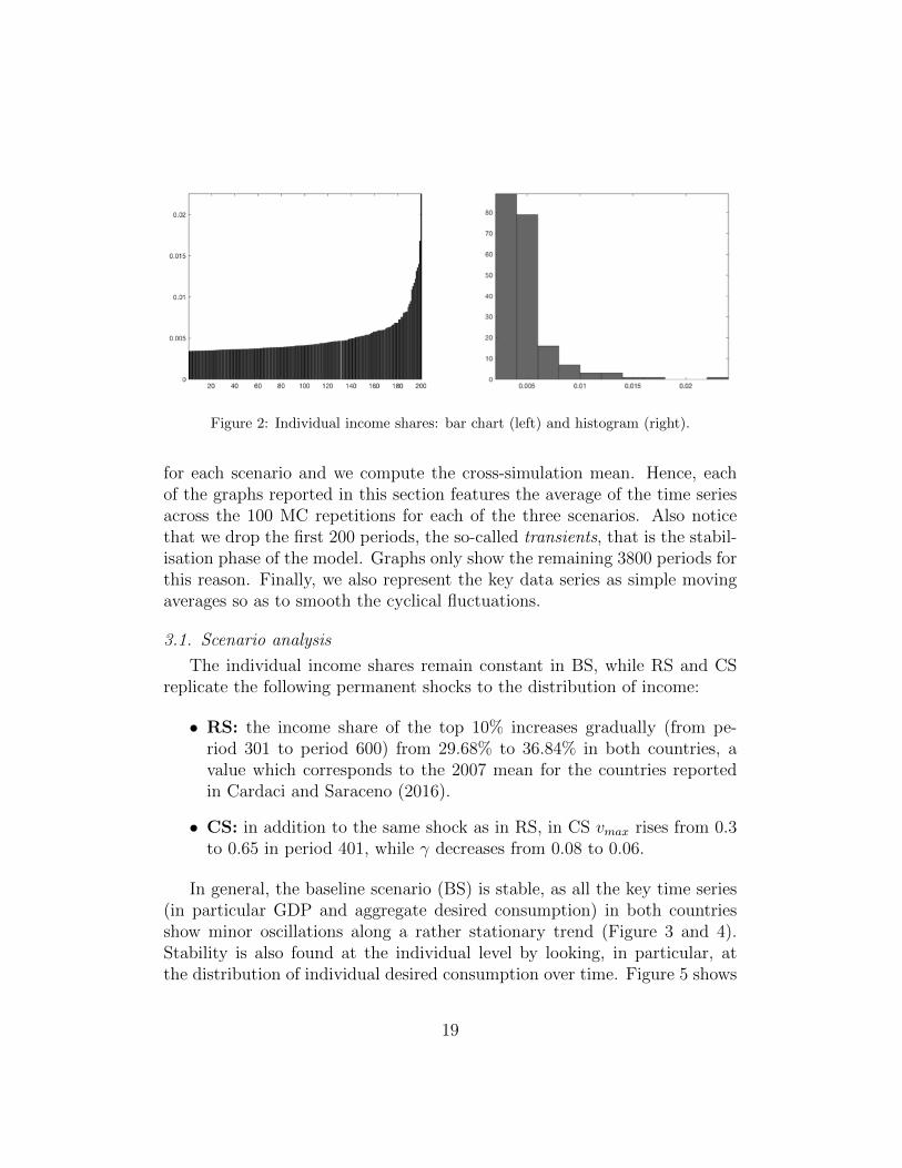
Figure 2: Individual income shares: bar chart (left) and histogram (right).

for each scenario and we compute the cross-simulation mean. Hence, eachof the graphs reported in this section features the average of the time seriesacross the 100 MC repetitions for each of the three scenarios. Also noticethat we drop the first 200 periods, the so-called transients, that is the stabil-isation phase of the model. Graphs only show the remaining 3800 periods forthis reason. Finally, we also represent the key data series as simple movingaverages so as to smooth the cyclical fluctuations.

3.1. Scenario analysis

The individual income shares remain constant in BS, while RS and CSreplicate the following permanent shocks to the distribution of income:

• RS: the income share of the top 10% increases gradually (from pe-riod 301 to period 600) from 29.68% to 36.84% in both countries, avalue which corresponds to the 2007 mean for the countries reportedin Cardaci and Saraceno (2016).

• CS: in addition to the same shock as in RS, in CS vmax rises from 0.3to 0.65 in period 401, while γ decreases from 0.08 to 0.06.

In general, the baseline scenario (BS) is stable, as all the key time series(in particular GDP and aggregate desired consumption) in both countriesshow minor oscillations along a rather stationary trend (Figure 3 and 4).Stability is also found at the individual level by looking, in particular, atthe distribution of individual desired consumption over time. Figure 5 shows

19

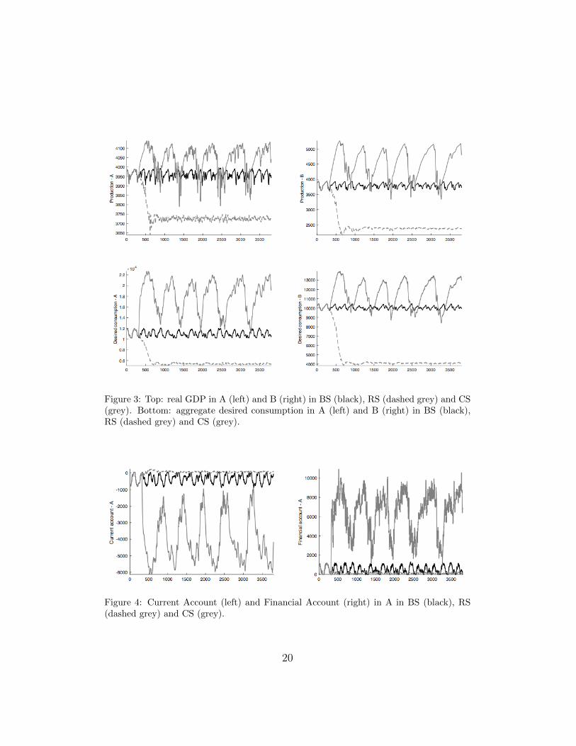
Figure 3: Top: real GDP in A (left) and B (right) in BS (black), RS (dashed grey) and CS(grey). Bottom: aggregate desired consumption in A (left) and B (right) in BS (black),RS (dashed grey) and CS (grey).

Figure 4: Current Account (left) and Financial Account (right) in A in BS (black), RS(dashed grey) and CS (grey).

20

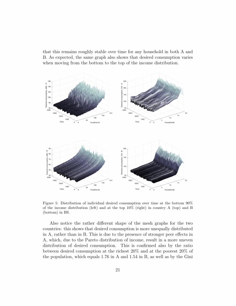
that this remains roughly stable over time for any household in both A andB. As expected, the same graph also shows that desired consumption varieswhen moving from the bottom to the top of the income distribution.

Figure 5: Distribution of individual desired consumption over time at the bottom 90%of the income distribution (left) and at the top 10% (right) in country A (top) and B(bottom) in BS.

Also notice the rather different shape of the mesh graphs for the twocountries: this shows that desired consumption is more unequally distributedin A, rather than in B. This is due to the presence of stronger peer effects inA, which, due to the Pareto distribution of income, result in a more unevendistribution of desired consumption. This is confirmed also by the ratiobetween desired consumption at the richest 20% and at the poorest 20% ofthe population, which equals 1.76 in A and 1.54 in B, as well as by the Gini

21

coefficient for desired consumption, which is equal (on average) to 0.13 in Aand 0.09 in B (Table 3).

Variable Scenario Average 20/20 ratio Average Gini coefficientA B A B

Individual consumptionBS 2.03 1.53 0.25 0.09RS 4.57 3.29 0.39 0.27CS 5.84 3.38 0.41 0.29

Individual desired consumptionBS 1.76 1.54 0.13 0.09RS 3.95 3.35 0.31 0.27CS 4.71 3.48 0.35 0.29

Desired consumption ratioBS 1.14 0.99 0.09 0.08RS 1.21 1.01 0.12 0.09CS 1.33 1.11 0.15 0.11

Table 3: Different measures of (actual and desired) consumption inequality in A and B inthe three scenarios.

Eventually, when inequality rises but credit conditions are unchanged,the economy performs rather badly in both A and B compared to the base-line: production falls and it remains persistently below its baseline level. Thedynamics of the balance of payments shows a minor increase in the currentaccount of A. On the contrary, the rise of inequality in CS results in a muchlarger current account deficit for A. Moreover, the time series of GDP showthe presence of major boom-and-bust dynamics in both economies, with big-ger magnitude in B, as confirmed by Table 4.

Let us now provide a detailed discussion on the impact of growing incomeinequality with and without changes in the level of financial deepening in theeconomy.

RS scenario

The impact of rising inequality on the economy of the two countries isroughly similar, in that higher income disparities with unchanged credit con-ditions eventually lead to falling GDP and aggregate desired consumption(Figure 3). The negative performance of the two countries is explained bythe increase of income disparities in the presence of peer effects without anyincrease in the willingness to lend of the banking sector or any change in thecapital requirement coefficient. Indeed, desired consumption rises for a fewperiods after the inequality shock as a consequence of growing expenditure

22

Variable Scenario Mean Coefficient of variationA B A B

GDPBS 3961.20 3789.65 0.0045 0.0194RS 3737.21 2445.47 0.0125 0.1131CS 4038.20 4535.30 0.0178 0.1037

Aggregate desired consumptionBS 10994.84 10050.56 0.0473 0.0173RS 5715.05 4451.63 0.1892 0.2737CS 18051.39 11571.48 0.1616 0.1187

Household debtBS 1576.97 960.11 0.2242 0.3878RS 681.078 680.93 0.2063 0.2282CS 13873.14 3832.38 0.3280 0.6714

Current accountBS -332.42 332.42 -0.7659 0.7659RS 65.06 -65.06 0.8416 -0.8416CS -4008.95 4008.95 -0.3491 0.3491

Domestic consumption (% of GDP)BS 23.77 21.38 0.0210 0.0053RS 26.60 17.63 0.0310 0.0505CS 28.53 17.51 0.0414 0.0277

Exports (% of GDP)BS 32.34 35.24 0.0138 0.0259RS 29.58 28.59 0.0252 0.0293CS 27.71 20.20 0.0426 0.0586

Table 4: Key statistics for selected variables in the three scenarios.

cascades in both economies, even though the imitation effect is larger in A.This is consistent with the empirical evidence by Bertrand and Morse (2016),who show that systematic changes in the behaviour of the non-rich individ-uals that result in greater spending, after an increase of top income levels,can be linked to social comparison. However, since the level of financialdeepening has not been modified, households at the bottom of the incomedistribution do not find the necessary resources to finance their higher de-sired consumption so that greater inequality eventually triggers the fall inconsumption and GDP in both economies. This result is also in line withthe closed economy version of this model (Cardaci and Saraceno, 2016).

It is interesting to analyse the distribution of desired consumption follow-ing the increase in inequality, also in this scenario. This allows in fact to havea better understanding of the mechanisms driving model dynamics. Figure 6shows that this variable is, on average, much higher for households at the topof the income distribution, while it is lower for those at the bottom. Table3 shows that both the average 20/20 ratio and the Gini coefficient increasein RS compared to BS in both A and B, thus indicating that rising incomeinequality also results in greater consumption inequality. Hence, our find-

23

Figure 6: Distribution of individual desired consumption over time at the bottom 90%of the income distribution (left) and at the top 10% (right) in country A (top) and B(bottom) in RS.

24

ing supports the recent empirical result that consumption inequality tracksincome inequality (Aguiar and Bils, 2015; Attanasio et al., 2014).

As in Cardaci (2016), it is possible to spotlight the economic pressure thatrising inequality under peer effects has on poorer households, by analysing thechange in the distribution of the desired consumption ratio, that is the ratiobetween individual desired consumption and income at the beginning of eachperiod. Our analysis shows that such measure increases for all households,even though it is slightly more unevenly distributed in RS compared to BS,as the corresponding average 20/20 ratio increases from 1.14 in BS to 1.21 inRS. Also the average Gini coefficient increases in RS compared to BS. Thissuggests that rising inequality in a poorly financialised context worsens theperformance of the economy as the increase in desired consumption by richerindividuals does not compensate for the fall by poorer households. As such,the economy enters a recession in both countries.

As already mentioned, the recession in RS is accompanied by a minorincrease in the current account of A (Figure 4), which is the consequenceof a reduction in imports (-29.57% in absolute real terms) that exceeds thereduction in exports (-13.69% in absolute real terms). Indeed, since the rela-tive price of goods in A with respect to B falls from 0.98 to 0.85, householdsin A increase the share of demand for goods allocated at home.

CS scenario

In this scenario, higher income inequality under peer effects and a greaterlevel of financialisation lead to an increase in desired consumption in bothcountries (Figure 3). Households in country A, who have stronger imitationin consumption, borrow extensively from the foreign banking sector in orderto finance consumption of both domestic and foreign goods. The consequenceis the emergence of a current account deficit and a financial account surplusfor A, with symmetrically different dynamics for B (Figure 4). Eventually,the massive accumulation of household debt implies a greater number ofhousehold defaults and an increase in the perception of risk by the foreignbanking sector, which lowers the credit supply thus contributing to a contrac-tion of consumption spending. Hence, the economies experience a financialaccount reversal and a recession. Therefore, this scenario is characterised bythe presence of endogenous business cycle fluctuations along a constant trend(Figure 3).

Our results seem to go against the stream of literature that was prevailingin the period before the financial crisis in the United States, which welcomed

25

the greater and easier access to credit as an efficient means to insure againstincome fluctuations (Krueger and Perri, 2006). Indeed, in our model, higheravailability of credit in a context of rising inequality comes at the price ofgreater instability in the overall economy and the emergence of external im-balances between the two countries.

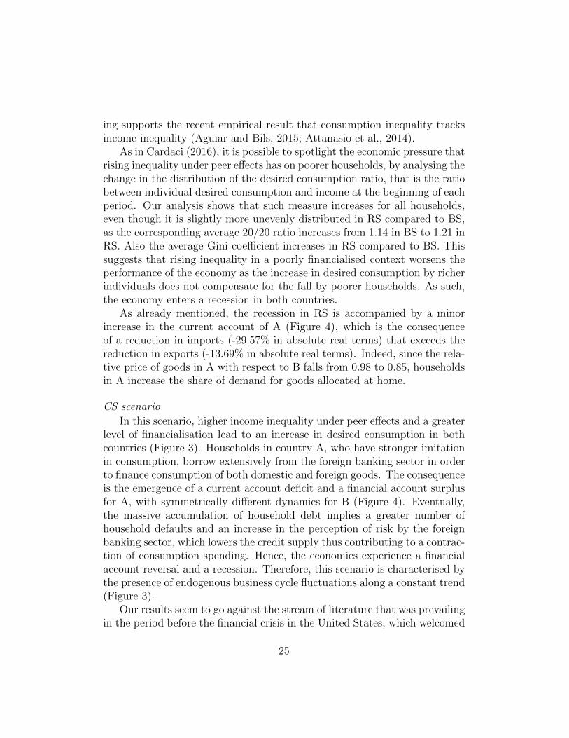
Figure 7: Distribution of individual desired consumption over time at the bottom 90%of the income distribution (left) and at the top 10% (right) in country A (top) and B(bottom) in CS.

Let us provide a detailed analysis of the three major phases of each busi-ness cycle, corresponding to the expansion of the economy, the turning pointand, in the end, the recession.

Economic expansion. Growing income disparities impact on desired con-sumption which rises dramatically in both countries (Figure 3). Also in CS,

26

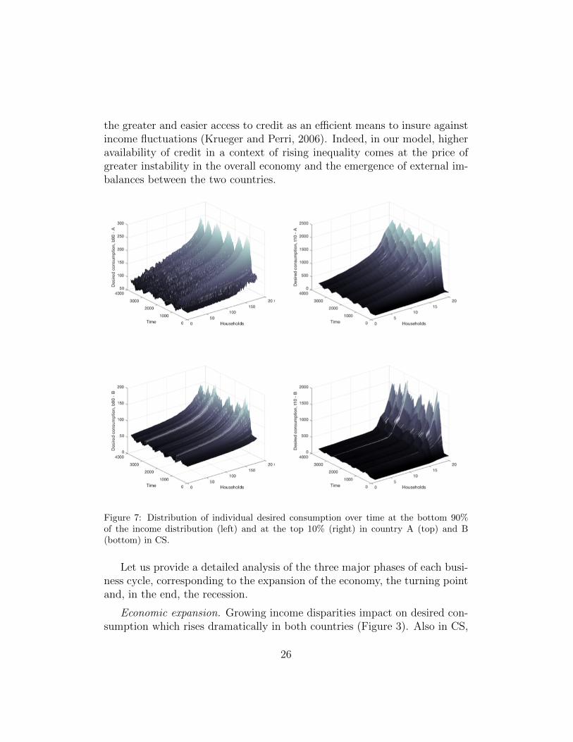
it is possible to evaluate the distribution of desired consumption at the indi-vidual level (Figure 7). Table 3 shows that both the average 20/20 ratio andthe average Gini coefficient for actual and desired consumption are larger inCS, in country A and in B. Such measures of inequality increase also for thedesired consumption ratio in both countries. As in the previous scenario, andsimilar to Cardaci (2016), this finding suggests that households at the bot-tom of the income distribution experience a greater need for loans to financegreater desired consumption in order to catch-up with households who rankabove them in the income scale. Indeed, Figure 8 shows that aggregate de-sired consumption is positively correlated with aggregate consumption loansin both A and B (particularly at lag 0, 1 and 2). Hence, rising inequalityresults in greater expenditure cascades that trigger higher credit demand inthe present and in future periods.

Figure 8: Cross-correlation between aggregate desired consumption and demand for con-sumption loans in A (left) and B (right) in CS.

Notice that, in the initial phase, credit demand rises only in A (Figure 9)due to stronger peer effects in consumption compared to country B. Hence,a greater number of people at the bottom of the distribution in country Aneed external finance to pay for the increased desired consumption.

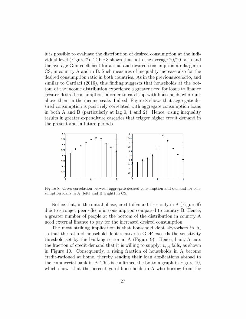
The most striking implication is that household debt skyrockets in A,so that the ratio of household debt relative to GDP exceeds the sensitivitythreshold set by the banking sector in A (Figure 9). Hence, bank A cutsthe fraction of credit demand that it is willing to supply: vt,A falls, as shownin Figure 10. Consequently, a rising fraction of households in A becomecredit-rationed at home, thereby sending their loan applications abroad tothe commercial bank in B. This is confirmed the bottom graph in Figure 10,which shows that the percentage of households in A who borrow from the

27

Figure 9: Top: total credit demand in CS (black) compared to BS (grey) in country A(left) and B (right); bottom: household debt relative to GDP in CS (black) compared toBS (grey) in country A (left) and B (right).

bank in B rises from roughly 20% to almost 80% in the aftermath of theshock. In fact, the two series – namely the willingness to lend of the bankingsector in B and the percentage of households in A who borrow from the bankabroad – are strictly correlated (77.1%, significant at 5%).11

Notice that even though household debt in A keeps on rising, the bankingsector in B is still willing to provide an increasing fraction of credit (middlegraph in Figure 10). The reason why vt,B does not fall following a riseof household debt in A is that the commercial bank in B sets its sensitivitythreshold based on the average value of household debt to GDP in the overalleconomy (as pointed out in Section 2.4). That is, since households in B are

11In general, it seems that the capital requirement coefficient plays a very limited rolein driving model dynamics in CS. In fact, most of the times (98.76% of all periods t, onaverage across simulations) the maximum bank supply is equal to the fraction vt,c of totalcredit demand that the bank in each country is willing to supply (see Equation 12 above).

28

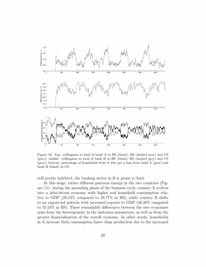
Figure 10: Top: willingness to lend of bank A in BS (black), RS (dashed grey) and CS(grey); middle: willingness to lend of bank B in BS (black), RS (dashed grey) and CS(grey); bottom: percentage of households from A who get a loan from bank A (grey) andbank B (black) in CS.

still poorly indebted, the banking sector in B is prone to lend.At this stage, rather different patterns emerge in the two countries (Fig-

ure 11): during the ascending phase of the business cycle, country A evolvesinto a debt-driven economy with higher real household consumption rela-tive to GDP (28.53% compared to 23.77% in BS), while country B shiftsto an export-led pattern with increased exports to GDP (40.20% comparedto 35.24% in BS). These remarkable differences between the two economiesarise from the heterogeneity in the imitation parameters, as well as from thegreater financialisation of the overall economy. In other words, householdsin A increase their consumption faster than production due to the increased

29

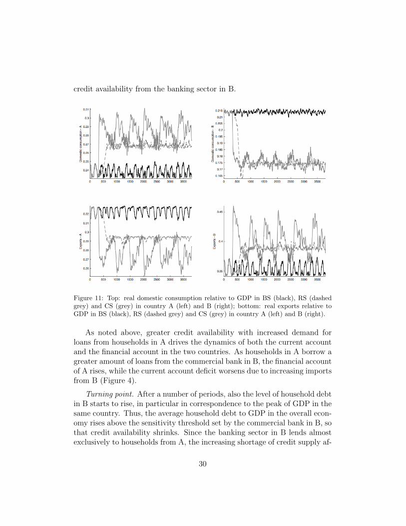
credit availability from the banking sector in B.

Figure 11: Top: real domestic consumption relative to GDP in BS (black), RS (dashedgrey) and CS (grey) in country A (left) and B (right); bottom: real exports relative toGDP in BS (black), RS (dashed grey) and CS (grey) in country A (left) and B (right).

As noted above, greater credit availability with increased demand forloans from households in A drives the dynamics of both the current accountand the financial account in the two countries. As households in A borrow agreater amount of loans from the commercial bank in B, the financial accountof A rises, while the current account deficit worsens due to increasing importsfrom B (Figure 4).

Turning point. After a number of periods, also the level of household debtin B starts to rise, in particular in correspondence to the peak of GDP in thesame country. Thus, the average household debt to GDP in the overall econ-omy rises above the sensitivity threshold set by the commercial bank in B, sothat credit availability shrinks. Since the banking sector in B lends almostexclusively to households from A, the increasing shortage of credit supply af-

30

fects mostly foreign households, thus having two major consequences: first,the percentage of successful credit applicants among households in A startsto fall – from almost 80% it eventually reaches roughly 20%) – so that house-hold debt in A decreases and the willingness to lend of the commercial bankof A improves; secondly, a growing percentage of households from A sendtheir loan applications back to the commercial bank in the same country.

Bust. The whole process of credit contraction generates a dramatic fallof aggregate demand in A, since households lack the external resources tofinance desired consumption. On the other hand, A’s imports drop and itscurrent account improves. The financial account of A, instead, falls as a resultof the lower amount of loans from the foreign banking system. Country Balso experiences a recession, but in this case it is characterised by plungingreal exports (equal to A’s imports).

Notice that all dynamics revert after a few periods, such that a newbusiness cycle starts again whenever the commercial bank in B restores itswillingness to lend.

3.2. Policy responses

In addition to the three scenarios discussed above, we analyse how modeldynamics change when policy makers react to rising inequality by imple-menting different kinds of fiscal policies in the two countries. In particular,first we assess the effectiveness of a Keynesian type of policy consisting in abolder reaction of desired government spending to the demand gap. Eventu-ally, we analyse the consequences of a change in the tax system into a moreprogressive one. Similar to the closed economy version of the model, also inthis case our results suggest that the second type of policy has a clearer andstronger effect on the overall economy with respect to an intervention of thefirst type.

The simulation procedure for the Keynesian policy follows Cardaci andSaraceno (2016), in that we randomly draw 20 different values for φG andfor each of them we also perform 100 MC repetitions in each of the threescenarios (hence, we perform 6000 computer simulations in total). This policyintervention is simulated with and without coordination: in the first case, φG

changes equally in both countries, whereas in the second case the change isdifferent in A and B.

Regardless of the presence of coordination, our results indicate that abolder fiscal policy does not prevent the economy from entering a recession

31

in both countries in RS, and its implications are also non-tangible in the CSscenario as the time series of all the key variables do not show any significantdifference in terms of magnitude, duration and volatility of the boom andbust cycles.

The second kind of fiscal policy consists in changing the marginal taxrates in a way such that the system becomes more progressive. In particular,we simulate 10 different compositions of the marginal tax rates (which arethe same in the countries) and we run 100 Monte Carlo repetitions for eachof them (thus having 1000 simulations in total).

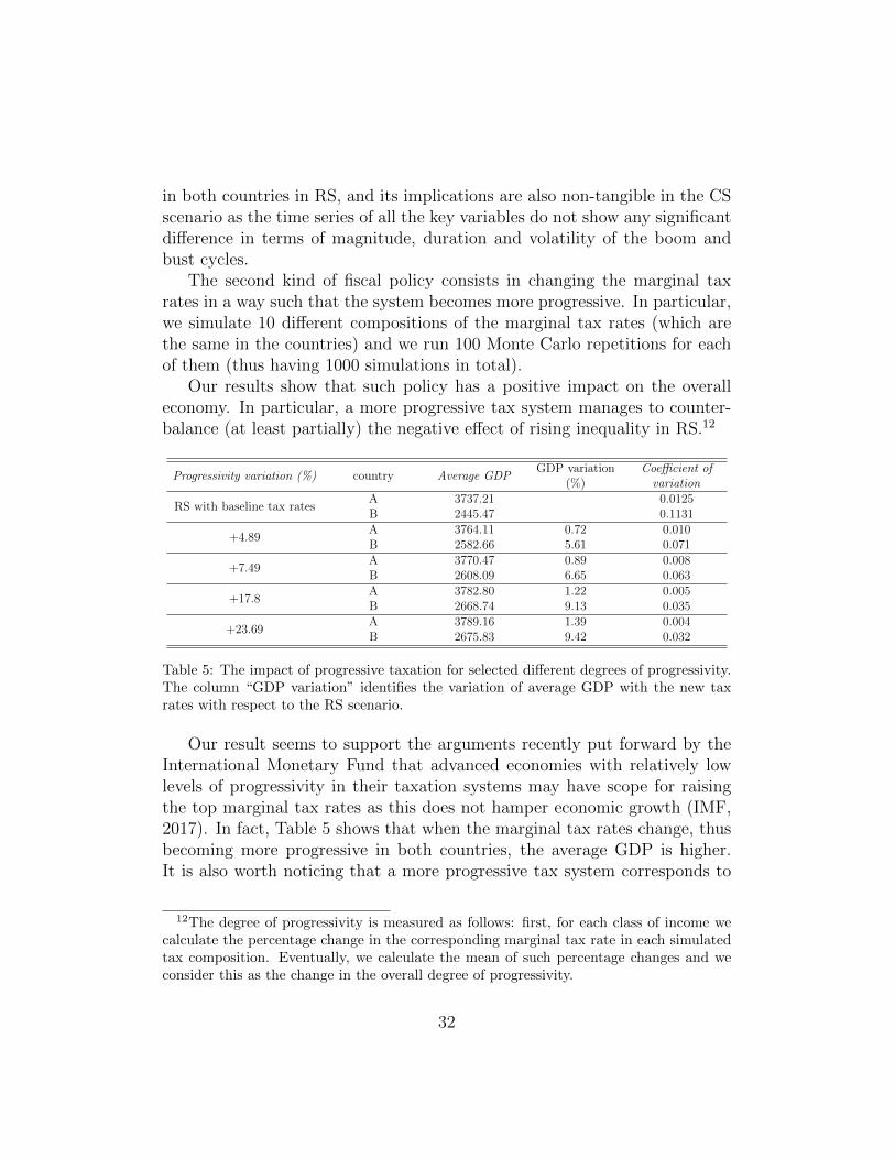
Our results show that such policy has a positive impact on the overalleconomy. In particular, a more progressive tax system manages to counter-balance (at least partially) the negative effect of rising inequality in RS.12

Progressivity variation (%) country Average GDPGDP variation

(%)Coefficient of

variation

RS with baseline tax ratesA 3737.21 0.0125B 2445.47 0.1131

+4.89A 3764.11 0.72 0.010B 2582.66 5.61 0.071

+7.49A 3770.47 0.89 0.008B 2608.09 6.65 0.063

+17.8A 3782.80 1.22 0.005B 2668.74 9.13 0.035

+23.69A 3789.16 1.39 0.004B 2675.83 9.42 0.032

Table 5: The impact of progressive taxation for selected different degrees of progressivity.The column “GDP variation” identifies the variation of average GDP with the new taxrates with respect to the RS scenario.

Our result seems to support the arguments recently put forward by theInternational Monetary Fund that advanced economies with relatively lowlevels of progressivity in their taxation systems may have scope for raisingthe top marginal tax rates as this does not hamper economic growth (IMF,2017). In fact, Table 5 shows that when the marginal tax rates change, thusbecoming more progressive in both countries, the average GDP is higher.It is also worth noticing that a more progressive tax system corresponds to

12The degree of progressivity is measured as follows: first, for each class of income wecalculate the percentage change in the corresponding marginal tax rate in each simulatedtax composition. Eventually, we calculate the mean of such percentage changes and weconsider this as the change in the overall degree of progressivity.

32

lower volatility, as the coefficient of variation is lower for higher progressivityvariations.

Hence, a more progressive tax system allows a greater share of poorerhouseholds to rely on internal financial resources, thus implying also lowerlevels of debt accumulation and a more stable economy. As such, our sim-ulations confirm the positive impact of a progressive tax system also in thecontext of an open economy (within a currency union). In a sense, redis-tributive policies bring the system back towards the baseline scenario withstable GDP dynamics. Notice, however, that GDP still remains below thebaseline value in both countries and this result holds true for any of the 10simulated tax systems.

To conclude this section, we want to point out that our rather simpli-fied modelling framework does not allow to take into account the possibledistortionary effects that greater progressivity may have on other aspects ofthe economy, such as the functioning of labour markets or firm profits andinvestment decisions. The interpretation of our results should therefore belimited to considering that an increase in progressivity is more efficient thanmacroeconomic policies at tackling the expenditure cascades that follow therise of inequality. Any further interpretation would be unwarranted giventhe simplified structure of our model.

3.3. Sensitivity Analysis

The purpose of univariate and multivariate sensitivity analysis is to assessthe robustness of our results by running the simulations under different cal-ibrations. In other words, we want to understand whether the main findingsof our model are biased by the choice of our parameter vector.

Univariate analysis allows to look at variations in the outcome of themodel while changing one parameter at a time, leaving all the other con-stant. Eventually, “the model is then believed to be good if the outputvalues of interest do not vary significantly despite significant changes in theinput values” (Delli Gatti et al., 2011, p. 77). Hence, we follow the same ap-proach adopted for the robustness check of the closed-economy version of thismodel reported in Cardaci and Saraceno (2016): we select 17 parameters andwe randomly draw 20 values within a reasonable min-max interval for eachindividual parameter at a time, leaving all the other ones unchanged. Foreach of the 20 parameter values, we run 100 Monte Carlo repetitions, eachwith a different random seed, in all the three scenarios (i.e. BS, RS and CS).As such, for each single parameter, the univariate analysis results in 6000

33

ParameterVariation in

parameter (%)Country

Variation inGDP-BS at t

500 (%)

Variation inGDP-RS at t

1000 (%)

Variation inGDP-CS at t

1000 (%)

k 45.89A 4.29 10.78 8.67B 29.36 111.95 75.13

aA 113.31A 4.12 9.31 6.22B 36.12 82.66 58.48

aB 154.14A 3.87 10.04 9.33B 28.01 87.98 90.93

ρ 3325.3A 0.89 2.29 3.54B 6.29 17.91 23.86

µ 3466.94A 1.48 4.10 3.35B 5.29 23.63 20.33

φQA 866.31A 14.31 20.11 18.47B 8.93 24.59 24.58

φQB 287.84A 1.12 7.08 2.79B 15.02 62.43 32.96

γ 227.46A 2.73 7.16 6.20B 7.62 32.07 28.19

δ 266.97A 2.23 5.51 5.43B 15.47 54.46 38.41

φPA 166.47A 1.41 4.39 5.53B 3.48 21.63 30.07

φPB 837.36A 2.18 10.15 3.43B 14.29 30.85 16.54

φG 737.71A 1.31 4.35 3.67B 5.43 26.06 18.67

φCB 838.14A 1.09 5.72 2.94B 6.34 32.69 17.75

φV 360.01A 1.08 6.02 3.19B 6.81 29.12 20.79

χ 471.85A 0.73 4.53 7.31B 8.24 26.97 71.63

freeze 596.13A 2.38 3.01 4.47B 22.21 35.21 27.44

β 341.75A 1.95 6.38 11.76B 3.41 4.64 9.89

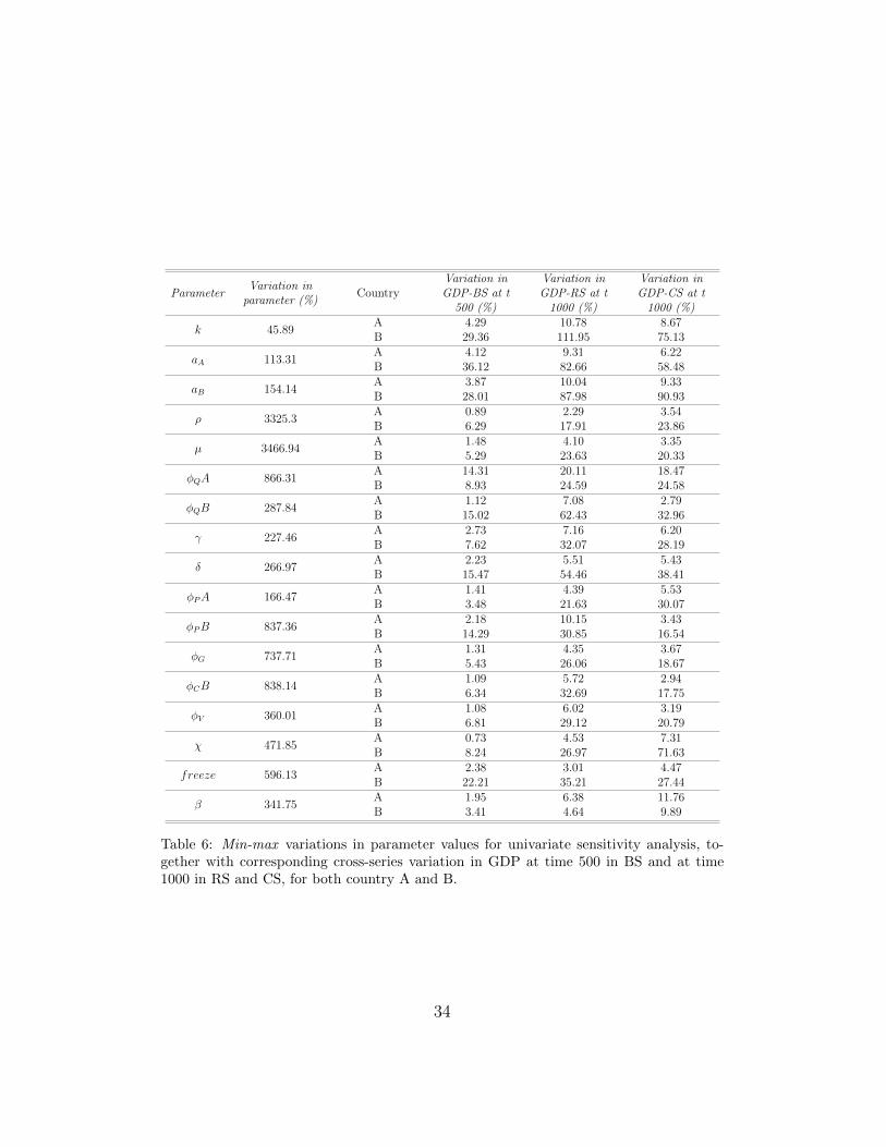
Table 6: Min-max variations in parameter values for univariate sensitivity analysis, to-gether with corresponding cross-series variation in GDP at time 500 in BS and at time1000 in RS and CS, for both country A and B.

34

simulations. Since we explore 17 parameters, we run 102000 simulations intotal.

The results of our univariate analysis highlight the robustness of our re-sults. In fact, in most cases, output variations are greatly smaller than thevariations in the parameters. Table 6 reports the variation for each parame-ter between its minimum and maximum value in the sensitivity analysis andthe corresponding cross-series variation in GDP at time 500 for BS and attime 1000 for RS and CS for both country A and B. Results also confirmthat country A is less sensitive to changes in model parameters comparedto country B since, for any change in the calibration of the model, min-maxvariations in model output are larger in country B (with the exception of theunivariate analysis of φQA in BS). Among the most relevant parameters, interms of impact on model dynamics, the univariate analysis seems to confirmthe primary role of the consumption parameters k, aA and aB. Comparedto the closed economy model (Cardaci and Saraceno, 2016), the min-maxcross-series variation in GDP is larger in RS than in CS in most cases, suchas for univariate changes of k, µ, γ, etc.

Another robustness check that we perform consists in computing the per-centage of consistent simulations for each of the parameters tested in theunivariate analysis. To this purpose, we calculate the mean and the varianceof selected key variables (i.e. GDP, desired consumption, household debt,credit demand and household default rate) along the entire time span in thethree scenarios for each of the two countries. Eventually, we compare thesevalues, obtained under the different calibrations used in the sensitivity anal-ysis, with the same values obtained with the standard calibration reportedin Table 2.

For example, based on the standard calibration, both the mean and thevariance of GDP are lower in RS and higher in CS, compared to the baselinevalues, in both A and B. As such, we check whether GDP has the samequalitative behaviour in terms of mean and variance in any other univariatesimulation. For instance, we find that, ceteris paribus, most of the randomlyselected values of k imply that both the mean and the variance of GDP arelower in RS and higher in CS. In particular, we claim that 80.83% of theunivariate simulations for k are successful.

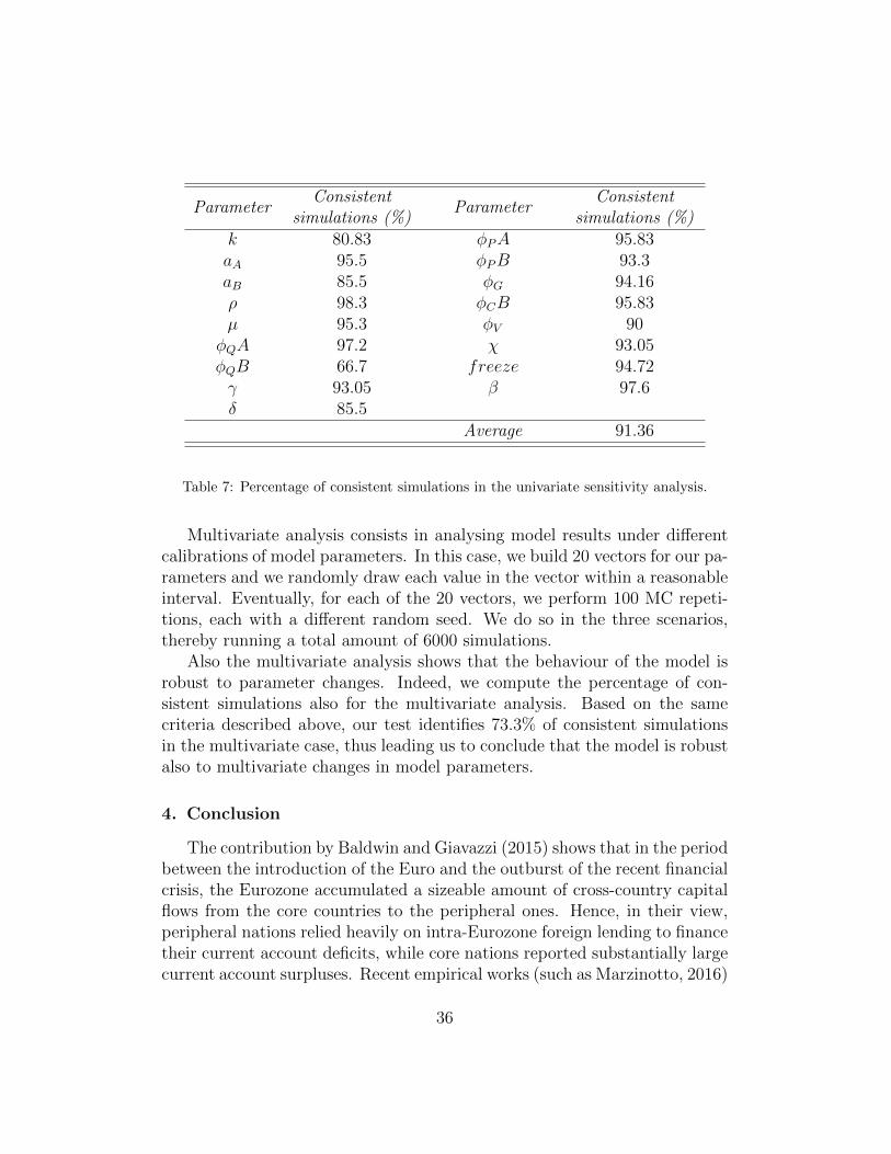
After repeating this experiment for all the parameters tested in the uni-variate analysis (Table 7), we find that, on average, 91.36% of univariatesimulations are consistent with our initial calibration, based on the criterionmentioned above.

35

ParameterConsistent

simulations (%)Parameter

Consistentsimulations (%)

k 80.83 φPA 95.83aA 95.5 φPB 93.3aB 85.5 φG 94.16ρ 98.3 φCB 95.83µ 95.3 φV 90

φQA 97.2 χ 93.05φQB 66.7 freeze 94.72γ 93.05 β 97.6δ 85.5

Average 91.36

Table 7: Percentage of consistent simulations in the univariate sensitivity analysis.

Multivariate analysis consists in analysing model results under differentcalibrations of model parameters. In this case, we build 20 vectors for our pa-rameters and we randomly draw each value in the vector within a reasonableinterval. Eventually, for each of the 20 vectors, we perform 100 MC repeti-tions, each with a different random seed. We do so in the three scenarios,thereby running a total amount of 6000 simulations.

Also the multivariate analysis shows that the behaviour of the model isrobust to parameter changes. Indeed, we compute the percentage of con-sistent simulations also for the multivariate analysis. Based on the samecriteria described above, our test identifies 73.3% of consistent simulationsin the multivariate case, thus leading us to conclude that the model is robustalso to multivariate changes in model parameters.

4. Conclusion

The contribution by Baldwin and Giavazzi (2015) shows that in the periodbetween the introduction of the Euro and the outburst of the recent financialcrisis, the Eurozone accumulated a sizeable amount of cross-country capitalflows from the core countries to the peripheral ones. Hence, in their view,peripheral nations relied heavily on intra-Eurozone foreign lending to financetheir current account deficits, while core nations reported substantially largecurrent account surpluses. Recent empirical works (such as Marzinotto, 2016)

36

show that such imbalances in the Eurozone seem to be due to the increase inincome disparities in a context of financial deepening. Indeed, easier accessto credit for the poorer segments of society resulted in a massive accumu-lation of household debt via domestic and foreign lending, thereby leadingto current account deficits in the periphery and surpluses in the core. Ingeneral, Belabed et al. (2013) and Kumhof et al. (2012) show that risinginequality can determine a diverging pattern in the balance of payments ofdifferent countries, depending on the level of financialisation of the economy.

In line with these contributions, our paper extends Cardaci and Saraceno(2016) by introducing two countries operating in a currency union. Ourmodel allows to capture the major role that inequality plays in determininglarge external imbalances, in line with Kumhof et al. (2012) and Belabedet al. (2013). In particular, our results suggest that rising inequality witha higher level of financial deepening leads to the emergence of a debt-ledconsumption growth regime in the country with stronger peer effects, whileresulting in an export-led regime and sluggish internal demand growth in theother country, as suggested by Stockhammer (2015). The former records acurrent account deficit and a financial account surplus due to the massiveinflow of consumption loans supplied by the foreign banking sector, whichallow households to finance the higher desired spending for consumption athome and abroad. Hence, our model captures the flow of capital that financesthe imbalances over the expanding phase of the economy. Eventually, acrisis emerges endogenously as a consequence of the massive accumulationof household debt that triggers a change in the perception of system risk onbehalf of the banking sector of the lending country. As such, a sudden stopoccurs, in that the representative commercial bank in this country shrinksthe credit supply thereby forcing households in the deficit country to lowertheir domestic consumption and imports substantially.

We believe that our model represents a suitable theoretical frameworkthat contributes to the study of these macroeconomic imbalances in the Eu-rozone in the presence of rising inequality. Yet, different improvements couldbe implemented in future research. In our view, the most interesting exten-sion might consist in the introduction of endogenous wage inequality, whichcould be implemented with the introduction of heterogeneous firms that canhire and fire workers, thus allowing for the simulation of bargain processesin wage setting mechanisms. This would also allow to study changes in un-employment dynamics in the different phases of the economic cycle.

37

Acknowledgement

We are particularly grateful to the participants at the 2016 ComplexityWorkshop at the University of Hamburg, the 2017 EUROFRAME confer-ence in Berlin, the Conference on “Finance and growth in the aftermath ofthe crisis” at the University of Milan, and the internal seminars at OFCE,the University of Florence and Lund University. This work was supportedby the European Community’s Seventh Framework Programme (FP7/2007-2013) under Socio-economic Sciences and Humanities (grant number 320278- RASTANEWS).

Bibliography

Aguiar, M., Bils, M., 2015. Has Consumption Inequality Mirrored IncomeInequality? American Economic Review 105 (9), 2725–2756.

Atkinson, A., Morelli, S., 2011. Economic crises and Inequality. Human De-velopment Research Paper 5, 112–115.

Attanasio, O., Hurst, E., Pistaferri, L., 2014. The Evolution of Income, Con-sumption, and Leisure Inequality in the United States, 19802010. NBERChapters, 100–140.

Auer, R. A., 2014. What drives TARGET2 balances? Evidence from a panelanalysis. Economic Policy 29 (77), 139–197.

Baldwin, R., Giavazzi, F., 2015. Introduction. In: Baldwin, R., Giavazzi, F.(Eds.), The Eurozone Crisis: A Consensus View of the Causes and a FewPossible Solutions. London: CEPR Press, pp. 18–63.

Basel Committee on Banking Supervision, 2011. Basel III: A global regula-tory framework for more resilient banks and banking systems. Tech. rep.,Bank for International Settlements.

Belabed, C., Theobald, T., van Treeck, T., 2013. Income Distribution andCurrent Account Imbalances. INET Research Notes 36.

Bertrand, M., Morse, A., dec 2016. Trickle-Down Consumption. Review ofEconomics and Statistics 98 (5), 863–879.

38

Caiani, A., Godin, A., Lucarelli, S., 2014. Innovation and finance: a stockflow consistent analysis of great surges of development. Journal of Evolu-tionary Economics 24 (2), 421–448.

Cardaci, A., 2016. Inequality , Household Debt and Financial Instability :An Agent-Based Perspective. Working paper (October), 1–30.

Cardaci, A., Saraceno, F., 2016. Inequality, Financialisation and CreditBooms: a Model of Two Crises. LUISS-SEP Working Paper (2/2016).

Cecchetti, S. G., McCauley, R. N., McGuire, P., 2012. Interpreting TAR-GET2 Balances. BIS Working Papers (393), 1–22.

Cesaratto, S., dec 2013. The implications of TARGET2 in the Europeanbalance of payments crisis and beyond. European Journal of Economicsand Economic Policies (3), 359–382.

Clementi, F., Gallegati, M., 2005. Pareto ’ s Law of Income Distribution :Evidence for Germany , the United Kingdom , and the United States. In:Chatterjee, A., Sudhakar, Y., Cha abarti, B. K. (Eds.), Econophysics ofWealth Distributions. Springer Milan, pp. 3–14.

De Grauwe, P., 2013. Design Failures in the Eurozone: Can they be fixed?LEQS Paper (57), 1–35.

Delli Gatti, D., Desiderio, S., Gaffeo, E., Cirillo, P., Gallegati, M., 2011.Macroeconomics from the Bottom-up. Milano, IT: Springer.

Dosi, G., Fagiolo, G., Napoletano, M., Roventini, A., 2013. Income distribu-tion, credit and fiscal policies in an agent-based Keynesian model. Journalof Economic Dynamics and Control 37 (8), 1598–1625.

Drechsel-Grau, M., Schmid, K. D., 2014. Consumption-savings decisions un-der upward-looking comparisons. Journal of Economic Behavior and Or-ganization 106, 254–268.

Fazzari, S., Cynamon, B. Z., 2013. Inequality and Household Finance duringthe Consumer Age. INET Research Notes 23 (752).

Fischer, T., 2012. Inequality and Financial Markets - A Simulation Ap-proach in a Heterogeneous Agent Model. In: Managing Market Complex-ity. Springer Berlin Heidelberg, pp. 79–90.

39

Fitoussi, J.-P., Saraceno, F., 2011. Inequality, the Crisis and After. Rivistadi Politica Economica 100 (1), 9–28.

Frank, R. H., Levine, A. S., Dijk, O., jan 2014. Expenditure Cascades. Reviewof Behavioral Economics 1 (1-2), 55–73.

Godley, W., Lavoie, M., 2007. Monetary Economics. Palgrave Macmillan.

Hale, G., 2013. Balance of Payments in the European Periphery. FRBSFEconomic Letter (01-2013).

Hale, G., Obstfeld, M., 2016. The euro and the geography of internationaldebt flows. Journal of the European Economic Association 14 (1), 115–144.

IMF, 2017. IMF fiscal monitor: Tackling inequality. Tech. rep., InternationalMonetary Fund.

Jones, C. I., 2015. Pareto and Piketty: The Macroeconomics of Top Incomeand Wealth Inequality. Journal of Economic Perspectives 29 (1), 29–46.

Krueger, D., Perri, F., 2006. Does Income Inequality Lead to ConsumptionInequality? Evidence and Theory. The Review of Economic Studies 73 (1),163–193.

Kumhof, M., Lebarz, C., Ranciere, R., Richter, A. W., Throckmorton, N. A.,2012. Income Inequality and Current Account Imbalances. IMF WorkingPapers 12 (8).

Marzinotto, B., 2016. Income Inequality and Macroeconomic Imbalances un-der EMU. LEQS Paper (110), 1–36.

Milanovic, B., 2010. The Haves and the Have-Nots: A Brief and IdiosyncraticHistory of Global Inequality. New York, NY: Basic Books.

Piketty, T., Saez, E., 2013. Top Incomes and the Great Recession: RecentEvolutions and Policy Implications. IMF Economic Review 61 (3), 456–478.

Rule, G., 2015. Understanding the central bank balance sheet. CCBS Hand-book of the Bank of England 32.

40

Russo, A., Riccetti, L., Gallegati, M., mar 2016. Increasing inequality, con-sumer credit and financial fragility in an agent based macroeconomicmodel. Journal of Evolutionary Economics 26 (1), 25–47.

Schmitz, B., Von Hagen, J., 2011. Current account imbalances and financialintegration in the euro area. Journal of International Money and Finance30, 1676–1695.

Stockhammer, E., 2015. Rising inequality as a cause of the present crisis.Cambridge Journal of Economics 39 (3), 935–958.

Whelan, K., 2014. TARGET2 and central bank balance sheets. EconomicPolicy 29 (77), 79–137.

Appendix A. Appendix - Balance of Payments and Target 2 Im-balances

Our model features the inclusion of a stylised version of the Target 2 (T2)mechanism. The framework we have adopted is based on a post-crisis setting(Auer, 2014; Cecchetti et al., 2012). Hence, for simplicity we assume there isno interbank lending in our economy. This has two major consequences: 1)whenever a country records a current account (CA) deficit, this is matchedby changes in T2 positions, unless the CA deficit is outbalanced by a capitalinflow in the form of deposits arising from household debt with the foreignbank; 2) a current account deficit does not change the reserve account of thecommercial bank of the deficit country because any loss of reserves is entirelymatched by a refinancing operation by the national central bank, in that thenational central bank provides the commercial bank with an unsecured loan(LCBt,c in our model). Indeed, since we assume that banks do not provideany collateral when they borrow from the corresponding national centralbanks, there is no limit to the changes in the net Target 2 position of acountry.

Therefore, the design of the T2 mechanism in our model implies thatthe net Target 2 position of a country changes automatically in order tomatch the gap between current and financial accounts. Hence, a CA deficit(surplus) that is not matched by a financial surplus (deficit) is going to bematched by a negative (positive) variation of the T2 position of the countryvis-a-vis the ECB. This in line with the actual functioning of T2 in the Euro

41

area, where the compensation between current and financial accounts runsthrough Target 2: “The system works by providing national central bankswith credits and debits in the form of a bilateral position vis-a-vis the ECB,usually recorded on the balance sheets as either Intra-Eurosystem Claims orIntra-Eurosystem Assets” (Whelan, 2014, p. 7). Therefore, Target 2 doesa job similar to creating foreign exchange reserves for a country that facesa balance of payments crisis. As argued by (Cecchetti et al., 2012, p. 5),“the only limit on capital outflows, and the only limit on the liability thatthe country’s central bank can amass with respect to the remainder of theEurosystem, is the collateral that the country’s banks have available to bringto the refinancing operation”. However, since the system operates automat-ically, there seems to be no natural break. In essence, this is what happenedafter the 2009-2010 sudden stop that occurred in the Euro periphery: if thesecountries had not been Euro-area members, they would have likely suffereda harsh current account adjustment through a currency crisis. Indeed, out-side the Eurozone, if a country with a fixed exchange rate regime and a CAdeficit happens to experience a so-called “sudden stop” (e.g. a capital ac-count reversal because of a confidence loss by investors), the country willhave a depletion of foreign reserves. Yet, this is obviously limited by theamount of foreign reserves owned by the national central bank. In order toavoid loosing all of its foreign reserves, the country has no other option thandevaluating its currency or allowing to let it float on the open market. In-stead, the countries in the periphery of the Eurozone, “remained in the Euroarea and continued to run current account deficits, despite rapidly fallingprivate capital inflows, and, in some cases, capital flight” (Hale, 2013, p. 4).In fact, this was possible because of Target 2. Indeed, according to Auer(2014) and Cecchetti et al. (2012), T2 balances were actually financing theflight of private capital from the periphery to the core that was due to thesudden stop triggered by the global financial crisis. Cecchetti et al. (2012)finds that, starting from 2012, the relationship between current accounts andT2 balances strongly favours this interpretation, since the changes in T2 bal-ances substantially exceeded the value of current accounts. Also Auer (2014)points out that changes in T2 balances simply reflected the fact that thefinancing of CA deficits changed with the onset of the financial crisis, due tothe reversal of capital flows.

In addition to this, the specific design of the T2 mechanism in our model,which implies the presence of unsecured refinancing operations, is a directrepresentation of the difficulty of refinancing through interbank lending. In-

42

deed, any transactions between two countries changes the amount of reservesthat a commercial bank has in its account at the national central bank.Hence, in the deficit country, the bank can recover from the reserve-loss byborrowing on the interbank market directly from another commercial bankabroad (the typical pre-2008 solution in the Eurozone). This would clearthe net Target 2 positions of the two countries since there is a cross-countrypayment going from one country to other, in the opposite direction withrespect to the original transaction. Yet, suppose that interbank borrowingbecomes difficult so that the market breaks down, as it has after the 2008crisis (Cesaratto, 2013). In this case, there would be no loans flowing froma bank to the other and, as a consequence, some banks would not recoverfrom the loss of reserves. Hence, the solution is that the central bank re-plenishes the reserve account of the commercial bank through a short or longterm refinancing operation. That is, the central bank supplies a loan to thecommercial bank as in our model. This operation does not change the netT2 position of the countries.

43

ABOUT OFCE

The Paris-based Observatoire français des conjonctures économiques (OFCE), or French Economic Observatory is an independent and publicly-funded centre whose activities focus on economic research, forecasting and the evaluation of public policy. Its 1981 founding charter established it as part of the French Fondation nationale des sciences politiques (Sciences Po), and gave it the mission is to “ensure that the fruits of scientific rigour and academic independence serve the public debate about the economy”. The OFCE fulfils this mission by conducting theoretical and empirical studies, taking part in international scientific networks, and assuring a regular presence in the media through close cooperation with the French and European public authorities. The work of the OFCE covers most fields of economic analysis, from macroeconomics, growth, social welfare programmes, taxation and employment policy to sustainable development, competition, innovation and regulatory affairs..

ABOUT SCIENCES PO

Sciences Po is an institution of higher education and research in the humanities and social sciences. Its work in law, economics, history, political science and sociology is pursued through ten research units and several crosscutting programmes. Its research community includes over two hundred twenty members and three hundred fifty PhD candidates. Recognized internationally, their work covers a wide range of topics including education, democracies, urban development, globalization and public health. One of Sciences Po’s key objectives is to make a significant contribution to methodological, epistemological and theoretical advances in the humanities and social sciences. Sciences Po’s mission is also to share the results of its research with the international research community, students, and more broadly, society as a whole.

PARTNERSHIP