Inequality and Growth:Why Differential Fertility Matters�

David de la Croix

FNRS, IRES & CORE

Matthias Doepke

UCLA

September 2002

Abstract

We develop a new theoretical link between inequality and growth. In ourmodel, fertility and education decisions are interdependent. Poor parents decideto have many children and invest little in education. A mean-preserving spreadin the income distribution increases the fertility differential between the rich andthe poor, which implies that more weight gets placed on families who provide lit-tle education. Consequently, an increase in inequality lowers average educationand, therefore, growth. We find that this fertility-differential effect accounts formost of the empirical relationship between inequality and growth.

�We thank Costas Azariadis, Harold Cole, Roger Farmer, Gary Hansen, Lee Ohanian, MartinSchneider, the editor, and two anonymous referees for helpful comments and suggestions. We alsobenefited from discussions with seminar participants at the Stockholm School of Economics, the SEDMeeting in Stockholm, USC, GREQAM, the University of Namur, and the European University Insti-tute. David de la Croix acknowledges financial support from the Belgian French-speaking community(grant ARC 99/04-235) and of the Belgian Federal Government (grant PAI P5/10). Matthias Doepkeacknowledges support from the NSF and the UCLA Academic Senate. David de la Croix: NationalFund for Scientific Research (Belgium), IRES & CORE, Universite catholique de Louvain, Place Mon-tesquieu 3, B-1348 Louvain-la-Neuve, Belgium. E-mail address: delacroix@ires.ucl.ac.be. MatthiasDoepke: Department of Economics, UCLA, 405 Hilgard Ave, Los Angeles, CA 90095-1477. E-mailaddress: doepke@econ.ucla.edu.

1

1 Introduction

How does the income distribution of a country affect its rate of economic growth? Weargue that to answer this question, it is essential to account for the fertility differentialbetween the rich and the poor. Our argument is simple: the fertility differential mat-ters because it affects the accumulation of human capital. Assuming that we identifyhuman capital with education, future human capital is a weighted average of the ed-ucation of today’s children from families in different income groups, with the weightsgiven by income-specific fertility rates. Poor parents tend to have many children andprovide little education. If the fertility differential between the rich and the poor islarge, more weight is put on children with little education, which lowers average ed-ucation. The fertility differential, in turn, is a function of the income distribution. Ifthe differential increases with inequality, countries with higher inequality will accu-mulate less human capital, and therefore grow slower.

We develop a growth model which captures this channel from inequality to growth.Our model is related to Glomm and Ravikumar (1992), who analyze the effects ofpublic versus private education on growth in a model with fixed fertility. We usea similar overlapping-generations framework, but model endogenous fertility deci-sions along the lines of Becker and Barro (1988). Both fertility and education are thuschosen endogenously. Parents face a quality-quantity tradeoff in their decision onchildren, and we show that education increases with the income of a family (richerfamilies can afford more education), while fertility decreases with income (the timecost of child rearing is high for rich parents). The aggregate behavior of the modeldepends on the initial distribution of income. Other things being equal, we find thateconomies with a less equitable income distribution have higher fertility differentials,accumulate less human capital, and have a lower rate of economic growth. A cali-brated version of our model with endogenous fertility choice shows that this effect isquantitatively important and accounts for most of the empirical relationship betweeninequality and growth. In contrast, if we impose fertility to be constant across incomegroups, the effects of inequality on human capital and growth are small.

We also analyze the dynamic properties of the model. Since in our dynastic frame-work a period corresponds to one generation, the dynamics of the model are to beinterpreted as changes which occur over a horizon of a century or more. Here we

2

find that the predictions of the model are similar to broad patterns of developmentobserved in industrializing countries in the 19th and 20th centuries. For realistic pa-rameter values, the interaction of fertility and education decisions gives rise to non-monotone behavior in inequality and fertility: both variables rise initially, and laterstart to fall. In other words, the model generates both a Kuznets curve and a demo-graphic transition. Thus, in addition to accounting for the cross-sectional relationshipbetween inequality and growth, the model generates plausible implications for thedynamic interaction of inequality, fertility, and growth over long time horizons.

The relationships between inequality, differential fertility, and growth postulated bythe model are supported by empirical results. Kremer and Chen (2000) examine therelationship between inequality and differential fertility. Using cross-country data,they find that more inequality tends to be associated with larger fertility differentialswithin a country. This supports the first part of our hypothesis, linking inequalityto differential fertility. To examine the second part of our hypothesis, the link fromdifferential fertility to growth, we add a differential-fertility variable to a standardgrowth regression and find large significant effects of differential fertility on growth.In the same regressions, the direct effect of inequality as measured by Gini coefficientsis insignificant, once differential fertility is included.

The majority of the existing literature on inequality and growth concentrates on chan-nels where inequality affects growth through the accumulation of physical capital(see Benabou (1996)). To our knowledge, Althaus (1980) is the only existing modelthat analyzes the effects of differential fertility on growth. However, in Althaus’model fertility differentials are exogenously given, and the role of human capital isnot considered. Endogenous fertility differentials arise in Dahan and Tsiddon (1998),but since their model does not allow for long-run growth, the analysis concentrates onthe transition to the steady state. In Galor and Zang (1997), inequality affects growththrough its effect on overall fertility and human capital. Financial market imperfec-tions play a crucial role in their analysis. Morand (1999) has a model of inequalityand fertility in which the sole motive for fertility is old-age support. He concentrateson the possibility of poverty traps when the initial level of human capital is too low.Our paper also relates to empirical studies of the growth-inequality relationship suchas Barro (2000) and Perotti (1996). Both Barro and Perotti find that demographic vari-ables are important for understanding the growth effects of the income distribution,

3

but once again differential fertility is not considered directly.

In the following section, we introduce the model. Section 3 presents theoretical resultson the quality-quantity tradeoff and the long-run dynamics of the model. In Section4 we calibrate and simulate the model to assess the quantitative importance of thedifferential-fertility channel, and to examine the implications for the dynamic evolu-tion of inequality, fertility, and growth. Empirical evidence is discussed in Section 5,and Section 6 concludes.

2 The Model Economy

Consider an economy that is populated by overlapping generations of people wholive for three periods: childhood, adulthood, and old age. Time is discrete and goesfrom 0 to ∞. All decisions are made in the adult period of life. People care aboutadult consumption ct, old-age consumption dt+1, their number of children nt, and thehuman capital of children ht+1. The utility function is given by:

ln(ct) + β ln(dt+1) + γ ln(ntht+1).

The parameter β > 0 is the psychological discount factor and γ > 0 is the altruismfactor. The role of old-age consumption is to provide a motive for savings and there-fore generate an endogenous supply of capital. Notice that parents care about boththe quantity nt and the quality ht+1 of their children. Raising one child takes fractionφ 2 (0, 1) of an adult’s time. An adult has to choose a consumption profile ct anddt+1, savings for old age st, number of children nt, and schooling time per child et.The budget constraint for an adult with human capital ht is:

ct + st + etntwtht = wtht(1� φnt), (1)

where wt is the wage per unit of human capital. We assume that the average hu-man capital of teachers equals the average human capital in the population ht, so thateducation cost per child is given by etwtht. The assumption that teachers instead ofparents provide education is crucial for generating fertility differentials. It impliesthat the cost of education is fixed and does not depend on the parent’s wage. Educa-

4

tion is therefore relatively expensive for poor parents. In contrast, since raising eachchild takes a fixed amount of the parent’s time, having many children is more costlyfor parents who have high wages. Parents with high human capital and high wagestherefore substitute child quality for child quantity and decide to have less childrenwith more education.

The only friction in the model is that children cannot borrow to finance their owneducation. Instead, education has to be paid for by the parents. This assumptionis made in most studies of the joint determination of fertility and education. In thereal world, children generally do not finance their own education (at least up to thesecondary level).

The budget constraint for the old-age period is:

dt+1 = Rt+1st. (2)

Rt+1 is the interest factor. The human capital of the children ht+1 depends on humancapital of the parents ht, average human capital ht, and education et:

ht+1 = Bt(θ + et)η(ht)

τ(ht)κ. (3)

Here the parameter τ 2 [0, 1] captures the intergenerational transmission of humancapital within the family, whereas κ 2 [0, 1� τ] represents externalities at the commu-nity or society level. Alternatively, κ can be interpreted as measuring the effect of thequality of schooling, since h is the average human capital of teachers. The efficiencyparameter Bt increases deterministically at a constant rate:

Bt = B (1 + ρ)(1�τ�κ)t . (4)

The parameters satisfy B, θ > 0 and η 2 (0, 1). The presence of θ guarantees that par-ents have the option of not educating their children, because even with et = 0 futurehuman capital remains positive. As in Rangazas (2000), equations (3)-(4) are compat-ible with endogenous growth for κ = 1� τ, and with exogenous growth otherwise.We will later explore the implications of exogenous versus endogenous growth forthe long-run behavior of the economy.

Production of the consumption good is carried out by a single representative firm

5

which operates the technology:

Yt = AKαt L1�α

t ,

where Kt is aggregate capital, Lt is aggregate labor supply, A > 0 and α 2 (0, 1).Physical capital completely depreciates in one period. The firm chooses inputs bymaximizing profits Yt � wtLt � RtKt.

Human capital is distributed over the adult population according to the distributionfunction Ft(ht). Total population Pt evolves over time according to:

Pt+1 = Pt

Z ∞

0nt dFt(ht), (5)

and the distribution function of human capital, Ft(h) evolves according to:

Ft+1(h) =Pt

Pt+1

Z ∞

0nt I(ht+1 � h) dFt(ht). (6)

Here I(�) is an indicator function, and it is understood that the choice variables nt andht+1 are functions of the individual state ht. Average human capital ht is given by:

ht =

Z ∞

0ht dFt(ht). (7)

The market-clearing conditions for capital and labor are:

Kt+1 = Pt

Z ∞

0st dFt(ht), (8)

and:Lt = Pt

�Z ∞

0ht(1� φnt) dFt(ht)�

Z ∞

0etntht dFt(ht)

�. (9)

This last condition reflects the fact that the time devoted to teaching is not availablefor goods production. We are now ready to define an equilibrium for our economy:

Definition 1 Given an initial distribution of human capital F0(h0), an initial stock of physi-cal capital K0, and an initial population size P0, an equilibrium consists of sequences of pricesfwt, Rtg, aggregate quantities fLt, Kt+1, ht, Pt+1g, distributions Ft+1(ht+1), and decisionrules fct, dt+1, st, nt, et, ht+1g such that:

6

1. the households’ decision rules ct dt+1, st, nt, et, ht+1 maximize utility subject to theconstraints (1), (2), and (3);

2. the firm’s choices Lt and Kt maximize profits;

3. the prices wt and Rt are such that markets clear, i.e., (8) and (9) hold;

4. the distribution of human capital evolves according to (6);

5. aggregate variables Pt and ht are given by (4), (5) and (7).

3 Theoretical Results

We begin the analysis of the model by characterizing the quality-quantity tradeofffaced by individuals. We find that education increases and fertility decreases withincome. The size of the differentials depends on the initial dispersion of human capi-tal. To examine the long-run implications of the model, we characterize the balancedgrowth path. Finally, we examine the dynamics of individual human capital as afunction of the parameters.

3.1 The Tradeoff between the Quality and Quantity of Children

The key variable for decisions in our economy is the human capital ht of a familyrelative to the average human capital ht of the population. We denote the relativehuman capital of a household as:

xt �ht

ht.

For a household that has enough human capital such that the condition xt >θ

φη

holds, there is an interior solution for the optimal education level, and the first-order

7

6

-

.................................................................

.................................

nt

xt

γφ(1+β+γ)

γ(1�η)φ(1+β+γ)

θφη0

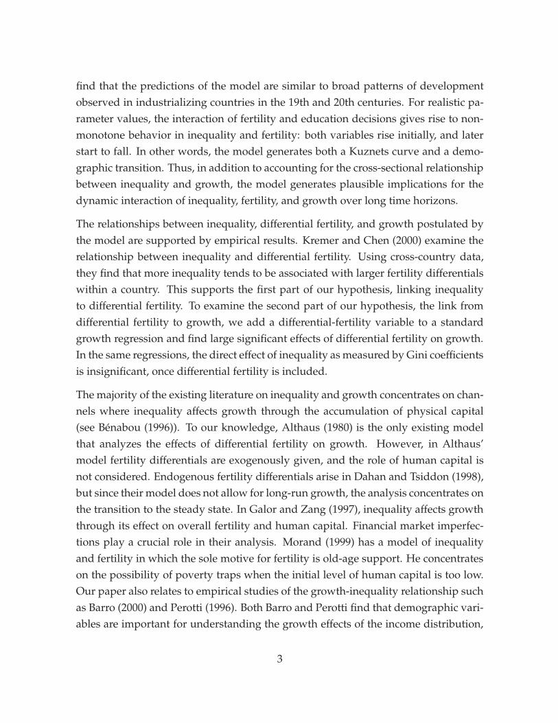
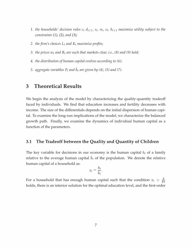
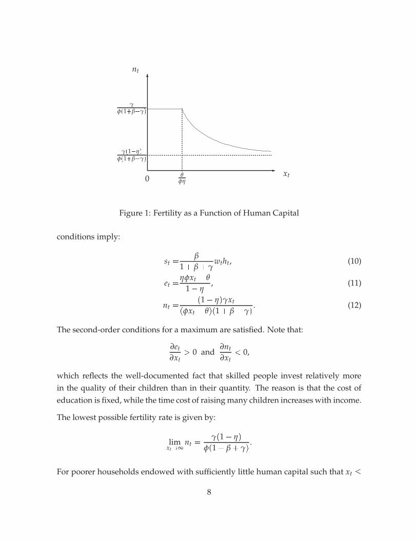
Figure 1: Fertility as a Function of Human Capital

conditions imply:

st =β

1 + β + γwtht, (10)

et =ηφxt � θ

1� η, (11)

nt =(1� η)γxt

(φxt � θ)(1 + β + γ). (12)

The second-order conditions for a maximum are satisfied. Note that:

∂et

∂xt> 0 and

∂nt

∂xt< 0,

which reflects the well-documented fact that skilled people invest relatively morein the quality of their children than in their quantity. The reason is that the cost ofeducation is fixed, while the time cost of raising many children increases with income.

The lowest possible fertility rate is given by:

limxt!∞

nt =γ(1� η)

φ(1 + β + γ).

For poorer households endowed with sufficiently little human capital such that xt �

8

θφη holds, the optimal choice for education et is zero. The first-order conditions implyequation (10) and:

et = 0, (13)

nt =γ

φ(1 + β + γ). (14)

Once a household is at the corner solution and the choice for education is zero, fertil-ity no longer increases as the human capital endowment falls.

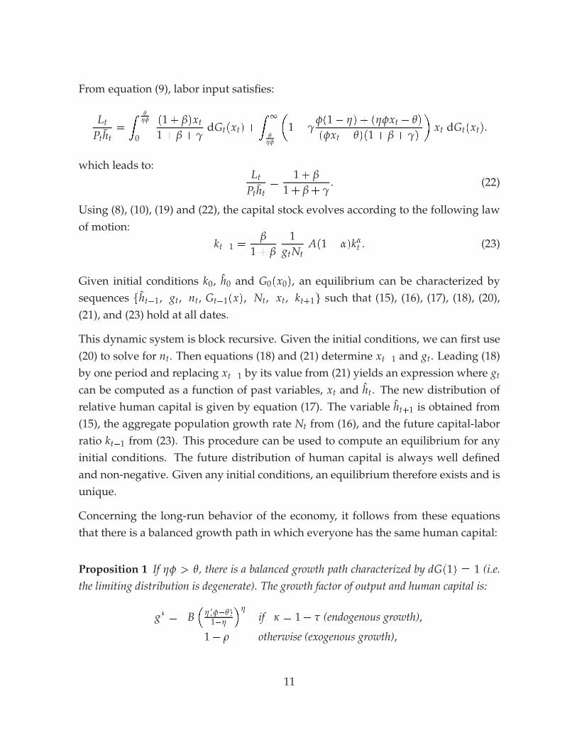
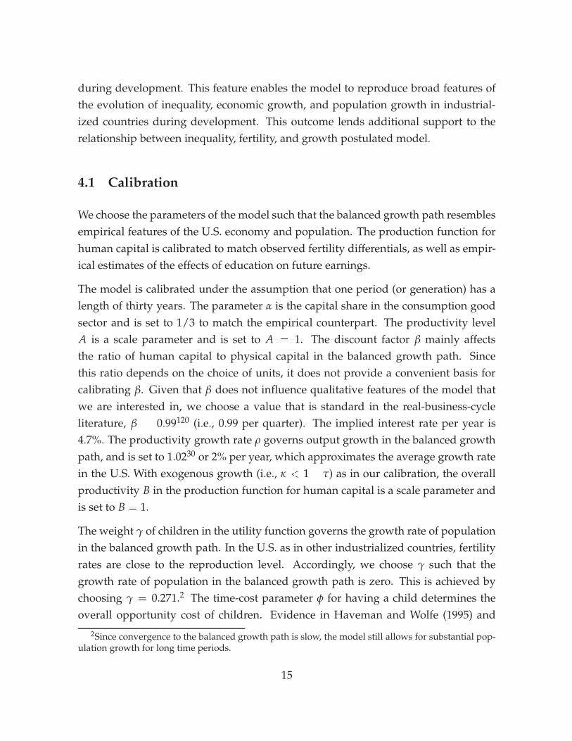
Fertility as a function of human capital is plotted in Figure 1. The horizontal part ofthe relationship corresponds to the range of human capital which leads to a choiceof zero for education et. Fertility depends negatively on human capital and moveswithin a finite interval. The upper bound on the fertility differential is given by:

limxt!0 nt

limxt!∞ nt=

11� η

.

This relationship will turn out to be helpful to interpret the role of the parameter η

and to calibrate its value.

The results derived so far reflect the main effects of inequality on growth that we areinterested in. Assuming that all dynasties choose positive levels of education, equa-tion (11) shows that education is a linear function of relative human capital. If thedispersion of human capital increases for a given average level of human capital, thislinearity implies that the average education choice will still be the same. However,since the production function for human capital is concave in education, future aver-age human capital will be lower if the distribution of human capital is less equal. Thiswould be true even if fertility were constant across families with different human cap-ital levels. The fact that fertility is actually higher for people with low human capitalgreatly amplifies the negative effect of inequality on human capital accumulation.

3.2 The Balanced Growth Path

To analyze the dynamic behavior of the economy, it is useful to rewrite the equilib-rium conditions in terms of variables that are constant in the balanced growth path.

9

The capital/labor ratio kt, the growth rate of average human capital gt, the popula-tion growth rate Nt, and the deflated level of average human capital ht are definedby:

kt �Kt

Lt, gt �

ht+1

ht, Nt �

Pt+1

Pt, ht �

ht

(1 + ρ)t .

We also need to define the distribution of the relative human capital levels:

Gt(xt) � Ft(xtht).

Rewriting equations (4), (5), (6) and (7) in terms of the stationary variables leads to:

ht+1 =gt

1 + ρht (15)

Nt =

Z ∞

0nt dGt(xt), (16)

Gt+1(x) =1

Nt

Z ∞

0nt I(xt+1 � x) dGt(xt), (17)

1 =

Z ∞

0xt dGt(xt). (18)

Prices follow from the competitive behavior of firms, which leads to equalization ofmarginal costs and productivities:

wt = A(1� α)kαt , (19)

Rt = Aαkα�1t .

Schooling and fertility decisions are given by (13) and (14) for xt < θ/(ηφ) and by(11) and (12) otherwise. The number of children for an adult with relative humancapital xt is thus given by:

nt = min�

(1� η)γxt

(φxt � θ)(1 + β + γ),

γ

φ(1 + β + γ)

�. (20)

From equation (3), the children’s human capital is given by:

xt+1 =Bxτ

tgt

�θ + max

�0,

ηφxt � θ

1� η

��η

(ht)τ+κ�1. (21)

10

From equation (9), labor input satisfies:

Lt

Ptht=

Z θηφ

0

(1 + β)xt

1 + β + γdGt(xt) +

Z ∞

θηφ

�1� γ

φ(1� η) + (ηφxt � θ)

(φxt � θ)(1 + β + γ)

�xt dGt(xt).

which leads to:Lt

Ptht=

1 + β

1 + β + γ. (22)

Using (8), (10), (19) and (22), the capital stock evolves according to the following lawof motion:

kt+1 =β

1 + β

1gtNt

A(1� α)kαt . (23)

Given initial conditions k0, h0 and G0(x0), an equilibrium can be characterized bysequences fht+1, gt, nt, Gt+1(x), Nt, xt, kt+1g such that (15), (16), (17), (18), (20),(21), and (23) hold at all dates.

This dynamic system is block recursive. Given the initial conditions, we can first use(20) to solve for nt. Then equations (18) and (21) determine xt+1 and gt. Leading (18)by one period and replacing xt+1 by its value from (21) yields an expression where gt

can be computed as a function of past variables, xt and ht. The new distribution ofrelative human capital is given by equation (17). The variable ht+1 is obtained from(15), the aggregate population growth rate Nt from (16), and the future capital-laborratio kt+1 from (23). This procedure can be used to compute an equilibrium for anyinitial conditions. The future distribution of human capital is always well definedand non-negative. Given any initial conditions, an equilibrium therefore exists and isunique.

Concerning the long-run behavior of the economy, it follows from these equationsthat there is a balanced growth path in which everyone has the same human capital:

Proposition 1 If ηφ > θ, there is a balanced growth path characterized by dG(1) = 1 (i.e.the limiting distribution is degenerate). The growth factor of output and human capital is:

g? = B�

η(φ�θ)1�η

�ηif κ = 1� τ (endogenous growth),

1 + ρ otherwise (exogenous growth),

11

and the growth factor of population is:

N? =(1� η)γ

(φ � θ)(1 + β + γ).

Proof: See Appendix A.

Q.E.D.

Along this balanced growth path, there is no longer any inequality among house-holds. This holds because we have assumed that households differ only in their initiallevel of human capital. If we had introduced ability shocks on top of an unequal ini-tial distribution of human capital, inequality would persist along the balanced growthpath. We abstract from idiosyncratic shocks in the presentation of the model, sincethey do not play a role in the channel from inequality to growth that we are inter-ested in. However, shocks can influence the long-run dynamic behavior of the model.Therefore we introduce ability shocks as an extension in Section 4.3 below.

We will assume ηφ > θ from here on. We now consider the dynamics of the humancapital of an individual dynasty (of mass zero) around an aggregate balanced growthpath. This will be useful to understand the role of the parameter τ for the dynamicproperties of the model.

3.3 The Dynamics of Individual Human Capital

To study the dynamics of individual human capital, we assume that the economy ison a balanced growth path, so that the growth rate of average human capital is con-stant over time: gt = g?. We focus on the effect of the parameter τ on the dynamics ofindividual human capital. We consider the function xt+1 � xt = Ψ(xt; τ) (the changein relative human capital xt as a function of xt and τ), which is given by:

Ψ(x; τ) =

�1� η

η(φ � θ)

�η

xτ

�θ + max

�0,

ηφx � θ

1� η

��η

� x. (24)

As shown in Appendix B, Ψ(xt; τ) is obtained from equation (21) after replacingg? and h by their steady-state values. Note that in the endogenous and exogenousgrowth cases the function Ψ(x; τ) turns out to be the same.

12

-

6

.................

.............................τττ

x

1

6

??

6

? ?

66

6

.................θφη

...........................................................η

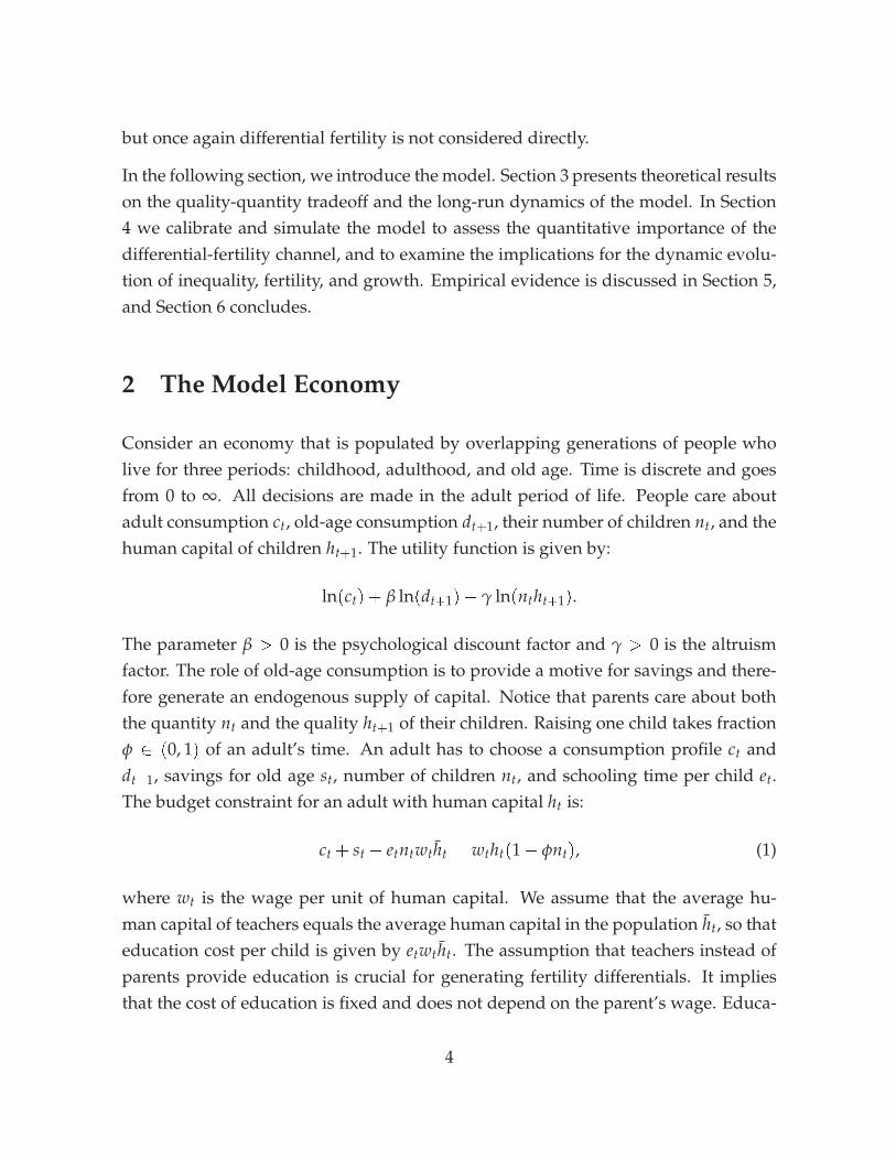
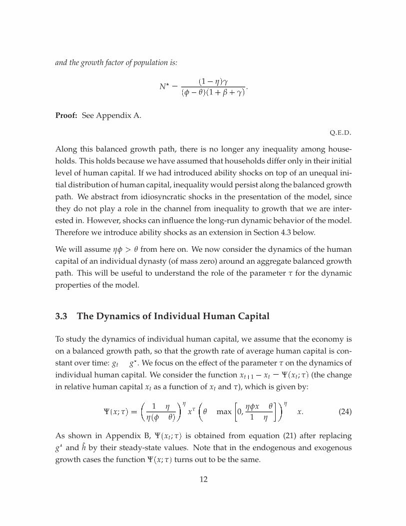
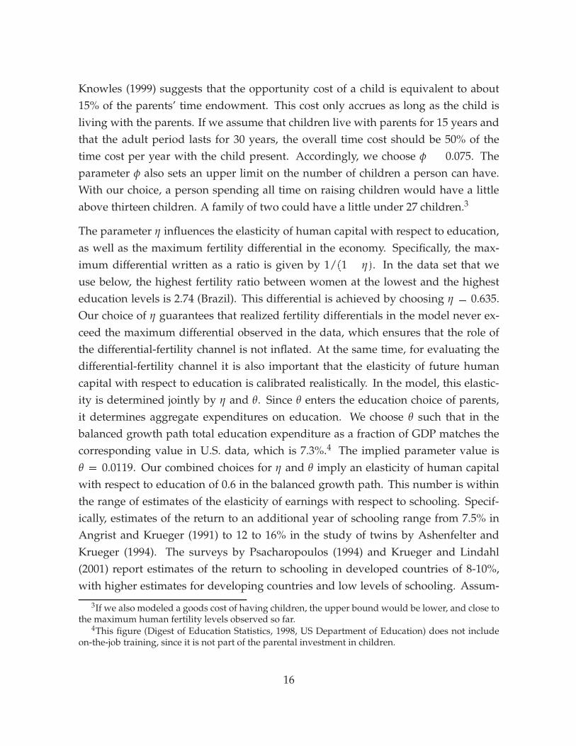
Figure 2: Steady States as a Function of τ

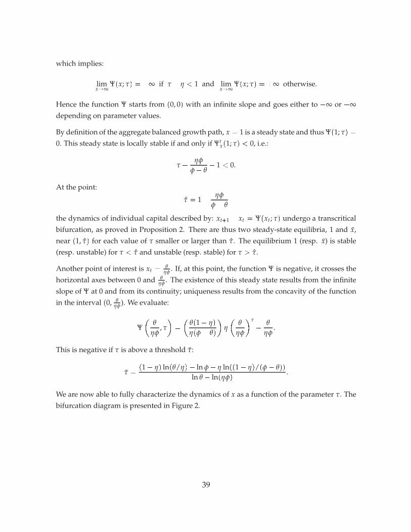
A detailed study of Ψ(xt; τ) is performed in Appendix B. A complete characterizationof the dynamics of xt as a function of the parameter τ is presented in the bifurcationdiagram in Figure 2. The steady states x are represented on the vertical axis as afunction of τ. For small τ there is only one steady state, x = 1, which is globallystable. Once τ reaches a threshold τ (given in the appendix) two additional steadystates appear. The lower one is stable and the second is unstable. This thresholdarises at the point where the cutoff value for an interior solution is a steady state ofthe individual dynamics. Moreover:

Proposition 2 At the point:

τ = 1�ηφ

φ � θ

the dynamics of individual capital described by xt+1 � xt = Ψ(xt; τ) undergo a transcriticalbifurcation. There are two steady-state equilibria, 1 and x, near (1, τ) for each value of τ

smaller or larger than τ. The equilibrium 1 (resp. x) is stable (resp. unstable) for τ < τ andunstable (resp. stable) for τ > τ.

Proof: We check the five conditions that define such a bifurcation in Wiggins (1990),p. 365:

Ψ(1, τ) = 0, Ψ0

x(1, τ) = 0, Ψ0

τ(1, τ) = 0,

13

Ψ00

xx(1, τ) = �ηθφ

(φ � θ)2 6= 0, Ψ00

xτ(1, τ) = 1 6= 0.

Q.E.D.

This bifurcation occurs when an unstable and a stable fixed point collide and ex-change stability. That is, the unstable fixed point becomes stable and vice versa.1

When τ increases beyond τ, the high steady state increases and then vanishes onceτ > η. Thus, for individual dynamics to be stable, it is essential that τ be not toohigh. In the next section, we calibrate the model parameters to data and find that thestable region for τ is the empirically relevant case. The analysis of the dynamics ofxt at given aggregate conditions is helpful to understand the numerical simulationscarried out in the next section.

4 Computational Experiments

The theoretical results in the previous section highlight two channels through whichinequality affects growth in this model. First, inequality in human capital leads toinequality in education, and since the production function for human capital is con-cave, inequality in education lowers future average human capital. Second, peoplewith lower human capital not only choose less education for their children, but also ahigher number of children. This differential-fertility effect increases the weight in thepopulation on families with little education, which also lowers future human capi-tal. The question arises which effect is more important, and how large the effects arequantitatively. To answer this question, we calibrate our model and provide numer-ical simulations of the evolution of fertility, inequality, human capital, and income.The main findings are that the effects of inequality on human capital accumulationand growth are sizable, and that the differential-fertility effect is crucial for generatingthis result.

We also use the calibrated model to analyze the dynamic implications of our theory.Here, a key finding is that for reasonable parameterizations, the model generates a“hump-shape” in inequality and population growth which first increase and then fall

1Note that beyond the bifurcation point the number of fixed points does not change, whereas in asaddle-node bifurcation two fixed points either appear or disappear.

14

during development. This feature enables the model to reproduce broad features ofthe evolution of inequality, economic growth, and population growth in industrial-ized countries during development. This outcome lends additional support to therelationship between inequality, fertility, and growth postulated model.

4.1 Calibration

We choose the parameters of the model such that the balanced growth path resemblesempirical features of the U.S. economy and population. The production function forhuman capital is calibrated to match observed fertility differentials, as well as empir-ical estimates of the effects of education on future earnings.

The model is calibrated under the assumption that one period (or generation) has alength of thirty years. The parameter α is the capital share in the consumption goodsector and is set to 1/3 to match the empirical counterpart. The productivity levelA is a scale parameter and is set to A = 1. The discount factor β mainly affectsthe ratio of human capital to physical capital in the balanced growth path. Sincethis ratio depends on the choice of units, it does not provide a convenient basis forcalibrating β. Given that β does not influence qualitative features of the model thatwe are interested in, we choose a value that is standard in the real-business-cycleliterature, β = 0.99120 (i.e., 0.99 per quarter). The implied interest rate per year is4.7%. The productivity growth rate ρ governs output growth in the balanced growthpath, and is set to 1.0230 or 2% per year, which approximates the average growth ratein the U.S. With exogenous growth (i.e., κ < 1 � τ) as in our calibration, the overallproductivity B in the production function for human capital is a scale parameter andis set to B = 1.

The weight γ of children in the utility function governs the growth rate of populationin the balanced growth path. In the U.S. as in other industrialized countries, fertilityrates are close to the reproduction level. Accordingly, we choose γ such that thegrowth rate of population in the balanced growth path is zero. This is achieved bychoosing γ = 0.271.2 The time-cost parameter φ for having a child determines theoverall opportunity cost of children. Evidence in Haveman and Wolfe (1995) and

2Since convergence to the balanced growth path is slow, the model still allows for substantial pop-ulation growth for long time periods.

15

Knowles (1999) suggests that the opportunity cost of a child is equivalent to about15% of the parents’ time endowment. This cost only accrues as long as the child isliving with the parents. If we assume that children live with parents for 15 years andthat the adult period lasts for 30 years, the overall time cost should be 50% of thetime cost per year with the child present. Accordingly, we choose φ = 0.075. Theparameter φ also sets an upper limit on the number of children a person can have.With our choice, a person spending all time on raising children would have a littleabove thirteen children. A family of two could have a little under 27 children.3

The parameter η influences the elasticity of human capital with respect to education,as well as the maximum fertility differential in the economy. Specifically, the max-imum differential written as a ratio is given by 1/(1 � η). In the data set that weuse below, the highest fertility ratio between women at the lowest and the highesteducation levels is 2.74 (Brazil). This differential is achieved by choosing η = 0.635.Our choice of η guarantees that realized fertility differentials in the model never ex-ceed the maximum differential observed in the data, which ensures that the role ofthe differential-fertility channel is not inflated. At the same time, for evaluating thedifferential-fertility channel it is also important that the elasticity of future humancapital with respect to education is calibrated realistically. In the model, this elastic-ity is determined jointly by η and θ. Since θ enters the education choice of parents,it determines aggregate expenditures on education. We choose θ such that in thebalanced growth path total education expenditure as a fraction of GDP matches thecorresponding value in U.S. data, which is 7.3%.4 The implied parameter value isθ = 0.0119. Our combined choices for η and θ imply an elasticity of human capitalwith respect to education of 0.6 in the balanced growth path. This number is withinthe range of estimates of the elasticity of earnings with respect to schooling. Specif-ically, estimates of the return to an additional year of schooling range from 7.5% inAngrist and Krueger (1991) to 12 to 16% in the study of twins by Ashenfelter andKrueger (1994). The surveys by Psacharopoulos (1994) and Krueger and Lindahl(2001) report estimates of the return to schooling in developed countries of 8-10%,with higher estimates for developing countries and low levels of schooling. Assum-

3If we also modeled a goods cost of having children, the upper bound would be lower, and close tothe maximum human fertility levels observed so far.

4This figure (Digest of Education Statistics, 1998, US Department of Education) does not includeon-the-job training, since it is not part of the parental investment in children.

16

ing that an additional year of schooling raises education expenditure by 20%, thesereturns translate into an earnings elasticity of schooling between 0.4 and 0.8. Theelasticity implied by our parameter choices is exactly in the middle of this range.

The remaining parameters κ and τ do not influence individual decisions, but stillhave an effect on growth rates. The elasticity κ of future human capital with respectto average human capital h can be calibrated to evidence on the effects of the qualityof schooling. We interpret the education choice et as the quantity of schooling (corre-sponding to years of schooling in the data) while h measures the quality of schooling,since it is the average human capital of teachers. Compared to the quantity of school-ing, the quality of schooling (such as spending per pupil at a given level of education)has been shown to have smaller effects on earnings with an elasticity of around 0.1,see Card and Krueger (1996) and Krueger and Lindahl (2001). In line with evidenceon the effect of the quality of education, we set κ = 0.1. Alternatively, κ could also beinterpreted as a measure of human capital externalities. Existing evidence (see Ace-moglu and Angrist 2000 and Krueger and Lindahl 2001) suggests that these external-ities are small as well, i.e., the social return to human capital accumulation is onlyslightly larger than the private return, confirming our low choice of κ. Our results arerobust with respect to the choice of this elasticity in the sense that κ matters only forthe determination of the growth rate of average human capital. Individual decisionsand the evolution of inequality, fertility, and differential fertility are independent ofκ.

The parameter τ determines the direct effect of parental human capital (or, equiva-lently, income) on the children’s human capital. Thus, τ captures the intergenera-tional transmission of ability, as well as human capital formation within the familythat does not work through formal schooling. Empirical studies detect such effects,but they are relatively small. Rosenzweig and Wolpin (1994) find that an additionalyear of the mother’s education at the high school level (roughly a 10% increase ineducation) raises a child’s test scores by 2.4%. Leibowitz (1974) finds that even aftercontrolling for schooling and education of the parents, parental income has a signifi-cant effect on a child’s earnings. A 10% increase in parental income increases a child’sfuture earnings by up to 0.85%. Given that the long-run dynamics of the model aresensitive to the choice of τ, we choose a moderate degree of intergenerational trans-mission of human capital (τ = 0.2) as the baseline case, and provide a sensitivity

17

analysis with respect to alternative choices for τ. For individual dynamics to be sta-ble, τ must not exceed the upper bound τ from Proposition 2. Given our choices forthe other parameters, the upper limit for τ is 0.246, which is well above the calibratedvalue.

In addition to choosing parameters, we also need to set the initial conditions for thesimulations. The overall size of the population is a scale parameter which does notaffect the results, and is therefore set to one. Likewise, the distribution of physicalcapital does not matter, since capital is owned by old people who have nothing leftto decide. We therefore only specify the aggregate value. The initial distributionof human capital follows a log-normal distribution F(µ, σ2), where µ and σ2 are themean and variance of the underlying normal distribution. The parameter µ is set suchthat ht is at its balanced-growth level. We provide simulations for different variancesof the distribution in order to examine the effects of inequality. The initial level ofphysical capital K0 is chosen such that the ratio of physical to human capital is equalto its value in the balanced growth path.5

4.2 Initial Inequality, Fertility, and Growth

As a first computational experiment, we examine the effect of initial inequality ongrowth over the first period. Since a period is in fact a generation, the growth rateshould be interpreted as a thirty-year average. The main findings are that inequalityhas a sizable effect on growth, and that most of this effect is accounted for by theendogenous fertility differential.

Table 1 presents the initial annualized growth rates of human capital g0 and pop-ulation N0, initial inequality I0, and the initial fertility differential D0 for differentvariances of the distribution of human capital. Inequality is measured by the Ginicoefficient I0 computed on the earnings of the working population. Differential fer-tility is the difference between the average fertility of the top quintile and the bottomquintile; this quantity is then multiplied by two to yield a number per woman. Toevaluate the role of differential fertility in our model, we also computed results un-der the assumption of constant, exogenous fertility.

5The effect of inequality on growth is independent of µ and K0; µ and K0 only affect average growthrates.

18

Endogenous Fertility Exogenous Fertility

σ2 g0 N0 I0 D0 g0 N0 I0 D0

0.10 2.00% 0.00% 0.056 0.09 2.00% 0% 0.056 0

0.75 1.26% 0.66% 0.404 1.95 1.87% 0% 0.400 0

1.00 0.80% 1.08% 0.520 2.76 1.78% 0% 0.513 0

1.50 0.01% 1.71% 0.707 2.77 1.53% 0% 0.700 0

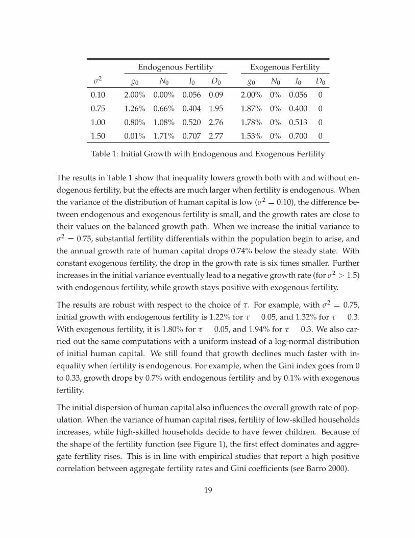
Table 1: Initial Growth with Endogenous and Exogenous Fertility

The results in Table 1 show that inequality lowers growth both with and without en-dogenous fertility, but the effects are much larger when fertility is endogenous. Whenthe variance of the distribution of human capital is low (σ2 = 0.10), the difference be-tween endogenous and exogenous fertility is small, and the growth rates are close totheir values on the balanced growth path. When we increase the initial variance toσ2 = 0.75, substantial fertility differentials within the population begin to arise, andthe annual growth rate of human capital drops 0.74% below the steady state. Withconstant exogenous fertility, the drop in the growth rate is six times smaller. Furtherincreases in the initial variance eventually lead to a negative growth rate (for σ2

> 1.5)with endogenous fertility, while growth stays positive with exogenous fertility.

The results are robust with respect to the choice of τ. For example, with σ2 = 0.75,initial growth with endogenous fertility is 1.22% for τ = 0.05, and 1.32% for τ = 0.3.With exogenous fertility, it is 1.80% for τ = 0.05, and 1.94% for τ = 0.3. We also car-ried out the same computations with a uniform instead of a log-normal distributionof initial human capital. We still found that growth declines much faster with in-equality when fertility is endogenous. For example, when the Gini index goes from 0to 0.33, growth drops by 0.7% with endogenous fertility and by 0.1% with exogenousfertility.

The initial dispersion of human capital also influences the overall growth rate of pop-ulation. When the variance of human capital rises, fertility of low-skilled householdsincreases, while high-skilled households decide to have fewer children. Because ofthe shape of the fertility function (see Figure 1), the first effect dominates and aggre-gate fertility rises. This is in line with empirical studies that report a high positivecorrelation between aggregate fertility rates and Gini coefficients (see Barro 2000).

19

0.2 0.4 0.6 0.8Gini

-0.005

0.005

0.01

0.015

0.02

Growth

Barro’s reg. slope

Exo. fertility

Endog. fertility

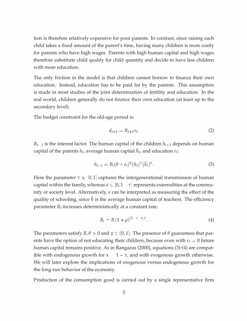
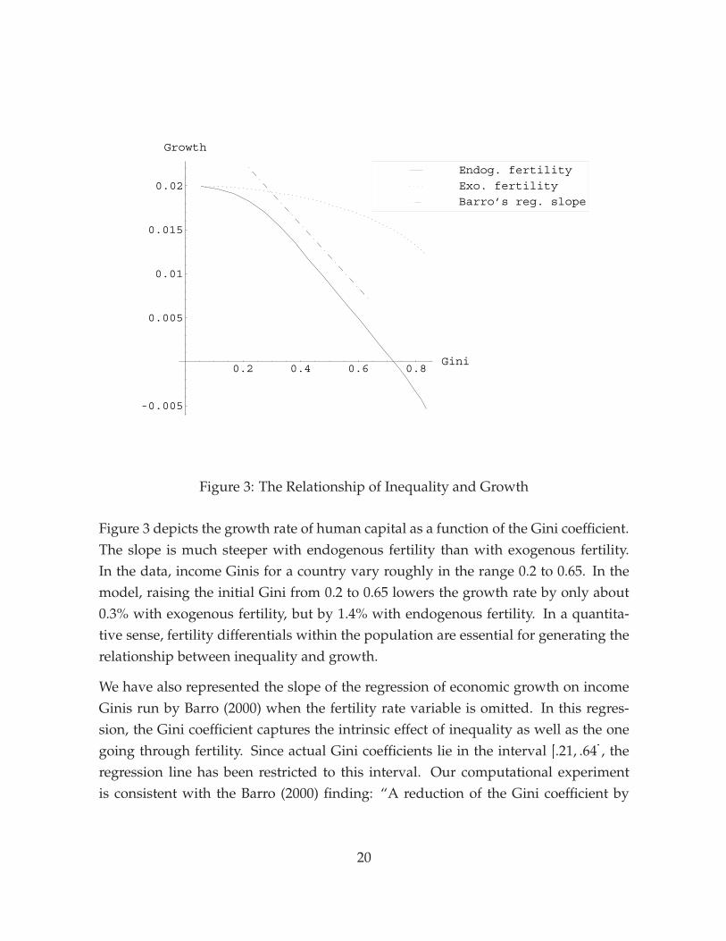
Figure 3: The Relationship of Inequality and Growth

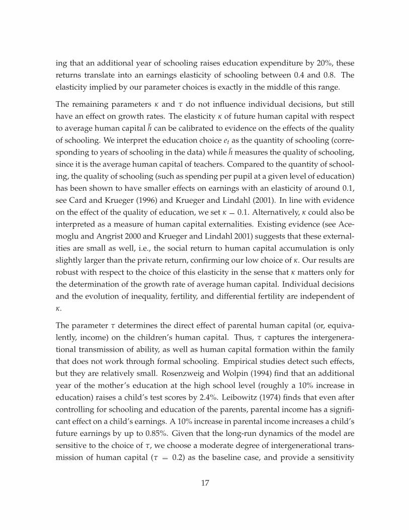
Figure 3 depicts the growth rate of human capital as a function of the Gini coefficient.The slope is much steeper with endogenous fertility than with exogenous fertility.In the data, income Ginis for a country vary roughly in the range 0.2 to 0.65. In themodel, raising the initial Gini from 0.2 to 0.65 lowers the growth rate by only about0.3% with exogenous fertility, but by 1.4% with endogenous fertility. In a quantita-tive sense, fertility differentials within the population are essential for generating therelationship between inequality and growth.

We have also represented the slope of the regression of economic growth on incomeGinis run by Barro (2000) when the fertility rate variable is omitted. In this regres-sion, the Gini coefficient captures the intrinsic effect of inequality as well as the onegoing through fertility. Since actual Gini coefficients lie in the interval [.21, .64], theregression line has been restricted to this interval. Our computational experimentis consistent with the Barro (2000) finding: “A reduction of the Gini coefficient by

20

0.1 would be estimated to raise the growth rate on impact by 0.4 percent per year.”6

Perotti (1996) reports effects of similar magnitude. Our calibrated model is thereforeable to account for most of the empirical relationship between inequality and growth.Since the empirical estimates carry sizable standard errors, the finding does not ruleout that other channels could also play a role, but clearly the differential-fertility effectappears to be important.

4.3 The Dynamics of Inequality, Differential Fertility, and Growth

We now turn to the dynamic implications of our model. So far, we have only an-alyzed the effects of inequality on growth during the initial period. Since in ourdynastic model a period has a length of 30 years, even the initial growth effect ex-tends over a long horizon, and consequently the dynamics of the model are to beinterpreted as changes which occur over a horizon of a century or more. We thereforeevaluate the dynamic behavior of the model relative to the evolution of income, fertil-ity, and inequality in industrializing countries in the last 200 years. A central featureof the data for this period is that the behavior of population growth and inequalityis non-monotone. As a benchmark case, consider England, the first country to in-dustrialize. Fertility rates increased until about 1830 and started to decline rapidlyonly after 1870 (Chesnais 1992). Income inequality followed a similar pattern, withincreasing inequality until about 1870 and a rapid decline afterwards (Williamson1985). The growth rate of income per capita, in contrast, does not display a hump-shape. Growth rates were essentially zero before the industrial revolution and thenincreased slowly throughout the 19th century (Maddison 2001). Similar patterns canbe observed for Western Europe as a whole and, starting a little later, in the UnitedStates.

To evaluate how our model performs relative to these facts, we simulate the model

6The comparison to Barro’s result is complicated by the fact that Barro conditions his estimates oninitial GDP, whereas in our simulations GDP is partly a function of the initial income distribution.Thus, in principle, the simulations pick up the additional effect of changing initial GDP. In practice,however, this effect turns out to be negligible. Initial GDP varies only to the extent that child-rearingtime is not included in GDP, and the resulting differences in GDP across inequality levels are small(up to 0.3%). We computed results with an additional adjustment in average human capital that holdsGDP per worker constant across inequality levels. The results are virtually indistinguishable from theones reported in Figure 3.

21

with the baseline calibration over a horizon of eight periods, corresponding to 240years. The main finding is that for plausible parameters, the model can generate ahump-shape in inequality and the population growth rate that looks very similar tothe data. This is a surprising finding, since unlike most existing theories the modelgenerates the pattern without requiring any exogenous change to the economic en-vironment. We also investigate the behavior of the model if idiosyncratic shocks areadded to the production function for human capital, since for long-run analysis theassumption that the only source of inequality is the initial dispersion in human capitalis less attractive. We find that adding shocks slows growth, but leaves the qualitativebehavior of the model intact. Thus our model turns out to be successful at accountingfor both the cross-sectional relationship between inequality and growth, and the dy-namic interaction between inequality, fertility, and growth over long time horizons.

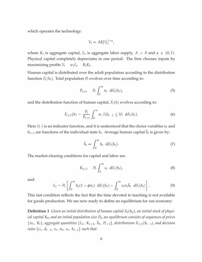
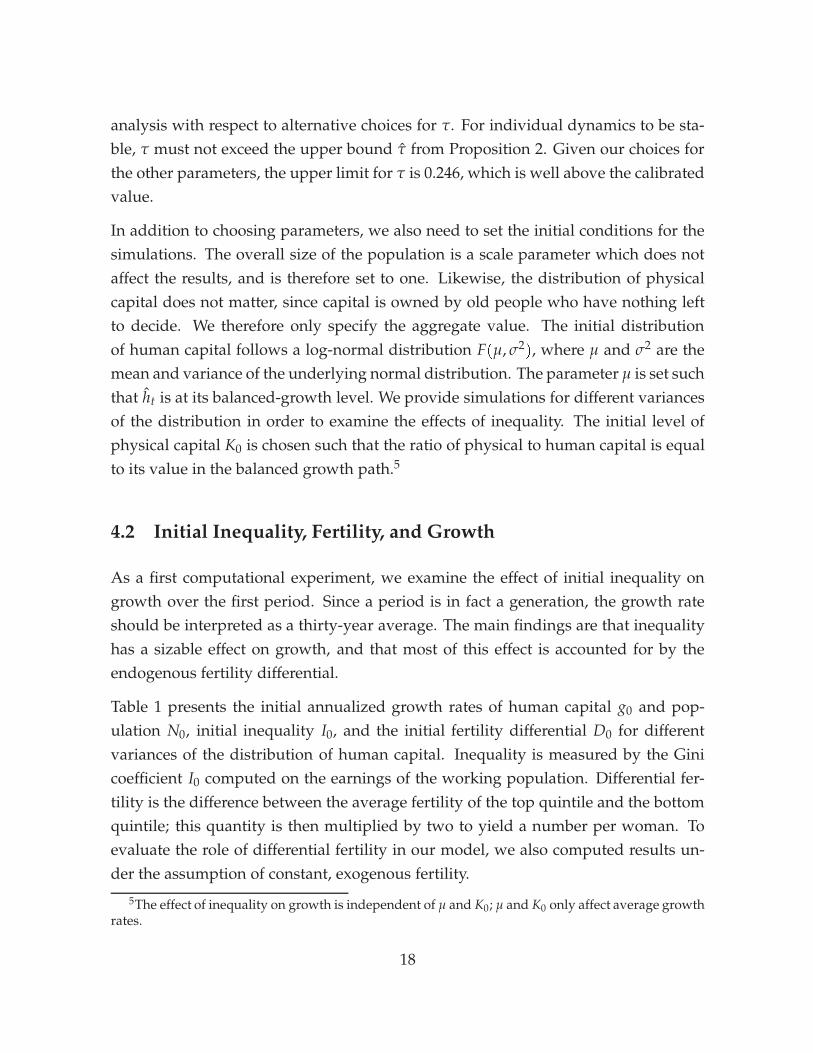
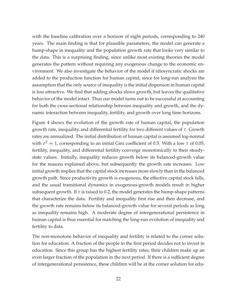
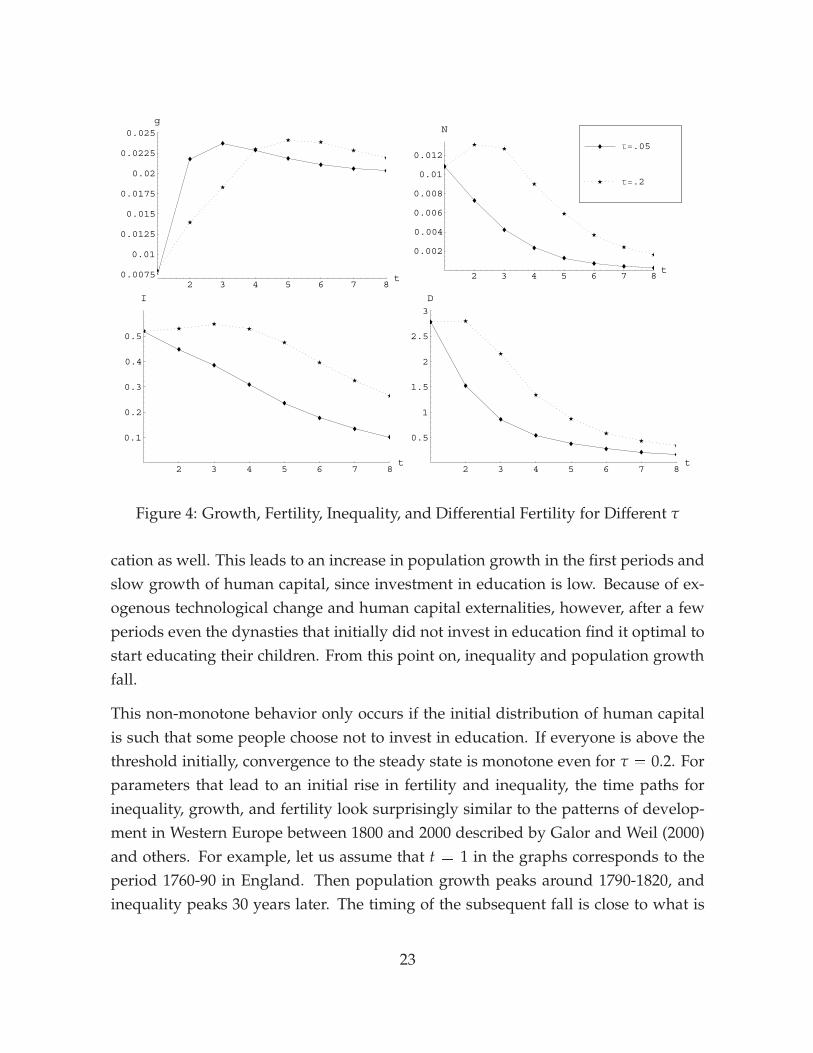
Figure 4 shows the evolution of the growth rate of human capital, the populationgrowth rate, inequality, and differential fertility for two different values of τ. Growthrates are annualized. The initial distribution of human capital is assumed log-normalwith σ2 = 1, corresponding to an initial Gini coefficient of 0.5. With a low τ of 0.05,fertility, inequality, and differential fertility converge monotonically to their steady-state values. Initially, inequality reduces growth below its balanced-growth valuefor the reasons explained above, but subsequently the growth rate increases. Lowinitial growth implies that the capital stock increases more slowly than in the balancedgrowth path. Since productivity growth is exogenous, the effective capital stock falls,and the usual transitional dynamics in exogenous-growth models result in highersubsequent growth. If τ is raised to 0.2, the model generates the hump-shape patternsthat characterize the data. Fertility and inequality first rise and then decrease, andthe growth rate remains below its balanced-growth value for several periods as longas inequality remains high. A moderate degree of intergenerational persistence inhuman capital is thus essential for matching the long-run evolution of inequality andfertility to data.

The non-monotone behavior of inequality and fertility is related to the corner solu-tion for education. A fraction of the people in the first period decides not to invest ineducation. Since this group has the highest fertility rates, their children make up aneven larger fraction of the population in the next period. If there is a sufficient degreeof intergenerational persistence, these children will be at the corner solution for edu-

22

2 3 4 5 6 7 8t0.0075

0.01

0.0125

0.015

0.0175

0.02

0.0225

0.025g

2 3 4 5 6 7 8t

0.002

0.004

0.006

0.008

0.01

0.012

N

Τ�.2

Τ�.05

2 3 4 5 6 7 8t

0.1

0.2

0.3

0.4

0.5

I

2 3 4 5 6 7 8t

0.5

1

1.5

2

2.5

3D

Figure 4: Growth, Fertility, Inequality, and Differential Fertility for Different τ

cation as well. This leads to an increase in population growth in the first periods andslow growth of human capital, since investment in education is low. Because of ex-ogenous technological change and human capital externalities, however, after a fewperiods even the dynasties that initially did not invest in education find it optimal tostart educating their children. From this point on, inequality and population growthfall.

This non-monotone behavior only occurs if the initial distribution of human capitalis such that some people choose not to invest in education. If everyone is above thethreshold initially, convergence to the steady state is monotone even for τ = 0.2. Forparameters that lead to an initial rise in fertility and inequality, the time paths forinequality, growth, and fertility look surprisingly similar to the patterns of develop-ment in Western Europe between 1800 and 2000 described by Galor and Weil (2000)and others. For example, let us assume that t = 1 in the graphs corresponds to theperiod 1760-90 in England. Then population growth peaks around 1790-1820, andinequality peaks 30 years later. The timing of the subsequent fall is close to what is

23

observed in the data. For the hump to occur, however, τ cannot be too small, i.e., weneed some degree of intergenerational persistence in human capital and earnings.7

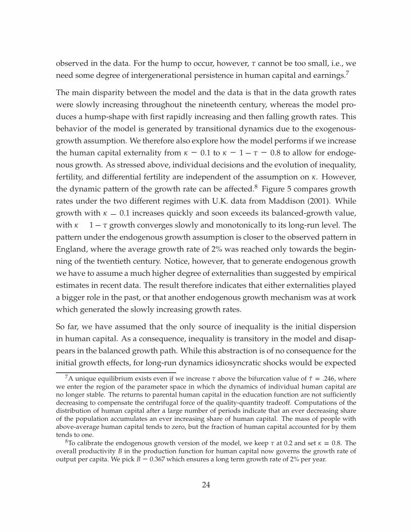
The main disparity between the model and the data is that in the data growth rateswere slowly increasing throughout the nineteenth century, whereas the model pro-duces a hump-shape with first rapidly increasing and then falling growth rates. Thisbehavior of the model is generated by transitional dynamics due to the exogenous-growth assumption. We therefore also explore how the model performs if we increasethe human capital externality from κ = 0.1 to κ = 1 � τ = 0.8 to allow for endoge-nous growth. As stressed above, individual decisions and the evolution of inequality,fertility, and differential fertility are independent of the assumption on κ. However,the dynamic pattern of the growth rate can be affected.8 Figure 5 compares growthrates under the two different regimes with U.K. data from Maddison (2001). Whilegrowth with κ = 0.1 increases quickly and soon exceeds its balanced-growth value,with κ = 1� τ growth converges slowly and monotonically to its long-run level. Thepattern under the endogenous growth assumption is closer to the observed pattern inEngland, where the average growth rate of 2% was reached only towards the begin-ning of the twentieth century. Notice, however, that to generate endogenous growthwe have to assume a much higher degree of externalities than suggested by empiricalestimates in recent data. The result therefore indicates that either externalities playeda bigger role in the past, or that another endogenous growth mechanism was at workwhich generated the slowly increasing growth rates.

So far, we have assumed that the only source of inequality is the initial dispersionin human capital. As a consequence, inequality is transitory in the model and disap-pears in the balanced growth path. While this abstraction is of no consequence for theinitial growth effects, for long-run dynamics idiosyncratic shocks would be expected

7A unique equilibrium exists even if we increase τ above the bifurcation value of τ = .246, wherewe enter the region of the parameter space in which the dynamics of individual human capital areno longer stable. The returns to parental human capital in the education function are not sufficientlydecreasing to compensate the centrifugal force of the quality-quantity tradeoff. Computations of thedistribution of human capital after a large number of periods indicate that an ever decreasing shareof the population accumulates an ever increasing share of human capital. The mass of people withabove-average human capital tends to zero, but the fraction of human capital accounted for by themtends to one.

8To calibrate the endogenous growth version of the model, we keep τ at 0.2 and set κ = 0.8. Theoverall productivity B in the production function for human capital now governs the growth rate ofoutput per capita. We pick B = 0.367 which ensures a long term growth rate of 2% per year.

24

2 3 4 5 6 7 8t

0.005

0.01

0.015

0.02

0.025g

data

Κ�0.1

Κ�1�Τ

Figure 5: Exogenous versus Endogenous Growth

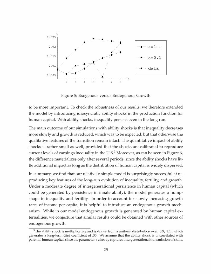
to be more important. To check the robustness of our results, we therefore extendedthe model by introducing idiosyncratic ability shocks in the production function forhuman capital. With ability shocks, inequality persists even in the long run.

The main outcome of our simulations with ability shocks is that inequality decreasesmore slowly and growth is reduced, which was to be expected, but that otherwise thequalitative features of the transition remain intact. The quantitative impact of abilityshocks is rather small as well, provided that the shocks are calibrated to reproducecurrent levels of earnings inequality in the U.S.9 Moreover, as can be seen in Figure 6,the difference materializes only after several periods, since the ability shocks have lit-tle additional impact as long as the distribution of human capital is widely dispersed.

In summary, we find that our relatively simple model is surprisingly successful at re-producing key features of the long-run evolution of inequality, fertility, and growth.Under a moderate degree of intergenerational persistence in human capital (whichcould be generated by persistence in innate ability), the model generates a hump-shape in inequality and fertility. In order to account for slowly increasing growthrates of income per capita, it is helpful to introduce an endogenous growth mech-anism. While in our model endogenous growth is generated by human capital ex-ternalities, we conjecture that similar results could be obtained with other sources ofendogenous growth.

9The ability shock is multiplicative and is drawn from a uniform distribution over [0.9, 1.1], whichgenerates a long-term Gini coefficient of .35. We assume that the ability shock is uncorrelated withparental human capital, since the parameter τ already captures intergenerational transmission of skills.

25

2 3 4 5 6 7 8t

0.01

0.0125

0.015

0.0175

0.02

0.0225

g

abil. shocks

baseline

2 3 4 5 6 7 8t

0.3

0.35

0.4

0.45

0.5

0.55I

Figure 6: Growth and Inequality with and without Ability Shocks

Our results complement existing theories of long-run growth. Relative to the liter-ature, the main novelty is that we link the evolution of growth and population tothe income distribution. In contrast, the models developed by Hansen and Prescott(1999), Galor and Weil (2000), and Boucekkine, de la Croix, and Licandro (2002) ab-stract from distributional issues.10 We find that allowing for inequality in humancapital combined with endogenous fertility and education choice generates realisticpredictions for inequality, fertility, and growth in a simple and natural way. Galorand Weil (2000) generate a hump in fertility by introducing a subsistence level of con-sumption, but the evolution of the income distribution is not explained. In Hansenand Prescott (1999) fertility is exogenous, so neither the hump in fertility nor in in-equality are accounted for. A limitation of our approach is that we take the initialconditions at the start of the industrial revolution as given. For a full account of theevolution of the economy from pre-industrial stagnation to modern growth we wouldhave to add an element to the model that generates the initial stagnation phase. Wesuspect that this could be done along the lines of Galor and Weil (2000) or Hansenand Prescott (1999), but the extension is beyond the scope of the current paper.

A main implication of our dynamic analysis for the inequality-growth relationship isthat the relationship can be modified by transitional dynamics. Since inequality firstincreases and then decreases during the transition, inequality does not map one-to-one into growth rates. In the empirical analysis, it is therefore important to control

10Doepke (2001) has a model of the industrial revolution and the demographic transition which doesallow for inequality. However, since there are only two types of agents, the income distribution hasjust two points. A hump in inequality arises only if there are exogenous policy changes.

26

for transitional dynamics to isolate the role of the differential-fertility channel.

5 Empirical Evidence

Can the relationships between inequality, differential fertility, and growth postulatedby our model be supported by empirical evidence? The first part of our hypothe-sis, that income inequality leads to high fertility differentials, has been analyzed byKremer and Chen (2000). In line with our conjecture, they find that Gini coefficientshave a significant and sizable positive correlation with fertility differentials. In thissection we examine the second part of our hypothesis, the link from fertility differ-entials to growth. Our approach is to introduce a differential fertility variable intoa standard growth regression. The analysis is designed to be comparable to recentempirical studies of inequality and growth. As predicted by our model, we find thatdifferential fertility has a negative effect on growth. Moreover, when the differentialfertility variable is present, the Gini variable is no longer significant in the regression.

5.1 Data

Our sample contains 68 countries for which data on fertility differentials is available.The dependent variable (GR) in all regressions is the average annual growth rate ofGDP per capita over the periods 1960 to 1976 or 1976 to 1992 (the period depends onthe availability of fertility data). The GDP data is from the Penn World Tables, andgrowth rates are continuously compounded and expressed as percentages.11 Since weare interested in long-run growth, we chose the longest sub-sample periods availablein the Penn World Tables.

Following Kremer and Chen (2000), for fertility differentials we rely on informationfrom the World Fertility Survey and the Demographic and Health Surveys on totalfertility rates by women’s educational attainment (see Jones 1982, United Nations1987, Mboup and Saha 1998, and United Nations 1995). For countries that partici-pated in the World Fertility Survey, the independent variable is growth in GDP per

11For countries where data from 1960 and/or 1992 was not available, we computed growth ratesover the closest available interval.

27

Sample Observations Variable Mean S.D. Min Max

1960-1976 40 GR 1.95 3.65 -5.75 8.44

GINI 44.32 11.14 23.38 68.00

TFR 5.56 1.89 2.02 7.93

DTFR 2.23 1.56 0.22 5.30

1976-1992 43 GR 0.39 1.89 -3.46 4.97

GINI 45.91 9.56 28.90 69.00

TFR 6.06 1.08 3.37 8.00

DTFR 2.41 0.99 0.10 4.50

Total 83 GR 1.14 2.97 -5.75 8.44

GINI 45.14 10.32 23.38 69.00

TFR 5.82 1.54 2.02 8.00

DTFR 2.32 1.29 0.10 5.30

Table 2: Descriptive Statistics

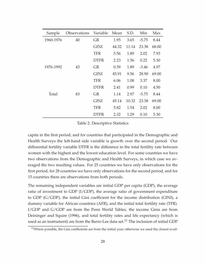
capita in the first period, and for countries that participated in the Demographic andHealth Surveys the left-hand side variable is growth over the second period. Ourdifferential fertility variable DTFR is the difference in the total fertility rate betweenwomen with the highest and the lowest education level. For some countries we havetwo observations from the Demographic and Health Surveys, in which case we av-eraged the two resulting values. For 25 countries we have only observations for thefirst period, for 28 countries we have only observations for the second period, and for15 countries there are observations from both periods.

The remaining independent variables are initial GDP per capita (GDP), the averageratio of investment to GDP (I/GDP), the average ratio of government expenditureto GDP (G/GDP), the initial Gini coefficient for the income distribution (GINI), adummy variable for African countries (AFR), and the initial total fertility rate (TFR).I/GDP and G/GDP are from the Penn World Tables, the income Ginis are fromDeininger and Squire (1996), and total fertility rates and life expectancy (which isused as an instrument) are from the Barro-Lee data set.12 The inclusion of initial GDP

12Where possible, the Gini coefficients are from the initial year; otherwise we used the closest avail-

28

and the investment ratio is important to control for transitional dynamics.

One shortcoming of the data set is that the observations on fertility differentials areclose to the end of the period over which we compute growth rates. Since the fertilityobservations are five-year averages and result from decisions and actions taken evenearlier, the endogeneity problem is not too severe. We correct for potential endogene-ity of the differentials by using instrumental variables.

Table 2 provides descriptive statistics for the main variables in our analysis. Thetwo sub-samples are similar, except that the average growth rate is much lower inthe second sample. Since we will allow for different constant terms in the two sub-samples, this difference will not play a role in the results. These will thus reflect cross-sectional differences among countries, as well as variation over time within countries.

5.2 Estimation Results

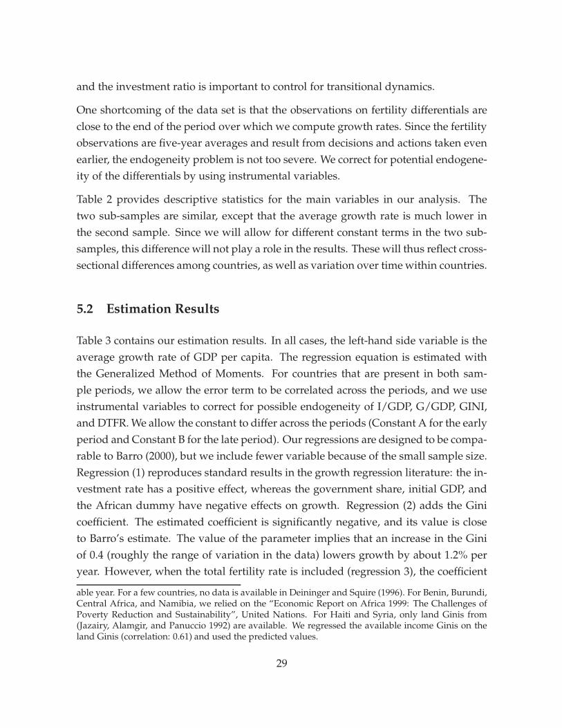
Table 3 contains our estimation results. In all cases, the left-hand side variable is theaverage growth rate of GDP per capita. The regression equation is estimated withthe Generalized Method of Moments. For countries that are present in both sam-ple periods, we allow the error term to be correlated across the periods, and we useinstrumental variables to correct for possible endogeneity of I/GDP, G/GDP, GINI,and DTFR. We allow the constant to differ across the periods (Constant A for the earlyperiod and Constant B for the late period). Our regressions are designed to be compa-rable to Barro (2000), but we include fewer variable because of the small sample size.Regression (1) reproduces standard results in the growth regression literature: the in-vestment rate has a positive effect, whereas the government share, initial GDP, andthe African dummy have negative effects on growth. Regression (2) adds the Ginicoefficient. The estimated coefficient is significantly negative, and its value is closeto Barro’s estimate. The value of the parameter implies that an increase in the Giniof 0.4 (roughly the range of variation in the data) lowers growth by about 1.2% peryear. However, when the total fertility rate is included (regression 3), the coefficient

able year. For a few countries, no data is available in Deininger and Squire (1996). For Benin, Burundi,Central Africa, and Namibia, we relied on the “Economic Report on Africa 1999: The Challenges ofPoverty Reduction and Sustainability”, United Nations. For Haiti and Syria, only land Ginis from(Jazairy, Alamgir, and Panuccio 1992) are available. We regressed the available income Ginis on theland Ginis (correlation: 0.61) and used the predicted values.

29

Independent Regression

variable (1) (2) (3) (4)

Constant A 12.35?? (1.31) 12.79?? (1.33) 15.30?? (1.46) 13.92?? (1.69)

Constant B 10.41?? (1.36) 10.98?? (1.38) 13.40?? (1.45) 12.18?? (1.63)

ln(GDP) -1.33?? (0.17) -1.21?? (0.16) -1.37?? (0.15) -1.55?? (0.20)

I/GDP 0.14?? (0.02) 0.13?? (0.02) 0.07?? (0.03) 0.08?? (0.04)

G/GDP - 0.08?? (0.03) -0.07?? (0.03) -0.05? (0.03) -0.05? (0.03)

AFR -1.75?? (0.35) -1.80?? (0.35) -1.95?? (0.32) -2.41?? (0.44)

GINI -0.03?? (0.01) 0.02 (0.03) 0.06 (0.05)

ln(TFR) -1.84?? (0.87) -1.01 (1.01)

ln(DTFR) -1.22?? (0.50)

Jtest 17.71 [0.48] 17.11 [0.45] 16.79 [0.40] 9.58 [0.85]

LR1 5.53 [0.01]

LR2 2.08 [0.35]

The dependent variable is the growth rate of real per capita GDP. Estimation by GMM. The in-struments are: constant, log of initial GDP per capita, log of initial GDP per capita squared, initial in-vestment/GDP ratio, initial government spending/GDP ratio, initial fertility, initial fertility squared,initial life expectancy, initial life expectancy squared, Africa dummy, and the tropics and access to thesea variables of Sachs and Warner (1997).

Standard errors are reported in parentheses. These are based on the heteroscedastic-consistentcovariance matrix of Newey-West. One star indicates significance at the 10%, two stars indicate signif-icance at the 5% level.

Jtest is the test for over-identifying restrictions of Hansen (1982), asymptotically χ2 distributedwith n degrees of freedom, where n is the number of over-identifying restrictions. Correspondingp�values are reported in brackets.

LR1 is a quasi-likelihood ratio test for the absence of the differential fertility in the equation. LR2is the test for the absence of both Gini and total fertility. As suggested by Gallant (1987), they arecomputed as the normalized difference between the constrained objective function and the uncon-strained one. The constrained estimation is computed with the weighting matrix provided by theunconstrained estimation. The corresponding p�values are reported in brackets.

Table 3: Generalized Method of Moments Estimation

30

Independent Regression

variable (1) (2) (3) (4)

Constant A 9.88 (10.1) -6.70 (17.5) -3.31 (18.8) 6.72 (19.9)

Constant B 7.95 (10.1) -8.48 (17.4) -4.77 (18.6) 479 (19.7)

ln(GDP) -0.65 (2.73) 4.65 (4.12) 2.37 (4.09) 1.39 (4.26)

ln(GDP)2 -0.04 (0.18) -0.40 (0.24) -0.15 (0.20) -0.26 (0.22)

I/GDP 0.14?? (0.02) 0.10?? (0.02) 0.07? (0.04) 0.08?? (0.04)

G/GDP - 0.08?? (0.03) -0.08?? (0.03) -0.07?? (0.04) -0.07?? (0.03)

AFR -1.73?? (0.36) -1.64?? (0.46) -2.23?? (0.43) -2.10?? (0.52)

GINI -0.13 (0.22) 0.31 (0.27) -0.18 (0.37)

ln(GDP)*GINI/100 -0.01 (0.03) -0.04 (0.04) 0.03 (0.05)

ln(TFR) -2.20 ? (1.13) 0.14 (1.51)

ln(DTFR) -1.56?? (0.68)

Jtest 17.63 [0.41] 13.87 [0.54] 16.58 [0.28] 8.38 [0.82]

LR1 5.54 [0.02]

LR2 0.52 [0.77]

The dependent variable is the growth rate of real per capita GDP. Estimation by GMM. Instrumentsas in Table 3.

Table 4: GMM Estimation with Squared GDP and Cross Effects

31

on the Gini coefficient changes sign and becomes insignificant, which is also in linewith Barro (2000).

Regression (4) includes the differential-fertility variable. The coefficient on differen-tial fertility is significantly negative. The point estimate implies that an increase inthe fertility differential from one to two would lower growth by 0.8% per year. Withdifferential fertility included, the coefficients on both Gini and TFR are insignificant,and the point estimate on the Gini is positive.

Based on the results in Section 4, our model predicts that Gini, total fertility, and dif-ferential fertility should all be equally negatively related to growth. It is therefore notclear why the coefficients on the Gini and the total fertility rate become insignificantonce differential fertility is introduced. One possibility is that inequality and totalfertility are influenced by other factors which do not affect growth, while differen-tial fertility is observed with less noise. A second possibility is that total fertility andinequality have other effects on growth, which are not present in our model and donot work through differential fertility. If some of these effects on growth are positiveand therefore offset the negative effects, it would be plausible that the overall effect oftotal fertility and the Gini becomes insignificant once the differential-fertility channelis controlled for.

Hansen’s J-test measures how close the residuals are to being orthogonal to the in-strument set. It can be seen as a global specification test. The degrees of freedomequal the number of restrictions imposed by the orthogonality conditions. These re-strictions are never rejected at the 5% level. Moreover, there is a large improvementin the value of the test when differential fertility is introduced. The significance ofthe differential fertility variable is verified both by its t-statistic and by the quasi-likelihood ratio test LR1. The test LR2 of joint insignificance of GINI and TFR is notrejected.

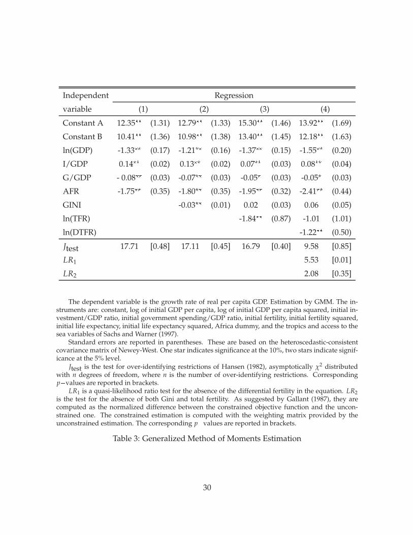
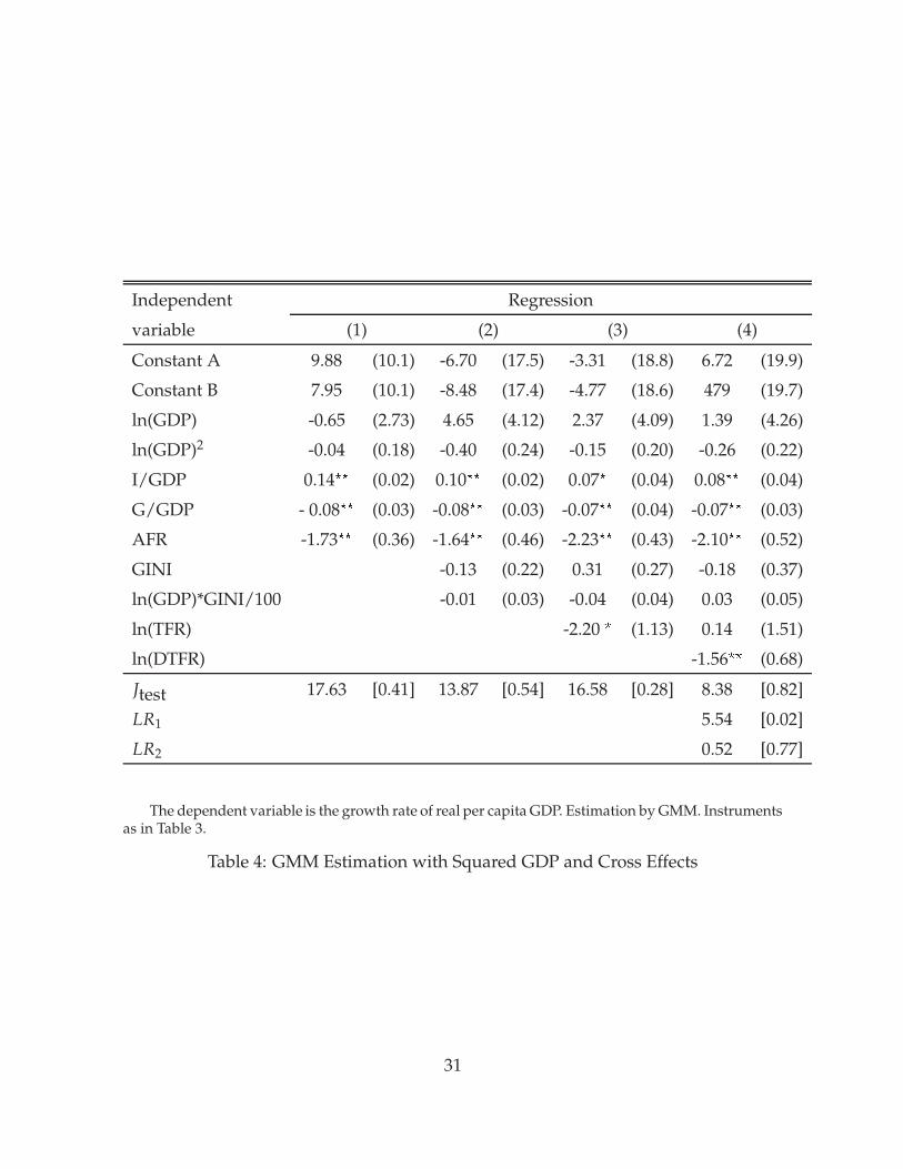
Barro (2000) argues that there are important non-linear effects that relate the levels ofdevelopment and inequality to growth rates. He shows that unless these nonlineareffects are addressed, the effects of inequality and fertility on growth are difficult todistinguish. To check whether our findings are robust with respect to the inclusionof non-linear terms, we add a squared term for GDP per capita and an interactionterm involving GDP and inequality to the explanatory variables. Table 4 presentsthe results. The new terms are never significant and do not affect the significance

32

of the J-tests. Given our relatively small number of observations, the inclusion ofadditional variables lowers the significance of the other variables. In particular, theGini coefficient is now never significant, but total fertility is significant in regression(3). Our main conclusion remains: when differential fertility is added in regression(4), it is significant, while total fertility is not. Differential fertility again improves thevalue of the J-test.13

In summary, we find that standard growth regressions detect the effect of differentialfertility on growth postulated by our model. The effects implied by the regressionsare sizable. At the same time, including differential fertility leaves the direct effect ofthe Gini coefficient insignificant, with a positive point estimate.

6 Conclusion

Most of the theoretical literature on inequality and growth has concentrated on chan-nels where inequality affects growth through the accumulation of physical capital.In this paper we propose a different mechanism which links inequality and growththrough differential fertility and the accumulation of human capital. In our model,families with less human capital decide to have more children and invest less in edu-cation. When income inequality is high, large fertility differentials lower the growthrate of average human capital, since poor families who invest little in education makeup a large fraction of the population in the next generation. A calibration exerciseshows that these effects can be fairly large. In the benchmark case, raising the Ginifrom 0.2 to 0.65 lowers the initial annual growth rate by 1.4%. We also examine therole of differential fertility in the growth-regression framework used, among others,by Perotti (1996) and Barro (2000). In line with the predictions of the theory, we findsizable negative effects of differential fertility on growth. Both the empirical resultsand the quantitative analysis of the model suggest that the differential-fertility chan-nel is important for accounting for the cross-sectional relationship between inequalityand growth.

13As an additional test of the robustness of our results, we also carried out regressions with initial lifeexpectancy as an explanatory variable. Growth regressions generally show life expectancy to be moreclosely related to growth than other demographic variables such as the total fertility rate. However,even if we add life expectancy to regression (4) in Table 3, differential fertility continues to have asignificantly negative effect on growth, albeit with a lower point estimate of -0.79.

33

We also examine the time series implications of our model for the joint evolution ofinequality, fertility, and growth. Since in our overlapping-generations model a pe-riod is one generation, the dynamics of the model are to be interpreted as changeswhich occur over a horizon of a century or more. Here we find that the model is ableto explain key features of the evolution of income, fertility, and inequality in indus-trializing countries in the last 200 years. Specifically, the model generates an initialincrease and ultimate decline in inequality and fertility. The same pattern has beenobserved in many industrializing countries in the 19th and early 20th centuries. Inaddition, if we specify the model to allow for endogenous growth, the model gen-erates steadily increasing growth rates throughout the transition, which is anotherstylized feature of the data.

Our analysis provides a new perspective on the link between economic growth andpopulation growth. Existing studies have found little correlation between the growthrates of population and output per capita (see Kelley and Schmidt 1999), which hasled some researchers to conclude that population does not matter for growth. Theresults in this paper suggest that it is not overall population growth, but the distri-bution of fertility within the population which is important. In other words, who ishaving the children matters more than how many children there are overall.

A natural direction for further research concerns the policy implications of our model.Since differential fertility rather than inequality per se is the main source of growtheffects, it is not clear that redistributional policies would increase economic growth.Indeed, a typical outcome in models with endogenous fertility is that income redistri-bution tends to increase fertility differentials (see Knowles 1999), which would lowerthe growth rate. Here the policy implications of our model are in stark contrast toother theories linking inequality and growth. Compared to income redistribution,policies aimed at equalizing access to education would be more effective.

34

References

Acemoglu, Daron and Joshua D. Angrist. 2000. “How Large are Human Capital Ex-ternalities? Evidence from Compulsory Schooling Laws.” NBER MacroeconomicsAnnual 2000, pp. 9–59.

Althaus, Paul G. 1980. “Differential Fertility and Economic Growth.” Zeitschrift furdie gesamte Staatswissenschaft 136:309–326.

Angrist, Joshua D. and Alan B. Krueger. 1991. “Does Compulsory School Atten-dance Affect Schooling and Earnings?” The Quarterly Journal of Economics 106 (4):979–1014.

Ashenfelter, Orley and Alan B. Krueger. 1994. “Estimates of the Economic Return toSchooling from a New Sample of Twins.” American Economic Review 84:1157–73.

Barro, Robert J. 2000. “Inequality and Growth in a Panel of Countries.” Journal ofEconomic Growth 5:5–32.

Becker, Gary S. and Robert J. Barro. 1988. “A Reformulation of the Economic Theoryof Fertility.” Quarterly Journal of Economics 103:1–25.

Benabou, Roland. 1996. “Inequality and Growth.” NBER Macroeconomics Annual,pp. 11–74.

Boucekkine, Raouf, David de la Croix, and Omar Licandro. 2002. “Vintage HumanCapital, Demographic Trends, and Endogenous Growth.” Journal of EconomicTheory 104 (2): 340–75.

Card, David and Alan B. Krueger. 1996. “School Resources and Student Outcomes:An Overview of the Literature and New Evidence from North and South Car-olina.” Journal of Economic Perspectives 10 (4): 31–50.

Chesnais, Jean Claude. 1992. The Demographic Transition. Oxford: Oxford UniversityPress.

Dahan, Momi and Daniel Tsiddon. 1998. “Demographic Transition, Income Distri-bution, and Economic Growth.” Journal of Economic Growth 3 (March): 29–52.

Deininger, Klaus and Lyn Squire. 1996. “Measuring Income Inequality: A NewDatabase.” Development Discussion Paper No. 537, Harvard Institute for Inter-national Development.

35

Doepke, Matthias. 2001. “Accounting for Fertility Decline During the Transition toGrowth.” Working Paper No. 804, UCLA Department of Economics.

Gallant, Donald. 1987. Nonlinear Statistical Models. John Wiley & Sons.

Galor, Oded and David N. Weil. 2000. “Population, Technology, and Growth: FromMalthusian Stagnation to the Demographic Transition and Beyond.” AmericanEconomic Review 90 (4): 806–28.

Galor, Oded and Hyoungsoo Zang. 1997. “Fertility, Income Distribution, and Eco-nomic Growth: Theory and Cross-Country Evidence.” Japan and the World Econ-omy 9:197–229.

Glomm, Gerhard and B. Ravikumar. 1992. “Public Versus Private Investment inHuman Capital: Endogenous Growth and Income Inequality.” Journal of PoliticalEconomy 100 (4): 818–834.

Hansen, Lars P. 1982. “Large sample properties of generalized method of momentsestimators.” Econometrica 50:1029–1054.

Hansen, Gary D. and Edward C. Prescott. 1999. “Malthus to Solow.” Federal Re-serve Bank of Minneapolis Staff Report 257.

Haveman, Robert and Barbara Wolfe. 1995. “The Determinants of Children’s At-tainments: A Review of Methods and Findings.” Journal of Economic Literature33:1829–78.

Jazairy, Idriss, Mohiuddin Alamgir, and Theresa Panuccio. 1992. The State of WorldRural Poverty: An Inquiry Into Its Causes and Consequences. New York: New YorkUniversity Press.

Jones, Elise F. 1982. Socio-Economic Differentials in Achieved Fertility. World Fertil-ity Survey Comparative Studies No. 21. Voorburg, Netherlands: InternationalStatistics Institute.

Kelley, Allen C. and Robert M. Schmidt. 1999. “Economic and Demographic Change:A Synthesis of Models, Findings, and Perspectives.” Duke University Depart-ment of Economics Working Paper No. 99/01.

Knowles, John. 1999. “Can Parental Decisions Explain U.S. Income Inequality?”Working Paper, University of Pennsylvania.

36

Kremer, Michael and Daniel Chen. 2000. “Income Distribution Dynamics with En-dogenous Fertility.” NBER Working Paper 7530.

Krueger, Alan B. and Mikael Lindahl. 2001. “Education and Growth: Why and forWhom?” Journal of Economic Literature 39 (1): 1101–36.

Leibowitz, Arleen. 1974. “Home Investments in Children.” Journal of Political Econ-omy 82:S111–S131.

Maddison, Angus. 2001. The World Economy: A Millennial Perspective. Paris: OECD.

Mboup, Gora and Tulshi Saha. 1998. Fertility Levels, Trends, and Differentials. Demo-graphic and Health Surveys Comparative Studies No. 28. Calverton, Md: MacroInternational.

Morand, Olivier F. 1999. “Endogenous Fertility, Income Distribution, and Growth.”Journal of Economic Growth 4:331–349.

Perotti, Roberto. 1996. “Growth, Income Distribution, and Democracy: What theData Say.” Journal of Economic Growth 1 (2): 149–87.

Psacharopoulos, George. 1994. “Returns to Investment in Education: A GlobalUpdate.” World Development 22 (9): 1325–43.

Rangazas, Peter. 2000. “Schooling and Economic Growth: A King-Rebelo Experi-ment with Human Capital.” Journal of Monetary Economics 46:397–416.

Rosenzweig, Mark R. and Kenneth I. Wolpin. 1994. “Are There Increasing Returns tothe Intergenerational Production of Human Capital.” Journal of Human Resources29:670–93.

Sachs, Jeffrey and Andrew Warner. 1997. “Fundamental Sources of Long-RunGrowth.” American Economic Review Papers and Proceedings 87:184–188.

United Nations. 1987. Fertility Behaviour in the Context of Development: Evidence fromthe World Fertility Survey. Population Studies No. 100. New York: United Nations.

. 1995. Women’s Education and Fertility Behavior. New York: United Nations.

Wiggins, Stephen. 1990. Introduction to Applied Nonlinear Dynamic Systems and Chaos.Springer-Verlag.

Williamson, Jeffrey G. 1985. Did British Capitalism Breed Inequality? Boston: Allenand Unwin.

37

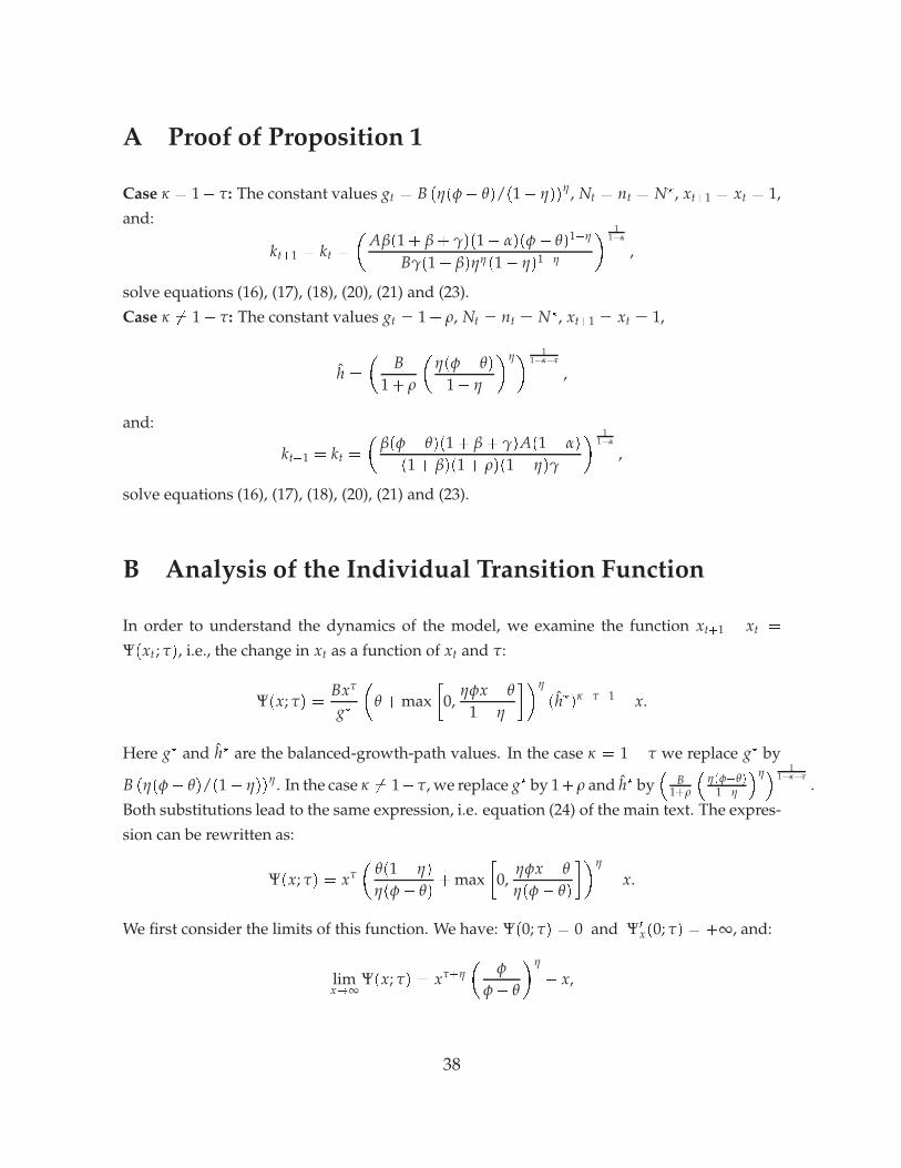
A Proof of Proposition 1

Case κ = 1� τ: The constant values gt = B (η(φ� θ)/(1� η))η, Nt = nt = N?, xt+1 = xt = 1,

and:

kt+1 = kt =

�Aβ(1 + β + γ)(1� α)(φ� θ)1�η

Bγ(1+ β)ηη(1� η)1�η

� 11�α

,

solve equations (16), (17), (18), (20), (21) and (23).

Case κ 6= 1� τ: The constant values gt = 1+ ρ, Nt = nt = N?, xt+1 = xt = 1,

h =

�B

1+ ρ

�η(φ � θ)

1� η

�η� 11�κ�τ

,

and:

kt+1 = kt =

�β(φ � θ)(1 + β + γ)A(1� α)

(1 + β)(1 + ρ)(1� η)γ

� 11�α

,

solve equations (16), (17), (18), (20), (21) and (23).

B Analysis of the Individual Transition Function

In order to understand the dynamics of the model, we examine the function xt+1 � xt =

Ψ(xt ; τ), i.e., the change in xt as a function of xt and τ:

Ψ(x; τ) =Bxτ

g?

�θ +max

�0,

ηφx� θ

1� η

��η

(h?)

κ+τ�1� x.

Here g? and h? are the balanced-growth-path values. In the case κ = 1� τ we replace g? by

B (η(φ� θ)/(1� η))η. In the case κ 6= 1� τ, we replace g? by 1+ ρ and h? by�

B1+ρ

�η(φ�θ)

1�η

�η� 11�κ�τ

.

Both substitutions lead to the same expression, i.e. equation (24) of the main text. The expres-

sion can be rewritten as:

Ψ(x; τ) = xτ

�θ(1� η)

η(φ� θ)+ max

�0,

ηφx� θ

η(φ � θ)

��η

� x.

We first consider the limits of this function. We have: Ψ(0; τ) = 0 and Ψ0

x(0; τ) = +∞, and:

limx!∞

Ψ(x; τ) = xτ+η

�φ

φ� θ

�η

� x,

38

which implies:

limx!∞

Ψ(x; τ) = �∞ if τ + η < 1 and limx!∞

Ψ(x; τ) = +∞ otherwise.

Hence the function Ψ starts from (0, 0) with an infinite slope and goes either to �∞ or +∞

depending on parameter values.

By definition of the aggregate balanced growth path, x = 1 is a steady state and thus Ψ(1; τ) =

0. This steady state is locally stable if and only if Ψ0

x(1; τ) < 0, i.e.:

τ +ηφ

φ� θ� 1 < 0.

At the point:

τ = 1�ηφ

φ� θ

the dynamics of individual capital described by: xt+1 � xt = Ψ(xt ; τ) undergo a transcritical

bifurcation, as proved in Proposition 2. There are thus two steady-state equilibria, 1 and x,

near (1, τ) for each value of τ smaller or larger than τ. The equilibrium 1 (resp. x) is stable

(resp. unstable) for τ < τ and unstable (resp. stable) for τ > τ.

Another point of interest is xt =θ

ηφ . If, at this point, the function Ψ is negative, it crosses the

horizontal axes between 0 and θηφ . The existence of this steady state results from the infinite

slope of Ψ at 0 and from its continuity; uniqueness results from the concavity of the function

in the interval (0, θηφ ). We evaluate:

Ψ�

θ

ηφ, τ

�=

�θ(1� η)

η(φ� θ)

�η

�θ

ηφ

�τ

�

θ

ηφ.

This is negative if τ is above a threshold τ:

τ =(1� η) ln(θ/η) � ln φ� η ln((1� η)/(φ � θ))

ln θ � ln(ηφ).

We are now able to fully characterize the dynamics of x as a function of the parameter τ. The

bifurcation diagram is presented in Figure 2.

39