Industry Recommendations: Characteristics,

Investment Value, and Relation to Firm

Recommendations*

Ohad Kadan, Leonardo Madureira, Rong Wang, and Tzachi Zach**

September 2009

Abstract

In addition to firm recommendations, brokers also issue recommendations for industries. We study these recommendations using data newly available from IBES. First, we find that the distribution of industry recommendations is quite balanced. Brokers tend to issue optimistic recommendations to industries that show high levels of R&D intensity, past profitability and past returns, as well as to industries in which they are active in providing underwriting services. Second, industry recommendations appear to have investment value: portfolios long in industries about which analysts are optimistic and short in industries about which analysts are pessimistic generate significant abnormal returns. Finally, we find that industry recommendations contain information that is orthogonal to that included in firm recommendations. This evidence sheds new light on the interpretation and investment value of firm recommendations. It suggests that analysts typically benchmark their firm recommendations to industry peers, even when they proclaim to be using a market benchmark. In line with this view, we show that the investment value of analysts’ recommendations is enhanced when both industry and firm recommendations are used jointly.

* An earlier version of this paper was circulated under the title “Do Industry Recommendations Have Investment Value.” ** Ohad Kadan (kadan@wustl.edu) is at the Olin Business School, Washington University in St. Louis; Leonardo Madureira (leonardo.madureira@case.edu) is at the Weatherhead School of Management, Case Western Reserve University; Rong Wang (rongwang@smu.edu.sg) is at the Lee Kong Chian School of Business, Singapore Management University; and Tzachi Zach (zach_7@fisher.osu.edu) is at the Fisher College of Business, Ohio State University. We thank Alon Brav, Judson Caskey, Lauren Cohen, Doug Foster, Reuven Lehavy, Roni Michaely, Brian Richter, Ajai Singh, Brett Trueman, and seminar participants at Case Western Reserve University, Ohio State University, UCLA, and Washington University in St. Louis, as well as participants at the IDC Summer Conference 2009, SMU Summer Camp 2009, and the 2009 Asian Finance Association Meeting.

1

1 Introduction

Analysts’ industry knowledge is highly valued by investors. For example,

Institutional Investor Magazine has been surveying institutional investors on the

importance of various attributes in sell-side research analysts. For the past 11 years

(1998-2008), industry knowledge was deemed the most important research attribute of

equity analysts.1 Indeed, sell-side analysts are industry specialists. They are typically

hired to and work in industry groups, each group covering a set of firms that are similar

to each other in their industry characteristics. Analysts then publish information both at

the industry and firm levels. At the industry level, they write periodic industry reports,

provide forecasts for the industry and offer industry recommendations. At the firm level,

they analyze specific firms in their assigned industry, providing earnings estimates,

recommendations, price targets, etc. The extant literature has explored analysts’ stock

recommendations extensively.2 Despite their prominence, the literature has not studied

industry recommendations, probably due to the lack of large scale data. In this paper we

attempt to fill this gap.

To motivate the analysis, consider the following example. During the second half

of 2007, the median stock recommendation issued for both GM and Chevron was a

‘hold.’ However, at that time, analysts issued bearish recommendations for the

Automobiles industry as a whole, while they typically issued bullish recommendations

for the Oil industry. This scenario raises several interesting questions.

First, what are the industry attributes that determine industry coverage and the

level of industry recommendations? In the example above, one might ask whether

analysts favored the energy industry because it had shown high past returns, high

profitability, or perhaps high equity issuance volume. Second, do recommendations for

industries have any value to investors? After all, these recommendations are likely based

on public and often stale information. Indeed, during the time period of the example

above, it was common knowledge that oil prices were sky-rocketing, benefiting the oil 1 See: http://www.iimagazine.com/Rankings/RankingsEqtyTeamAmerica08.aspx?src=http://www.iimagazinerankings.com/rankingsEqtyTeamAmerica08/whatInvestorsWant.asp . 2 For a recent review of the literature see Ramnath, Rock, and Shane (2008).

2

producers while hurting automobile manufacturers. Third, to the extent that industry

recommendations do convey information, is this information incremental to that already

included in firm recommendations? In the example above, investors ought to know

whether to interpret the ‘hold’ recommendation associated with GM and with Chevron

identically or whether they should take into account the different industry

recommendations. More generally, industry recommendations may be just aggregations

of firm specific recommendations. Alternatively, they may include information that is

orthogonal to firm recommendations – and thus can be used to enhance the performance

of investment strategies based on firm recommendations. Finally, what can we learn

about firm recommendations from comparing them with industry recommendations? In

particular, do analysts benchmark their firm recommendations to the market or to

industry peers? In the example above, when analysts issued a ‘hold’ recommendation to

GM it is important to understand whether this signal was relative to the entire market or,

instead, relative to peers such as Ford, Chrysler, and Toyota.

To answer these questions we use the IBES database to collect industry

recommendations. When an analyst produces a report with a recommendation on a firm’s

stock, she often includes in the report her current outlook on that firm’s industry. In

September 2002, IBES started recording the textual information on the industry outlook

for those brokers reporting the industry recommendation in their firm reports. This

information is recorded in the detailed stock recommendation file. Similar to firm

recommendations, the text of the industry recommendations is either optimistic (such as

‘overweight’), neutral (such as ‘equal weight’), or pessimistic (such as ‘underweight’).

Since industry recommendations are attached in IBES to specific firms, we have

to adopt a particular mapping between firms and the industries to which they belong. We

follow Boni and Womack (2006) and Bhojraj, Lee, and Oler (2003), and use the Global

Industry Classification Standard (GICS), which is widely used by brokerage houses. This

enables our research design to closely mirror the intentions of the broker when issuing the

industry recommendation.

Our sample uses six major financial institutions for which textual information on

industry outlooks is available. It includes a total of 29,184 industry recommendations in

3

the period from September 2002 through December 2007. We find that industry coverage

is pretty comprehensive with little variation in coverage across brokers and time. Thus,

unlike in the case of firm recommendations, selection bias [McNichols and O’Brien

(1997)] does not seem to be a major issue with industry recommendations.

Unconditionally, 30% of the industry recommendations are optimistic, 55% are neutral,

and 15% are pessimistic. We study the factors associated with the level of optimism in

industry recommendations. We find that past profitability, past returns, and the extent of

R&D activity are positively associated with the probability of issuing an optimistic

industry recommendation. Furthermore, we find some evidence that brokers are inclined

to issue an optimistic recommendation for industries in which they are active in providing

equity underwriting services. This is similar to findings related to firm recommendations

[e.g. Lin and McNichols (1998); Michaely and Womack (1999)].

We next turn to examine whether industry recommendations have value to

investors. On one hand, analysts, being industry experts, are located in a junction of

information related to the industry that they cover. They follow several companies in the

industry, talk to their executives and other analysts, and are attentive to all relevant pieces

of news. As such, they are good candidates to be the first to identify “hot” and “cold”

industries. On the other hand, several reasons conspire to make it difficult for investors to

earn abnormal returns based on industry recommendations. Some of the reasons relate to

analysts’ role in collecting and using information. The literature has covered extensively

how analysts’ expertise, special access, and relationships with the firm affect the way

analysts perform.3 Because industry analysis uses widely available information, the only

source of predictability can be a unique expertise in analyzing publicly available data.

Another issue that may limit our ability to find any predictive power in industry

recommendations is that they are likely to be quite stale when they become available on

IBES. Brokers issue industry recommendations within industry reports that they publish

on a monthly/quarterly basis. The industry recommendations that we observe are

3 For example, the presence of an underwriting relationship allows a broker to issue better earnings forecasts [Malloy (2005)] or to be a better market maker [Ellis, Michaely and O’Hara (2000); Madureira and Underwood (2008)], while the presence of a lending relationship affects the ability of a broker to secure future underwriting business [Drucker and Puri (2005); Ljungqvist, Marston, and Wilhelm (2006)], get better terms for new security offerings [Puri (1996)], or provide better earnings forecasts [Ergungor, Madureira, Nayar, and Sing (2008)].

4

recorded only when a new stock recommendation is issued. Thus, we cannot identify the

exact date in which the industry recommendation was originally issued. This and the fact

that industry recommendations are issued infrequently suggest that any trading strategy

relying on industry recommendations will be based on stale information.

We study the investment value of industry recommendations by computing risk-

adjusted returns of industry portfolios formed based on monthly consensus industry

recommendations.4 We find that a portfolio of industries about which analysts are most

optimistic carries a significant out-of-sample alpha of 0.46% per month, while a

pessimistic portfolio carries a significantly negative alpha of 1.25% per month. A hedged

portfolio long in the optimistic portfolio and short in the pessimistic portfolio yields a

significantly positive alpha of 1.3% per month.5 These are surprising results, especially

considering the admittedly simple portfolio formation methodology. Buying, and even

short-selling industry portfolios is simple and incurs low transaction costs using industry

Exchange Traded Funds (ETFs). In addition, we find that while analysts do chase

industry momentum [Moskowitz and Grinblatt (1999)], the abnormal returns from

industry recommendations is not driven by it.

We then turn to studying the relation between industry and firm

recommendations. In particular, we attempt to identify whether firm recommendations

contain information regarding industry outlooks, or whether firm recommendations just

rank firms within industries. Our first step is to examine what brokers disclose on how

their recommendations should be interpreted. By examining these disclosures for the 20

largest brokers (in terms of numbers of recommendations), we find that 10 of these

brokers (including the six in our industry recommendation sample) benchmark their firm

recommendations to industry peers, while the other ten rely on a market benchmark.

Different benchmarks imply different ways by which firm recommendations reflect

industry information.

4 Our main measure of risk-adjustment is the out-of-sample alpha obtained relative to the Fama-French four factors. This approach is similar to Brennan, Chordia, and Subrahmanyam (1998) and Chordia, Subrahmanyam, and Anshuman (2001). 5 We also compute the traditional in-sample alphas from simply running the Fama-French four factor model over the whole time series of excess returns on each portfolio. For all examinations in this paper, in-sample alphas are comparable – and even larger in terms of magnitude and significance – to the ones obtained with out-of-sample alphas.

5

If brokers use an industry benchmark for their firm recommendations then their

firm recommendations will contain no industry-wide information. Essentially such

brokers limit their firm recommendations to ranking firms within industries. By contrast,

if brokers use a market benchmark, then their firm recommendations are expected to

incorporate industry outlooks. To help us distinguish between these alternatives we

construct “pseudo industry consensus recommendations” – similar to those used in Boni

and Womack (2006) – by value weighting all firm recommendations that belong to a

specific GICS industry. Interestingly, we find that the correlation between the pseudo

industry recommendations and the true industry recommendations is low (around 0.12),

suggesting that the two are based on different information. We then repeat the abnormal

return analysis using the pseudo industry recommendations. In stark contrast to the

results with true industry recommendations, the analysis using pseudo industry

recommendations shows no abnormal returns. These results hold for the entire sample as

well as for both subgroups of brokers: those who disclose the use of industry benchmarks

and those who disclose the use of market benchmarks. Hence, it appears that true industry

recommendations contain information regarding industry outlooks which is not already

reflected in firm recommendations or in aggregations thereof. This suggests that analysts

benchmark their firm recommendations to industry peers regardless of the stated

benchmark which appears in their disclosures. This extends the findings of Boni and

Womack (2006) who concluded that analysts’ strength is in ranking firms within

industries. Furthermore, this result shows that industry recommendations contain

information which is orthogonal to that included in firm recommendations.

Prior research demonstrates that firm recommendations carry investment value.6

If indeed firm recommendations are largely aimed at ranking firms within industries, then

conditioning firm recommendations on the prospects of the relevant industry should

increase their investment value. Our next tests pursue this line of thought by combining

the information in both industry and firm recommendations in forming monthly

portfolios. At the industry level, we classify industries into three portfolios based on true

industry recommendations as before. At the firm level, we follow Boni and Womack

6 See for example Stickel (1995); Womack (1996); Barber, Lehavy, McNichols, and Trueman (2001, 2006); Jegadeesh, Kim, Krische and Lee (2004); and Barber, Lehavy, and Trueman (2008).

6

(2006) and classify firms into net upgraded and net downgraded firms. A firm can be

allocated to one of six portfolios depending on its own recommendation

(upgraded/downgraded) and the consensus recommendation for its industry (one of three

tiers).

The results support the idea that industry and firm recommendations are

complementary and that combining them adds investment value. For example, net

upgraded stocks have abnormal returns only if they are part of the industries with the best

(optimistic) outlook, but not when they are part of the industries with the worst

(pessimistic) outlook. In a similar fashion, net downgraded stocks have significantly

negative alphas only when part of a pessimistic industry. A portfolio that is long in

upgraded firms in the most optimistic industries and short in downgraded firms in the

most pessimistic industries generates a striking out-of-sample abnormal return of 2.2%

per month. Thus, investment strategies that exploit both industry and firm

recommendations appear to outperform strategies that use just one of the two.

Our paper contributes to the extant literature in several ways. To our knowledge,

this is the first paper to analyze industry recommendations, highlighting a new dimension

of information provided by financial analysts. The ability to extract abnormal returns

from a simple trading strategy based on industry recommendations shows the relevance

of these recommendations from an investment perspective and reinforces the findings of

Institutional Investor Magazine. The paper also sheds new light on the information

contained in firm recommendations. This information appears to be mostly about ranking

stocks within industries, even among brokers who proclaim not to be using industry

benchmarks. Thus, industry recommendations are very different from just an aggregation

of firm recommendations. As we show, firm recommendations are best interpreted in

conjunction with industry recommendations, jointly yielding higher investment value.

This aspect of the paper directly extends the evidence in Boni and Womack (2006) who

analyze aggregations of firm recommendations but not “true” industry recommendations.

Our paper also relates to the literature exploring the relative importance of

industry selection in the investment process. Busse and Tong (2008) report that the

industry selection component of a typical actively managed mutual fund accounts for

7

about half of that fund’s risk-adjusted return. Kacperczyk, Sialm and Zheng (2005) show

that funds that concentrate holdings in fewer industries – the ones in which they have

some informational advantages – tend to outperform the more diversified funds.

Avramov and Wermers (2006) show that optimally-chosen portfolios based on

predictable variation in mutual funds’ characteristics outperform their benchmarks, and

one important source of this outperformance is the portfolios’ strategic allocation to

specific industries over the business cycle. Our results add to this literature by directly

showing that industry specialists are capable in providing useful industry outlooks.

The rest of the paper proceeds as follows. In section 2 we describe the data. In

Section 3 we explore the characteristics of industry recommendations. In Section 4 we

study the investment value of firm recommendations. Section 5 discusses the relation

between industry and firm recommendations. Section 6 concludes.

2 Data

2.1 Brokers and Industry Recommendations

Starting in September of 2002 IBES began to record industry recommendations

made by analysts alongside firm recommendations. This information is recorded in the

‘btext’ field in the IBES recommendation file. This field always contains the text of the

firm recommendation (e.g. ‘buy’, ‘hold’, ‘underperform’). For investment banks which

include an industry recommendation in their firm reports, the field also records the

industry recommendations. See Appendix for details.

By analyzing the IBES database we find that six out of the top 20 (in terms of

number of recommendations published per year) investment banks consistently provide

industry recommendations in their firm reports during our sample period: September

2002 through December 2007.7 Table 1 lists those investment banks along with some

information regarding their coverage. As listed, the investment banks in our sample are

Bear Stearns, Credit Swiss, Goldman Sachs, Morgan Stanley, CIBC, and Lehman Bros. It

7 The IBES tapes we used were downloaded in 2008. These are free from the data problems identified in Ljungqvist, Malloy, and Marston (2009). These problems are related to IBES tapes from 2002-2004.

8

is important to note that other large investment banks (such as Merrill Lynch, JP Morgan

and others) also issue industry recommendations. However, these banks do not include

their industry recommendations in firm reports, and hence their industry

recommendations are not recorded by IBES. The six brokers in our sample account for

17% of all recommendations in IBES during our sample period. As such, they represent a

large fraction of the IBES universe.

<Insert Table 1 here>

Table 1 shows that the brokerage houses in our sample cover between 1,100 and

1,700 firms during the sample period. These brokers are active in issuing firm

recommendation: the average number of firm recommendations per month ranges from

48 to 99. They seem similar to each other along these two dimensions.

2.2 Industry Classification

IBES reports the industry recommendation issued by a broker for the industry to

which a firm belongs. However, IBES does not explicitly report the industry to which the

firm belongs, as defined by the broker. We infer this industry from the identity of the firm

and its industry classification as defined by the General Industry Classification Standard

(GICS) obtained from Compustat. This classification is maintained by Standard & Poor’s

and MSCI Barra, and is widely adopted by investment banks as an industry classification

system (as opposed to the SIC classification that is popular among academics). The GICS

system has four classification levels: 10 sectors, 24 industry groups, 69 industries, and

154 sub-industries.8 These classifications are highly intuitive, and have been shown to

better explain stock comovements compared to other popular industry classifications

[Bhojraj, Lee, and Oler (2003)]. In the context of this research, Boni and Womack (2006)

show that the GICS classification is a good proxy for how sell-side analysts specialize by

industry.9

<Insert Table 2 here> 8 Standard and Poors and MSCI Barra change their GICS industry definitions from time to time. The numbers listed here are as of the end of 2007. 9 We extend the analysis offered in Boni and Womack (2006), by comparing the analyst coverage choice in our sample relative to different industry classifications: besides GICS, we also look at SIC (2 digit), IBES internal classification and the Fama-French 48 industries. The comparison (available upon request) shows that the GICS partition most closely resembles how brokers define their industries.

9

Similar to Boni and Womack (2006) and Bhojraj, Lee, and Oler (2003), we focus

on the industry level (6 digits). Table 2 presents the complete list of industries using the

GICS classification, as well as some basic statistics of industry coverage by the six

brokers in our sample. By casually examining industry classifications in the relevant

investment banks, we find our classification to be broadly as fine as or finer than the one

used by them. This ensures that our industry classification captures variations in industry

recommendations within each broker.

2.3 Industry Recommendations

Similar to firm recommendations, brokerage houses use a variety of terms to

express optimism, neutrality, or pessimism toward industries. In the case of firm

recommendations, IBES transforms the textual recommendation into a five-point rating

system (recorded in the IRECCD item). By contrast, the text of the industry

recommendation is not recorded numerically. Hence, we convert the text using a key

presented in the Appendix. We code recommendations with an optimistic tone as ‘1’,

recommendations with a neutral tone as ‘2’, and recommendations with a pessimistic

tone as ‘3’. Thus, for each IBES entry that also includes the textual description of the

industry outlook, we have both the recommendation for the firm itself (optimistic,

neutral, or pessimistic) and the recommendation for the industry to which the firm

belongs (again, optimistic, neutral, or pessimistic).

3 Basic Characteristics of Industry Recommendations

Table 3 presents summary statistics to describe coverage and distributional

properties of industry recommendations. Panel A shows that coverage is quite

comprehensive across the universe of industries for five out of the six brokers.10 Note that

the number of GICS industries (bottom row) has increased from 59 to 69 over the years,

which seems to explain the increasing trend in coverage across brokers. We have

10 Note that during the year 2002 coverage is lower. This is because our sample period only starts in September of that year.

10

specifically examined the industries which are not covered by each broker during the

sample period. Relatively neglected industries are Water Utilities (not covered by three

out of the six brokers; see Table 2) and Tobacco (not covered by two out of the six).

Thus, it appears that unlike in stock recommendations, there is no real decision whether

to initiate or drop coverage of an industry. Rather, pretty much all the large brokers cover

almost all industries. This suggests that in contrast to firm recommendations, selection

bias [McNichols and O’Brien (1997)] is not a major issue with industry

recommendations.

<Insert Table 3 here>

Panel B presents the distribution of industry recommendations by year. The table

shows that the frequency of optimistic recommendations hovers around 30%, with very

little variation over the years. There is, however, an increase in the frequency of neutral

recommendation (from 50% to 59%) accompanied by a decrease in the proportion of

pessimistic recommendations (from 19% to 12%). Panel C presents the average industry

recommendations by broker during our sample period. The results show that there is very

little difference between the different brokers, as average recommendations hover

somewhat below ‘2’ (neutral to slightly optimistic) for all of them. These results suggest

that brokers issue a pretty balanced distribution of industry recommendations, with just a

small inclination toward optimism. In Section 5 we compare this distribution to that of

the associated firm recommendations.

To better understand the determinants of industry recommendations we examine

the probability of issuing an optimistic/pessimistic recommendation as a function of

several factors. The main explanatory variables we investigate are industry size

(aggregate market-value of all firms in the industry in the month before the

recommendation), lagged industry and market returns, and industry value-weighted

averages of market-to-book, profitability (return on assets), R&D (as a fraction of assets),

and capital expenditures (as a fraction assets). All accounting variables are measured

during the year of the recommendation. Additionally, it may be that analysts are more

optimistic about industries that have a high IPO/SEO activity in an attempt to win

underwriting business. To examine whether such conflicts of interest have an effect on

11

industry recommendations we include three variables related to equity underwriting

activity. The first two are the total and average IPO/SEO proceeds in the industry during

the year preceding the recommendation. These variables capture the volume of equity

issuance in the industry. The last variable is the percentage of IPO/SEO proceeds in an

industry underwritten by the issuing broker during the year preceding the

recommendation. This variable is close in spirit to the “affiliation” variable used in prior

research to proxy for conflicts of interest at the firm level [Lin and McNichols (1998);

Michaely and Womack (1999)]. We also control for broker fixed effects to account for

any broker-specific time invariant characteristics. We cluster the standard errors at the

broker-industry level.

Table 4 presents the results of logit models based on the explanatory variables

above. We use two specifications. In the first (second) specification the dependent

variable is a dummy equal to one when the industry recommendation is optimistic

(pessimistic) and zero otherwise.11 Consider the first specification. The probability of

issuing an optimistic recommendation is increasing in the average profitability and R&D

intensity in the industry. For example, for the median industry, a one standard deviation

increase in R&D intensity increases the probability of issuing an optimistic

recommendation by 5 percentage points.12 We also observe a momentum effect as the

probability of issuing an optimistic recommendation is increasing in the industry returns

during the three quarters preceding the recommendation. Interestingly, we also observe a

contrarian tendency relative to market returns as the coefficient on lagged market return

is negative. Finally, we observe a tendency of brokers to issue an optimistic

recommendation to industries in which they are active as underwriters: the coefficient on

the fraction of the industry’s IPO/SEO proceeds underwritten by the broker is positive

and significant.

<Insert Table 4 here>

11 Note that the two specifications are not mutually independent. They reflect the same set of results viewed from two different angles. It would have been desirable to pool the two separate logistic models into a single ordered-logit model. However, this is not possible, since the Wald test rejects the parallel regression assumption, implying that an ordered-logit (and similarly an ordered-probit) is not valid in this case. See Long and Freese (2006: p. 197-200) for details. 12 For the median firm, the marginal effect of R&D (from Table 4) is 1.16, and the standard deviation of R&D is 0.0428 (not tabulated).

12

Similar to the optimistic model, the pessimistic model shows that high R&D

activity is less likely to be associated with a pessimistic industry recommendation. Unlike

the optimistic model, we do not observe a strong momentum effect. Rather, it appears

that analysts are sluggish in incorporating negative momentum into their

recommendations as only the coefficients on the three-quarters lagged industry and

market returns are significant. Furthermore, underwriting activity does not seem to affect

the probability of issuing a pessimistic recommendation.

4 Investment Value of Industry Recommendations

There is an extensive literature showing that analysts add value with their firm

recommendations [see for example Stickel (1995); Womack (1996); Barber, Lehavy,

McNichols, and Trueman (2001, 2006); Jegadeesh, Kim, Krische and Lee (2004); and

Barber, Lehavy, and Trueman (2008)]. A natural question concerning industry

recommendations is whether they also have value from an investment perspective.

On one hand, analysts are industry experts. They are located in a cross-road of

information related to the industry that they cover. As such, they may be able to be the

first to identify “hot” and “cold” industries, and their industry recommendations may

reflect that. On the other hand, some prominent features of industry recommendations

make their investment value less obvious. First, industry recommendations are likely

based on a synthesis of macroeconomic data and aggregated firm specific data.

Generating such recommendations requires skill and experience, but it is likely that they

are based on information that is available to all. Second, industry recommendations are

issued infrequently. Typically, analysts update their industry reports on a monthly or

quarterly basis. Moreover, unlike with firm recommendations, our data does not allow us

to identify the exact date in which the industry recommendation is issued. Rather, we can

only identify whether a broker changed its industry recommendation within a month.13

13 Additionally, while the GICS system is likely to be a reasonable representation of the industry classification used by different analysts, it is not a perfect representation. Rather, different analysts use somewhat different industry classification. This introduces noise into our measurement of industry recommendations, and is likely to lower our ability to identify any value in industry recommendations.

13

Thus, any trading strategy relying on industry recommendations will necessarily involve

trading based on stale information.

The analysis in this section explores whether industry recommendations have

investment value. We analyze the returns of portfolios constructed based on the signals

conveyed by these recommendations. That is, we ask whether an investor would have

obtained abnormal returns, had she followed up on the recommendations by investing in

these portfolios. This is the common approach used to test for information in firm

recommendations [e.g., Barber, Lehavy, McNichols, and Trueman (2001, 2006), Boni

and Womack (2006), and Barber, Lehavy, and Trueman (2008)].14

4.1 Recommendation Portfolios

We first aggregate the recommendations to create consensus industry

recommendations. This is likely to average away idiosyncratic views of individual

brokers. We compute a consensus recommendation for each one of the GICS industries

and each month during our sample period by averaging all the industry recommendations

issued during that month by all the brokers in our sample. For example, if brokers issued

10 recommendations for firms in the Media industry in month t, then the consensus

recommendations for the Media industry would be the average of the industry

recommendations recorded from the ‘btext’ field in those 10 recommendations.

This approach allows us to capture changes in industry recommendations during a

month. For example, if a broker changed her recommendation for the Media industry

from ‘1’ to ‘2’ during the month, then the consensus for month t will be affected by this

change. This approach is also robust to cases in which brokers use an industry

classification system which is somewhat different than GICS. For example, suppose that

a broker covers the ‘Utilities’ industry, but does not distinguish between the GICS

classification of ‘Gas’ and ‘Electric Utilities’. Then, our averaging approach ensures that

the industry recommendation we record will be identical for ‘Gas’ and ‘Electric utilities’.

14 Another common approach involves looking at investors’ short-term reactions to newly issued recommendations. However, since this approach depends on knowing the exact recommendations’ issuance day, it cannot be applied here.

14

Thus, while our classification may be finer than the one used by the broker, the industry

recommendation we calculate does capture the broker recommendation as intended.

Next, in each month t of our sample period, we construct three industry portfolios

based on the consensus recommendations in month t-1 as follows: Portfolio 1 in month t

includes industries with consensus industry recommendation in month t-1 less than or

equal 1.5; Portfolio 2 includes industries with consensus industry recommendation

between 1.5 and 2.5; and Portfolio 3 includes industries with consensus recommendation

greater than 2.5. Hence, Portfolio 1 in month t contains the industries about which

analysts were most optimistic in month t-1, while Portfolio 3 contains the industries about

which analysts were most pessimistic. In this aggregation, we omit industries that are not

covered by at least three brokers in a given month. We do this to ensure that the

consensus indeed aggregates information across brokers, and does not represent the

idiosyncratic view of just one or two brokers.

<Insert Table 5 here>

Panel A of Table 5 presents summary statistics related to the three portfolios and

the portfolio formation procedure. First, note that Portfolios 1 and 2 are well defined in

all 64 months of our sample period. By contrast, Portfolio 3 (the pessimistic portfolio) is

only defined in 46 months. Thus, there are 18 months in which there aren’t at least 3

analysts who collectively are pessimistic about even one industry. The average number of

industries falling in Portfolios 1 through 3 in a given month is 6.3, 20.1, and 2.2,

respectively.

Note that an alternative approach would be to assign industries to portfolios based

on a certain percentile (such as deciles). This approach is common in the momentum and

over-reaction literature. However, the literature on analysts has typically avoided this

type of arbitrary sorting, which ignores the literal meaning of the recommendations. For

example, Panel A of Table 5 shows that if we were to always allocate the lowest decile of

consensus recommendations into a pessimistic portfolio we would occasionally treat

industries as having a negative outlook despite the fact that analysts assign these

industries a neutral outlook. An investment strategy based on such an arbitrary sort would

miss the correct interpretation of the analysts’ recommendation.

15

Panel A of Table 5 reveals two additional important facts. First, the turnover in

the industry portfolios is quite high. An industry resides in any of the portfolios for an

average period of about 1-2 months. Thus, while brokers seem to change their views on

industries relatively infrequently,15 the consensus and the structure of the portfolios

change often. Second, the different industries are quite evenly distributed among the three

portfolios. Over our sample period 50 out of the 69 industries belonged to Portfolio 1 at

some point. Portfolio 3 is the least represented, but still around half of the industries

belonged to this portfolio at some point. Both these results suggest that the classification

to the three portfolios is not degenerate, and can potentially contain information.

4.2 Raw Returns

Using CRSP data we calculate a monthly return for each one of the three

portfolios in two steps. First, we calculate a month t industry return for each one of the

GICS industries. This is the value-weighted return across all CRSP firms in the relevant

industry, where the weights are based on market values at the end of month t-1.16,17

Second, we calculate the monthly return for portfolios 1-3 as the equal weighted return of

all industries in the relevant portfolio.

Panel B of Table 5 reports raw monthly returns related to different time periods

for each one of the three portfolios. To interpret the results, recall that portfolios in month

t are formed based on consensus industry recommendations in month t-1. Consider first

the average returns in month t-1. It is monotonically decreasing as we move from

Portfolio 1 (1.7%) to Portfolio 3 (0.9%, insignificant). A similar trend is observed also in

15 We can proxy for the frequency of issuance of industry recommendations by looking at the number of days between changes in the industry recommendations. Using the series of recommendations issued by an analyst to a firm we find all instances when the newly reported industry recommendation differs from the previously reported recommendation; for each such instance we define age as the number of days since the previous level of industry recommendation was first reported. The mean (median) age of those instances, across all pairs of analysts and stocks, is about 320 (217) days in our sample. 16 The most obvious and least costly way to “buy” or “sell” an industry is to buy or sell the appropriate industry ETF. By calculating the industry return as a weighted average of all CRSP firms in this industry we essentially replicate the return on the corresponding industry ETF. 17 If a firm is delisted at time t, its monthly return plus its delisting return from CRSP are used in the computation of its industry return. If a firm has a missing return at time t, we exclude it from the computation of the industry return. In a robustness test we replace the return of a firm with a missing return in month t by the market return during that month; results are not sensitive to this change.

16

month t-2. Consistent with the logit results, these trends suggest that analysts chase

industry momentum. Consider now the returns in month t. These reflect the returns to

portfolios constructed based on the industry recommendations issued in the previous

month. The monthly return on Portfolio 1 is 1.6% which is significantly different from

Portfolio 3’s return of -0.2%. Moreover, a hedged portfolio long in Portfolio 1 and short

in Portfolio 3, during the 46 months in which Portfolio 3 exists, yields a significant 1.5%

per month.

When examining the returns of the different portfolios starting from month t+1,

we do not find a significant difference between the three portfolios. This is consistent

with the high turnover of industries in our portfolios. Recall from Panel A that industries

reside in the pessimistic portfolio for a period of about one month, indicating that the

pessimistic outlook implied by the industry recommendations in month t-1 does not

persist beyond month t. These preliminary examinations suggest that if there is any kind

of predictive power in the industry recommendation, it is concentrated in a relatively

short time horizon of one month.

4.3 Risk-Adjusted Returns

We next turn to evaluating whether portfolios based on industry recommendations

can generate abnormal returns. We estimate out-of-sample alphas of the four industry

portfolios relative to the Fama-French four factors (excess market return, HML, SMB,

and UMD). Our approach is similar to Brennan, Chordia, and Subrahmanyam (1998) and

Chordia, Subrahmanyam, and Anshuman (2001). For each month t in our sample period,

we regress the monthly excess returns of the three industry portfolios on the returns of the

Fama-French four factors during the preceding 60 months: t–60 to t–1. Thus, for each

month t in our sample period we obtain an estimate of the four-factor loadings as of that

month. Denote these factor loadings by , ,MKT p t , , ,SMB p t , , ,HML p t , and , ,UMD p t , where,

for example, , ,MKT p t stands for the loading on the market factor related to month t and

portfolio p (where p=1,..,3 is one of the three industry portfolios).

17

Now, for each month t we calculate the out-of-sample four-factor alpha of

portfolio p (denoted ,p tAlpha ) as the realized excess return of the portfolio less the

expected excess return calculated from the realized returns on the factors and the

estimated factor loadings:

, , , , , , ,

, , , , ,

p t p t t MKT p t MKT t t SMB p t t

HML p t m UMD p t t

Alpha RET Rf RET Rf SMB

HML UMD

where ,p tRET , ,MKT tRET , and tRf are the realized returns on industry portfolio p, the

CRSP value-weighted index, and the risk-free rate, respectively, during month t; and

RETMKT,t-Rft, SMBt, HMLt, and UMDt are the appropriate realized returns on the factor

portfolios in month t.

For each of the three portfolios we thus obtain a time series of 64 (46 for p=3)

out-of-sample alpha estimates as well as a time series of factor loadings. Panel A of Table

6 reports the averages of these estimates. The average out-of-sample alpha of portfolio 1

is 0.46% per month (5.5% per year), significant at the 5% level. Portfolio 2 does not

show an abnormal return. By contrast, portfolio 3 generates a negative alpha of 1.25%

per month. Finally, a hedged portfolio long in portfolio 1 and short in portfolio 3 yields a

significant average out-of-sample alpha of 1.3% per month. To annualize this number

note that the hedged portfolio can only be held about 8 months in each year because

portfolio 3 only exists about 70% of the time. Hence an estimate of the annualized

abnormal return of the hedged portfolio is 1.3%*8=10.4% (assuming that whenever

portfolio 3 does not exist, the investment strategy has zero alpha).18

<Insert Table 6 here>

For completeness and to facilitate comparison with other studies we also

conducted an in-sample analysis in which we regress the excess return of the different

portfolios on the four Fama-French factors as in Barber, Lehavy, McNichols, and Truman

(2001, 2006). The intercept from this regression is an estimate of the in-sample alpha.

18 In practice trading in industries can be done using industry/or sector ETFs. The trading costs associated with such instruments are very low. The bid-ask spreads are about 0.05%, the annual management fees are around 0.5%, and the price impact is negligible. Overall, our calculations suggest that transaction costs knock-off around 1% of value per year, which is about 10% of the alpha of these trading strategies.

18

The results from this analysis are reported in Panel B of Table 6. They are comparable

(and even larger) in magnitude and statistical significance to the out-of-sample results.

For example, the in-sample alpha of the hedged portfolio is a significant 1.7% per month

(13.6% annually based on eight trading months in a year).19

Table 6 also reports the factor loadings of the portfolios. It is interesting to note

that the hedged portfolio has a small yet positive and significant (p-value of 5.7%) market

exposure in the out-of-sample analysis (beta of 0.12 in Panel A). The beta is not different

from zero in the in-sample regression (Panel B). Both the in-sample and out-of-sample

results show that the hedged portfolio loads negatively on the HML factor and positively

on the UMD factor – with the loadings on the individual industry portfolios showing that

this is mostly due to pessimistic industries relying more on growth stocks and less on

momentum.

The predictive value of industry recommendations may seem surprising,

particularly given that our portfolios are formed based on industry recommendations that

are potentially stale. Indeed, the portfolios are formed only at the end of each month, and,

second, they are based on industry consensus recommendations rather than on changes in

the industry consensus. In the context of firm recommendations, for example, Jegadeesh,

Kim, Krische and Lee (2004) show that their value is more robustly extracted from

changes in the consensus. Notice, however, that the results in Table 5 show that the

turnover of industries in our portfolios is quite high. For example, the average number of

months an industry with pessimistic outlook remains in Portfolio 3 is only 1.19 months

after its inclusion in the portfolio. That is, while our methodology of portfolio formation

formally relies on consensus industry recommendations, it creates portfolios that, in

practice, are very close to being based on changes in such consensus.20,21

19 In-sample alphas are also computed for the examinations in the next sections, and they confirm and even magnify the results obtained with out-of-sample alphas. For brevity, we do not report these in-sample alphas. They are available upon request. 20 In fact, if we update the portfolio formation procedure to force the turnover to be exactly 1 month – that is, each industry remains exactly one month after inclusion in the portfolio, the results (available upon request) become even stronger. For example, forcing away staleness brings the out-of-sample alpha of Portfolio 1 from 0.4% to 0.9% (p-value from 0.048 to 0.0006), and the out-of-sample alpha of Portfolio 3 from -1.2% to -1.5% (p-value from 0.02 to 0.008). We prefer to keep our more simplified procedure as a more conservative method to test the profitability of the industry recommendations.

19

Another effect of our methodology of portfolio formation is to mix together views

from different analysts. Given that our industry classification does not match exactly the

one used by the analyst, the averaging of individual views has the potential benefit of

reducing the noise in our classification scheme. In fact, the risk-adjusted returns, for the

most part, vanish when we define portfolios based on the recommendations of a single

broker. That is, our results suggest that sell-side analysts collectively are able to identify

winners and losers among industries. It is important to note, however, that much of the

predictability that we indentify comes from short selling a small group of industries that

are in Portfolio 3 (see Panel A of Table 5). The difference between the abnormal returns

in Portfolios 1 and 2 (which together account for more than 90% of the industries) is not

statistically significant.

As we have noted before, analysts chase industry momentum in their industry

recommendations. Industry momentum is also known to generate abnormal returns

[Moskowitz and Grinblatt (1999)]. Thus, it is interesting to ask whether the abnormal

returns related to industry recommendations are attributed to industry momentum. To

answer this question we constructed industry momentum portfolios and compared their

returns to the industry recommendations portfolios. The results of this analysis

(unreported for brevity) indicate that there is no significant industry momentum in our

sample. Furthermore, the abnormal returns related to industry recommendations are

significantly higher (both statistically and economically) than those related to industry

momentum.22

21 We can also relax the rule of forming portfolio at the end of the month by allowing industries to enter or exit a portfolio at any day. For example, we can use the consensus from the last 30 days to decide what to do with an industry – e.g., if the consensus is below 1.5, the industry enters the optimistic industry portfolio at the end of the day, and is kept in the portfolio as long as the 30-days rolling consensus remains below 1.5. We can then create portfolio daily returns and run in-sample and out-of-sample procedures using daily data. The results (available upon request) are qualitatively similar to those we report throughout the paper. 22 A remarkable aspect of our results is that analysts are able to provide abnormal returns by choosing assets among a very small set of candidates, even as each such asset is unlikely to provide abnormal performance on its own. According to Moskowitz and Grinblatt (1999), there is little evidence “that unconditional abnormal industry returns exist per se,” and we confirm in our sample that less than 10% of the individual GICS carry significant out-of-sample alphas over our sample period.

20

5 Relation between Industry and Firm Recommendations

Typically, the same analysts in investment banks issue both industry and firm

recommendations. In this section we explore to what extent the two types of

recommendations are related, whether they reflect distinct pieces of information, and

whether they can be jointly used to enhance the investment value of analysts’

recommendations.

5.1 Preliminary Analysis

It seems reasonable that industry and firm recommendations are at least somewhat

related. For example, an analyst can employ a top-down approach under which she

collects and analyzes macroeconomic data, demand and supply information for the

industry, etc. This analysis influences her understanding of the prospects of each firm in

the industry. From a bottom-up perspective, an analyst can study many firms in the

industry and then extract common aspects that help her understand the prospects of the

industry as a whole. Both approaches suggest that the outlooks expressed at the industry

and firm levels should be related. On the other hand, relatedness does not imply perfect

alignment between recommendations at the industry and firm levels. In fact, one can

view a firm’s prospects as driven by two components, one linked to its industry’s overall

prospects and the other associated with the firm’s idiosyncratic characteristics – allowing,

for example, for existence of winners and losers in the same industry. Therefore, we

expect the outlooks expressed at the industry and firm levels to be related, but only to a

certain degree.

<Insert Table 7 here>

Table 7 provides a preliminary look at the interaction between industry and firm

recommendations. The table reveals a significant variation in firm recommendations

within each level of industry recommendation. For example, out of the firm

recommendations issued with an optimistic industry recommendation, 39% are rated

optimistic, 48% are rated neutral, and 13% are rated pessimistic. We also see a wide

dispersion of firm recommendations issued with neutral and pessimistic industry

recommendation. The average firm recommendation for firms in industries rated as

optimistic is 2.73, in industries rated neutral is 2.79, and in industries rated pessimistic is

21

2.9 – and the differences between these numbers are significant. This shows that there is

a positive correlation between industry and firm recommendations. That is, analysts are

more likely to issue an optimistic recommendation for firms belonging to industries about

which they are bullish.

Panel B of Table 7 provides a different perspective on the relation between firm

and industry recommendations, by showing the distribution of industry recommendations

within firm recommendation levels. First, note that the distribution of recommendations

at the firm level is also quite balanced, with 35% optimistic, 50% neutral, and 15%

pessimistic recommendation. This distribution is consistent with prior results regarding

the period following the Global Settlement [Barber, Lehavy, McNichols, and Trueman

(2006); Kadan, Madureira, Wang, and Zach (2009)]. Similar to Panel A, we observe a

considerable variation in the industry recommendations within each level of firm

recommendation. Again, this suggests that industry and firm recommendations may

convey different information.

5.2 The Benchmark for Firm Recommendations

To better understand the relation between firm and industry recommendations, it

is necessary to know whether firm recommendations reflect information about the

industry. That is, does a ‘buy’ recommendation issued to a firm reflect a buying

opportunity relative to the entire market, or relative to industry peers? If analysts

benchmark their firm recommendations to industry peers then these recommendations

must be interpreted in the context of their industry. For example, a ‘hold’

recommendation issued to GM (see Introduction) relative to the Automobiles industry

peers has a completely different investment implication than a ‘hold’ recommendation

relative to the market as a whole.

If firm recommendations are benchmarked to industry peers then firm and

industry recommendations should contain orthogonal information. While industry

recommendations forecast the outlook for the industry as a whole, firm recommendations

forecast the deviations of specific firms from the industry outlook. In this case, industry

recommendations have independent value to investors. Furthermore, firm specific

22

recommendations should not be interpreted outside of their industry context. Hence,

combining industry and firm recommendations would add value to investors.

If, on the other hand, firm recommendations are benchmarked to the market, then

they incorporate both systematic industry information as well as firm-specific

information. Hence, we expect industry recommendations to reflect an aggregation of

firm recommendations. In this case, industry recommendations are just a repackaging of

multiple firm recommendations, and they do not carry incremental value to investors

beyond firm recommendations. Under this scenario, firm recommendations could be

interpreted independently from industry recommendations, and combining them would

not add value to investors.

5.2.1 Analysis of Brokers’ Disclosures

In order to understand how firm recommendations are benchmarked, we start by

examining the disclosures of analysts regarding the meaning they assign to their firm

recommendations. Under regulations NASD Rule 2711 and NYSE Rule 472 (which were

adopted prior to the beginning of our sample period), analysts are required to disclose the

meaning of their recommendations inside their reports. We examined these disclosures

for the 20 largest brokers (in terms of numbers of recommendations). Table 8 summarizes

our findings. Out of the 20 brokers, 10 brokers state that they benchmark their firm

recommendations to industry peers, including the six brokers in our industry

recommendations sample. We refer to these brokers as “industry benchmarkers.” For

example, in the case of CIBC World Markets, analysts rate individual stocks based on the

“stock’s expected performance vs. the sector.” In contrast, the other ten brokers state that

they benchmark their recommendations to the entire market or to a specific threshold

return. We refer to such brokers as “market benchmarkers.” For example, Wachovia’s

analysts rate a stock based on the stock’s expected performance relative to the market

over the next 12 months. Thus, the disclosures in Table 8 suggest that brokers differ,

according to their statements, in their interpretation of firm recommendations.

<Insert Table 8 here>

23

5.2.2 Pseudo Industry Recommendations

The fact that brokers state that they use a specific benchmark is anecdotal only.

We next examine empirically which benchmark is in fact being used. As explained

above, if brokers use an industry benchmark for their firm recommendations then their

firm recommendations will contain no industry-wide information. By contrast, if brokers

use a market benchmark, then their firm recommendations will have information

regarding industry outlook. This observation enables us to construct a simple test as

follows. In each month t we construct a “pseudo industry consensus recommendation” by

value weighting all recommendations issued during that month to firms belonging to the

specific GICS industry.23 That is, the pseudo industry recommendations mirror the “true”

industry recommendations studied in the paper. Only that, instead of obtaining them

directly from IBES, we construct them by aggregating firm recommendations on an

industry level [similar to Boni and Womack (2006)].

<Insert Table 9 here>

Panel A of Table 9 presents summary statistics of the pseudo industry

recommendations. First, the panel shows that the average pseudo industry

recommendation for all brokers is 1.61, which is somewhat optimistic. We then focus on

three sub-groups of interest. The first is the six brokers in our sample that provide explicit

industry recommendations. Their average pseudo industry recommendation is 1.71. In

comparison, their average true industry recommendation is 1.85. We then distinguish

between two sets of brokers based on the analysis in Table 8. The average pseudo

industry recommendation for industry benchmarkers is 1.70, while the average for market

benchmarkers is a bit more optimistic at 1.61. Overall, there does not seem to be a large

economic difference between the different sub-groups in the level of their

recommendations.

Panel B of Table 9 presents the correlation matrix between the different types of

pseudo industry recommendations and the true industry recommendations. The most

interesting result in the panel is the low correlation between the pseudo industry

recommendations and the true industry recommendations. These correlations range from 23 We also tried a version of the pseudo industry recommendations based on equal weighting of the firm recommendations. The results are similar.

24

0.08 to 0.13, suggesting that true industry recommendations are very different in their

informational content than just an aggregation of firm recommendations. For the six

brokers in our industry recommendation sample, the correlation is 0.12. Such a low

correlation is expected if we believe these brokers’ claims that their firm

recommendations are benchmarked to the industry – and thus are not expected to contain

much industry information. A similar correlation is obtained for all industry

benchmarkers as well. The surprising result is that the correlation between the true and

pseudo industry recommendations among the market benchmarkers is just 0.09. Here we

would expect pseudo industry recommendations to contain information about the

industry, and thus be more correlated with industry outlooks. However, we find little such

evidence. This raises the possibility that while market benchmarkers state that they use a

market benchmark for their firm recommendations, in practice they still benchmark to

industry peers.24

To more formally investigate this issue we repeat the out-of-sample analysis from

Table 6 using the pseudo industry recommendations. Boni and Womack (2006) conduct a

similar analysis.25 The idea is that if pseudo industry recommendations possess predictive

information regarding the industry, then portfolios based on pseudo industry

recommendations will demonstrate abnormal returns. In particular, this analysis enables

us to compare the performance of investment strategies based on true industry

recommendations to pseudo industry recommendations.

Panel C of Table 9 presents the results. As in Table 6, in each month we sort

industries by their consensus pseudo industry recommendation and construct three

portfolios related to high (Portfolio 1), medium (Portfolio 2), and low (Portfolio 3)

consensus levels. Then, we calculate the out-of-sample alphas of the three portfolios and

of a portfolio that is long in Portfolio 1 and short in Portfolio 3. Consider first Column

24 Note that the “true” industry recommendations in this case are not of the market benchmarkers. Therefore, another alternative, of course, is that market benchmarkers have strikingly different views about industry prospects when compared to the views expressed in the explicit industry recommendations by the six brokers in our sample. 25 The focus of our paper is on true industry recommendations, which is different from Boni and Womack (2006) who did not have access to such recommendations. Howe, Unlu, and Yan (2009) conduct an analysis somewhat similar to that of Boni and Womack (2006), but they focus on excess returns relative to the market rather than risk-adjusted abnormal returns.

25

(1), which presents the results for all brokers. It shows that the alphas are not different

from zero for the three portfolios as well as for the long-short portfolio. This is consistent

with the findings of Boni and Womack (2006, page 106). Similar results obtain in

Columns (2)-(4) which refer to the sub-groups of the six brokers in our sample, the

industry benchmarkers, and the market benchmarkers. These results stand in stark

contrast to the results in Table 6 showing a large abnormal return for portfolios based on

true industry recommendations.

Our conclusion from this analysis is twofold. First, the results show that true

industry recommendations are very different from just an aggregation of firm

recommendations. While the former contain valuable information to investors regarding

industry outlooks, the latter do not seem to have investment value. This is in line with the

low correlation between the two, documented in Panel B. Secondly, the results show that

even among the market benchmarkers, where we do expect pseudo industry

recommendations to have investment value, we do not find any significant predictive

power. One possibility is that they also benchmark firm recommendations to industry

peers. In fact, this makes sense to us. As analysts work in industry teams, their main

expertise is specialized within an industry. It is likely relatively easy for analysts to rank

firms within their own industry. However, analysts seem to lack the expertise to compare

the outlooks of firms in their industry to firms in other industries.

5.3 The Investment Value of Combining Industry and Firm Recommendations

The results so far show that true industry recommendations have investment value

that is unrelated to information in firm recommendations. Prior research demonstrates

that firm recommendations also have investment value. [see for example Stickel (1995);

Womack (1996); Barber, Lehavy, McNichols, and Trueman (2001, 2006); Jegadeesh,

Kim, Krische and Lee (2004); and Barber, Lehavy, and Trueman (2008)]. Jointly, these

two observations suggest that combining firm and industry recommendations will

enhance their investment value. In this section we explore this idea.

Our trading strategy consists of first choosing industries using industry

recommendations. Then, one can use firm recommendations to choose firms within the

26

selected industries. The combined strategy extracts the full power of analysts’ knowledge

as it incorporates their signals both within and across industries. For example, we can

form portfolios that are long in firms with optimistic recommendations that belong to

industries with optimistic recommendations, and short in firms with pessimistic

recommendations in industries with pessimistic recommendations.

As a start, we follow Boni and Womack (2006) in constructing portfolios based

on firm recommendations. For each firm covered by IBES and each month during our

sample period, we count the number of upgrades and downgrades that the firm received.

An upgrade or downgrade is defined at a firm-broker level. For example, an upgrade on

firm i by broker B in month t means that B issued a recommendation for i in month t that

was more optimistic than the most recent recommendation issued by B to i. (Therefore

we ignore reiterations of recommendations, or initiations of coverage.) We then compute

the difference between the number of upgrades and the number of downgrades for each

month and firm across all brokers. If the difference is positive, then the firm is a “net

upgrade.” Conversely, if the difference is negative, then the firm is a “net downgrade.”

In each month t we form two portfolios based on firm recommendations, one for the net

upgraded firms in month t-1 (Portfolio U) and one for net downgraded firms in month t-1

(Portfolio D). Returns on each portfolio are obtained from equal-weighting the returns on

their stocks.26

<Insert Table 10 here>

We next combine firm and industry recommendations. In each month we perform

a double-sort of the universe of firms based on the firm classification (whether “net

upgraded” or “net downgraded”) and on its industry classification (belonging to either

one of the industry portfolios described in the previous sections). This generates six

portfolios of firms whose out-of-sample four-factor alphas are reported in Table 10. For

example, the top left entry represents firms that belong to the industries that have

consensus recommendations below 1.5 and are “net upgrades” individually, while the

26 Notice that a third “portfolio” is implied here, the one with firms that were neither “net upgraded” nor “net downgraded.” In fact, about half of the firms receiving recommendations in the month would be in this third “portfolio”, either because they only receive reiteration/ initiations of recommendations, or because the number of upgrades is equal to the number of downgrades.

27

bottom right entry represents firms that belong to industries with the lowest consensus

recommendations and “net downgrades” individually.

The results support the idea that combining industry and firm recommendations

enhances investment value. For example, whether a “net upgraded” firm shows abnormal

returns depends on its industry outlook: such net upgraded stocks have significantly

positive alphas if they are part of the industries with optimistic outlook (1,U) or neutral

outlook (2,U), but not when they are part of the industries with the worst outlook (3,U).

In a similar fashion, “net downgraded” stocks have significantly negative alphas when

part of a pessimistic industry (3,D), but not when they are part of an optimistic industry

(1,D) or a neutral industry (2,D). A trading strategy long in the top-left portfolio (1,U)

and short in the bottom-right portfolio (3,D) yields a monthly out-of-sample alpha of

2.2%. Since this strategy is available roughly during 8 month of each year, we estimate

its annual alpha as 17.6% (assuming investment in a zero alpha portfolio when the

strategy is not available). This annual alpha is larger than the one obtained in Table 6

using industry recommendations only. It is also larger than the alpha estimates of

portfolios based on firm recommendations in prior research [e.g. an alpha of about 4% in

Barber, Lehavy, McNichols, and Trueman (2001)].

We also repeated the analysis in Table 10 separately for the 20 brokers listed in

Table 8. Unreported results show that the alphas obtained are similar in magnitude to

those presented in Table 10. In addition, we analyzed separately the results for market-

vs. industry-benchmarkers. Both groups yielded significant alphas of similar magnitude.

This again supports the idea that market-benchmarkers in fact benchmark their firm

recommendations to industry peers.

Overall, the results in this section suggest that industry recommendations contain

information that is not already incorporated in firm recommendations. While firm

recommendations focus on ranking stocks within industries, industry recommendations

enable investors to rank industries. Thus, combining the two types of recommendations

generates investment portfolios that outperform portfolios based on just one type of

recommendation (firm or industry).

28

6 Conclusion

Using new data that became available on IBES in 2002, we study analysts’

industry recommendations. This is a major output of analysts’ research that has not been

explored so far. Analysts provide such recommendations on a monthly/quarterly basis,

and, for a subsample of the IBES’ brokers, such recommendations are appended to the

usual firm recommendations files.

Institutional investors assign a high level of importance to analysts’ industry

expertise – as reflected in the Institutional Investor Magazine survey cited in the

Introduction. Our results suggest that analysts do indeed possess an ability to analyze

industries as reflected in the investment value of their industry recommendations.

Furthermore, the results highlight the importance of this new facet of analysts’ research.

As we show, not only do industry recommendations have investment value, but also they

incorporate information that is distinct from that conveyed by firm recommendations.

Another important element of our study is that the analysis of industry

recommendations enables us to better understand the meaning of firm recommendations.

Analysts differ in their disclosures regarding the benchmark for their firm

recommendations. However, our empirical findings suggest that these differences are not

reflected in the information contained in firm recommendations. Rather, it appears that

analysts tend to benchmark their firm recommendations to industry peers regardless of

their disclosures. Given the industry focus of the sell-side analyst profession, this result

seems plausible to us. Even if analysts attempt to provide recommendations using a

market benchmark, they may lack the knowledge or incentives to do so.

Being the first paper to study industry recommendations, several interesting

questions remain. First, what is the source of investment value in firm recommendations?

In particular, is there a link between industry recommendations and the subsequent

investment decisions of either retail or institutional investors? Second, given the

importance of industry knowledge, what is its role in analysts’ compensation and

reputation? Third, what are the relative weights that should be assigned to industry vs.

firm recommendations to maximize their investment value? Finally, what can be learned

from the fact that firm recommendations typically use an industry benchmark, regarding

29

their investment value as well as their relation to other analysts’ outputs such as earnings

forecasts and price targets? These are questions to be addressed in future research.

References

Avramov, Doron and Russ Wermers, 2006, Investing in Mutual Funds When Returns are Predictable, Journal of Financial Economics 81, 339-377.

Barber, Brad, Reuven Lehavy, Maureen McNichols, and Brett Trueman, 2001, Can Investors Profit from the Prophets? Security Analyst Recommendations and Stock Returns, The Journal of Finance 56, 531-563.

Barber, Brad, Reuven Lehavy, Maureen McNichols, and Brett Trueman, 2006, Buys, Holds, and Sells: The Distribution of Investment Banks' Stock Ratings and the Implications for the Profitability of Analysts' Recommendations, Journal of Accounting & Economics 41, 87-117.

Barber, Brad, Reuven Lehavy, and Brett Trueman, 2008, Ratings Changes, Ratings Levels, and the Predictive Value of Analysts' Recommendations, working paper, University of Michigan.

Bhojraj Sanjeev, Charles M. C. Lee, and Derek K. Oler, 2003, What's My Line? A Comparison of Industry Classification Schemes for Capital Market Research, Journal of Accounting Research 41, 745-774.

Boni Leslie, and Kent L. Womack, 2006, Analysts, Industries, and Price Momentum, Journal of Financial and Quantitative Analysis, 41 85-109.

Brennan, Michael J., Tarun Chordia, and Avanidhar Subrahmanyam, 1998, Alternative factor specifications, security characteristics, and the cross-section of expected stock returns, Journal of Financial Economics 49, 345–373.

Busse, Jeffrey and Qing Tong, 2008, Mutual Fund Industry Selection and Persistence. Working Paper, Emory University.

Chordia, Tarun, Avanidhar Subrahmanyam, and V. Ravi Anshuman, 2001, Trading activity and expected stock returns, Journal of Financial Economics 59, 3–32.

Drucker, Steven and Manju Puri, 2005, On the Benefits of Concurrent Lending and Underwriting, Journal of Finance 60, 2763-2799.

30

Ellis, Katrina, Roni Michaely, and Maureen O’Hara, 2000, When the Underwriter is the Market Maker: An Examination of Trading in the IPO Aftermarket, Journal of Finance 55, 1039-1074.

Ergungor, Ozgur, Leonardo Madureira, Nandu Nayar, and Ajai Sing, 2008, Banking Relationships and Sell-Side Research. Working Paper, Case Western Reserve University.

Howe, John, Emre Unlu, and Xuemin Yan, 2009, The Predictive Content of Aggregate Analyst Recommendations, Journal of Accounting Research 47, 799-821.

Jegadeesh, Narasimhan., Joonghyuk Kim, Susan D. Krische, and Charles M. Lee, 2004, Analyzing the Analysts: When Do Recommendations Add Value? Journal of Finance 59, 1083-1124.

Kadan Ohad, Leonardo Madureira, Rong Wang, and Tzachi Zach, 2009, Conflicts of Interest and Stock Recommendations: The Effect of the Global Settlement and Related Regulations, Review of Financial Studies, forthcoming.

Kacperczyk, Marcin, Clemens Sialm, and Lu Zheng, 2005, On the Industry Concentration of Actively Managed Equity Mutual Funds, Journal of Finance 60, 1983-2011.

Lin, Hsiou-wei and Maureen F. McNichols, 1998, Underwriting Relationships, Analysts' Earnings Forecasts and Investment Recommendations, Journal of Accounting and Economics 25, 101-127.

Ljungqvist, Alexander, Felicia Marston, and William J. Wilhelm, 2006, Competing for Securities Underwriting Mandates: Banking Relationships and Analyst Recommendations, Journal of Finance 61, 301-340.

Ljungqvist, Alexander, Christopher J. Malloy, and Felicia C. Marston, 2009, Rewriting History, Journal of Finance 64, 1935-1960.

Long, J. Scott and Jeremy Freese, 2006, Regression Models for Categorical Dependent Variables Using Stata, 2nd edition, Stata Press.

Madureira Leonardo and Shane Underwood, 2008, Information, Sell-Side Research and Market Making, Journal of Financial Economics 90, 105-126.

Malloy, Christopher. J, 2005, The Geography of Equity Analysis, Journal of Finance 60, 719-754.

McNichols, Maureen and Patricia C. O’Brien, 1997, Self-Selection and Analyst Coverage, Journal of Accounting Research 35, 167-199.

Michaely, Roni and Kent. L. Womack, 1999, Conflict of Interest and the Credibility of Underwriter Analyst Recommendations, Review of Financial Studies 12, 653-686.

31

Moskowitz, Tobias J., and Mark Grinblatt, 1999, Do Industries Explain Momentum? The Journal of Finance 54, 1249-1290.

Puri, Manju, 1996, Commercial Banks in Investment Banking: Conflict of Interest or Certification Role? Journal of Financial Economics 40, 373-401.

Ramnath Sundaresh, Steve Rock and Philip B. Shane, 2008, Financial Analysts’ Forecasts and Stock Recommendations: A Review of the Research, Foundations and Trends in Finance 2, 311-421.

Stickel, Scott E., 1995, The Anatomy and Performance of Buy and Sell Recommendations, Financial Analysts Journal 51, 25-39.

Womack Kent, 1996, Do Brokerage Analysts’ Recommendations have Investment Value? Journal of Finance 54, 137-157.

32

Appendix

To illustrate how IBES records industry recommendations we present a specific example. In

January 2006, Bear Stearn published an analyst report on Apple (AAPL). We obtained this report

from the Investext Plus database. The front page of the report shows that the analyst issued an

‘outperform’ recommendation for Apple. Additionally, the front page cites a ‘market weight’

recommendation for the IT hardware industry. This recommendation is taken from a periodic

industry report prepared by a group of analysts at Bear Stearns.

IBES recorded these recommendations as follows:

Ticker RECDATS BROKER BTEXT IRECCD

AAPL 20060112 BEAR OUTPERFORM/MKTWT 2

Note that the ‘btext’ item includes two words separated by a ‘slash’. The text before the slash is

the firm recommendation, whereas the text after the slash is the industry recommendation.

Industry recommendations only appear in this item for brokers that include them in the front page

of their firm reports.

Below, we present how we assign numeric values to the text depicting industry recommendations.

We code optimistic industry recommendations as ‘1’, neutral industry recommendations as ‘2’,

and pessimistic industry recommendations as ‘3’.

Optimistic (1) Neutral (2) Pessimistic (3) ACCUMULATE CORE HOLD AVOID

ABOVE AVERAGE IN-LINE CAUTIOUS ACC MARKET PERFORM NEGATIVE

ACCUM MARKETPERFORMER REDUCE ACCUMULATE MARKETPERFRM SELL

ADD MKTWT UNDERPERF. ATTRACTIVE MP UNDERPERFORM

BUY NEUTRAL UNDERWT OUTPERFORM

OVERWT POSITIVE

STRONGBUY

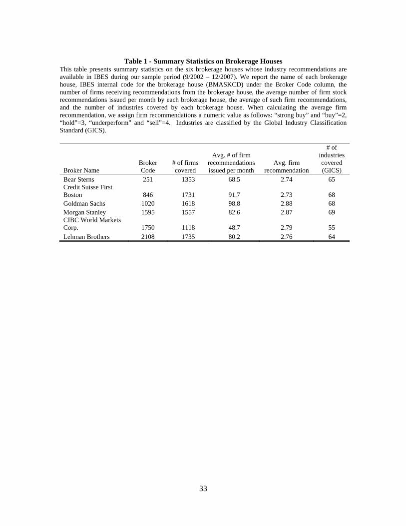
33

Table 1 - Summary Statistics on Brokerage Houses

This table presents summary statistics on the six brokerage houses whose industry recommendations are available in IBES during our sample period (9/2002 – 12/2007). We report the name of each brokerage house, IBES internal code for the brokerage house (BMASKCD) under the Broker Code column, the number of firms receiving recommendations from the brokerage house, the average number of firm stock recommendations issued per month by each brokerage house, the average of such firm recommendations, and the number of industries covered by each brokerage house. When calculating the average firm recommendation, we assign firm recommendations a numeric value as follows: “strong buy” and “buy”=2, “hold”=3, “underperform” and “sell”=4. Industries are classified by the Global Industry Classification Standard (GICS).

Broker Name Broker Code

# of firms covered

Avg. # of firm recommendations issued per month

Avg. firm recommendation

# of industries covered (GICS)

Bear Sterns 251 1353 68.5 2.74 65 Credit Suisse First Boston 846 1731 91.7 2.73 68 Goldman Sachs 1020 1618 98.8 2.88 68 Morgan Stanley 1595 1557 82.6 2.87 69 CIBC World Markets Corp. 1750 1118 48.7 2.79 55 Lehman Brothers 2108 1735 80.2 2.76 64

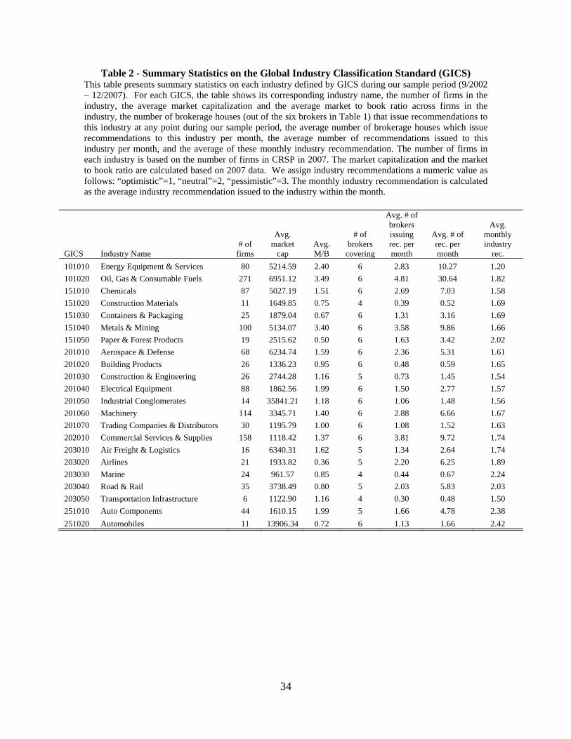
34

Table 2 - Summary Statistics on the Global Industry Classification Standard (GICS) This table presents summary statistics on each industry defined by GICS during our sample period (9/2002 – 12/2007). For each GICS, the table shows its corresponding industry name, the number of firms in the industry, the average market capitalization and the average market to book ratio across firms in the industry, the number of brokerage houses (out of the six brokers in Table 1) that issue recommendations to this industry at any point during our sample period, the average number of brokerage houses which issue recommendations to this industry per month, the average number of recommendations issued to this industry per month, and the average of these monthly industry recommendation. The number of firms in each industry is based on the number of firms in CRSP in 2007. The market capitalization and the market to book ratio are calculated based on 2007 data. We assign industry recommendations a numeric value as follows: “optimistic”=1, “neutral”=2, “pessimistic”=3. The monthly industry recommendation is calculated as the average industry recommendation issued to the industry within the month.

GICS Industry Name # of

firms

Avg. market

cap Avg. M/B

# of brokers

covering

Avg. # of brokers issuing rec. per month

Avg. # of rec. per month

Avg. monthly industry

rec.

101010 Energy Equipment & Services 80 5214.59 2.40 6 2.83 10.27 1.20

101020 Oil, Gas & Consumable Fuels 271 6951.12 3.49 6 4.81 30.64 1.82

151010 Chemicals 87 5027.19 1.51 6 2.69 7.03 1.58

151020 Construction Materials 11 1649.85 0.75 4 0.39 0.52 1.69

151030 Containers & Packaging 25 1879.04 0.67 6 1.31 3.16 1.69

151040 Metals & Mining 100 5134.07 3.40 6 3.58 9.86 1.66

151050 Paper & Forest Products 19 2515.62 0.50 6 1.63 3.42 2.02

201010 Aerospace & Defense 68 6234.74 1.59 6 2.36 5.31 1.61

201020 Building Products 26 1336.23 0.95 6 0.48 0.59 1.65

201030 Construction & Engineering 26 2744.28 1.16 5 0.73 1.45 1.54

201040 Electrical Equipment 88 1862.56 1.99 6 1.50 2.77 1.57

201050 Industrial Conglomerates 14 35841.21 1.18 6 1.06 1.48 1.56

201060 Machinery 114 3345.71 1.40 6 2.88 6.66 1.67

201070 Trading Companies & Distributors 30 1195.79 1.00 6 1.08 1.52 1.63

202010 Commercial Services & Supplies 158 1118.42 1.37 6 3.81 9.72 1.74

203010 Air Freight & Logistics 16 6340.31 1.62 5 1.34 2.64 1.74

203020 Airlines 21 1933.82 0.36 5 2.20 6.25 1.89

203030 Marine 24 961.57 0.85 4 0.44 0.67 2.24

203040 Road & Rail 35 3738.49 0.80 5 2.03 5.83 2.03

203050 Transportation Infrastructure 6 1122.90 1.16 4 0.30 0.48 1.50

251010 Auto Components 44 1610.15 1.99 5 1.66 4.78 2.38

251020 Automobiles 11 13906.34 0.72 6 1.13 1.66 2.42

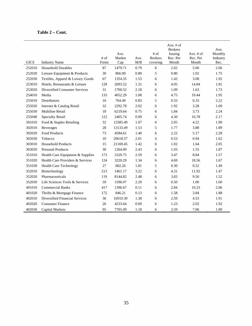
35

Table 2 – Cont.

GICS Industry Name # of

Firms

Ave. Market

Cap Ave. M/B

# of Brokers covering

Ave. # of Brokers Issuing

Rec. Per Month

Ave. # of Rec. Per Month

Ave. Monthly Industry

Rec.

252010 Household Durables 87 1479.71 0.79 6 2.02 5.00 2.06

252020 Leisure Equipment & Products 30 866.90 0.80 5 0.80 1.02 1.75

252030 Textiles, Apparel & Luxury Goods 67 1354.35 1.53 6 1.42 3.08 1.92

253010 Hotels, Restaurants & Leisure 128 2693.52 1.31 6 4.05 14.84 1.81

253020 Diversified Consumer Services 31 1700.52 2.18 6 1.09 1.63 1.73

254010 Media 133 4052.29 1.08 6 4.75 19.44 1.95

255010 Distributors 16 764.40 0.83 5 0.33 0.33 2.22

255020 Internet & Catalog Retail 32 2292.78 2.02 6 1.92 3.28 1.69

255030 Multiline Retail 18 6219.64 0.75 6 1.84 3.73 2.24

255040 Specialty Retail 122 2405.74 0.99 6 4.30 16.78 2.17

301010 Food & Staples Retailing 32 12585.49 1.07 6 2.05 4.22 1.90

302010 Beverages 28 13133.49 1.53 5 1.77 3.88 1.89

302020 Food Products 73 4584.61 1.40 6 2.22 5.17 2.28

302030 Tobacco 10 20618.57 2.01 4 0.53 0.94 1.62

303010 Household Products 15 21169.45 1.42 6 1.02 1.64 2.05

303020 Personal Products 30 1264.09 2.43 6 1.03 1.55 1.87

351010 Health Care Equipment & Supplies 173 2329.75 2.59 6 3.47 8.84 1.57

351020 Health Care Providers & Services 124 3220.29 1.34 6 4.69 18.56 1.67

351030 Health Care Technology 27 682.26 1.81 5 0.30 0.52 1.49

352010 Biotechnology 213 1461.17 3.22 6 4.31 11.92 1.47

352020 Pharmaceuticals 119 8144.82 2.48 6 3.83 9.56 1.52

352030 Life Sciences Tools & Services 59 1596.07 2.29 6 0.50 1.00 1.60

401010 Commercial Banks 417 1396.67 0.11 6 2.84 10.23 2.06

401020 Thrifts & Mortgage Finance 172 846.21 0.13 6 1.58 3.84 1.88

402010 Diversified Financial Services 36 16910.30 1.38 6 2.59 4.53 1.91

402020 Consumer Finance 26 4233.64 0.69 6 1.23 2.02 1.92

402030 Capital Markets 95 7705.09 1.18 6 2.59 7.06 1.89

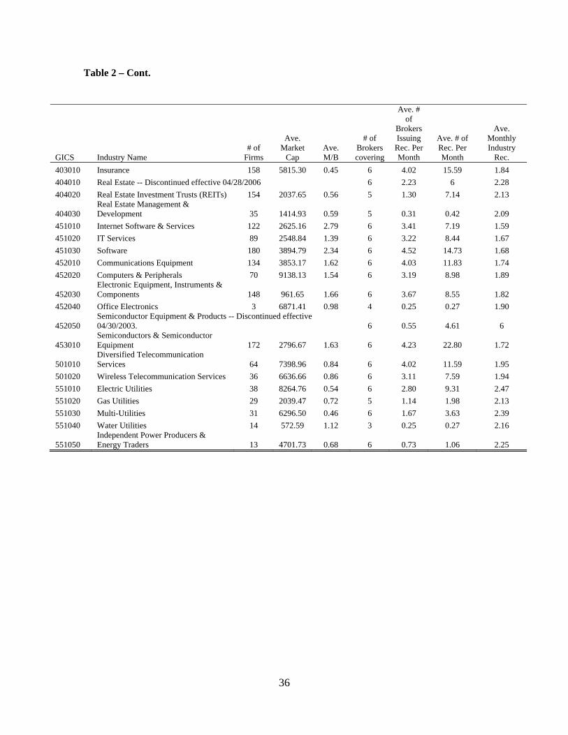
36

Table 2 – Cont.

GICS Industry Name # of

Firms

Ave. Market

Cap Ave. M/B

# of Brokers covering

Ave. # of

Brokers Issuing

Rec. Per Month

Ave. # of Rec. Per Month

Ave. Monthly Industry

Rec.

403010 Insurance 158 5815.30 0.45 6 4.02 15.59 1.84

404010 Real Estate -- Discontinued effective 04/28/2006 6 2.23 6 2.28

404020 Real Estate Investment Trusts (REITs) 154 2037.65 0.56 5 1.30 7.14 2.13

404030 Real Estate Management & Development 35 1414.93 0.59 5 0.31 0.42 2.09

451010 Internet Software & Services 122 2625.16 2.79 6 3.41 7.19 1.59

451020 IT Services 89 2548.84 1.39 6 3.22 8.44 1.67

451030 Software 180 3894.79 2.34 6 4.52 14.73 1.68

452010 Communications Equipment 134 3853.17 1.62 6 4.03 11.83 1.74

452020 Computers & Peripherals 70 9138.13 1.54 6 3.19 8.98 1.89

452030 Electronic Equipment, Instruments & Components 148 961.65 1.66 6 3.67 8.55 1.82

452040 Office Electronics 3 6871.41 0.98 4 0.25 0.27 1.90

452050 Semiconductor Equipment & Products -- Discontinued effective 04/30/2003. 6 0.55 4.61 6

453010 Semiconductors & Semiconductor Equipment 172 2796.67 1.63 6 4.23 22.80 1.72

501010 Diversified Telecommunication Services 64 7398.96 0.84 6 4.02 11.59 1.95

501020 Wireless Telecommunication Services 36 6636.66 0.86 6 3.11 7.59 1.94

551010 Electric Utilities 38 8264.76 0.54 6 2.80 9.31 2.47

551020 Gas Utilities 29 2039.47 0.72 5 1.14 1.98 2.13

551030 Multi-Utilities 31 6296.50 0.46 6 1.67 3.63 2.39

551040 Water Utilities 14 572.59 1.12 3 0.25 0.27 2.16

551050 Independent Power Producers & Energy Traders 13 4701.73 0.68 6 0.73 1.06 2.25

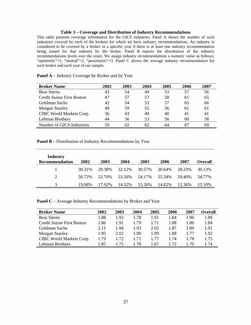
37

Table 3 – Coverage and Distribution of Industry Recommendations This table presents coverage information for the GICS industries. Panel A shows the number of such industries covered by each of the brokers for which we have industry recommendations. An industry is considered to be covered by a broker in a specific year if there is at least one industry recommendation being issued for that industry by the broker. Panel B reports the distribution of the industry recommendations levels over the years. We assign industry recommendations a numeric value as follows: “optimistic”=1, “neutral”=2, “pessimistic”=3. Panel C shows the average industry recommendation for each broker and each year of our sample. Panel A – Industry Coverage by Broker and by Year Broker Name 2002 2003 2004 2005 2006 2007Bear Sterns 43 54 49 53 57 56 Credit Suisse First Boston 47 57 57 58 61 65Goldman Sachs 42 54 53 57 65 66Morgan Stanley 49 59 55 56 61 61CIBC World Markets Corp. 36 43 40 40 41 41Lehman Brothers 44 56 53 56 60 58Number of GICS Industries 59 62 62 64 67 69

Panel B – Distribution of Industry Recommendations by Year

Industry Recommendation 2002 2003 2004 2005 2006 2007 Overall

1 30.21% 29.38% 32.12% 30.57% 30.64% 28.23% 30.13%

2 50.72% 52.70% 53.56% 54.17% 55.34% 59.40% 54.77%

3 19.08% 17.92% 14.32% 15.26% 14.02% 12.36% 15.10% Panel C – Average Industry Recommendations by Broker and Year Broker Name 2002 2003 2004 2005 2006 2007 OverallBear Sterns 1.88 1.93 1.78 1.91 1.84 1.96 1.89 Credit Suisse First Boston 1.86 1.91 1.79 1.71 1.88 1.86 1.84 Goldman Sachs 2.11 1.94 1.93 2.02 1.87 1.89 1.91 Morgan Stanley 1.95 2.02 1.90 1.99 1.88 1.77 1.92 CIBC World Markets Corp. 1.79 1.72 1.71 1.77 1.74 1.78 1.75 Lehman Brothers 1.85 1.75 1.78 1.67 1.72 1.70 1.74

38

Table 4 – Determinants of Industry Recommendations This table reports the results of estimating to logistic models of the probabilities of issuing an optimistic or pessimistic industry recommendations. The models are estimated for all industry recommendations issued during our sample period (9/2002-12/2007). The independent variables are as follows: Industry_Size is the natural logarithm of the aggregate market capitalization of the industry, MB is the industry weighted average of the market-to-book ratio, Profit is the industry weighted average of net income margin, R&D is the industry weighted average of the R&D divided by sales, Capex is the industry weighted average of the capital expenditures divided by sales. All weighted averages are by the firm market-capitalization at the beginning of the year in which a recommendation is issued. IND_RET is the return to an industry index in the previous quarters (up to three quarters back). MKT_RET is the market return in the previous quarters (up to three quarters back). TOTAL_IPOSEO is the total IPO/SEO proceeds in the industry during the year preceding the recommendation. AVG_IPOSEO is the average IPO/SEO proceeds in the industry during the year preceding the recommendation. IPOSEO_PCT is the percentage of IPO/SEO proceeds in an industry underwritten by the issuing broker during the year preceding the recommendation. In both specifications we control for broker fixed-effects. Robust standard errors (in parentheses) are calculated after clustering at the broker-industry level. ***, **, * denote statistical significance at the 1%, 5%, and 10% levels, respectively. Table appears in the next page.

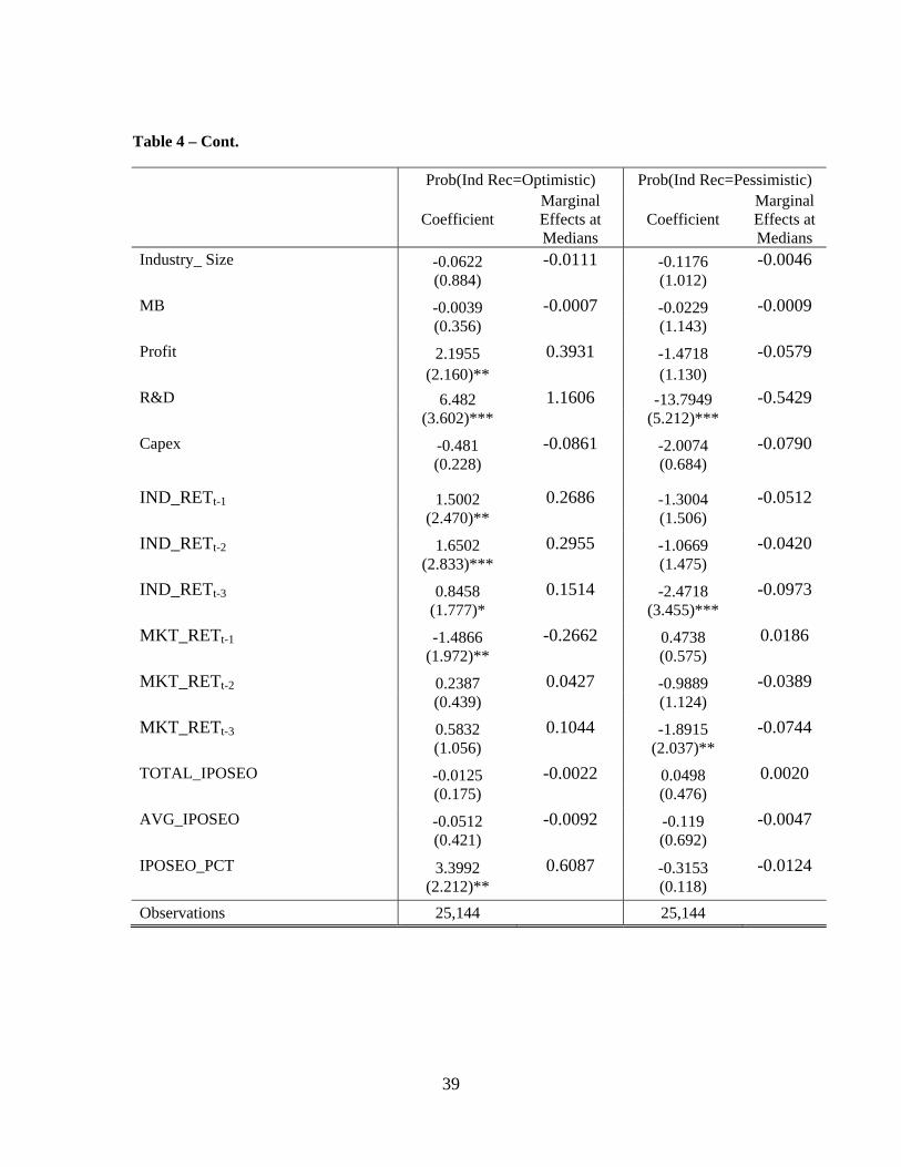
39

Table 4 – Cont.

Prob(Ind Rec=Optimistic) Prob(Ind Rec=Pessimistic)

Coefficient Marginal Effects at Medians

Coefficient Marginal Effects at Medians

Industry_ Size -0.0622 -0.0111 -0.1176 -0.0046 (0.884) (1.012) MB -0.0039 -0.0007 -0.0229 -0.0009 (0.356) (1.143) Profit 2.1955 0.3931 -1.4718 -0.0579 (2.160)** (1.130) R&D 6.482 1.1606 -13.7949 -0.5429 (3.602)*** (5.212)*** Capex -0.481 -0.0861 -2.0074 -0.0790

(0.228) (0.684)

IND_RETt-1 1.5002 0.2686 -1.3004 -0.0512 (2.470)** (1.506) IND_RETt-2 1.6502 0.2955 -1.0669 -0.0420 (2.833)*** (1.475) IND_RETt-3 0.8458 0.1514 -2.4718 -0.0973 (1.777)* (3.455)*** MKT_RETt-1 -1.4866 -0.2662 0.4738 0.0186 (1.972)** (0.575) MKT_RETt-2 0.2387 0.0427 -0.9889 -0.0389 (0.439) (1.124) MKT_RETt-3 0.5832 0.1044 -1.8915 -0.0744 (1.056) (2.037)** TOTAL_IPOSEO -0.0125 -0.0022 0.0498 0.0020 (0.175) (0.476) AVG_IPOSEO -0.0512 -0.0092 -0.119 -0.0047 (0.421) (0.692) IPOSEO_PCT 3.3992 0.6087 -0.3153 -0.0124 (2.212)** (0.118)

Observations 25,144 25,144

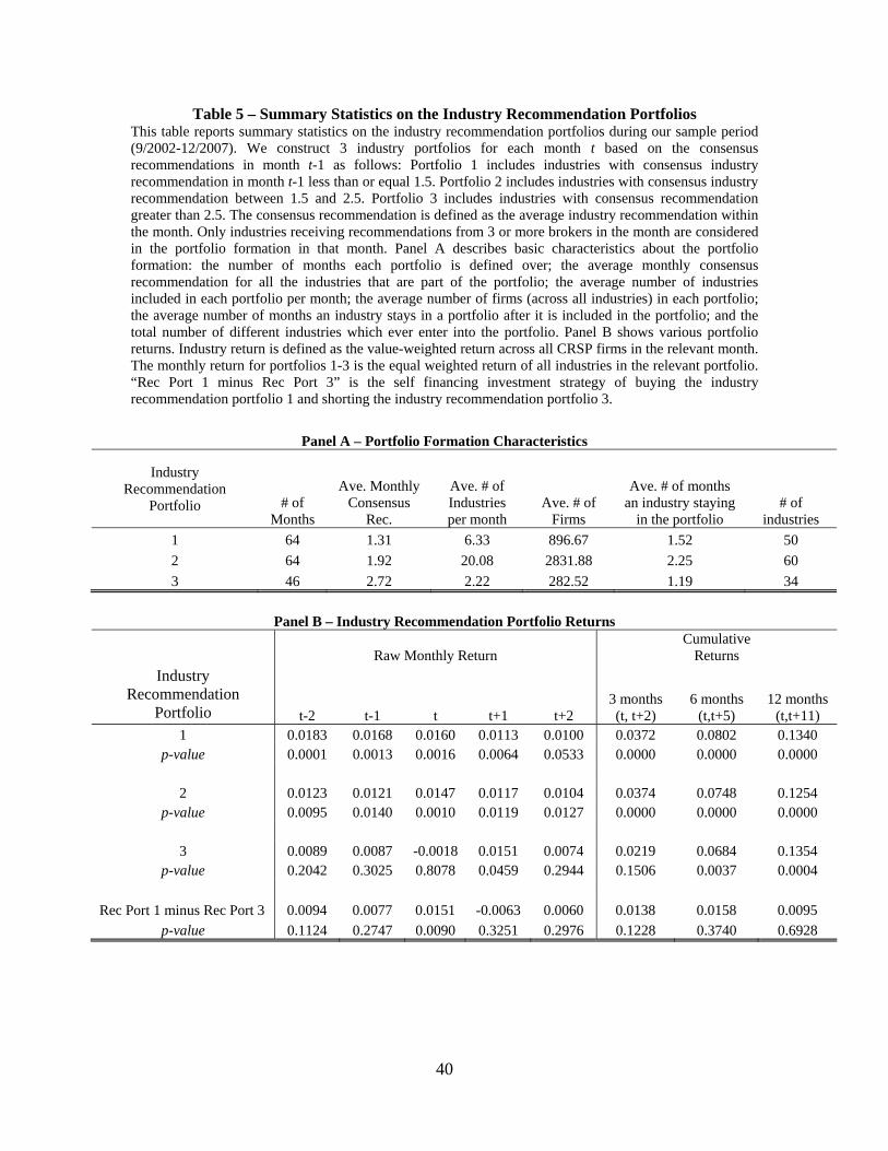
40

Table 5 – Summary Statistics on the Industry Recommendation Portfolios This table reports summary statistics on the industry recommendation portfolios during our sample period (9/2002-12/2007). We construct 3 industry portfolios for each month t based on the consensus recommendations in month t-1 as follows: Portfolio 1 includes industries with consensus industry recommendation in month t-1 less than or equal 1.5. Portfolio 2 includes industries with consensus industry recommendation between 1.5 and 2.5. Portfolio 3 includes industries with consensus recommendation greater than 2.5. The consensus recommendation is defined as the average industry recommendation within the month. Only industries receiving recommendations from 3 or more brokers in the month are considered in the portfolio formation in that month. Panel A describes basic characteristics about the portfolio formation: the number of months each portfolio is defined over; the average monthly consensus recommendation for all the industries that are part of the portfolio; the average number of industries included in each portfolio per month; the average number of firms (across all industries) in each portfolio; the average number of months an industry stays in a portfolio after it is included in the portfolio; and the total number of different industries which ever enter into the portfolio. Panel B shows various portfolio returns. Industry return is defined as the value-weighted return across all CRSP firms in the relevant month. The monthly return for portfolios 1-3 is the equal weighted return of all industries in the relevant portfolio. “Rec Port 1 minus Rec Port 3” is the self financing investment strategy of buying the industry recommendation portfolio 1 and shorting the industry recommendation portfolio 3.

Panel A – Portfolio Formation Characteristics

Industry Recommendation

Portfolio # of Months

Ave. Monthly Consensus

Rec.

Ave. # of Industries per month

Ave. # of Firms

Ave. # of months an industry staying

in the portfolio # of

industries

1 64 1.31 6.33 896.67 1.52 50

2 64 1.92 20.08 2831.88 2.25 60

3 46 2.72 2.22 282.52 1.19 34

Panel B – Industry Recommendation Portfolio Returns

Raw Monthly Return Cumulative

Returns

Industry Recommendation

Portfolio t-2 t-1 t t+1 t+2 3 months (t, t+2)

6 months (t,t+5)

12 months (t,t+11)

1 0.0183 0.0168 0.0160 0.0113 0.0100 0.0372 0.0802 0.1340 p-value 0.0001 0.0013 0.0016 0.0064 0.0533 0.0000 0.0000 0.0000

2 0.0123 0.0121 0.0147 0.0117 0.0104 0.0374 0.0748 0.1254

p-value 0.0095 0.0140 0.0010 0.0119 0.0127 0.0000 0.0000 0.0000

3 0.0089 0.0087 -0.0018 0.0151 0.0074 0.0219 0.0684 0.1354 p-value 0.2042 0.3025 0.8078 0.0459 0.2944 0.1506 0.0037 0.0004

Rec Port 1 minus Rec Port 3 0.0094 0.0077 0.0151 -0.0063 0.0060 0.0138 0.0158 0.0095 p-value 0.1124 0.2747 0.0090 0.3251 0.2976 0.1228 0.3740 0.6928

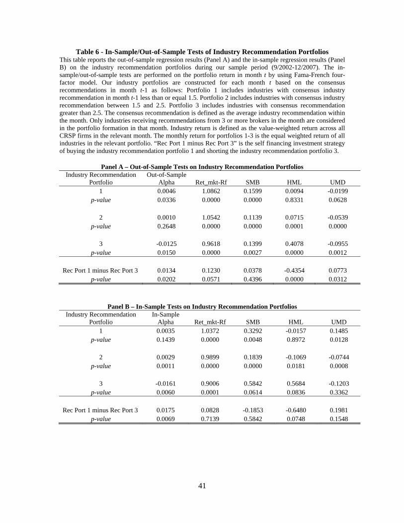
41

Table 6 - In-Sample/Out-of-Sample Tests of Industry Recommendation Portfolios This table reports the out-of-sample regression results (Panel A) and the in-sample regression results (Panel B) on the industry recommendation portfolios during our sample period (9/2002-12/2007). The in-sample/out-of-sample tests are performed on the portfolio return in month t by using Fama-French four-factor model. Our industry portfolios are constructed for each month t based on the consensus recommendations in month t-1 as follows: Portfolio 1 includes industries with consensus industry recommendation in month t-1 less than or equal 1.5. Portfolio 2 includes industries with consensus industry recommendation between 1.5 and 2.5. Portfolio 3 includes industries with consensus recommendation greater than 2.5. The consensus recommendation is defined as the average industry recommendation within the month. Only industries receiving recommendations from 3 or more brokers in the month are considered in the portfolio formation in that month. Industry return is defined as the value-weighted return across all CRSP firms in the relevant month. The monthly return for portfolios 1-3 is the equal weighted return of all industries in the relevant portfolio. “Rec Port 1 minus Rec Port 3” is the self financing investment strategy of buying the industry recommendation portfolio 1 and shorting the industry recommendation portfolio 3.

Panel A – Out-of-Sample Tests on Industry Recommendation Portfolios Industry Recommendation

Portfolio Out-of-Sample

Alpha Ret_mkt-Rf SMB HML UMD 1 0.0046 1.0862 0.1599 0.0094 -0.0199

p-value 0.0336 0.0000 0.0000 0.8331 0.0628

2 0.0010 1.0542 0.1139 0.0715 -0.0539 p-value 0.2648 0.0000 0.0000 0.0001 0.0000

3 -0.0125 0.9618 0.1399 0.4078 -0.0955

p-value 0.0150 0.0000 0.0027 0.0000 0.0012

Rec Port 1 minus Rec Port 3 0.0134 0.1230 0.0378 -0.4354 0.0773 p-value 0.0202 0.0571 0.4396 0.0000 0.0312

Panel B – In-Sample Tests on Industry Recommendation Portfolios Industry Recommendation

Portfolio In-Sample

Alpha Ret_mkt-Rf SMB HML UMD 1 0.0035 1.0372 0.3292 -0.0157 0.1485

p-value 0.1439 0.0000 0.0048 0.8972 0.0128

2 0.0029 0.9899 0.1839 -0.1069 -0.0744 p-value 0.0011 0.0000 0.0000 0.0181 0.0008

3 -0.0161 0.9006 0.5842 0.5684 -0.1203

p-value 0.0060 0.0001 0.0614 0.0836 0.3362

Rec Port 1 minus Rec Port 3 0.0175 0.0828 -0.1853 -0.6480 0.1981 p-value 0.0069 0.7139 0.5842 0.0748 0.1548

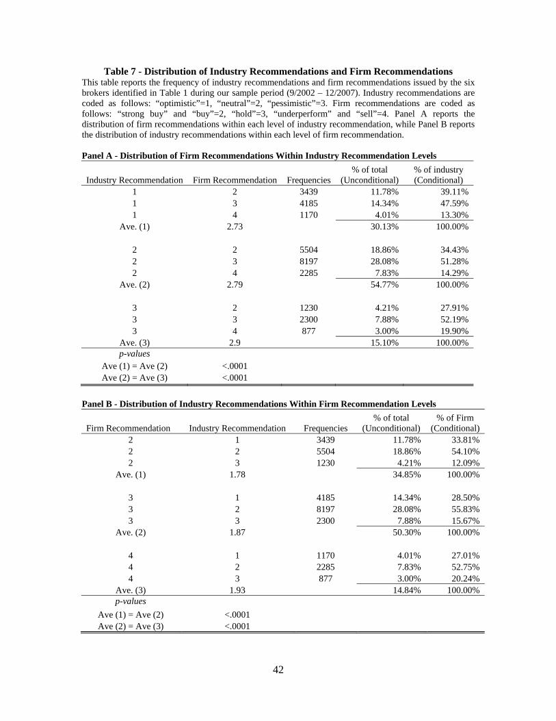
42

Table 7 - Distribution of Industry Recommendations and Firm Recommendations This table reports the frequency of industry recommendations and firm recommendations issued by the six brokers identified in Table 1 during our sample period (9/2002 – 12/2007). Industry recommendations are coded as follows: “optimistic”=1, “neutral”=2, “pessimistic”=3. Firm recommendations are coded as follows: “strong buy” and “buy”=2, “hold”=3, “underperform” and “sell”=4. Panel A reports the distribution of firm recommendations within each level of industry recommendation, while Panel B reports the distribution of industry recommendations within each level of firm recommendation. Panel A - Distribution of Firm Recommendations Within Industry Recommendation Levels

Industry Recommendation Firm Recommendation Frequencies% of total

(Unconditional) % of industry (Conditional)

1 2 3439 11.78% 39.11% 1 3 4185 14.34% 47.59% 1 4 1170 4.01% 13.30%

Ave. (1) 2.73 30.13% 100.00% 2 2 5504 18.86% 34.43% 2 3 8197 28.08% 51.28% 2 4 2285 7.83% 14.29%

Ave. (2) 2.79 54.77% 100.00% 3 2 1230 4.21% 27.91% 3 3 2300 7.88% 52.19% 3 4 877 3.00% 19.90%

Ave. (3) 2.9 15.10% 100.00% p-values

Ave (1) = Ave (2) <.0001 Ave (2) = Ave (3) <.0001

Panel B - Distribution of Industry Recommendations Within Firm Recommendation Levels

Firm Recommendation Industry Recommendation

Frequencies % of total

(Unconditional) % of Firm

(Conditional) 2 1 3439 11.78% 33.81% 2 2 5504 18.86% 54.10% 2 3 1230 4.21% 12.09%

Ave. (1) 1.78 34.85% 100.00%

3 1 4185 14.34% 28.50% 3 2 8197 28.08% 55.83% 3 3 2300 7.88% 15.67%

Ave. (2) 1.87 50.30% 100.00%

4 1 1170 4.01% 27.01% 4 2 2285 7.83% 52.75% 4 3 877 3.00% 20.24%

Ave. (3) 1.93 14.84% 100.00% p-values

Ave (1) = Ave (2) <.0001 Ave (2) = Ave (3) <.0001

43

Table 8 – Analysts’ disclosure about the meaning of firm recommendations This table reports information regarding the nature of firm recommendations, as it is disclosed by the brokerage houses. We include the 20 largest brokers in terms of the number of recommendations they issued between 2003 and 2007. In addition to the brokerage name and the percentage of recommendations, we indicate whether the recommendations are benchmarked to the industry. We also include an example of the original remark about the adopted benchmark by the brokerage house.

# Brokerage

House

% of recs. 2003-2007

Benchmark is Industry? Remarks about the benchmark

1 Argus

Research 1.5% No “We will generally rate a stock a buy if, in our view, the forecast risk-

adjusted return on the stock is greater than the forecast return on the market.”

2 Bear 2.5% Yes "Stock's expected performance vs analyst's industry coverage for the next 12

months."

3 RBC 1.4% Yes

“The rating assigned to a particular stock represents solely the analyst's view of how that stock will perform over the next 12 months relative to the

analyst's sector”

4 UBS 4.2% No

“The UBS rating system begins with the analyst determining the forecast stock return over the next 12 months. The forecast stock return relative to a predefined hurdle rate determines the Recommendation (Buy, Neutral, or Sell). This hurdle rate is set on either side of an unbiased estimate of the

market’s return over the next 12 months.”

5 Credit Suisse First Boston 3.4% Yes “Stock's expected total return vs. the industry for the next 12 months.”

6 Goldman

Sachs 3.7% Yes “Our ratings reflect expected stock price performance relative to each

analyst's coverage universe.”

7 JP Morgan 3.0% Yes

“Overweight: Over the next six to twelve months, we expect this stock will outperform the average total return of the stocks in the analyst’s (or the

analyst’s team’s) coverage universe.”

8 Jefferies and

Co. 1.5% No “Buy: describes stocks that we expect to provide a total return of 15% or

more within a 12-month period.”

9 Deutsche Bank 1.9% No “Buy: total return expected to appreciate 10% or more over a 12-month

period.”

10 Merrill Lynch 3.7% No “Based on stock's expected total return within a 12 month period.”

11 Morgan Stanley 2.7% Yes

“Stock's total return vs. analyst's coverage on a risk-adjusted basis, for the next 12-18 months.”

12 CIBC 1.7% Yes “Stock's expected performance vs the sector for the next 12-18 months.”

13 US Bancorp Piper Jaffray 2.0% No Performance “relative to the market index over the next 12 months.”

14 Raymond

James 1.8% No Performance “relative to the market index over the next 12 months.”

15 Lehman Brothers 2.8% Yes “Stock's performance vs. the industry for a 12 month investment horizon”

16 Smith Barney 3.4% Yes “Stock's performance vs. the analyst's industry coverage for the coming 12-18

months.”

17 Stifel Nicolaus 1.4% No “Performance “relative to S&P 500 over the next 12 months.”

18 Wachovia 1.9% No Performance “relative to the market over the next 12 months.”

19 Friedman

Billing 1.5% Yes Performance “relative to similar companies within its industry over the next

12-18 months.”

20 Banc of America 1.8% No

“The rating system is based on a stock's forward -12-month expected total return (price appreciation plus dividend yield).”

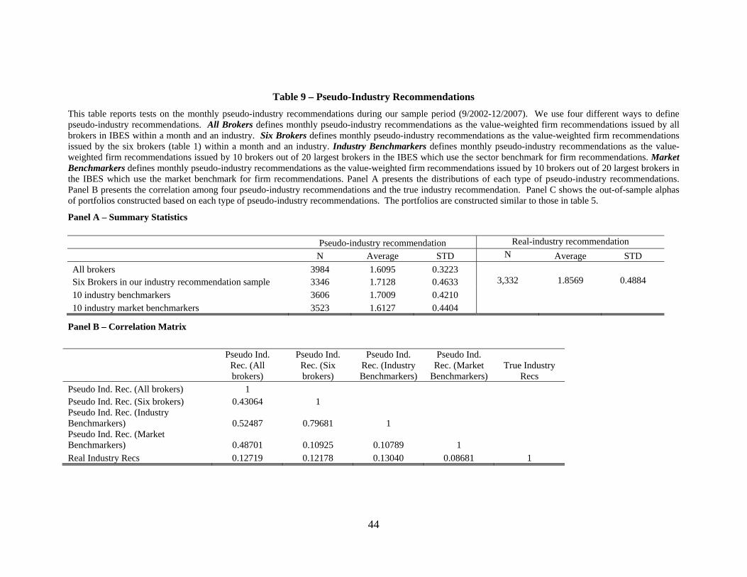
44

Table 9 – Pseudo-Industry Recommendations

This table reports tests on the monthly pseudo-industry recommendations during our sample period (9/2002-12/2007). We use four different ways to define pseudo-industry recommendations. All Brokers defines monthly pseudo-industry recommendations as the value-weighted firm recommendations issued by all brokers in IBES within a month and an industry. Six Brokers defines monthly pseudo-industry recommendations as the value-weighted firm recommendations issued by the six brokers (table 1) within a month and an industry. Industry Benchmarkers defines monthly pseudo-industry recommendations as the value-weighted firm recommendations issued by 10 brokers out of 20 largest brokers in the IBES which use the sector benchmark for firm recommendations. Market Benchmarkers defines monthly pseudo-industry recommendations as the value-weighted firm recommendations issued by 10 brokers out of 20 largest brokers in the IBES which use the market benchmark for firm recommendations. Panel A presents the distributions of each type of pseudo-industry recommendations. Panel B presents the correlation among four pseudo-industry recommendations and the true industry recommendation. Panel C shows the out-of-sample alphas of portfolios constructed based on each type of pseudo-industry recommendations. The portfolios are constructed similar to those in table 5.

Panel A – Summary Statistics Pseudo-industry recommendation Real-industry recommendation

N Average STD N Average STD

All brokers 3984 1.6095 0.3223

Six Brokers in our industry recommendation sample 3346 1.7128 0.4633 3,332 1.8569 0.4884

10 industry benchmarkers 3606 1.7009 0.4210

10 industry market benchmarkers 3523 1.6127 0.4404

Panel B – Correlation Matrix

Pseudo Ind. Rec. (All brokers)

Pseudo Ind. Rec. (Six brokers)

Pseudo Ind. Rec. (Industry Benchmarkers)

Pseudo Ind. Rec. (Market

Benchmarkers) True Industry

Recs Pseudo Ind. Rec. (All brokers) 1 Pseudo Ind. Rec. (Six brokers) 0.43064 1 Pseudo Ind. Rec. (Industry Benchmarkers) 0.52487 0.79681

1

Pseudo Ind. Rec. (Market Benchmarkers) 0.48701 0.10925 0.10789

1

Real Industry Recs 0.12719 0.12178 0.13040 0.08681 1

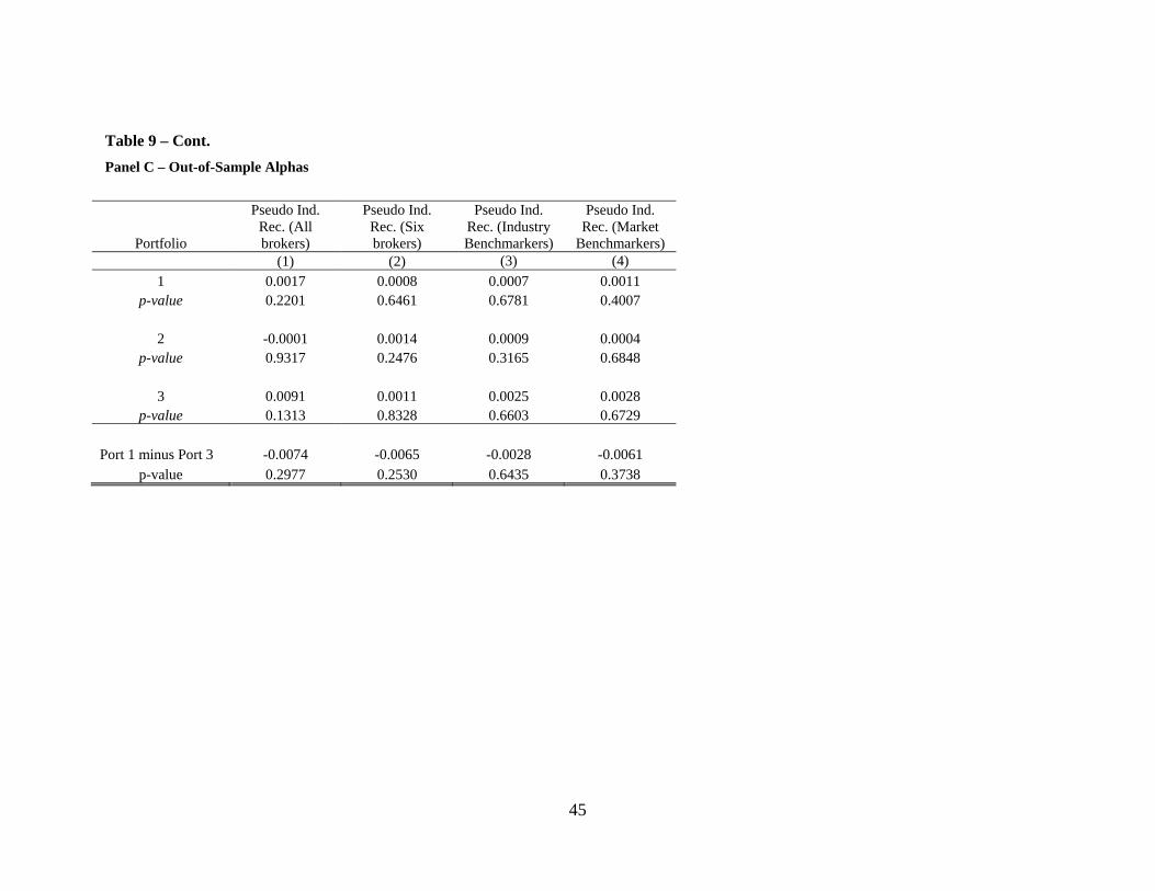
45

Table 9 – Cont.

Panel C – Out-of-Sample Alphas

Portfolio

Pseudo Ind. Rec. (All brokers)

Pseudo Ind. Rec. (Six brokers)

Pseudo Ind. Rec. (Industry Benchmarkers)

Pseudo Ind. Rec. (Market

Benchmarkers) (1) (2) (3) (4)

1 0.0017 0.0008 0.0007 0.0011 p-value 0.2201 0.6461 0.6781 0.4007

2 -0.0001 0.0014 0.0009 0.0004

p-value 0.9317 0.2476 0.3165 0.6848 3 0.0091 0.0011 0.0025 0.0028

p-value 0.1313 0.8328 0.6603 0.6729

Port 1 minus Port 3 -0.0074 -0.0065 -0.0028 -0.0061 p-value 0.2977 0.2530 0.6435 0.3738

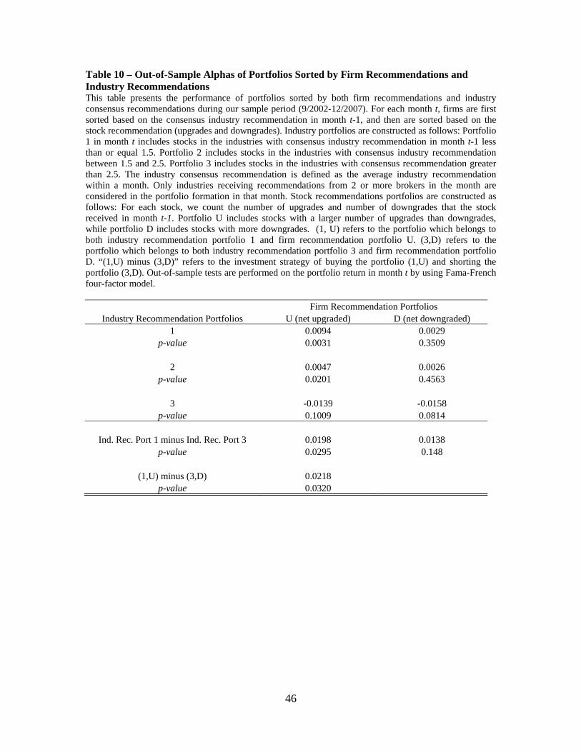
46

Table 10 – Out-of-Sample Alphas of Portfolios Sorted by Firm Recommendations and Industry Recommendations This table presents the performance of portfolios sorted by both firm recommendations and industry consensus recommendations during our sample period (9/2002-12/2007). For each month t, firms are first sorted based on the consensus industry recommendation in month t-1, and then are sorted based on the stock recommendation (upgrades and downgrades). Industry portfolios are constructed as follows: Portfolio 1 in month t includes stocks in the industries with consensus industry recommendation in month t-1 less than or equal 1.5. Portfolio 2 includes stocks in the industries with consensus industry recommendation between 1.5 and 2.5. Portfolio 3 includes stocks in the industries with consensus recommendation greater than 2.5. The industry consensus recommendation is defined as the average industry recommendation within a month. Only industries receiving recommendations from 2 or more brokers in the month are considered in the portfolio formation in that month. Stock recommendations portfolios are constructed as follows: For each stock, we count the number of upgrades and number of downgrades that the stock received in month t-1. Portfolio U includes stocks with a larger number of upgrades than downgrades, while portfolio D includes stocks with more downgrades. (1, U) refers to the portfolio which belongs to both industry recommendation portfolio 1 and firm recommendation portfolio U. (3,D) refers to the portfolio which belongs to both industry recommendation portfolio 3 and firm recommendation portfolio D. “(1,U) minus (3,D)” refers to the investment strategy of buying the portfolio (1,U) and shorting the portfolio (3,D). Out-of-sample tests are performed on the portfolio return in month t by using Fama-French four-factor model. Firm Recommendation Portfolios

Industry Recommendation Portfolios U (net upgraded) D (net downgraded) 1 0.0094 0.0029

p-value 0.0031 0.3509 2 0.0047 0.0026

p-value 0.0201 0.4563 3 -0.0139 -0.0158

p-value 0.1009 0.0814

Ind. Rec. Port 1 minus Ind. Rec. Port 3 0.0198 0.0138 p-value 0.0295 0.148

(1,U) minus (3,D) 0.0218

p-value 0.0320