Embed Size (px)
Citation preview
NBER WORKING PAPER SERIES
REAL EXCHANGE RATE FLUCTUATIONS AND THE DYNAMICS OF RETAIL TRADEINDUSTRIES ON THE U.S.-CANADA BORDER
Jeffrey R. CampbellBeverly Lapham
Working Paper 8558http://www.nber.org/papers/w8558
NATIONAL BUREAU OF ECONOMIC RESEARCH1050 Massachusetts Avenue
Cambridge, MA 02138October 2001
We thank Martin Boileau, Lars Hansen, Allen Head, Chad Syverson, and Oved Yosha for helpful commentson previous versions of this paper. The National Science Foundation supported Campbell's research throughgrant SBR-9730442, “Business Cycles and Industry Dynamics." The Social Science and HumanitiesResearch Council of Canada supported Lapham's research. Emin Dinlersoz provided expert researchassistance at an early stage of this project. The latest versions of this paper and its technical appendix areavailable on the World Wide Web at http://home.uchicago.edu/~jcampbe. Please direct correspondence toCampbell at Department of Economics, University of Chicago, 1126 East 59th Street, Chicago, Illinois60637. The views expressed herein are those of the authors and not necessarily those of the National Bureauof Economic Research.
© 2001 by Jeffrey R. Campbell and Beverly Lapham. All rights reserved. Short sections of text, not toexceed two paragraphs, may be quoted without explicit permission provided that full credit, including ©notice, is given to the source.
Real Exchange Rate Fluctuations and the Dynamics of Retail Trade Industrieson the U.S.-Canada BorderJeffrey R. Campbell and Beverly LaphamNBER Working Paper No. 8558October 2001JEL No. F4, E3, L8
ABSTRACT
Consumers living near the U.S.-Canada border can shift their expenditures between the two
countries, so real exchange rate fluctuations can act as demand shocks to border areas' retail trade
industries. Using annual county-level data, we estimate the effects of real exchange rates on the number
of establishments and their average payroll in border counties for four retail industries. In three of the four
industries we consider, the number of operating establishments responds either contemporaneously or
with a lag of one year to real exchange rate movements. For these industries, the response of retailers'
average size is less pronounced. The rapid response of net entry is inconsistent with any model of
persistent deviations from purchasing power parity that depends on retailers' costs of changing nominal
prices.
Jeffrey R. Campbell Beverly LaphamDepartment of Economics Department of EconomicsUniversity of Chicago Queen's University1126 East 59th Street Dunning HallChicago, IL 60637 Kingston, ON K7L 3N6and NBER [email protected] [email protected]

This paper estimates the effects of real exchange rate fluctuations on the number of
stores and their average payroll in retail trade industries located near the U.S.-Canada
border. Our empirical results address two basic questions concerning retailers’ short-run
and long-run responses to shocks: How important is retailers’ price stickiness for propagating
nominal shocks? How quickly does net entry respond to demand shocks? The answers to
these questions are related because it should take less time for an incumbent retailer to
change nominal prices than it does for a potential entrant to open a store. Macroeconomic
models featuring sticky nominal prices, such as Chari, Kehoe, and McGrattan’s (2000a) and
Christiano, Eichenbaum, and Evans’ (2001), embody this assumption by fixing the number
of producers over the relevant horizon. In these models, an industry that expands because
nominal disturbances erode the real value of fixed nominal prices displays increasing average
producer size and no increase in the number of producers. However, we find the opposite to
be true for two of the industries we examine that are known to display infrequent store-level
nominal price adjustments, Food Stores and Eating Places. For those industries, fluctuations
in the real exchange rate induce a change in the number of stores either contemporaneously
or with a lag of one year. Since the typical half-life of a deviation of the real exchange
rate from purchasing power parity is between three and four years, our results imply that
retail-level price stickiness cannot be primarily responsible for these observed international
price differences.
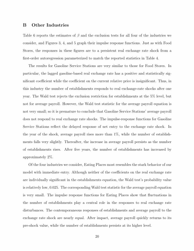
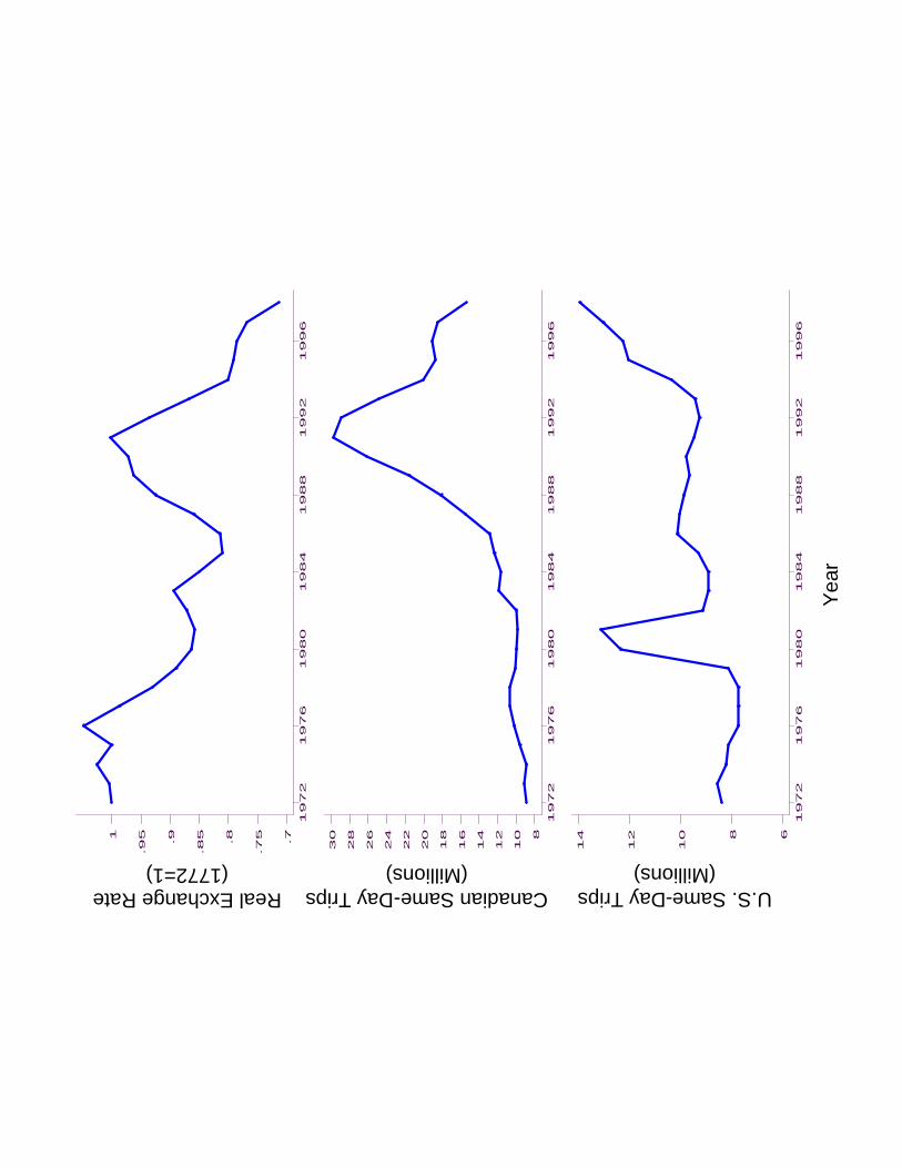
For retailers in border communities, real exchange rate fluctuations represent changes in
the price of a substitute good. Thus, they have effects similar to an ordinary demand shock.
Figure 1 illustrates these effects. Its top panel depicts the Canada-U.S. real exchange rate
between 1972 and 1998 (normalized to equal 1 in 1972), and its bottom two panels each
plot a measure of cross-border shoppers, the number of one-day trips by Canadians and
Americans to the other country. The strong Canadian dollar in the late 1980’s and early
1990’s induced a surge in the number of Canadian trips to the U.S. This reversed itself in the
middle of the 1990’s when the Canadian dollar depreciated and American trips to Canada
1

dramatically increased. The spike in American trips in 1980-1981 came at a time when the
Canadian National Energy Policy greatly reduced gasoline’s price in Canada relative to its
U.S. price. In response, American consumers’ living near the border shifted their gasoline
expenditures towards Canadian retailers.
We consider four industries for which travel costs relative to the value of a typical purchase
make ongoing international arbitrage impractical for consumers living very far away from the
U.S.-Canada border: Food Stores, Gasoline Service Stations, Eating Places, and Drinking
Places. For each of these industries, we estimate a panel-data vector autoregression using
annual county-level data on the number of retail establishments and their average annual
payroll from the ten contiguous states that border Canada. As explanatory variables, we
include current and lagged real exchange rates interacted with a measure of each county’s
sensitivity to real exchange rate fluctuations, derived from the model we consider in Section
I. Since the real exchange rate is an endogenous variable, determined by structural shocks
that can have direct effects on consumers’ purchasing decisions and retailers’ costs, we use
observations from counties off of the U.S.-Canada border to estimate coefficients on time
dummies that control for these direct effects. In this way, we use variation in counties’
proximity to the border to identify the expenditure-shifting effects of real exchange rates on
border counties’ retail trade industries. In all of the industries we study, we find that these
effects are significant.
The rest of this paper is organized as follows. In the next section, we present a model
of retail industry dynamics with cross-border shopping. Section II describes the model’s
empirical specification, the data, and the GMM estimation procedure we use. Section III
presents the estimation results, and Section IV discusses the relationship of our work with the
relevant literature from international macroeconomics and industrial organization. Section
V contains concluding remarks regarding our results’ implications for future research.
2

I A Cross-Border Shopping Model
To structure our empirical analysis, we develop a model of retail industry dynamics with
cross-border shopping. If neither retailers’ prices nor their entry decisions can respond to
the shocks driving real exchange rate fluctuations, then these shocks’ expenditure-shifting
effects can only change average store size and not the number of stores. The empirical
predictions of such a sticky-price model are already clear, so we incorporate into our model
the opposite assumptions of flexible retail price setting and free entry. We also describe below
the implications of combining these two models by assuming that some retailers’ nominal
prices are sticky while the prices and entry decisions of others can respond to all relevant
disturbances.
We use a partial equilibrium model of two counties: U located in the United States and
C located directly across the border in Canada. Each county has a retail-trade sector that
produces differentiated goods in a monopolistically-competitive market with free entry. Re-
tailers in both counties face no price rigidities and use identical constant-percentage markup
pricing rules, so deviations from PPP entirely reflect differences in retailers’ marginal costs.
Our model is a partial equilibrium model because we assume that the marginal costs of
retailers in U and C are determined in their respective national economies. Retailers’ cost
differences could arise from differences in retail technology, regulations which prevent ar-
bitrage in wholesale goods, nominal rigidities in manufacturers’ and wholesalers’ prices, or
some combination of these sources. Because consumers in border counties can choose where
to shop, deviations from PPP induce a shift of expenditures towards the less expensive
county. We analyze the response of both counties’ retail-trade industries to movements in
relative costs, focusing on the behavior of variables we observe in our data, the number of
establishments and their average payroll in the U.S. county.
3
A Consumers
There are Sj consumers in county j and a fraction, λ, of those consumers are travellers who
purchase from both domestic and foreign retailers. The remaining consumers in a county
can only purchase from domestic retailers and are referred to as non-travellers. Consumers
have the following preferences:
U = d1−γ(∫ NU
0xνiUdi+
∫ NC
0xνiCdi
) γν
,
where d is consumption of a homogeneous numeraire good and xij is consumption of dif-
ferentiated good i sold in county j ∈ {U,C}, and both γ and ν are strictly between zero
and one. For non-travellers, consumption of goods sold by foreign retailers equals zero. The
number of distinct goods offered for sale in county j is Nj and is determined in equilibrium.
All consumers are endowed with ω units of the numeraire good which they use to finance
consumption expenditures.
B Technology
Each retailer incurs a fixed cost of φ units of the numeraire good in each period. She also
uses labor and materials to produce her single distinct good using a technology with constant
marginal cost cj, j = U,C. The fractions of variable and fixed costs paid to labor are α and
δ, so the payroll of a retailer located in county j with output equal to x is
Wj = αcjx+ δφ.(1)
C Free-Entry Equilibrium
The retail production technology is available to large pools of potential entrants in both
countries. The marginal costs, cU and cC , are random variables that are exogenous from the
perspective of a single county’s retail sector. After observing cU and cC , potential entrants
simultaneously decide whether or not to irreversibly incur the fixed cost and produce. In
4

equilibrium those that enter choose their prices to maximize profits, and further entry is
not profitable in either location. For simplicity, we suppose retailers must incur the fixed
cost every period, so a border county’s retail-trade sector is characterized by the infinite
repetition of this free-entry game.1
The isoelasticity of consumers’ Marshallian demand curves implies that producers’ profit
maximizing prices will follow the familiar constant-percentage markup over marginal cost
rule:
pj =cjν,(2)
where pj is the price chosen by all retailers in county j. Combining this with the zero profit
condition and (1) yields each retailer’s equilibrium output, xj, and one of our observable
variables, average payroll.
xj =φν
cj (1− ν)(3)
Wj =αφν
1− ν+ δφ.(4)
Retailers’ average sizes in both counties (measured with either sales, pj × xj or payroll, Wj)
are constant, so all of the industry’s response to fluctuations in cU and cC must occur through
changes in the number of retailers on both sides of the border.
To determine NU and NC , we equate the output per retailer that is consistent with free-
entry from (3) with the output demanded by consumers at the prices given by (2). Doing
so yields
(1− λ)SUNU
+λ (SU + SC)
NU +NCrν/(ν−1) =φ
γω (1− ν)(5)
(1− λ)SCNC
+λ (SU + SC)
NUrν/(1−ν) +NC
=φ
γω (1− ν),(6)
where r ≡ (pC/pU), which we henceforth refer to as the industry real exchange rate.1With minor modifications, our analysis carries through if we instead assume that φ is a sunk cost of
entry and that incumbent establishments each face a constant probability of exogenous destruction.
5
If there were no cross-border shopping, then λ = 0 and finding the values of NU and NC
that satisfy (5) and (6) is straightforward. If r = 1 and λ > 0, then these equations have
the same solution as they do when λ = 0:
N̄j = Sjγω (1− ν)
φ, j ∈ {U,C}.(7)
That is, if the marginal costs in the two counties equal each other, the retail trade sector in
a border county should be no different from its counterpart in an interior county.
To determine the responses of NU and NC to changes in r, take a log-linear approximation
of (5) and (6) around the point r = 1, N̄U , N̄C . Solving the resulting equations yields
ln(NU/N̄U
)=[
νλ
(1− ν)(1− λ)
] [SC
SU + SC
]ln(r)(8)
ln(NC/N̄C
)=[
−νλ(1− ν)(1− λ)
] [SU
SU + SC
]ln(r)(9)
When a decrease in cU causes r to increase, the number of producers operating in county U
rises. Simultaneously, the number of producers in county C falls.
Because SU and SC vary across U.S. border counties, so will the second term in brackets
in (8). We refer to this term as the (U.S.) county’s sensitivity measure. As intuition suggests,
it is increasing in the population of Canadian consumers and decreasing in the population
of U.S. consumers. The sensitivity measure is an important component of our estimation.2
D Retail Industry Dynamics with Sticky Prices
Thus far, we have presumed that a stable industry structure is a prerequisite for price
stickiness of a meaningful duration. Nevertheless, both massive ongoing restructuring of
retail trade industries and infrequent nominal retail price changes have been independently2If we suppose that retailers’ entry decisions must be made before observing r, WU and WC will also
fluctuate when ln r differs from its expectation at the time of entry, and NU and NC will depend on past
values of ln r. The elasticities of WU and NU with respect to r and its past values are both proportional to
the sensitivity measure in (8), so the empirical approach we derive in Section II remains valid.
6
documented.3 For this reason, it may seem desirable to incorporate ongoing restructuring
into a model with sticky prices. In this vein, we have extended our model to include U.S.
and Canadian currencies and retailers in both counties that are “sticky.” This paper’s
technical appendix describes this extension in detail. Sticky retailers’ entry and nominal
pricing decisions must be made before any shock’s realization, while the “flexible” retailers
we have focused on above continue to have complete information for both of these choices.
In this environment, a nominal shock that lowers the real prices of sticky retailers in C but
does not change the relative real marginal costs between C and U induces a reduction in
the number of flexible retailers in C. The reduction in entry exactly offsets the effects of
sticky retailers’ price inflexibility, so that the correctly constructed aggregate price index
for C (which accounts for the change in variety) changes one for one with the nominal
disturbance. The real exchange rate is unchanged, so the Canadian nominal disturbance
has no expenditure shifting effects and no effects on the retail industry in U . This result
demonstrates that price stickiness and nominal shocks can generate expenditure shifting
between U and C only if it takes longer to implement an entry decision than it does to
change a nominal price.4
II Data and Estimation
The empirical model that we use for estimation is an extension of the model considered above
that accounts for county-specific and economy-wide disturbances to cost and demand as well
as unobserved heterogeneity across counties. The estimating equation uses the sensitivity
measure from (8), but it does not restrict real exchange rates to impact only the number of3See Foster, Haltiwanger, and Krizan (2001) for measurement of entry and exit in U.S. retail industries,
Lach and Tsiddon (1996) for evidence of infrequent price adjustment in Israeli food stores, and MacDonald
and Aaronson (2000) for similar evidence in U.S. Eating Places.4Including sticky retailers hardly alters the model’s predictions regarding changes in the relative real
marginal costs of retailers in U and C. In particular, the sensitivity measure in (8) remains appropriate.
7

retailers. Instead, it allows both the number of retailers and their average payroll to respond
to real exchange rates. This section explains the empirical model, describes the data we use,
and summarizes our GMM estimation procedure. We begin with the empirical model.
A The Empirical Model
We estimate our model separately for the four industries we consider. For each year and each
county in our sample we observe the number of establishments operating in the industry and
the U.S. dollar value of industry payroll. We also observe each county’s population in 1990.
For the industry of interest in county i, we define the vector
yit =[
lnNit lnWit
]′,
where Nit is the number of stores operating at any time during the year divided by the 1990
population of county i (establishments), and Wit is the dollar value of industry payroll for
the year divided by the number of establishments (average payroll). Our data set provides
annual observations of yit.
The estimating equation we use is
yit = αi + µt + Λyit−1 + β′ (si × et) + εit(10)
where αi is a random county-specific intercept, µt is a time-specific effect common to all
counties, Λ and β are (2× 2) matrices of unknown coefficients,
et =[
ln rt ln rt−1
]′,(11)
si =SiC
SiU + SiC,(12)
and εit is a disturbance term.5 In (12), SiU is the population of U.S. county i and SiC is a5The fixed effects in (10) allow us to use unscaled observations on the number of establishments rather
than the per capita measure we use. We chose the latter specification, however, because the GMM estimation
procedure described below treats αi as a component of the model’s error rather than as a parameter to be
estimated. Scaling establishments by population as the model suggests reduces the overall error variance.
8
measure of population in its Canadian counterpart. If county i does not share a border with
Canada, then we set SiC = 0.
Consider first the implications of (10) for counties that do not border Canada, which we
henceforth refer to as interior counties. In this case si = 0, and (10) implies that yit follows
a first-order vector autoregression (VAR) with intercept αi and disturbance term µt + εit.
We assume that the roots of |I − ΛL| lie outside of the unit circle and that if the county is
interior, then
E [εit] = 0,(13)
E [εitεiτ ] = 0 if t 6= τ,(14)
That is, for an interior county εit is the fundamental error (in the sense of the Wold decom-
position theorem) for yit − (I − ΛL)−1 µt. We furthermore assume that for interior counties
E [αi] = 0.(15)
Given the presence of µt in (10), this is only a normalization.
This specification for interior counties’ fluctuations can be derived from our model if we
suppose that each consumer’s income (ω) and each retailer’s fixed cost (φ) are subject to
county-specific disturbances that themselves follow a first-order VAR in logarithms. Under
this interpretation, the intercept term αi reflects these variables’ county-specific means. The
disturbance term’s common component, µt, embodies aggregate disturbances that effect all
counties uniformly. The economy-wide effects of any structural aggregate shock that causes
the real exchange rate to fluctuate will be incorporated into µt. There are no constraints on
µt, and we treat it as a parameter to be estimated.
To characterize the fluctuations in yit for border counties, we assume that their responses
to the aggregate disturbances in µt are identical to the responses of interior counties and that
the same autoregressive equation describes their dynamics in the absence of real exchange
rate fluctuations. For border counties the current and lagged real exchange rates interacted
9
with si are added to (10) as explanatory variables.6 We include the lagged real exchange rate
to allow the effects of a completely transitory disturbance to ln rt to be equally short-lived,
as they are in the (essentially static) model.
The real exchange rate between each U.S. border county and its Canadian counterpart
potentially varies across counties. Let rit denote the relative retail price between county i
and its Canadian counterpart. The location-specific price data needed to construct rit are
not available to us, so instead (10) uses its national-level analogue, rt. We further discuss
our measure of rt in Section C below. To replace rit with rt in the model, we suppose that
the linear projection of rit on rt has a slope coefficient of one for each border county. That
is
ln rit = ai + ln rt + ζit,(16)
where {ζit} is a mean-zero covariance-stationary stochastic process that is independent across
counties.7
The difference between rit and rt implies that the interpretations we have placed on εit
and αi for interior counties are inappropriate. Instead, εit now equals the the model’s true
error plus a measurement error term involving ζit and ζit−1, and αi equals the true intercept
plus a term involving ai. The presence of measurement error implies that (13) also applies to
εit for a border county, but (14) and (15) do not. The moment conditions we use to identify
the model’s parameters account for these differences between interior and border counties’
observations.
We now turn to the discussion of our observations of yit, rt, and si.6Note that we do not include the relative per capita consumption expenditures of U.S. and Canadian
consumers in (10). Although we assumed in Section I that consumers in counties U and C had the same
real consumption expenditures, this was only a simplification. Variation in relative per capita consumption
between U and C has no equilibrium impact on the retail industry in U , so its omission from (10) is not a
misspecification.7Equation (10) is also correct if instead the slope coefficient in (16) equals b 6= 1, but the interpretation
of β must be suitably altered to reflect the change in scale.
10
B Observations of Retail Trade Industries
Our observations of retail trade industries come from the United States Census’ annual
publication, County Business Patterns (CBP). We construct our data set from twenty years
of this publication from 1977 through 1996. We focus on counties in the ten contiguous
states that border Canada because we wish the sample’s interior counties to be as otherwise
similar as possible to the border counties. For each retail trade industry, the CBP reports
each county’s annual payroll and the number of establishments with employees, among other
variables. Because this data is based on administrative payroll tax records, its quality is very
high. Our empirical work uses the establishment count divided by the county’s population
in 1990 for Nit and uses annual payroll divided by the number of establishments for Wit.
Our discussion above has presumed that only those counties that share a border with
Canada are exposed to cross-border shopping. For some retail trade industries, this is clearly
not the case. For example, Ford (1992) surveyed Canadian consumers in Toronto, Hamilton,
and the Niagara-St. Catherines region regarding their shopping destinations in the U.S.
Many consumers reported shopping outside of the New York border counties of Erie and
Niagara, particularly if the shopping trips were for durable goods such as furniture and
electronics. Conversely, U.S. consumers from counties without a Canadian border can shop
in Canada if they are willing to travel. However, Ford’s (1992) survey data indicates that
purchasers of food and gasoline, the two most frequently purchased items by cross-border
shoppers, tended to shop very near the border. For this reason, we restrict our analysis
to retail trade industries that Ford’s (1992) data and our own experience as cross-border
shoppers indicate consumers are unwilling to travel far to purchase. The industries we
consider are Food Stores (SIC 54), Gasoline Service Stations (SIC 554), Eating Places (SIC
5812), and Drinking Places (SIC 5813).
Our data set is incomplete because the Census withholds the payroll information for any
county-industry observation where that datum may disclose information about any individ-
ual producer. The Census does not reveal how it determines which observations must be
11
withheld, but these disclosure cases tend to occur in counties with small populations and
few establishments. To produce a balanced panel of payroll observations across counties,
we use data in the CBP on each state’s annual payroll and the number of establishments
by employment size class to forecast and replace the withheld payroll observations. This
paper’s technical appendix describes this data replacement procedure in greater detail.
Our model economy describes competition between a large number of producers, so it is
unrealistic to expect it to describe retail industry dynamics in very small counties. For this
reason, we confine our analysis to counties with relatively large numbers of establishments
using two selection criteria. First, we consider counties with populations greater than 20, 000
people, as measured in the 1990 decennial census. There are 256 such counties in the ten con-
tiguous border states, and nineteen of these counties share a border with Canada. Second, we
drop all observations from any county-industry pair with ten or more observations withheld
by the Census Bureau. This criterion lessens the dependence of our results on our data re-
placement procedure. For the resulting sample of counties, 1.2% of our county-industry-year
observations have imputed payroll data. As noted above, disclosure withholding primarily
affects counties with few producers, so our resulting sample is of relatively unconcentrated
industries in relatively populated counties.
Our county selection criteria produce different samples for each industry we consider.
Table 1 provides summary statistics for each industry’s sample of counties.8 Its first column
reports the number of counties included in each sample, and its remaining three columns
report the first quartile, median, and third quartile, across counties, of the average number
of establishments, across years, serving that industry. None of the 256 counties with popu-
lations greater than 20,000 had their payroll observations withheld for ten or more years in
Food Stores or Gasoline Service Stations. Our disclosure criterion eliminates 11 counties for
Eating Places and 21 counties for Drinking Places. For each of these industries, five of the8The statistics in Table 1 use the raw establishment counts from the CBP. These have not been scaled
by the county’s 1990 population.
12

eliminated counties are border counties. The first sample quartiles of average establishment
counts indicate the extent to which our selection procedures leave relatively unconcentrated
industries. With the exception of Drinking Places, the first quartiles of the average establish-
ment counts are all above 15. For drinking places, the first quartile is 11.8. It appears that
our county selection procedure produced a sample of relatively unconcentrated industries.
To assess how variations in the number of establishments and their average payroll each
contribute to retail trade industries’ county-specific fluctuations, we regressed each of these
variables’ logarithms against a set of time dummies. We then tabulated the sample standard
deviations of that regression’s residuals for each county. Table 2 reports the medians, across
counties, of these standard deviations for each retail trade industry. In practice, these
medians are close to their corresponding means. Relative to many aggregate time series,
these median standard deviations are quite high. The lowest are in Eating Places, 0.09
for establishments and 0.10 for average payroll. Drinking Places has the highest median
standard deviations, 0.17 and 0.22 respectively. Overall, establishments’ median standard
deviations are not much lower than those of average payroll, indicating that these industries’
structures are far from rigid.
C International Relative Prices
Our measures of international relative prices are based on national price indices from the
United States and Canada for specific goods and the exchange rate between the two countries’
currencies. For each retail trade industry, we found matching consumer price indices for the
goods for sale by that industry from the two countries.9 We construct the industry-specific
real exchange rate by taking the ratio of the relevant Canadian price index to the relevant
U.S. price index multiplied by the nominal exchange rate. Hence, an increase in the real
exchange rate reflects an depreciation from the U.S. perspective. Table 3 lists the U.S. and
Canadian CPI series used to construct the relative price series for each of the four industries9For Drinking Places, relative price data is not available until the third year of our sample.
13
we consider.
The first two columns of Table 4 report the sample standard deviation and first auto-
correlation for the industries’ relative price series, expressed in logarithms. For all of the
industries but Service Stations, the standard deviations of the relative price series are all be-
tween 0.07 and 0.09. The standard deviation of the relative price of Gasoline is much higher
than this, 0.21. Most of this variance reflects fluctuations in the years of the Canadian Na-
tional Energy Policy (NEP). In response to international oil price shocks in the 1970’s, the
Canadian federal government implemented the NEP which, among other things, imposed
import subsidies and export taxes on petroleum products. Thus while gasoline prices rose
considerably in the U.S. in response to these shocks, Canadian gasoline prices did not and
the relative price of gasoline between the two countries exhibited considerable fluctuation.
Unsurprisingly, the relative price series are all highly persistent, with first order auto-
correlations between 0.75 and 0.88. Table 4’s final column reports the contemporaneous
correlation between each industry’s relative price series and that constructed with the ag-
gregate CPI’s for all goods less energy. The relative prices for Eating Places and Drinking
Places are both highly correlated with this aggregate real exchange rate. The relative prices
of food purchased at stores and gasoline have somewhat lower correlations.
D Sensitivity Measures
Our model predicts that the elasticity of retail trade activity on the U.S. side of the border
with respect to the real exchange rate depends on the share of the border area’s consumers
that are Canadian, si. Consumers’ strong preferences for product diversity directly produce
this result, but it accords well with the intuition that being located next to Canadian land
is irrelevant for a border county’s retail industry if there are no nearby Canadians.
To measure SiU , we use data on each county’s population in the 1990 decennial census.
Measuring SiC is less straightforward, because there is no natural or political geographic
partition of Canada that indicates which Canadians are potential cross-border shoppers. It
14

is possible to measure SiC as the number of Canadians living within a particular distance
of county i, however this measure of SiC is unsatisfactory because it does not account for
potential geographic obstacles to travelling between county i and these Canadians’ homes
and shops. For instance, travel bottlenecks such as bridges may make even a short distance
costly to travel, while an adequate highway leading to the border may make such trips very
convenient.
Our preferred measure of SiC uses observations of the number of Canadians who cross the
international border into county i to estimate the number of Canadians who are potential
cross-border shoppers. Using interview data from border crossing points, Statistics Canada
tabulates the number of U.S. and Canadian travellers that travel through each official border
crossing point while either embarking upon or returning from a trip lasting one-day or less
to the other country. Statistics Canada does not keep track of travellers’ identities, so an
individual making multiple trips to or from Canada in a year will contribute to the count
of travellers on each trip. This data is available from 1990 through 1999. We average the
data across these years to measure the average number of U.S. and Canadian travellers for
county i, which we denote with TiU and TiC .
Our model implies that the number of Canadians crossing the border on one-day trips is
λSiC , but it implies nothing about the frequency of cross-border shopping during one year
for a travelling consumer. To construct a measure of SiC based on TiC , we assume that
the average number of trips taken by a travelling consumer, θ, is constant across locations.
Given values of λ and θ, we can then measure SiC with TiC/ (λθ). The resulting measure of
county i’s exposure to cross-border shopping is
si =TiC
λθSiU + TiC.(17)
As this expression for si makes clear, the problem of choosing λθ is one of expressing
county i’s population in units of travellers. For our baseline measure of si, we assume that all
U.S. travellers entering Canada for one-day trips from county i are residents in that county,
and use the average of TiU/SiU across border counties to measure λθ. The resulting value of
15
λθ is 7.49. Across the nineteen border counties, the average and standard deviation of this
baseline measure of si are 0.60 and 0.27. In Section III we examine the implications using
other measures of si.
E GMM Estimation
The estimation of panel-data vector autoregressions similar to (10) without the explanatory
variables si× et is a well-studied problem. To estimate (10), we use a GMM estimator based
on Blundell and Bond (1998), which uses moment conditions derived from the lack of serial-
correlation in εit and an assumption that yit is mean-stationary. A novel complication that
arises in our analysis is the presence of the measurement error due to the replacement of
ln rit with ln rt. We have placed no restrictions on the serial correlation properties of ζit, so
this measurement error’s presence invalidates Blundell and Bond’s (1998) moment conditions
when applied to observations from border counties. However, si equals zero for the majority
of our sample counties, so their moment conditions remain valid if we impose them only on
observations from counties without a Canadian border. The appropriately modified moment
conditions which we use in our GMM estimator are
E [I {si = 0}∆εityit−s] = 0, t = 3, . . . , T, t > s ≥ 2,(18)
E [I {si = 0} (αi + εit) ∆yit−1] = 0, t = 3, . . . , T.(19)
E [I {si = 0} (αi + εit)] = 0, t = 2, . . . , T(20)
Taken together, the moment conditions in (18), (19), and (20) are more than sufficient
for identifying and estimating the 4 autoregressive parameters and the 2 (T − 1) year-specific
intercepts for T = 20. However, these conditions clearly leave β unidentified. Because (13)
applies to border counties, it must be the case that
E [∆εitsi] = 0, t = 3, . . . , T.(21)
16
These 2 (T − 2) moment conditions identify β.10 The GMM estimator we use is based on
the moment conditions in (18), (19), (20), and (21).
We use a one-step GMM estimator, in which the weighing matrix is a version of that used
by Blundell and Bond (1998) appropriately modified to account for the additional moment
conditions in (20), and (21). The technical appendix describes the estimation procedure in
more detail.
III Estimation Results
Our baseline empirical analysis for the four industries we consider produces estimates of eight
autoregressive equations’ parameters. To conserve space, we report complete results for one
industry, Food Stores, as an example. For the remaining industries, we report the estimates
of the coefficients on current and lagged relative prices and summarize our estimates of the
autoregressive coefficients.
A Food Stores
Table 5 presents the GMM estimates of the coefficients of interest in (10) for Food Stores.
Before estimation, we divided si by its mean value, so that the coefficients on current and
lagged relative prices can be interpreted as elasticities at a county with the mean value of
si, 0.60. Below each estimate is its heteroskedasticity-consistent standard error. The Table’s
final row reports the value of a Wald test of the null-hypothesis that the international relative
prices can be excluded from that equation. These tests are asymptotically distributed as χ2
random variables with two degrees of freedom.
The estimates in Table 5 indicate that in the Food Stores industry, the number of estab-
lishments responds to movements in the relative price of food purchased from stores after one10Note that because the mean of ai may be non-zero we cannot claim that E [αisi] = 0 for border counties,
which would be necessary for adding the moment condition E [(αi + εi2) si] = 0.
17
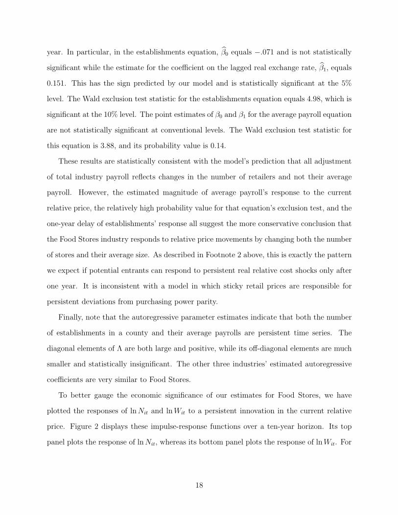
year. In particular, in the establishments equation, β̂0 equals −.071 and is not statistically
significant while the estimate for the coefficient on the lagged real exchange rate, β̂1, equals
0.151. This has the sign predicted by our model and is statistically significant at the 5%
level. The Wald exclusion test statistic for the establishments equation equals 4.98, which is
significant at the 10% level. The point estimates of β0 and β1 for the average payroll equation
are not statistically significant at conventional levels. The Wald exclusion test statistic for
this equation is 3.88, and its probability value is 0.14.
These results are statistically consistent with the model’s prediction that all adjustment
of total industry payroll reflects changes in the number of retailers and not their average
payroll. However, the estimated magnitude of average payroll’s response to the current
relative price, the relatively high probability value for that equation’s exclusion test, and the
one-year delay of establishments’ response all suggest the more conservative conclusion that
the Food Stores industry responds to relative price movements by changing both the number
of stores and their average size. As described in Footnote 2 above, this is exactly the pattern
we expect if potential entrants can respond to persistent real relative cost shocks only after
one year. It is inconsistent with a model in which sticky retail prices are responsible for
persistent deviations from purchasing power parity.
Finally, note that the autoregressive parameter estimates indicate that both the number
of establishments in a county and their average payrolls are persistent time series. The
diagonal elements of Λ are both large and positive, while its off-diagonal elements are much
smaller and statistically insignificant. The other three industries’ estimated autoregressive
coefficients are very similar to Food Stores.
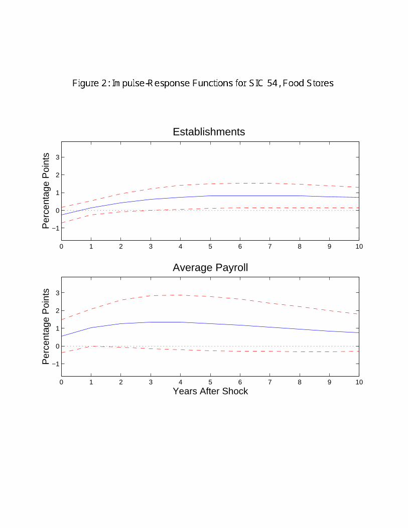
To better gauge the economic significance of our estimates for Food Stores, we have
plotted the responses of lnNit and lnWit to a persistent innovation in the current relative
price. Figure 2 displays these impulse-response functions over a ten-year horizon. Its top
panel plots the response of lnNit, whereas its bottom panel plots the response of lnWit. For
18
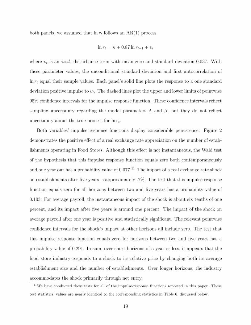
both panels, we assumed that ln rt follows an AR(1) process
ln rt = κ+ 0.87 ln rt−1 + υt
where υt is an i.i.d. disturbance term with mean zero and standard deviation 0.037. With
these parameter values, the unconditional standard deviation and first autocorrelation of
ln rt equal their sample values. Each panel’s solid line plots the response to a one standard
deviation positive impulse to υt. The dashed lines plot the upper and lower limits of pointwise
95% confidence intervals for the impulse response function. These confidence intervals reflect
sampling uncertainty regarding the model parameters Λ and β, but they do not reflect
uncertainty about the true process for ln rt.
Both variables’ impulse response functions display considerable persistence. Figure 2
demonstrates the positive effect of a real exchange rate appreciation on the number of estab-
lishments operating in Food Stores. Although this effect is not instantaneous, the Wald test
of the hypothesis that this impulse response function equals zero both contemporaneously
and one year out has a probability value of 0.077.11 The impact of a real exchange rate shock
on establishments after five years is approximately .7%. The test that this impulse response
function equals zero for all horizons between two and five years has a probability value of
0.103. For average payroll, the instantaneous impact of the shock is about six tenths of one
percent, and its impact after five years is around one percent. The impact of the shock on
average payroll after one year is positive and statistically significant. The relevant pointwise
confidence intervals for the shock’s impact at other horizons all include zero. The test that
this impulse response function equals zero for horizons between two and five years has a
probability value of 0.291. In sum, over short horizons of a year or less, it appears that the
food store industry responds to a shock to its relative price by changing both its average
establishment size and the number of establishments. Over longer horizons, the industry
accommodates the shock primarily through net entry.11We have conducted these tests for all of the impulse-response functions reported in this paper. These
test statistics’ values are nearly identical to the corresponding statistics in Table 6, discussed below.
19
B Other Industries
Table 6 reports the estimates of β and the exclusion tests for all four of the industries we
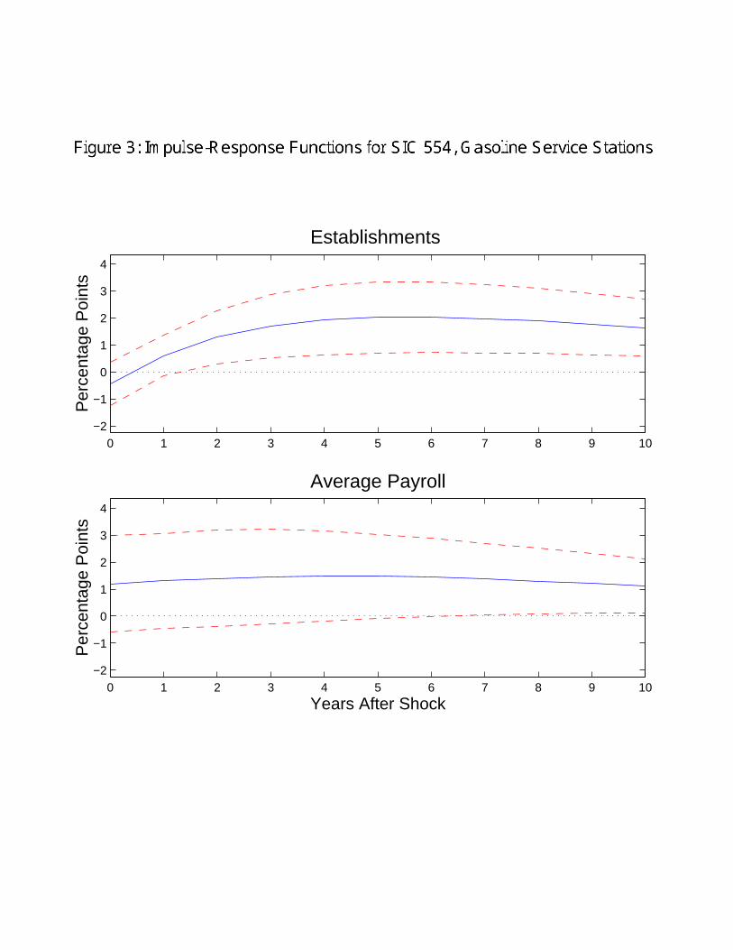
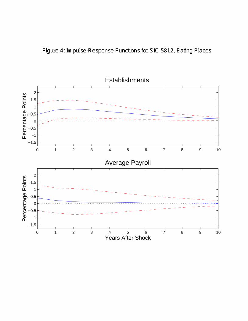
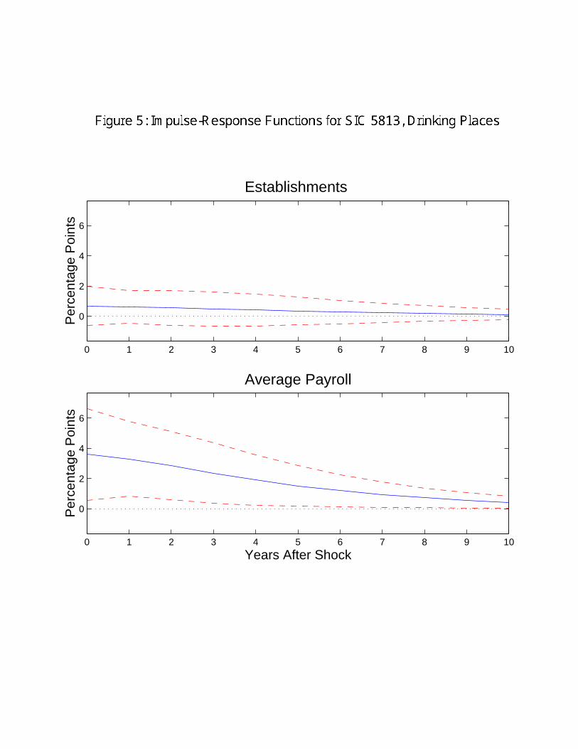
consider, and Figures 3, 4, and 5 graph their impulse response functions. Just as with Food
Stores, the responses in these figures are to a persistent real exchange rate shock from a
first-order autoregression parameterized to match the reported statistics in Table 4.
The results for Gasoline Service Stations are very similar to those for Food Stores. In
particular, the lagged gasoline-based real exchange rate has a positive and statistically sig-
nificant coefficient while the coefficient on the current relative price is insignificant. Thus, in
this industry the number of establishments responds to real exchange-rate shocks after one
year. The Wald test rejects the exclusion restriction for establishments at the 5% level, but
not for average payroll. However, the Wald test statistic for the average payroll equation is
not very small; so it is premature to conclude that Gasoline Service Stations’ average payroll
does not respond to real exchange rate shocks. The impulse-response functions for Gasoline
Service Stations reflect the delayed response of net entry to the exchange rate shock. In
the year of the shock, average payroll rises more than 1%, while the number of establish-
ments falls very slightly. Thereafter, the increase in average payroll persists as the number
of establishments rises. After five years, the number of establishments has increased by
approximately 2%.
Of the four industries we consider, Eating Places most resembles the stark behavior of our
model with immediate entry. Although neither of the coefficients on the real exchange rate
are individually significant in the establishments equation, the Wald test’s probability value
is relatively low, 0.025. The corresponding Wald test statistic for the average payroll equation
is very small. The impulse response functions for Eating Places show that fluctuations in
the number of establishments play a central role in the responses to real exchange rate
disturbances. The contemporaneous responses of establishments and average payroll to the
exchange rate shock are nearly equal. After impact, average payroll quickly returns to its
pre-shock value, while the number of establishments persists at its higher level.
20
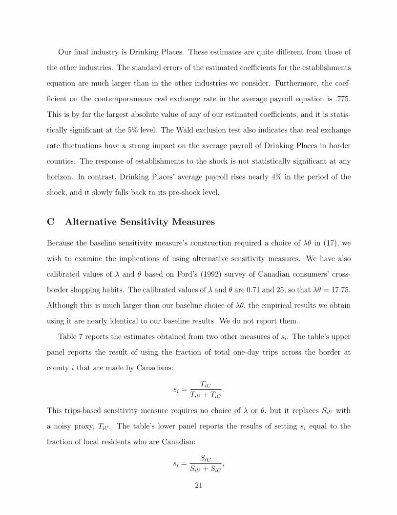
Our final industry is Drinking Places. These estimates are quite different from those of
the other industries. The standard errors of the estimated coefficients for the establishments
equation are much larger than in the other industries we consider. Furthermore, the coef-
ficient on the contemporaneous real exchange rate in the average payroll equation is .775.
This is by far the largest absolute value of any of our estimated coefficients, and it is statis-
tically significant at the 5% level. The Wald exclusion test also indicates that real exchange
rate fluctuations have a strong impact on the average payroll of Drinking Places in border
counties. The response of establishments to the shock is not statistically significant at any
horizon. In contrast, Drinking Places’ average payroll rises nearly 4% in the period of the
shock, and it slowly falls back to its pre-shock level.
C Alternative Sensitivity Measures
Because the baseline sensitivity measure’s construction required a choice of λθ in (17), we
wish to examine the implications of using alternative sensitivity measures. We have also
calibrated values of λ and θ based on Ford’s (1992) survey of Canadian consumers’ cross-
border shopping habits. The calibrated values of λ and θ are 0.71 and 25, so that λθ = 17.75.
Although this is much larger than our baseline choice of λθ, the empirical results we obtain
using it are nearly identical to our baseline results. We do not report them.
Table 7 reports the estimates obtained from two other measures of si. The table’s upper
panel reports the result of using the fraction of total one-day trips across the border at
county i that are made by Canadians:
si =TiC
TiU + TiC.
This trips-based sensitivity measure requires no choice of λ or θ, but it replaces SiU with
a noisy proxy, TiU . The table’s lower panel reports the results of setting si equal to the
fraction of local residents who are Canadian:
si =SiC
SiU + SiC,
21

where SiC is measured using Canada’s 1991 census as the number of Canadians living within
fifty miles of county i’s central point, as defined by the U.S. Census. As we noted above
in Section II, this population-based measure takes no account of the potential difficulties in
travelling between these Canadians homes and county i.
In spite of these potential shortcomings, the results from these two alternative measures
of si are very similar to each other and to our baseline measure. The point estimates from
using the trips-based sensitivity measure are nearly identical to our baseline estimates, and
the pattern of inference is also similar to that based on the test statistics in Table 6. The
point estimates from using the population-based sensitivity measure are also very similar to
those in Table 6, but the pattern of inference changes more. Overall, these alternative sensi-
tivity measures do not substantially alter the conclusion that establishments in Food Stores,
Gasoline Service Stations, and Eating Places, respond within one year to real exchange rate
disturbances.12
D OLS Estimation
To gain a sense of how our results depend on our GMM estimation procedure, Table 8
reports results from estimating a version of our model using ordinary least squares. These
estimates are only consistent as the number of time periods in the sample becomes large
for a fixed number of counties, an assumption that poorly characterizes our sample of 256
counties over 20 years. Nevertheless, the estimated coefficients on the real exchange rate are
very similar to those reported in Table 6. The estimated standard errors are comparable
to those from the GMM estimation, and inference based on their exclusion tests is similar
to that using the GMM based tests. However, the exclusion test’s probability value rises
to 0.138 for the coefficients in Eating Places’ establishments equation while it falls to 0.03812We have also estimated our model using a sensitivity measure that simply equals one if the county is
on the U.S.-Canada border and equals zero otherwise. The results from this estimation are also similar to
those from the baseline estimation.
22

for those in Gasoline Service Stations’ average payroll equation. It appears that our results
manifest themselves even in a simple OLS regression.
IV Related Literature
This paper’s analysis of the effects of border residents’ arbitrage opportunities and their
effects on retail trade industries is related to the literature in international economics which
focuses on the degree of goods’ market segmentation. Engel and Rogers (1996) examine
relative consumer-level prices between U.S. and Canadian cities and conclude that U.S. and
Canadian markets are segmented to a greater extent than can be explained by distance,
formal trade restrictions, or sticky nominal prices. Our findings that movements in real ex-
change rates have real effects on U.S. industries located near the border strongly suggest that
these price differences extend right up to the U.S.-Canada border and so characterize nearly
identical goods that are sold only a short distance apart. These observations reinforce Engel
and Roger’s conclusion that U.S. and Canadian goods markets are not well integrated and
suggests that international segmentation characterizes other markets such as input markets
for labor, wholesale goods, and distribution networks.
Our results are also related to the branch of international macroeconomics which fo-
cuses on the puzzle of persistent deviations from PPP and the related observation that
consumer prices are not very responsive to nominal exchange rate movements. Obstfeld
and Rogoff (2000) examine environments in which nominal prices are fixed in producers’
currencies (producer currency pricing) while Betts and Devereux (2000) and Chari, Kehoe,
and McGrattan (2000b) present models in which sticky nominal prices are denominated in
the currency of consumers (local currency pricing). Devereux and Engel (2000) and Engel
(2001) demonstrate that these two classes of models have very different implications for the
degree of optimal exchange rate flexibility. Our finding that the expenditure-shifting effects
of exchange rates impact the number of operating establishments in Food Stores, Gasoline
23
Service Stations, and Eating Places is inconsistent with the view that stickiness in retail-
ers’ nominal prices is a central cause of persistent deviations from PPP. Our results do not
directly support the assumption of producer currency pricing, but they do eliminate one oth-
erwise promising source of sticky local currency pricing, retailers. This places responsibility
for any nominal price stickiness upstream to either wholesalers, manufacturers, or as in the
case of gasoline in the early 1980’s, regulators.
Much of the theory of industrial organization assumes that entry responds to persistent
shocks only in the long run, so that incumbent producers can temporarily earn economic
profits following a favorable aggregate demand or cost shock. Baumol, Panzar, and Willig
(1982) show that the opposite assumption of very rapid entry with no sunk costs implies
that incumbents never earn positive profits and that price always equals average cost. In
spite of this theoretical importance, little is known about the speed with which entry can
take place following a demand shock. Only in Drinking Places, where alcohol licensing
restrictions might present a barrier to entry, does the real exchange rate affect industry
activity without changing the number of establishments. In the other three industries we
consider, either potential entrants, potential exiters, or both must respond relatively rapidly
to demand shocks. In our model economy and its extension discussed in Footnote 1 that
incorporates sunk costs of entry and long-lived producers, all fluctuations in the number of
producers reflect the decisions of potential entrants rather than exiting incumbents. This is
a very robust theoretical result that only depends on the cost of entry being invariant to the
number of entrants and their identities.13 Thus, our results strongly suggest that potential
entrants can affect their decisions shortly after demand shocks.13Campbell and Fisher (1996) present a perfectly competitive industry dynamics model with idiosyncratic
producer risk, sunk costs of entry, and endogenous exit. In that model, demand shocks only contemporane-
ously impact the number of entrants.
24
V Conclusion
Blinder (1993) asserts that the various microeconomic explanations for individual producers’
nominal rigidities are intrinsically untestable because they only generate the single prediction
of infrequent price adjustment. Rather than examining the implications of these theories,
this paper examines their common prerequisite of a stable industry structure over the short
run. For three of the four retail trade industries we examine, the data favors a model in
which potential producers’ entry decisions respond relatively quickly to the real and nominal
disturbances underlying fluctuations in the real exchange rate. The massive, ongoing, and
cyclically sensitive restructuring of employment in the manufacturing sector documented by
Davis, Haltiwanger, and Schuh (1996) suggests that this critique of sticky price models may
be applicable far beyond the four retail trade industries we consider. For this reason, we
believe that a more general examination of the comovement of net entry with real exchange
rates is a promising avenue for future research into the source of nominal price rigidities.
Our results cast doubt on theories of sluggish individual price adjustment based on pro-
ducers’ costs of changing nominal prices, but the observations that individual producers
change their prices infrequently and that their price changes are not highly correlated, made
for example by Carlton (1986) and Lach and Tsiddon (1996), remain. The observation of in-
frequent price adjustment does not immediately imply that producers face nominal rigidities.
For example, Eden (1994) demonstrates that infrequent discrete jumps in nominal prices are
also consistent with an uncertain and sequential trading (UST) model in which sellers are
indifferent among a large range of real prices. In that environment, one optimal pricing pol-
icy is to change a nominal price only when inflationary pressures causes the corresponding
real price to move out of that range. Eden (2001) argues that observed price adjustment
patterns in Lach and Tsiddon’s (1996) data are inconsistent with an environment based on
nominal rigidities but are consistent with a simple UST model. Our results reinforce this
conclusion and suggest that the informational frictions underpinning the UST model may
be quite important for the retail trade industries we consider.
25
References
Baumol, William J., John C. Panzar, and Robert D. Willig. (1982) Contestable Markets and
the Theory of Industry Structure. New York, Harcourt Brace Jovanovich.
Betts, Caroline and Michael Devereux. (2000) Exchange Rate Dynamics in a Model of
Pricing-to-Market. Journal of International Economics 50, 215-244.
Blinder, Alan S. (1993) Why Are Prices Sticky? Preliminary Results from an Interview
Study, in Optimal Pricing, Inflation, and the Cost of Price Adjustment, Eytan Sheshinski
and Yoram Weiss, eds., MIT Press, Cambridge, MA.
Blundell, Richard and Stephen Bond. (1998) Initial Conditions and Moment Restrictions in
Dynamic Panel Data Models. Journal of Econometrics, 87(1), 115–143.
Campbell, Jeffrey R. and Jonas D.M. Fisher. (1996) Aggregate Employment Fluctuations
with Microeconomic Asymmetries. NBER Working Paper 5767.
Carlton, Dennis W. (1986) The Rigidity of Prices. American Economic Review, 76(4),
637–658.
Chari, V.V., Patrick J. Kehoe, and Ellen R. McGrattan. (2000a) Sticky Price Models of the
Business Cycle: Can the Contract Multiplier Solve the Persistence Problem? Econometrica,
68(5), 1151–1179.
Chari, V.V., Patrick J. Kehoe, and Ellen R. McGrattan. (2000b) Can Sticky Price Models
Generate Volatile and Persistent Real Exchange Rates? Federal Reserve Bank of Minneapolis
Research Department Staff Report 277.
Christiano, Lawrence J., Martin Eichenbaum, and Charles Evans. (2001) Nominal Rigidities
and the Dynamic Effects of a Shock to Monetary Policy. NBER Working Paper 8403.
Davis, Steven J., John C. Haltiwanger, and Scott Schuh. (1996) Job Creation and Destruc-
tion, MIT Press, Cambridge, MA.
26
Devereux, Michael B. and Charles Engel. (2000) Monetary Policy in the Open Economy
Revisited: Price Setting and Exchange Rate Flexibility. NBER Working Paper 7665.
Eden, Benjamin. (1994) The Adjustment of Prices to Monetary Shocks when Trading is
Uncertain and Sequential. Journal of Political Economy, 102(3), 493–509.
Eden, Benjamin. (2001) Inflation and Price Adjustment: An Analysis of Micro Data. Review
of Economic Dynamics, 4(3), 607–636.
Engel, Charles and John Rogers. (1996) How Wide is the Border? American Economic
Review, 86(5), 1112-1125.
Engel, Charles. (2001) The Responsiveness of Consumer Prices to Exchange Rates and
the Implications for Exchange-Rate Policy: A Survey of a few Recent New Open-Economy
Macro Models. Working Paper, University of Wisconsin.
Ford, Theresa. (1992) International Outshopping Along the Canada-United States Border:
The Case of Western New York. Canada-United States Trade Center Occasional Paper No.
12, State University of New York at Buffalo
Foster, Lucia, John Haltiwanger, and C.J. Krizan. (2001) The Link Between Aggregate and
Micro Productivity Growth: Evidence from Retail Trade. Working Paper, University of
Maryland.
Lach, Saul and Daniel Tsiddon. (1996) Staggering and Synchronization in Price-Setting:
Evidence from Multiproduct Firms. American Economic Review, 86(5), 1175–1196.
MacDonald, James M. and Daniel Aaronson. (2000) How Do Retail Prices React to Mini-
mum Wage Increases? Federal Reserve Bank of Chicago Working Paper 00-20.
Obstfeld, Maurice and Kenneth Rogoff. (2000) New Directions for Stochastic Open Economy
Models. Journal of International Economics, 50(1), 117–153.
27
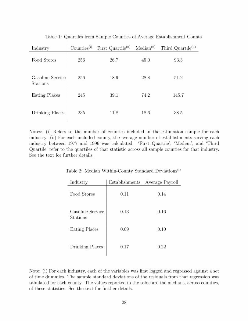
Table 1: Quartiles from Sample Counties of Average Establishment Counts
Industry Counties(i) First Quartile(ii) Median(ii) Third Quartile(ii)
Food Stores 256 26.7 45.0 93.3
Gasoline Service 256 18.9 28.8 51.2Stations
Eating Places 245 39.1 74.2 145.7
Drinking Places 235 11.8 18.6 38.5
Notes: (i) Refers to the number of counties included in the estimation sample for eachindustry. (ii) For each included county, the average number of establishments serving eachindustry between 1977 and 1996 was calculated. ‘First Quartile’, ‘Median’, and ‘ThirdQuartile’ refer to the quartiles of that statistic across all sample counties for that industry.See the text for further details.
Table 2: Median Within-County Standard Deviations(i)
Industry Establishments Average Payroll
Food Stores 0.11 0.14
Gasoline Service 0.13 0.16Stations
Eating Places 0.09 0.10
Drinking Places 0.17 0.22
Note: (i) For each industry, each of the variables was first logged and regressed against a setof time dummies. The sample standard deviations of the residuals from that regression wastabulated for each county. The values reported in the table are the medians, across counties,of these statistics. See the text for further details.
28
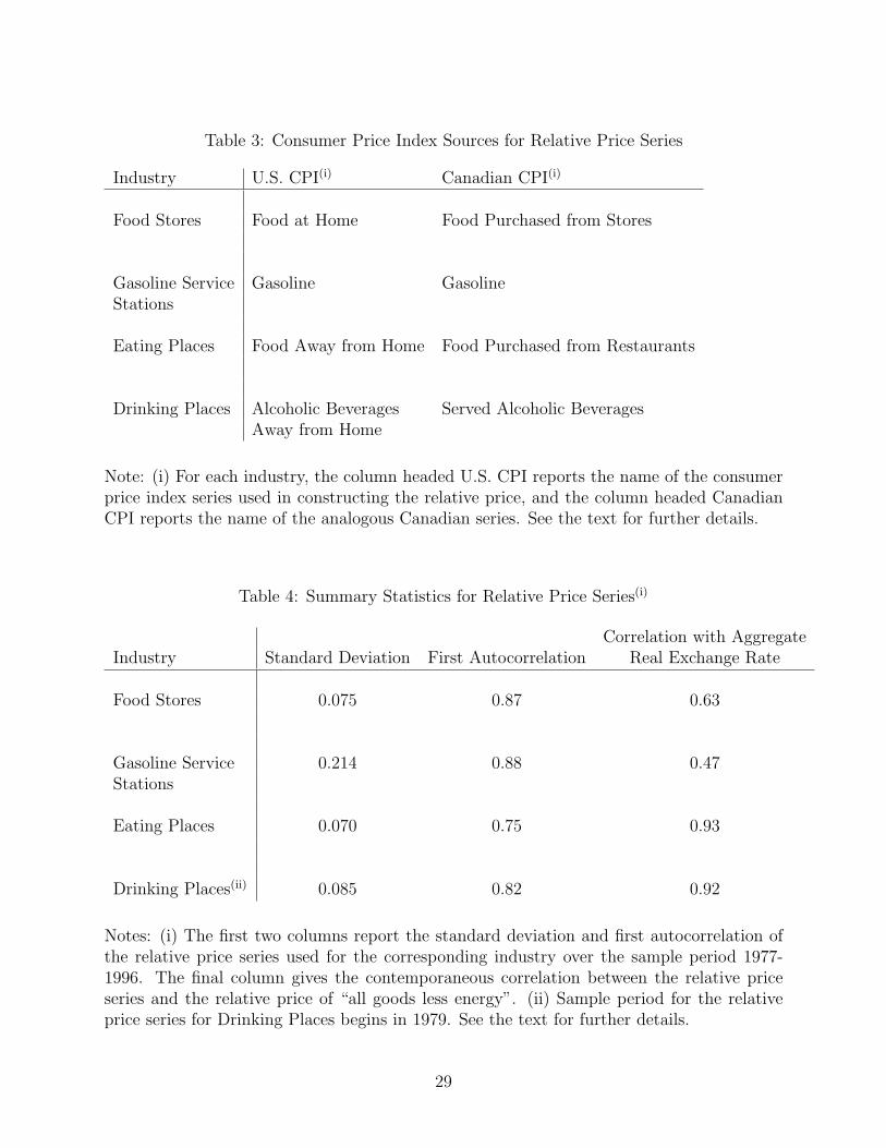
Table 3: Consumer Price Index Sources for Relative Price Series
Industry U.S. CPI(i) Canadian CPI(i)
Food Stores Food at Home Food Purchased from Stores
Gasoline Service Gasoline GasolineStations
Eating Places Food Away from Home Food Purchased from Restaurants
Drinking Places Alcoholic Beverages Served Alcoholic BeveragesAway from Home
Note: (i) For each industry, the column headed U.S. CPI reports the name of the consumerprice index series used in constructing the relative price, and the column headed CanadianCPI reports the name of the analogous Canadian series. See the text for further details.
Table 4: Summary Statistics for Relative Price Series(i)
Correlation with AggregateIndustry Standard Deviation First Autocorrelation Real Exchange Rate
Food Stores 0.075 0.87 0.63
Gasoline Service 0.214 0.88 0.47Stations
Eating Places 0.070 0.75 0.93
Drinking Places(ii) 0.085 0.82 0.92
Notes: (i) The first two columns report the standard deviation and first autocorrelation ofthe relative price series used for the corresponding industry over the sample period 1977-1996. The final column gives the contemporaneous correlation between the relative priceseries and the relative price of “all goods less energy”. (ii) Sample period for the relativeprice series for Drinking Places begins in 1979. See the text for further details.
29
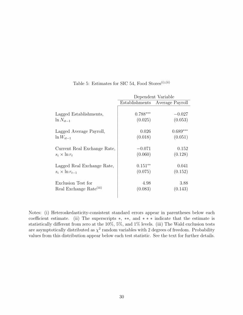
Table 5: Estimates for SIC 54, Food Stores(i),(ii)
Dependent VariableEstablishments Average Payroll
Lagged Establishments, 0.788∗∗∗ −0.027lnNit−1 (0.025) (0.053)
Lagged Average Payroll, 0.026 0.689∗∗∗
lnWit−1 (0.018) (0.051)
Current Real Exchange Rate, −0.071 0.152si × ln rt (0.060) (0.128)
Lagged Real Exchange Rate, 0.151∗∗ 0.041si × ln rt−1 (0.075) (0.152)
Exclusion Test for 4.98 3.88Real Exchange Rate(iii) (0.083) (0.143)
Notes: (i) Heteroskedasticity-consistent standard errors appear in parentheses below eachcoefficient estimate. (ii) The superscripts ∗, ∗∗, and ∗ ∗ ∗ indicate that the estimate isstatistically different from zero at the 10%, 5%, and 1% levels. (iii) The Wald exclusion testsare asymptotically distributed as χ2 random variables with 2 degrees of freedom. Probabilityvalues from this distribution appear below each test statistic. See the text for further details.
30
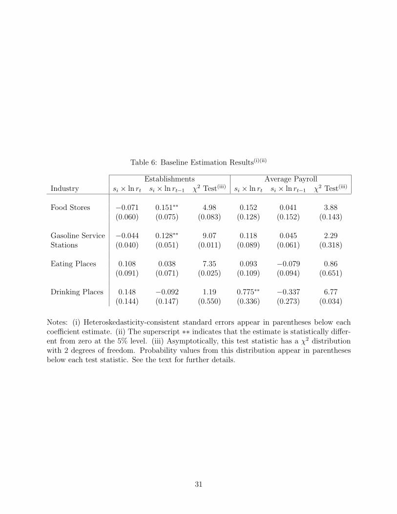
Table 6: Baseline Estimation Results(i)(ii)
Establishments Average PayrollIndustry si × ln rt si × ln rt−1 χ2 Test(iii) si × ln rt si × ln rt−1 χ2 Test(iii)
Food Stores −0.071 0.151∗∗ 4.98 0.152 0.041 3.88(0.060) (0.075) (0.083) (0.128) (0.152) (0.143)
Gasoline Service −0.044 0.128∗∗ 9.07 0.118 0.045 2.29Stations (0.040) (0.051) (0.011) (0.089) (0.061) (0.318)
Eating Places 0.108 0.038 7.35 0.093 −0.079 0.86(0.091) (0.071) (0.025) (0.109) (0.094) (0.651)
Drinking Places 0.148 −0.092 1.19 0.775∗∗ −0.337 6.77(0.144) (0.147) (0.550) (0.336) (0.273) (0.034)
Notes: (i) Heteroskedasticity-consistent standard errors appear in parentheses below eachcoefficient estimate. (ii) The superscript ∗∗ indicates that the estimate is statistically differ-ent from zero at the 5% level. (iii) Asymptotically, this test statistic has a χ2 distributionwith 2 degrees of freedom. Probability values from this distribution appear in parenthesesbelow each test statistic. See the text for further details.
31
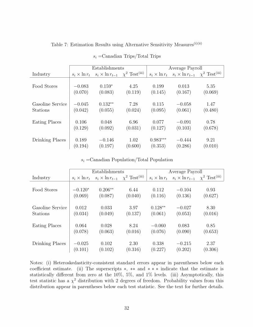
Table 7: Estimation Results using Alternative Sensitivity Measures(i)(ii)
si =Canadian Trips/Total Trips
Establishments Average PayrollIndustry si × ln rt si × ln rt−1 χ2 Test(iii) si × ln rt si × ln rt−1 χ2 Test(iii)
Food Stores −0.083 0.159∗ 4.25 0.199 0.013 5.35(0.070) (0.083) (0.119) (0.145) (0.167) (0.069)
Gasoline Service −0.045 0.132∗∗ 7.28 0.115 −0.058 1.47Stations (0.042) (0.055) (0.024) (0.095) (0.061) (0.480)
Eating Places 0.106 0.048 6.96 0.077 −0.091 0.78(0.129) (0.092) (0.031) (0.127) (0.103) (0.678)
Drinking Places 0.189 −0.146 1.02 0.983∗∗∗ −0.444 9.21(0.194) (0.197) (0.600) (0.353) (0.286) (0.010)
si =Canadian Population/Total Population
Establishments Average PayrollIndustry si × ln rt si × ln rt−1 χ2 Test(iii) si × ln rt si × ln rt−1 χ2 Test(iii)
Food Stores −0.120∗ 0.206∗∗ 6.44 0.112 −0.104 0.93(0.069) (0.087) (0.040) (0.116) (0.136) (0.627)
Gasoline Service 0.012 0.033 3.97 0.128∗∗ −0.027 8.30Stations (0.034) (0.049) (0.137) (0.061) (0.053) (0.016)
Eating Places 0.064 0.028 8.24 −0.060 0.083 0.85(0.078) (0.063) (0.016) (0.076) (0.090) (0.653)
Drinking Places −0.025 0.102 2.30 0.338 −0.215 2.37(0.101) (0.102) (0.316) (0.227) (0.202) (0.306)
Notes: (i) Heteroskedasticity-consistent standard errors appear in parentheses below eachcoefficient estimate. (ii) The superscripts ∗, ∗∗ and ∗ ∗ ∗ indicate that the estimate isstatistically different from zero at the 10%, 5%, and 1% levels. (iii) Asymptotically, thistest statistic has a χ2 distribution with 2 degrees of freedom. Probability values from thisdistribution appear in parentheses below each test statistic. See the text for further details.
32
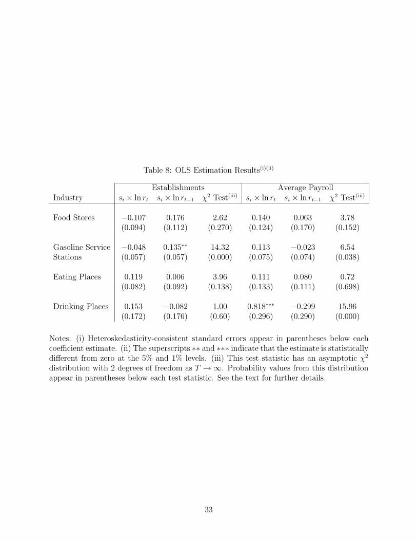
Table 8: OLS Estimation Results(i)(ii)
Establishments Average PayrollIndustry si × ln rt si × ln rt−1 χ2 Test(iii) si × ln rt si × ln rt−1 χ2 Test(iii)
Food Stores −0.107 0.176 2.62 0.140 0.063 3.78(0.094) (0.112) (0.270) (0.124) (0.170) (0.152)
Gasoline Service −0.048 0.135∗∗ 14.32 0.113 −0.023 6.54Stations (0.057) (0.057) (0.000) (0.075) (0.074) (0.038)
Eating Places 0.119 0.006 3.96 0.111 0.080 0.72(0.082) (0.092) (0.138) (0.133) (0.111) (0.698)
Drinking Places 0.153 −0.082 1.00 0.818∗∗∗ −0.299 15.96(0.172) (0.176) (0.60) (0.296) (0.290) (0.000)
Notes: (i) Heteroskedasticity-consistent standard errors appear in parentheses below eachcoefficient estimate. (ii) The superscripts ∗∗ and ∗∗∗ indicate that the estimate is statisticallydifferent from zero at the 5% and 1% levels. (iii) This test statistic has an asymptotic χ2
distribution with 2 degrees of freedom as T →∞. Probability values from this distributionappear in parentheses below each test statistic. See the text for further details.
33
1972
1976
1980
1984
1988
1992
1996
68
10
12
14
1972
1976
1980
1984
1988
1992
1996
8
10
12
14
16
18
20
22
24
26
28
30
1972
1976
1980
1984
1988
1992
1996
.7
.75
.8
.85
.9
.951
Yea
r
U.S. Same-Day Trips(Millions)
Canadian Same-Day Trips(Millions)
Real Exchange Rate(1772=1)
0 1 2 3 4 5 6 7 8 9 10
−1
0
1
2
3
Establishments
Per
cent
age
Poi
nts
0 1 2 3 4 5 6 7 8 9 10
−1
0
1
2
3
Average Payroll
Per
cent
age
Poi
nts
Years After Shock
0 1 2 3 4 5 6 7 8 9 10−2
−1
0
1
2
3
4
Establishments
Per
cent
age
Poi
nts
0 1 2 3 4 5 6 7 8 9 10−2
−1
0
1
2
3
4
Average Payroll
Per
cent
age
Poi
nts
Years After Shock
0 1 2 3 4 5 6 7 8 9 10
−1.5
−1
−0.5
0
0.5
1
1.5
2
Establishments
Per
cent
age
Poi
nts
0 1 2 3 4 5 6 7 8 9 10
−1.5
−1
−0.5
0
0.5
1
1.5
2
Average Payroll
Per
cent
age
Poi
nts
Years After Shock
0 1 2 3 4 5 6 7 8 9 10
0
2
4
6
Establishments
Per
cent
age
Poi
nts
0 1 2 3 4 5 6 7 8 9 10
0
2
4
6
Average Payroll
Per
cent
age
Poi
nts
Years After Shock