1

Abstract—Industrial process monitoring and modelling represents a critical step in order to achieve the paradigm of Zero Defect Manufacturing. The aim of this paper is to introduce the Neo-Fuzzy Neuron method to be applied in industrial time series modelling. Its open structure and input independency provides fast learning and convergence capabilities, while assuring a proper accuracy and generalization in the modelled output. First, the auxiliary signals in the database are analyzed in order to find correlations with the target signal. Second, the Neo-Fuzzy Neuron is configured and trained according by means of the auxiliary signal, past instants and dynamics information of the target signal. The proposed method is validated by means of real data from a Spanish copper rod industrial plant, in which a critical signal regarding copper refrigeration process is modelled. The obtained results indicate the suitability of the Neo-Fuzzy Neuron method for industrial process modelling. 1

Index Terms— Artificial intelligence, Forecasting, Fuzzy neural networks, Industrial plants, Predictive models, Time series analysis.

I. INTRODUCTION

NDUSTRY 4.0 is a trend keyword in the industrial environment that aims to match productive processes with

the new information and communication technologies [1]. It is the path for industries to achieve the paradigm of the Factory of the Future. Therefore, Industry 4.0 is seen as coherent aggrupation of new emerging technologies such as the Wireless Sensor Networks (WSN) [2], Internet of Things (IoT) [3]-[4], Cyber Physical Systems (CPS) [5], Big Data analytics (BD) [6]- [7], process optimization [8], support to human [8]-[9], among others, that work together to maximize plant performance and resources [11]-[12].

The basis for the deployment of such technologies relies on data management. Indeed, the analysis and the exploitation of plant data is a critical step in order to achieve the objectives of Zero Defect Manufacturing (ZDM) [13]. ZDM is a framework aligned in the Industry 4.0 and represents the ideal goal for an industrial plant to produce without any defect [14]. It assumes that the quality of a product is totally associated to the proper functioning of the different processes involved in its fabrication. If all of them are in perfect condition, the final

This research was supported in part by the Spanish Ministry of Education, Culture, and Sport under the grant FPU13/00589. The authors also wish to acknowledge financial support from the Generalitat de Catalunya (GRC MCIA, Grant nº SGR 2014-101).

product’s quality must be optimal. Consequently, the problem turns to the proper monitoring and modelling of the plant critical processes and signals [15].

In this regard, there are basically three different approaches to conduct modelling: (i) physical modelling, (ii) probabilistic modelling and (iii) data-driven modelling [16]-[17]. Due to the complex nature of industrial processes both physical and probabilistic methods present many limitations in terms of: computational cost and generalization, for the physical approach, and a lack of precision and adaptability to the probabilistic ones [18]. On the other hand, technology improvements in the field of sensing and instrumentation is leading industries into rich data environments, in which data regarding different parts of the process is acquired and systematically stored in a database.

Classically, data-driven modelling approaches were faced by the application of the Neural Networks (NN) [19], or the Adaptive Neuro Fuzzy Inference Systems (ANFIS) [20]. Indeed, all data-driven approaches demand an intensive data comprehension. In this regard, the high approximation capability of ANFIS is due to its ability to adapt the Membership Functions (MF) of the input layer by considering the interrelation between the inputs and the target. This crucial step can be seen as a signal selection layer that aims to consider the most valuable information and discard those inputs that do not affect the target [21]. However, this particularization of the model requires high amount of data, slows the convergence of the solution and masks the relations between the inputs and the target. This selection procedure turns into a limitation when the model needs to address a high amount of inputs, as is the case of industrial time series.

In this context, the Neo-Fuzzy Neuron (NFN) is a modelling method that offers interesting capabilities to be exploded in the industrial field. It presents an open and modular architecture that generates a dedicated modelling unit for each input that is introduced to the model [22]. Then, the inputs are connected in a collaborative way to give the final outcome. In this structure, the relation of the inputs with the target can be easily identified, this leads to higher solution convergence ratio, which implies

D. Zurita, M. Delgado, J.A. Carino, and J.A. Ortega, are with the MCIA Research Center, Department of Electronic Engineering, Technical University of Catalonia (UPC), Terrassa, 08222, Spain. E-mail: [daniel.zurita, miguel.delgado, jesus.carino, juan.antonio.ortega] @mcia.upc.edu.

G. Clerc, is with the Laboratoire Ampère, Université Lyon 1, Villeurbanne, France; CNRS, UMR 5005. E-mail: guy.clerc@univ-lyon1.fr.

Daniel Zurita, Student Member, IEEE, Miguel Delgado, Member, IEEE, Jesus A. Carino, Student Member, IEEE, Juan A. Ortega, Member, IEEE, Guy Clerc, Senior Member, IEEE

Industrial Time Series Modelling by means of the Neo-Fuzzy Neuron

I

2

lower data requirements and fewer training iterations, this results in a less overfitted approach [26]-[27]. Therefore, the NFN together with a simply correlation study in order to assure the utility of the selected model inputs offers a reliable and accurate solution for industrial process modelling.

In this paper, the NFN method is proposed for industrial time series modelling. First, auxiliary signals of the database are analyzed by means of a correlation analysis to detect the appropriate set of inputs to the model. Then, the NFN is configured and trained to learn the behavior of the target signal. Finally the proposed method is compared in terms of performance with a classic ANFIS approach. Note that is the first time that NFN method is applied in industrial applications.

This paper is organized as follows: Section II introduces the concepts behind industrial time series modelling. In Section III, the basis of the NFN architecture are explained. Section IV presents the industrial plant used for testing the suitability of the method and the analysis of such data. Finally, in Section V, the experimental results and the method capabilities are verified.

II. INDUSTRIAL TIME SERIES MODELLING

Nowadays, industrial time series modelling represents an area of growing interest for many researchers due to the convergence of industry and new information technologies. Indeed, it is a novel field of study and most of the works found in literature are focused on presenting generic frameworks or solving specific applications. As previous works, J. Lee et al. [25], propose to use autoregressive moving average (ARMA) together with match matrix methods to generate a watchdog agent to model critical parts of the process and track their condition. O. Myklebust [26], proposes a ZDM framework with focuses on maintenance, in which a combination of data-driven models are able to detect early indication of abnormal behavior or wear of manufacturing processes. J. Lee et al. [27], proposes a framework for a predictive manufacturing system based in CPSs, which are models or “virtual twins” of the real machines and are used to model and forecast process condition. Despite the lack of a standard methodology for facing the modelling, common aspects and issues to be faced can be identified in such literature. Therefore, such aspects should be remarked as the characteristic properties of industrial time series and be considered for any approach.

One of the most critical aspects to consider is the forecasting horizon. This parameter fixes the time step that the model should infer in the future, and it is critical as it directly conditions model performance and viability. The forecasting horizon can be either fixed by the application, if information for a specific future step is required [28], or optimized to reach the furthest horizon the model could give in regard with available information [29]. In this respect, industrial time series present a characteristic non-periodic and complex behavior that causes a quick drop of performance as horizon is extended. This is due to the fact that they are affected by the surrounding auxiliary signals and their own dynamics content. Hence, the modelling of such signals involves a combined scenario with two more critical aspects to consider: (i) auxiliary data management, that is to exploit the relations of the auxiliary signals and the targets to increase modelling performance and generalization, and (ii)

signal dynamics analysis, that is to analyze trends and dynamics modes of the signal and include this information in the model to improve accuracy and precision of modelling.

Regarding auxiliary data management, further research has been made in the load forecasting field. In these applications, the signal to model present lower dynamics and a more periodic approach than the industrial ones, but are also very influenced by the auxiliary signals of the process. Therefore, in this field the efforts are concentrated on selecting the best auxiliary inputs for a specific model to improve the performance. Z. Hu et al. [30], propose a hybrid filter-wrapper to select the best inputs for a Support Vector Machine (SVM). F. Keynia [31], presents a mutual information based feature selection method in which the most relevant features are ranked regarding their information addition to the forecasting process, the final modelling is faced by means of a composite NN. K. Kampouropoulos et al. [32], use a Genetic Algorithm (GA) based optimization in order to select the best inputs for an ANFIS based modelling, inputs are treated as chromosomes for the GA algorithm, best combination is given by optimizing the Root Mean Squared Error (RMSE) of the modelling. The main issue behind using input selection methods for auxiliary data management is the difficulty from many modelling methods to handle a considerable number of inputs. Normally, model complexity and overfitting increases with the number of inputs, and also, the number of data required for a proper training increases [33]. So the model is optimized by limiting the number of inputs to the best set filtering signals that does not give additional information for a process, or auxiliary information that is not somehow related with the target [34].

By contrast, other data managing approaches aims to combine, rather than select, the information given by the auxiliary signals in order to reduce the number of inputs. F. M. Bianchi et al. [35], uses Principal Component Analysis (PCA) to compress auxiliary information and uses an Echo-State Network to model the evolution of the signal. C. Brighenti et al. [36], uses the topology preservation properties of Self-Organizing Maps (SOM) in order to analyze industrial process variations in the SOM clusters and its affectation to the critical signal to be modeled. C.W. Frey [37], presents a SOM based schema with watershed transformations to detect different operating areas of an industrial automation network to monitor process changes and deviations. M. Dominguez et al. [38], uses also SOM based compression to monitor operating areas of an industrial process with the aim to detect abnormal behaviors.

It should be pointed that most modelling approaches include information regarding past inputs of the target as auxiliary inputs. However, best past inputs for a defined forecasting horizon must be selected, this procedure is faced primarily by using optimization methods (GA) or correlation analysis [39].

Regarding signal dynamics analysis, most common approaches found in literature are based on the segmentation of different dynamic modes of the signal and the generation of a dedicated model [40]. In this regard, it is very extended the use of Empirical Mode Decomposition (EMD), Z. Guo et al. [41], uses EMD to decompose a chaotic wind signal in dynamic details, then models each detail by a dedicated ANN. W. Wang et al. [42], states that Ensemble Empirical Mode Decomposition (EEMD) offers more results since suppress processes background noise and isolate better the dynamic

3

modes of the signal. J. Eynard et al. [43], proposes to use Wavelet analysis to extract information regarding frequency domain of the target signal while preserving the temporal waveform, then this information was included in a ANN based model to improve the modelling of an industrial process temperature. However, information regarding signal dynamics can be also exploited by means of feature calculations approaches, information regarding the mean value in a time window, or the calculation of the slope from a linear regression are simple approaches to extract dynamic information from the signal and enhance model performance without increasing the computational complexity.

The last concern to face is the modelling method employed, in this regard many research efforts have been made in the use of data-driven methods for modelling industrial time series. A. Zamaniyan et al. [44], uses an optimal configured 3-layer ANN to model the temperature in a hydrogen plant. E. Ceperic, et al. [45], proposes the use of Support Vector Regressions (SVR) together with GA for short-term modelling of industrial consumption signals. L. Dezhi et al. [46], proposes a fuzzy neural network to improve the classic NN in modelling, the authors remarks that adding the fuzzy layer results in an increase of performance and provide more generalization capabilities towards different datasets. Moving to the neuro-fuzzy concept, M.V.V.N. Sriram et al. [20], uses a ANFIS based modelling approach for forecasting the temperature and other parameters from an industrial oxygen furnace, and states that neuro-fuzzy approaches achieve more accurate modelling results than ANN. B. Dehkordi et al. [47], proposes the use of ANFIS for modelling the performance of an electric arc furnace.

Previous research works have been made with NFN. Accordingly, K.T. Chaturvedi et al. [48], proposes the application of NFN for modelling the evolution of economic and power time series. Y. Bodyanskiy et al. [49], uses the NFN for modelling time series properties focusing on chaotic non-linear signals. A. Soualhi et al. [50], proposes the NFN a bearing condition monitoring. In this regard, the main advantages of NFN method are a high learning rate with a limited database, computational simplicity, easy input handling, and the avoiding of overfitting in the output [50].

As a conclusion, the procedure to develop ITS models can be divided in four different steps: (i) Data Pre-Analysis. This step deals with the correlation analysis of auxiliary data to select the most suitable inputs to be introduced to the model. (ii) Model Design. In this step, the internal structure of the model should be fixed, which concerns to the number of inputs, the delayed samples and the auxiliary information. (iii) Model Training. In this step, the input data is prepared and the model is trained with the configured learning algorithm. (iv) Performance Evaluation. Deals with the calculation of performance metrics with the model output in order to evaluate the goodness of the model.

III. NEO-FUZZY NEURON MODELLING

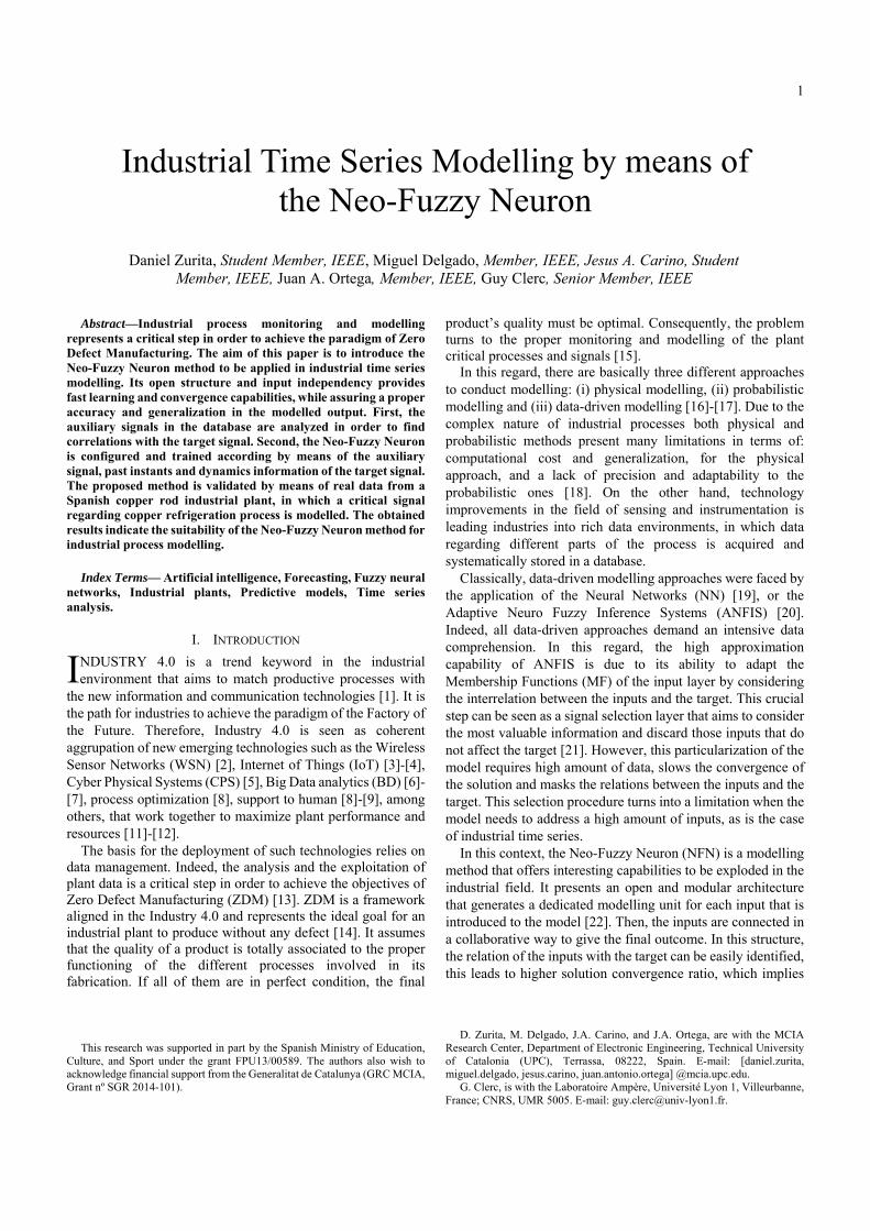
The Neo-Fuzzy Neuron is a nonlinear multi-input single output modelling architecture that was introduced by T. Yamakawa et. al. in [51]–[53]. The structure of a single output, n inputs NFN can be seen in Fig. 1.

 Fig. 1. Neo-Fuzzy Neuron structure. It represents a network with n=3 inputs, and h=3 MF to cover each input.

Let xi be the i-th input, and the predicted output at a predefined forecasting horizon p. In this regard, the output of the NFN is calculated by applying Eq. (1).

  (1) 

The structural modelling units of the NFN are n non-linear synapses, SYi, that connect the inputs of the model with the output by means of , as shown in Eq. (2).

, ,   (2) 

where ωj,i represents the interconnecting weights, and µj,i (xi) represents the membership degree of the i-th input over j-th MF calculated by Eq. (3), where h denotes the number of MF to fuzzify each input.

,

, ,∈ , , ,

,

, ,∈ , , ,

0

  (3) 

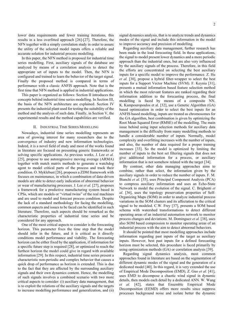
In this regard, all MF of the NFN are triangular functions obtained after the normalization of the input variables as 0 1 . Note that the triangular MF are placed equidistantly with a constant overlapping in the [0- 1] interval, as seen in Fig. 2. Finally, the output value of the synapse is given by Eq. (4). It should be noticed that h should be set in regard with the application, h must be increased in regard with target signal complexity.

, , , ,   (4) 

4

 Fig. 2. Triangular MF that are used for input fuzzification. In the figure, h=5 MF are shown.

The training is the procedure to adapt the h x n synaptic weights of the network. In this regard, NFN uses the Stepwise Training as a learning algorithm to incrementally update the weights of each neuron. For a specific time instant, t, the cost function for the training is defined as the quadratic error of the model output defined in Eq. (5).

12 ⋯

12 , 1 ,

(5) 

Thus, the learning phase turns into a minimization problem that aims to find the optimal weight configuration by means of the gradient descendent method (Backpropagation) [54]. The weights are updated iteratively through the configured training iterations by following Eq. (6), where α is the learning rate of the algorithm that determines the convergence speed.

, 1 ,

, (6) 

Once the model is properly trained, standard statistic metrics can be used in order to evaluate the performance and the accuracy of the NFN model. The most used metrics in the literature are the Root Mean Squared Error (RMSE), the Mean Absolute Error (MAE) and the Mean Absolute Percentage Error (MAPE) [55], which are defined in Eq.(7) to (9), where L is the total length of the signal.

∑

 (7) 

   

∑

  (8) 

   

∑

100% 

(9) 

The use of RMSE is widely extended, is a measure of the standard deviation of the differences between predicted values and observed values. It is useful in order to analyse the global behaviour of the model, but is very sensitive with the amplitude. In this regard the MAE error is used to evaluate the forecast since it is less sensitive to outliers. Finally, the MAPE error helps to determine the mean deviation of each sample normalized by the

amplitude, so it helps to unify the scale and compare the errors of signals with different levels of amplitudes.

IV. EXPERIMENTAL PLANT DEFINITION

The NFN method is validated using industrial data collected from the Spanish metallurgy company, La Farga, specifically from a high purity copper rod manufacturing plant. A deviation in a primary signal, the casting wheel refrigeration index, Rind (t), affects the proper functioning of the process and, therefore, the final manufactured product’s quality. Such industrial system represents a complicated scenario for industrial time series modelling due to the non-stationary operating conditions and the non-linear relation among signals.

A. Experimental plant definition

The production process, represented in Fig. 3, proceed as follows: first, high purity copper cathodes are melted by natural gas fired burners arranged in rows around the shaft furnace. Second, the copper flows from the shaft furnace via a gas-fired launder to a second furnace, the holding furnace, which acts as a lung. The holding furnace, which is also fired with natural gas, serves as a buffer to provide a constant flow to the rest of the process and, if required, can be used to increase the temperature. Third, the molten copper flows from the holding furnace via another gas-fired launder to a tundish with a ceramic valve, which feeds the casting wheel. A water cooled steel band encloses half of the casting wheel, forming the casting cavity in which the molten copper solidifies to form a raw rod by means of a heat extraction process. In this regard, acetylene, burnt with air, produces a soot dressing for the casting wheel and steel band facilitating heat transfer between the cooper and the steel band. Both casting wheel and the steel enclosure are refrigerated by means of a water cooling open circuit. Fourth, after being beveled and shaved, the cast bar is moved to a rolling mill consisting of a roughing section and one finishing section, which reduces the bar to its final diameter. Finally, the copper bar is cooled to proceed with the coiling and packaging, where the copper rod is strapped and covered with a polyethylene film, giving with it the final manufactured product, the copper rod.

The objective of this application is to model and forecast the refrigeration index of the casting wheel, Rind (t). This index is an indirect measure of the effectiveness of the refrigeration among time. This magnitude is critical in the manufacturing process because represents the temporal heat extraction from the melted cooper during the casting procedure. Deviations in the refrigeration imply imperfections in the manufactured copper rod due to non-uniformities in the copper density. The modelling and forecasting of such index must allow the corresponding actions to avoid the affectation to the next manufacturing batch. This constrain fixes the forecasting horizon, p, of the model to 15 minutes (90 samples).

5

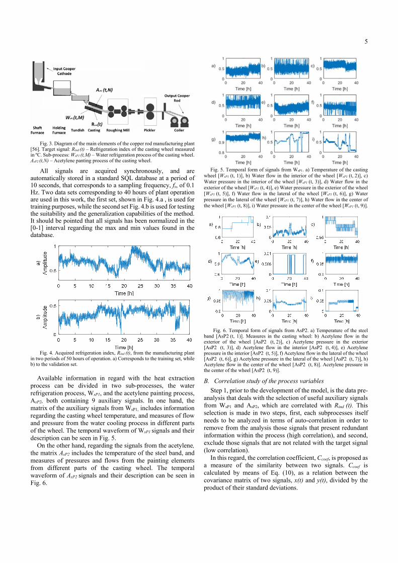
 Fig. 3. Diagram of the main elements of the copper rod manufacturing plant

[56]. Target signal: Rind (t) – Refrigeration index of the casting wheel measured in ºC. Sub-process: WsP1 (t,M) – Water refrigeration process of the casting wheel. AsP2 (t,N) – Acetylene panting process of the casting wheel.

All signals are acquired synchronously, and are automatically stored in a standard SQL database at a period of 10 seconds, that corresponds to a sampling frequency, fs, of 0.1 Hz. Two data sets corresponding to 40 hours of plant operation are used in this work, the first set, shown in Fig. 4.a , is used for training purposes, while the second set Fig. 4.b is used for testing the suitability and the generalization capabilities of the method. It should be pointed that all signals has been normalized in the [0-1] interval regarding the max and min values found in the database.

Fig. 4. Acquired refrigeration index, Rind (t), from the manufacturing plant in two periods of 50 hours of operation. a) Corresponds to the training set, while b) to the validation set.

Available information in regard with the heat extraction

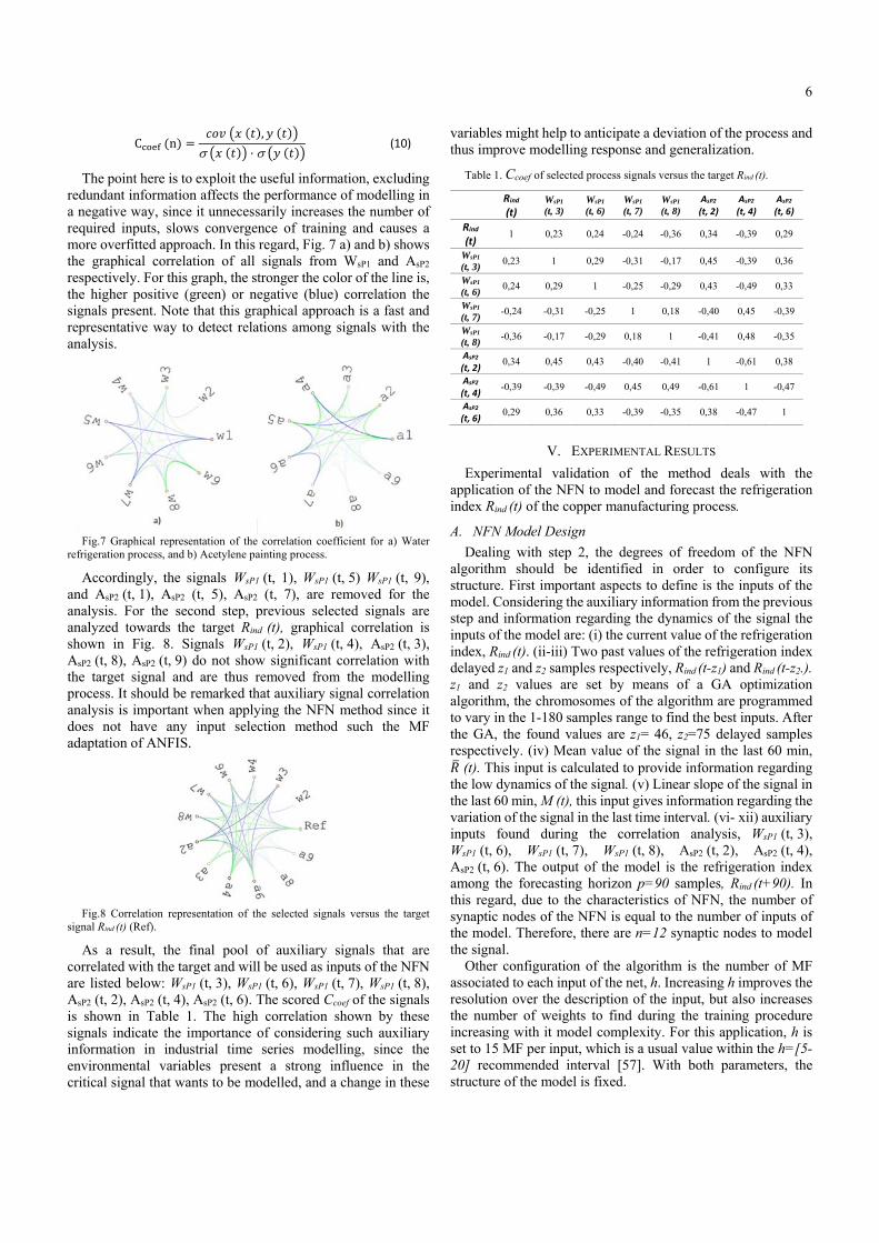
process can be divided in two sub-processes, the water refrigeration process, WsP1, and the acetylene painting process, AsP2, both containing 9 auxiliary signals. In one hand, the matrix of the auxiliary signals from WsP1, includes information regarding the casting wheel temperature, and measures of flow and pressure from the water cooling process in different parts of the wheel. The temporal waveform of WsP1 signals and their description can be seen in Fig. 5.

On the other hand, regarding the signals from the acetylene, the matrix AsP2 includes the temperature of the steel band, and measures of pressures and flows from the painting elements from different parts of the casting wheel. The temporal waveform of AsP2 signals and their description can be seen in Fig. 6.

 

Fig. 5. Temporal form of signals from WsP1. a) Temperature of the casting wheel [WsP1 (t, 1)], b) Water flow in the interior of the wheel [WsP1 (t, 2)], c) Water pressure in the interior of the wheel [WsP1 (t, 3)], d) Water flow in the exterior of the wheel [WsP1 (t, 4)], e) Water pressure in the exterior of the wheel [WsP1 (t, 5)], f) Water flow in the lateral of the wheel [WsP1 (t, 6)], g) Water pressure in the lateral of the wheel [WsP1 (t, 7)], h) Water flow in the center of the wheel [WsP1 (t, 8)], i) Water pressure in the center of the wheel [WsP1 (t, 9)].

Fig. 6. Temporal form of signals from AsP2. a) Temperature of the steel band [AsP2 (t, 1)]. Measures in the casting wheel: b) Acetylene flow in the exterior of the wheel [AsP2 (t, 2)], c) Acetylene pressure in the exterior [AsP2 (t, 3)], d) Acetylene flow in the interior [AsP2 (t, 4)], e) Acetylene pressure in the interior [AsP2 (t, 5)], f) Acetylene flow in the lateral of the wheel [AsP2 (t, 6)], g) Acetylene pressure in the lateral of the wheel [AsP2 (t, 7)], h) Acetylene flow in the center of the wheel [AsP2 (t, 8)]. Acetylene pressure in the center of the wheel [AsP2 (t, 9)].

B. Correlation study of the process variables

Step 1, prior to the development of the model, is the data pre-analysis that deals with the selection of useful auxiliary signals from WsP1 and AsP2, which are correlated with Rind (t). This selection is made in two steps, first, each subprocesses itself needs to be analyzed in terms of auto-correlation in order to remove from the analysis those signals that present redundant information within the process (high correlation), and second, exclude those signals that are not related with the target signal (low correlation).

In this regard, the correlation coefficient, Ccoef, is proposed as a measure of the similarity between two signals. Ccoef is calculated by means of Eq. (10), as a relation between the covariance matrix of two signals, x(t) and y(t), divided by the product of their standard deviations.

6

C n ,

  (10) 

The point here is to exploit the useful information, excluding redundant information affects the performance of modelling in a negative way, since it unnecessarily increases the number of required inputs, slows convergence of training and causes a more overfitted approach. In this regard, Fig. 7 a) and b) shows the graphical correlation of all signals from WsP1 and AsP2

respectively. For this graph, the stronger the color of the line is, the higher positive (green) or negative (blue) correlation the signals present. Note that this graphical approach is a fast and representative way to detect relations among signals with the analysis.

   Fig.7 Graphical representation of the correlation coefficient for a) Water

refrigeration process, and b) Acetylene painting process.

Accordingly, the signals WsP1 (t, 1), WsP1 (t, 5) WsP1 (t, 9), and AsP2 (t, 1), AsP2 (t, 5), AsP2 (t, 7), are removed for the analysis. For the second step, previous selected signals are analyzed towards the target Rind (t), graphical correlation is shown in Fig. 8. Signals WsP1 (t, 2), WsP1 (t, 4), AsP2 (t, 3), AsP2 (t, 8), AsP2 (t, 9) do not show significant correlation with the target signal and are thus removed from the modelling process. It should be remarked that auxiliary signal correlation analysis is important when applying the NFN method since it does not have any input selection method such the MF adaptation of ANFIS.

 Fig.8 Correlation representation of the selected signals versus the target

signal Rind (t) (Ref).

As a result, the final pool of auxiliary signals that are correlated with the target and will be used as inputs of the NFN are listed below: WsP1 (t, 3), WsP1 (t, 6), WsP1 (t, 7), WsP1 (t, 8), AsP2 (t, 2), AsP2 (t, 4), AsP2 (t, 6). The scored Ccoef of the signals is shown in Table 1. The high correlation shown by these signals indicate the importance of considering such auxiliary information in industrial time series modelling, since the environmental variables present a strong influence in the critical signal that wants to be modelled, and a change in these

variables might help to anticipate a deviation of the process and thus improve modelling response and generalization.

Table 1. Ccoef of selected process signals versus the target Rind (t).

Rind 

(t) WsP1 (t, 3)

WsP1 (t, 6)

WsP1 (t, 7)

WsP1 (t, 8)

AsP2 (t, 2)

AsP2 (t, 4)

AsP2 (t, 6)

Rind 

(t) 1 0,23 0,24 -0,24 -0,36 0,34 -0,39 0,29

WsP1 (t, 3)

0,23 1 0,29 -0,31 -0,17 0,45 -0,39 0,36

WsP1 (t, 6)

0,24 0,29 1 -0,25 -0,29 0,43 -0,49 0,33

WsP1 (t, 7)

-0,24 -0,31 -0,25 1 0,18 -0,40 0,45 -0,39

WsP1 (t, 8)

-0,36 -0,17 -0,29 0,18 1 -0,41 0,48 -0,35

AsP2 (t, 2)

0,34 0,45 0,43 -0,40 -0,41 1 -0,61 0,38

AsP2 (t, 4)

-0,39 -0,39 -0,49 0,45 0,49 -0,61 1 -0,47

AsP2 (t, 6)

0,29 0,36 0,33 -0,39 -0,35 0,38 -0,47 1

V. EXPERIMENTAL RESULTS

Experimental validation of the method deals with the application of the NFN to model and forecast the refrigeration index Rind (t) of the copper manufacturing process.

A. NFN Model Design

Dealing with step 2, the degrees of freedom of the NFN algorithm should be identified in order to configure its structure. First important aspects to define is the inputs of the model. Considering the auxiliary information from the previous step and information regarding the dynamics of the signal the inputs of the model are: (i) the current value of the refrigeration index, Rind (t). (ii-iii) Two past values of the refrigeration index delayed z1 and z2 samples respectively, Rind (t-z1) and Rind (t-z2.). z1 and z2 values are set by means of a GA optimization algorithm, the chromosomes of the algorithm are programmed to vary in the 1-180 samples range to find the best inputs. After the GA, the found values are z1= 46, z2=75 delayed samples respectively. (iv) Mean value of the signal in the last 60 min,

(t). This input is calculated to provide information regarding the low dynamics of the signal. (v) Linear slope of the signal in the last 60 min, M (t), this input gives information regarding the variation of the signal in the last time interval. (vi- xii) auxiliary inputs found during the correlation analysis, WsP1 (t, 3), WsP1 (t, 6), WsP1 (t, 7), WsP1 (t, 8), AsP2 (t, 2), AsP2 (t, 4), AsP2 (t, 6). The output of the model is the refrigeration index among the forecasting horizon p=90 samples, Rind (t+90). In this regard, due to the characteristics of NFN, the number of synaptic nodes of the NFN is equal to the number of inputs of the model. Therefore, there are n=12 synaptic nodes to model the signal.

Other configuration of the algorithm is the number of MF associated to each input of the net, h. Increasing h improves the resolution over the description of the input, but also increases the number of weights to find during the training procedure increasing with it model complexity. For this application, h is set to 15 MF per input, which is a usual value within the h=[5-20] recommended interval [57]. With both parameters, the structure of the model is fixed.

7

B. NFN model Training and Validation

In order to face step 3, the parameters of the training algorithm must be set. In this regard, as the NFN is trained by means of the backpropagation method, the NFN learning rate, α, that adjust the learning convergence of the algorithm must be set. It should be noticed that depending on the complexity of the problem, high values of α might lead to an unstable solution. For this reason, a lower learning rate between 0.001< α<0.05 is recommended [58]. For this application, α = 0.003.

The last parameter is the number of training iterations. The weights will be adapted by introducing the input data a defined number of iterations, as the number of iteration increases, the same data is passed through the model that results in a more overfitting approach and a loss of generalization in the output. In this sense, the number of training iterations is set to 10.

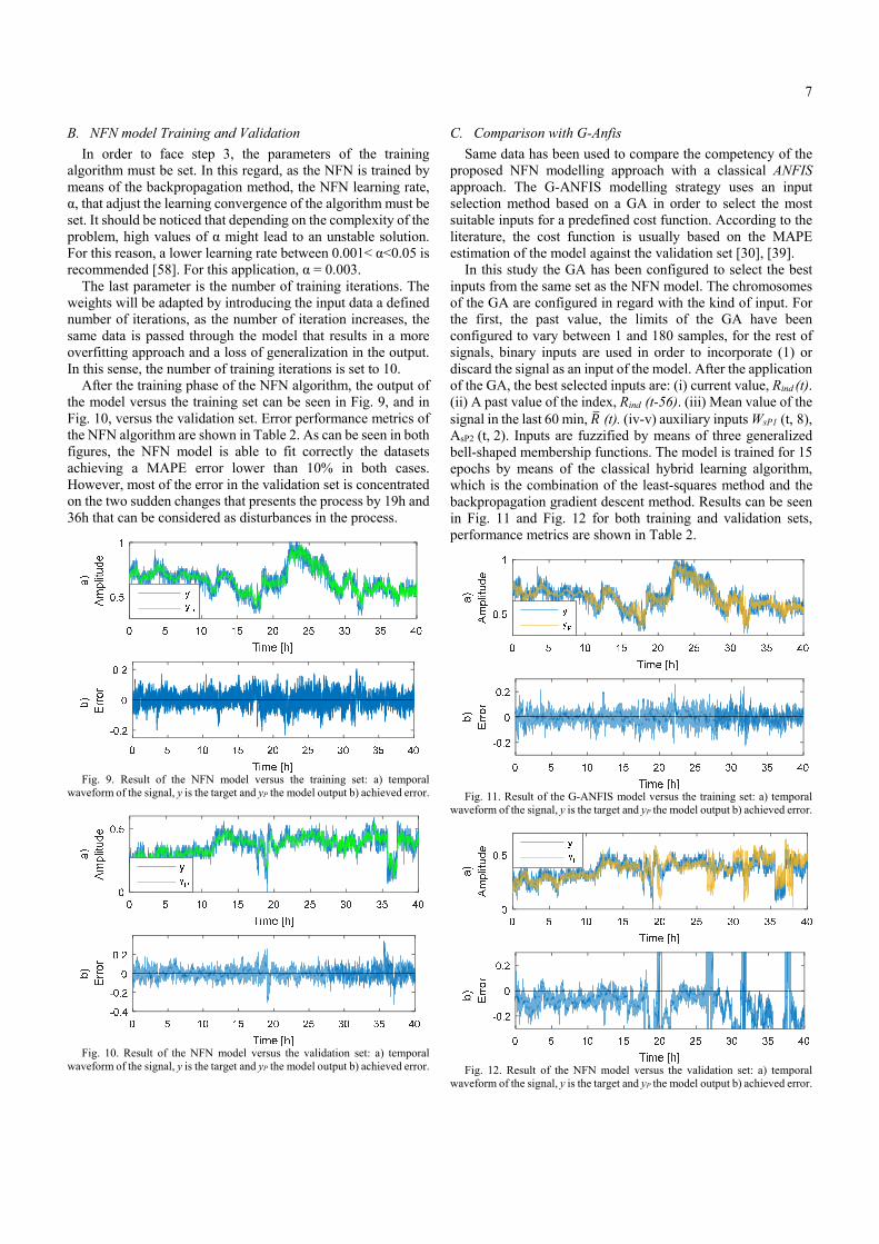
After the training phase of the NFN algorithm, the output of the model versus the training set can be seen in Fig. 9, and in Fig. 10, versus the validation set. Error performance metrics of the NFN algorithm are shown in Table 2. As can be seen in both figures, the NFN model is able to fit correctly the datasets achieving a MAPE error lower than 10% in both cases. However, most of the error in the validation set is concentrated on the two sudden changes that presents the process by 19h and 36h that can be considered as disturbances in the process.

Fig. 9. Result of the NFN model versus the training set: a) temporal waveform of the signal, y is the target and yP the model output b) achieved error.

Fig. 10. Result of the NFN model versus the validation set: a) temporal waveform of the signal, y is the target and yP the model output b) achieved error.

C. Comparison with G-Anfis

Same data has been used to compare the competency of the proposed NFN modelling approach with a classical ANFIS approach. The G-ANFIS modelling strategy uses an input selection method based on a GA in order to select the most suitable inputs for a predefined cost function. According to the literature, the cost function is usually based on the MAPE estimation of the model against the validation set [30], [39].

In this study the GA has been configured to select the best inputs from the same set as the NFN model. The chromosomes of the GA are configured in regard with the kind of input. For the first, the past value, the limits of the GA have been configured to vary between 1 and 180 samples, for the rest of signals, binary inputs are used in order to incorporate (1) or discard the signal as an input of the model. After the application of the GA, the best selected inputs are: (i) current value, Rind (t). (ii) A past value of the index, Rind (t-56). (iii) Mean value of the signal in the last 60 min, (t). (iv-v) auxiliary inputs WsP1 (t, 8), AsP2 (t, 2). Inputs are fuzzified by means of three generalized bell-shaped membership functions. The model is trained for 15 epochs by means of the classical hybrid learning algorithm, which is the combination of the least-squares method and the backpropagation gradient descent method. Results can be seen in Fig. 11 and Fig. 12 for both training and validation sets, performance metrics are shown in Table 2.

Fig. 11. Result of the G-ANFIS model versus the training set: a) temporal waveform of the signal, y is the target and yP the model output b) achieved error.

Fig. 12. Result of the NFN model versus the validation set: a) temporal waveform of the signal, y is the target and yP the model output b) achieved error.

8

Table 2. Performance metrics of both NFN and GANFIS algorithms

NFN G- ANFIS

Merit Factor Trn. Val. Trn. Val.

RMSE 0.047 0.063 0.053 0.095

MAE 0.191 0.228 0.204 0.316

MAPE (%) 5.53 9.51 6.58 16.14

As can be seen in both training and validation responses, the NFN presents a smoother response which is concentrated in following the mean signal value without incurring in the generation of outliers. This fact is reflexed in the low achieved RMSE value of the algorithm, which is more sensitive to samples displaced from the mean value. Furthermore, the error in the training set presents a Gaussian distribution for both NFN and GANFIS modelling methods, which indicates the goodness of both methods (MAPE<7% in training). In this regard, the G-ANFIS method also achieves a good response in the training set, but it presents a more overfitting response in the validation set. This fact can be appreciated in Fig. 12 b) as an increase of the error when a sudden change in the process is appreciated (around 19 and 36h of plant operation). This error increase is due to the over-adjustment of the ANFIS model to the signals. This results indicate and the suitability to apply NFN to the modelling of industrial time series. However, further modifications in the NFN algorithm can be made in order to enhance the results when dealing with industrial time series, such modifications include the particularization of the MF to the data density ranges of the signal, or the dynamic learning rate adaptation.

VI. CONCLUSIONS

This paper presents the Neo-Fuzzy Neuron (NFN) for modelling industrial time series. The proposed approach takes advantage of the process correlations in order to select the most suitable set of inputs to enhance performance of a NFN method.

The proposed method has been successfully applied to forecast the evolution of the refrigeration index from a copper manufacturing plant in terms of low error and high generalization capabilities for a prediction horizon of 15 minutes. The results indicate that the method is suitable to be applied in industrial processes which fastest dynamics is measured in seconds, which is an affordable range of industrial applications. Note that is the first time that NFN has been applied to the modelling of industrial processes.

Furthermore, a comparative with the classical ANFIS method has been made. The results show that the NFN method adapts better to the available training dataset increasing generalization capabilities towards the validation set while reducing modelling complexity.

Future work is concentrated on the modification of the NFN method to improve modelling accuracy while optimizing the structure of the network. In this regard, the main concerns are the adaptation of the MF to the data distribution of each input, rather than the classical equidistant MF. Also, other point is the adaptive modification of the learning rate of the algorithm in regard with the achieved error to improve the training procedure.

VII. REFERENCES [1] S. Wang, D. Li, and C. Zhang, “Towards smart factory for industry

4.0: a self-organized multi-agent system with big data based feedback and coordination,” Comput. Networks, vol. 101, pp. 158–168, 2016.

[2] M. Delgado Prieto, D. Zurita Millan, W. Wang, A. Machado Ortiz, J. A. Ortega Redondo, and L. Romeral Martinez, “Self-Powered Wireless Sensor Applied to Gear Diagnosis Based on Acoustic Emission,” IEEE Trans. Instrum. Meas., vol. 65, no. 1, pp. 15–24, Jan. 2016.

[3] C.-H. (Robert) Hsu, “Industrial technologies and applications for the Internet of Things,” Computer Networks, vol. 101. pp. 1–4, 2016.

[4] D. Kwon, M. R. Hodkiewicz, J. Fan, T. Shibutani, and M. G. Pecht, “IoT-Based Prognostics and Systems Health Management for Industrial Applications,” IEEE Access, vol. 4, pp. 3659–3670, 2016.

[5] J. Lee, B. Bagheri, and H.-A. Kao, “A Cyber-Physical Systems architecture for Industry 4.0-based manufacturing systems,” 2015.

[6] X.-W. Xue-Wen Chen and X. Xiaotong Lin, “Big Data Deep Learning: Challenges and Perspectives,” IEEE Access, vol. 2, pp. 514–525, 2014.

[7] T. Niesen, C. Houy, P. Fettke, and P. Loos, “Towards an Integrative Big Data Analysis Framework for Data-Driven Risk Management in Industry 4.0,” in 2016 49th Hawaii International Conference on System Sciences (HICSS), 2016, pp. 5065–5074.

[8] M. Xia, T. Li, Y. Zhang, and C. W. de Silva, “Closed-loop design evolution of engineering system using condition monitoring through internet of things and cloud computing,” Comput. Networks, vol. 101, pp. 5–18, 2016.

[9] D. Gorecky, M. Schmitt, M. Loskyll, and D. Zuhlke, “Human-machine-interaction in the industry 4.0 era,” in 2014 12th IEEE International Conference on Industrial Informatics (INDIN), 2014, pp. 289–294.

[10] J. Nelles, S. Kuz, A. Mertens, and C. M. Schlick, “Human-centered design of assistance systems for production planning and control: The role of the human in Industry 4.0,” in 2016 IEEE International Conference on Industrial Technology (ICIT), 2016, pp. 2099–2104.

[11] T. Stock and G. Seliger, “Opportunities of Sustainable Manufacturing in Industry 4.0,” Procedia CIRP, vol. 40, pp. 536–541, 2016.

[12] C. Faller and D. Feldmüller, “Industry 4.0 Learning Factory for regional SMEs,” Procedia CIRP, vol. 32, pp. 88–91, 2015.

[13] K.-S. Wang, “Towards zero-defect manufacturing (ZDM)—a data mining approach,” Adv. Manuf., vol. 1, no. 1, pp. 62–74, 2013.

[14] F. T. Cheng, H. Tieng, H. C. Yang, M. H. Hung, Y. C. Lin, C. F. Wei, and Z. Y. Shieh, “Industry 4.1 for Wheel Machining Automation,” IEEE Robotics and Automation Letters, vol. 1, no. 1. pp. 332–339, 2016.

[15] W. Y. Wang K, “Data mining for zero–defect manufacturing,” Tpir Acad. Press London, 2012.

[16] A. K. S. Jardine, D. Lin, and D. Banjevic, “A review on machinery diagnostics and prognostics implementing condition-based maintenance,” Mech. Syst. Signal Process., vol. 20, no. 7, pp. 1483–1510, 2006.

[17] J. Z. Sikorska, M. Hodkiewicz, and L. Ma, “Prognostic modelling options for remaining useful life estimation by industry,” Mech. Syst. Signal Process., vol. 25, no. 5, pp. 1803–1836, 2011.

[18] S. Yin, S. X. Ding, X. Xie, and H. Luo, “A Review on Basic Data-Driven Approaches for Industrial Process Monitoring,” IEEE Trans. Ind. Electron., vol. 61, no. 11, pp. 6418–6428, Nov. 2014.

[19] H. Hanli Wei, Y. Yongmao Xu, and R. Re Zhang, “Neural networks based model predictive control of an industrial polypropylene process,” in Proceedings of the International Conference on Control Applications, 2002, vol. 1, pp. 397–402.

[20] M. V. V. N. Sriram, N. K. Singh, and G. Rajaraman, “Neuro fuzzy modelling of Basic Oxygen Furnace and its comparison with Neural Network and GRNN models,” in 2010 IEEE International Conference on Computational Intelligence and Computing Research, 2010, pp. 1–8.

[21] C. Chen, B. Zhang, G. Vachtsevanos, M. Orchard, C. Chaochao, Z. Bin, G. Vachtsevanos, and M. Orchard, “Machine condition prediction based on adaptive neuro–fuzzy and high-order particle filtering,” Ind. Electron. IEEE Trans., vol. 58, no. 9, pp. 4353–4364, 2011.

[22] V. Kolodyazhniy, Y. Bodyanskiy, and P. Otto, “Universal Approximator Employing Neo-Fuzzy Neurons,” in Computational Intelligence, Theory and Applications, Berlin, Heidelberg: Springer

9

Berlin Heidelberg, 2005, pp. 631–640. [23] Y. Bodyanskiy, Y. Bodyanskiy, I. Kokshenev, V. Kolodyazhniy, and

V. K. Ye. Bodyanskiy, I. Kokshenev, An Adaptive Learning Algorithm for a Neo Fuzzy Neuron. 2003, pp. 375–379.

[24] Y. V. Bodyanskiy, O. K. Tyshchenko, and D. S. Kopaliani, “A Multidimensional Cascade Neuro-Fuzzy System with Neuron Pool Optimization in Each Cascade,” Int. J. Inf. Technol. Comput. Sci., vol. 6, no. 8, p. 11, 2014.

[25] J. Lee, J. Ni, D. Djurdjanovic, H. Qiu, and H. Liao, “Intelligent prognostics tools and e-maintenance,” Comput. Ind., vol. 57, no. 6, pp. 476–489, 2006.

[26] O. Myklebust, “Zero Defect Manufacturing: A Product and Plant Oriented Lifecycle Approach,” Procedia CIRP, vol. 12, no. 0, pp. 246–251, 2013.

[27] J. Lee, E. Lapira, B. Bagheri, and H. Kao, “Recent advances and trends in predictive manufacturing systems in big data environment,” Manuf. Lett., vol. 1, no. 1, pp. 38–41, 2013.

[28] L. Baldacci, M. Golfarelli, D. Lombardi, and F. Sami, “Natural gas consumption forecasting for anomaly detection,” Expert Syst. Appl., vol. 62, pp. 190–201, 2016.

[29] D. Zurita-Millan, M. Delgado-Prieto, J. J. Saucedo-Dorantes, J. A. Cariño-Corrales, R. A. Osornio-Rios, J. A. Ortega Redondo, and R. de J. Romero-Troncoso, “Vibration signal forecasting on rotating machinery by means of signal decomposition and neuro-fuzzy modeling,” Shock Vib., 2016.

[30] Z. Hu, Y. Bao, T. Xiong, and R. Chiong, “Hybrid filter–wrapper feature selection for short-term load forecasting,” Eng. Appl. Artif. Intell., vol. 40, pp. 17–27, Apr. 2015.

[31] F. Keynia, “A new feature selection algorithm and composite neural network for electricity price forecasting,” Eng. Appl. Artif. Intell., vol. 25, no. 8, pp. 1687–1697, 2012.

[32] K. Kampouropoulos, F. Andrade, A. Garcia, and L. Romeral, “A Combined Methodology of Adaptive Neuro-Fuzzy Inference System and Genetic Algorithm for Short-term Energy Forecasting,” Adv. Electr. Comput. Eng., vol. 14, no. 1, pp. 9–14, 2014.

[33] A. D. Back and T. P. Trappenberg, “Selecting inputs for modeling using normalized higher order statistics and independent component analysis,” IEEE Trans. Neural Networks, vol. 12, no. 3, pp. 612–617, May 2001.

[34] X. Deng, X. Zeng, P. Vroman, and L. Koehl, “Selection of relevant variables for industrial process modeling by combining experimental data sensitivity and human knowledge,” Eng. Appl. Artif. Intell., vol. 23, no. 8, pp. 1368–1379, 2010.

[35] F. M. Bianchi, E. De Santis, A. Rizzi, and A. Sadeghian, “Short-Term Electric Load Forecasting Using Echo State Networks and PCA Decomposition,” IEEE Access, vol. 3, pp. 1931–1943, 2015.

[36] C. Brighenti and M. Á. Sanz-Bobi, “Auto-regressive processes explained by self-organized maps. Application to the detection of abnormal behavior in industrial processes.,” IEEE Trans. Neural Netw., vol. 22, no. 12, pp. 2078–90, Dec. 2011.

[37] C. W. Frey, “Monitoring of complex industrial processes based on self-organizing maps and watershed transformations,” in Industrial Technology (ICIT), 2012 IEEE International Conference on, 2012, pp. 1041–1046.

[38] M. Domínguez, J. J. Fuertes, I. Díaz, M. A. Prada, S. Alonso, and A. Morán, “Monitoring industrial processes with SOM-based dissimilarity maps,” Expert Syst. Appl., vol. 39, no. 8, pp. 7110–7120, 2012.

[39] K. Kampouropoulos, J. J. Cardenas, F. Giacometto, and L. Romeral, “An energy prediction method using Adaptive Neuro-Fuzzy Inference System and Genetic Algorithms,” in Industrial Electronics (ISIE), 2013 IEEE International Symposium on, 2013, pp. 1–6.

[40] Y. Ren, P. N. Suganthan, and N. Srikanth, “A Comparative Study of Empirical Mode Decomposition-Based Short-Term Wind Speed Forecasting Methods,” IEEE Trans. Sustain. Energy, vol. 6, no. 1, pp. 236–244, Jan. 2015.

[41] Z. Guo, W. Zhao, H. Lu, and J. Wang, “Multi-step forecasting for wind speed using a modified EMD-based artificial neural network model,” Renew. Energy, vol. 37, no. 1, pp. 241–249, Jan. 2012.

[42] W. Wang, K. Chau, L. Qiu, and Y. Chen, “Improving forecasting accuracy of medium and long-term runoff using artificial neural network based on EEMD decomposition.,” Environ. Res., vol. 139, pp. 46–54, May 2015.

[43] J. Eynard, S. Grieu, and M. Polit, “Wavelet-based multi-resolution analysis and artificial neural networks for forecasting temperature

and thermal power consumption,” Eng. Appl. Artif. Intell., vol. 24, no. 3, pp. 501–516, Apr. 2011.

[44] A. Zamaniyan, F. Joda, A. Behroozsarand, and H. Ebrahimi, “Application of artificial neural networks (ANN) for modeling of industrial hydrogen plant,” Int. J. Hydrogen Energy, vol. 38, no. 15, pp. 6289–6297, 2013.

[45] E. Ceperic, V. Ceperic, and A. Baric, “A Strategy for Short-Term Load Forecasting by Support Vector Regression Machines,” IEEE Trans. Power Syst., vol. 28, no. 4, pp. 4356–4364, Nov. 2013.

[46] L. Dezhi, W. Wang, and F. Ismail, “Fuzzy Neural Network Technique for System State Forecasting,” Cybern. IEEE Trans., vol. 43, no. 5, pp. 1484–1494, 2013.

[47] B. Dehkordi, M. Moallem, and A. Parsapour, “Predicting Foaming Slag Quality in Electric Arc Furnace Using Power Quality Indices and Fuzzy Method,” IEEE Trans. Instrum. Meas., vol. 60, no. 12, pp. 3845–3852, Dec. 2011.

[48] K. T. Chaturvedi, M. Pandit, and L. Srivastava, “Modified neo-fuzzy neuron-based approach for economic and environmental optimal power dispatch,” Appl. Soft Comput., vol. 8, no. 4, pp. 1428–1438, 2008.

[49] Y. Bodyanskiy, I. Pliss, and O. Vynokurova, “Flexible Neo-fuzzy Neuron and Neuro-fuzzy Network for Monitoring Time Series Properties,” Inf. Technol. Manag. Sci., vol. 16, no. 1, pp. 47–52, Jan. 2013.

[50] A. Soualhi, G. Clerc, H. Razik, and F. Rivas, “Long-term prediction of bearing condition by the neo-fuzzy neuron,” in 2013 9th IEEE International Symposium on Diagnostics for Electric Machines, Power Electronics and Drives (SDEMPED), 2013, pp. 586–591.

[51] T. Yamakawa, E. Uchino, T. Miki, and H. Kusanagi, “A neo fuzzy neuron and its applications to system identification and prediction of the system behavior,” in Proc. 2nd Int. Conf. on Fuzzy Logic and Neural Networks, 1992, pp. 477–483.

[52] E. Uchino and T. Yamakawa, “Soft Computing Based Signal Prediction, Restoration, and Filtering,” in Intelligent Hybrid Systems, Boston, MA: Springer US, 1997, pp. 331–351.

[53] T. Miki and T. Yamakawa, “Analog Implementation of Neo-Fuzzy Neuron and Its On-board Learning.”

[54] E. Uchino and T. Yamakawa, “System Modeling by a Neo-Fuzzy-Neuron with Applications to Acoustic and Chaotic Systems,” Int. J. Artif. Intell. Tools, vol. 04, no. 01n02, pp. 73–91, Jun. 1995.

[55] A. Davydenko and R. Fildes, “Measuring forecasting accuracy: The case of judgmental adjustments to SKU-level demand forecasts,” Int. J. Forecast., vol. 29, no. 3, pp. 510–522, Jul. 2013.

[56] O. Rentz, “Report on BAT in German Copper Production (Final Draft).,” University Karlsruhe (DFIU)., 1999.

[57] A. M. Silva, W. Caminhas, A. Lemos, and F. Gomide, “A fast learning algorithm for evolving neo-fuzzy neuron,” Appl. Soft Comput., vol. 14, pp. 194–209, 2014.

[58] Y. V. Bodyanskiy, O. K. Tyshchenko, and D. S. Kopaliani, “An Extended Neo-Fuzzy Neuron and its Adaptive Learning Algorithm,” Int. J. Intell. Syst. Appl., vol. 7, no. 2, p. 21, 2015.

BIOGRAPHIES Daniel Zurita received his M.S. degree in electronics engineering from the

UPC in 2013. He is currently a Ph.D. student in the Electronic degree of the UPC. His research interests include fault diagnosis and prognosis in electric machines, industrial process monitoring, fault detection algorithms, machine learning and signal processing methods.

Miguel Delgado received the M.S. and Ph.D. degrees in Electronics Engineering and the Ph.D. degree from the UPC, Barcelona, Spain in 2007 and 2012 respectively. From 2004 to 2008 he was a Teaching Assistant in the Electronic Engineering Department of the UPC. In 2008 he joined the MCIA Center, where he is currently a research assistant. His research interests include fault detection algorithms, machine learning, signal processing methods and embedded systems.

Jesus A. Carino received the M.S. degree in electrical engineering from the University of Guanajuato, Guanajuato, México, in 2012. Currently, he is working toward the Ph.D. degree under CONACyT scholarship program at the MCIA Center in UPC, Terrassa, Spain. His research interests include digital signal processing on FPGAs for applications in mechatronics, fault diagnosis in electric machines, fault detection algorithms and pattern recognition.

10

Juan A. Ortega received the M.S. Telecommunication Engineer and Ph.D. degrees in Electronics from the Technical University of Catalonia (UPC) in 1994 and 1997, respectively. In 1994, he joined the UPC Department of Electronic Engineering. Since 2001 he belongs to the Motion Control and Industrial Applications research group. His research activities include: motor diagnosis, signal acquisition, smart sensors, embedded systems and remote labs.

Guy Clerc (M’90–SM’10) was born in Libourne, France, on November 30, 1960. He received the Electrical Engineering degree and the Ph.D. degree in electrical engineering from the Ecole Centrale de Lyon, Écully, France, in 1984 and 1989, respectively. He is a Professor of electrical engineering at the Université Claude Bernard Lyon 1, Villeurbanne, France. He conducts research on control and diagnosis of induction machines with the Laboratoire Ampère–UMR 5005, Villeurbanne, France.