Industrial Policy and Competition

P. Aghion, M. Dewatripont, L. Du, A. Harrison & P. Legros

June 28, 2011

1 Introduction

In the aftermath of WWII, several developing countries opted for policies aimedat promoting new infant industries or at protecting local traditional activitiesfrom competition by products from more advanced countries. Thus severalLatin American countries advocated import substitution policies, whereby localindustries would more fully benefit from domestic demand. East Asian countrieslike Korea or Japan, rather than advocating import substitution policies, wouldfavor export promotion, which in turn would be achieved partly through tariffsand non-tariff barriers and partly through maintaining undervalued exchangerates. For at least two or three decades after WWII, these policies, whichbelong to what is commonly referred to as “industrial policy,” remained fairlynoncontroversial as both groups of countries were growing at fast rates.

However, the economic slowdown in the 70s in Latin America and Japan inthe late 90s, generated a growing skepticism about the role of industrial policyin the process of economic development. On the empirical front, the debate waslaunched by Krueger and Tuncer (1982) who analyzed the effects of industrialpolicy in Turkey in the 60s, and “show” that firms or industries not protectedby tariff measures were characterized by higher productivity in growth ratesthan protected industries.1 On the theoretical front, the provision by domesticgovernments of subsidies or trade protection targeted to particular firms orindustries, has come under disrepute among academics mainly on the groundthat it prevents competition and allows governments to pick winners (and, morerarely, to name losers) in a discretionary fashion, thereby increasing the scope forcapture of governments by vested interests. This argument appears to have wonover traditional counteracting considerations, in particular those based upon theinfant industry idea (e.g.,see Greenwald and Stiglitz (2006)).2 This disreputehas affected not only the selection and promotion of national champions – what

1However, see Harrison (1994).2For an overview of infant-industry models and empirical evidence, see Harrison and

Rodriguez-Clare (2010). The infant-industry argument could be summarized as follows.Consider a local economy that includes both a traditional sector (especially agriculture) andan industry in its infancy. Production costs in industry are initially high, but “learning bydoing” decrease these costs over time, even faster as the volume of activity in this area is high.In addition, increased productivity which is a consequence of this learning by doing phase haspositive spillovers on the rest of the economy, ie it increases the potential rate of growth also

1

could be termed industrial policy in the narrow sense - but also any kind ofpublic intervention going beyond horizontal supply-side policies with the aimto influence sectoral developments and the composition of aggregate output. afirst argument against industrial policy and the infant industry argument, is thatgovernments are not particularly good at picking winners, and providing themwith an excuse to subsidize particular firms or sectors might end up favouringthe emergence of industrial lobbies.

Yet, new considerations have emerged over the recent period, which inviteus to revisit the issue. First, climate change and the increasing awareness of thefact that without government intervention aimed at encouraging clean produc-tion and clean innovation, global warming will intensify and generate negativeexternalities (droughts, deforestations, migrations, conflicts) worldwide. Be-yond the pricing of this externality through cap-and-trade systems or carbontaxation, many governments have engaged in targeted intervention to encour-age the development of alternative technologies in the production (e.g.,fromrenewables) or the use (e.g. by efficient housing) of energy. Second, the re-cent financial crisis has prompted several governments, including the US, toprovide support to particular industries (e.g., the automobile or green sectors).Also, an increasing number of scholars (in particular in the US) are denouncingthe danger of laissez-faire policies that lead developed countries to specializein upstream R&D and in services while outsourcing all manufacturing tasks todeveloping countries where unskilled labor costs are lower. They point to thefact that countries like Germany or Japan have better managed to maintainintermediate manufacturing segments through pursuing more active industrialpolicies, and that this in turn has allowed them to benefit more from outsourcingthe other, less human capital-intensive segments.

In this paper we argue that the debate on industrial policy should no longerbe “existential”, i.e.,about whether sectoral policies should be precluded alto-gether or not, but rather on how such policies should be designed and governedso as to foster growth and welfare. Our focus is on the relationship betweensectoral policy and product market competition. In the first part of the paperwe develop a theoretical framework in which two firms may choose either to op-erate in the same “higher-growth” sector (we refer to this as the choice to focuson the same technology) or they may choose to operate in different sectors, in-cluding in “lower-growth” sectors in order to reduce the intensity of competitionamong them (we refer to this as the choice to diversify). When firms focus onthe same high-growth sector they generate more innovation and growth for tworeasons: first, because the size of innovations, and therefore the post-innovationrents, are higher in a higher-growth sector; second, because when the two firmschoose to operate in the same sector they compete more intensely, which in turn

in the traditional sector. In this case, a total and instantaneous liberalization of internationaltrade can be detrimental to the growth of the local economy, as it might inhibit the activityof the local industry whose production costs are initially high: what will happen in this caseis that the local demand for industrial products will turn to foreign importers. It means thatlearning by doing in the local industry will be slowed itself, which will reduce the externalitiesof growth from this sector towards the traditional sector.

2

induces both firms to invest more in innovation in order to escape competitionwith the rival firm (see Aghion et al (2005)). The more intense competitionwithin a sector, the more firms innovate if they operate in the same sector.At the same time, more intense competition within sectors may induce firmsto choose diversity as an alternative way to avoid competition. This is whereindustrial policy comes into play: by inducing the two firms to operate in thesame sector, the government induces firms to innovate “vertically” rather thandifferentiate “horizontally” in order to escape competition with the other firm.The more intense within-sector competition, the more growth-enhancing it is toinduce both firms to operate in the same “high-growth” sector. In other words,there is a complementarity between product market competition and sectoralpolicy in fostering innovation and growth.

In the second part of the paper we test for the complementarity betweencompetition and industrial policy. We use a panel of medium and large Chineseenterprises for the period 1998 through 2007. Our measures of industrial policyare: (1) subsidies, allocated at the firm level, and (2) trade tariffs, which aredetermined at the sector level. We measure competition in two ways: usingindustry-level Lerner indices, which capture the degree of markups over cost,and the extent to which industrial policies preserve or increase competition.We then look at the effect on productivity, productivity growth, and productinnovation, of policies that preserve or increase competition through the sectoraldispersion of subsidies.

Our results suggest that if subsidies are allocated to competitive sectors (asmeasured by the Lerner index) and allocated in such a way as to preserve orincrease competition, then the net impacts of subsidies on productivity, produc-tivity growth, and product innovation measured by the share of new products intotal sales, become positive and significant. In other words, targeting can havebeneficial effects depending on both the degree of competition in the targetedsector as well as depending on how the targeting is done.

Most closely related to our analysis in this paper is Nunn and Trefler (2010).Using cross-country industry-level panel data, they analyze whether, as sug-gested by the argument of “infant industry”, the growth of productivity in acountry is positively affected by the measure in which tariff protection is biasedin favor of activities and sectors that are “skill-intensive”, that is to say, usemore intensely skilled workers. They find a significant positive correlation be-tween productivity growth and the “skill bias” due to tariff protection. As theauthors point out though, such a correlation does not necessarily mean thereis causality between skill-bias due to protection and productivity growth: thetwo variables may themselves be the result of a third factor, such as the qualityof institutions in countries considered. However, Nunn and Trefler show thatat least 25% of the correlation corresponds to a causal effect. Overall, theiranalysis suggests that adequately designed (here, skill-intensive) targeting mayactually enhance growth, not only in the sector which is being subsidized, butin other sectors as well.3

3The issue remains whether industrial policy comes at the cost of a lowering of competition,

3

The paper is organized as follows. Section 2 presents our model of the com-plementarity between competition and sectoral policy. Section 3 presents theempirical analysis. Section 4 discusses endogeneity issues. Section 5 concludes.

2 Model

2.1 Basic setup

Demand. The model focuses on two technologies or goods, denoted by A andB. Denote the quantity consumed on each technology by xA and xB . Therepresentative consumer has income 2E and utility log(xA) + log(xB) whenconsuming xA and xB . This means that, if the price of good i is pi, demand forgood i will be xi = E/pi.

Supply. The production can be done by one of two ‘big’ firms 1, 2, or by‘fringe firms’. Fringe firms act competitively and have a marginal cost of pro-duction of cf while firms j = 1, 2 have an initial marginal cost of c. Marginalcosts are firm-specific and are independent of the technology in which produc-tion is undertaken. Price competition is postulated.

We make the following assumption: E > cf ≥ c. The assumption cf ≥c reflects the cost advantage of firms 1, 2 with respect to the fringe and theassumption E > c insures that equilibrium quantities can be greater than 1.

Innovation. For simplicity, we assume that only firms 1, 2 can innovate. In-novation can reduce the cost of production of these firms, but the cost reductionis different in the two technologies A and B. Without loss of generality, we as-sume technology A is the better’ one, in that innovation leads the cost level tobecome c/γA = c/(γ + δ) while on technology B it becomes c/γB = c/(γ − δ);obviously, we assume γ − δ > 1 or δ < γ − 1.

In order to allow innovators to earn rents (and thus have an incentive toreduce costs), we make the simple assumption that, with equal probability, eachfirm can be chosen to be the potential innovator; it then chooses the probabilityq at cost q2/2 with which cost reduction will be realized. This is like sayingthat each firm has an exogenous probability of getting a patentable idea, whichthen has to be turned into cost reduction thanks to effort exerted by the firm.

Within sector competition: Let ϕ be the probability that two firms in thesame sector can collude when they have the same cost, and let us assume thatwhen colluding each firm can achieve a price of cf . In this case, the expected

profit of a firm with cost c < cf is ϕ 12cf−ccf

E since when collusion fails firms

compete Bertrand.Laissez-faire/targeting. Finally, we assume that, while under laissez-faire,

firms choose the technology on which they want to produce (A or B), a plannermay impose (or induce via tax/subsidies) such technology choices. Laissez-faire

e.g., between high and low skill intensive sectors or within a high skill sector. As we show inthis paper, industrial policy in the form of targeting may in fact take the form of enhancingcompetition in a sector and serves the dual role of increasing consumer surplus and growth(see Appendix A).

4

can lead to diversification (different technology choices by the two firms) orfocus (same choice, be it A or B), while targeting is planner-enforced focus.

2.2 Informational assumptions

We restrict attention to the case where there is perfect information about γi.Under laissez-faire, firms will either choose diversity or focus. Under focus, bothfirms choose the better technology A. Under diversity, one firm (call it firm 1)chooses A and the other (call it firm 2) chooses B (this is a coordination gameand which firm ends up with technology A is random). Diversity is stable if thefirm ending up with technology B does not want switch to technology A; if itdoes then we are back to a focus configuration.

We shall first compare between equilibrium innovation rates under diversityand under focus respectively. This will tell us about whether diversity or focusis growth-maximizing. Then, we shall derive conditions under which diversityarises under laissez-faire. We show for sufficiently high degree of competitionwithin sectors, focus is always growth-maximizing whereas there exists δL > 0such that diversity is privately optimal if δ ≤ δL. In the Appendix we comparethe laissez-faire choice between diversity and focus with the social optimum.

At the end of this theory section, we shall also briefly discuss cases with im-perfect information about γi. We shall consider two extreme cases, respectivelywhen firms know which is the better technology but the planner does not, andwhen neither the firms nor the planner knows which technology is best.

2.3 Equilibrium profits and innovation intensities.

2.3.1 Diversity

Under diversity, firm 1 is on technology A and firm 2 is on technology B andboth firms enjoy a cost advantage over their competitors. Let e denote therepresentative consumer’s expense on technology A, p1 the price charged byfirm 1 and cf the limit price imposed by the competitive fringe.

The representative consumer purchases xA1 , xAf in order to maximize log(xA1 +

xAf ) subject to p1xA1 + cfx

Af ≤ e. The solution leads to xA1 > 0 only if p1 ≤ cf .

The consumer spends e and since firm 1’s profit is e−c1xA1 , firm 1 indeed choosesthe highest price (hence the lowest quantity xA1 ) consistent with p1 ≤ cf , thatis p1 = cf . It follows that xA = xA1 and therefore xA = e/cf .

The problem is symmetric on the other technology and since the representa-tive consumer has total income 2E she will spend E on each technology, yieldingxA = xB = E/cf .

If the firm is not a potential innovator (which happens with probability 1/2),its profit is therefore:

πD0 =cf − ccf

E.

If the firm on technology i is chosen to be a potential innovator and choosesa probability q, it will get a profit margin of cf − c

γiif it innovates and a profit

5

margin of cf − c if it does not. Hence, the profit function conditional on beingchosen to be a potential innovator is:

π = q

(cf −

c

γi

)xi + (1− q)(cf − c)xi −

1

2q2

or

π = qγi − 1

γicxi + (cf − c)xi −

1

2q2.

Using xA = E/cf , the optimal probability of innovation under diversity qDiand the corresponding ex ante equilibrium profit when chosen to be a potentialinnovator πD1

i , are respectively given by:

qDi =γi − 1

γi

c

cfE

and

πD1i =

1

2

(γi − 1

γi

)2(c

cf

)2

E2 +cf − ccf

E.

Therefore the expected profit of diversifying on technology i is 12 (πD0 +πD1

i ),or

πDi =1

4

(γi − 1

γi

)2(c

cf

)2

E2 +cf − ccf

E.

We shall denote by πD(δ) the profit under diversity for the firm on technologyA, that is, with cost reduction γA = γ + δ, and by πD(−δ) the profit underdiversity for the firm on technology B, that is, with cost reduction γB = γ − δ.Similarly, we denote by qD(δ), qD(−δ) the innovation intensities under diversityfor firms on the good technology A and the bad technology B respectively.

2.3.2 Focus

Consider first the case with full Bertrand competition within the same sector ortechnology (A or B). If the two large firms decide to locate on the same tech-nology, it is optimal for them to choose the best technology, namely technologyA. Now, the next best competitor for firm 1 is firm 2 rather than the fringe, sothe price is always equal to c which is lower than cf by assumption. Hence, inthis case, xA = E/c while xB = E/cf since the consumer buys from the fringeon technology B.

If firm 1 is chosen to be a potential innovator, its profit is:

πF1 = q

(c− c

γ + δ

)E

c− 1

2q2.

Note that if the firm does not innovate its profit margin is zero since firms 1and 2 have the same marginal cost. It follows that the optimal probability ofinnovation is

qF =γ + δ − 1

γ + δE.

6

If the firm is not chosen to be a potential innovator, its profit is zero sinceit has necessarily a (weakly) higher cost than its next best competitor. Hencethe expected profit of each firm under focus is

πF =1

4

(γ + δ − 1

γ + δ

)2

E2.

Now suppose that two firms with the same cost within the same sector,collude with probability ϕ and thereby sustain a price of cf . In this case, the

expected profit of firms with cost c is ϕ 12cf−ccf

E since when they do not succeed

colluding they play a Bertrand game.The expected profit of a firm called upon to innovate under focus, is equal

to:

qγ + δ − 1

γ + δE + (1− q)ϕ1

2

cf − ccf

E − 1

2q2

and therefore the profit maximizing degree of innovation is

qF (ϕ) =

(γ + δ − 1

γ + δ− ϕ

2

cf − ccf

)E.

In particular, as ϕ decreases, that is as the competitiveness of the sectorincreases, innovation increases. This captures an ”escape competition” effect:the more intense within-sector competition, the higher the firms’ incentives toinnovate to escape competition.

The corresponding ex ante equilibrium profit is given by:

πF (ϕ) =1

4

[γ + δ − 1

γ + δ− ϕ

2

cf − ccf

]2E2 +

ϕ

4

cf − ccf

E

2.4 Growth-maximizing choice between diversity and fo-cus

Focus is the growth-maximizing strategy whenever

2qF (ϕ) > qD(δ) + qD(−δ) =

(γ + δ − 1

γ + δ+γ − δ − 1

γ − δ

)c

cfE.

This condition is more likely to be satisfied the lower ϕ, i.e.,the more intensethe degree of within-sector competition, and it always holds for ϕ sufficientlysmall.

2.5 Laissez-faire choice between diversity and focus

Despite the lower cost reduction from innovation for a firm that diversifies ontechnology B instead of competing with the other firm on technology A, thefirm that diversifies on B may prefer to stick to this technology precisely because

7

diversity shields it from competition: even if it does not innovate, the diversifiedfirm obtains a positive profit equal to πD0 > 0.

Comparing the ex ante equilibrium profits πD(−δ) and πF (ϕ)under diversityand focus for a firm initially diversified on the low technology B, diversity is anequilibrium outcome under laissez-faire whenever:

(cf − ccf

)(1− ϕ

4) ≥ 1

4E

[(γ + δ − 1

γ + δ− ϕ

2

cf − ccf

)2

−(γ − δ − 1

γ − δ

)2(c

cf

)2]

where the LHS is the competitive benefit of diversity and the RHS the innovationdisadvantage of technology B. The RHS is increasing in δ, and therefore thereexists a maximum cutoff δL above which diversity cannot be an equilibriumoutcome, leading to the following Proposition:

Proposition 1 There exists a unique cutoff value δL such that diversity is cho-sen under laissez-faire if, and only if, δ ≤ δL. This cutoff is decreasing in Eand in ϕ.

In particular, the lower ϕ, i.e.,the more intense within-sector competition,the higher the cutoff δL, i.e., the higher firms’ incentives to diversify. On theother hand, we have seen before that for sufficiently small ϕ focus is alwaysgrowth maximizing, and the more so the lower ϕ. This in turn yields one ofour main empirical predictions, namely that government intervention to induceseveral (in our model, two) firms instead of one firm to focus on the sameactivity, is more growth-enhancing the higher the degree of (ex post) within-sector product market competition. Our analysis also suggests that governmentintervention aimed at focusing on a particular sector, is more likely to be growth-enhancing if it preserves or increases competition, which, in our model, amountsto subsidizing entry on an equal footing between the two firms rather thanproviding a wedge to one firm (for example by subsidizing entry in sector A foronly one firm, not the other).

3 Empirical analysis

3.1 Basic estimating equation

The theory presented so far suggests that targeting is more likely to be growth-enhancing when competition is more intense within a sector or when competitionis preserved by sectoral policy. To test this theory, we need measures of tar-geting, competition, and outcomes. We propose to measure outcomes using avariety of measures: total factor productivity (TFP ) in both levels and growthrates, and the share of new products in total sales. To capture targeting, wewill primarily focus on the effects of subsidies given to individual firms, but wewill also explore how the effects of tariffs vary with competition. Subsidies areallocated at the firm level, while tariffs are set on a sectoral basis. To measure

8

competition, we will calculate a Lerner index at the sector level, which is ameasure of markups of prices over marginal cost.

The basic estimating equation will be the following:

lnTFPijt = β1Zijt + β2Sjt + β3SUBSIDYijt + β4COMPjt (1)

+β5SUBSIDYijt ∗ COMPjt + αi + αt + εijt

The vector Z includes a range of firm-level controls including state andforeign equity ownership at the firm level. The vector S includes sector-levelcontrols, such as output and input tariffs, as well as sector-level foreign sharesboth within the same sector j as well as upstream and downstream. The spec-ification above includes firm fixed effects αi as well as time effects αt. Thequestion of critical interest for our framework is whether benefits from target-ing, captured by our variable SUBSIDY , are positive when there is greatercompetition. If this is the case, then we would expect the coefficient on theinteraction of subsidies and competition, β5, to be positive and significant.

3.2 Data and alternative estimation strategies

The dataset employed in this paper was collected by the Chinese National Bu-reau of Statistics. The Statistical Bureau conducts an annual survey of industrialplants, which includes manufacturing firms as well as firms that produce andsupply electricity, gas, and water. It is firm-level based, including all state-ownedenterprises (SOEs), regardless of size, and non-state-owned firms (non-SOEs)with annual sales of more than 5 million yuan. We use a ten-year unbalancedpanel dataset, from 1998 to 2007. The number of firms per year varies from alow of 162, 033 in 1999 to a high of 336, 768 in 2007. The sampling strategy isthe same throughout the sample period (all firms that are state-owned or havesales of more than 5 million yuan are selected into the sample).

The original dataset includes 2, 226, 104 observations and contains identifiersthat can be used to track firms over time. Since the study focuses on manufac-turing firms, we eliminate non-manufacturing observations. The sample size isfurther reduced by deleting missing values, as well as observations with negativeor zero values for output, number of employees, capital, and the inputs, leavinga sample size of 1, 842, 786. Due to incompleteness of information on officialoutput price indices, three sectors are dropped from the sample4. This reducesthe sample size to 1, 545, 626.

The dataset contains information on output, fixed assets, total workforce,total wages, intermediate input costs, public ownership, foreign investment,Hong Kong-Taiwan-Macau investment, sales revenue, and export sales. Be-cause domestically owned, foreign, and publicly owned enterprises behave quitedifferently, for this paper we restrict the sample to firms that have zero foreign

4They are the following sectors: processing food from agricultural products; printing,reproduction of recording media; and general purpose machinery.

9

ownership and are not classified as state owned enterprises. In the dataset,1, 072, 034 observations meet the criterion.5

To control for the effects of trade policies, we have created a time series of tar-iffs, obtained from the World Integrated Trading Solution (WITS), maintainedby the World Bank. We aggregated tariffs to the same level of aggregation asthe foreign investment data, using output for 2003 as weights. We also createdforward and backward tariffs, to correspond with our vertical FDI measures.During the sample period, average tariffs fell nearly 9 percentage points, whichis a significant change over a short time period. While the average level of tariffsduring this period, which spans the years before and after WTO accession, wasnearly 13 percent, this average masks significant heterogeneity across sectors,with a high of 41 percent in grain mill products and a low of 4 percent in railroadequipment.

The earlier literature on production function estimation shows that the useof OLS is inappropriate when estimating productivity, since this method treatslabor, capital and other input variables as exogenous. As Griliches and Mairesse(1995) argue, inputs should be considered endogenous since they are chosen by afirm based on its productivity. Firm-level fixed effects will not solve the problem,because time-varying productivity shocks can affect a firm’s input decisions.

Using OLS will therefore bias the estimations of coefficients on the inputvariables. To solve the simultaneity problem in estimating a production func-tion, we employ the procedure suggested by Olley and Pakes (1996) (henceforthOP), which uses investment as a proxy for unobserved productivity shocks.OP address the endogeneity problem as follows. Let us consider the followingCobb-Douglas production function in logs:

yit = βkkit + βllit + βmmit + ωit + εit (2)

yit, kit, lit, mit represent log of output, capital, labor, and materials, respec-tively. ωit is the productivity and εit is the error term (or a shock to produc-tivity). The key difference between ωit and εit is that ωit affects firms’ inputdemand while the latter does not. OP also make timing assumptions regard-ing the input variables. Labor and materials are free variables but capital isassumed to be a fixed factor and subject to an investment process. Specifically,at the beginning of every period, the investment level a firm decides togetherwith the current capital value determines the capital stock at the beginning ofthe nest period, i.e.

kit+1 = (1− σ)kit + iit (3)

5Actually, the international criterion used to distinguish domestic and foreign-investedfirms is 10%, that is, the share of subscribed capital owned by foreign investors is equal to orless than 10%. In the earlier version of the paper, we tested whether the results are sensitiveto using zero, 10%, and 25% foreign ownership. Our results show that between the zero and10% thresholds, the magnitude and the significance levels of the estimated coefficients remainclose, which makes us comfortable using the more restrictive sample of domestic firms forwhich the foreign capital share is zero. The results based on the 25% criterion exhibit smalldifferences, but the results are generally robust to the choice of definition for foreign versusdomestic ownership.

10

The key innovation of OP estimation is to use firms’ observable characteristicsto model a monotonic function of a firm’s productivity. Since the investmentdecision depends on both productivity and capital, OP formulate investment asfollows,

iit = iit(ωit, kit) (4)

Given that this investment function is strictly monotonic in ωit , it can beinverted to obtain

ωit = f−1t (iit, kit) (5)

Substituting this into the production function, we get the following,

yit = βkkit + βllit + βmmit + f−1t (iit, kit) + εit (6)

= βllit + βmmit + φt(iit, kit) + εit

In the first stage of OP estimation, the consistent estimates of coefficients onlabor and materials as well as the estimate of a non-parametrical term (φt) areobtained. The second step of OP identifies the coefficient on capital through twoimportant assumptions. One is the first-order Markov assumption of productiv-ity, ωit and the timing assumption about kit. The first-order Markov assumptiondecomposes ωit into its conditional expectation at time t− 1, E[ωit|ωit−1] , anda deviation from that expectation, ζit, which is often referred to the “innova-tion” component of the productivity measure. These two assumptions allowit to construct an orthogonal relationship between capital and the innovationcomponent in productivity, which is used to identify the coefficient on capital.

The biggest disadvantage of applying the OP procedure is that many firmsreport zero or negative investment. To address this problem, we also explorethe robustness of our results to using the Levinsohn Petrin (2003) approach.Both approaches involve a two-stage estimation procedure when using TFP asthe dependent variable. The first step is to use OP or LP to obtain unbiasedcoefficients on input variables and then calculate TFP (as the residual from theproduction function). The second step is to regress TFP on firm-level controls,sector-level controls, and our targeting measures.

Moulton showed that in the case of regressions performed on micro units thatalso include aggregated market (in this case industry) variables, the standarderrors from OLS will be underestimated. As Moulton demonstrated, failingto take account of this serious downward bias in the estimated errors resultsin spurious findings of the statistical significance for the aggregate variable ofinterest. To address this issue, the standard errors in the paper are clusteredfor all observations in the same industry.

3.3 Baseline results

We begin with the baseline estimates from (1). The critical parameter is thecoefficient β5 which indicates the impact of subsidies interacted with competi-tion. Table 1 reports the coefficient estimates. The dependent variable is thelog of TFP, using the OP method as outlined above. As indicated earlier, all

11

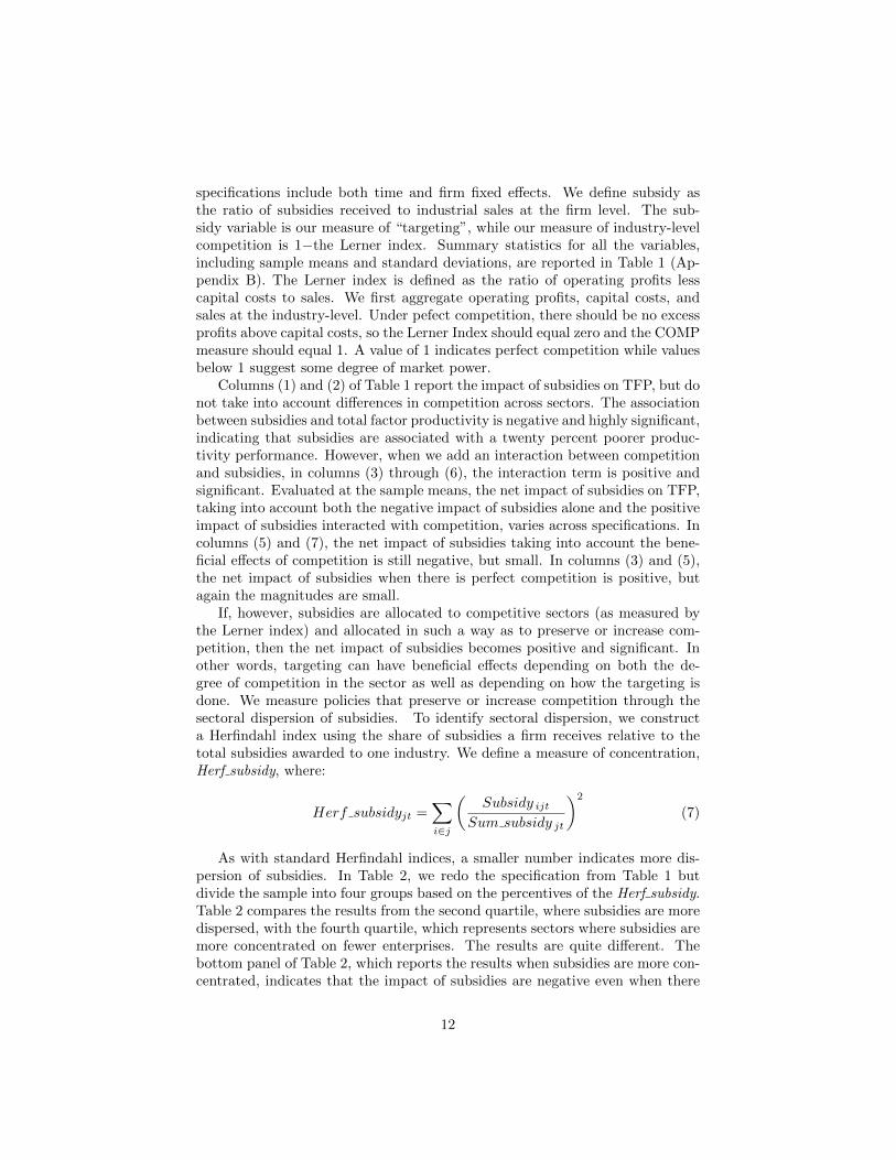
specifications include both time and firm fixed effects. We define subsidy asthe ratio of subsidies received to industrial sales at the firm level. The sub-sidy variable is our measure of “targeting”, while our measure of industry-levelcompetition is 1−the Lerner index. Summary statistics for all the variables,including sample means and standard deviations, are reported in Table 1 (Ap-pendix B). The Lerner index is defined as the ratio of operating profits lesscapital costs to sales. We first aggregate operating profits, capital costs, andsales at the industry-level. Under pefect competition, there should be no excessprofits above capital costs, so the Lerner Index should equal zero and the COMPmeasure should equal 1. A value of 1 indicates perfect competition while valuesbelow 1 suggest some degree of market power.

Columns (1) and (2) of Table 1 report the impact of subsidies on TFP, but donot take into account differences in competition across sectors. The associationbetween subsidies and total factor productivity is negative and highly significant,indicating that subsidies are associated with a twenty percent poorer produc-tivity performance. However, when we add an interaction between competitionand subsidies, in columns (3) through (6), the interaction term is positive andsignificant. Evaluated at the sample means, the net impact of subsidies on TFP,taking into account both the negative impact of subsidies alone and the positiveimpact of subsidies interacted with competition, varies across specifications. Incolumns (5) and (7), the net impact of subsidies taking into account the bene-ficial effects of competition is still negative, but small. In columns (3) and (5),the net impact of subsidies when there is perfect competition is positive, butagain the magnitudes are small.

If, however, subsidies are allocated to competitive sectors (as measured bythe Lerner index) and allocated in such a way as to preserve or increase com-petition, then the net impact of subsidies becomes positive and significant. Inother words, targeting can have beneficial effects depending on both the de-gree of competition in the sector as well as depending on how the targeting isdone. We measure policies that preserve or increase competition through thesectoral dispersion of subsidies. To identify sectoral dispersion, we constructa Herfindahl index using the share of subsidies a firm receives relative to thetotal subsidies awarded to one industry. We define a measure of concentration,Herf subsidy, where:

Herf subsidyjt =∑i∈j

(Subsidy ijt

Sum subsidy jt

)2

(7)

As with standard Herfindahl indices, a smaller number indicates more dis-persion of subsidies. In Table 2, we redo the specification from Table 1 butdivide the sample into four groups based on the percentives of the Herf subsidy.Table 2 compares the results from the second quartile, where subsidies are moredispersed, with the fourth quartile, which represents sectors where subsidies aremore concentrated on fewer enterprises. The results are quite different. Thebottom panel of Table 2, which reports the results when subsidies are more con-centrated, indicates that the impact of subsidies are negative even when there

12

is perfect competition in the sector. In column (6), for example, the sum of6.238 and −6.338 is negative. The top panel of Table 2, however, indicates thatthe net impact of subsidies is positive when there is perfect competition. Forexample, the net impact of subsidies in columns (3) and (5) is positive, andthe coefficients indicate that a one standard deviation increase in the level ofsubsidies would lead to an increase in productivity of .7 percentage points, usingthe coefficients in column (3).

Table 3 replaces the interaction of competition and subsides with our mea-sure of the dispersion of subsidies, which can be defined as the inverse of ourHerf subsidy term, or InvSubsidyHerf. To the extent that greater dispersion ofsubsidies within a sector induces greater focus by encouraging more firms to in-novate within a specific sector, we would expect the coefficient on that variableto positively affect productivity. The results in Table 3 show that this is indeedthe case. The coefficient on InvSubsidyHerf is positive and statistically signifi-cant. The coefficient estimates indicate that a one standard deviation increasein the variable leads to an increase in TFP of 1.4 percentage points.

While not reported here, the results presented in Tables 1 through 3 arequalitatively the same if we transform the equations into differences and estimatethe impact of changes in competition and subsidies on TFP growth. It shouldnot be surprising that the results are robust to taking first differences, as all thespecifications in Tables 1 through 3 include firm and year fixed effects. Next, inTables 4 and 5, we replace TFP as our performance measure with an alternativemeasure of innovation. We identify as our new measure the share of a firm’soutput value generated by new products. This new product ratio, which wedefine as ”Ratio newproduct“, is an alternative proxy for innovation by thefirm.

In Table 4, we report the results for all observations, with the dependentvariable Ratio newproduct. Competition as measured by the Lerner index issignificantly and positively associated with the share of new products in totalsales, and the subsidy is associated with a negative but insignificant impacton new products. The interaction term is insignificant across all specifications.Without taking into account targetting policies that preserve or enhance com-petition (which we measure using the dispersion of subsidies), the net impactof subsidies on the share of new products even in a competitive environment isnot statistically significant.

In Table 5, we separate the sample according to the dispersion of subsidies.As we saw in Table 2, the positive effects of subsidies are only apparent whenthere is both significant competition and significant dispersion, as proxied bythe inverse of the subsidy herf. The second quartile, which indicates greaterdispersion of subsidies, shows that while subsidies alone are associated witheither insignificant or negative effects on the share of new products in sales,when coupled with greater competition the impact is positive and significant.The net impact of subsidies when there is significant competition, as indicatedby the coefficients in column (6), suggest that a one standard deviation increasein subsidies is associated with a small net increase in the share of new productsin sales. However, in the fourth quartile, where subsidies are concentrated on

13

very few firms, there is no significant positive impact of subsidies on new productsales even when there is perfect competition.

The results in Tables 1 through 5 together indicate that innovation, as mea-sured by either total factor productivity or the share of new products in totalsales, is increasing with subsidies only when two conditions hold. First, theremust be sufficiently high competition, as measured by [1− Lerner index]. Sec-ond, how the promotion is done is equally important: promotion tools must besufficiently widespread across many firms.

One issue which could be raised is the potential endogeneity of targeting.What if targeting is applied to firms already likely to succeed? Conversely, whatif targeting is only for firms likely to fail, and is in fact a bailout or soft budgetconstraint masquerading as industrial policy? In the former case, we are likelyto over-state the benefits of industrial policy, while in the latter case we arelikely to under-estimate them. In the next section, we propose one approach toaddress potential endogeneity.

3.4 Addressing endogeneity: an alternative specification

In this part, we propose an alternative approach to understanding the impor-tance of competition and focus in making industrial policy work. In particular,we test whether a pattern of subsidies focused on more competitive sectors,using the pattern of competition across different industrial sectors at the begin-ning of the sample period, explains differential success of industrial policies. Wethen introduce an alternative targeting measure, tariffs, which address some ofthe endogeneity concerns at the firm level because they are set nationally.

We begin by measuring the pattern of subsidies at the city-year level, em-ploying one method developed in Nunn and Trefler (2010). To test whethersubsidies are more effective when introduced in a competitive setting, we pro-pose to measure the correlation of subsidies with competition and then seewhether the strength of that correlation raises firm performance. To measurewhether subsidies are biased towards more competitive sectors in city r in yeart , we calculate the correlation between the industry-city level initial degree ofcompetition and current period t subsidies in sector j and city r :

Ωrt = Corr(SUBSIDYrjt, COMPETITIONrj0) (8)

Since subsidies vary over time, we have a time-varying change in the correla-tion between initial levels of competition and the patterns of interventions. Wethen explore whether higher correlations between subsidies and competition, asmeasured by Ωrt, were associated with better performance. Total factor pro-ductivity is computed using four methods: AW et al 2001 (AW), OLS, OLS withfixed effects, and Olley & Pakes 1996 (OP). The firm-level estimation equationis as follows:

lnTFPijrt = α0 + α1Ωrt + α2SUBSIDYijt−1 + α3Xijrt + αi + αt + εijt (9)

TFPijrt is the total factor productivity for firm i in industry j located in cityr in year t . SUBSIDYijt−1 is the level of subsidy for firm i in sector j and

14

region r in year t − 1. Xijrt includes firm level controls such as the share ofthe firms’ total equity owned by the state, etc. fi is firm fixed effects and Dt

represents year dummies.To check the impact of targeting on industry level performance, which takes

into account both within-firm changes in behavior as well as reallocation acrossfirms, we also compute aggregate industry productivity measures for each cityevery year and estimate the following equation:

lnTFPjrt = α0 + α1Ωrt + α2SUBSIDYjt−1 + α3Xjrt + αi + αt + εijt (10)

In a given city and year the aggregate industry productivity measure lnTFPjrt isa weighted average of the firm’s individual un-weighted productivities lnTFPijrtwith an individual firm’s weight sit corresponding to its output’s share in totalindustry output in a particular year and city:

lnTFPjrt =∑i

sit lnTFPijrt (11)

In the industry-level equation, Xjrt includes industry-city level controls, ηj andhr are industry fixed effects and region dummies, respectively, and Dt includesyear dummies.

The coefficient on the subsidy term captures the own firm or own industryeffect of the policy on total factor productivity. The coefficient on the correla-tion coefficient between subsidies and competition indicates the beneficial effectof targeting, at the city level, when such targeting via subsidies is higher incompetitive industries, as measured by the initial degree of competition at thebeginning of the sample period.

Table 6 presents results for estimation equation (9). Columns (1) to (3)show firm-level estimation results using OLS, OLS with firm fixed effects, andOLS when TFP is calculated using the Olley-Pakes approach. All specificationsinclude year and firm fixed effects. These results show that while the individ-ual effects of subsidies at the firm level is associated with a negative impacton TFP, a positive correlation coefficient between the pattern of subsidizationand competition is associated with a positive and significant impact on firmproductivity. The coefficient estimate in column (3), .072, indicates that if thecorrelation between subsidies and competition at the city level was perfect (100percent), then productivity would be 7.2 percent higher. Based on the samplemeans, a one standard deviation increase in the city-industry correlation wouldincrease TFP by 0.6 percentage points for firms in that city and industry.

Table 7 separates the sample by the dispersion of subsidies, using the Herf-subsidy variable defined earlier. The impact of subsidies in the second quartile(when subsidies are more dispersed) are reported in in the top panel of Table 7and the impact in the fourth quartile (when subsidies are more concentrated) isreported in the bottom panel. In the top panel, the coefficient on the correlationbetween subsidies and competition is positive, significant, and twice the size ofthe coefficient in Table 6. The coefficient estimate, at 0.145 in the third column,indicates that perfect correlation between subsidies given and competition levels

15

would increase productivity by 14.5 percentage points. The coefficient on sub-sidies alone, while still negative, is barely significant at conventional levels. Thenet impact of a one standard deviation increase in subsidies and the correlationvariable would lead to a net increase in productivity of 1.2 percentage points.In contrast, the bottom panel of Table 7 shows no significant positive effectsof the correlation measure. The results in Table 7 indicate that when subsidiesare not sufficiently disbursed across firms, then subsidies do not positively af-fect productivity even when subsidies are higher in more competitive sectors.These results confirm the earlier results in Tables 1 and 2 suggesting that bothcompetition and focus are necessary to promote industrial performance.

Tables 8 and 9 repeat the specifications reported in Tables 6 and 7 butestimate (10) instead, where the firm-level measure of the log of total factorproductivity is replaced with the share-weighted industry-level measure as de-fined above. The results are comparable at the industry level to those at thefirm-level, indicating that the benefits of industrial policy when there is compe-tition and focus survive at the aggregate level.

Another approach to addressing the endogeneity of subsidies is to redo theanalysis using an instrument of industrial policy which does not vary acrossfirms. One such instrument is tariffs, which protect all firms in a particularsector. Consequently, we redid the estimation, but replaced subsidies with tariffsand replaced the correlation between initial competition and subsidies with thecorrelation between initial competition and current period tariffs. At the citylevel, the correlation between that city’s degree of competition at the beginningof the sample period and current period tariffs should be strictly exogenous, asthe level of competition is predetermined and tariffs are set at the national, notthe city, level. Our new correlation measure is now defined as:

Ωrt = Corr(TARIFFjt, COMPETITIONrj0) (12)

The results are reported in Tables 10 and 11. In Table 10, the coefficient onthe correlation measure defined in (12) is positive and statistically significantacross all specifications. The coefficient, which ranges from .0722 to .0833,indicates that a perfect (100 percent) correlation between higher tariff levelsin sector j and time t and the degree of competition in region r, sector j andthe initial year would lead to an increase in productivity of 7 to 8 percentagepoints. However, the independent effect of tariffs on productivity is negative andsignificant, as indicated by the coefficient on lnTariff lag. Evaluated using aone standard deviation increase in both variables from Appendix Table 1, thenet impact of an increase in tariffs is likely to be negative. In Table 11, werepeat the analysis using industry-level variables, which takes into account notonly within firm changes in productivity but productivity gains or losses fromreallocating market shares across firms. The results are qualitatively similar,but the negative impact of tariffs on productivity are stronger and larger inmagnitude. Unless the targeting of tariffs is significantly stronger, with a highercorrelation between the degree of competition in a sector and sectoral tarifflevels, the negative impact of tariffs (possibly due to their anti-competitive

16

effect) is likely to predominate. This is in contrast to subsidies, which theresults indicate do have a net positive effect when we take into account thepositive impact of targeting more competitive sectors.

Future extensions will further explore alternative ways to address the poten-tial endogeneity of firms targeted for industrial policy. In particular, we haverecently purchased a dataset on roads in China over time and across provincesto use as a potential instrument for our measures of competition.

4 Conclusion

In this paper we have argued that sectoral state aids tend to foster productivity,productivity growth, and product innovation to a larger extent when it targetsmore competitive sectors and when it is not concentrated on one or a smallnumber of firms in the sector. A main implication from our analysis is thatthe debate on industrial policy should no longer be for or against having such apolicy. As it turns out, sectoral policies are being implemented in one form oranother by a large number of countries worldwide, starting with China. Rather,the issue should be on how to design and govern sectoral policies in order tomake them more competition-friendly and therefore more growth-enhancing.While our analysis suggests that proper selection criteria together with goodguidelines for governing sectoral support, can make a significant difference interms of growth and innovation performance, yet the issue remains of how tominimize the scope for influence activities by sectoral interests when a sectoralstate aid policy is to be implemented. One answer is that the less concentratedand more competition-compatible the allocation of state aid to a sector, theless firms in that sector will lobby for that aid as they will anticipate lowerprofits from it. In other words, political economy considerations should reinforcethe interaction between competition and the efficiency of sectoral state aid. Acomprehensive analysis of the optimal governance of sectoral policies still awaitsfurther research.

References

[1] Aghion, Philippe, Bloom, Nick, Blundell, Richard, Griggith, Rachel andHowitt, Peter (2005), “PeterCompetition and Innovation: An Inverted-URelationship,” Quarterly Journal of Economics, vol. 120(2), pages 701-728.

[2] Beck, Thorsten, Demirguc-Kunt, Asli and Levine, Ross (2000), “A NewDatabase on Financial Development and Structure,” World Bank EconomicReview 14, 597-605, (November 2010 update).

[3] Brander, James A. (1995), “Strategic Trade Policy,” NBER Working Pa-pers 5020, National Bureau of Economic Research, Inc.

17

[4] Brander, James A. and Spencer, Barbara J. (1985), “Export Subsidies andInternational Market Share Rivalry,” Journal of International Economics,vol. 18(1-2), pages 83-100.

[5] Greenwald, Bruce and Stiglitz, Joseph E. (2006), “Helping InfantEconomies Grow: Foundations of Trade Policies for Developing Countries,”American Economic Review, vol. 96(2), pages 141-146.

[6] Griliches, Zvi and Mairesse, Jacques (1995), “Production Functions: TheSearch for Identification”, NBER Working Paper No. 5067 .

[7] Harrison, Ann (1994), “An Empirical Test of the Infant Industry Argument:Comment”, American Economic Review, vol. 84, 4, pages 1090-1095.

[8] Harrison, Ann and Rodrıguez-Clare, Andres (2009), “Trade, Foreign In-vestment, and Industrial Policy for Developing Countries,” NBER WorkingPapers 15261, National Bureau of Economic Research, Inc.

[9] Hausmann, Ricardo and Rodrik, Dani (2003), “Economic development asself-discovery,” Journal of Development Economics, vol. 72(2), pages 603-633.

[10] Krueger, Anne O. and Tuncer, Baran (1982), “An Empirical Test of theInfant Industry Argument,” American Economic Review, vol. 72(5), pages1142-52.

[11] Nunn, Nathan and Trefler, Daniel (2010), “The Structure of Tariffs andLong-Term Growth,” American Economic Journal: Macroeconomics, vol.2(4), pages 158-94.

[12] Olley, Steven and Pakes, Ariel (1996,. “The Dynamics of productivity inthe Telecommunications Equipment Industry”, Econometrica, 64, pages1263-1297.

[13] Rodrik, Dani (1999), Making Openness Work: The New Global Economyand the Developing Countries, Barnes and Noble, Washington DC.

A Appendix: Theory

A.1 Social Optimum

In this first part of the Appendix we assume full Bertrand competition withinsectors, and then compare the laissez-faire choice between diversity and focuswith the choice that maximizes social welfare, not just innovation intensity andgrowth.

Suppose that a social planner could impose targeting on a single tevchnol-ogy, i.e.,force the two firms to focus on that same technology. The benefit ofsociety from targeting on technology A is to provide a larger cost decrease fromproduction and also a lower price for consumers. Hence targeting is necessarily

18

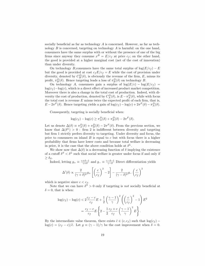
socially beneficial as far as technology A is concerned. However, as far as tech-nology B is concerned, targeting on technology A is harmful: on the one hand,consumers have the same surplus with or without the presence of one of the bigfirms since anyway they consume xB = E/cf at price cf ; on the other hand,the good is provided at a higher marginal cost (net of the cost of innovation)than under diversity.

On technology B,consumers have the same total surplus of log(E/cf ) − Ebut the good is provided at cost cfE/cf = E while the cost of provision underdiversity, denoted by CDB (δ), is obviously the revenue of the firm, E, minus itsprofit, πDB (δ). Hence targeting leads a loss of πDB (δ) on technology B.

On technology A, consumers gain a surplus of log(E/c) − log(E/cf ) =log(cf )−log(c), which is a direct effect of increased product market competition.Moreover there is also a change in the total cost of production. Indeed, with di-versity the cost of production, denoted by CDA (δ), is E−πDA (δ), while with focusthe total cost is revenue E minus twice the expected profit of each firm, that is,E− 2πF (δ). Hence targeting yields a gain of log(cf )− log(c) + 2πF (δ)− πDA (δ).

Consequently, targeting is socially beneficial when:

log(cf )− log(c) ≥ πDA (δ) + πDB (δ)− 2πF (δ).

Let us denote ∆(δ) ≡ πDA (δ) + πDB (δ) − 2πF (δ). From the previous section, weknow that ∆(δL) > 0 : firm 2 is indifferent between diversity and targetingbut firm 1 strictly prefers diversity to targeting. Under diversity and focus, theprice to consumers on island B is equal to c but with focus there is a higherprobability that firms have lower costs and because total welfare is decreasingin price, it is the case that the above condition holds at δL.

We show now that ∆(δ) is a decreasing function of δ implying the existenceof a cutoff δS < δL such that social welfare is greater under focus if and only if≥ δS .

Indeed, letting g+ ≡ γ+δ−1γ+δ and g− ≡ γ−δ−1

γ−δ Direct differentiation yields

∆′(δ) ∝ 2

(γ + δ)2g+

[(c

cf

)2

− 2

]− 2

(γ − δ)2g−

(c

cf

)2

which is negative since c < cf .Note that we can have δS > 0 only if targeting is not socially beneficial at

δ = 0, that is when:

log(cf )− log(c) < 2cf − ccf

E +1

2

(γ − 1

γ

)2((

c

cf

)2

− 1

)E2

=cf − ccf

E

2− 1

2

cf + c

cf

(γ − 1

γ

)2

E

.

By the intermediate value theorem, there exists c ∈ (c, cf ) such that log(cf ) −log(c) = (cf − c)/c. Let g ≡ (γ − 1)/γ be the cost improvement when δ = 0.

19

The condition becomes:

1

2

cf + c

cfg2E2 − 2E +

cfc< 0. (13)

The discriminant of the quadratic is 1 − (cf + c)g2/(2c) < 0. Therefore, ifg2 > c/(cf + c) there is no real root, and δS = 0. However if g2 < c/(cf + c),there exist two roots for the quadratic equation.6

For instance, if γ = 1, there is no cost improvement (g = 0) and the conditionis that E ∈ [0, 2cf/(cf + c)]; if g2 = c/(cf + c), the condition cannot be satisfiedfor any value of E. We summarize our findings in the following proposition.

Proposition 2 1. There exists δS < δL such that targeting is socially opti-mal if, and only if, δ is greater than δS.

2. Letting g = γ−1γ , δS = 0 when g2 ≥ 1

2c

cf+c.

3. When g2 < ccf+c

, there exist E0, E1 with E0 < E1 such that δS > 0 only

if the market size E ∈ [E0, E1]; for E < E0 or E > E1, δS = 0

These results are quite intuitive. First, ceteris paribus, for small valuesof δ, targeting has a low social benefit (in terms of higher competition andinnovation) relative to the cost reduction on technology B achieved thanks todiversity. There may however be room for a targeting policy for higher δ’s: thedesire to relax price competition by choosing diversity leads the big firms notto focus enough.

Second, with perfect information, (innovation-reducing) diversity is welfare-decreasing if γ, and thus the potential cost decrease from innovation, is highenough. In this case, laissez-faire conflicts with social optimal for all values of δless than δL, and we can ‘safely’ go for targeting: it is either welfare-increasing(for δ < δL) or irrelevant (for δ ≥ δL).

Third, for smaller values of γ, there exists a intermediate region for marketsize E, where diversity may be socially optimal for some values of δ. If marketsize (E) is large, targeting is desirable.

A.2 Imperfect Information

Our assumption of perfect information is obviously extreme. Below we considertwo possibilities. One where the firms know the technology on which the costreduction possibilities are greater but the planner does not. The other case iswhere neither the firms nor the planner know the identity of the technologywith the greater cost reduction. It turns out that the first case is equivalentto the case of perfect information if the planner can use mechanisms. For thesecond case, the laissez-faire outcome looks very different from the one underperfect information since it is now for high values of δ that diversity emerges.

6The roots are E0 = 2cf1−

√1−

cf+c

2cg2

cf+c, E1 = 2cf

1−√

1+cf+c

2cg2

cf+c.

20

The possibility of conflict between the firms and the planner are still presentand there is value for a targeting policy.

A.2.1 Only the planner has imperfect information

If the planner has imperfect information about the identity of the technologyleading to higher cost reduction but the firms (or at least one of them) haveperfect information, as long as δ is known by the planner, the perfect informationoutcome can be replicated.

For δ ≥ δS , letting the firm diversify is socially optimal and the planner willnot intervene. When δ < δS , the planner would like to impose targeting on thebetter technology, but it does not know which one it is. However, conditional onbeing obliged to focus, firms 1 and 2 prefer to do it on the better technology,so that a planner can simply impose targeting to firms 1, 2 and let them locatesubject to this constraint.

If in addition the planner does not have information about the value ofδ, since the parties have correlated information revelation mechanisms can beused to extract this information from the parties. The design of the optimalmechanism is beyond the scope of this paper however.

A.2.2 All parties have imperfect information

When neither the firms nor the planner have information about which tech-nology leads to the higher cost reduction under innovation, there may be acoordination failure both under laissez-faire and under intervention.

We consider the case where firms locate without knowing whether the marketthey have chosen allows for a cost reduction of γ + δ or γ − δ but, upon beingcalled to innovate, they learn which cost reduction can be generated. Thisinterpretation facilitates comparison with the perfect-information case.

Assume first diversity. Then total industry profit is the same as before sincefirms make the same decisions when they are chosen to innovate.

Under focus, since at the time technology is chosen firms do not know whichis the beter one, focus yields with probability 1/2 the level of profit πF (δ) andwith probability 1/2 the same level of profit but with γ + δ replaced by γ − δ ,that is, 1

2 (πF (δ) + πF (−δ)).By revealed preferences in the perfect information case, we have πD(δ) >

πF (δ) since a firm under diversity could have chosen to set the same price anduse the same innovation intensity as under focus. A similar argument showsthat πD(−δ) > πF (−δ), therefore:

(πD(δ) + πD(−δ))/2 > (πF (δ) + πF (−δ))/2

and firms prefer to diversity rather than to focus for any value of δ.

Proposition A1 Under imperfect information, the laissez-faire outcome is forfirms to diversify for any value of δ and γ.

21

Let us now turn to intervention. Diversity brings the same social value asunder perfect information. With targeting on the good technology, the socialbenefit is the same as under perfect information; but the social benefit is muchlower than under perfect information with targeting on the bad technology.When there is focus, the total cost is in fact 1

2 (2E − πF (δ) − πF (−δ)) andtherefore targeting is socially optimal when:

log(cf )− log(c) ≥ πD(δ) + πD(−δ)− (πF (δ) + πF (−δ)).

The RHS is the difference in industry profit between diversity and focus,which is positive by Proposition A1. Using the expressions for the profit func-tions, we have:

πD(δ) + πD(−δ)− (πF (δ) + πF (−δ))

=1

4

[(γ + δ − 1

γ + δ

)2

+

(γ − δ − 1

γ − δ

)2]((

c

cf

)2

− 1

)E2 + 2

cf − ccf

E.

We know from the derivations in section 2.4 that the term in brackets is de-creasing in δ; since c < cf , the coefficient of E2 is negative and therefore theexpression is increasing in δ. This is in sharp contrast with the perfect infor-mation case since the difference in industry profit between diversity and focuswas decreasing in δ. In the perfect information case, focusing on the “good”technology led to a decreasing opportunity cost since as δ increases the value ofbeing located on the “bad” technology sector decreases. With imperfect infor-mation though, focusing makes it as likely to be on competition in the “good”or in the“bad” sector; since conditional on being on one sector firms prefer notto face competition as δ increases, firms value more diversity.

A necessary condition for targeting to be socially optimal is that log(cf ) −log(c) be greater than the minimum difference in profits, which arises at δ = 0,which is the case where both technologies yield the same cost reduction in thecase of innovation. Using the same reasoning as in the perfect information casefor deriving condition (13), if c solves log(cf )− log(c) = (cf − c)/c the necessarycondition can be written when δ = 0 as (recall that g ≡ (γ − 1)/γ):

cf + c

cfg2E2 − 2E +

cfc> 0

which is (obviously) the same condition as under perfect information. Thereforewhen g2 is larger than c/(cf + c), targeting is optimal when δ = 0 and when g2

is smaller than this value, targeting is optimal when E is smaller than the rootE0 or is larger than the root E1.

If focus is optimal at δ = 0, by continuity there exists δ∗ > 0 such that focusis socially optimal for all δ less than δ∗.

Proposition A2 1. If g2 > ccf+c

, there exists δ∗ > 0 such that targeting is

socially optimal for all δ < δ∗.

2. If g2 < ccf+c

, and E < E0 or E > E1, there exists δ∗∗ > 0 such that

targeting is socially optimal for all δ < δ∗∗.

22

3. If g2 < ccf+c

, and E ∈ [E0, E1] targeting is not an optimal policy for all

values of δ.

Because targeting under imperfect information yields a smaller surplus thanunder perfect information while diversity brings the same benefit, it must be thecase that focus is less often socially optimal, and therefore δ∗ is strictly smallerthan the cutoff δS in Proposition 2.

Finally, one can show that δ∗ > δ∗∗, so that, as in the perfect informationcase, the range of δ’s for which targeting is socially optimal, is bigger when thegrowth rate g is high than when it is low. To prove that claim, it suffices tonote that if:

∆Π = πD(δ) + πD(−δ)− (πF (δ) + πF (−δ)),

we have:∂∆Π

∂δ> 0;

∂∆Π

∂γ< 0.

To see this, note that:

∆Π ≈ −

[(γ + δ − 1

γ + δ

)2

+

(γ − δ − 1

γ − δ

)2]

≡ −F (δ, γ),

where:∂F

∂δ=

1

(γ + δ)2− 1

(γ + δ)3− 1

(γ − δ)2+

1

(γ + δ)3< 0

and:∂F

∂γ=

(1− 1

γ + δ

)1

(γ + δ)2+

(1− 1

γ − δ

)1

(γ − δ)2> 0.

A.3 Growth and dynamic welfare under focus versus di-versity

Consider a dynamic extension of the model where the social planner seeks tomaximize intertemporal utility

U =

∞∑t=1

(1 + r)−t[log xAt + log xBt

],

although private consumers and entrepreneurs live for one period only. More-over, assume that, due to knowledge spillovers, after one period all firms multiplytheir initial productivity by the same γ ∈ γ + δ, γ − δ as the innovative firm.Then a social planner who wants to maximize intertemporal utility, will takeinto account not only the static welfare analyzed above, but also the averagegrowth rates respectively under diversity and under focus.

23

The growth rates of utility under diversity and focus, are respectively givenby:

GD =

[1

2

(1− 1

γ + δ

)log(γ + δ) +

1

2

(1− 1

γ − δ

)log(γ − δ)

]c

cfE

and

GF =

(1− 1

γ + δ

)log(γ + δ)E.

We clearly haveGF > GD,

as a results of two effects that play in the same direction: (i) focus increasesthe expected size of innovation (always equal to log(γ + δ) under focus, butsometimes equal to log(γ− δ) under diversity); (ii) focus increases the expectedfrequency of innovation both because innovation under focus induces biggercost reduction under focus (under diversity cost is sometimes reduced by factor(γ − δ)) and because under focus there is more incentive to innovate in orderto escape competition (term c

cfin the expression for GD). This immediately

establishes:

Proposition A3 There exists a cut-off value δS(r) < δS , increasing in r, suchthat focus maximizes dynamic welfare whenever δ > δS(r).

24

B Appendix: Tables

25

Table 1Table 1Table 1Table 1Table 1Table 1Table 1 (1) (2) (3) (4) (5) (6)

Dependent: lnTFP (based on Olley-Pakes regression)Dependent: lnTFP (based on Olley-Pakes regression)Dependent: lnTFP (based on Olley-Pakes regression)Dependent: lnTFP (based on Olley-Pakes regression)Dependent: lnTFP (based on Olley-Pakes regression)Dependent: lnTFP (based on Olley-Pakes regression)Dependent: lnTFP (based on Olley-Pakes regression)Stateshare -0.00150 -0.00144 -0.00159 -0.00152 -0.00185 -0.00179

(0.00337) (0.00331) (0.00337) (0.00331) (0.00329) (0.00326)Horizontal 0.322*** 0.335*** 0.323*** 0.335*** 0.178* 0.198*

(0.0756) (0.0793) (0.0755) (0.0793) (0.0947) (0.101)Ratio_subsidy -0.185*** -0.188*** -8.201*** -6.752*** -8.067*** -6.798***

(0.0279) (0.0276) (1.769) (1.404) (1.748) (1.392)Competition_lerner 0.512 0.482 0.427

(0.533) (0.535) (0.535)Interaction_lerner 8.212*** 6.724*** 8.074*** 6.773***

(1.818) (1.441) (1.796) (1.429)Backward 0.779*** 0.762***

(0.278) (0.273)Forward 0.112 0.0995

(0.0991) (0.0990)LnTariff -0.0382** -0.0348** -0.0380** -0.0348** -0.0335 -0.0321

(0.0162) (0.0166) (0.0162) (0.0166) (0.0214) (0.0213)LnbwTariff -0.00764 -0.00672 -0.00770 -0.00682 -0.0223 -0.0213

(0.0174) (0.0172) (0.0174) (0.0172) (0.0194) (0.0189)LnfwTariff -0.00373 -0.00422 -0.00379 -0.00424 -0.00418 -0.00406

(0.00260) (0.00278) (0.00260) (0.00278) (0.00544) (0.00537)Constant 1.726*** 1.213** 1.725*** 1.242** 1.699*** 1.274**

(0.0315) (0.534) (0.0314) (0.535) (0.0412) (0.533)Observations 1,072,034 1,072,034 1,072,034 1,072,034 1,072,034 1,072,034R-squared 0.172 0.172 0.172 0.173 0.173 0.173Notes: Robust clustered standard errors are shown in the parenthesis. Firm fixed effect and time effect are included in each specification. Notes: Robust clustered standard errors are shown in the parenthesis. Firm fixed effect and time effect are included in each specification. Notes: Robust clustered standard errors are shown in the parenthesis. Firm fixed effect and time effect are included in each specification. Notes: Robust clustered standard errors are shown in the parenthesis. Firm fixed effect and time effect are included in each specification. Notes: Robust clustered standard errors are shown in the parenthesis. Firm fixed effect and time effect are included in each specification. Notes: Robust clustered standard errors are shown in the parenthesis. Firm fixed effect and time effect are included in each specification. Notes: Robust clustered standard errors are shown in the parenthesis. Firm fixed effect and time effect are included in each specification.

Table 2 Table 2 Table 2 Table 2 Table 2 Table 2 Table 2 (1) (2) (3) (4) (5) (6)

Dependent: lnTFP (based on Olley and Pakes regression) Dependent: lnTFP (based on Olley and Pakes regression) Dependent: lnTFP (based on Olley and Pakes regression) Dependent: lnTFP (based on Olley and Pakes regression) Dependent: lnTFP (based on Olley and Pakes regression) Dependent: lnTFP (based on Olley and Pakes regression) Dependent: lnTFP (based on Olley and Pakes regression) The second quartile: more dispersion in subsidies The second quartile: more dispersion in subsidies The second quartile: more dispersion in subsidies The second quartile: more dispersion in subsidies The second quartile: more dispersion in subsidies The second quartile: more dispersion in subsidies The second quartile: more dispersion in subsidies

Ratio_subsidy -0.197* -0.193** -16.25*** -12.00*** -16.49*** -11.96*** (0.0962) (0.0937) (4.884) (4.037) (4.813) (4.031)

Competition_lerner 1.818 1.763 2.001 (1.286) (1.285) (1.308)

Interaction_lerner 16.63*** 12.24*** 16.88*** 12.19*** (5.096) (4.186) (5.023) (4.178)

The fourth quartile: least dispersion in subsidies (most concentrated) The fourth quartile: least dispersion in subsidies (most concentrated) The fourth quartile: least dispersion in subsidies (most concentrated) The fourth quartile: least dispersion in subsidies (most concentrated) The fourth quartile: least dispersion in subsidies (most concentrated) The fourth quartile: least dispersion in subsidies (most concentrated) The fourth quartile: least dispersion in subsidies (most concentrated) Ratio_subsidy -0.227*** -0.228*** -9.352** -6.169** -9.148** -6.338**

(0.0625) (0.0627) (3.615) (2.854) (3.710) (2.860) Competition_lerner 1.179 1.153 1.029

(0.981) (0.982) (1.042) Interaction_lerner 9.320** 6.069** 9.107** 6.238**

(3.628) (2.883) (3.727) (2.888)

Horizontal Yes Yes Yes Yes Yes Yes Forward & Backward No No No No Yes Yes Tariffs Yes Yes Yes Yes Yes Yes

Table 3Table 3Table 3Table 3Table 3Table 3Table 3 (1) (2) (3) (4) (5) (6)

Dependent: lnTFP (based on Olley-Pakes regression)Dependent: lnTFP (based on Olley-Pakes regression)Dependent: lnTFP (based on Olley-Pakes regression)Dependent: lnTFP (based on Olley-Pakes regression)Dependent: lnTFP (based on Olley-Pakes regression)Dependent: lnTFP (based on Olley-Pakes regression)Dependent: lnTFP (based on Olley-Pakes regression)Stateshare -0.00150 -0.00106 -0.00144 -0.00106 -0.00171 -0.00133

(0.00337) (0.00322) (0.00331) (0.00322) (0.00326) (0.00317)Horizontal 0.322*** 0.343*** 0.335*** 0.343*** 0.198* 0.212**

(0.0756) (0.0785) (0.0793) (0.0785) (0.101) (0.0975)Ratio_subsidy -0.185*** -0.200*** -0.188*** -0.200*** -0.187*** -0.199***

(0.0279) (0.0320) (0.0276) (0.0320) (0.0277) (0.0318)Competition_lerner 0.448 0.512 0.448 0.457 0.399

(0.542) (0.533) (0.542) (0.534) (0.543)Competition_HerfSubsidy 0.000177*** 0.000177*** 0.000170**

(6.24e-05) (6.24e-05) (6.49e-05)Backward 0.762*** 0.738***

(0.273) (0.274)Forward 0.0992 0.0931

(0.0990) (0.101)lnTariff -0.0382** -0.0360** -0.0348** -0.0360** -0.0322 -0.0338*

(0.0162) (0.0155) (0.0166) (0.0155) (0.0213) (0.0202)lnbwTariff -0.00764 -0.00578 -0.00672 -0.00578 -0.0212 -0.0199

(0.0174) (0.0166) (0.0172) (0.0166) (0.0189) (0.0186)lnfwTariff -0.00373 -0.00556** -0.00422 -0.00556** -0.00402 -0.00517

(0.00260) (0.00276) (0.00278) (0.00276) (0.00537) (0.00541)Constant 1.726*** 1.311** 1.213** 1.311** 1.245** 1.337**

(0.0315) (0.539) (0.534) (0.539) (0.532) (0.537)

Observations 1,072,034 1,072,034 1,072,034 1,072,034 1,072,034 1,072,034R-squared 0.172 0.173 0.172 0.173 0.173 0.174

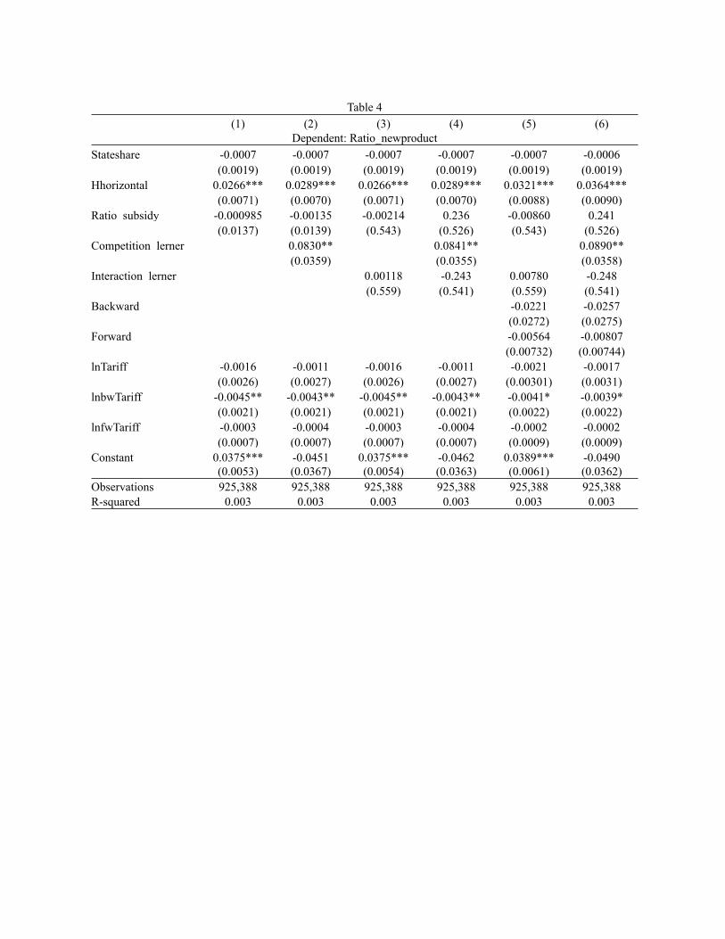
Table 4 Table 4 Table 4 Table 4 Table 4 Table 4 Table 4 (1) (2) (3) (4) (5) (6)

Dependent: Ratio_newproductDependent: Ratio_newproductDependent: Ratio_newproductDependent: Ratio_newproductDependent: Ratio_newproductDependent: Ratio_newproductDependent: Ratio_newproductStateshare -0.0007 -0.0007 -0.0007 -0.0007 -0.0007 -0.0006

(0.0019) (0.0019) (0.0019) (0.0019) (0.0019) (0.0019)Hhorizontal 0.0266*** 0.0289*** 0.0266*** 0.0289*** 0.0321*** 0.0364***

(0.0071) (0.0070) (0.0071) (0.0070) (0.0088) (0.0090)Ratio_subsidy -0.000985 -0.00135 -0.00214 0.236 -0.00860 0.241

(0.0137) (0.0139) (0.543) (0.526) (0.543) (0.526)Competition_lerner 0.0830** 0.0841** 0.0890**

(0.0359) (0.0355) (0.0358)Interaction_lerner 0.00118 -0.243 0.00780 -0.248

(0.559) (0.541) (0.559) (0.541)Backward -0.0221 -0.0257

(0.0272) (0.0275)Forward -0.00564 -0.00807

(0.00732) (0.00744)lnTariff -0.0016 -0.0011 -0.0016 -0.0011 -0.0021 -0.0017

(0.0026) (0.0027) (0.0026) (0.0027) (0.00301) (0.0031)lnbwTariff -0.0045** -0.0043** -0.0045** -0.0043** -0.0041* -0.0039*

(0.0021) (0.0021) (0.0021) (0.0021) (0.0022) (0.0022)lnfwTariff -0.0003 -0.0004 -0.0003 -0.0004 -0.0002 -0.0002

(0.0007) (0.0007) (0.0007) (0.0007) (0.0009) (0.0009)Constant 0.0375*** -0.0451 0.0375*** -0.0462 0.0389*** -0.0490

(0.0053) (0.0367) (0.0054) (0.0363) (0.0061) (0.0362)Observations 925,388 925,388 925,388 925,388 925,388 925,388R-squared 0.003 0.003 0.003 0.003 0.003 0.003

Table 5Table 5Table 5Table 5Table 5Table 5Table 5

(1) (2) (3) (4) (5) (6) Dependent: Ratio_newproduct Dependent: Ratio_newproduct Dependent: Ratio_newproduct Dependent: Ratio_newproduct Dependent: Ratio_newproduct Dependent: Ratio_newproduct Dependent: Ratio_newproduct

The second quartile The second quartile The second quartile The second quartile The second quartile The second quartile The second quartile Ratio_subsidy 0.00397 0.0036 -1.503* -1.689** -1.508* -1.679**

(0.0390) (0.0388) (0.821) (0.755) (0.816) (0.755) Competition_lerner -0.0724 -0.0798 -0.0777

(0.0789) (0.0780) (0.0720) Interaction_lerner 1.562* 1.755** 1.568* 1.744**

(0.841) (0.780) (0.837) (0.780) The fourth quartile The fourth quartile The fourth quartile The fourth quartile The fourth quartile The fourth quartile The fourth quartile

Ratio_subsidy 0.00185 0.00092 -1.324 -1.029 -1.332 -1.022 (0.0351) (0.0352) (1.475) (1.442) (1.468) (1.432)

Competition_lerner 0.117* 0.114* 0.122* (0.0662) (0.0657) (0.0622)

Interaction_lerner 1.359 1.057 1.368 1.049 (1.503) (1.470) (1.495) (1.460)

Horizontal Yes Yes Yes Yes Yes Yes Forward & Backward No No No No Yes Yes Tariffs Yes Yes Yes Yes Yes Yes

Table 6 Effect of Correlation (subsidy and lerner index) on Firm-level productivityTable 6 Effect of Correlation (subsidy and lerner index) on Firm-level productivityTable 6 Effect of Correlation (subsidy and lerner index) on Firm-level productivityTable 6 Effect of Correlation (subsidy and lerner index) on Firm-level productivityDependent: Firm-level TFP Dependent: Firm-level TFP Dependent: Firm-level TFP Dependent: Firm-level TFP

TFP_ols TFP_olsFE TFP_OPCor_subsidy_lerner 0.0325 0.0791*** 0.0720***

(0.0204) (0.0193) (0.0193)Stateshare -0.00265 -0.00178 -0.00347

(0.00386) (0.00365) (0.00366)Horizontal 0.201** 0.187* 0.189*

(0.0939) (0.0978) (0.0969)Backward 0.744*** 0.735*** 0.733***

(0.269) (0.272) (0.270)Forward 0.0900 0.104 0.103

(0.101) (0.0986) (0.0984)Subsidy_lag (at firm level) -0.0374 -0.0666** -0.0656**

(0.0252) (0.0257) (0.0263)Lerner_lag 0.00756 -0.139 -0.129

(0.105) (0.109) (0.108)lnTariff -0.0390* -0.0369* -0.0366*

(0.0224) (0.0215) (0.0219)lnbwTariff -0.0205 -0.0153 -0.0164

(0.0197) (0.0189) (0.0190)lnfwTariff -0.00273 -0.00278 -0.00287

(0.00531) (0.00511) (0.00511)Constant 0.973*** 1.932*** 1.729*** (0.111) (0.113) (0.113)Firm FEs yes yes yesYear dummies yes yes yesObservations 727,460 727,460 727,460R-squared 0.136 0.179 0.167

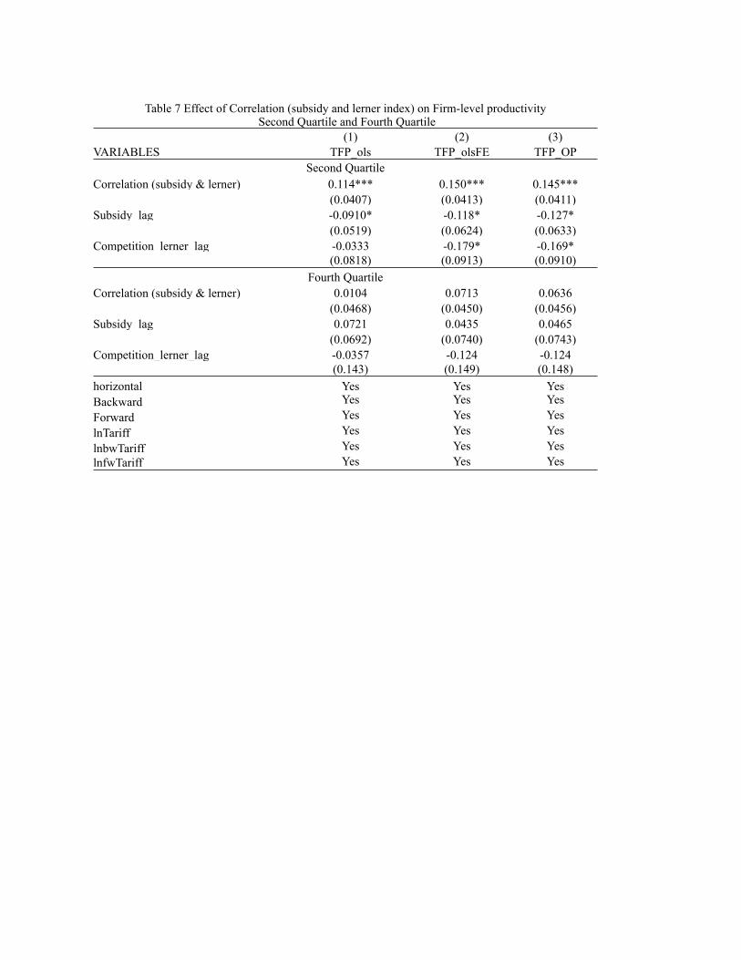
Table 7 Effect of Correlation (subsidy and lerner index) on Firm-level productivity Second Quartile and Fourth Quartile

Table 7 Effect of Correlation (subsidy and lerner index) on Firm-level productivity Second Quartile and Fourth Quartile

Table 7 Effect of Correlation (subsidy and lerner index) on Firm-level productivity Second Quartile and Fourth Quartile

Table 7 Effect of Correlation (subsidy and lerner index) on Firm-level productivity Second Quartile and Fourth Quartile

(1) (2) (3)VARIABLES TFP_ols TFP_olsFE TFP_OP

Second Quartile Second Quartile Second Quartile Second Quartile Correlation (subsidy & lerner) 0.114*** 0.150*** 0.145***

(0.0407) (0.0413) (0.0411)Subsidy_lag -0.0910* -0.118* -0.127*

(0.0519) (0.0624) (0.0633)Competition_lerner_lag -0.0333 -0.179* -0.169*

(0.0818) (0.0913) (0.0910)Fourth QuartileFourth QuartileFourth QuartileFourth Quartile

Correlation (subsidy & lerner) 0.0104 0.0713 0.0636(0.0468) (0.0450) (0.0456)

Subsidy_lag 0.0721 0.0435 0.0465(0.0692) (0.0740) (0.0743)

Competition_lerner_lag -0.0357 -0.124 -0.124(0.143) (0.149) (0.148)

horizontal Yes Yes YesBackward Yes Yes YesForward Yes Yes YeslnTariff Yes Yes YeslnbwTariff Yes Yes YeslnfwTariff Yes Yes Yes

Table 8 Effect of Correlation (subsidy and lerner index) on Aggregate Firm ProductivityTable 8 Effect of Correlation (subsidy and lerner index) on Aggregate Firm ProductivityTable 8 Effect of Correlation (subsidy and lerner index) on Aggregate Firm ProductivityTable 8 Effect of Correlation (subsidy and lerner index) on Aggregate Firm ProductivityDependent: City-Industry Aggregate TFPDependent: City-Industry Aggregate TFPDependent: City-Industry Aggregate TFPDependent: City-Industry Aggregate TFP

OLS OLS with FEs OPcor_subsidy_lerner 0.0348* 0.0796*** 0.0689***

(0.0178) (0.0192) (0.0186)stateshare_aggre 0.00506** 0.0288*** 0.0201***

(0.00243) (0.00530) (0.00422)horizontal -0.0546 -0.0717 -0.0696

(0.266) (0.259) (0.258)backward 3.953*** 3.546*** 3.654***

(0.984) (0.923) (0.923)forward 0.360 0.459 0.434

(0.487) (0.419) (0.432)subsidy_lag -0.0620 -0.0640 -0.125

(0.0894) (0.123) (0.113)lerner_lag -0.233*** -0.355*** -0.347***

(0.0798) (0.0869) (0.0871)lnTariff -0.190*** -0.164*** -0.169***

(0.0412) (0.0394) (0.0392)lnbwTariff -0.155** -0.135* -0.137*

(0.0763) (0.0716) (0.0718)lnfwTariff 0.0450*** 0.0409*** 0.0412***

(0.0154) (0.0150) (0.0147)Constant 1.353** 2.195*** 2.001*** (0.510) (0.457) (0.468)Industry FEs Yes Yes YesCity FEs Yes Yes YesYear Dummies Yes Yes YesObservations 76,923 76,923 76,923R-squared 0.476 0.458 0.467

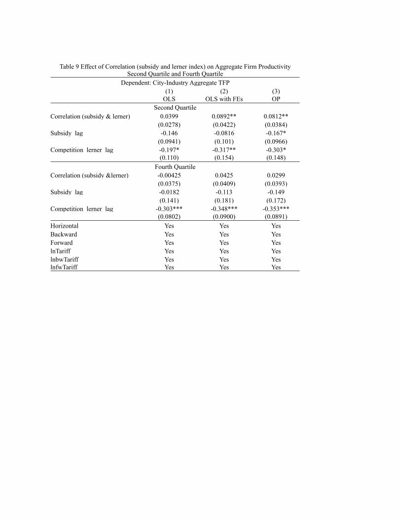
Table 9 Effect of Correlation (subsidy and lerner index) on Aggregate Firm ProductivitySecond Quartile and Fourth Quartile

Table 9 Effect of Correlation (subsidy and lerner index) on Aggregate Firm ProductivitySecond Quartile and Fourth Quartile

Table 9 Effect of Correlation (subsidy and lerner index) on Aggregate Firm ProductivitySecond Quartile and Fourth Quartile

Table 9 Effect of Correlation (subsidy and lerner index) on Aggregate Firm ProductivitySecond Quartile and Fourth Quartile

Dependent: City-Industry Aggregate TFP Dependent: City-Industry Aggregate TFP Dependent: City-Industry Aggregate TFP Dependent: City-Industry Aggregate TFP (1) (2) (3)

OLS OLS with FEs OPSecond QuartileSecond QuartileSecond QuartileSecond Quartile

Correlation (subsidy & lerner) 0.0399 0.0892** 0.0812**(0.0278) (0.0422) (0.0384)

Subsidy_lag -0.146 -0.0816 -0.167*(0.0941) (0.101) (0.0966)

Competition_lerner_lag -0.197* -0.317** -0.303*(0.110) (0.154) (0.148)

Fourth QuartileFourth QuartileFourth QuartileFourth QuartileCorrelation (subsidy &lerner) -0.00425 0.0425 0.0299

(0.0375) (0.0409) (0.0393)Subsidy_lag -0.0182 -0.113 -0.149

(0.141) (0.181) (0.172)Competition_lerner_lag -0.303*** -0.348*** -0.353***

(0.0802) (0.0900) (0.0891)Horizontal Yes Yes YesBackward Yes Yes YesForward Yes Yes YeslnTariff Yes Yes YeslnbwTariff Yes Yes YeslnfwTariff Yes Yes Yes

Table 10 Effect of Correlation (tariff and lerner index) on Firm ProductivityTable 10 Effect of Correlation (tariff and lerner index) on Firm ProductivityTable 10 Effect of Correlation (tariff and lerner index) on Firm ProductivityTable 10 Effect of Correlation (tariff and lerner index) on Firm ProductivityDependent: Firm-level TFPDependent: Firm-level TFPDependent: Firm-level TFPDependent: Firm-level TFP

OLS OLS with FEs OPCorrelation (tariff&lerner) 0.0833*** 0.0722*** 0.0745***

(0.0219) (0.0203) (0.0202)Stateshare -0.00257 -0.00199 -0.00365

(0.00385) (0.00364) (0.00367)Horizontal 0.168* 0.159* 0.161*

(0.0893) (0.0935) (0.0926)Backward 0.688*** 0.698*** 0.692***

(0.255) (0.259) (0.256)Forward 0.123 0.134* 0.131*

(0.0784) (0.0774) (0.0772)Competition_lerner_lag 0.00278 -0.156 -0.144

(0.110) (0.113) (0.113)lnTariff_lag -0.0342** -0.0340** -0.0337**

(0.0144) (0.0139) (0.0141)lnbwTariff_lag -0.0196 -0.0167 -0.0170

(0.0180) (0.0172) (0.0173)lnfwTariff_lag -0.00857*** -0.00806*** -0.00806***

(0.00214) (0.00209) (0.00211)Constant 1.130*** 2.131*** 1.918*** (0.109) (0.112) (0.112)Firm FEs yes yes yesYear Dummies yes yes yesObservations 728,274 728,274 728,274R-squared 0.137 0.179 0.167

Table 11 Effect of Correlation (tariff and lerner index) on Aggregate Firm ProductivityTable 11 Effect of Correlation (tariff and lerner index) on Aggregate Firm ProductivityTable 11 Effect of Correlation (tariff and lerner index) on Aggregate Firm ProductivityTable 11 Effect of Correlation (tariff and lerner index) on Aggregate Firm ProductivityDependent: City-Industry Aggregate TFPDependent: City-Industry Aggregate TFPDependent: City-Industry Aggregate TFPDependent: City-Industry Aggregate TFP

OLS OLS with FEs OPCorrelation (tariff & lerner) 0.0783*** 0.0856*** 0.0873***

(0.0184) (0.0223) (0.0217)Stateshare_aggre 0.00475* 0.0285*** 0.0198***

(0.00243) (0.00522) (0.00415)Horizontal 0.0670 0.0303 0.0355

(0.260) (0.252) (0.251)Backward 3.894*** 3.464*** 3.581***

(1.029) (0.968) (0.967)Forward 0.179 0.304 0.275

(0.521) (0.446) (0.460)Competition_lerner_lag -0.210** -0.339*** -0.329***

(0.0851) (0.0889) (0.0894)lnTariff_lag -0.114*** -0.101*** -0.104***

(0.0271) (0.0264) (0.0260)lnbwTariff_lag -0.0256 -0.0424* -0.0367

(0.0256) (0.0228) (0.0231)lnfwTariff_lag -0.00177 -0.00190 -0.00242

(0.00627) (0.00569) (0.00577)Constant 1.511*** 2.503*** 2.270*** (0.115) (0.119) (0.118)Industry FEs yes yes yesCity FEs yes yse yseYear dummies yes yse yseObservations 76,935 76,935 76,935R-squared 0.472 0.456 0.465

Appendix Table 1 Summary Statistics Appendix Table 1 Summary Statistics Appendix Table 1 Summary Statistics Appendix Table 1 Summary Statistics Appendix Table 1 Summary Statistics Appendix Table 1 Summary Statistics Appendix Table 1 Summary Statistics Appendix Table 1 Summary Statistics LevelsLevelsLevels Growth RatesGrowth RatesGrowth Rates

Obs Mean Std. Dev. Obs Mean Std. Dev.TFP 1,522,730 1.764 0.359 1,072,148 0.055 0.306Stateshare 1,522,730 0.087 0.269 1,072,148 -0.007 0.144Horizontal 1,522,730 0.256 0.142 1,072,148 0.004 0.045Backward 1,522,730 0.078 0.046 1,072,148 0.002 0.015Forward 1,522,730 0.104 0.174 1,072,148 0.004 0.066Ratio_subsidy 1,522,730 0.003 0.019 1,072,148 0.000 0.020Competition_lerner 1,522,730 0.975 0.019 1,072,148 -0.005 0.009Interaction 1,522,730 0.003 0.019 1,072,148 0.000 0.019lnTariff 1,522,730 2.418 0.505 1,072,148 -0.063 0.180lnfwTariff 1,520,636 1.025 1.435 1,070,512 -0.017 0.525lnbwTariff 1,522,730 1.262 0.505 1,072,148 -0.029 0.206Competition_Herf_Subsidy 1,522,730 69.001 80.512 1,072,148 3.726 38.721Subsidy_lag 1,072,148 0.003 0.019 742,902 0.000 0.019Competition_lerner_lag 1,072,148 0.978 0.018 742,902 -0.004 0.008Interaction_lag 1,072,148 0.003 0.019 742,902 0.000 0.019lnTariff_lag 1,072,148 2.446 0.507 742,902 -0.079 0.188lnbwTariff_lag 1,072,148 1.262 0.507 742,902 -0.075 0.175lnfwTariff_lag 1,070,533 1.008 1.471 741,689 -0.342 1.635Cor_tariff_lerner 1,522,730 0.022 0.141 1,072,148 0.016 0.039Cor_subsidy_lerner 1,522,730 0.141 0.083 1,072,148 -0.013 0.057Ratio_newproduct 1,323,089 0.034 0.150 891,800 0.001 0.128Notes: Interation = Ratio_subsidy*Competition_lerner and Interaction_lag = Subsidy_lag * competition_lerner_lag.Notes: Interation = Ratio_subsidy*Competition_lerner and Interaction_lag = Subsidy_lag * competition_lerner_lag.Notes: Interation = Ratio_subsidy*Competition_lerner and Interaction_lag = Subsidy_lag * competition_lerner_lag.Notes: Interation = Ratio_subsidy*Competition_lerner and Interaction_lag = Subsidy_lag * competition_lerner_lag.Notes: Interation = Ratio_subsidy*Competition_lerner and Interaction_lag = Subsidy_lag * competition_lerner_lag.Notes: Interation = Ratio_subsidy*Competition_lerner and Interaction_lag = Subsidy_lag * competition_lerner_lag.Notes: Interation = Ratio_subsidy*Competition_lerner and Interaction_lag = Subsidy_lag * competition_lerner_lag.Notes: Interation = Ratio_subsidy*Competition_lerner and Interaction_lag = Subsidy_lag * competition_lerner_lag.