Industrial Plant Optimization

in Reduced Dimensional

Spaces

Fields Optimization Lecture

Toronto, ON

Giles Laurier

June 4, 2013

Capstone Technology

Agenda

Review of optimization in oil refining

Real Time Optimization

Reduced Space Optimization

Petroleum refining

Refining optimization history

Head office

Refining early adopters (Exxon 1950’s)

Crude selection, operating modes

1961 early SLP paper (Shell oil)

LP not just a fast solution technique Tools to interpret the solution and

run what-if’s.

Refining optimization history

Refineries

Improving process control

Cold

Hot

Advanced Control

1980’s insight that complicated process control problems could be formulated and solved by LP and QP

Refining Optimization Hierarchy

Short Term Plan

Advanced Control

Regulatory Control

Operating Objectives, Component

Prices, Constraints

Operating Targets

Controller Setpoints

Valve Positions

Why Optimize in Real Time?

Short term planning model based on “sustainable” average operation

But things change.....

Crude oil may be different

Processes may be cleaner/more fouled

May be hotter/colder

Real process is nonlinear

Real time optimization intended to capture these opportunities

RTO Approach

Model plant with engineering equations

Heat + mass + hydraulic + equilibrium relationships

Run simulation in parallel to the plant and calibrate to the plant measurements

Optimize the model

Building the simulated plant

Block 2 Block 1

Blocks are solved in the order of material flow

Sequential modular

Sequential modular

Recycles become awkward and need iteration

Block1 Block2 Block3

Block4 Block5

Open Equations

Complete plant model expressed in one large set of (sparse) equations

Run it through a nonlinear root solver

Encouraged by success in solving non linear constraints

Simple still

F zi

V yi

L xi

( 1)0

1 ( 1)

i i

ii

Z K

VK

F

Inputs

Need to fix certain variables to reach solution

Plant instruments have error

Reconciliation

2: ( 100)Min A

2 2 2 2 2

A: W ( 100) W ( 50) W (C 28) W (D 35) W ( 43)

subject to :

0

0

, , , , 0

B C D EMin A B E

A B C D

D E

A B C D E

A: 100

B: 50

C: 28

D: 35 E: 43

Find the smallest set of adjustments to the plant measurements that satisfy the equations

Initial Basis

Offline design software used to fit base case

Results used to provide initial basis for open equations

Thereafter, converged online solutions used as starting basis for next online run

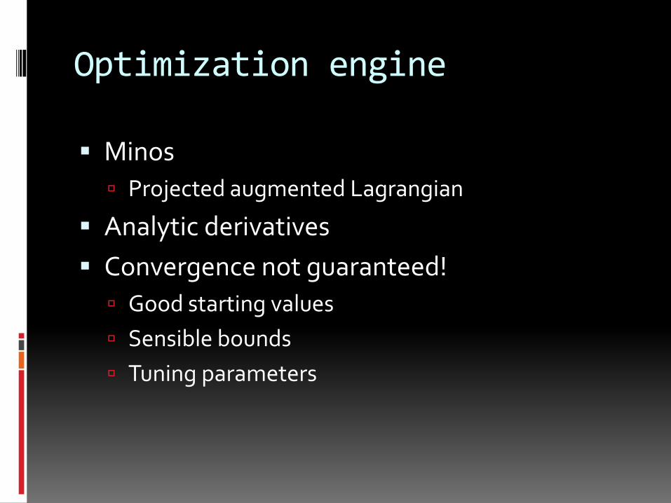
Optimization engine

Minos

Projected augmented Lagrangian

Analytic derivatives

Convergence not guaranteed!

Good starting values

Sensible bounds

Tuning parameters

Gross error detection

Least squares based reconciliation works well when the measurement s are considered to be normally distributed around their true values with approximately known error

Large errors (eg. instrument failures) violate these assumptions and bias reconciliation

RTO systems include pre-screening to eliminate values obviously in error (Wi=0)

Optimization

Fix instrument adjustments and other reconciled performance values

Change objective function Maximize Profit: Products - Feed – Utilities

New setpoints = Old setpoints ± rate limits

RTO Sequence

Check recent history to confirm that plant is steady

Eliminate bad measurements

Fit model to plant data

Calculate new setpoints to increase profit

Check process steady, controls available

Technical challenges

Solving 20+K non linear equations is not fool proof

95% convergence failures occurred during reconciliation phase

Could have put more time trying to make constraints more linear

2 21 2

04.814 4.814

1 2

... T

K KP P

d d

4.8141/i ix dEg: transformations

Catalytic cracker Ultramar QC

~ 27,500 equations

~ 29,500 variables

~ 111,000 derivatives

Reconciliation – 500+ measurements

Optimization 60 setpoints

Execution – 25-40 minutes/cycle

Case study – 40KBPD crude unit

Stream Before (KBPD)

After (KBPD)

Change (KBPD)

LSR 2.47 2.51 0.041

Naphtha 5.15 4.91 -.246

Distillate 4.66 5.03 0.368

VLGO 1.1 1.1 0

LVGO 1.33 1.22 -.103

HVGO 7.68 7.6 -.075

Asphalt 13 13.02 0.018

NET PROFIT

$2220/Day

RTO Benefits

Unit Benefit

Crude units $.01- $.05/BBL

Hydrocracker $.07-$0.3/BBL

FCCU 2% unit profit

Entire refinery $0.50/BBL (Solomon)

Doubts and unease

Was the optimization solution correct?

Stream Before (KBPD)

After (KBPD)

Change (KBPD)

LSR 2.47 2.51 0.041

Naphtha 5.15 4.91 -.246

Distillate 4.66 5.03 0.368

VLGO 1.1 1.1 0

LVGO 1.33 1.22 -.103

HVGO 7.68 7.6 -.075

Asphalt 13 13.02 0.018

NET PROFIT

$2220/Day

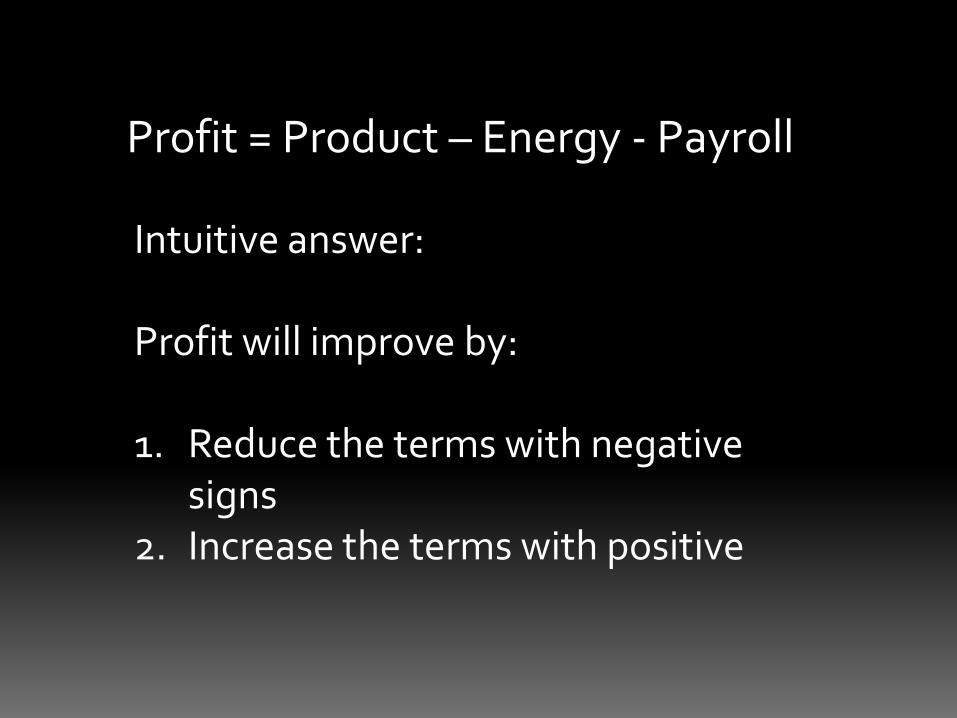
Profit = Product – Energy - Payroll

Intuitive answer: Profit will improve by: 1. Reduce the terms with negative

signs 2. Increase the terms with positive

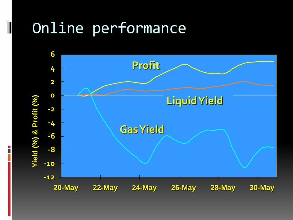
Online performance

-12

-10

-8

-6

-4

-2

0

2

4

6

20-May 22-May 24-May 26-May 28-May 30-May

Gas Yield

Profit

Yie

ld (

%)

& P

rofi

t (%

)

Liquid Yield

Optimization geometry

Constraints

On paper constraints are just a line

In real life – people spend their time avoiding trouble

Constraints can be benign or emotionally charged

In RTO, the operators experienced first hand the simplex method

PROFIT PATH ANALYSIS

7100

7200

7300

7400

7500

7600

7700

7800

7900

8000

8100

510 515 520 525 530

RISER TEMPERATURE

CH

AR

GE

RTO Path

Feed Max Path

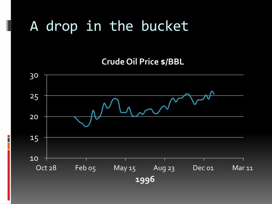
A drop in the bucket

10

15

20

25

30

Oct 28 Feb 05 May 15 Aug 23 Dec 01 Mar 11

1996

Crude Oil Price $/BBL

Behavioural Economics

How emotions and perceptions affect economic decisions

People math ≠ Algebraic math

Risk, reward, gains, losses, time are perceived differently

Daniel Kahneman – Nobel prize economics 2002

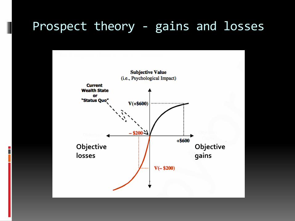
Prospect theory - gains and losses

Objective gains

Objective losses

RTO Path

Feed Max Path

Subjective profit

Objective profit

Familiarity

Comfort is based upon pattern recognition

10,000 hour rule (Gladwell)

Practice makes perfect

Advanced control - imitated the best operator

Value proposition of RTO is to seek out non-obvious benefits

Technology for people

Interact with users

Leverage off patterns

Cruise control

Smart phones

RTO Approach Rethought

How do we model a plant?

Familiar

Modeling the plant

Fundamental design models? Design: What are the best arrangements and sizes of

equipment to maximize ROI

Operating plant Equipment and capability is fixed

Processes must be operated around 70% of design to break even

RTO benefits consistently estimated to be around 3-5%

Can we model a plant just from its historical operating data?

Projection methods (PCA/PLS)

Technique to find patterns in sets of data

Linear algebra (singular value decomposition)

T TX UWV TP

1 0

0 n

w

w

VT

U = X

m×n m×n n×n n×n

VTV = I

UTU = I

Two dimensional example

-3

-2

-1

0

1

2

3

-2 -1.5 -1 -0.5 0 0.5 1 1.5 2 2.5

1st Principal component direction of maximum variation (92%)

2nd Principal component perpendicular to 1st (8%)

Projection Methods

PCA

Find an optimal (least squares) approximation to a matrix X using T1..Tk k<<n

PLS

Find a projection that approximates X well, and correlates with Y

T

T

X TP

Y TC

Happenstance plant data

Number of measurements >> rank (true dimensionality)

Every engineering relationship removes 1 degree of freedom

However operator rules of thumb also remove degrees of freedom

Projection Model

Models the correlation between variables caused by:

Fundamental engineering relationships

Operator preferences

This is not the full space

It is a subspace within which the operator is familiar

Flow example revisited

A

B

C

D E

1 1 1 1 1

2 2 2 2 2

m m m m m

A B C D E

A B C D E

A B C D E

Although we have 5 columns, the rank of the matrix =3 A = B + C + D D = E

Latent space optimization

subject to

X

l Y u

T

( , ) c xT tmaximize F x y d y

2

i

i Ti

TB

s

Boundaries of sphere

PCA model (linear) TX TP

TY TC PLS model (linear)

Key ideas

Model the plant data directly

Operators don’t like surprises

Projection methods implicitly model the the operator

Does it work?

Is this optimal?

Case Study

Chemical company

If we expand our feed system, how much can we produce and still make on specification product

Flowsheet

Dimensions and data

70 operator setpoints and valve positions

22 lab analyses

1 year of operating data (hourly averages)

PCA analysis results

0

0.1

0.2

0.3

0.4

0.5

0.6

0.7

0.8

0.9

1

1 2 3 4 5 6 7 8 9 10 11 12 13 14 15 16 17 18 19 20 21 22 23

Component

X Variance Explained

Conclusions

Although there were 70 setpoints…

The underlying dimensionality of this data was much lower

With a purely linear model

13 components could explain 90% of the variation

23 components could explain > 97% of the variation

Nonlinearity is not significant over the operating range studied

Results

Latent space optimization Plant capable of 10% rate increase while keeping

product qualities within specification

Identified bottlenecks (valves wide open)

Optimum plausible and familiar Restricted to “typical” plant envelope

Effort 2 man weeks

Result Production within 0.2% of predicted

Globally optimal?

Probably not

Better and feasible

Certainly

Final thoughts

Optimization math ≠ human math

Our ability to make sense of high dimensional and complicated situations is limited

Politics is the art of the possible

Bismarck