Embed Size (px)
Citation preview

Introduction Contracts as a barrier to entry Nonlinear pricing and exclusion BO T (qE , qI ) T (qI ) Comparing
Industrial OrganizationNonlinear pricing and exclusion
Laurent Linnemer
CREST (LEI)
2014/15
1 / 41
Introduction Contracts as a barrier to entry Nonlinear pricing and exclusion BO T (qE , qI ) T (qI ) Comparing
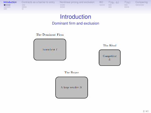
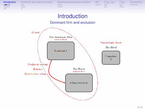
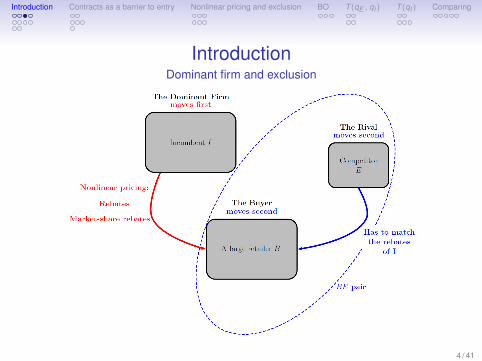
IntroductionDominant firm and exclusion
2 / 41
Introduction Contracts as a barrier to entry Nonlinear pricing and exclusion BO T (qE , qI ) T (qI ) Comparing
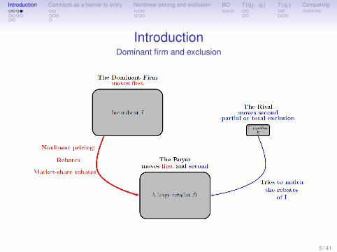
IntroductionDominant firm and exclusion
3 / 41
Introduction Contracts as a barrier to entry Nonlinear pricing and exclusion BO T (qE , qI ) T (qI ) Comparing
IntroductionDominant firm and exclusion
4 / 41
Introduction Contracts as a barrier to entry Nonlinear pricing and exclusion BO T (qE , qI ) T (qI ) Comparing
IntroductionDominant firm and exclusion
5 / 41
Introduction Contracts as a barrier to entry Nonlinear pricing and exclusion BO T (qE , qI ) T (qI ) Comparing
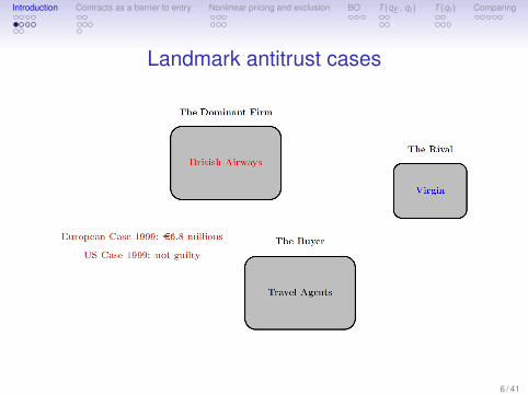
Landmark antitrust cases
6 / 41
Introduction Contracts as a barrier to entry Nonlinear pricing and exclusion BO T (qE , qI ) T (qI ) Comparing
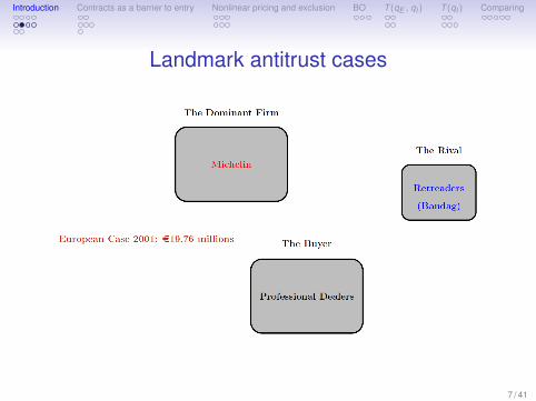
Landmark antitrust cases
7 / 41
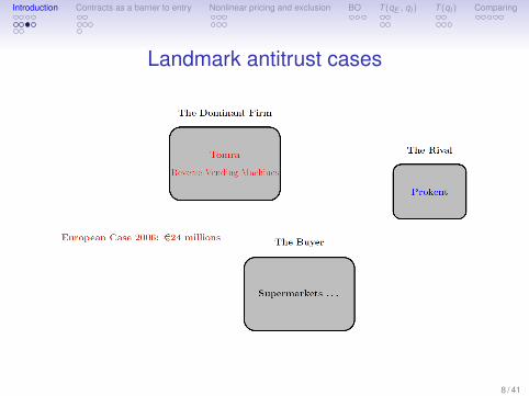
Introduction Contracts as a barrier to entry Nonlinear pricing and exclusion BO T (qE , qI ) T (qI ) Comparing
Landmark antitrust cases
8 / 41
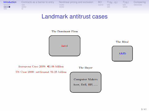
Introduction Contracts as a barrier to entry Nonlinear pricing and exclusion BO T (qE , qI ) T (qI ) Comparing
Landmark antitrust cases
9 / 41
Introduction Contracts as a barrier to entry Nonlinear pricing and exclusion BO T (qE , qI ) T (qI ) Comparing
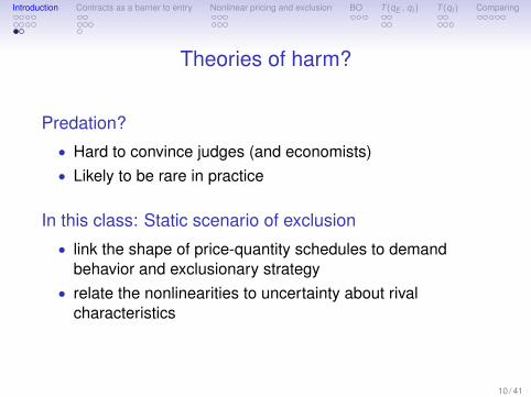
Theories of harm?
Predation?
• Hard to convince judges (and economists)• Likely to be rare in practice
In this class: Static scenario of exclusion
• link the shape of price-quantity schedules to demandbehavior and exclusionary strategy
• relate the nonlinearities to uncertainty about rivalcharacteristics
10 / 41

Introduction Contracts as a barrier to entry Nonlinear pricing and exclusion BO T (qE , qI ) T (qI ) Comparing
Two types of models on exclusion
Naked exclusion (complete information)
• Rasmusen, Ramseyer, and Wiley (1991)• Segal and Whinston (2000)• DeGraba (2013)
Rent shifting (incomplete information)
• Aghion and Bolton (1987)• Marx and Shaffer (1999) (complete info)• Choné and Linnemer (2014a)• Choné and Linnemer (2014b)
11 / 41

Introduction Contracts as a barrier to entry Nonlinear pricing and exclusion BO T (qE , qI ) T (qI ) Comparing
Citations forAghion and Bolton (1987)“Contracts as a barrier to entry” 1987-November 2014: 238 citations
12 / 41
Introduction Contracts as a barrier to entry Nonlinear pricing and exclusion BO T (qE , qI ) T (qI ) Comparing
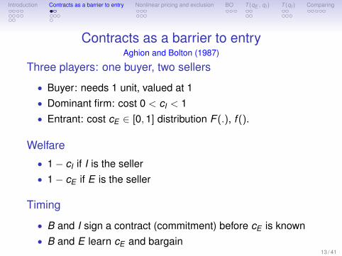
Contracts as a barrier to entryAghion and Bolton (1987)
Three players: one buyer, two sellers
• Buyer: needs 1 unit, valued at 1• Dominant firm: cost 0 < cI < 1• Entrant: cost cE ∈ [0,1] distribution F (.), f ().
Welfare
• 1− cI if I is the seller• 1− cE if E is the seller
Timing
• B and I sign a contract (commitment) before cE is known• B and E learn cE and bargain
13 / 41
Introduction Contracts as a barrier to entry Nonlinear pricing and exclusion BO T (qE , qI ) T (qI ) Comparing
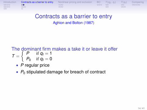
Contracts as a barrier to entryAghion and Bolton (1987)
The dominant firm makes a take it or leave it offerT =
{P if qI = 1P0 if qI = 0
• P regular price• P0 stipulated damage for breach of contract
14 / 41
Introduction Contracts as a barrier to entry Nonlinear pricing and exclusion BO T (qE , qI ) T (qI ) Comparing
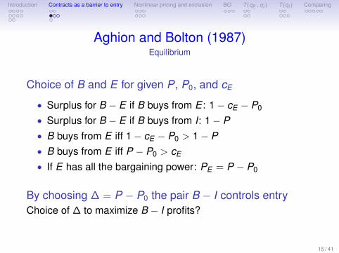
Aghion and Bolton (1987)Equilibrium
Choice of B and E for given P, P0, and cE
• Surplus for B − E if B buys from E : 1− cE − P0
• Surplus for B − E if B buys from I: 1− P• B buys from E iff 1− cE − P0 > 1− P• B buys from E iff P − P0 > cE
• If E has all the bargaining power: PE = P − P0
By choosing ∆ = P − P0 the pair B − I controls entryChoice of ∆ to maximize B − I profits?
15 / 41
Introduction Contracts as a barrier to entry Nonlinear pricing and exclusion BO T (qE , qI ) T (qI ) Comparing
Aghion and Bolton (1987)Equilibrium
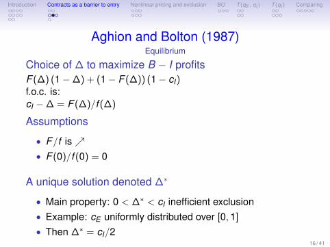
Choice of ∆ to maximize B − I profitsF (∆) (1−∆) + (1− F (∆)) (1− cI)f.o.c. is:cI −∆ = F (∆)/f (∆)
Assumptions
• F/f is↗• F (0)/f (0) = 0
A unique solution denoted ∆∗
• Main property: 0 < ∆∗ < cI inefficient exclusion• Example: cE uniformly distributed over [0,1]
• Then ∆∗ = cI/216 / 41
Introduction Contracts as a barrier to entry Nonlinear pricing and exclusion BO T (qE , qI ) T (qI ) Comparing
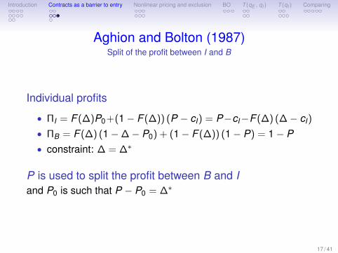
Aghion and Bolton (1987)Split of the profit between I and B
Individual profits
• ΠI = F (∆)P0+(1− F (∆)) (P − cI) = P−cI−F (∆) (∆− cI)
• ΠB = F (∆) (1−∆− P0) + (1− F (∆)) (1− P) = 1− P• constraint: ∆ = ∆∗
P is used to split the profit between B and Iand P0 is such that P − P0 = ∆∗
17 / 41

Introduction Contracts as a barrier to entry Nonlinear pricing and exclusion BO T (qE , qI ) T (qI ) Comparing
DiscussionIn Aghion and Bolton the focus is on the stipulateddamages but
T =
{P if qI = 1 (and qE = 0)P0 if qI = 0 (and qE = 1)
equivalent to
T = P0 + (P − P0)qI
Three interpretations
• stipulated damages• two-part tariff (with price below marginal cost)• exclusivity offer
Also not clear if the price schedule is of the formT (qI) or T (qE ,qI)
18 / 41
Introduction Contracts as a barrier to entry Nonlinear pricing and exclusion BO T (qE , qI ) T (qI ) Comparing
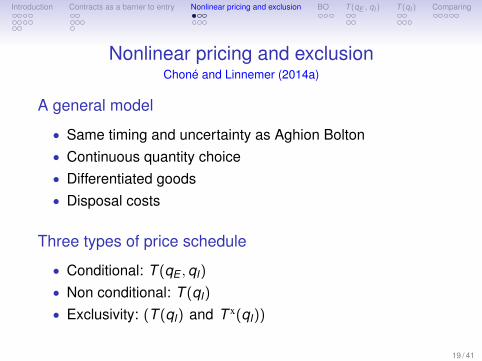
Nonlinear pricing and exclusionChoné and Linnemer (2014a)
A general model
• Same timing and uncertainty as Aghion Bolton• Continuous quantity choice• Differentiated goods• Disposal costs
Three types of price schedule
• Conditional: T (qE ,qI)
• Non conditional: T (qI)
• Exclusivity: (T (qI) and T x(qI))
19 / 41
Introduction Contracts as a barrier to entry Nonlinear pricing and exclusion BO T (qE , qI ) T (qI ) Comparing
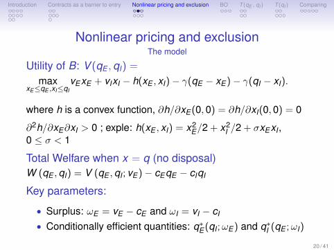
Nonlinear pricing and exclusionThe model
Utility of B: V (qE ,qI) =
maxxE≤qE ,xI≤qI
vExE + vIxI − h(xE , xI)− γ(qE − xE )− γ(qI − xI).
where h is a convex function, ∂h/∂xE (0,0) = ∂h/∂xI(0,0) = 0
∂2h/∂xE∂xI > 0 ; exple: h(xE , xI) = x2E/2 + x2
I /2 + σxExI ,0 ≤ σ < 1
Total Welfare when x = q (no disposal)W (qE ,qI) = V (qE ,qI ; vE )− cEqE − cIqI
Key parameters:
• Surplus: ωE = vE − cE and ωI = vI − cI
• Conditionally efficient quantities: q∗E (qI ;ωE ) and q∗I (qE ;ωI)
20 / 41
Introduction Contracts as a barrier to entry Nonlinear pricing and exclusion BO T (qE , qI ) T (qI ) Comparing
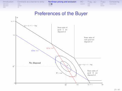
Preferences of the Buyer
W = cst
No disposal
Some units ofgood I are
disposed of
Some units ofeach good are
disposed of
Some units ofgood E are
disposed of
qI = vI + γ − σqE
qE = vE + γ − σqIq∗∗I
q∗∗E
A
vI + γ
vE + γ
qI
qE
q∗I(qE ;ωI)
ωI
q∗E(qI ;ωE)
ωE
21 / 41
Introduction Contracts as a barrier to entry Nonlinear pricing and exclusion BO T (qE , qI ) T (qI ) Comparing
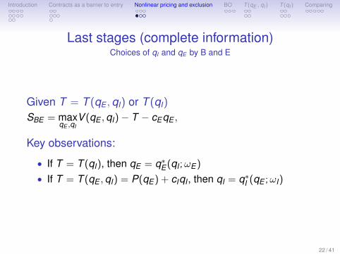
Last stages (complete information)Choices of qI and qE by B and E
Given T = T (qE ,qI) or T (qI)
SBE = maxqE ,qI
V (qE ,qI)− T − cEqE ,
Key observations:
• If T = T (qI), then qE = q∗E (qI ;ωE )
• If T = T (qE ,qI) = P(qE ) + cIqI , then qI = q∗I (qE ;ωI)
22 / 41
Introduction Contracts as a barrier to entry Nonlinear pricing and exclusion BO T (qE , qI ) T (qI ) Comparing
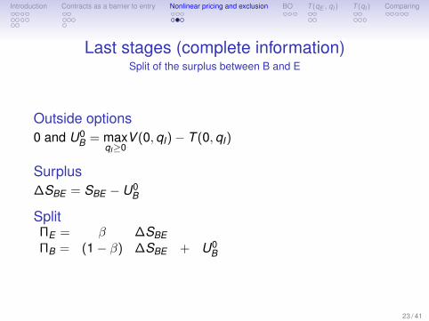
Last stages (complete information)Split of the surplus between B and E
Outside options0 and U0
B = maxqI≥0
V (0,qI)− T (0,qI)
Surplus∆SBE = SBE − U0
B
SplitΠE = β ∆SBEΠB = (1− β) ∆SBE + U0
B
23 / 41
Introduction Contracts as a barrier to entry Nonlinear pricing and exclusion BO T (qE , qI ) T (qI ) Comparing
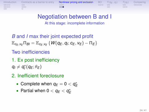
Negotiation between B and IAt this stage: incomplete information
B and I max their joint expected profitEcE ,vE ΠBI = EcE ,vE {W (qE ,qI ; cE , vE )− ΠE}
Two inefficiencies
1. Ex post inefficiencyqI 6= q∗I (qE ; θE )
2. Inefficient foreclosure
• Complete when qE = 0 < q∗E• Partial when 0 < qE < q∗E
24 / 41
Introduction Contracts as a barrier to entry Nonlinear pricing and exclusion BO T (qE , qI ) T (qI ) Comparing
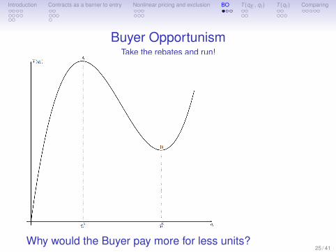
Buyer OpportunismTake the rebates and run!
Why would the Buyer pay more for less units?25 / 41
Introduction Contracts as a barrier to entry Nonlinear pricing and exclusion BO T (qE , qI ) T (qI ) Comparing
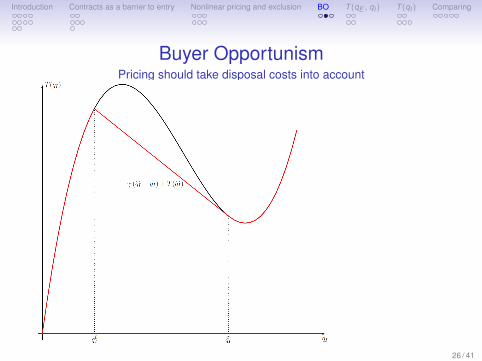
Buyer OpportunismPricing should take disposal costs into account
26 / 41
Introduction Contracts as a barrier to entry Nonlinear pricing and exclusion BO T (qE , qI ) T (qI ) Comparing
Buyer OpportunismOptimality result
PropositionAt the second-best optimum, the buyer consumes all units (ofboth goods) she has purchased.• Good E: BI have nothing to gain from pushing B to
purchase too much• Good I: A matter of credibility⇒ ∂T/∂qI ≥ −γ
27 / 41
Introduction Contracts as a barrier to entry Nonlinear pricing and exclusion BO T (qE , qI ) T (qI ) Comparing
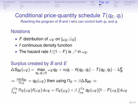
Conditional price-quantity schedule T (qE ,qI)Rewriting the program of B and I who can control both qE and qI
Notations
• F distribution of ωE on [ωE , ωE ]
• f continuous density function• The hazard rate f/(1− F ) is↗ in ωE .
Surplus created by B and E∆SBE (ωE ) = max
qE ,qI≥0ωEqE + vIqI − h(qE ,qI)− T (qE ,qI)− U0
B
⇒ ∂∆SBE∂ωE
= qE (ωE ) then using ΠE = β∆SBE ⇒∫ ωEωE
ΠE (ωE )f (ωE ) dωE = ΠE (ωE ) + β∫ ωEωE
qE (ωE )[1− F (ωE )] dωE
28 / 41
Introduction Contracts as a barrier to entry Nonlinear pricing and exclusion BO T (qE , qI ) T (qI ) Comparing
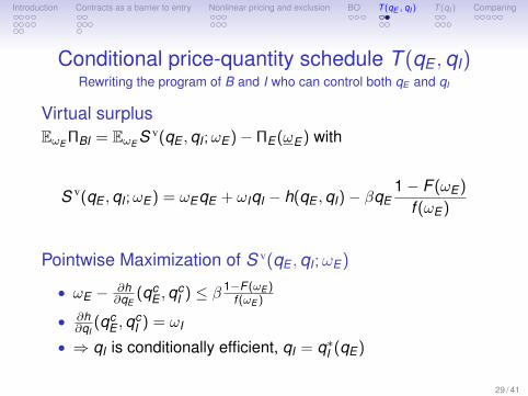
Conditional price-quantity schedule T (qE ,qI)Rewriting the program of B and I who can control both qE and qI
Virtual surplusEωE ΠBI = EωE S v(qE ,qI ;ωE )− ΠE (ωE ) with
S v(qE ,qI ;ωE ) = ωEqE + ωIqI − h(qE ,qI)− βqE1− F (ωE )
f (ωE )
Pointwise Maximization of S v(qE ,qI ;ωE )
• ωE − ∂h∂qE
(qcE ,q
cI ) ≤ β 1−F (ωE )
f (ωE )
• ∂h∂qI
(qcE ,q
cI ) = ωI
• ⇒ qI is conditionally efficient, qI = q∗I (qE )
29 / 41
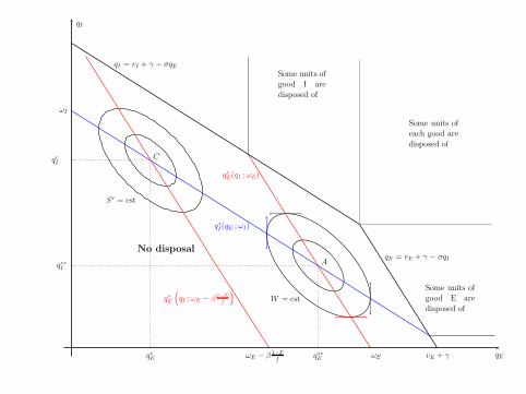
W = cst
qcI
qcE
C
q∗E
(qI ;ωE − β 1−F
f
)
ωE − β 1−Ff
Sv = cst
No disposal
Some units ofgood I are
disposed of
Some units ofeach good are
disposed of
Some units ofgood E are
disposed of
qI = vI + γ − σqE
qE = vE + γ − σqIq∗∗I
q∗∗E
A
vE + γ
qI
qE
q∗I(qE ;ωI)
ωI
q∗E(qI ;ωE)
ωE
Introduction Contracts as a barrier to entry Nonlinear pricing and exclusion BO T (qE , qI ) T (qI ) Comparing
Conditional schedule T (qE ,qI)
Proposition
1. B and I agree on T = P(qE ) + cIqI with P ′′ < 0 and
P ′(qE ) = β(1− F (ωE ))/f (ωE )
2. ∀ωE , qcE ≤ q∗∗E . The quantity purchased from the
incumbent firm, qcI = q∗I (qc
E ;ωE ), is efficient given qcE and
distorted upwards relative to q∗∗I .3. The magnitude of the disposal costs, γ, does not affect the
buyer’s supply policy or the price quantity scheduleT (qE ,qI).
Remark: No market share rebates (suboptimal)
31 / 41
Introduction Contracts as a barrier to entry Nonlinear pricing and exclusion BO T (qE , qI ) T (qI ) Comparing
Unconditional price-quantity schedule T (qI)Rewriting the program of B and I
The key: qE is conditionally efficient
• BI can control qE only through qI
• ⇒ qE = q∗E (qI ;ωE )
Surplus created by B and E∆SBE (ωE ) =maxqI≥0
ωEq∗E (qI ;ωE ) + vIqI − h(q∗E (qI ;ωE ),qI)− T (qI)− U0B
⇒ ∂∆SBE∂ωE
= q∗E (qI ;ωE ) then using ΠE = β∆SBE ⇒∫ ωEωE
ΠE (ωE )f (ωE ) dωE =
ΠE (ωE ) + β∫ ωEωE
q∗E (qI ;ωE )[1− F (ωE )] dωE
32 / 41
Introduction Contracts as a barrier to entry Nonlinear pricing and exclusion BO T (qE , qI ) T (qI ) Comparing
Unconditional schedule T (qI)Rewriting the program of B and I
Virtual surplusS̃ v(qI ;ωE ) = S v(q∗E (qI ;ωE ),qI ;ωE ) =
ωEq∗E (qI ;ωE ) + ωIqI − h(q∗E (qI ;ωE ),qI)− βq∗E (qI ;ωE )1−F (ωE )f (ωE )
Pointwise Maximization of S v(q∗E (qI ;ωE ),qI ;ωE )
Technical requirements for equilibria à la Martimort-Stole 2009• Assumption: quasi-concavity of S̃ v(qI ;ωE ) in qI
• Assumption: ∂2S v/∂qI∂ωE < 0
33 / 41
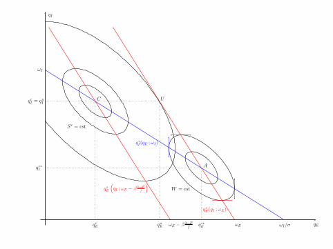
W = cst
ωI/σ
qcI = quI
qcE quE
C U
q∗E
(qI ;ωE − β 1−F
f
)
ωE − β 1−Ff
Sv = cst
q∗∗I
q∗∗E
A
qI
qE
q∗I(qE ;ωI)
ωI
q∗E(qI ;ωE)
ωE
Introduction Contracts as a barrier to entry Nonlinear pricing and exclusion BO T (qE , qI ) T (qI ) Comparing
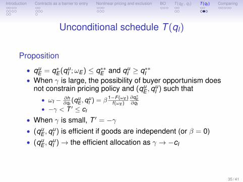
Unconditional schedule T (qI)
Proposition
• quE = q∗E (qu
I ;ωE ) ≤ q∗∗E and quI ≥ q∗∗I
• When γ is large, the possibility of buyer opportunism doesnot constrain pricing policy and (qu
E ,quI ) such that
• ωI − ∂h∂qI
(quE ,q
uI ) = β 1−F (ωE )
f (ωE )∂q∗
E∂qI
• −γ < T ′ ≤ cI
• When γ is small, T ′ = −γ• (qu
E ,quI ) is efficient if goods are independent (or β = 0)
• (quE ,q
uI )→ the efficient allocation as γ → −cI
35 / 41
Introduction Contracts as a barrier to entry Nonlinear pricing and exclusion BO T (qE , qI ) T (qI ) Comparing
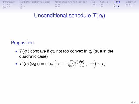
Unconditional schedule T (qI)
Proposition
• T (qI) concave if q∗E not too convex in qI (true in thequadratic case)
• T ′(quI (ωE )) = max
(cI + 1−F (ωE )
f (ωE )
∂q∗E
∂qI, −γ
)< cI
36 / 41
Introduction Contracts as a barrier to entry Nonlinear pricing and exclusion BO T (qE , qI ) T (qI ) Comparing
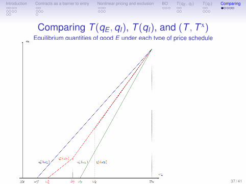
Comparing T (qE ,qI), T (qI), and (T ,T x)Equilibrium quantities of good E under each type of price schedule
37 / 41
Introduction Contracts as a barrier to entry Nonlinear pricing and exclusion BO T (qE , qI ) T (qI ) Comparing
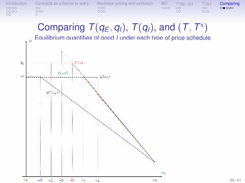
Comparing T (qE ,qI), T (qI), and (T ,T x)Equilibrium quantities of good I under each type of price schedule
38 / 41
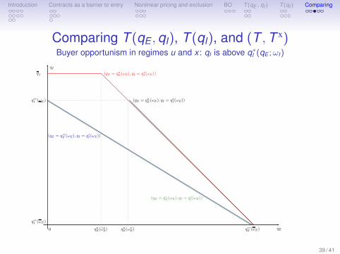
Introduction Contracts as a barrier to entry Nonlinear pricing and exclusion BO T (qE , qI ) T (qI ) Comparing
Comparing T (qE ,qI), T (qI), and (T ,T x)Buyer opportunism in regimes u and x : qI is above q∗
I (qE ;ωI)
0 q∗∗E (ωE)
q∗∗I (ωE)
q∗∗I (ωE)
qI
qI
qE
(qE = q∗∗E (ωE), qI = q∗I(ωE))
(qE = qcE(ωE), qI = qcI(ωE))
(qE = quE(ωE), qI = quI (ωE))
quE(ω̃uE)
(qE = qxE(ωE), qI = qxI (ωE))
quE(ωxE)
39 / 41
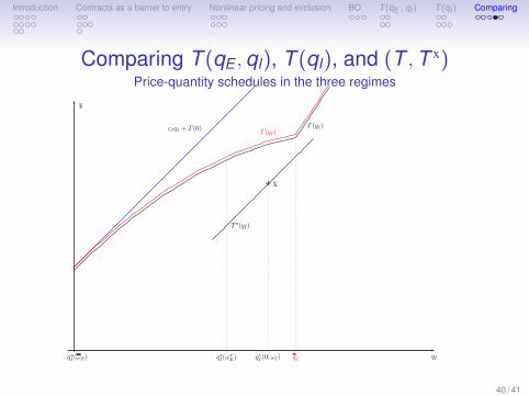
Introduction Contracts as a barrier to entry Nonlinear pricing and exclusion BO T (qE , qI ) T (qI ) Comparing
Comparing T (qE ,qI), T (qI), and (T ,T x)Price-quantity schedules in the three regimes
quI (ωE)
$
qI
cIqI + T (0) T (qI)
qI
T (qI)
+X
T x(qI)
q∗I(0;ωI)qxI (ωxE)
40 / 41
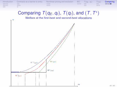
Introduction Contracts as a barrier to entry Nonlinear pricing and exclusion BO T (qE , qI ) T (qI ) Comparing
Comparing T (qE ,qI), T (qI), and (T ,T x)Welfare at the first-best and second-best allocations
41 / 41