Industrial Marketing Management 57 (2016) 127–138

Contents lists available at ScienceDirect

Industrial Marketing Management

Export intensity, scope, and destinations: Evidence from Brazil

Dirk Michael Boehe a,⁎, Gongming Qian b, Mike W. Peng c

a University of Adelaide, Business School, 10 Pulteney Street, Level 10, Office 10.31, Adelaide, SA 5005, Australiab Chinese University of Hong Kong Business School, Department of Management, Room 816, 8/F, Cheng Yu Tung Building, No. 12, Chak Cheung Street, Shatin, N.T., Hong Kongc Jindal School of Management, University of Texas at Dallas, 800 West Campbell Road, SM43, Richardson, TX 75080, USA

⁎ Corresponding author.E-mail addresses: dirk.boehe@adelaide.edu.au (D.M. B

qian@baf.msmail.cuhk.edu.hk (G. Qian), mikepeng@utdal

http://dx.doi.org/10.1016/j.indmarman.2016.01.0060019-8501/© 2016 Elsevier Inc. All rights reserved.

a b s t r a c t

a r t i c l e i n f o

Article history:Received 13 January 2015Received in revised form 29 October 2015Accepted 22 January 2016Available online 4 February 2016

How do the three dimensions of geographic export diversification—namely, (1) export intensity, (2) exportscope, and (3) export destinations—interact in determining firm performance? How does the export intensity–performance relationship change considering export scope and destinations? Drawing on institution-basedand resource-based lenses, we argue that differences between home and destination country institutional envi-ronments are amplified by the scope or variety of export destinations. As firm resources nurtured in the homecountry may not fit an increasing number of different foreign institutional environments, the export intensity–firmperformance relationship turns negative. Conversely, our panel data analysis suggests a positive relationshipbetween export intensity and performancewhen exporters from an emerging economy increase their exports toa limited number of other emerging economies. Thus, our findings extend conventional wisdom on the exportintensity–firm performance relationship and suggest that the international marketing strategy literature needsto simultaneously incorporate three dimensions (including export destinations) into the geographic exportdiversification construct.

© 2016 Elsevier Inc. All rights reserved.

Keywords:Emerging economiesExport intensityExport scopeDeveloped economiesInternational marketing strategyFirm performance

1. Introduction

While most research on geographic diversification deals with multi-nationals (Goerzen & Beamish, 2003; Qian et al., 2010; Rugman &Verbeke, 2004), many firms are active in exporting, but have not be-come multinationals (due to their lack of foreign direct investment[FDI]). Such exporters nevertheless have to confront a crucial butunderexplored attention: How can they manage geographic exportdiversification?

A typical measure for geographic export diversification is export in-tensity, which refers to the ratio of export sales to total sales (Zhao &Zou, 2002). Some research shows a positive relationship between ex-port intensity and firm performance. The reason is twofold: (1) moreproductive, competitive and knowledgeable firms export a higherproportion of sales (Bernard & Jensen, 1999; Ling-Yee, 2004), and(2) exporters that aremore engaged in foreign (compared to domestic)markets learn more and thus become more competitive (Ellis et al.,2011; Salomon & Jin, 2008). However, other studies document a neg-ative relationship. This negative relationship has been explained byreduced export price competitiveness due to widespread country-level drivers such as the home country currency appreciation, risingwages, competition by lower cost countries that lead to lower

oehe),las.edu (M.W. Peng).

margins overseas, among other factors (Gao et al., 2010; Ito, 1997;Lu & Beamish, 2001).

These conflicting claims suggest a gap in our understanding of thedrivers of the relationship between export intensity and firm perfor-mance. We argue that the firm-level dimension, export intensity,needs to be concurrently analyzed within the context of country-leveldimensions that take the form of export scope and export destinations.Export scope refers to the dispersion of activities across foreign coun-tries (Chen & Hsu, 2010; Goerzen & Beamish, 2003), which is alsoknown under the export market concentration versus diversificationdebate. This debate has long proposed that the costs and benefits of ex-port scope are contingent on situational factors. Empirical evidence,however, has so far been inconclusive (Dean et al., 2000; Nath et al.,2010; Piercy, 1981). Export destination countries provide such situa-tional factors.

However, prior research has hardly addressed destinationcountry characteristics (for exceptions, see Cavusgil et al., 2004;Natarajarathinam & Nepal, 2012). Therefore, we address tworesearch questions: (1) How do the three distinct dimensions ofgeographic export diversification—namely, export intensity, exportscope, and export destinations—interact in determining firm perfor-mance? (2) How does the export intensity–performance relationshipchangewhen export scope and destinations are included into analyses?These questions are important because their analysis can help exportmanagers to understand how their export strategies contribute tofirm performance.

128 D.M. Boehe et al. / Industrial Marketing Management 57 (2016) 127–138

Drawing on the institution-based and resource-based theories, ourstudy aspires to make three contributions. First, it integrates the threedimensions of geographic export diversification in a comprehensiveframework and thus sharpens the geographic export diversificationconstruct. While there is widespread literature on each individual di-mension, their combined effects have rarely been addressed. Sheddinglight on this gap in understanding is important given the persistent dis-agreementswith respect to the conceptualization and operationalizationof the geographic diversification construct (Hennart, 2007; Verbeke &Forootan, 2012). Thus, an underexplored opportunity lies in combiningexport intensity with export scope and export destination, which resultsin a three-dimensional geographic export diversification construct. Inwhat follows, we emphasize the novel destination country dimensionof the three-dimensional geographic diversification construct.

Second, we build on prior institution-based work that has suggestedthat the international success or failure of firms is contingent on the in-stitutional conditions of the internationalizing firms' home and destina-tion countries (Cuervo-Cazurra & Genc, 2008; Hoskisson et al., 2013;Meyer & Peng, 2005; Peng, 2012; Wan, 2005). We derive hypothesesthat relate geographic export diversification strategies to firm perfor-mance for EE firms that choose DEs or other EEs as their export destina-tions. By uncovering a significant destination country effect, this studybroadly supports the institution-based view. Thus, the institution-based view extends existing explanations for geographic export diversi-fication (Piercy, 1981; Dean et al., 2000).

By shedding light on the inherent trade-offs between different di-mensions of export diversification, this study extends existing learningby exporting theory that has proposed linear relationships between ex-port intensity and firm performance (Ellis et al., 2011; Ling-Yee, 2004).We argue that this relationship can change contingent on the variety(export scope) and the institutional properties of export destinations.Making progress in the learning by exporting literature thereforerequires incorporating the institution-based and resource-based under-pinnings of the export destination dimension.

2. Institution-based and resource-based theories

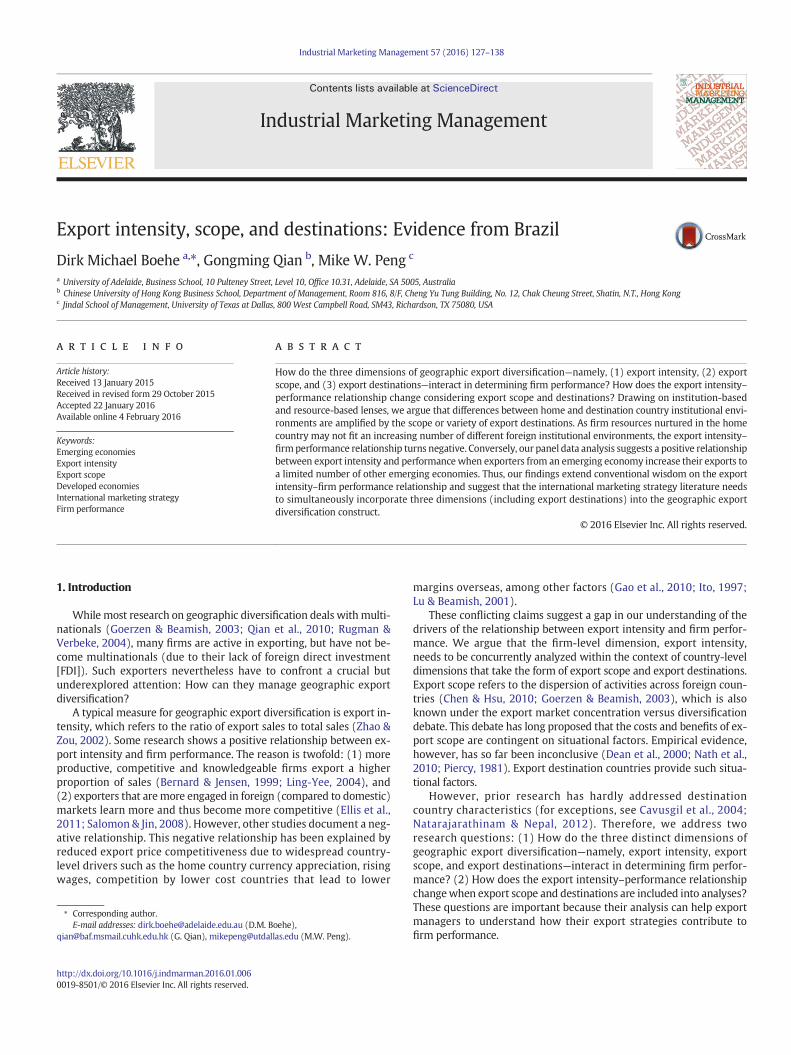
The three dimensions (Fig. 1) represent distinct properties of geo-graphic diversification, i.e. diversification away from the home market(export intensity), across foreign markets (export scope) and acrosseconomically or institutionally dissimilarmarkets (export destinations).The implications of institutional differences between home anddestina-tion countries are the emphasis of this section. The subsequent sectionaddresses how such institutional differences affect firm performancewhen export intensity and scope vary. Our approach builds on theincipient understanding that both export intensity and the exportscope relationships require a contextual explanatory variable—exportdestinations—to properly explain firm performance (Dean et al., 2000;Piercy, 1981; Trofimenko, 2008; Wagner, 2012).

Although some scholars have advocated the use of only one dimen-sion as a geographic diversificationmeasure—foreign sales to total sales(FSTS) for multinationals or export intensity for exporters (Contractor

Fig. 1. The three-dimensional geographic export diversification construct.

et al., 2007; Rugman & Oh, 2011)—the choice of a three dimensionalconstruct is more than a simple measurement issue. Different types ofdestination countries expose exporters to different institutional envi-ronments and consequently to differentmarket challenges towhich ex-porters have to adjust by proficiently deploying their resources andcapabilities.

Prior research has suggested that the home country's institutionalenvironment shapes firm resources and capabilities (Cuervo-Cazurra& Genc, 2008; Ramamurti & Singh, 2009; Wan, 2005), because institu-tions essentially work through incentives that prompt firms to learn, in-novate and thus adapt to competitive challenges (Acemoglu et al., 2005;North, 1990). The resulting resources and capabilities explainwhyfirmsfrom particular EEs perform differently in particular destination coun-tries (Aulakh, Kotabe, & Teegen, 2000; Cuervo-Cazurra et al., 2007;Peng et al., 2008; Hoskisson et al., 2013; Xu & Meyer, 2013). The litera-ture distinguishes betweenweak and strong institutional environments(Peng, 2003; Shinkle & Kriauciunas, 2010). Whereas weak institutionalenvironments imply that competition is impaired, strong ones reflectwell-functioningmarketmechanisms.Weak institutional environmentsat home, often characterized by protectionism, insufficient protection ofintellectual property rights (IPR), oligarchic or monopolistic marketstructures (Acemoglu et al., 2005), are likely to create insufficient incen-tives for firms to develop resources and capabilities to excel in foreignmarkets. For instance, protectionism limits domestic firms' exposureto international competition and thus the incentive to upgrade re-sources and capabilities. Lack of IPR protection limits the opportunitiesfor firms to appropriate the gains of their investments and thus reducesthe propensity to innovate (Khoury & Peng, 2011).

Weaker institutional environments at home may even impose fur-ther burdens on exporters. For example, excessive red tape increasesthe costs of doing business. Likewise, institutional voids, such as thelack of intermediaries that connect buyers and suppliers through infor-mation, product and service flows, tend to raise transaction costs andthus the costs of doing business (Khanna et al., 2005). There is empiricalevidence that firms from EEs that have delayed market-oriented re-forms are less internationalized than firms from EEs that have liberal-ized their economies earlier (Sol & Kogan, 2007).

However, despite such obvious disadvantages of weak institutionalenvironments, some EE firms may develop “adversity advantages”—competitive advantages created by knowing how to work aroundinstitutional voids or by doing business in environments characterizedby infrastructure and resource constraints (Ramamurti & Singh, 2009).In exportmarkets, EE firms need competitive advantages based on valu-able, rare, and difficult-to-imitate resource combinations (Barney, 1991;Kaleka, 2002) to compensate for their liability of foreignness. Adversityadvantages embody context-specific knowledge resources and capabil-ities that can result in competitive advantage in some countries anddisadvantages in others (Cuervo-Cazurra et al., 2007). For instance, EEfirms can address resource and infrastructure constraints in theirhome country and their EE export destinations by developing productsand services for populationswith lower educational, income, and healthlevels or by introducing efficiency innovations and process improve-ments (Jiang et al., 2015; Ramamurti & Singh, 2009).

Finally, larger exporters may use their bargaining power in weak in-stitutional environments to obtainfinancial resources, such as subsidies,tax breaks, and/or cheap loans, from home-country governments(Shinkle & Kriauciunas, 2010; Sun et al., 2015). We argue that these(adversity) advantages and disadvantages that result from EEs' homecountry institutional environments affect exporters' competitivenessdifferently, depending on the characteristics of destination countries(see Table 1). However, the homegrown relationship capability to effec-tively liaise with EE governments—a likely competitive advantage inother EEs—can become a liability in DEs. Thus, the resource-basedview combined with the institution-based view explains why firmsfrom particular countries of origin are differentially competitive inparticular destination countries.

Table 1Exploiting competitive advantages abroad.

Exporters froman emergingeconomy

Export destination countries

Emerging economies Developed economies

Advantages ➢ Adversity advantages➢ Products suited to emerging markets➢ Production and operational excellence

➢ Production and operational excellence

Disadvantages ➢ Higher costs of doing business due to weaker institutions ➢ Higher costs of doing business due to need for adaptations➢ Lack of innovative products➢ Liability of foreignness and emergingness

Economies of scale ➢ Yes, if export intensity is high and few markets are targeted (low export scope) ➢ Very limited

Sources: Based on Cuervo-Cazurra and Genc (2008), Ramamurti and Singh (2009), Wan (2005), and Yamakawa et al. (2013).

129D.M. Boehe et al. / Industrial Marketing Management 57 (2016) 127–138

3. Export intensity, scope, and destination country effects

We treat export intensity as the main effect and consider exportscope and destinations as moderators. This is because export intensityhas been closely associatedwith foreignmarket knowledge, an essentialresource for internationalization (Ellis et al., 2011; Ling-Yee, 2004). No-tably, the controversy around the relationship between export intensityand firm performance constitutes this study's point of departure andlies thus at the heart of our research interest.

The present study takes place in a home country characterized as a“mid-range” EE (Hoskisson et al., 2013) and distinguishes two types ofdestination countries, EEs and DEs. We adopt the perspective of anemerging home economy because international expansion from oneEE into other EEs or DEs is still an embryonic and therefore underrepre-sented phenomenon (Ramamurti & Singh, 2009; Yamakawa et al.,2013; Yamakawa et al., 2008), particularly so for exporting (Leonidouet al., 2010). Consequently, not much is known on the relationship be-tween geographic export diversification strategies and firm perfor-mance of EE firms. Moreover, EE firms are likely to suffer from theliability of emergingness (Madhok & Keyhani, 2012), which exceedsthe typical liability of foreignness discussed in the literature and ex-plains why lessons from DE exporters may not be easily transferred toEE exporters.

If firms from amid-range EE predominantly target other EEs as theirexport destination markets, they may enjoy several advantages overfirms from DEs, such as EE firms' adversity advantages and productssuited to low income populations (Table 1). Limited empirical evidencesuggests that EE firms tend to be more successful in other EEs (Cuervo-Cazurra & Genc, 2008). Equipped with adversity advantages, EE firmsmay achieve higher market shares than competitors (e.g., those fromDEs) without such advantages.

By achieving a higher market share within a particular EE, EE firmsmay bemore likely to economize on scale. Economies of scale can dilutethe up-front sunk costs of exporting and therefore lead to higher effi-ciency. Consequently, raising export intensity and thus economies ofscale in foreign markets may increase firm performance. Moreover,higher export intensity reflects more export market knowledge andhigher commitment to foreign compared to domestic markets, whichmay reduce the liability of foreignness and thus positively affect firmperformance (Ellis et al., 2011; Qian et al., 2013).

However, the potential to achieve economies of scale may be ratherlimited. Specifically, the greater the number of export destinations thefirm targets (high export scope) at a given level of export intensity,the lower the sales volume in each individual country market(Hennart, 2007). Exporters may intentionally do so to reduce risk,build up real options for future expansion, to easily gain small marketshares and due to product specialization (Piercy, 1981). This comes ata cost as different types of institutional and market diversities requirefirms to adapt their marketing mix to specific export destinations, inparticular, cultural diversity (Alden, Hoyer, & Lee, 1993; Lim, Acito, &Rusetski, 2006; Schilke, Reimann, & Thomas, 2009; Sousa & Lengler,2009), administrative diversity (Katsikeas, Samiee, & Theodosiou,

2006; O'Cass & Julian, 2003), and economic diversity (Calantone, Kim,Schmidt, & Cavusgil, 2006). Due to the costs of marketing mix adapta-tions to individual country markets, it is likely that beyond a certainlimit, economies of scale and firm performance may decrease. Themore diverse the requirements to adapt products, the more challengingthe task of coordinating potentially conflicting demands. Such coordina-tion costs are likely to become disproportionate once the number ofexport destination countries becomes too large (Hutzschenreuter &Guenther, 2008).

In addition, diseconomies of scale may arise with increasing exportscope due to increasing logistics costs in EEs. Although EE firms cancount on some adversity advantages that may assist them to copewithweak infrastructure to a certain extent, poor roads, insufficient sea-port or airport capacities, and weak security may lead to losses or dam-ages of merchandise. Thus, at a high level of export scope, performanceis likely to decrease.

Moreover, institutional voids increase transaction costs (Khannaet al., 2005). Transaction costs may be significant particularly incountries passing through institutional transitions, which increaseinformation ambiguity and thus raise the complexity of transactions(Filatotchev et al., 2008). Accordingly, weak institutional environ-ments require firms to emphasize relationship-based exchange in-stead of rule-based exchange. However, establishing trust-basedsocial networks for relationship-based exchange takes more timethan rule-based exchange (Peng, 2003). Hence, once exporterstarget an increasing number of EEs, the additional costs of creatingrelationship-based exchange in so many countries may outweighthe benefits. As a result, by spreading sales in a large number ofEEs, substantially increased costs may offset the competitive advan-tages enjoyed by EE firms.

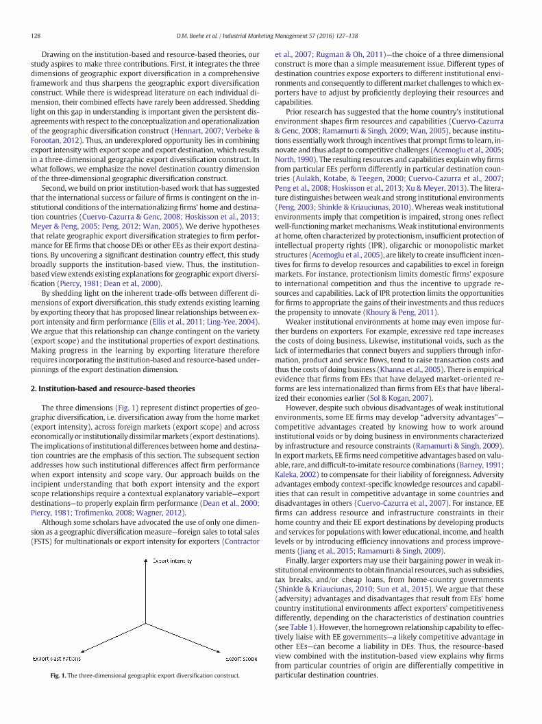
H1a. Export scope moderates the relationship between export intensi-ty and firm performance. For EE firms that predominantly target otherEEs, the relationship between export intensity and firm performancetends to be positive at low levels of export scope.

H1b. Export scope moderates the relationship between export intensi-ty and firm performance. For EE firms that predominantly target otherEEs, the relationship between export intensity and firm performancetends to be negative at high levels of export scope.

The picture is different if EE firms export predominantly to DEswhere the competitive environment is tough given strong institutions,accessible infrastructure, and factor markets (Aulakh et al., 2000; Wan,2005; Yamakawa et al., 2013). EE firms are generally disadvantaged inDEs due to weak institutional environments in their home countries,which result in a lack of innovative products that are competitive withproducts launched by DE firms (Acemoglu et al., 2005). Specifically, EEfirms may not yet comply with the technical standards of DEs (Bartlett& Ghoshal, 2000; Schmitz & Knorringa, 2000). In addition, EEfirms may be disadvantaged as they have insufficient resources and ca-pabilities to overcome the liability of emergingness (Madhok&Keyhani,2012). Therefore, EE firms may have more difficulties in achieving high

130 D.M. Boehe et al. / Industrial Marketing Management 57 (2016) 127–138

market shares than their DE counterparts. Therefore, EE firmsmay forgoeconomies of scale in individual DEs.

To be successful, exporters that target DEs in spite of a more difficultcompetitive environment need to adapt their products, services, andmarketing strategies in order to satisfymore demanding technical, safe-ty, and quality standards (Bartlett & Ghoshal, 2000) and to overcometheir liability of emergingness (Peng, 2012). By successfully adaptingto a DE institutional environment, EE firms signal their legitimacy(Brouthers et al., 2005; Yamakawa et al., 2013). In addition, adaptationhelps EE firms to avoid the loss of their homegrown competitive advan-tages (Cuervo-Cazurra et al., 2007). However, as noted above, adapta-tions come at a significant cost, putting strain on financial performance.

Furthermore, transaction and logistics costs in DEs tend to be lowergiven fewer institutional voids, better transportation infrastructure, andreduced risks of security hazards. Strong institutional environmentsthus make it less costly and more attractive to expand across severalDEs (Yamakawa et al., 2008, 2013). Conversely, easier market accesslikely entails fiercer competition both from DE and also other EEfirms. This also limits the chances for EE firms from mid-range EE toachieve higher market shares and to economize on scale. Therefore,EE firms entering DEs bear the burden of higher unit costs due to for-gone economies of scale and product adaptions, resulting in lowerlevels of firm performance compared to EE firms that predominantlyenter EEs.

H2a. Export scope moderates the relationship between export intensi-ty and firm performance. For EE firms that predominantly target DEs,the positive relationship between export intensity and firm perfor-mance at low levels of export scope is weaker (less positive) than forEE firms that predominantly target other EEs.

H2b. Export scope moderates the relationship between export in-tensity and firm performance. For EE firms that predominantlytarget DEs, the negative relationship between export intensityand firm performance at high levels of export scope is stronger(more negative) than for EE firms that predominantly targetother EEs.

Fig. 2. Hypo

Fig. 2 summarizes our four hypotheses. Fig. 2 organizes the baselineexport intensity–firm performance relationship along two dimensions,low-high export scope on the vertical axis and destination countries,ranging from predominantly emerging to predominantly developedeconomies on the horizontal axis.

4. Methods

4.1. Data

We chose Brazilian exporters because the Latin American region hasbeen considered as under-researched (Aulakh et al., 2000; Cuervo-Cazurra & Dau, 2009; Xu & Meyer, 2013; Vassolo, de Castro, &Gomez-Mejia, 2011). As one of the BRICS nations, Brazil's institutionalcharacteristics allegedly have resulted in high costs of doing business(Fleury & Fleury, 2009) and likely adversity advantages when Brazilianexporters sell abroad. Accordingly, this study uses archival firm-levelexport data from the Brazilian Ministry of Development, Industry, andForeign Trade with information on export volumes per export destina-tion for the period 2001–2010 (inclusive). We also obtained firm-levelaccounting indicators for the largest Brazilian-owned and controlledfirms from the accounting department at the University of SaoPaulo. The final database included an average of more than 160observations per year. With regard to industrial sector breakdown(using 2-digit SIC classification), close to 12% belong to the agricul-tural industry, 15% the food industry, 10% the metal mechanical in-dustry, 8% the chemical industry, 7% the service industry, 5% theelectronics and also 5% the automotive industry.

4.2. Measures

4.2.1. Dependent variablesExport marketing strategy studies have used export performance

(Aulakh et al., 2000) and also firm performance as dependent variables(Ellis et al., 2011). However, export performance and firm performanceare distinct constructs, because firm performance includes domesticmarket performance while export performance does not (Katsikeas

theses.

131D.M. Boehe et al. / Industrial Marketing Management 57 (2016) 127–138

et al., 2000). Moreover, export and domestic market performance seemto be interdependent and jointly affect firm performance (Salomon &Shaver, 2005). Therefore, firm performance provides a more compre-hensive picture of the effects of geographic diversification. Specifically,we used return on sales (ROS) to assess firm performance. The ROSmeasure incorporates returns on export sales and thus has an obviousadvantage over alternative firm performance measures, such as Tobin'sQ (a market value measure) or overall capital efficiency measures, suchas return on assets (ROA). Notwithstanding, we used ROA as a depen-dent variable in robustness tests (regression tables available upon re-quest). These measures were adjusted for industry effects(standardization using industry means and standard deviations) be-cause industry specificity may bias results (Hawawini et al., 2003).

4.2.2. Independent and moderating variablesExport intensity was measured as the ratio of export sales to total

sales. It is a count measure of all export destination countries of a firmper year (Murray et al., 2011).

Export scope is a usefulmeasure as it represents the variety of differ-ent regulatory environments and thus theneed formarketingmix adap-tations, particularly, modifications in products, labelling and packaging.Additional costs in logistics and distribution will also arise when cross-ing national borders. In line with previous research, we include the lin-ear and the quadratic term of export scope (Li, Qian, & Qian, 2015). Thisis because export and international scope have presented curvilinear re-lationships with firm performance in numerous previous studies(Aulakh et al., 2000; Chen & Hsu, 2010; Gomes & Ramaswamy, 1999;Lu & Beamish, 2001; Palich et al., 2000). Both diversification measures(export intensity and export scope)weremean centered tomitigate po-tential multicollinearity concerns when these indicators are interactedwith each other (Aiken & West, 1991).

Given the lack of consensus on the definition of EEs (as opposed toDEs), we used an empirically derived approach based on income levels.To measure the income levels of the export destination countries, weused the logarithm of the export destination country's purchasingpower parity (PPP) adjusted per capita GDP (GDP p.c.). Per capita GDPis strongly correlated with institutional development (Acemoglu et al.,2005), which is central to our argument. We obtained the yearly coun-try data fromunstats.un.org. GDPp.c.wasweighted by the proportion ofeach export target country in the firm's total exports. This compositeindex was used to split the sample by its median in a subsample offirms that export predominantly to DEs (composite index scoresabove US$17,032 per capita GDP at PPP) and to EEs (composite indexscores below US$17,032 per capita GDP at PPP). For instance, whilesome firms may export to both EEs and DEs, a firm that exports 80% ofits sales to DEs and 20% to EEs, fell into the DE group. This approach al-lows for the possibility that firms change groups over time dependingon the composition of its exports.

Our categorization approach is realistic because some EE focused ex-porters may nevertheless target a few importers in DEs as this permitsEE exporters to accompany emergent trends in the developed world,e.g., regarding technical norms, product requirements or internationalmarketing strategies. Thus, even a minor presence in another type ofdestination market can be a form of learning by exporting (Salomon,2006; Ellis et al., 2011). Other firms exporting mainly to EEs may ex-plore future export opportunities in DEswith limited shipments, similarto a real options approach (Chung et al., 2013). Moreover, some ship-ments to EEs of predominantly DE focused exporters may be due to un-solicited orders from EE importers (Liang & Parkhe, 1997).

DEs can include transition economies because emerging economiestend to have a higher GDP at PPP than their nominal GDP whereasDEs tend to have a lower GDP at PPP than their nominal GDP. Whilesome countries may have factor market and institutional characteristicscompatible with either category (see, for instance, Hoskisson et al.,2013, for a detailed analysis of different types of emerging economies),we need to place them into exclusive categories for analytical purposes.

This is in line with previous studies that have adopted similar categori-zation approaches (e.g., Collins, 1990). Nonetheless, our additionalrobustness tests used the log-scaled GDP p.c. composite index as a con-tinuous moderator (see Table 5).

4.2.3. Control variablesIn regard to the firm-specific control variables, we included the loga-

rithm of each exporter's total assets. To avoid potential misspecification,we used the logarithmof total sales for robustness testswith ROA as a de-pendent variable. This value controls for both firm size and scale econo-mies (Hennart, 2007).

Because financial leverage can significantly affect firm performance(Opler & Titman, 1994),we inserted the debt-to-equity ratio as a controlvariable. Exchange rates are essential to understand exporters' perfor-mance (Aulakh et al., 2000).We calculatedfirm-specific bilateral real ef-fective exchange rates for most of the 224 possible export destinations(except for the smaller islands for which the IMF and the World Bankdatabases do not provide data). High exchange rate index values repre-sent disadvantageous conditions for Brazilian exporters.

We also controlled for import intensity because firms may increasetheir imports of intermediate products to raise their competitivenessin times of appreciating home country exchange rates and thusmitigatenegative performance impacts (Abeysinghe & Yeok, 1998).

We introduced additional controls—cultural, administrative, geo-graphic and economic (CAGE) distance—to capture trade costs that en-compass logistics, transaction costs, trade barriers, and other costs.Together, the four types of distance reflect the four dimensions ofGhemawat's (2001) CAGE framework. The indicators used for all fourmeasures were obtained from Berry, Guillen, and Zhou (2010). To con-sider industry-specific characteristics (e.g., certain industries target cer-tain countries to a larger extent than others), we also standardized thefour distance measures by industry.

4.3. Analyses

We used panel regression with firm and period fixed effects (FE) tocontrol for unobserved heterogeneity across thefirms caused by variousfactors, such as exporters' internal resources and differentiated capabil-ities aswell as unobserved temporal shocks (e.g., economic and politicalcrises or other types of external impacts). This adjustment should re-duce the potential endogeneity concerns due to the omission of variablebias and self-selected geographic diversification strategies. TheHausman specification test also suggests fixed effects models due tothe rejection of the Null hypothesis (p b 0.05). We estimate Eq. (1) forthe EE and DE subsamples and Eq. (2) for the entire sample. Conse-quently, Eq. (2) needs to include the composite index of per capitaGDP instead of the GDP-based EE/DE split samples:

ROSit ¼ β0 þ β1Export intensityit þ β2Export scopeitþ β3Export scope squareditþ β4Export intensityit � Export scopeitþ β5Export intensityit � Export scope squareditþ β6GDP p:c: logð Þit þ β7Controlsit þ β13Firm FEþ β14Period FE� Industryþ εit ð1Þ

ROSit ¼ β0 þ β1Export intensityit þ β2Export scopeitþ β3Export scope squaredit

þ β4Export intensityit � Export scopeit þ β5Export intensityit� Export scope squaredit

þ β6GDP p:c: logð Þit � β7GDP p:c: logð Þit � Export intensityitþ β8GDP p:c: logð Þit � Export scopeit þ β9GDP p:c: logð Þit� Export scope squaredit

þ β10GDP p:c: logð Þit � Export intensityit � Export scopeitþ β11GDP p:c: logð Þit � Export intensityit � Export scope squaredit

þ β12Controlsitþ β13Firm FEþ β14Period FE� Industryþ εit

ð2Þ

132 D.M. Boehe et al. / Industrial Marketing Management 57 (2016) 127–138

In Eq. (2), theGDP p.c. composite index represents destination coun-tries' development level. Given our conceptual starting point—therelationship between export intensity and firm performance—we treatexport intensity as our independent variable and export scope aswell as export scope squared as our moderator variables. Thisoperationalization of the interaction effects is in line with Aikenand West (1991), page 68, Fig. 5.2., c.(2). Alternatively, it is, ofcourse, possible to treat export scope asmain effect and export intensityas a moderator. Thus, a study could examine how the curvilinear effectof export scope varies contingent on export intensity and destinations(discussed later, see Section 6.2.).

5. Results

5.1. Descriptive statistics

Tables 2, 3a and 3b present basic statistics. The generally low level ofintercorrelation suggests that multicollinearity is not a significant prob-lem. We also conducted an additional diagnosis using the variance-inflating factor (VIF). The results (the highest value of the VIF is 8.52for the highest order coefficient in the EE economies subsample) wasbelow the common rule of thumb of 10 (Mason & Perreault, 1991),further suggesting little significant problem of multicollinearity.

5.2. Regression results

Table 4 reports regression analyses. The analyses are composed oftwo sets of data, each including four models. The first four models(Models 1–4) are used for EE markets and the last four (Models 5–8)for DEmarkets.Models 1 and 5 are the basicmodels that include all con-trol variables. Models 2 and 6 add the export intensity variable whileModels 3 and 7 introduce both the linear and quadratic export scopevariables. Finally, Models 4 and 8 add the two interaction terms(i.e., one term being the interaction between export intensity and ex-port scope, and the other being the interaction between export intensityand export scope squared). Thus, Models 4 and 8 test H1a and H1b aswell as H2a and H2b for the firms that target EEs and DEs, respectively.

Before testing the hypotheses on the interaction effects of export in-tensity and export scope, we first investigated how and to what degreeexport intensity and export scope individually influence performance.The results on the export intensity variable (in Model 2) is non-significant and highly significant in Model 6 (negative in sign), whichclearly dissent from those of the previous studies (De Loecker, 2007;Gao et al., 2010). The unexpectedly weak or inconsistent relationshipbetween export intensity (the predictor variable) and performance

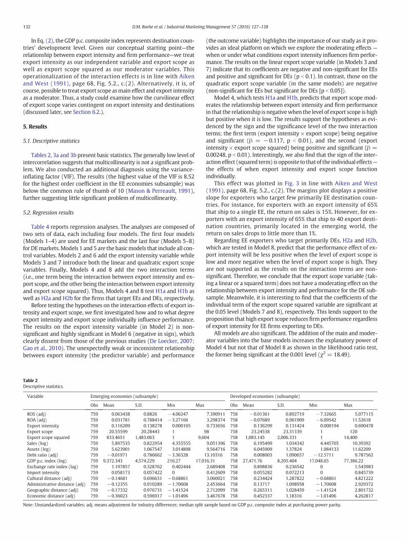
Table 2Descriptive statistics.

Variable Emerging economies (subsample)

Obs Mean S.D. Min Max

ROS (adj) 759 0.063438 0.8826 −4.06247ROA (adj) 759 0.031781 0.788414 −3.27166Export intensity 759 0.116209 0.138278 0.000165Export scope 759 20.55599 20.28443 1Export scope squared 759 833.4651 1,483.063 1 9,6Sales (log) 759 5.897535 0.822954 4.355555Assets (log) 759 5.623901 1.067547 3.014808Debt ratio (adj) 759 −0.01971 0.786662 −3.36328GDP p.c. index (log) 759 9,372.343 4,574.229 216.27 17,0Exchange rate index (lag) 759 1.197857 0.328762 0.402444Import intensity 759 0.058173 0.057422 0Cultural distance (adj) 759 −0.14681 0.696631 −0.68861Administrative distance (adj) 759 −0.12355 0.910289 −1.70608Geographic distance (adj) 759 −0.17332 0.976731 −1.41524Economic distance (adj) 759 −0.36023 0.596917 −1.01496

Note: Unstandardized variables; adj. means adjustment for industry differences; median split

(the outcome variable) highlights the importance of our study as it pro-vides an ideal platform on which we explore the moderating effects —when or under what conditions export intensity influences firm perfor-mance. The results on the linear export scope variable (in Models 3 and7) indicate that its coefficients are negative and non-significant for EEsand positive and significant for DEs (p b 0.1). In contrast, those on thequadratic export scope variable (in the same models) are negative(non-significant for EEs but significant for DEs [p b 0.05]).

Model 4, which tests H1a and H1b, predicts that export scope mod-erates the relationship between export intensity and firm performancein that the relationship is negativewhen the level of export scope is highbut positive when it is low. The results support the hypotheses as evi-denced by the sign and the significance level of the two interactionterms; the first term (export intensity × export scope) being negativeand significant (β = −0.117, p b 0.01), and the second (exportintensity × export scope squared) being positive and significant (β =0.00248, p b 0.01). Interestingly, we also find that the sign of the inter-action effect (squared term) is opposite to that of the individual effects—the effects of when export intensity and export scope functionindividually.

This effect was plotted in Fig. 3 in line with Aiken and West(1991), page 68, Fig. 5.2., c.(2). The margins plot displays a positiveslope for exporters who target few primarily EE destination coun-tries. For instance, for exporters with an export intensity of 65%that ship to a single EE, the return on sales is 15%. However, for ex-porters with an export intensity of 65% that ship to 40 export desti-nation countries, primarily located in the emerging world, thereturn on sales drops to little more than 1%.

Regarding EE exporters who target primarily DEs, H2a and H2b,which are tested in Model 8, predict that the performance effect of ex-port intensity will be less positive when the level of export scope islow and more negative when the level of export scope is high. Theyare not supported as the results on the interaction terms are non-significant. Therefore, we conclude that the export scope variable (tak-ing a linear or a squared term) does not have a moderating effect on therelationship between export intensity and performance for the DE sub-sample. Meanwhile, it is interesting to find that the coefficients of theindividual term of the export scope squared variable are significant atthe 0.05 level (Models 7 and 8), respectively. This lends support to theproposition that high export scope reduces firmperformance regardlessof export intensity for EE firms exporting to DEs.

All models are also significant. The addition of the main andmoder-ator variables into the base models increases the explanatory power ofModel 4 but not that of Model 8 as shown in the likelihood ratio test,the former being significant at the 0.001 level (χ2 = 18.49).

Developed economies (subsample)

Obs Mean S.D. Min Max

7.390911 758 −0.01361 0.892719 −7.32665 5.0771153.298374 758 −0.07689 0.961909 −6.09542 11.526180.733656 758 0.136299 0.131424 0.000194 0.690478

98 758 23.24538 23.31339 1 12004 758 1,083.145 2,006.331 1 14,4009.051396 758 6.195499 1.034342 4.445705 10.393929.564716 758 6.045909 1.37824 1.984133 11.62209

13.10316 758 0.008003 1.090657 −12.5711 9.78756216.31 758 27,471.76 8,205.404 17,048.65 77,386.222.689408 758 0.898836 0.236542 0 1.5439830.412609 758 0.055282 0.072213 0 0.8457393.060021 758 0.234424 1.287822 −0.68861 4.8212222.453664 758 0.13717 1.098958 −1.70608 2.9293722.712099 758 0.265311 1.028459 −1.41524 2.8017323.467678 758 0.452337 1.18316 −1.01496 4.262817

sample based on GDP p.c. composite index at purchasing power parity.

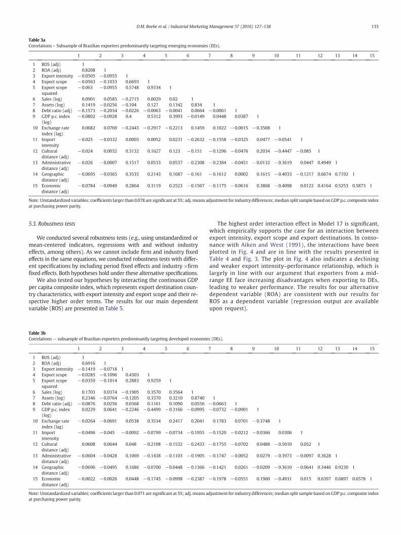
Table 3aCorrelations – Subsample of Brazilian exporters predominantly targeting emerging economies (EEs).

1 2 3 4 5 6 7 8 9 10 11 12 13 14 15

1 ROS (adj) 12 ROA (adj) 0.8208 13 Export intensity −0.0505 −0.0955 14 Export scope −0.0563 −0.1033 0.6693 15 Export scope

squared−0.063 −0.0955 0.5748 0.9334 1

6 Sales (log) 0.0901 0.0585 −0.2715 0.0029 0.02 17 Assets (log) 0.1419 −0.0256 −0.104 0.127 0.1342 0.834 18 Debt ratio (adj) −0.1573 −0.2034 −0.0226 −0.0063 −0.0041 0.0664 −0.0061 19 GDP p.c. index

(log)−0.0802 −0.0928 0.4 0.5312 0.3993 −0.0149 0.0448 0.0387 1

10 Exchange rateindex (lag)

0.0682 0.0769 −0.2443 −0.2917 −0.2213 0.1459 0.1022 −0.0015 −0.3508 1

11 Importintensity

−0.025 −0.0332 0.0003 0.0052 0.0231 −0.2632 −0.1558 −0.0325 0.0477 −0.0541 1

12 Culturaldistance (adj)

−0.024 0.0032 0.3132 0.1627 0.123 −0.151 −0.1296 −0.0476 0.2034 −0.4447 −0.085 1

13 Administrativedistance (adj)

−0.026 −0.0007 0.1517 0.0533 0.0537 −0.2308 −0.2384 −0.0451 −0.0132 −0.3619 0.0447 0.4949 1

14 Geographicdistance (adj)

−0.0695 −0.0365 0.3535 0.2143 0.1687 −0.161 −0.1612 0.0002 0.1615 −0.4033 −0.1217 0.6674 0.7192 1

15 Economicdistance (adj)

−0.0784 −0.0949 0.2864 0.3119 0.2523 −0.1567 −0.1175 −0.0616 0.3868 −0.4098 0.0122 0.4164 0.5253 0.5873 1

Note: Unstandardized variables; coefficients larger than 0.078 are significant at 5%; adj.means adjustment for industry differences;median split sample based onGDP p.c. composite indexat purchasing power parity.

133D.M. Boehe et al. / Industrial Marketing Management 57 (2016) 127–138

5.3. Robustness tests

We conducted several robustness tests (e.g., using unstandardized ormean-centered indicators, regressions with and without industryeffects, among others). As we cannot include firm and industry fixedeffects in the same equations, we conducted robustness tests with differ-ent specifications by including period fixed effects and industry ×firmfixed effects. Both hypotheses hold under these alternative specifications.

We also tested our hypotheses by interacting the continuous GDPper capita composite index, which represents export destination coun-try characteristics, with export intensity and export scope and their re-spective higher order terms. The results for our main dependentvariable (ROS) are presented in Table 5.

Table 3bCorrelations— subsample of Brazilian exporters predominantly targeting developed economie

1 2 3 4 5 6

1 ROS (adj) 12 ROA (adj) 0.6916 13 Export intensity −0.1419 −0.0718 14 Export scope −0.0285 −0.1096 0.4303 15 Export scope

squared−0.0359 −0.1014 0.2883 0.9259 1

6 Sales (log) 0.1703 0.0374 −0.1905 0.3570 0.3564 17 Assets (log) 0.2346 −0.0764 −0.1205 0.3370 0.3210 0.87408 Debt ratio (adj) −0.0876 0.0256 0.0368 0.1161 0.1090 0.05569 GDP p.c. index

(log)0.0229 0.0641 −0.2246 −0.4499 −0.3166 −0.0995

10 Exchange rateindex (lag)

−0.0264 −0.0691 0.0538 0.3534 0.2417 0.2041

11 Importintensity

−0.0496 −0.045 −0.0092 −0.0799 −0.0734 −0.1955

12 Culturaldistance (adj)

0.0608 0.0644 0.048 −0.2108 −0.1532 −0.2433

13 Administrativedistance (adj)

−0.0604 −0.0428 0.1069 −0.1438 −0.1103 −0.1905

14 Geographicdistance (adj)

−0.0696 −0.0495 0.1686 −0.0700 −0.0448 −0.1366

15 Economicdistance (adj)

−0.0022 −0.0026 0.0448 −0.1745 −0.0998 −0.2387

Note: Unstandardized variables; coefficients larger than 0.071 are significant at 5%; adj.means aat purchasing power parity.

The highest order interaction effect in Model 17 is significant,which empirically supports the case for an interaction betweenexport intensity, export scope and export destinations. In conso-nance with Aiken and West (1991), the interactions have beenplotted in Fig. 4 and are in line with the results presented inTable 4 and Fig. 3. The plot in Fig. 4 also indicates a decliningand weaker export intensity–performance relationship, which islargely in line with our argument that exporters from a mid-range EE face increasing disadvantages when exporting to DEs,leading to weaker performance. The results for our alternativedependent variable (ROA) are consistent with our results forROS as a dependent variable (regression output are availableupon request).

s (DEs).

7 8 9 10 11 12 13 14 15

1−0.0663 1−0.0732 −0.0901 1

0.1783 0.0701 −0.3748 1

−0.1520 −0.0212 −0.0366 0.0306 1

−0.1755 −0.0702 0.0488 −0.5010 0.052 1

−0.1747 −0.0052 0.0279 −0.3973 −0.0097 0.3628 1

−0.1421 0.0261 −0.0209 −0.3610 −0.0641 0.3446 0.9230 1

−0.1978 −0.0551 0.1960 −0.4931 0.015 0.6397 0.6897 0.6578 1

djustment for industry differences;median split sample based onGDP p.c. composite index

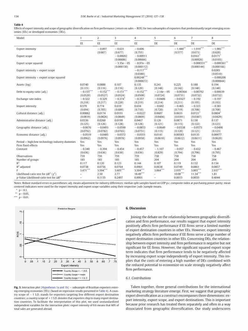
Table 4Effects of export intensity and scope of geographic diversification on firmperformance (return on sales— ROS) for two subsamples of exporters that predominantly target emerging econ-omies (EEs) or developed economies (DEs).

Model 1 2 3 4 5 6 7 8

EE EE EE EE DE DE DE DE

Export intensity −0.897 −0.631 −0.606 −1.480⁎⁎ −1.919⁎⁎⁎ −1.985⁎⁎⁎

(0.687) (0.677) (0.755) (0.577) (0.673) (0.620)Export scope −0.00692 −0.00911 0.0161⁎ 0.0171⁎

(0.00686) (0.00684) (0.00926) (0.0103)Export scope squared −3.35e−05 −8.97e−05 −0.000331⁎⁎ −0.000361⁎⁎

(0.000130) (0.000112) (0.000144) (0.000166)Export intensity × export scope −0.117⁎⁎⁎ 0.0285

(0.0380) (0.0510)Export intensity × export scope squared 0.00248⁎⁎⁎ −0.000206

(0.000672) (0.000844)Assets (log) 0.0740 0.0888 0.107 0.135 0.241 0.225 0.188 0.194

(0.115) (0.116) (0.116) (0.120) (0.148) (0.142) (0.140) (0.140)Debt to equity ratio (adj.) −0.155⁎⁎⁎ −0.152⁎⁎⁎ −0.151⁎⁎⁎ −0.152⁎⁎⁎ −2.14e−05 −0.00364 −0.00792 −0.00639

(0.0520) (0.0527) (0.0524) (0.0508) (0.0724) (0.0731) (0.0732) (0.0732)Exchange rate index −0.322 −0.329 −0.374⁎ −0.357 −0.0406 −0.0327 −0.192 −0.197

(0.218) (0.217) (0.220) (0.219) (0.214) (0.211) (0.195) (0.193)Import intensity 0.579 0.774 0.610 0.634 −0.602 −0.465 −0.321 −0.381

(0.694) (0.705) (0.689) (0.710) (0.720) (0.719) (0.708) (0.708)Cultural distance (adj.) 0.00882 0.0174 0.0191 −0.0227 0.0607 0.0633 0.0721⁎ 0.0804⁎

(0.0819) (0.0826) (0.0849) (0.0809) (0.0404) (0.0391) (0.0387) (0.0429)Administrative distance (adj.) 0.0336 0.0260 0.0199 0.0467 0.126 0.0871 0.130 0.137

(0.125) (0.126) (0.128) (0.128) (0.121) (0.115) (0.122) (0.123)Geographic distance (adj.) −0.0676 −0.0493 −0.0590 −0.0853 −0.0649 −0.0338 −0.0573 −0.0496

(0.0792) (0.0782) (0.0765) (0.0751) (0.115) (0.120) (0.121) (0.123)Economic distance (adj.) −0.0519 −0.0485 −0.0372 −0.0351 0.0141 0.00583 0.0135 0.00977

(0.0962) (0.0976) (0.0978) (0.0958) (0.0610) (0.0612) (0.0611) (0.0620)Period × high/low technology industry dummies Yes Yes Yes Yes Yes Yes Yes YesFirm fixed effects Yes Yes Yes Yes Yes Yes Yes YesConstant −0.340 −0.394 −0.454 −0.457 −1.107 −0.957 −0.432 −0.467

(0.636) (0.636) (0.630) (0.636) (0.829) (0.794) (0.796) (0.795)Observations 759 759 759 759 758 758 758 758Number of groups 185 185 185 185 204 204 204 204R2 0.117 0.120 0.123 0.144 0.107 0.119 0.132 0.134R2 adjusted 0.0738 0.0756 0.0764 0.0961 0.0638 0.0749 0.0861 0.0857F 3.471⁎⁎⁎ 3.594⁎⁎⁎ 3.605⁎⁎⁎ 3.504⁎⁎⁎ 3.064⁎⁎⁎ 2.935⁎⁎⁎ 3.003⁎⁎⁎ 2.937⁎⁎⁎

Likelihood-ratio test for ΔR2 (χ2) – 2.50 2.77 18.49⁎⁎⁎ - 10.08⁎⁎⁎ 11.34⁎⁎⁎ 1.81p-Value Likelihood-ratio test for ΔR2 – 0.1135 0.2497 0.0001 – 0.0015 0.0035 0.4044

Notes: Robust standard errors in parentheses; adj. means adjustment for industry differences; median split samples based on GDP p.c. composite index at purchasing power parity; meancentered indicators were used for the export intensity and export scope variables using their respective (sub-)sample means.⁎ p b 0.1.⁎⁎ p b 0.05.⁎⁎⁎ p b 0.01.

Fig. 3. Interaction plot (Hypotheses 1a and 1b)— subsample of Brazilian exporters enter-ing emerging economies (EEs) (based on regression results presented in Table 4). A coun-try scope of −1 S.D. stands for exporters targeting few different export destinationcountries; a country scope of+1 S.D. denotes that exporters ship tomany export destina-tion countries. To facilitate the interpretation of this plot, we used unstandardizedindependent variables for the interaction plots: export intensity of 0.6 means that 60% oftotal sales are generated abroad.

134 D.M. Boehe et al. / Industrial Marketing Management 57 (2016) 127–138

6. Discussion

Joining the debate on the relationship between geographic diversifi-cation and firm performance, our results suggest that export intensitypositively affects firm performance if EE firms serve a limited numberof export destination countries in other EEs. However, export intensitynegatively affects firm performance if EE firms serve a large number ofexport destination countries in other EEs. Concerning DEs, the relation-ship between export intensity and firm performance is negative but notsignificant for EE firms. However, the significant squared export scopeterm indicates that firm performance tends to be negatively affectedby increasing export scope independently of export intensity. This im-plies that the costs of entering a high number of DEs combined withthe reduced potential to economize on scale strongly negatively affectfirm performance.

6.1. Contributions

Taken together, three general contributions for the internationalmarketing strategy literature emerge. First, we suggest that geographicexport diversification as a construct encompasses three dimensions: ex-port intensity, export scope, and export destinations. This is importantbecause prior research has treated them separately and often in a waydissociated from geographic diversification. Our study underscores

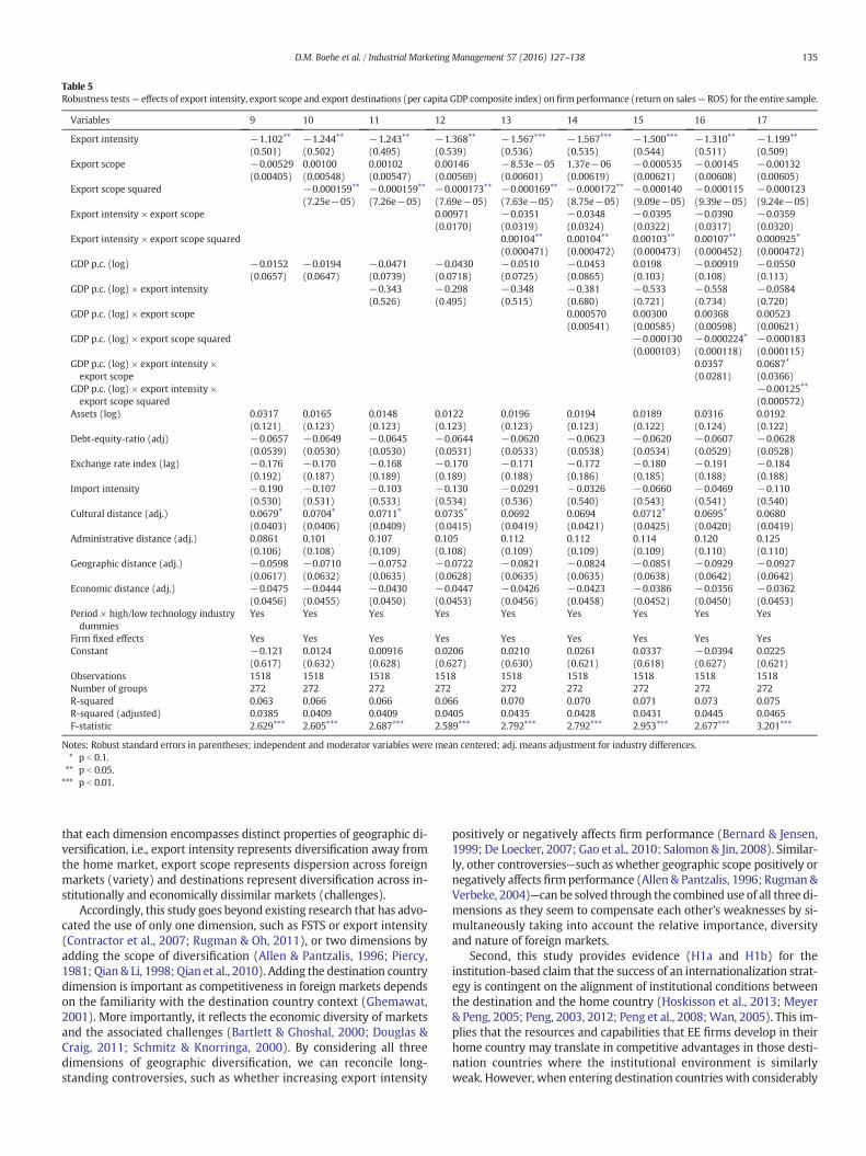
Table 5Robustness tests— effects of export intensity, export scope and export destinations (per capita GDP composite index) on firm performance (return on sales— ROS) for the entire sample.

Variables 9 10 11 12 13 14 15 16 17

Export intensity −1.102⁎⁎ −1.244⁎⁎ −1.243⁎⁎ −1.368⁎⁎ −1.567⁎⁎⁎ −1.567⁎⁎⁎ −1.500⁎⁎⁎ −1.310⁎⁎ −1.199⁎⁎

(0.501) (0.502) (0.495) (0.539) (0.536) (0.535) (0.544) (0.511) (0.509)Export scope −0.00529 0.00100 0.00102 0.00146 −8.53e−05 1.37e−06 −0.000535 −0.00145 −0.00132

(0.00405) (0.00548) (0.00547) (0.00569) (0.00601) (0.00619) (0.00621) (0.00608) (0.00605)Export scope squared −0.000159⁎⁎ −0.000159⁎⁎ −0.000173⁎⁎ −0.000169⁎⁎ −0.000172⁎⁎ −0.000140 −0.000115 −0.000123

(7.25e−05) (7.26e−05) (7.69e−05) (7.63e−05) (8.75e−05) (9.09e−05) (9.39e−05) (9.24e−05)Export intensity × export scope 0.00971 −0.0351 −0.0348 −0.0395 −0.0390 −0.0359

(0.0170) (0.0319) (0.0324) (0.0322) (0.0317) (0.0320)Export intensity × export scope squared 0.00104⁎⁎ 0.00104⁎⁎ 0.00103⁎⁎ 0.00107⁎⁎ 0.000925⁎

(0.000471) (0.000472) (0.000473) (0.000452) (0.000472)GDP p.c. (log) −0.0152 −0.0194 −0.0471 −0.0430 −0.0510 −0.0453 0.0198 −0.00919 −0.0550

(0.0657) (0.0647) (0.0739) (0.0718) (0.0725) (0.0865) (0.103) (0.108) (0.113)GDP p.c. (log) × export intensity −0.343 −0.298 −0.348 −0.381 −0.533 −0.558 −0.0584

(0.526) (0.495) (0.515) (0.680) (0.721) (0.734) (0.720)GDP p.c. (log) × export scope 0.000570 0.00300 0.00368 0.00523

(0.00541) (0.00585) (0.00598) (0.00621)GDP p.c. (log) × export scope squared −0.000130 −0.000224⁎ −0.000183

(0.000103) (0.000118) (0.000115)GDP p.c. (log) × export intensity ×export scope

0.0357 0.0687⁎

(0.0281) (0.0366)GDP p.c. (log) × export intensity ×export scope squared

−0.00125⁎⁎

(0.000572)Assets (log) 0.0317 0.0165 0.0148 0.0122 0.0196 0.0194 0.0189 0.0316 0.0192

(0.121) (0.123) (0.123) (0.123) (0.123) (0.123) (0.122) (0.124) (0.122)Debt-equity-ratio (adj) −0.0657 −0.0649 −0.0645 −0.0644 −0.0620 −0.0623 −0.0620 −0.0607 −0.0628

(0.0539) (0.0530) (0.0530) (0.0531) (0.0533) (0.0538) (0.0534) (0.0529) (0.0528)Exchange rate index (lag) −0.176 −0.170 −0.168 −0.170 −0.171 −0.172 −0.180 −0.191 −0.184

(0.192) (0.187) (0.189) (0.189) (0.188) (0.186) (0.185) (0.188) (0.188)Import intensity −0.190 −0.107 −0.103 −0.130 −0.0291 −0.0326 −0.0660 −0.0469 −0.110

(0.530) (0.531) (0.533) (0.534) (0.536) (0.540) (0.543) (0.541) (0.540)Cultural distance (adj.) 0.0679⁎ 0.0704⁎ 0.0711⁎ 0.0735⁎ 0.0692 0.0694 0.0712⁎ 0.0695⁎ 0.0680

(0.0403) (0.0406) (0.0409) (0.0415) (0.0419) (0.0421) (0.0425) (0.0420) (0.0419)Administrative distance (adj.) 0.0861 0.101 0.107 0.105 0.112 0.112 0.114 0.120 0.125

(0.106) (0.108) (0.109) (0.108) (0.109) (0.109) (0.109) (0.110) (0.110)Geographic distance (adj.) −0.0598 −0.0710 −0.0752 −0.0722 −0.0821 −0.0824 −0.0851 −0.0929 −0.0927

(0.0617) (0.0632) (0.0635) (0.0628) (0.0635) (0.0635) (0.0638) (0.0642) (0.0642)Economic distance (adj.) −0.0475 −0.0444 −0.0430 −0.0447 −0.0426 −0.0423 −0.0386 −0.0356 −0.0362

(0.0456) (0.0455) (0.0450) (0.0453) (0.0456) (0.0458) (0.0452) (0.0450) (0.0453)Period × high/low technology industrydummies

Yes Yes Yes Yes Yes Yes Yes Yes Yes

Firm fixed effects Yes Yes Yes Yes Yes Yes Yes Yes YesConstant −0.121 0.0124 0.00916 0.0206 0.0210 0.0261 0.0337 −0.0394 0.0225

(0.617) (0.632) (0.628) (0.627) (0.630) (0.621) (0.618) (0.627) (0.621)Observations 1518 1518 1518 1518 1518 1518 1518 1518 1518Number of groups 272 272 272 272 272 272 272 272 272R-squared 0.063 0.066 0.066 0.066 0.070 0.070 0.071 0.073 0.075R-squared (adjusted) 0.0385 0.0409 0.0409 0.0405 0.0435 0.0428 0.0431 0.0445 0.0465F-statistic 2.629⁎⁎⁎ 2.605⁎⁎⁎ 2.687⁎⁎⁎ 2.589⁎⁎⁎ 2.792⁎⁎⁎ 2.792⁎⁎⁎ 2.953⁎⁎⁎ 2.677⁎⁎⁎ 3.201⁎⁎⁎

Notes: Robust standard errors in parentheses; independent and moderator variables were mean centered; adj. means adjustment for industry differences.⁎ p b 0.1.⁎⁎ p b 0.05.⁎⁎⁎ p b 0.01.

135D.M. Boehe et al. / Industrial Marketing Management 57 (2016) 127–138

that each dimension encompasses distinct properties of geographic di-versification, i.e., export intensity represents diversification away fromthe home market, export scope represents dispersion across foreignmarkets (variety) and destinations represent diversification across in-stitutionally and economically dissimilar markets (challenges).

Accordingly, this study goes beyond existing research that has advo-cated the use of only one dimension, such as FSTS or export intensity(Contractor et al., 2007; Rugman & Oh, 2011), or two dimensions byadding the scope of diversification (Allen & Pantzalis, 1996; Piercy,1981; Qian & Li, 1998; Qian et al., 2010). Adding the destination countrydimension is important as competitiveness in foreign markets dependson the familiarity with the destination country context (Ghemawat,2001). More importantly, it reflects the economic diversity of marketsand the associated challenges (Bartlett & Ghoshal, 2000; Douglas &Craig, 2011; Schmitz & Knorringa, 2000). By considering all threedimensions of geographic diversification, we can reconcile long-standing controversies, such as whether increasing export intensity

positively or negatively affects firm performance (Bernard & Jensen,1999; De Loecker, 2007; Gao et al., 2010; Salomon & Jin, 2008). Similar-ly, other controversies—such as whether geographic scope positively ornegatively affects firm performance (Allen & Pantzalis, 1996; Rugman &Verbeke, 2004)—can be solved through the combined use of all three di-mensions as they seem to compensate each other's weaknesses by si-multaneously taking into account the relative importance, diversityand nature of foreign markets.

Second, this study provides evidence (H1a and H1b) for theinstitution-based claim that the success of an internationalization strat-egy is contingent on the alignment of institutional conditions betweenthe destination and the home country (Hoskisson et al., 2013; Meyer& Peng, 2005; Peng, 2003, 2012; Peng et al., 2008; Wan, 2005). This im-plies that the resources and capabilities that EE firms develop in theirhome country may translate in competitive advantages in those desti-nation countries where the institutional environment is similarlyweak. However, when entering destination countries with considerably

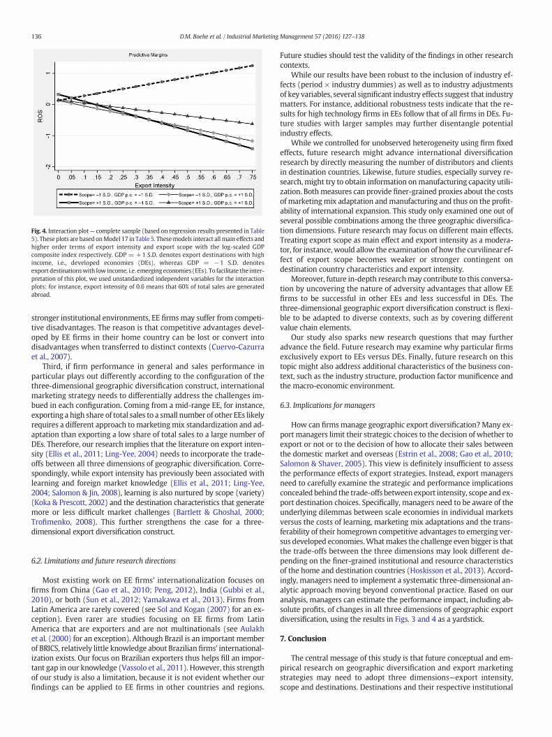
Fig. 4. Interaction plot— complete sample (based on regression results presented in Table5). These plots are based onModel 17 in Table 5. Thesemodels interact all main effects andhigher order terms of export intensity and export scope with the log-scaled GDPcomposite index respectively. GDP = +1 S.D. denotes export destinations with highincome, i.e., developed economies (DEs), whereas GDP = −1 S.D. denotesexport destinationswith low income, i.e. emerging economies (EEs). To facilitate the inter-pretation of this plot, we used unstandardized independent variables for the interactionplots: for instance, export intensity of 0.6 means that 60% of total sales are generatedabroad.

136 D.M. Boehe et al. / Industrial Marketing Management 57 (2016) 127–138

stronger institutional environments, EE firmsmay suffer from competi-tive disadvantages. The reason is that competitive advantages devel-oped by EE firms in their home country can be lost or convert intodisadvantages when transferred to distinct contexts (Cuervo-Cazurraet al., 2007).

Third, if firm performance in general and sales performance inparticular plays out differently according to the configuration of thethree-dimensional geographic diversification construct, internationalmarketing strategy needs to differentially address the challenges im-bued in each configuration. Coming from a mid-range EE, for instance,exporting a high share of total sales to a small number of other EEs likelyrequires a different approach tomarketingmix standardization and ad-aptation than exporting a low share of total sales to a large number ofDEs. Therefore, our research implies that the literature on export inten-sity (Ellis et al., 2011; Ling-Yee, 2004) needs to incorporate the trade-offs between all three dimensions of geographic diversification. Corre-spondingly, while export intensity has previously been associated withlearning and foreign market knowledge (Ellis et al., 2011; Ling-Yee,2004; Salomon & Jin, 2008), learning is also nurtured by scope (variety)(Koka & Prescott, 2002) and the destination characteristics that generatemore or less difficult market challenges (Bartlett & Ghoshal, 2000;Trofimenko, 2008). This further strengthens the case for a three-dimensional export diversification construct.

6.2. Limitations and future research directions

Most existing work on EE firms' internationalization focuses onfirms from China (Gao et al., 2010; Peng, 2012), India (Gubbi et al.,2010), or both (Sun et al., 2012; Yamakawa et al., 2013). Firms fromLatin America are rarely covered (see Sol and Kogan (2007) for an ex-ception). Even rarer are studies focusing on EE firms from LatinAmerica that are exporters and are not multinationals (see Aulakhet al. (2000) for an exception). Although Brazil is an important memberof BRICS, relatively little knowledge about Brazilianfirms' international-ization exists. Our focus on Brazilian exporters thus helps fill an impor-tant gap in our knowledge (Vassolo et al., 2011). However, this strengthof our study is also a limitation, because it is not evident whether ourfindings can be applied to EE firms in other countries and regions.

Future studies should test the validity of the findings in other researchcontexts.

While our results have been robust to the inclusion of industry ef-fects (period × industry dummies) as well as to industry adjustmentsof key variables, several significant industry effects suggest that industrymatters. For instance, additional robustness tests indicate that the re-sults for high technology firms in EEs follow that of all firms in DEs. Fu-ture studies with larger samples may further disentangle potentialindustry effects.

While we controlled for unobserved heterogeneity using firm fixedeffects, future research might advance international diversificationresearch by directly measuring the number of distributors and clientsin destination countries. Likewise, future studies, especially survey re-search,might try to obtain information onmanufacturing capacity utili-zation. Bothmeasures can provide finer-grained proxies about the costsof marketingmix adaptation andmanufacturing and thus on the profit-ability of international expansion. This study only examined one out ofseveral possible combinations among the three geographic diversifica-tion dimensions. Future research may focus on different main effects.Treating export scope as main effect and export intensity as a modera-tor, for instance, would allow the examination of how the curvilinear ef-fect of export scope becomes weaker or stronger contingent ondestination country characteristics and export intensity.

Moreover, future in-depth researchmay contribute to this conversa-tion by uncovering the nature of adversity advantages that allow EEfirms to be successful in other EEs and less successful in DEs. Thethree-dimensional geographic export diversification construct is flexi-ble to be adapted to diverse contexts, such as by covering differentvalue chain elements.

Our study also sparks new research questions that may furtheradvance the field. Future research may examine why particular firmsexclusively export to EEs versus DEs. Finally, future research on thistopic might also address additional characteristics of the business con-text, such as the industry structure, production factor munificence andthe macro-economic environment.

6.3. Implications for managers

How can firmsmanage geographic export diversification?Many ex-port managers limit their strategic choices to the decision of whether toexport or not or to the decision of how to allocate their sales betweenthe domestic market and overseas (Estrin et al., 2008; Gao et al., 2010;Salomon & Shaver, 2005). This view is definitely insufficient to assessthe performance effects of export strategies. Instead, export managersneed to carefully examine the strategic and performance implicationsconcealed behind the trade-offs betweenexport intensity, scope and ex-port destination choices. Specifically, managers need to be aware of theunderlying dilemmas between scale economies in individual marketsversus the costs of learning, marketing mix adaptations and the trans-ferability of their homegrown competitive advantages to emerging ver-sus developed economies.Whatmakes the challenge even bigger is thatthe trade-offs between the three dimensions may look different de-pending on the finer-grained institutional and resource characteristicsof the home and destination countries (Hoskisson et al., 2013). Accord-ingly, managers need to implement a systematic three-dimensional an-alytic approach moving beyond conventional practice. Based on ouranalysis, managers can estimate the performance impact, including ab-solute profits, of changes in all three dimensions of geographic exportdiversification, using the results in Figs. 3 and 4 as a yardstick.

7. Conclusion

The central message of this study is that future conceptual and em-pirical research on geographic diversification and export marketingstrategies may need to adopt three dimensions—export intensity,scope and destinations. Destinations and their respective institutional

137D.M. Boehe et al. / Industrial Marketing Management 57 (2016) 127–138

environments can determine the extent to which homegrown firm re-sources translate into competitive advantages abroad. While researchon the complex interactions among the three dimensions of geographicdiversification is still in its infancy, their further investigation will mostlikely transform and enhance our understanding of the crucial andintriguing relationship between geographic diversification and perfor-mance and its implications for international marketing strategies.

Acknowledgments

We thank Professor Arivaldo dos Santos, University of São Paulo, forproviding accounting data, and we thank Erica Emilia Leite, Aline TiemiFalchetti and Gabriela Brogiolo Da Silva, at Insper São Paulo, for researchassistance.We are grateful to Insper São Paulo and the Jindal Chair at UTDallas for financial assistance.

References

Abeysinghe, T., & Yeok, T. L. (1998). Exchange rate appreciation and export competitive-ness: The case of Singapore. Applied Economics, 30, 51–55.

Acemoglu, D., Johnson, S., & Robinson, J. A. (2005). Institutions as a fundamental cause oflong-run growth. In P. Aghion, & S. Durlauf (Eds.), Handbook of economic growth(pp. 386–472). New York: Elsevier.

Aiken, L. S., & West, S. G. (1991). Multiple regression: Testing and interpreting interactions.London: Sage.

Alden, D. L., Hoyer, W. D., & Lee, C. (1993). Identifying Global and Culture-Specific Dimen-sions of Humor in Advertising: A Multinational Analysis. Journal of Marketing, 57(2),64–75.

Allen, L., & Pantzalis, C. (1996). Valuation of the operating flexibility of multinational cor-porations. Journal of International Business Studies, 27, 633–653.

Aulakh, P. S., Kotabe, M., & Teegen, H. (2000). Export strategies and performance of firmsfrom emerging economies: Evidence from Brazil, Chile, and Mexico. Academy ofManagement Journal, 43, 342–361.

Barney, J. (1991). Firm resources and sustained competitive advantage. Journal ofManagement, 17, 99–120.

Bartlett, C. A., & Ghoshal, S. (2000). Going global: Lessons from late movers. HarvardBusiness Review, 78, 132–142.

Bernard, A. B., & Jensen, J. B. (1999). Exceptional exporter performance: Cause, effect, orboth? Journal of International Economics, 47, 1–25.

Berry, H., Guillen, M. F., & Zhou, N. (2010). An institutional approach to cross-national dis-tance. Journal of International Business Studies, 41, 1460–1480.

Brouthers, L. E., O'Donnell, E., & Hadjimarcou, J. (2005). Generic product strategies foremerging market exports into Triad nation markets: A mimetic isomorphism ap-proach. Journal of Management Studies, 42, 225–245.

Calantone, R. J., Kim, D., Schmidt, J. B., & Cavusgil, S. T. (2006). The influence of internaland external firm factors on international product adaptation strategy and exportperformance: A three-country comparison. Journal of Business Research, 59(2),176–185.

Cavusgil, S. T., Kiyak, T., & Yeniyurt, S. (2004). Complementary approaches to preliminaryforeign market opportunity assessment: Country clustering and country ranking.Industrial Marketing Management, 33(7), 607–617.

Chen, H., & Hsu, C. -W. (2010). Internationalization, resource allocation and firm perfor-mance. Industrial Marketing Management, 39, 1103–1110.

Chung, C. C., Lee, S. -H., Beamish, P. W., Southam, C., & Nam, D. (2013). Pitting real optionstheory against risk diversification theory: International diversification and joint own-ership control in economic crisis. Journal of World Business, 48, 122–136.

Collins, J. M. (1990). A market performance comparison of US firms active in domestic,developed and developing countries. Journal of International Business Studies, 21(2),271–287.

Contractor, F. J., Kumar, V., & Kundu, S. K. (2007). Nature of the relationship between in-ternational expansion and performance: The case of emerging market firms. Journalof World Business, 42, 401–417.

Cuervo-Cazurra, A., & Dau, L. A. (2009). Promarket reforms and firm profitability in devel-oping countries. Academy of Management Journal, 52, 1348–1368.

Cuervo-Cazurra, A., & Genc, M. (2008). Transforming disadvantages into advantages:Developing-country MNEs in the least developed countries. Journal of InternationalBusiness Studies, 39, 957–979.

Cuervo-Cazurra, A., Maloney, M. M., & Manrakhan, S. (2007). Causes of the difficulties ininternationalization. Journal of International Business Studies, 38, 709–725.

De Loecker, J. (2007). Do exports generate higher productivity? Evidence from Slovenia.Journal of International Economics, 73, 69–98.

Dean, D. L., Mengüç, B., & Myers, C. P. (2000). Revisiting firm characteristics, strategy, andexport performance relationship: A survey of the literature and an investigation ofNew Zealand small manufacturing firms. Industrial Marketing Management, 29(5),461–477.

Douglas, S. P., & Craig, C. (2011). Convergence and divergence: Developing a semiglobalmarketing strategy. Journal of International Marketing, 19(1), 82–101.

Ellis, P. D., Davies, H., & Wong, A. H. -K. (2011). Export intensity and marketing in transi-tion economies: Evidence from China. Industrial Marketing Management, 40(4),593–602.

Estrin, S., Meyer, K. E., Wright, M., & Foliano, F. (2008). Export propensity and intensity ofsubsidiaries in emerging economies. International Business Review, 17, 574–586.

Filatotchev, I., Stephan, J., & Jindra, B. (2008). Ownership structure, strategic controls andexport intensity of foreign-invested firms in transition economies. Journal ofInternational Business Studies, 39, 1133–1148.

Fleury, A., & Fleury, M. T. L. (2009). Brazilian multinationals: Surfing the waves of interna-tionalization. In R. Ramamurti, & J. V. Singh (Eds.), Emerging multinationals fromemerging markets (pp. 200–243). Cambridge: Cambridge University Press.

Gao, G. Y., Murray, J. Y., Kotabe, M., & Lu, J. (2010). A strategy tripod perspective on exportbehaviors: Evidence from domestic and foreign firms based in an emerging economy.Journal of International Business Studies, 41, 377–396.

Ghemawat, P. (2001). Distance still matters. The hard reality of global expansion. HarvardBusiness Review, 79, 137–147.

Goerzen, A., & Beamish, P. W. (2003). Geographic scope and multinational enterprise per-formance. Strategic Management Journal, 24, 1289–1306.

Gomes, L., & Ramaswamy, K. (1999). An empirical examination of the form of the rela-tionship between multinationality and performance. Journal of InternationalBusiness Studies, 30(1), 173–187.

Gubbi, S. R., Aulakh, P. S., Ray, S., Sarkar, M. B., & Chitoor, R. (2010). Do international ac-quisitions by emerging-economy firms create shareholder value? The case of Indianfirms. Journal of International Business Studies, 41, 397–418.

Hawawini, G., Subramanian, V., & Verdin, P. (2003). Is performance driven by industry-orfirm-specific factors? A new look at the evidence. Strategic Management Journal, 24,1–16.

Hennart, J. -F. (2007). The theoretical rationale for a multinationality–performance rela-tionship. Management International Review, 47, 423–452.

Hoskisson, R. E., Wright, M., Filatotchev, I., & Peng, M.W. (2013). Emergingmultinationalsfrom mid-range economies: The influence of institutions and factor markets. Journalof Management Studies, 50, 1295–1321.

Hutzschenreuter, T., & Guenther, F. (2008). Performance effects of firms' expansion pathswithin and across industries and nations. Strategic Organization, 6, 47–81.

Ito, K. (1997). Domestic competitive position and export strategy of Japanesemanufactur-ing firms: 1971–1985. Management Science, 43(5), 610–622.

Jiang, Y., Peng,M.W., Yang, X., &Mutlu, C. (2015). Privatization, governance, and survival:MNE investments in private participation projects in emerging economies. Journal ofWorld Business, 50, 294–301.

Kaleka, A. (2002). Resources and capabilities driving competitive advantage in exportmarkets: Guidelines for industrial exporters. Industrial Marketing Management, 31,273–283.

Katsikeas, C. S., Leonidou, L. C., & Morgan, N. A. (2000). Firm-level export performance as-sessment: Review, evaluation and development. Journal of the Academy of MarketingScience, 28(4), 493–511.

Katsikeas, C. S., Samiee, S., & Theodosiou, M. (2006). Strategy fit and performance conse-quences of international marketing standardization. Strategic Management Journal,27(9), 867–890.

Khanna, T., Palepu, K., & Sinha, J. (2005). Strategies that fit emerging markets. HarvardBusiness Review, 83, 63–76.

Khoury, T. A., & Peng, M. W. (2011). Does institutional reform of intellectual propertyrights lead to more inbound FDI? Evidence from Latin America and the Caribbean.Journal of World Business, 46, 337–345.

Koka, B. R., & Prescott, J. E. (2002). Strategic alliances as social capital: A multidimensionalview. Strategic Management Journal, 23(9), 795–816.

Leonidou, L., Katsikeas, C., & Coudounaris, D. (2010). Five decades of business research intoexporting: A bibliographic analysis. Journal of International Management, 16(1),78–91.

Li, L., Qian, G., & Qian, Z. (2015). Should small, young technology-based firms internalizetransactions in their internationalization? Entrepreneurship: Theory and Practice,39(4), 839–862.

Liang, N., & Parkhe, A. (1997). Importer behavior: The neglected counterpart of interna-tional exchange. Journal of International Business Studies, 28(3), 495–530.

Lim, L. K. S., Acito, F., & Rusetski, A. (2006). Development of Archetypes of InternationalMarketing Strategy. Journal of International Business Studies, 37(4), 499–524.

Ling-Yee, L. (2004). An examination of the foreign market knowledge of exporting firmsbased in the People's Republic of China: Its determinants and effect on export inten-sity. Industrial Marketing Management, 33(7), 561–572.

Lu, J. W., & Beamish, P. W. (2001). The internationalization and performance of SMEs.Strategic Management Journal, 22(6/7), 565–586.

Madhok, A., & Keyhani, M. (2012). Acquisitions as entrepreneurship: Asymmetries, op-portunities, and the internationalization of multinationals from emerging economies.Global Strategy Journal, 2, 26–40.

Mason, C. H., & Perreault, W. D., Jr. (1991). Collinearity, power, and interpretation of mul-tiple regression analysis. Journal of Marketing Research, 28, 268–280.

Meyer, K. E., & Peng, M.W. (2005). Probing theoretically into Central and Eastern Europe:Transactions, resources, and institutions. Journal of International Business Studies, 36,600–621.

Murray, J. Y., Gao, G. Y., & Kotabe, M. (2011). Market orientation and performance of ex-port ventures: The process through marketing capabilities and competitive advan-tages. Journal of the Academy of Marketing Science, 39(2), 252–269.

Natarajarathinam, M., & Nepal, B. (2012). A holistic approach to market assessment for amanufacturing company in an emerging economy. Industrial Marketing Management,41(7), 1142–1151.

Nath, P., Nachiappan, S., & Ramanathan, R. (2010). The impact of marketing capability, op-erations capability and diversification strategy on performance: A resource-basedview. Industrial Marketing Management, 39(2), 317–329.

North, D. (1990). Institutions, institutional change, and economic performance. Cambridge:Cambridge University Press.

138 D.M. Boehe et al. / Industrial Marketing Management 57 (2016) 127–138

O'Cass, A., & Julian, C. (2003). Examining firm and environmental influences on exportmarketing mix strategy and export performance of Australian exporters. EuropeanJournal of Marketing, 37(3/4), 366–384.

Opler, T. C., & Titman, S. (1994). Financial distress and corporate performance. Journal ofFinance, 49, 1015–1040.

Palich, L. E., Cardinal, L. B., & Miller, C. C. (2000). Curvilinearity in the diversification-performance linkage: An examination of over three decades of research. StrategicManagement Journal, 21, 155–174.

Peng, M. W. (2003). Institutional transitions and strategic choices. Academy ofManagement Review, 28, 275–296.

Peng, M. W. (2012). The global strategy of emerging multinationals from China. GlobalStrategy Journal, 2, 97–107.

Peng, M. W., Wang, D. Y. L., & Jiang, Y. (2008). An institution-based view of internationalbusiness strategy: A focus on emerging economies. Journal of International BusinessStudies, 39, 920–936.

Piercy, N. (1981). British export market selection and pricing. Industrial MarketingManagement, 10(4), 287–297.

Qian, G., & Li, J. (1998). Multinationality, global market diversification, and risk perfor-mance for the largest U.S. firms. Journal of International Management, 4, 149–170.

Qian, G., Khoury, T. A., Peng, M. W., & Qian, Z. (2010). The performance implications ofintra- and inter-regional geographic diversification. Strategic Management Journal,31, 1018–1030.

Qian, G., Li, L., & Rugman, A. M. (2013). Liability of country foreignness and liability of re-gional foreignness: Their effects on geographic diversification and firm performance.Journal of International Business Studies, 44, 635–647.

Ramamurti, R., & Singh, J. V. (2009). Emerging multinationals from emerging markets. Cam-bridge: Cambridge University Press.

Rugman, A. M., & Oh, C. H. (2011). Methodological issues in the measurement ofmultinationality of US firms. Multinational Business Review, 19, 202–212.

Rugman, A. M., & Verbeke, A. (2004). A perspective on regional and global strategies ofmultinational enterprises. Journal of International Business Studies, 35, 3–18.

Salomon, R. (2006). Learning from exporting: New insights, new perspectives. Cheltenham:Edward Elgar.

Salomon, R., & Jin, B. (2008). Does knowledge spill to leaders or laggards? Exploring in-dustry heterogeneity in learning by exporting. Journal of International BusinessStudies, 39, 132–150.

Salomon, R., & Shaver, J. M. (2005). Export and domestic sales: Their interrelationship anddeterminants. Strategic Management Journal, 26, 855–871.

Schilke, O., Reimann,M., & Thomas, J. S. (2009).WhenDoes International Marketing Stan-dardization Matter to Firm Performance? Journal of International Marketing, 17(4),24–46.

Schmitz, H., & Knorringa, P. (2000). Learning from global buyers. Journal of DevelopmentStudies, 37(2), 177–205.

Shinkle, G. A., & Kriauciunas, A. P. (2010). Institutions, size and age in transition econo-mies: Implications for export growth. Journal of International Business Studies, 41,267–286.

Sol, P. D., & Kogan, J. (2007). Regional competitive advantage based on pioneering eco-nomic reforms: The case of Chilean FDI. Journal of International Business Studies, 38,901–927.

Sousa, C. M. P., & Lengler, J. (2009). Psychic distance, marketing strategy and performancein export ventures of Brazilian firms. Journal of Marketing Management, 25(5-6),591–610.

Sun, S. L., Peng, M. W., Ren, B., & Yan, D. (2012). A comparative ownership advantageframework for cross-border M&As: The rise of Chinese and Indian MNEs. Journal ofWorld Business, 47, 4–16.

Sun, S. L., Peng, M. W., Lee, R. P., & Tan, W. (2015). Institutional open access at home andoutward internationalization. Journal of World Business, 50, 234–246.

Trofimenko, N. (2008). Learning by exporting: Does it matter where one learns? Evidencefrom Colombian manufacturing firms. Economic Development and Cultural Change,56(4), 871–894.

Vassolo, R. S., de Castro, J. O., & Gomez-Mejia, L. R. (2011). Managing in Latin American:Common issues and a research agenda. Academy of Management Perspectives, 25(4),22–36.

Verbeke, A., & Forootan, M. Z. (2012). How good aremultinationality–performance (m–p)empirical studies? Global Strategy Journal, 2, 332–344.

Wagner, J. (2012). International trade and firm performance: A survey of empirical stud-ies since 2006. Review of World Economics, 148(2), 235–267.

Wan, W. P. (2005). Country resource environments, firm capabilities, and corporate di-versification strategies. Journal of Management Studies, 42, 161–182.

Xu, D., & Meyer, K. E. (2013). Linking theory and context: ‘Strategy research in emergingeconomies’ after Wright et al. (2005). Journal of Management Studies, 50, 1322–1346.

Yamakawa, Y., Peng, M.W., & Deeds, D. (2008). What drives new ventures to internation-alize from emerging to developed economies? Entrepreneurship: Theory and Practice,32, 59–82.

Yamakawa, Y., Khavul, S., Peng, M. W., & Deeds, D. (2013). Venturing from emergingeconomies. Strategic Entrepreneurship Journal, 7, 181–196.

Zhao, H., & Zou, S. (2002). The impact of industry concentration and firm location on ex-port propensity and intensity: An empirical analysis of Chinese manufacturing firms.Journal of International Marketing, 10(1), 52–71.