Industrial Applications of Industrial Applications of Response Surface MethodolgyResponse Surface Methodolgy

John BorkowskiJohn BorkowskiMontana State UniversityMontana State University

Pattaya Conference on StatisticsPattaya Conference on StatisticsPattaya, ThailandPattaya, Thailand

Outline of the PresentationOutline of the Presentation

1. The Experimentation Process

2. Screening Experiments

3. 2k Factorial Experiments

4. Optimization Experiments

5. Mixture Experiments

6. Final Comments

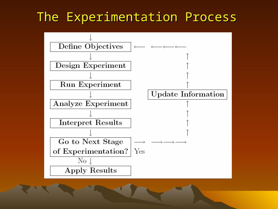
The Experimentation ProcessThe Experimentation Process

Defining Experimental ObjectivesDefining Experimental Objectives

Researchers often discover after running an experiment that the data are insufficient to meet objectives

The first and most important step in an experimental strategy is to clearly state the objectives of the experiment.

The objective is a precise answer to the question “What do you want to know when the experiment is complete?”

2. Screening Experiments2. Screening Experiments

The experimenter wants to determine which process variables are important from a list of potentially important variables.

Screening experiments are economical because a large number of factors can be studied in a small number of experimental runs.

The factors that are found to be important will be used in future experiments. That is, we have screened out the important factors from the list.

2. Screening Experiments2. Screening Experiments

Common screening experiments are 1. Plackett-Burman designs2. Two-level full-factorial (2k) designs 3. Two-level fractional-factorial (2k-p) designs

Plackett-Burman designs allow you to study as many as k-1 factors in k points where k = 12, 20, 24… (k is a multiple of 4 but not a power of 2)

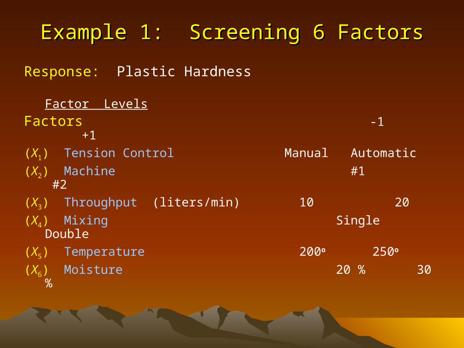
Example 1: Screening 6 FactorsExample 1: Screening 6 Factors

Response: Plastic Hardness Factor Levels

Factors -1 +1

(X1) Tension Control Manual Automatic

(X2) Machine #1 #2

(X3) Throughput (liters/min) 10 20

(X4) Mixing Single Double

(X5) Temperature 200o 250o

(X6) Moisture 20 % 30 %

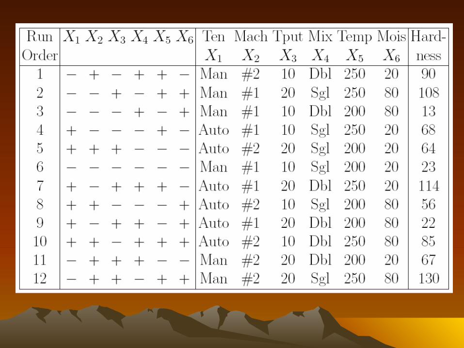
Randomly assign 6 columns to the 6 factors Randomly assign 6 columns to the 6 factors and then randomize the run orderand then randomize the run order

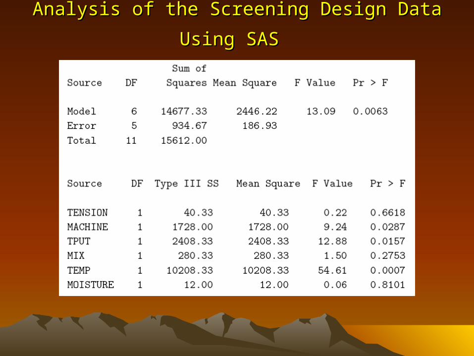
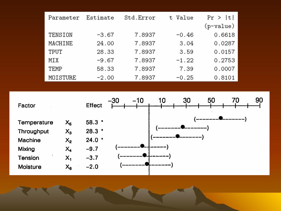
Analysis of the Screening Design Data Using SASAnalysis of the Screening Design Data Using SAS

3.3. 22kk Factorial ExperimentsFactorial Experiments

A 2k factorial design is a k-factor design such that The 2k experimental runs are the 2k

combinations of + and – factor levels Each factor has two levels coded + and -

The 2k experimental runs may also be replicated

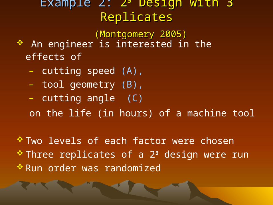
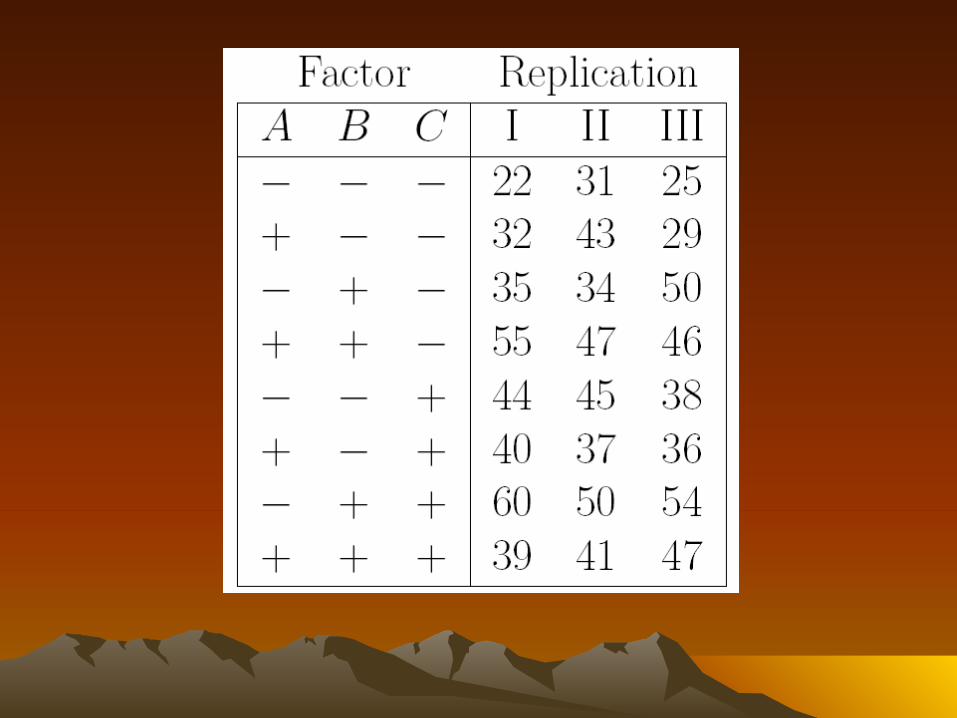
Example 2:Example 2: 2 233 Design with 3 Replicates Design with 3 Replicates (Montgomery 2005)(Montgomery 2005)

An engineer is interested in the effects of – cutting speed (A), – tool geometry (B), – cutting angle (C)

on the life (in hours) of a machine tool

Two levels of each factor were chosen Three replicates of a 23 design were run Run order was randomized

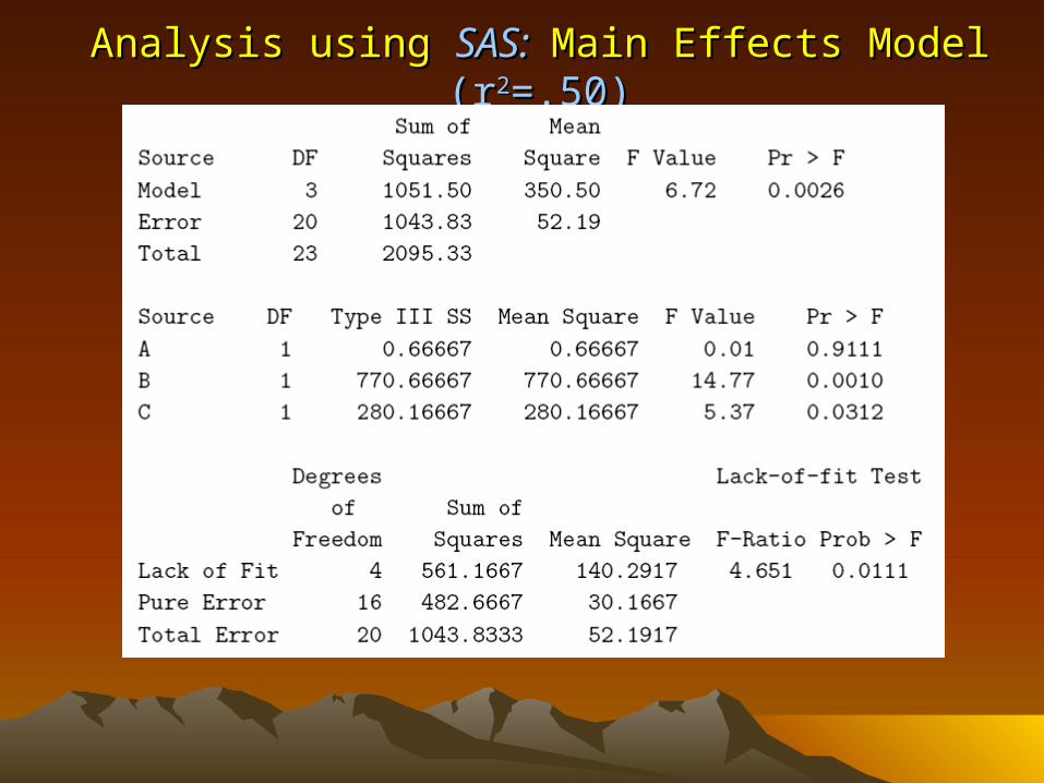
Analysis using Analysis using SAS: SAS: Main Effects Model Main Effects Model (r(r22=.50)=.50)

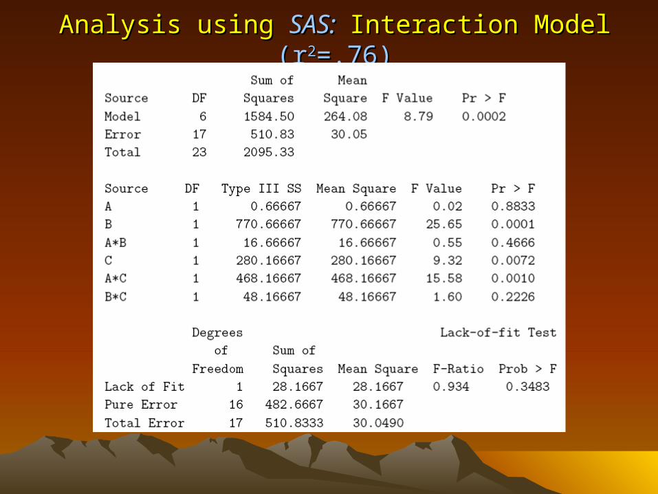
Analysis using Analysis using SAS: SAS: Interaction Model Interaction Model (r(r22=.76)=.76)

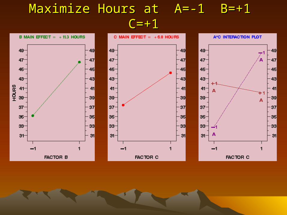
Maximize Hours at A=-1 B=+1 C=+1Maximize Hours at A=-1 B=+1 C=+1

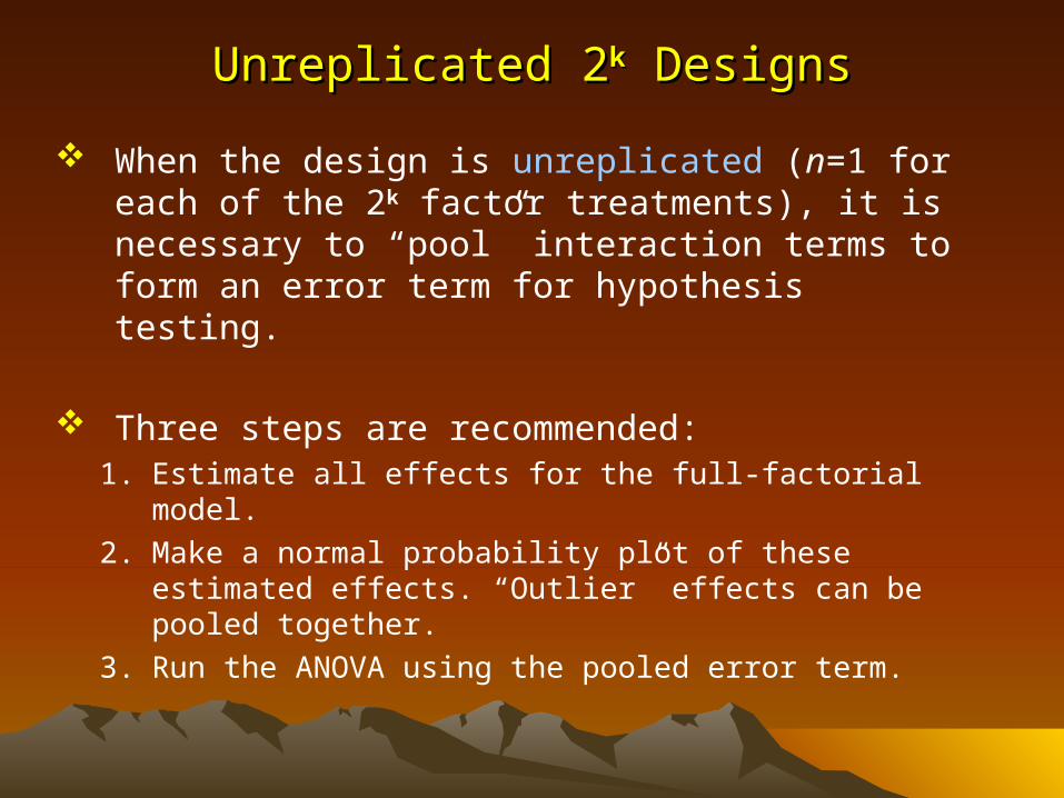
Unreplicated 2Unreplicated 2kk Designs Designs

When the design is unreplicated (n=1 for each of the 2k factor treatments), it is necessary to “pool” interaction terms to form an error term for hypothesis testing.

Three steps are recommended:1. Estimate all effects for the full-factorial model.

2. Make a normal probability plot of these estimated effects. “Outlier” effects can be pooled together.

3. Run the ANOVA using the pooled error term.

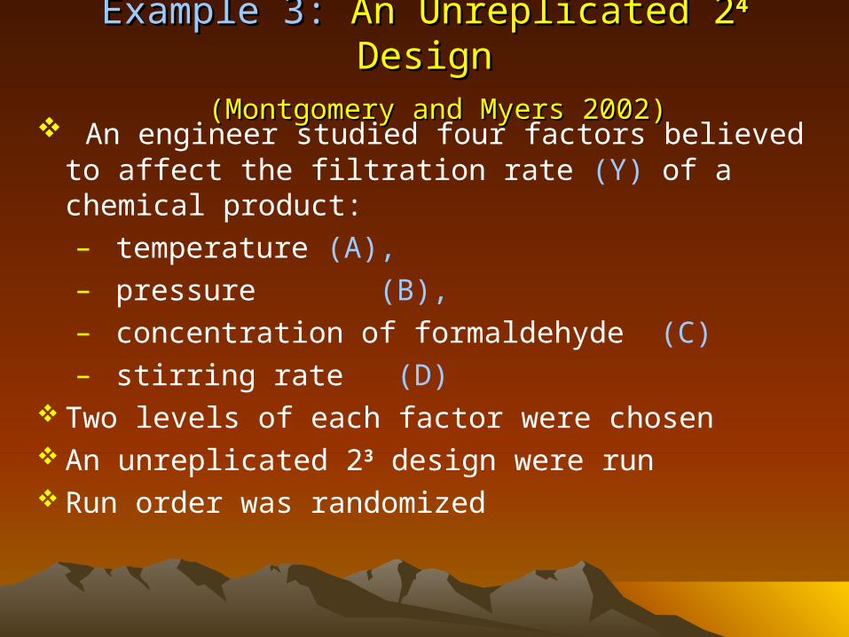
Example 3:Example 3: An Unreplicated 2 An Unreplicated 244 Design Design (Montgomery and Myers 2002)(Montgomery and Myers 2002)

An engineer studied four factors believed to affect the filtration rate (Y) of a chemical product:– temperature (A), – pressure (B), – concentration of formaldehyde (C) – stirring rate (D)

Two levels of each factor were chosen An unreplicated 23 design were run Run order was randomized

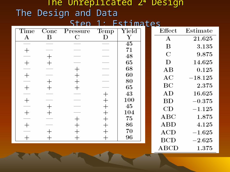
The Unreplicated 2The Unreplicated 244 Design DesignThe Design and Data Step 1: EstimatesThe Design and Data Step 1: Estimates

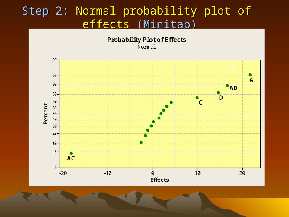
Step 2:Step 2: Normal probability plot of effects Normal probability plot of effects (Minitab)(Minitab)

Effects

Perc

ent

20100-10-20

99

95

90

80

70

605040

30

20

10

5

1

Probability Plot of EffectsNormal

AAD

DC

AC

A

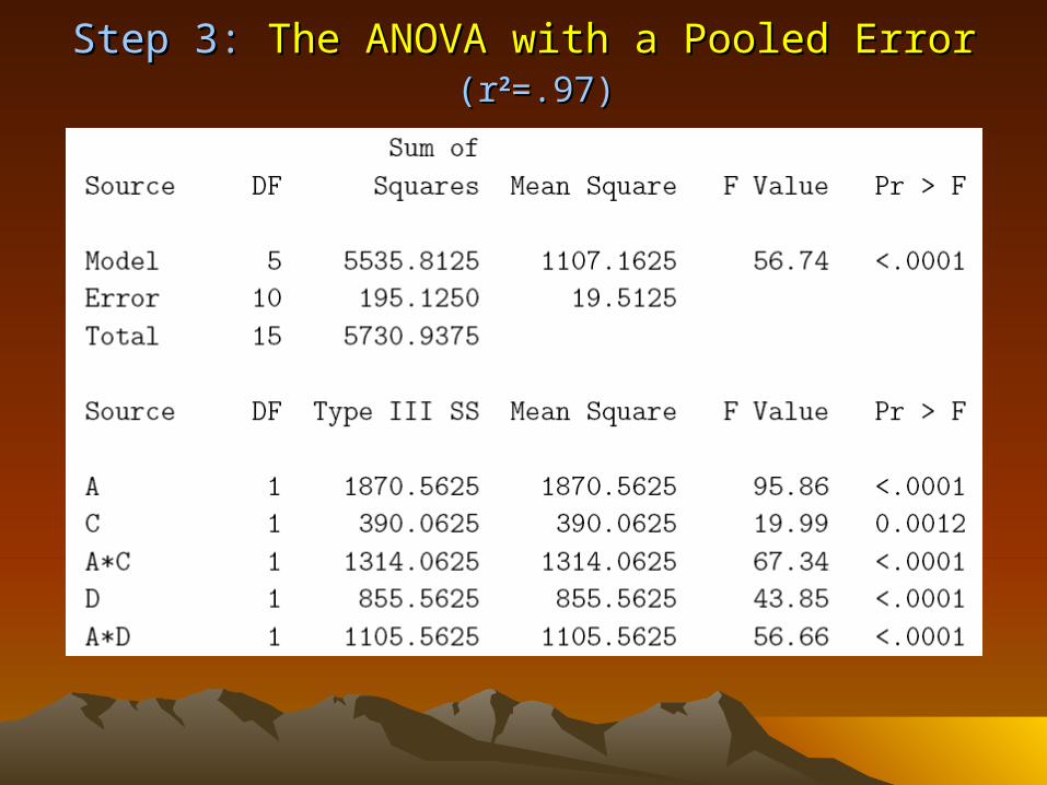
Step 3:Step 3: The ANOVA with a Pooled Error The ANOVA with a Pooled Error (r(r22=.97)=.97)

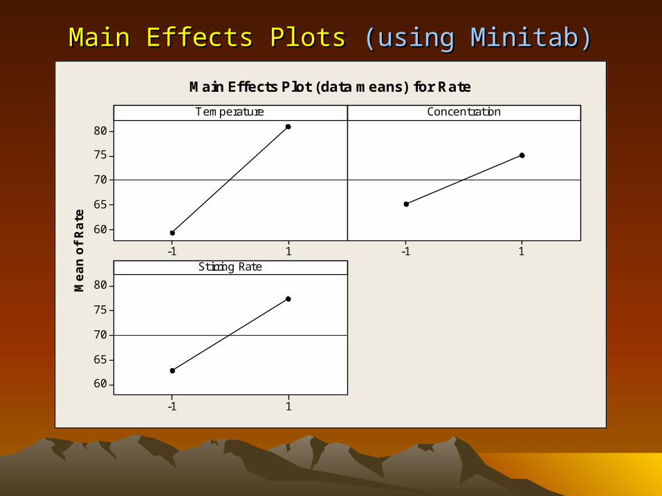
Main Effects Plots Main Effects Plots (using Minitab)(using Minitab)

Mean o

f Rate

1-1

80

75

70

65

60

1-1

1-1

80

75

70

65

60

Temperature Concentration

Stirring Rate

Main Effects Plot (data means) for Rate

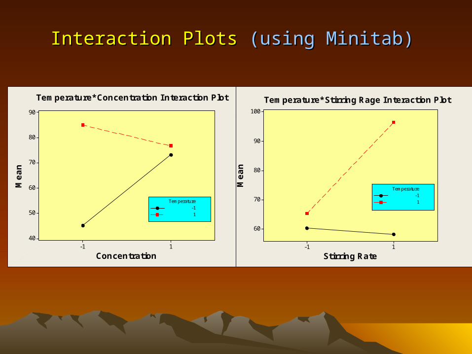
Interaction Plots Interaction Plots (using Minitab)(using Minitab)

Concentration

Mean

1-1

90

80

70

60

50

40

Temperature-11

Temperature*Concentration Interaction Plot

Stirring Rate

Mean

1-1

100

90

80

70

60

Temperature-11

Temperature*Stirring Rage Interaction Plot

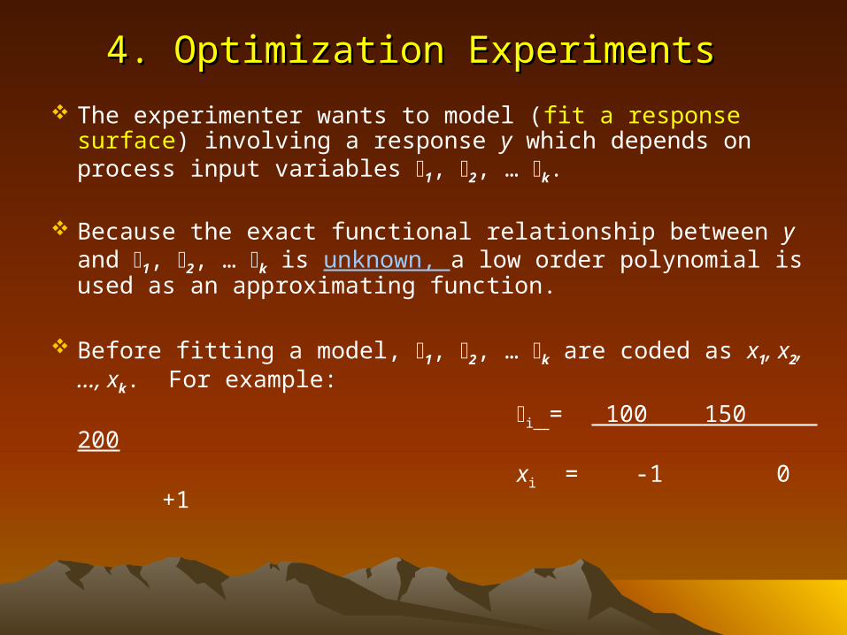
4. Optimization Experiments4. Optimization Experiments

The experimenter wants to model (fit a response surface) involving a response y which depends on process input variables 1, 2, … k.

Because the exact functional relationship between y and 1, 2, … k is unknown, a low order polynomial is used as an approximating function.

Before fitting a model, 1, 2, … k are coded as x1, x2, …, xk. For example:

i = 100 150 200

xi = -1 0 +1

4. Optimization Experiments4. Optimization Experiments

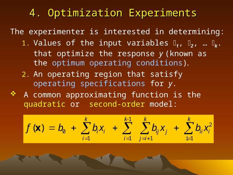
The experimenter is interested in determining:

1. Values of the input variables 1, 2, … k. that optimize the response y (known as the optimum operating conditions).

2. An operating region that satisfy operating specifications for y.

A common approximating function is the quadratic or second-order model:

2

1i1

1

110 )( i

k

iij

k

ijij

k-

ii

k

ii xbxbxbbf

x

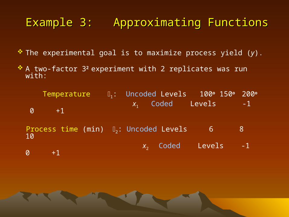
Example 3: Approximating FunctionsExample 3: Approximating Functions

The experimental goal is to maximize process yield (y).

A two-factor 32 experiment with 2 replicates was run with:

Temperature 1: Uncoded Levels 100o 150o 200o

x1 Coded Levels -1 0 +1

Process time (min) 2: Uncoded Levels 6 8 10 x2 Coded Levels -1 0 +1

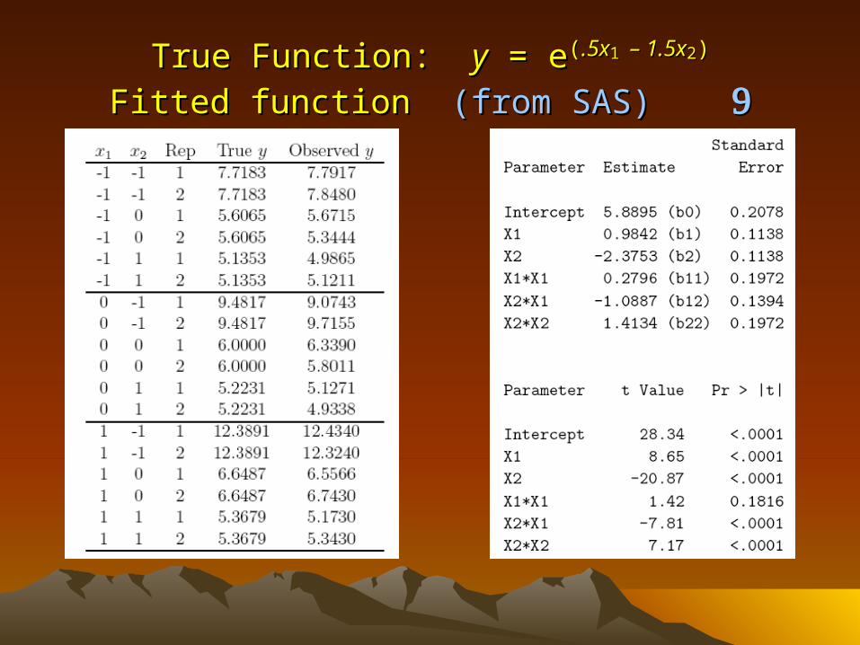
True Function: True Function: yy = e = e((.5x.5x11 – 1.5x– 1.5x22))

Fitted function Fitted function (from SAS) (from SAS)

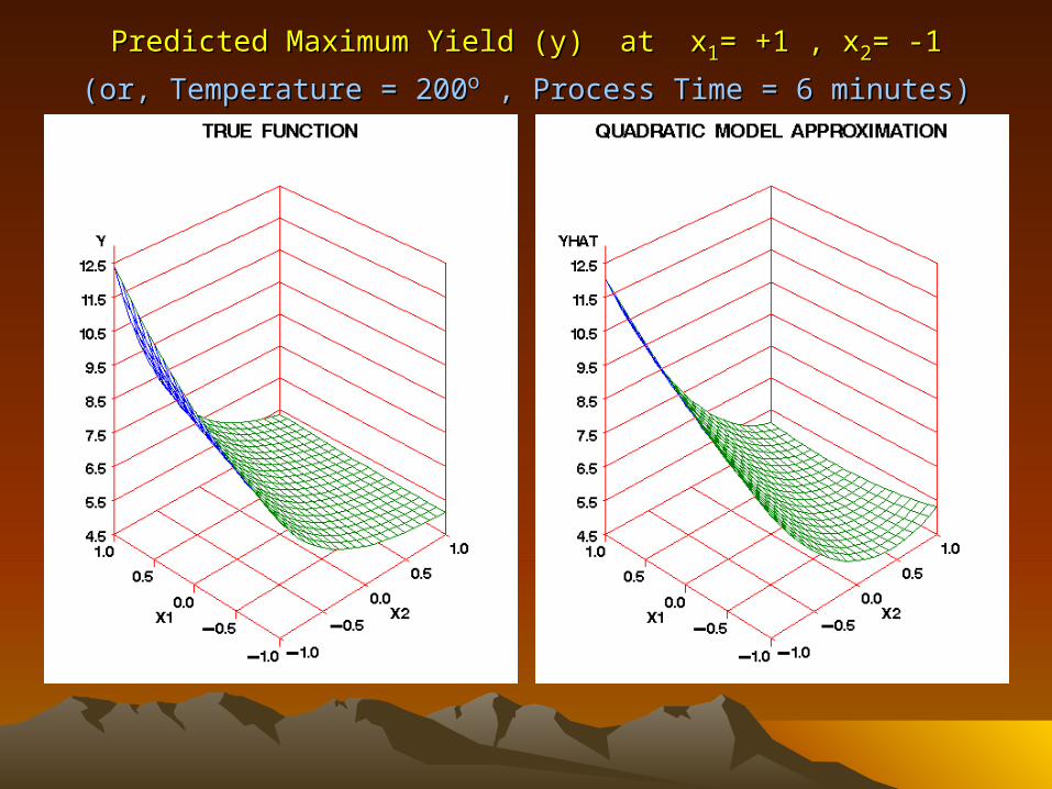
Predicted Maximum Yield (y) at xPredicted Maximum Yield (y) at x11= +1 , x= +1 , x22= -1= -1

(or, Temperature = 200(or, Temperature = 200oo , Process Time = 6 minutes) , Process Time = 6 minutes)

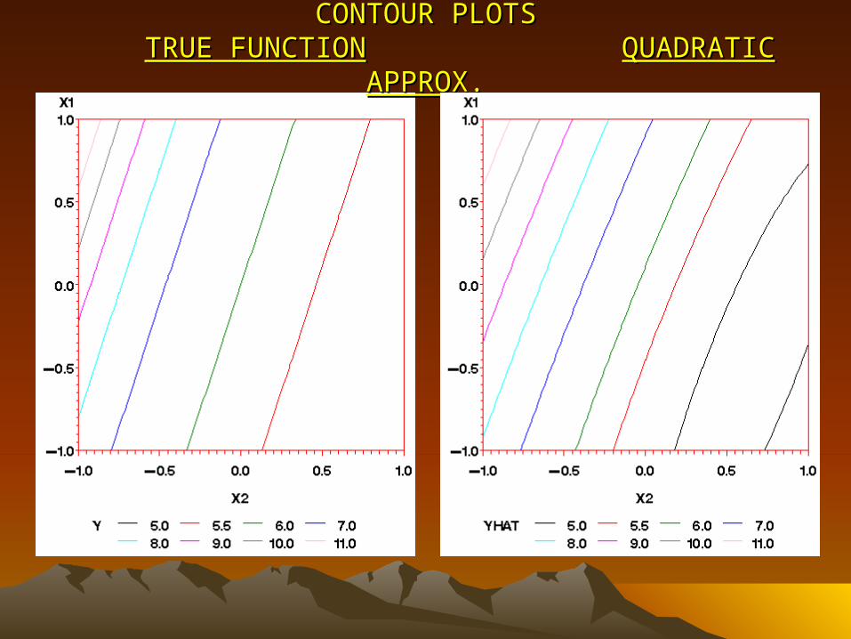
CONTOUR PLOTSCONTOUR PLOTS TRUE FUNCTIONTRUE FUNCTION QUADRATIC APPROX.QUADRATIC APPROX.

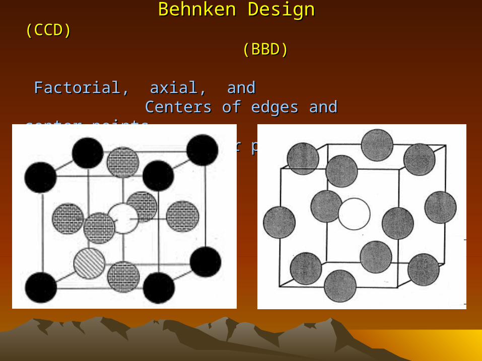
Central Composite Design Box-Behnken DesignCentral Composite Design Box-Behnken Design

(CCD) (BBD)(CCD) (BBD)

Factorial, axial, and Centers of edges andFactorial, axial, and Centers of edges andcenter points center pointscenter points center points

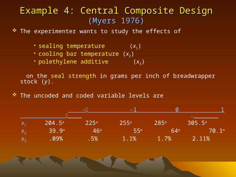
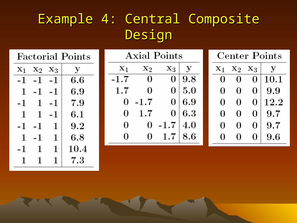
Example 4: Central Composite Design Example 4: Central Composite Design (Myers 1976)(Myers 1976)

The experimenter wants to study the effects of

• sealing temperature (x1) • cooling bar temperature (x2) • polethylene additive (x3)

on the seal strength in grams per inch of breadwrapper stock (y).

The uncoded and coded variable levels are

- -1 0 1 .

x1 204.5o 225o 255o 285o 305.5o

x2 39.9o 46o 55o 64o 70.1o

x3 .09% .5% 1.1% 1.7% 2.11%

Example 4: Central Composite DesignExample 4: Central Composite Design

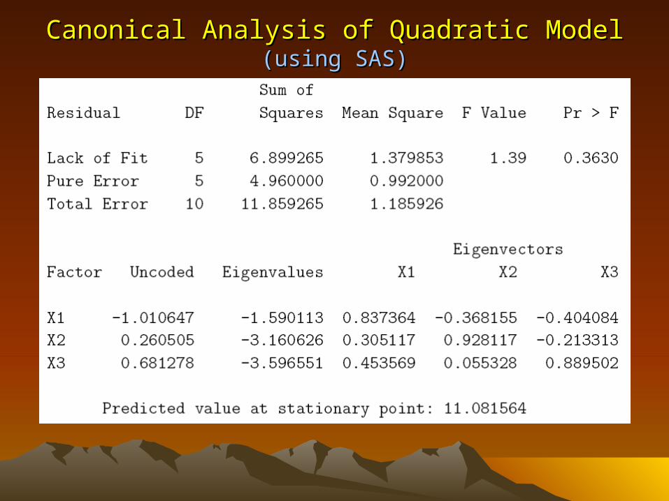
Canonical AnalysisCanonical Analysis of Quadratic Modelof Quadratic Model (using SAS)(using SAS)

Ridge AnalysisRidge Analysis of Quadratic Modelof Quadratic Model (using SAS)(using SAS)

Predicted Maximum atPredicted Maximum at x x11=-1.01 x=-1.01 x22=0.26 x=0.26 x33=0.68=0.68

5. Mixture Experiments5. Mixture Experiments

A mixture contains q components where xi is the proportion of the ith component (i=1,2,…, q)

Two constraints exist: 0 ≤ xi ≤ 1 and Σ xi = 1

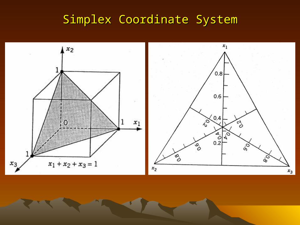
Simplex Coordinate SystemSimplex Coordinate System

Mixture Experiment ModelsMixture Experiment Models

Because the level of the final component can written as

xq = 1 – (x1 + x2 + + xq-1)

any response surface model used for independent factors can be reduced to a Scheffé model. Examples include:

Example of a 3-Component Mixture DesignExample of a 3-Component Mixture Design

Analysis of a 3-component Mixture ExperimentAnalysis of a 3-component Mixture Experiment

4-Component Mixture Experiment with Component Level 4-Component Mixture Experiment with Component Level Constraints Constraints (McLean & Anderson 1966)(McLean & Anderson 1966)

Response: Flare BrightnessResponse: Flare Brightness

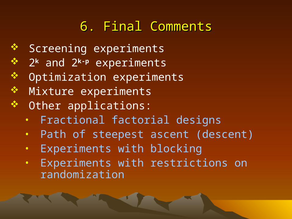
6. Final Comments6. Final Comments

Screening experiments 2k and 2k-p experiments Optimization experiments Mixture experiments Other applications:

• Fractional factorial designs• Path of steepest ascent (descent)• Experiments with blocking • Experiments with restrictions on randomization