Embed Size (px)
Citation preview
February 9th to June 19th, 2009National Institute of Informatics (Tokyo)
Inductive Logic Programming Applied to Systems Biology
Master Degree InternshipSynnaeve Gabriel
Advisors:Katsumi Inoue& Taisuke Sato
Contents
1 Introduction 3
2 Prerequisites and State of the Art 42.1 Molecular Biology: the Cell . . . . . . . . . . . . . . . . . . . . . . . . . . . . 4
2.1.1 Prokaryote and Eukaryote . . . . . . . . . . . . . . . . . . . . . . . . . 42.1.2 Energy . . . . . . . . . . . . . . . . . . . . . . . . . . . . . . . . . . . . 42.1.3 Material . . . . . . . . . . . . . . . . . . . . . . . . . . . . . . . . . . . 52.1.4 Metabolic Pathways . . . . . . . . . . . . . . . . . . . . . . . . . . . . . 5
2.2 Inductive Logic Programming . . . . . . . . . . . . . . . . . . . . . . . . . . . 72.2.1 Vocabulary, Notations & Definitions . . . . . . . . . . . . . . . . . . . 72.2.2 Overview . . . . . . . . . . . . . . . . . . . . . . . . . . . . . . . . . . . 72.2.3 Inverse Entailment for Abduction and Induction . . . . . . . . . . . . 82.2.4 CF-induction . . . . . . . . . . . . . . . . . . . . . . . . . . . . . . . . . 9
2.3 Previous and Related Works . . . . . . . . . . . . . . . . . . . . . . . . . . . . 102.3.1 Analytical Models and Quantitative Analysis . . . . . . . . . . . . . . 102.3.2 Logic Based Approaches . . . . . . . . . . . . . . . . . . . . . . . . . . 112.3.3 Japanese-French Symposium on Systems Biology . . . . . . . . . . . 12
3 Discrete Levels and Kinetic Modeling of Reactions 143.1 Precision – Generality trade-off . . . . . . . . . . . . . . . . . . . . . . . . . . 143.2 Introducing Discrete Levels (in the Symbolic Modeling) . . . . . . . . . . . . 16
3.2.1 Time Series Discretization . . . . . . . . . . . . . . . . . . . . . . . . . 163.2.2 Our approach . . . . . . . . . . . . . . . . . . . . . . . . . . . . . . . . 17
3.3 Michaelis-Menten Kinetics . . . . . . . . . . . . . . . . . . . . . . . . . . . . 183.3.1 Establishing Michaelis-Menten Equation . . . . . . . . . . . . . . . . 183.3.2 Simplification . . . . . . . . . . . . . . . . . . . . . . . . . . . . . . . . 19
4 Implementations and Results 214.1 kegg2symb: Automatic Conversion of Pathways . . . . . . . . . . . . . . . . 214.2 Discrete Levels . . . . . . . . . . . . . . . . . . . . . . . . . . . . . . . . . . . 21
4.2.1 Hidden Markov Models . . . . . . . . . . . . . . . . . . . . . . . . . . . 214.2.2 Parameter Tying . . . . . . . . . . . . . . . . . . . . . . . . . . . . . . 224.2.3 Expectation-Maximization and Variational Bayes EM . . . . . . . . . 234.2.4 Discretization Process . . . . . . . . . . . . . . . . . . . . . . . . . . . 25
4.3 Logic Model . . . . . . . . . . . . . . . . . . . . . . . . . . . . . . . . . . . . . 264.3.1 Modeling of the Pathway . . . . . . . . . . . . . . . . . . . . . . . . . . 264.3.2 Abducing hypotheses with SOLAR . . . . . . . . . . . . . . . . . . . . 274.3.3 Kinetic Modeling . . . . . . . . . . . . . . . . . . . . . . . . . . . . . . 29
4.4 Results . . . . . . . . . . . . . . . . . . . . . . . . . . . . . . . . . . . . . . . . 304.4.1 Ranking the Hypotheses with BDD-EM . . . . . . . . . . . . . . . . . 304.4.2 Choosing the Hypotheses . . . . . . . . . . . . . . . . . . . . . . . . . 314.4.3 Interpretation . . . . . . . . . . . . . . . . . . . . . . . . . . . . . . . . 32
5 Possible Extensions of this Work 345.1 Kinetic Modeling . . . . . . . . . . . . . . . . . . . . . . . . . . . . . . . . . . 345.2 Building other Models . . . . . . . . . . . . . . . . . . . . . . . . . . . . . . . 355.3 Hypothesis Finding . . . . . . . . . . . . . . . . . . . . . . . . . . . . . . . . . 36
0.0 ILP Applied to Systems Biology Gabriel Synnaeve
6 Conclusion 37
Acknowledgements 38
References 39
Glossary 42
Appendix 436.1 (Short) Example of the discretization of a time series . . . . . . . . . . . . . 446.2 Glycolysis & Pentose Phosphate Pathway for E.Coli . . . . . . . . . . . . . . 446.3 ILP 2009 Poster . . . . . . . . . . . . . . . . . . . . . . . . . . . . . . . . . . . 486.4 Discovery Science 2009 submission . . . . . . . . . . . . . . . . . . . . . . . . 48
sssssKeywords:
inductive logic programming, molecular biology, systems biology, abduction, hypothesisfinding, Michaelis-Menten kinetics, cell, bioengineering, inverse entailment, consequencefinding, hidden Markov models, expectation-maximization algorithm, variational Bayes,binary decision diagrams, knowledge discovery process ...
Foreword:
This internship report is intended to an university jury but, more than that, the authorconsidered to make it useful in another way: he would be very pleased if it could helpsomeone (anybody) new in the research domain of “hypothesis finding for systems biologythrough logic-based methods”. The content is intended to fullfill the absolutely basic re-quirements for entering the related research topics as well as giving the central referencesand showing the thought process that lead to such a conclusion.
2
1.0 ILP Applied to Systems Biology Gabriel Synnaeve
1 Introduction
This internship is being done at the National Institute of Informatics (NII, Tokyo) underthe supervising of Katsumi Inoue (NII) and Taisuke Sato (Tokyo Institute of Technology).The corresponding French advisor is Pierre Bessiere (CNRS, Grenoble). The subject ofthe internship deals with the hypothesis finding (knowledge discovery) process for sys-tems biology through inductive logic programming. The goal is to enhance the modelingof metabolic pathways of cells in order to obtain good predictive in silico models that willtake all the mutual interactions of metabolites into account. The interest is to give abetter understanding of the physiological state of the cell by improving the interpretationof the interactions between metabolic and signaling networks. The application fieldsrange from biochemical engineering of proteins to the comprehension of cell aging (can-cers) and drugs side effects prediction.
Systems biology is the discipline that studies biology at the molecular level by con-sidering the cell as a complex system constituted of internal chemical interactions. Thebehavior of such a biological system is predicted from the point of view of a complex sys-tem involving time and non-linearity. The size and the non-linearity of the models of thecell’s metabolisms forces us to predict some parameters that can’t be measured. Someparameters can be measured in vitro but not in vivo and their values vary a lot because ofall the external interaction of in vivo experiences. Numerical data is obtained at differentlevels: macroscopic, microscopic and molecular, and from different experiences. This leadsus to set a threshold level between precision and generality by applying discretization.
Inductive logic programming is a machine learning technique that we use on ex-perimental (sometimes incomplete) data for hypothesis finding. It allows us to computeeither missing values (facts) or more general rules that explain some observations givena background knowledge. Finding missing facts is called abduction, and building rules(through generalization of clauses) is called induction. This techniques are very powerfulto deal with the amount of experimental data and the increase of background knowledgein systems biology every year. Indeed, today’s advances in data acquisition and handlingtechnologies provides a wealth of new data that should lead to more predictive and com-prehensive models. Besides, one can easily increment the background knowledge of agiven model by adding computed rules or abducibles to it.
Logical kinetic models of the glycolysis and pentose phosphate pathways of Es-cherichia Coli and Saccharomyces Cerevisiae have been developped in order to study themetabolic response of a biological system after the injection of a pulse of glucose. Thedescription of the internship’s work follows this pattern: we will first explain the basicbiological knowledge required to deal with metabolic pathways and explain the inductivelogic programming framework. Then, we will draw a state of the art showing the cur-rent problems that scientists encounter. We will then explain our kinetic based approachand justify its use and the need for discrete levels. We finish by discussing the imple-mentation and the results of logical abduction of the concentrations of metabolites beforethe dynamic transition. Before concluding, we will open on future works that are nowpossible.
3
2.1 ILP Applied to Systems Biology Gabriel Synnaeve
2 Prerequisites and State of the Art
What makes the wealth and the complexity of a cell is on the one hand its numerousgenes, and on the other hand the degree of interactions between its different chemicalcompounds (protein-protein, protein-ADN, protein-metabolite). It is therefore necessaryto make an analysis taking into account the totality of interactions. For instance, if thedatabases concerning the Escherichia Coli increase each year with new results about thediscovery of new proteins and new behavior due to some expressed genes, the mathemati-cal modeling of the prokaryote cells is always an open question which excite the scientificcommunity. Nowadays, bioinformatics represents the key field to explain the functionalityof lifescience. To analyze a biological system it is necessary to find out new mathematicalmodels allowing to explain the evolution of the system in a dynamic context [Kitano 02].Many physical and biological phenomena may be represented on an analytical form usinga dynamical system. The majority of kinetic models in biology are described by coupleddifferential equations and simulators are implemented with the appropriate methods tosolve these systems. However, for most nonlinear dynamical systems it is difficult to findan analytical solution. The understanding of the phenomenon described by a complexsystem is carried out by a qualitative study of its behaviour such as stability or forking.The qualitative analysis based on perturbation method is a difficult task and is oftenperformed by decomposition in subsystems which are simulated numerically.
2.1 Molecular Biology: the Cell
Basically, there are two types of cells but both have to provide functions and to reproduce.Both require a lot of intermediate steps that make use of energy and material.
2.1.1 Prokaryote and Eukaryote
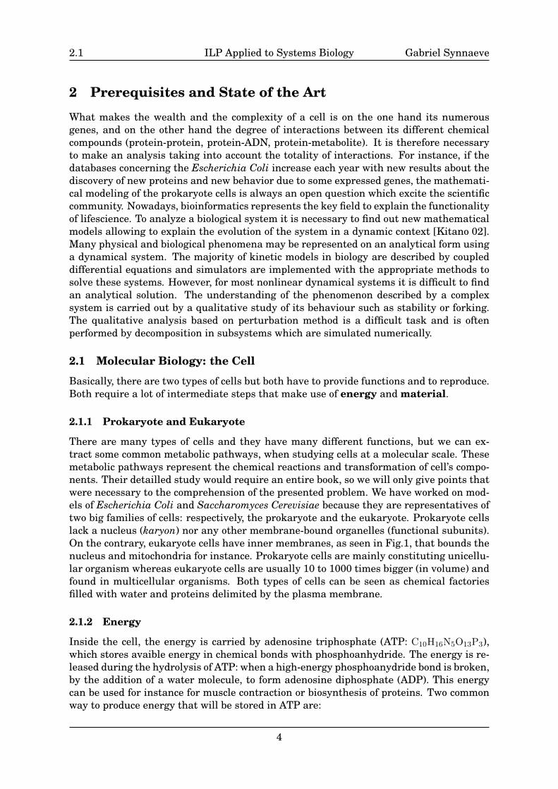
There are many types of cells and they have many different functions, but we can ex-tract some common metabolic pathways, when studying cells at a molecular scale. Thesemetabolic pathways represent the chemical reactions and transformation of cell’s compo-nents. Their detailled study would require an entire book, so we will only give points thatwere necessary to the comprehension of the presented problem. We have worked on mod-els of Escherichia Coli and Saccharomyces Cerevisiae because they are representatives oftwo big families of cells: respectively, the prokaryote and the eukaryote. Prokaryote cellslack a nucleus (karyon) nor any other membrane-bound organelles (functional subunits).On the contrary, eukaryote cells have inner membranes, as seen in Fig.1, that bounds thenucleus and mitochondria for instance. Prokaryote cells are mainly constituting unicellu-lar organism whereas eukaryote cells are usually 10 to 1000 times bigger (in volume) andfound in multicellular organisms. Both types of cells can be seen as chemical factoriesfilled with water and proteins delimited by the plasma membrane.
2.1.2 Energy
Inside the cell, the energy is carried by adenosine triphosphate (ATP: C10H16N5O13P3),which stores avaible energy in chemical bonds with phosphoanhydride. The energy is re-leased during the hydrolysis of ATP: when a high-energy phosphoanydride bond is broken,by the addition of a water molecule, to form adenosine diphosphate (ADP). This energycan be used for instance for muscle contraction or biosynthesis of proteins. Two commonway to produce energy that will be stored in ATP are:
4
2.1 ILP Applied to Systems Biology Gabriel Synnaeve
Eukaryote Prokaryote
Nucleus
Nucleolis MitochondriaNucleoid
Capsule
FlagellumCell Wall
Cell MembraneRibosomes
Figure 1: Cell types: left: eukaryote, right: prokaryote
• glycolysis: the degradation of glucose (C6H12O6 for instance) in carbon dioxide (CO2)and water (H2O). The energy emitted by cutting chemical bonds is stored into ATPand reduced nicotinamide adenine dinucleotide (NADH).
• photosynthesis: the conversion of carbon dioxide and water into organic compounds(especially sugars) and oxygen (waste product) using solar energy. A part of the lightenergy absorbed by chlorophylls is stored in ATP.
2.1.3 Material
The universal material of the cell are proteins, which are complex molecules made from20 basic amino-acids, 8 of them cannot be synthetised by human cells. Proteins form theinternal skeleton and membrane of the cell. Other proteins can be (non-exhaustive list)sensors, intracellular messages, extracellular signals, enzymes (catalysing chemical re-actions), motors, control gene activity (transcription factors) and carry substances acrossthe plasma membrane. In a liver cell, protein accounts for approximately 20% of theweight with an approximative 7.0 × 10⁹ total number of protein molecules per liver cell.The mean protein is 400 amino-acids long.
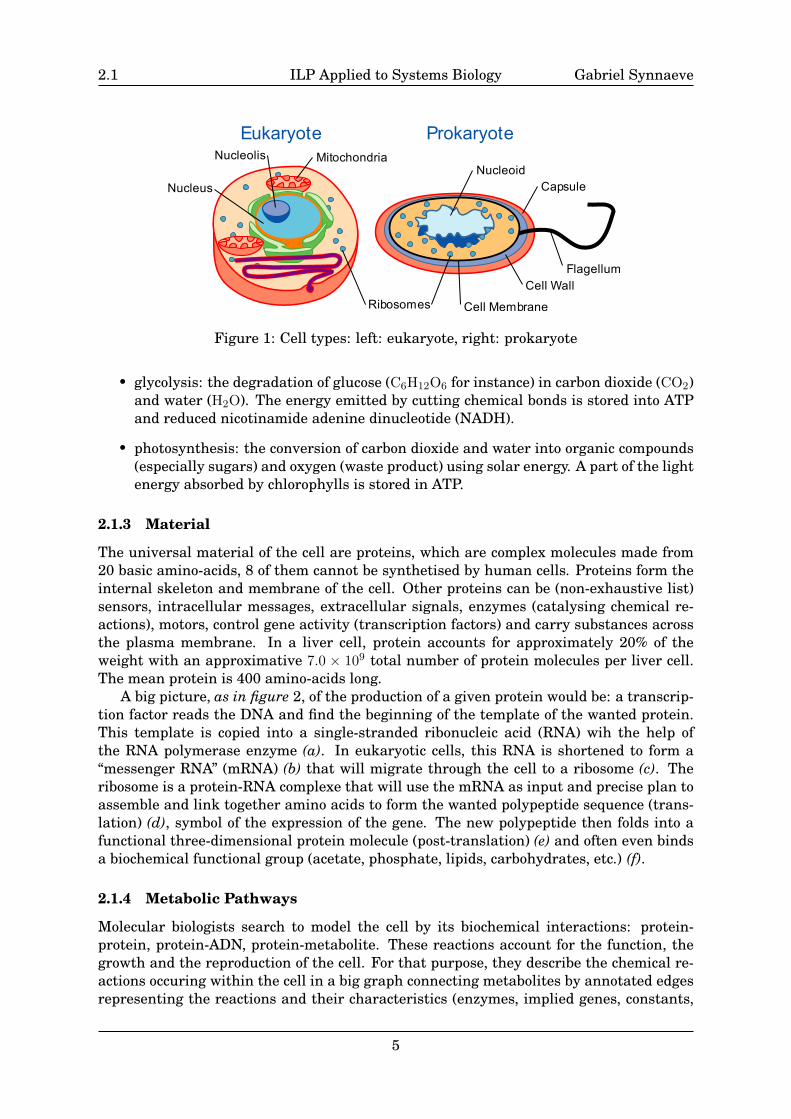
A big picture, as in figure 2, of the production of a given protein would be: a transcrip-tion factor reads the DNA and find the beginning of the template of the wanted protein.This template is copied into a single-stranded ribonucleic acid (RNA) wih the help ofthe RNA polymerase enzyme (a). In eukaryotic cells, this RNA is shortened to form a“messenger RNA” (mRNA) (b) that will migrate through the cell to a ribosome (c). Theribosome is a protein-RNA complexe that will use the mRNA as input and precise plan toassemble and link together amino acids to form the wanted polypeptide sequence (trans-lation) (d), symbol of the expression of the gene. The new polypeptide then folds into afunctional three-dimensional protein molecule (post-translation) (e) and often even bindsa biochemical functional group (acetate, phosphate, lipids, carbohydrates, etc.) (f).
2.1.4 Metabolic Pathways
Molecular biologists search to model the cell by its biochemical interactions: protein-protein, protein-ADN, protein-metabolite. These reactions account for the function, thegrowth and the reproduction of the cell. For that purpose, they describe the chemical re-actions occuring within the cell in a big graph connecting metabolites by annotated edgesrepresenting the reactions and their characteristics (enzymes, implied genes, constants,
5
2.2 ILP Applied to Systems Biology Gabriel Synnaeve
a b
RNA
mRNA
DNA
c
d
e
f
effector molecule
ribosome polypeptidesequence
protein
Figure 2: Protein synthesis originates in the nucleus (blue) and finish in the cytoplasm(beige). a: transcription ; b: post-transcription ; c: migration of the mRNA into thecytoplasm ; d: translation ; e: post-translation / folding ; f: binding of an effector
etc.): these interconnected reactions are forming a metabolic pathway. The substrates(reactants) of one reaction are the products of the previous one. All reactions are chemi-cally reversible, but the thermodynamical conditions in the cell often favorise one direc-tion. There are two types of metabolic pathways: catabolic ones, that break down inputmolecules to store energy, and anabolic ones, that construct big molecules from smallerunits.
You can see an example of a metabolic pathway in appendix: Fig.24 from the KyotoEncyclopedia of Genes and Genomes (KEGG) [Kanehisa & Goto 00, Kanehisa et al. 08].This is the glycolysis pathway: glucose (C6H12O6) enters the cell and is phosphorylatedby ATP to glucose 6-phosphate (G6P) in order not to be able to leave the cell. The “goal”of the pathway is then to produce pyruvate (C3H4O−3 ) from this G6P and store the energyreleased when cutting bounds into ATP and NADH. This pathway can run in reverse toproduce G6P for storage: in this case, it is called glucogenesis. Metabolic pathways areoften regulated by inhibitions of some of the enzymes or by internal cycles (as the Krebscycle, that is denoted as citrate cycle in Fig.24). Such metabolic pathways are specialisedfor each cell with some specific reactions and different protein syntheses.
Metabolic engineering tries to produce metabolites such as amino acids, vitamins, or-ganic acids, etc. from biochemical synthesis. It is crucial to understand (to be able to con-trol) the flux distribution, regulation phenomena and control properties of the interestingmetabolism [Doncescu et al. 07]. As intracellular fluxes cannot be measured, they arecomputed by solving a set of linear equations consisting of the mass balances equationsof the intracellular metabolites. S[m metabolites × n reactions] being the stoichiometricmatrix of the metabolic network, v = (v1, v2, . . . , vn) the unknown fluxes of the n reactions,C = (C1, C2, . . . , Cm) the concentration of the m metabolites and r the accumulation rateof metabolites, we have:
S.v =dC
dt= r (2.1)
In metabolic engineering, the system is considered to be able to reach steady states: whenthe input flux is equal to the ouput one, so when r = 0. It is then possible to computev. Therefore, determining the structure of a metabolic network and its steady states isthe first step towards the biosynthesis of molecules of interest and it is needed to build akinetic model for in silico analysis of the metabolism.
6
2.2 ILP Applied to Systems Biology Gabriel Synnaeve
2.2 Inductive Logic Programming
This (sub)section is mainly based on the Machine Learning 2004 paper from KatsumiInoue: Induction as Consequence Finding [Inoue 04]. This is only boiled down to the es-sentials to have an overview of how are constructed the hypotheses in the following parts.
2.2.1 Vocabulary, Notations & Definitions
A clause is a disjunction of literals: C = {A1, . . . , Am,¬B1, . . . ,¬Bn}, with atomic Ai, Bi,can also be noted C = {B1 ∧ · · · ∧ Bn ⊃ A1 ∨ · · · ∨ Am}. The empty clause is noted �. Apositive (negative) clause is a clause whose disjuncts are all positive (negative) litterals. Anegative clause can also be named an integrity constraint. A Horn clause is a definite (onlyone positive litteral) or negative clause. Ex: C ′ = {¬B1, . . . ,¬Bn, A} = {B1∧ · · ·∧Bn ⇒ A}is Horn (otherwise, it’s non-Horn). A unit clause is a clause of length 1, only 1 litteral. Aconjunctive normal form (CNF) is a conjunction of clauses, and a disjunctive normal form(DNF) is a disjunction of conjunctions of literals. A clausal theory Σ is a finite set (CNF)of clauses. If a clausal theory contains only Horn clauses, it is a Horn program, otherwise,the clausal theory is said to be full (with non-Horn clauses). A clause C subsumes a clauseD if and only if (iff) there is a substitution θ such that Cθ ⊆ D. C is then told to be moregeneral than D. C properly subsumes D iff C subsumes D but D does not subsume C.µΣ denotes the set of clauses in a clausal theory Σ that are not properly subsumed byany other clause in Σ (µ stands for “minimal subsumption”). For a clausal theory Σ, aconsequence of Σ is a clause entailed by Σ. The set of all consequences of Σ is noted Th(Σ).Completeness refers to the ability to prove any formula that is true. Consistency refersto the impossibility to prove both P and ¬P at the same time. A production field is a pair[L, Cond], where L is a set of literals closed under instanciation, and Cond is a conditionto be satisfied. For instance P = [p( , , )+, length ≤ 1 and term depth ≤ 1] could be usedto set the abductive bias by asking for the hypotheses to follow that form, where p( , , )+
is the set of all positive literal whose predicate symbol is p and takes 3 arguments, andsatisfy this conditions. A production field P is stable if, for any two clauses C and D suchthat C ⊆ D, D ∈ P only if C ∈ P.
2.2.2 Overview
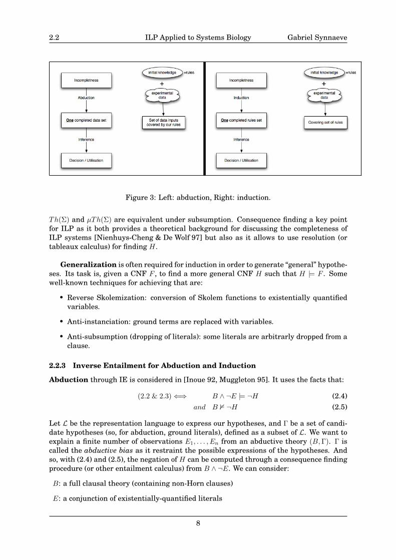
Both induction and abduction are part of the inductive logic programming (ILP) frame-work [Mooney 97]. Their goals (see Fig.3) are to seek hypotheses that (2.2) account forgiven observations or examples while (2.3) staying consistent with the background. Givena background theory B and positive examples E (both are clausal theories), the task ofinduction and abduction is to find an hypothesis H such that:
B ∧H |= E (2.2)and B ∧H 2 ⊥ (2.3)
Abduction infers direct causes of observations, like missing facts (that hasn’t been ob-served), that are often called explanations. Induction focuses more on finding gen-eral hypotheses that cover as many positive examples as possible (and as less nega-tive ones as possible). Their relation and interactions are studied more in depth in[Flach & Kakas 00].
The resolution is complete for consequence finding [Lee 67] and even C |= D can be re-placed by C ⊆ D (subsumes). With Σ |=resolution Th(Σ)⇒ Σ ⊆ Th(Σ), Σ |= µΣ and µΣ ⊆ Σ:
7
2.2 ILP Applied to Systems Biology Gabriel Synnaeve
Figure 3: Left: abduction, Right: induction.
Th(Σ) and µTh(Σ) are equivalent under subsumption. Consequence finding a key pointfor ILP as it both provides a theoretical background for discussing the completeness ofILP systems [Nienhuys-Cheng & De Wolf 97] but also as it allows to use resolution (ortableaux calculus) for finding H.
Generalization is often required for induction in order to generate “general” hypothe-ses. Its task is, given a CNF F , to find a more general CNF H such that H |= F . Somewell-known techniques for achieving that are:
• Reverse Skolemization: conversion of Skolem functions to existentially quantifiedvariables.
• Anti-instanciation: ground terms are replaced with variables.
• Anti-subsumption (dropping of literals): some literals are arbitrarly dropped from aclause.
2.2.3 Inverse Entailment for Abduction and Induction
Abduction through IE is considered in [Inoue 92, Muggleton 95]. It uses the facts that:
(2.2 & 2.3)⇐⇒ B ∧ ¬E |= ¬H (2.4)and B 2 ¬H (2.5)
Let L be the representation language to express our hypotheses, and Γ be a set of candi-date hypotheses (so, for abduction, ground literals), defined as a subset of L. We want toexplain a finite number of observations E1, . . . , En from an abductive theory (B,Γ). Γ iscalled the abductive bias as it restraint the possible expressions of the hypotheses. Andso, with (2.4) and (2.5), the negation of H can be computed through a consequence findingprocedure (or other entailment calculus) from B ∧ ¬E. We can consider:
B: a full clausal theory (containing non-Horn clauses)
E: a conjunction of existentially-quantified literals
8
2.2 ILP Applied to Systems Biology Gabriel Synnaeve
H: a conjunction of literals (within the abductive bias)
With respect to this, the IE calculus is sound and complete for computing abductive ex-planations.
IE for induction was first considered in [Muggleton 95] with the Progol system. Theprinciple that it introduced for induction as IE is to work with a “bridge” formula U suchthat
B ∧ ¬E |= U, U |= ¬H (2.6)
IE for induction as in [Muggleton 95] uses the bottom clause (conjunction of all unitclauses entailed by B ∧ ¬E) as “bridge” formula:
⊥(B,E) = {¬L|L is a literal and B ∧ ¬E |= L} (2.7)
and a hypothesis H is constructed by generalizing a sub-clause of ⊥(B,E):
H |= ⊥(B,E) (2.8)
The negation of H can be computed through a consequence finding procedure. We canconsider:
B: a Horn program
E: a Horn clause
H: a Horn clause
With respect to this, the IE calculus is sound (correct) but incomplete [Yamamoto 97] forcomputing inductive hypotheses.
2.2.4 CF-induction
By extending the notion of consequence finding, [Inoue 92] defined characteristic clausesto represent “interesting” clauses for a given problem. For a clausal theory Σ, the set oflogical consequence of Σ belonging to the production field P is denoted as ThP(Σ). Thecharacteristic clauses of Σ with respect to P are defined as:
Carc(Σ,P) = µThP)(Σ) (2.9)
Which leads to Carc(Σ,P) = {�} ⇔ Σ is unsatisfiable and P is stable. For instance, whenΣ = (¬p ∨ q) ∧ p:
Carc(Σ,LΣ) = p ∧ q
There are several procedures to compute characteristic clauses (through the elegantNewCarc:new characteristic clauses expansion) that can be found in [Inoue 92] and [Inoue 04].
CF-induction (as induction in the large) is interested in the formulas derived fromB ∧ ¬E that are not derived from B alone. Instead of ⊥(B,E), it considers some clausaltheory CC(B,E) as a “bridge” formula. (2.4) and (2.5) can then be rewritten as:
B ∧ ¬E |= CC(B,E) (2.10)CC(B,E) |= ¬H (⇐⇒ H |= ¬CC(B,E)) (2.11)
9
2.3 ILP Applied to Systems Biology Gabriel Synnaeve
CC(B,E) is obtained by consequence finding from the characteristic clauses of B ∧ ¬Ebecause (by definition of Carc) any other consequence of B ∧ ¬E belonging to P can beobtained by constructing a clause that is subsumed by a characteristic clause. Hence, wehave:
Carc(B ∧ ¬E,P) |= CC(B,E) (2.12)
with P giving an inductive bias. In (2.11), we have ¬CC(B,E) as DNF, it should beconverted into the CNF formula F which H entails:
F ≡ ¬CC(B,E) (2.13)H |= F (2.14)
Finishing the process of CF-induction from (2.13) is only to generalize (see page 8) theclausal theory F to H such that B ∧ H is consistent and H is Skolem free (withoutSkolem terms, i.e. without constants that could be replaced by existentially quantifiedvariables).
CF-induction can be tracted to a consequence finding procedure and consider the mostgeneral class:
B: a full clausal theory
E: a full clausal theory
H: a full clausal theory
The IE calculus is sound (correct) and complete for computing inductive hypotheses.
2.3 Previous and Related Works
“To understand biology at the system level, we must examine the structureand dynamics of cellular and organismal function, rather than thecharacteristics of isolated parts of a cell or organism.” [Kitano 02]
2.3.1 Analytical Models and Quantitative Analysis
There are analytical models of cells’ metabolisms, which are organised as complex net-works of interconnected reactions, where the global behavior is the result of individualproperties of enzymes, stoichiometry, metabolites, reactions constants. The approachesare based on mass-balance and/or kinetic methods which also account for dynamic behav-ior. The choice of Michaelis-Menten formalism has often been made as a representationof a non-linear allosteric regulation system.
Dynamic models are often based on integral and (ordinary) differential equations(ODEs). In [Waser et al. 83], the authors study the kinetics of the phosphofructokinasereaction (part of the glycolysis pathway) through the use of ODE. They used mainly Hill’skinetics for the regulation of the enzymatic activity. A work that is closer to what wehave done can be found in [Franco & Canela 84], where the authors simulate the purinemetabolism by ODEs (one equation per reaction-enzyme couple) using the Michaelis con-stant of each enzyme. The results that we have for the experiment of a pulse of glu-cose on Saccharomyces Cerevisiae are based on an simulator from Andrei Doncescuusing integral / differential equations. This is a work based on experimental data and
10
2.3 ILP Applied to Systems Biology Gabriel Synnaeve
[Mauch et al. 00] where the authors describe the experiments, assumptions and modelingin details. Not every quantitative analysis is done through ODE. For instance, the pa-per [Hofestadt & Thelen 98] presents a quantitative simulation of biochemical networkswhile using Petrinets.
In [Reder 88], the author has emphasized on the structural characterization and prop-erties of the metabolic network as opposed to the reaction kinetics. This is not directlyrelated to the current work, but this is an interesting approach of a very related problem.More generally, the analytical models are designed to have a very precise modeling of thecell (or part of it) but lack a global approach that would allow to find “general” formulasthat rule this complex system. Also, it is not always possible to measure the evolutionof concentration of metabolites in vivo, but parameters of ODEs (or other quantitative)models are sometimes approximated by in vitro measurements. This can be a source oferror as they can differ a lot from in vivo numbers. This is why logic based approaches(and mixed ones) exist: it should be better at handling general cases and structural drivenrules.
2.3.2 Logic Based Approaches
In [Tamaddoni-Nezhad et al. 06], the authors use both abduction and induction to modelinhibition in metabolic pathways. Abduction is used to complete the background knowl-edge, and then induction allows for learning general rules while working in an hypothesislanguage that is disjoint from the observation language. They clearly aim at predictingthe inhibitory effects of different substances to assess the potential harmful side-effectsof drugs. The network topology and the functional classes of inhibitors and enzymes con-stitute the background knowledge, whereas the examples are derived from in vive experi-ments involving nuclear magnetic reasonance analysis of metabolite concentrations in raturine following injections of toxins. The background knowledge is regarded as incompleteand so the “hypotheses are considered which consist of a mixture of specific inhibitionsof enzymes (ground acts) together with general (non-ground) rules which predict classesof enzymes likely to be inhibited by the toxin”. Their results suggest that non-groundhypotheses have a better predictive accuracy than ground ones when sufficient trainingdata is provided.
[Chen et al. 07] investigated probabilistic inductive logic programming (PILP) appli-cation to systems biology within the stochastic logic programs (SLP) description. Theirexample data was derived from studies of the effects of toxins on rats metabolic path-ways reactions inhibitions (using nuclear magnetic resonance). They found a decrease inerror compared to classic ILP but the main advance was to be able to learn PILP mod-els from probabilistic examples. They used the same data to make a comparative study[Muggleton & Chen 08] of existing probabilistic logic models, being them statistical rela-tional model (SRM) based as in [Kersting & De Raedt 01] or statistical logic programming(SLP) based as in [Sato 98].
A publication in Nature [King et al. 04] makes a strong point for the automation ofthe scientific discovery process. It is stated that the data are being generated much fasterthan they can be analysed by experts. Thus, the authors have built a physical robot scien-tist that conduct cycles of scientific experimentation through artificial intelligence tech-niques. A cycle is as follows: the system automatically generates hypotheses to explain
11
2.3 ILP Applied to Systems Biology Gabriel Synnaeve
observations, come up with the testing experiments, physically runs them using a labora-tory robot, interprets the results and change the discovered hypotheses in consequence,and cycle again. The authors of this paper applied it to the determination of gene func-tion in the growth of Saccharomyces Cerevisiae (yeast). They show that this automatedexperiment stategy is competitive with human performance for experiment selections.
In [Ray et al. 09], the authors show how biological pahways can be modeled in a logicprogramming formalism. They then use a nonmonotonic logic system for learning andrevising such networks from observations. There are numerous logic-based attempts tomodel cells metabolisms, we should also cite BIOCHAM from [Chabrier-Rivier et al. 04],which stands for BIOCHemical Abstract Machine and that consist in modeling the bio-chemical system through reaction rules and properties. The additional knowledge fromexperiments comes is formalized in temporal logic and can be used to learn modifica-tions or refinements of the model. The biological validation can be done through model-checking, both qualitatively and quantitatively.
To conclude this overview, in [King et al. 05], the analysis of metabolic pathways isdone by using a qualitative reasoning (QR) as a unified formalism for prediction (sim-ulation) and identification. This QR formalism is an abstration of ordinary differentialequations (ODEs) that has the advantage over logical graph-based models of explicitelyincluding dynamics. These QR models are obtained from generate-and-test ILP proce-dure, which bring it close to our approach.
2.3.3 Japanese-French Symposium on Systems Biology
The goal of the Japanese-French symposium on systems biology is to elaborate sym-bolic models of these systems in order to discover the mechanisms that govern them,so as to better apprehend the behavior of cells. Previous work has been done concerning[Doncescu et al. 07, Yamamoto et al. 08] the use of inductive logic programming for study-ing metabolic pathways.
In [Doncescu et al. 07], the authors explain a practical use of CF-induction to explainthe metabolism of a simple, yet relevant, pathway that has a hidden metabolite and abidirectional reaction. Their framework is the one of metabolic flux analysis (2.1) withup/down variations of concentrations. In [Yamamoto et al. 08], the authors explain therules that they use for toxins inhibitory effects within metabolic flux analysis. This rulesare:
con(X,up)← reac(Y,X) ∧ reac(X,Z) ∧ con(Y, up) ∧ ¬inh(Y,X) ∧ inh(X,Z) (2.15)con(X, down)← react(Y,X) ∧ con(Y, down) ∧ ¬inh(Y,X) (2.16)
where con(metabolite, change), reac(X,Y ), inh(X,Y ) respectively stand for concentra-tion(metabolite, change), reaction between metabolites X and Y, inhibition of the reactionbetween X and Y. We have to keep in mind that inhibition is indeed an effect of the toxinon the enzyme that normally allows for the reaction activation.
In [Inoue et al. 09], the work is based on the same models and problem than in[Tamaddoni-Nezhad et al. 06, Chen et al. 07, Muggleton & Chen 08]: the inhibitory ef-fects of toxins on the rat metabolisms. What is new in this work, and that we have
12
2.3 ILP Applied to Systems Biology Gabriel Synnaeve
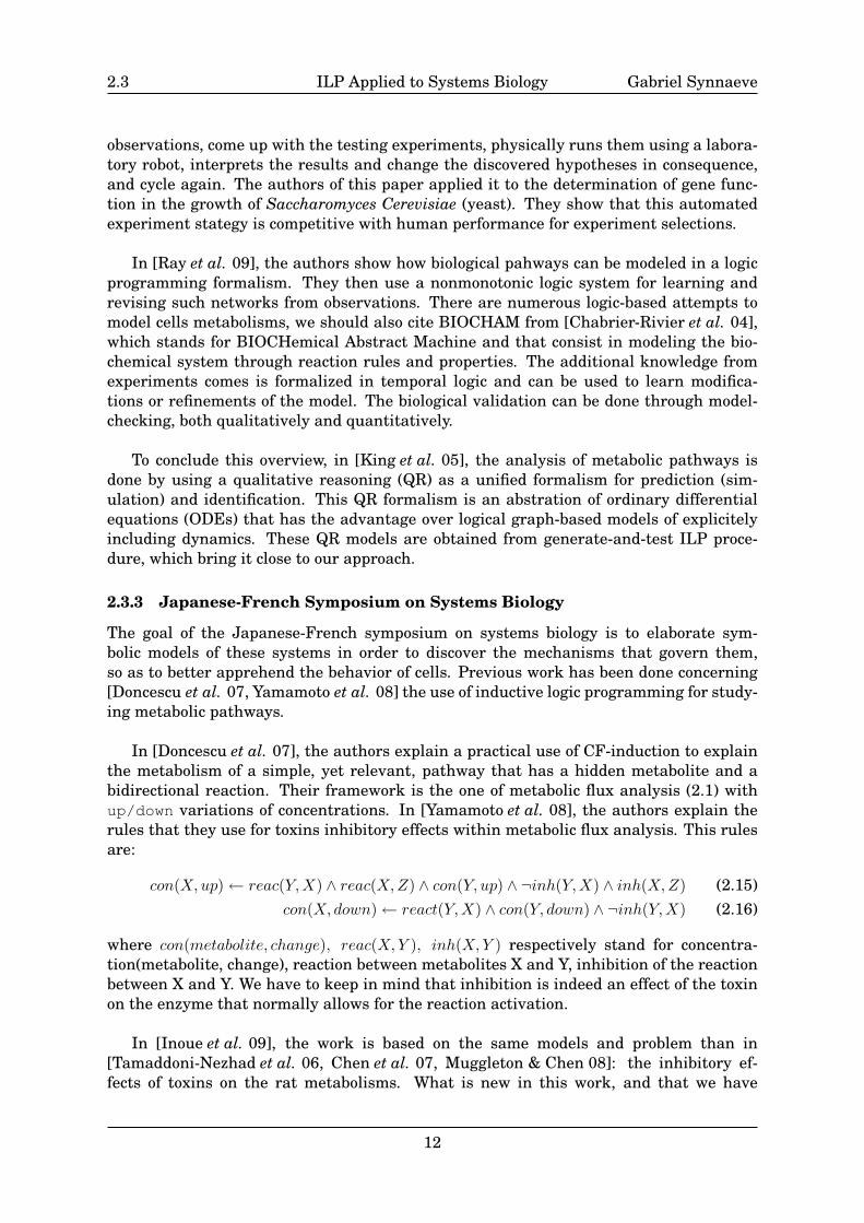
successfully used in the current one, is that it describes a method to rank hypotheseswith the help of BDD-EM [Ishihata et al. 08]. That is also in this paper that is mentionedfor the first time the full system for hypothesis finding, described in Fig.4, that we willbase our work on.
Experiments
Logically possible
hypotheses
Databases
Hypotheses Generator(SOLAR)
Hypotheses Evaluator (BDD-EM)
Background knowledge
Observations
Most probable hypotheses
Figure 4: Current biological hypothesis-finding system as explained in [Inoue et al. 09]
13
3.1 ILP Applied to Systems Biology Gabriel Synnaeve
3 Discrete Levels and Kinetic Modeling of Reactions
The kinetic model that will be presented in the following allows for the study of metabolicflux analysis by handling not only qualitative results (like changes of concentration of ametabolite between to instants) but quantitative values. For that, we clusterize contin-uous concentrations of metabolites over time into discrete levels and discrete timesteps.Then (4.3), we applied it on an inverse problem: given the measured concentrations ofsome metabolites in steady state, we compute the concentrations of metabolites beforethe dynamic transition from the perturbation that cause a pulse of glucose to this steadystate thanks to the kinetic modeling.
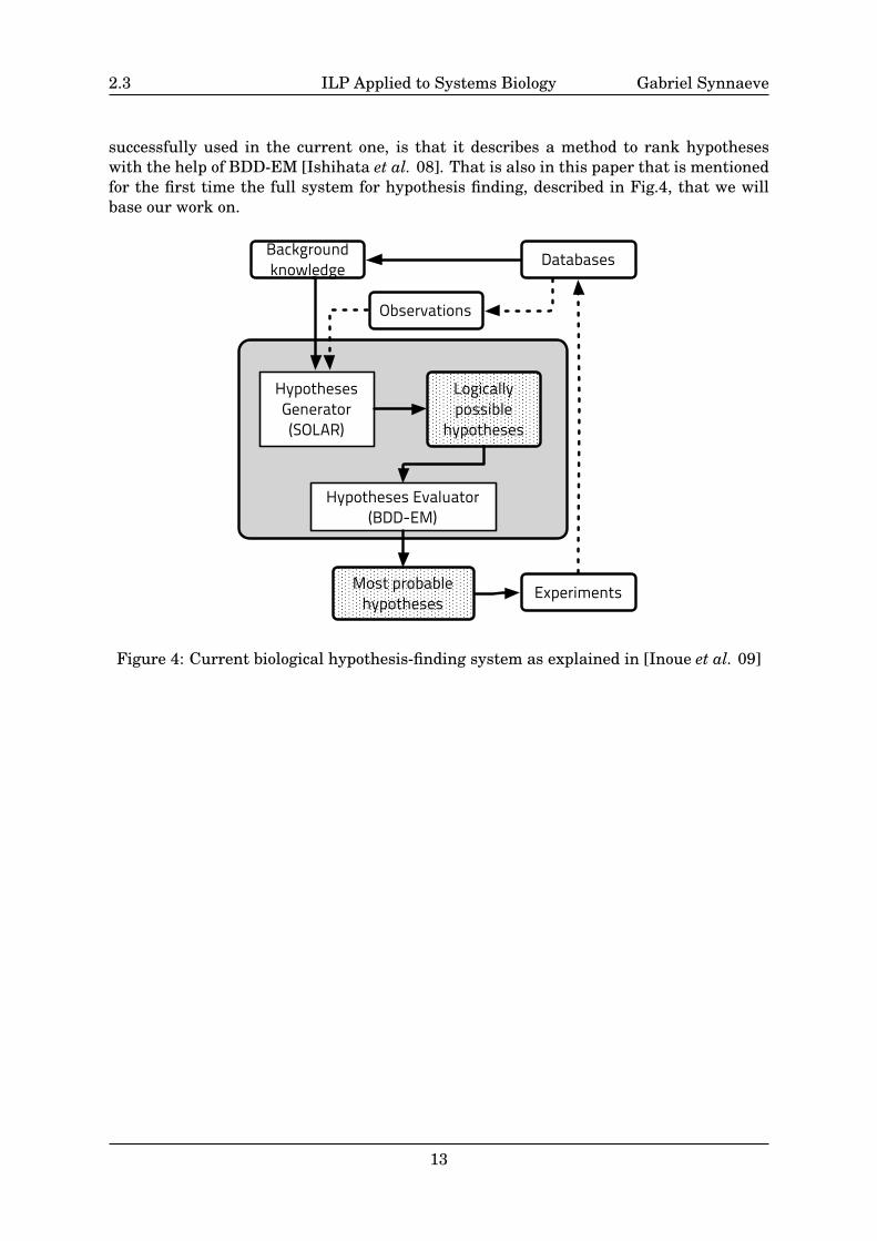
3.1 Precision – Generality trade-off
Generalization
Learning
Complexity of the Hypothesis space
Errors
currently
evolution
Figure 5: Variations of the learning and generalization errors in function of the complexityof the hypothesis space. The “evolution” arrow show where we are heading by discretizingthe time series more finely.
We are dealing with the classic problem of machine learning: given some samplesdata as input, could we learn hypotheses that describe this data in terms of importantproperties, for us to be able to predict the class (or what will happen) when we are given anew sample (an event occurs). This is also the way we, as human being, learn our lessons,make hypotheses, conclusions, and even learn to walk. Let X be the samples space andH be the hypotheses space. These spaces are generated respectively by LX , language ofthe samples, and by LH, language of the hypotheses. The task of machine learning is tofind a function X → H that associate the x ∈ X with corresponding classes hi ∈ H. Theproblem is that the x can be differing from each others by very tiny differences in theirfeatures. Which features are the most important for LH? If we try and make a machinethat learns by taking all the features into account, that is equivalent to have LX = LHand learning is simply copying the values of the features. When a new x will be given tothis machine, it will be unable to differentiate that sample from the others, in fact: everysample will be a special case.
14
3.2 ILP Applied to Systems Biology Gabriel Synnaeve
H(↓,↑)
H(⇓,↓,=,↑,⇑)
Samples space Hypothesis spaces
H(∞)
Figure 6: Trade-off between the ability to describe the samples space given the complexityof the hypothesis space
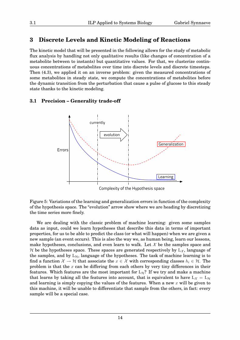
There is a recurrent problem in machine learning: the learning error is decreasingwhen the dimension of the hypotheses space is growing but the generalization errorbegins growing after some point as seen in Fig.5. As stated above, if the complexityof the hypotheses space is too big, the hypotheses will all be special cases. There arenumerous of possible metaphors for explaining machine learning, one of them that isnear the reality is that machine learning is like a data compression task: if the dictionaryof possible features (LH) is too small, there will be a lot of loss in the process andthe learning error will be big. If you specialise it too much, you will lose robustness(predictive power) and each compressed data input will be so precise that it will look likeneither of the others. That’s the strong argument in favor or Occam’s razor: “entitiesshould not be multiplied unnecessarily”, meaning that if one has to choose between twohypotheses, the best choice should be the shorter (in terms of use of LH) one.
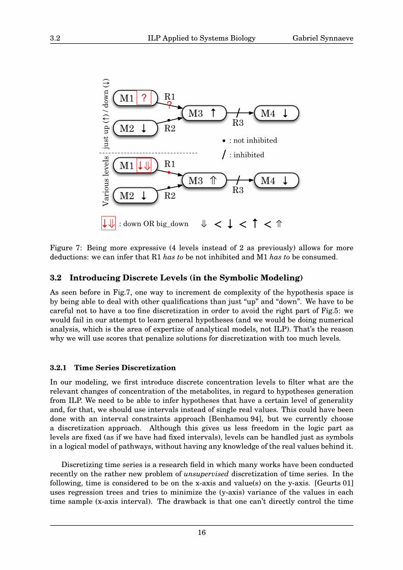
In regard to the previous results, it seemed that the limitations are due to a too smallLH with only up and down for the concentrations of metabolites. It doesn’t allow us tohave enough discrimination power between the samples (hypotheses are too simple) asshowed in Fig.6. We hope to have a better (more accurate, yet still robust) predictivepower by increasing the expressivity of the hypotheses (Fig.6). For example, if we work asin [Tamaddoni-Nezhad et al. 06, Inoue et al. 09], trying to analyze the inhibitory effect oftoxins on metabolisms based on NMR measurements on rats: up / down correspondhere to the differences between an experiment without toxins and one with an injec-tion of toxins. If we have a piece of pathway as in Fig.7 and use the same rules as in[Yamamoto et al. 08], we are unable to infer if Reaction 1 (R1) is inhibited or not with justup / down. Now if we had a finer discretization of the values and that we found thatMetabolite 3 (M3) has a big increase of concentration between the two experiments, butthat M2 has only a low decrease: we can infer that the consumption (transformation) ofM2 alone is not enough to account for M3 increase, and thus M1 should also be consumedand R1 is not inhibited.
15
3.2 ILP Applied to Systems Biology Gabriel Synnaeve
M1
M3
M2
M4/R2 R3
R1?•
⇓ < ↓ < ↑ < ⇑
M1
M3
M2
M4/R2 R3
R1
•
just
up
(↑)
/ dow
n (↓
)V
ario
us
leve
ls↑
↓
?
↓ •↓
⇑⇓
↓⇓ : down OR big_down
↓
↓
•/
: not inhibited
: inhibited
Figure 7: Being more expressive (4 levels instead of 2 as previously) allows for moredeductions: we can infer that R1 has to be not inhibited and M1 has to be consumed.
3.2 Introducing Discrete Levels (in the Symbolic Modeling)
As seen before in Fig.7, one way to increment de complexity of the hypothesis space isby being able to deal with other qualifications than just “up” and “down”. We have to becareful not to have a too fine discretization in order to avoid the right part of Fig.5: wewould fail in our attempt to learn general hypotheses (and we would be doing numericalanalysis, which is the area of expertize of analytical models, not ILP). That’s the reasonwhy we will use scores that penalize solutions for discretization with too much levels.
3.2.1 Time Series Discretization
In our modeling, we first introduce discrete concentration levels to filter what are therelevant changes of concentration of the metabolites, in regard to hypotheses generationfrom ILP. We need to be able to infer hypotheses that have a certain level of generalityand, for that, we should use intervals instead of single real values. This could have beendone with an interval constraints approach [Benhamou 94], but we currently choosea discretization approach. Although this gives us less freedom in the logic part aslevels are fixed (as if we have had fixed intervals), levels can be handled just as symbolsin a logical model of pathways, without having any knowledge of the real values behind it.
Discretizing time series is a research field in which many works have been conductedrecently on the rather new problem of unsupervised discretization of time series. In thefollowing, time is considered to be on the x-axis and value(s) on the y-axis. [Geurts 01]uses regression trees and tries to minimize the (y-axis) variance of the values in eachtime sample (x-axis interval). The drawback is that one can’t directly control the time
16
3.3 ILP Applied to Systems Biology Gabriel Synnaeve
sampling (nor the values, but this is closer to what we want with an unsuppervised clus-tering). [Keogh et al. 05] have developed “Symbolic Aggregate approXimation” (SAX) thatis built on piecewise aggregate approximation and makes a normality assumption on mea-sured values. In [Lin et al. 07], the authors showed the theoretical validity of SAX andwe considered using it. However, we didn’t see an easy way of dealing with our variousand distant (in y-axis mean) time series because of the normality assumption: we shouldhave one Gaussian for each time-series. [Morchen et al. 05] proposed the Persist algo-rithm, that is really noise-resistant. But more of that, we have been interested in theirexhaustive comparison of the quality of discretized sequences resulting from Persist, SAXand continuous hidden Markov models (CHMMs).
3.2.2 Our approach
In the end, both the facts that we had little to no noise1 in our experimental time-seriesand that we wanted to discretize our concentrations time-series all at once (with the samelevels) lead us to try and develop our own discretization method, adapted to (and takingbenefit of) the particularities of our data. Our practical problem is that we want to have astatistically relevant (unsupervised) discretization for N metabolites concentrations overtime. We also have to discretize the values of Km (Michaelis-Menten constants), for eachreaction, with the same levels.
For that purpose, we have chosen to use a probabilistic model, used in speech recog-nition and time-series analysis: continuous hidden Markov model (HMMs) [Rabiner 89].We can therefore compute an appropriate number of levels (that was 3 for the experi-ment with Escherichia Coli , 9 for the one with Saccharomyces Cerevisiae ) in regardto a Bayesian score such as Bayesian Information Criterion (BIC) [Schwarz 78] or asthe Cheeseman-Stutz score [Cheeseman & Stutz 95] or as the variational free energy.This process can be achieved through maximum likelihood estimation or maximum aposteriori estimation [Gauvain & Lee 94] or through a variational Bayesian method[Beal 03, Ji et al. 06], respectively. There are more details in the implementation partbeginning page 21.
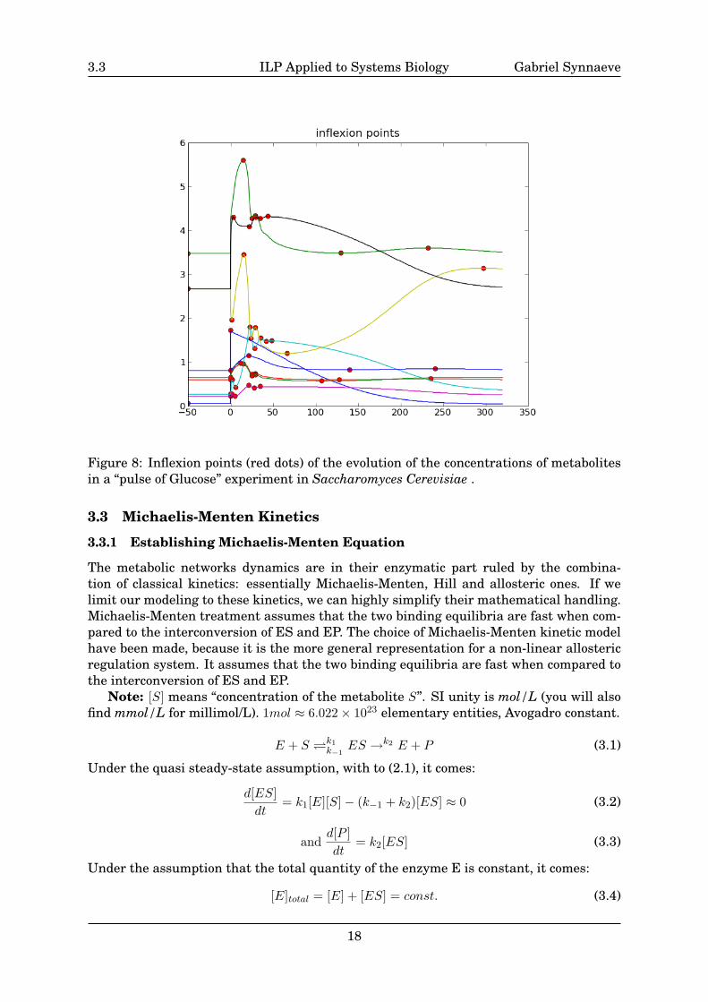
Whereas the results of CHMMs discretization are relevant and already usable. Wehave also begun working on another discretization method that heavily uses the fact thatwe have almost no noise. One can (and is obliged to) apply a filtering as Savitzky-Golay[Savitzky & Golay 64] filtering beforehand if the data is noisy (see Fig.21 page 43). Thechoice of Savitzky-Golay filtering has been made as it keeps the amplitude of the timeseries (the maximum values) and it is particularly adapted to experimental data fromchemistry [Savitzky & Golay 64]. The changes of tendencies of the concentration time-series seem important to be able to infer the cause-consequences relations with the in-ducted logic rules. With respect to this assumption, the inflexion points (see Fig.8) ofthe time series are central in this discretization approach. We use them as the seeds ofy-values clusters as well as sampling stops for the time-sampling. We should now imple-ment statistical tests to merge (prune) some levels (y-axis) and sampling stops (x-axis).
1Indeed, Andrei Doncescu provided a simulator that enables us to get very clean signals. Even withoutthat, the signal/noise ratio of experimental data would allow us to smooth is efficiently beforehand.
17
3.3 ILP Applied to Systems Biology Gabriel Synnaeve
Figure 8: Inflexion points (red dots) of the evolution of the concentrations of metabolitesin a “pulse of Glucose” experiment in Saccharomyces Cerevisiae .
3.3 Michaelis-Menten Kinetics
3.3.1 Establishing Michaelis-Menten Equation
The metabolic networks dynamics are in their enzymatic part ruled by the combina-tion of classical kinetics: essentially Michaelis-Menten, Hill and allosteric ones. If welimit our modeling to these kinetics, we can highly simplify their mathematical handling.Michaelis-Menten treatment assumes that the two binding equilibria are fast when com-pared to the interconversion of ES and EP. The choice of Michaelis-Menten kinetic modelhave been made, because it is the more general representation for a non-linear allostericregulation system. It assumes that the two binding equilibria are fast when compared tothe interconversion of ES and EP.
Note: [S] means “concentration of the metabolite S”. SI unity is mol/L (you will alsofind mmol/L for millimol/L). 1mol ≈ 6.022× 10²³ elementary entities, Avogadro constant.
E + S k1k−1
ES →k2 E + P (3.1)
Under the quasi steady-state assumption, with to (2.1), it comes:
d[ES]dt
= k1[E][S]− (k−1 + k2)[ES] ≈ 0 (3.2)
andd[P ]dt
= k2[ES] (3.3)
Under the assumption that the total quantity of the enzyme E is constant, it comes:
[E]total = [E] + [ES] = const. (3.4)
18
3.3 ILP Applied to Systems Biology Gabriel Synnaeve
(3.4) into (3.2) gives:
k1[S]([E]total − [ES]) − (k−1 + k2)[ES] = 0 (3.5)
[S][E]total = [S][ES] + [ES](k−1 + k2
k1) (3.6)
let KM =k−1 + k2
k1(3.7)
=⇒ [ES] =[S][E]totalKM + [S]
(3.8)
by replacing [ES] in (3.3) and with the maximum velocity Vm = k2[E]total, it comes:
Michaelis−Menten equation :d[P ]dt
= Vm[S]
[S] +Km(3.9)
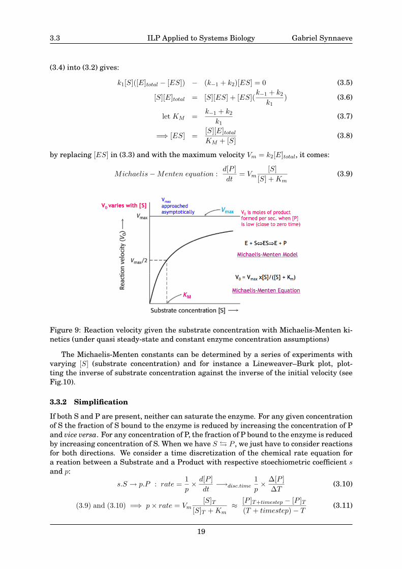
Figure 9: Reaction velocity given the substrate concentration with Michaelis-Menten ki-netics (under quasi steady-state and constant enzyme concentration assumptions)
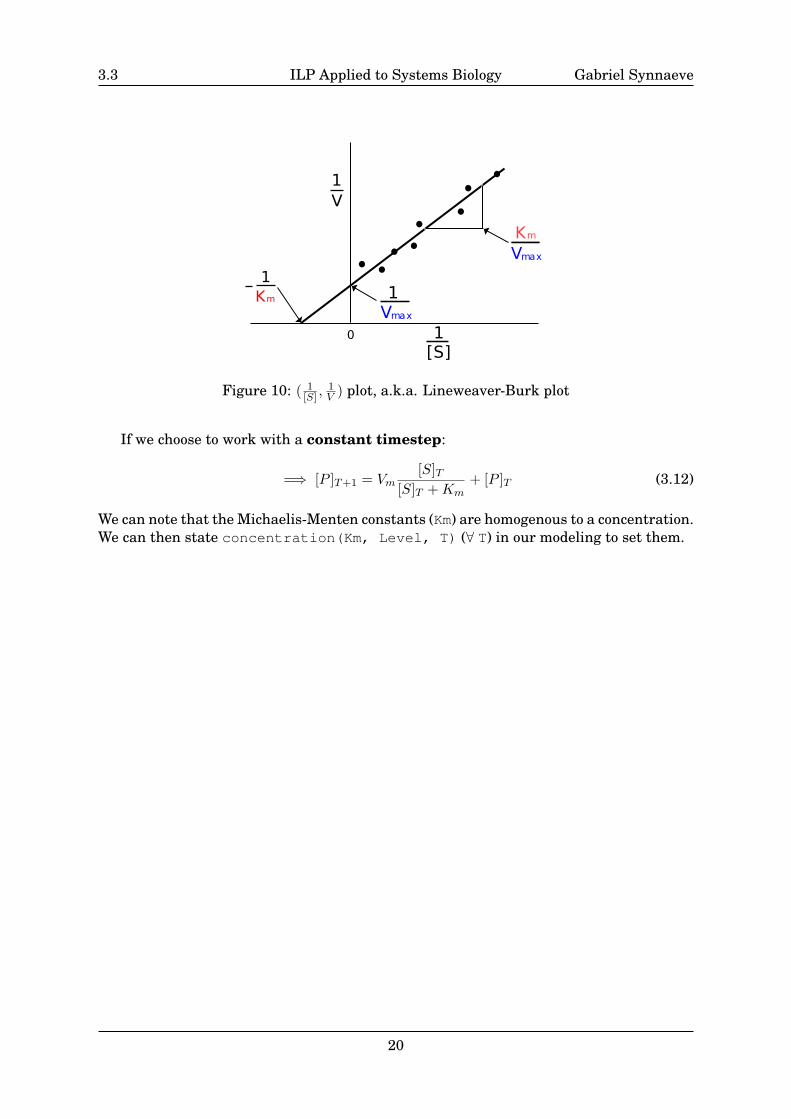
The Michaelis-Menten constants can be determined by a series of experiments withvarying [S] (substrate concentration) and for instance a Lineweaver–Burk plot, plot-ting the inverse of substrate concentration against the inverse of the initial velocity (seeFig.10).
3.3.2 Simplification
If both S and P are present, neither can saturate the enzyme. For any given concentrationof S the fraction of S bound to the enzyme is reduced by increasing the concentration of Pand vice versa. For any concentration of P, the fraction of P bound to the enzyme is reducedby increasing concentration of S. When we have S � P , we just have to consider reactionsfor both directions. We consider a time discretization of the chemical rate equation fora reation between a Substrate and a Product with respective stoechiometric coefficient sand p:
s.S → p.P : rate =1p× d[P ]
dt−→disc.time
1p× ∆[P ]
∆T(3.10)
(3.9) and (3.10) =⇒ p× rate = Vm[S]T
[S]T +Km≈
[P ]T+timestep − [P ]T(T + timestep)− T
(3.11)
19
3.3 ILP Applied to Systems Biology Gabriel Synnaeve
1V
[S]1
K1m
V1max
Km
Vmax
0
Figure 10: ( 1[S] ,
1V ) plot, a.k.a. Lineweaver-Burk plot
If we choose to work with a constant timestep:
=⇒ [P ]T+1 = Vm[S]T
[S]T +Km+ [P ]T (3.12)
We can note that the Michaelis-Menten constants (Km) are homogenous to a concentration.We can then state concentration(Km, Level, T) (∀ T) in our modeling to set them.
20
4.2 ILP Applied to Systems Biology Gabriel Synnaeve
4 Implementations and Results
We have been developping an automated framework to deal with different real worldpathways and experiments. It is currently composed of two tools:
• kegg2symb: this is a program that transforms metabolic pathways from the KEGGonline database into symbolic relational models by querying KEGG’s API (see Fig.23page 44 in Appendix).
• The combination of an implementation of continuous HMMs [Gauvain & Lee 94,Ji et al. 06] with py-tsdisc, a Python automating wrapper that takes time-seriesof concentrations of metabolites and output the corresponding symbolic predicatesconcentration(metabolite, level, time).
Both are under heavy developpement but already avaible for downloading and usethrough their working repository2 under the free BSD/MIT-Python licenses.
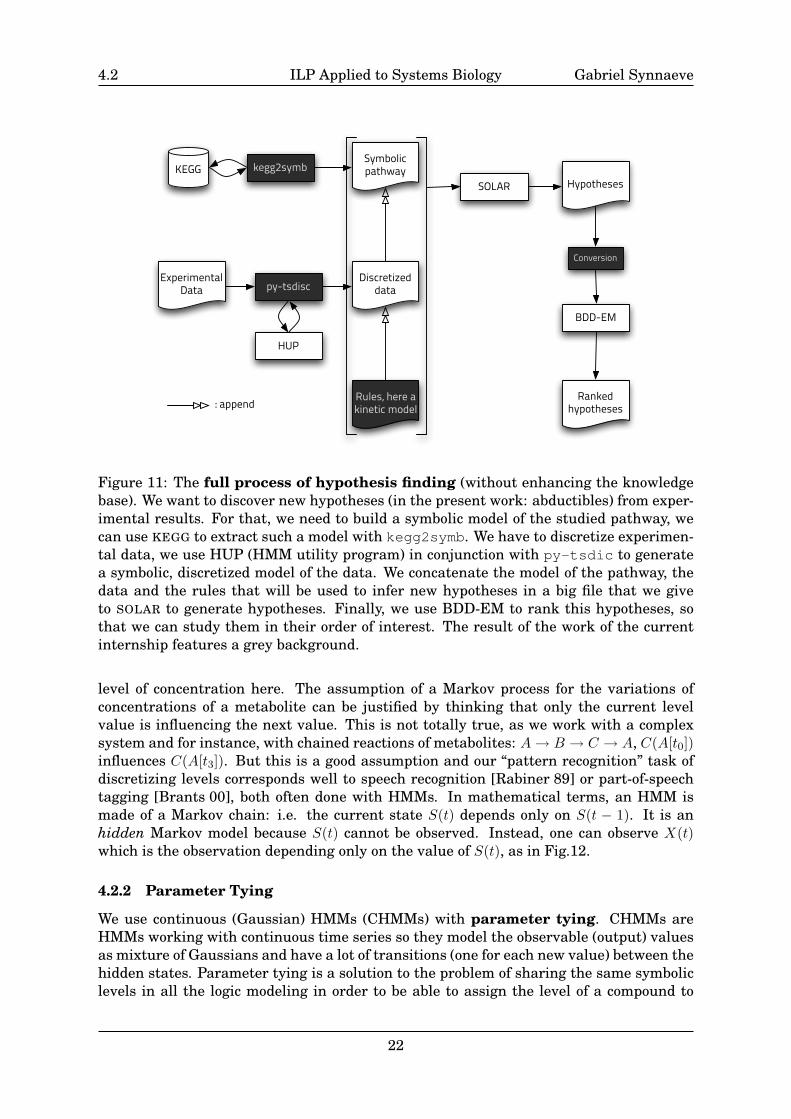
Along with that, we used SOLAR [Nabeshima et al. 03] for the hypothesis finding partand BDD-EM [Ishihata et al. 08] for ranking these hypotheses. You can see the wholepath of the data, from experimental results and KEGG database to the ranked hypothesesin figure 11 page 22. The “new” parts (this work) are the one with a grey background.
4.1 kegg2symb: Automatic Conversion of Pathways
This program generates a symbolic model with the name of a pathway from KEGG.http://www.genome.jp/dbget-bin/show_pathway?sce00010 is described in ftp://ftp.
genome.jp/pub/kegg/xml/organisms/sce/sce00010.xml.The default behavior is to parse the XML describing the map and to output the reac-
tion nodes. As all that contains the XML are IDs, it has the options:
• offline: builds the reactions with KEGG’s {enzyme:id} and {metabolite:id} with onereaction predicate per enzyme.
• genes: reactions with genes that have to be activated to produce such a protein, andmetabolites names (from KEGG’s API). One reaction predicate per gene.
• convert (default): reactions with metabolites and enzymes names (from KEGG’s API)with one reaction predicate per enzyme.
We think that this is interesting to automate such uses of existing databases to be able tobuild large models quickly and to be able to persue our automated knowledge discoveryprocess.
4.2 Discrete Levels
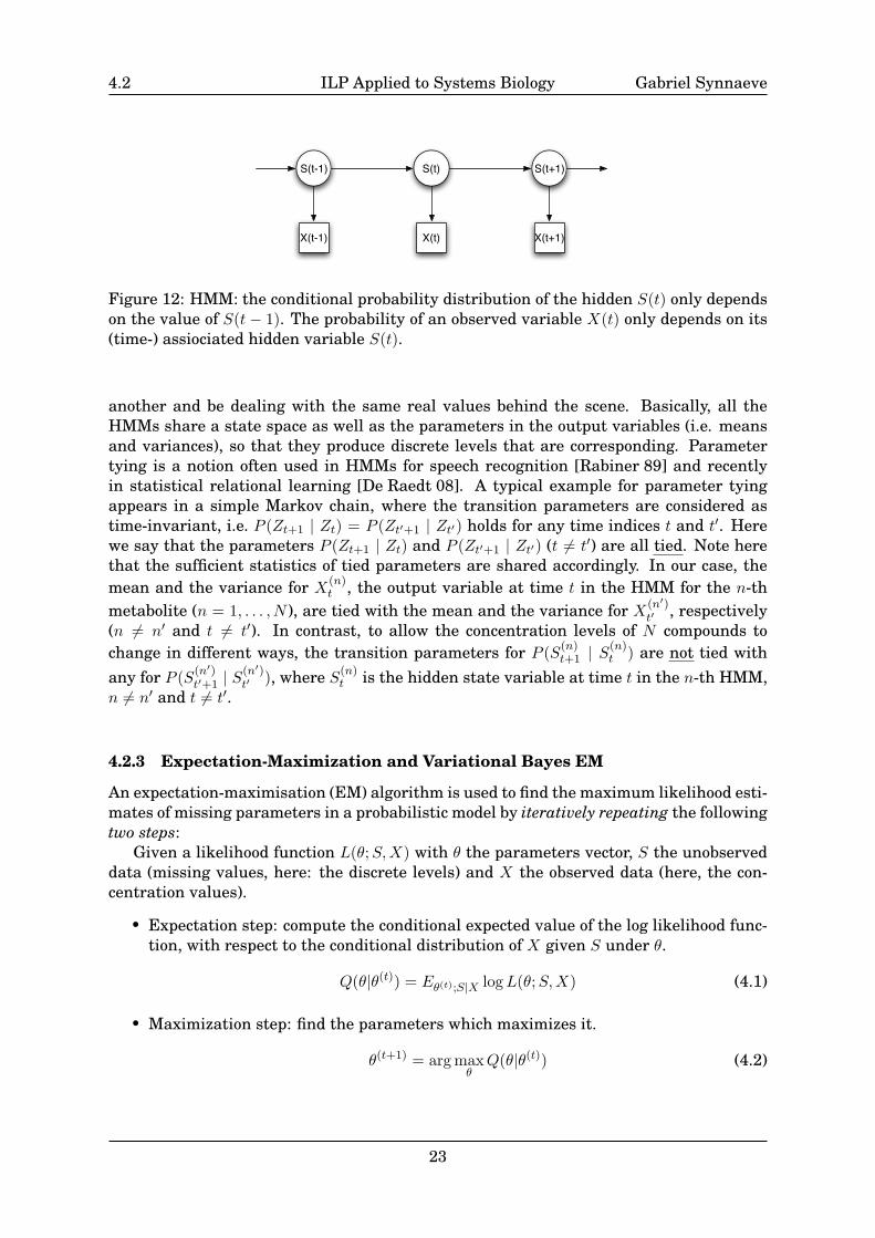
4.2.1 Hidden Markov Models
An hidden Markov model (HMM) is a statistical model in which the system being modeledis assumed to be a Markov process with unobserved state: the corresponding discrete
2kegg2symb: http://github.com/SnippyHolloW/kegg2symb/tree/master from Gabriel SynnaeveHUP: http://sato-www.cs.titech.ac.jp/kameya/hup4d/ from Yoshitaka Kameyapy-tsdisc: http://github.com/SnippyHolloW/py-tsdisc/tree/master from Gabriel Synnaeve
21
4.2 ILP Applied to Systems Biology Gabriel Synnaeve
KEGG
ExperimentalData
kegg2symbSymbolicpathway
py-tsdisc
HUP
SOLAR
Discretizeddata
Rules, here akinetic model
BDD-EM
Hypotheses
Rankedhypotheses
Conversion
: append
Figure 11: The full process of hypothesis finding (without enhancing the knowledgebase). We want to discover new hypotheses (in the present work: abductibles) from exper-imental results. For that, we need to build a symbolic model of the studied pathway, wecan use KEGG to extract such a model with kegg2symb. We have to discretize experimen-tal data, we use HUP (HMM utility program) in conjunction with py-tsdic to generatea symbolic, discretized model of the data. We concatenate the model of the pathway, thedata and the rules that will be used to infer new hypotheses in a big file that we giveto SOLAR to generate hypotheses. Finally, we use BDD-EM to rank this hypotheses, sothat we can study them in their order of interest. The result of the work of the currentinternship features a grey background.
level of concentration here. The assumption of a Markov process for the variations ofconcentrations of a metabolite can be justified by thinking that only the current levelvalue is influencing the next value. This is not totally true, as we work with a complexsystem and for instance, with chained reactions of metabolites: A→ B → C → A, C(A[t0])influences C(A[t3]). But this is a good assumption and our “pattern recognition” task ofdiscretizing levels corresponds well to speech recognition [Rabiner 89] or part-of-speechtagging [Brants 00], both often done with HMMs. In mathematical terms, an HMM ismade of a Markov chain: i.e. the current state S(t) depends only on S(t − 1). It is anhidden Markov model because S(t) cannot be observed. Instead, one can observe X(t)which is the observation depending only on the value of S(t), as in Fig.12.
4.2.2 Parameter Tying
We use continuous (Gaussian) HMMs (CHMMs) with parameter tying. CHMMs areHMMs working with continuous time series so they model the observable (output) valuesas mixture of Gaussians and have a lot of transitions (one for each new value) between thehidden states. Parameter tying is a solution to the problem of sharing the same symboliclevels in all the logic modeling in order to be able to assign the level of a compound to
22
4.2 ILP Applied to Systems Biology Gabriel Synnaeve
S(t-1) S(t) S(t+1)
X(t-1) X(t) X(t+1)
Figure 12: HMM: the conditional probability distribution of the hidden S(t) only dependson the value of S(t− 1). The probability of an observed variable X(t) only depends on its(time-) assiociated hidden variable S(t).
another and be dealing with the same real values behind the scene. Basically, all theHMMs share a state space as well as the parameters in the output variables (i.e. meansand variances), so that they produce discrete levels that are corresponding. Parametertying is a notion often used in HMMs for speech recognition [Rabiner 89] and recentlyin statistical relational learning [De Raedt 08]. A typical example for parameter tyingappears in a simple Markov chain, where the transition parameters are considered astime-invariant, i.e. P (Zt+1 | Zt) = P (Zt′+1 | Zt′) holds for any time indices t and t′. Herewe say that the parameters P (Zt+1 | Zt) and P (Zt′+1 | Zt′) (t 6= t′) are all tied. Note herethat the sufficient statistics of tied parameters are shared accordingly. In our case, themean and the variance for X(n)
t , the output variable at time t in the HMM for the n-thmetabolite (n = 1, . . . , N ), are tied with the mean and the variance for X(n′)
t′ , respectively(n 6= n′ and t 6= t′). In contrast, to allow the concentration levels of N compounds tochange in different ways, the transition parameters for P (S(n)
t+1 | S(n)t ) are not tied with
any for P (S(n′)t′+1 | S
(n′)t′ ), where S(n)
t is the hidden state variable at time t in the n-th HMM,n 6= n′ and t 6= t′.
4.2.3 Expectation-Maximization and Variational Bayes EM
An expectation-maximisation (EM) algorithm is used to find the maximum likelihood esti-mates of missing parameters in a probabilistic model by iteratively repeating the followingtwo steps:
Given a likelihood function L(θ;S,X) with θ the parameters vector, S the unobserveddata (missing values, here: the discrete levels) and X the observed data (here, the con-centration values).
• Expectation step: compute the conditional expected value of the log likelihood func-tion, with respect to the conditional distribution of X given S under θ.
Q(θ|θ(t)) = Eθ(t);S|X logL(θ;S,X) (4.1)
• Maximization step: find the parameters which maximizes it.
θ(t+1) = arg maxθQ(θ|θ(t)) (4.2)
23
4.2 ILP Applied to Systems Biology Gabriel Synnaeve
f(z)L(z;z1)
L(z;z0)
L(z;z2)
Figure 13: f is convex, any tangent L(z; zi) can be used as its lower bound
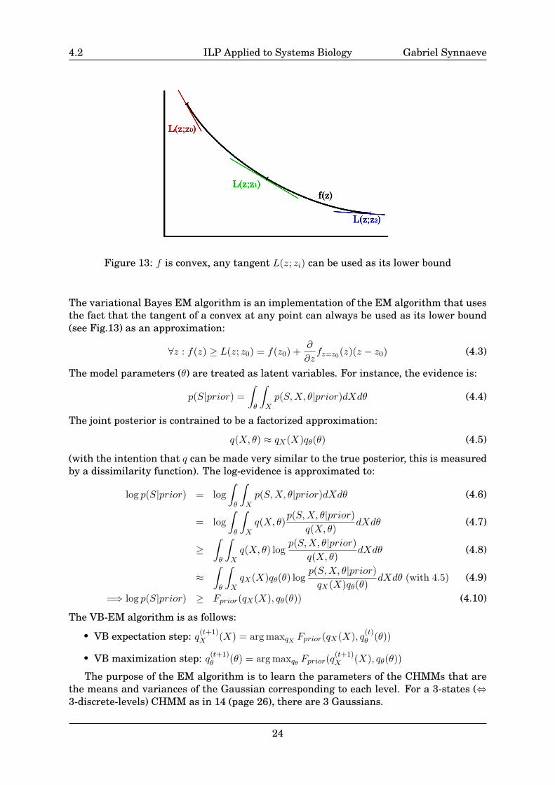
The variational Bayes EM algorithm is an implementation of the EM algorithm that usesthe fact that the tangent of a convex at any point can always be used as its lower bound(see Fig.13) as an approximation:
∀z : f(z) ≥ L(z; z0) = f(z0) +∂
∂zfz=z0(z)(z − z0) (4.3)
The model parameters (θ) are treated as latent variables. For instance, the evidence is:
p(S|prior) =∫θ
∫Xp(S,X, θ|prior)dXdθ (4.4)
The joint posterior is contrained to be a factorized approximation:
q(X, θ) ≈ qX(X)qθ(θ) (4.5)
(with the intention that q can be made very similar to the true posterior, this is measuredby a dissimilarity function). The log-evidence is approximated to:
log p(S|prior) = log∫θ
∫Xp(S,X, θ|prior)dXdθ (4.6)
= log∫θ
∫Xq(X, θ)
p(S,X, θ|prior)q(X, θ)
dXdθ (4.7)
≥∫θ
∫Xq(X, θ) log
p(S,X, θ|prior)q(X, θ)
dXdθ (4.8)
≈∫θ
∫XqX(X)qθ(θ) log
p(S,X, θ|prior)qX(X)qθ(θ)
dXdθ (with 4.5) (4.9)
=⇒ log p(S|prior) ≥ Fprior(qX(X), qθ(θ)) (4.10)
The VB-EM algorithm is as follows:
• VB expectation step: q(t+1)X (X) = arg maxqX Fprior(qX(X), q(t)
θ (θ))
• VB maximization step: q(t+1)θ (θ) = arg maxqθ Fprior(q
(t+1)X (X), qθ(θ))
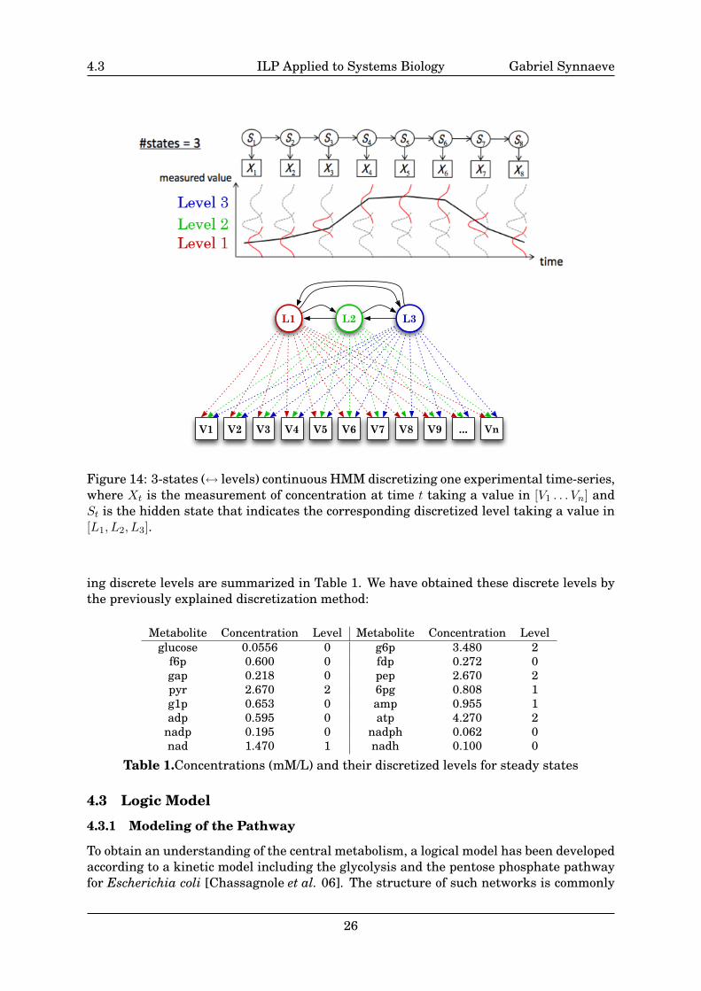
The purpose of the EM algorithm is to learn the parameters of the CHMMs that arethe means and variances of the Gaussian corresponding to each level. For a 3-states (⇔3-discrete-levels) CHMM as in 14 (page 26), there are 3 Gaussians.
24
4.2 ILP Applied to Systems Biology Gabriel Synnaeve
4.2.4 Discretization Process
The relevant discretized levels of concentration are computed through the EM algorithmwith maximum a posteriori (MAP) estimation [Gauvain & Lee 94] (Baum-Welch algo-rithm) or through the variational Bayes EM (VB-EM) [Beal 03, Ji et al. 06]. We preferthis last method as it is shown [Beal 03] that variational free energy provides a moreaccurate approximation of the marginal log-likelihood than BIC or the Cheeseman-Stutzscore. The discretization process itself simply consist in choosing with which discretelevel will be mapped some numerical value of the time series. This is done by finding themost probable states sequence in the CHMM, once the parameters are all learned andtuned. For an example, see in appendix page 44. All of this is done with the help of HMMutility program (HUP) from Yoshitaka Kameya.
We first prepare N continuous HMMs (one for each metabolite), where each statevariable takes a concentration level, and each output variable takes a measurement ofconcentration (2nd figure of Fig.14) and follows a univariate Gaussian distribution (1stfigure of Fig.14). For knowing which number of states (levels) k? is better fitting for ourset of time series (one for each metabolite), we test a range [i . . . j]. We then run VB-EM(or another EM algorithm) p times for each level and take the best outputs in regard tothe scores (see below). We need to do numerous runs because variational Bayes is anapproximate framework. We score the p CHMMs models (differing by their parameters,not the structure) of each level and take the best. We end up with (j − i) CHMMs dis-cretizing in [i..j] levels, the “better fitting” number of levels has just been computed inan unsuppervised manner by taking the only one best score among this lasting (j − i)CHMMs: this is the number of states. We can now recycle this very one CHMM and useit to find its most probable sequence (for instance with the Viterbi algorithm) that will beour discretized levels output sequence. For example, if we set p = 100 and test withinthe range k ∈ [3 . . . 15], so we run 120 ((15 − 3) × 100) times the VB-EM algorithm on theN continuous HMM with an increasing number of states (levels), from 3 to 15. At each“level-step”, we keep only the highest scoring CHMM, we end up with 12 CHMMs. Wetake the best one, let it be the 3 states (3 levels) CHMM as for our simplified EscherichiaColi model and as in Fig.14. The discretization of the time series of concentrations is themost probable sequence of this CHMM: 1-1-2-3-3-3-2-1.
Then, we use a simple round-mean aggregation of them for time-sampling. We seta maximal number of time steps and look for the better fitting width and alignmentfor equal-width time intervals. We are currently developping a different discretizationprocess (inside py-tsdisc) for time-series from molecular biology experiments that willdiscretize time and levels simultaneously but current results are already useable (seeTable 1., Fig.18 and Fig.22) and that is what we based the results presented here on.
The experimental response observations of intracellular metabolites to a pulseof glucose were measured in continuous culture employing automatic stopped flowand manual fast sampling techniques in the time-span of seconds and millisec-onds after the stimulus with glucose. The extracellular glucose, the intracellu-lar metabolites: glucose6phosphate, fructose6phosphate, fructose1-6bisphosphate, glyc-eraldehyde3phosphate, phospho-enolpyruvate, pyruvate, 6phosphate-gluconate, glu-cose1phosphate as well as the cometabolites: atp, adp, amp, nad, nadh, nadp, nadph weremeasured using enzymatic methods or High Performance Liquid Chromatography. Allthe measured steady-state concentrations of the E.Coli experiment and their correspond-
25
4.3 ILP Applied to Systems Biology Gabriel Synnaeve
L1 L2 L3
V1 V2 V3 V4 V5 V6 V7 V8 V9 ... Vn
Figure 14: 3-states (↔ levels) continuous HMM discretizing one experimental time-series,where Xt is the measurement of concentration at time t taking a value in [V1 . . . Vn] andSt is the hidden state that indicates the corresponding discretized level taking a value in[L1, L2, L3].
ing discrete levels are summarized in Table 1. We have obtained these discrete levels bythe previously explained discretization method:
Metabolite Concentration Level Metabolite Concentration Levelglucose 0.0556 0 g6p 3.480 2
f6p 0.600 0 fdp 0.272 0gap 0.218 0 pep 2.670 2pyr 2.670 2 6pg 0.808 1g1p 0.653 0 amp 0.955 1adp 0.595 0 atp 4.270 2
nadp 0.195 0 nadph 0.062 0nad 1.470 1 nadh 0.100 0
Table 1.Concentrations (mM/L) and their discretized levels for steady states
4.3 Logic Model
4.3.1 Modeling of the Pathway
To obtain an understanding of the central metabolism, a logical model has been developedaccording to a kinetic model including the glycolysis and the pentose phosphate pathwayfor Escherichia coli [Chassagnole et al. 06]. The structure of such networks is commonly
26
4.3 ILP Applied to Systems Biology Gabriel Synnaeve
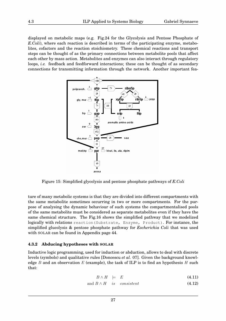
displayed on metabolic maps (e.g. Fig.24 for the Glycolysis and Pentose Phosphate ofE.Coli), where each reaction is described in terms of the participating enzyme, metabo-lites, cofactors and the reaction stoichiometry. These chemical reactions and transportsteps can be thought of as the primary connections between metabolite pools that affecteach other by mass action. Metabolites and enzymes can also interact through regulatoryloops, i.e. feedback and feedforward interactions; these can be thought of as secondaryconnections for transmitting information through the network. Another important fea-
Figure 15: Simplified glycolysis and pentose phosphate pathways of E.Coli
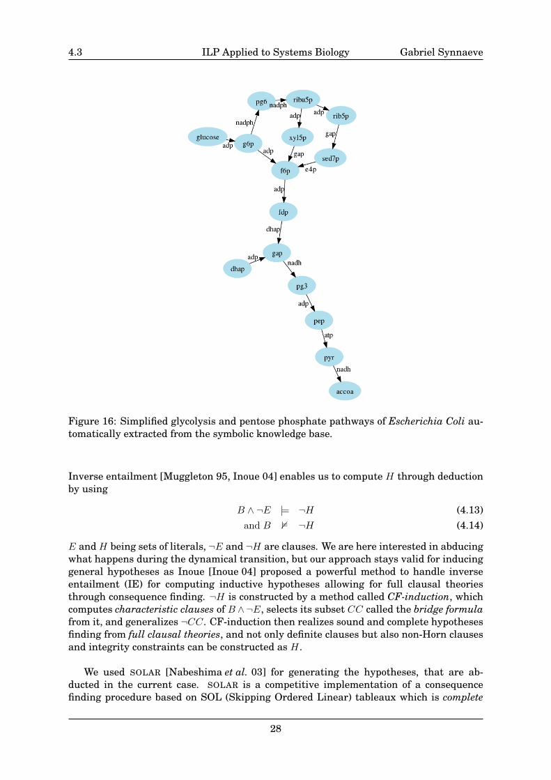
ture of many metabolic systems is that they are divided into different compartments withthe same metabolite sometimes occurring in two or more compartments. For the pur-pose of analysing the dynamic behaviour of such systems the compartmentalised poolsof the same metabolite must be considered as separate metabolites even if they have thesame chemical structure. The Fig.16 shows the simplified pathway that we modelizedlogically with relations reaction(Substrate, Enzyme, Product). For instance, thesimplified glucolysis & pentose phosphate pathway for Escherichia Coli that was usedwith SOLAR can be found in Appendix page 44.
4.3.2 Abducing hypotheses with SOLAR
Inductive logic programming, used for induction or abduction, allows to deal with discretelevels (symbols) and qualitative rules [Doncescu et al. 07]. Given the background knowl-edge B and an observation E (example), the task of ILP is to find an hypothesis H suchthat:
B ∧H |= E (4.11)and B ∧H is consistent (4.12)
27
4.3 ILP Applied to Systems Biology Gabriel Synnaeve
Figure 16: Simplified glycolysis and pentose phosphate pathways of Escherichia Coli au-tomatically extracted from the symbolic knowledge base.
Inverse entailment [Muggleton 95, Inoue 04] enables us to compute H through deductionby using
B ∧ ¬E |= ¬H (4.13)and B 2 ¬H (4.14)
E and H being sets of literals, ¬E and ¬H are clauses. We are here interested in abducingwhat happens during the dynamical transition, but our approach stays valid for inducinggeneral hypotheses as Inoue [Inoue 04] proposed a powerful method to handle inverseentailment (IE) for computing inductive hypotheses allowing for full clausal theoriesthrough consequence finding. ¬H is constructed by a method called CF-induction, whichcomputes characteristic clauses of B ∧¬E, selects its subset CC called the bridge formulafrom it, and generalizes ¬CC. CF-induction then realizes sound and complete hypothesesfinding from full clausal theories, and not only definite clauses but also non-Horn clausesand integrity constraints can be constructed as H.
We used SOLAR [Nabeshima et al. 03] for generating the hypotheses, that are ab-ducted in the current case. SOLAR is a competitive implementation of a consequencefinding procedure based on SOL (Skipping Ordered Linear) tableaux which is complete
28
4.3 ILP Applied to Systems Biology Gabriel Synnaeve
for finding minimal explanations. SOLAR is a part of CF-induction and can be used as anabductive procedure to infer an hypothesis H in the form of a set of literals. It can alsooutput all the proofs (iterations) for each hypothesis of the returned set of hypotheses. Forabducing hypotheses through IE, we need to input B ∧ ¬E to deduce ¬H. Thus, all ourobservations [e1 ∧ · · · ∧ en] will be inputed in SOLAR as a “top clause” [¬e1, . . . ,¬en] usedtogether with B to deduce ¬H, the output of SOLAR . As the output of SOLAR is a con-junction of disjunctions, we have to negate it to have a disjunction of conjunctions: eachconjunction being an hypothesis H ∈ H.
4.3.3 Kinetic Modeling
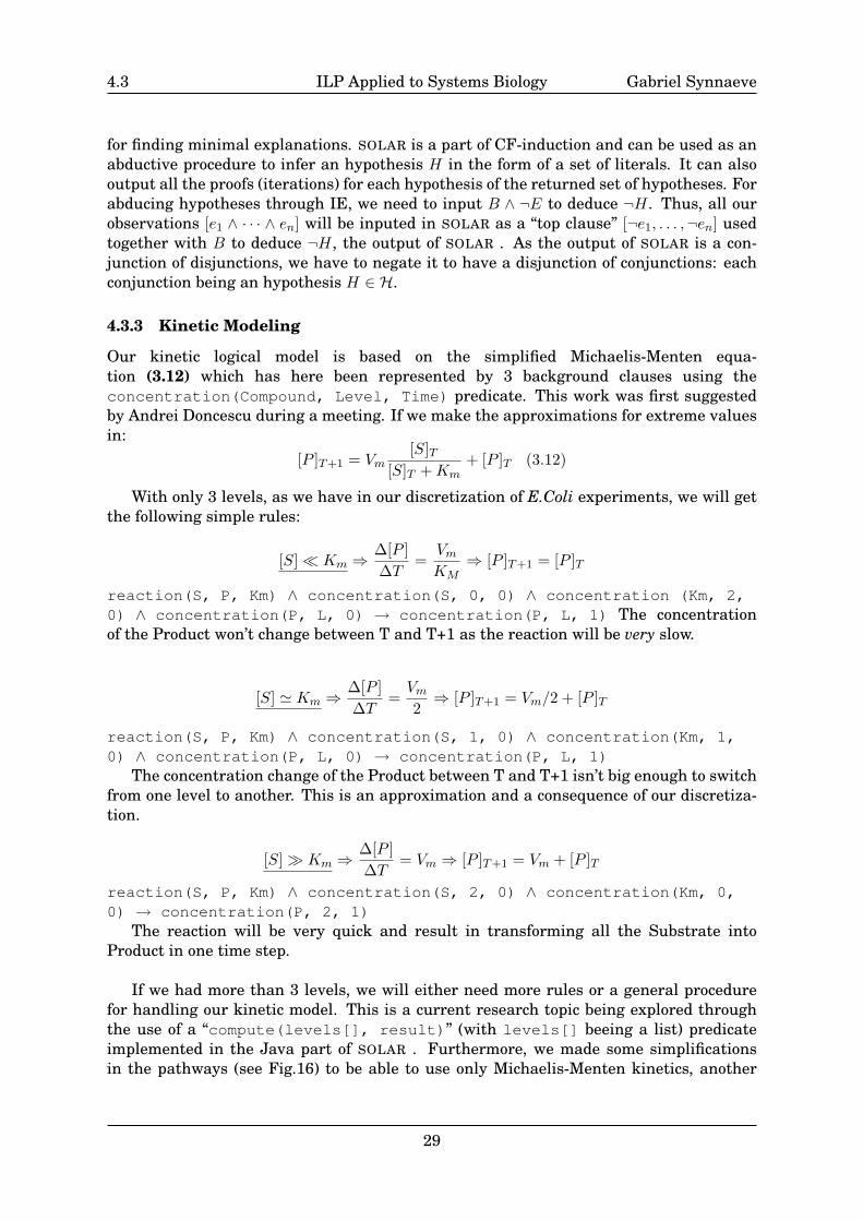
Our kinetic logical model is based on the simplified Michaelis-Menten equa-tion (3.12) which has here been represented by 3 background clauses using theconcentration(Compound, Level, Time) predicate. This work was first suggestedby Andrei Doncescu during a meeting. If we make the approximations for extreme valuesin:
[P ]T+1 = Vm[S]T
[S]T +Km+ [P ]T (3.12)
With only 3 levels, as we have in our discretization of E.Coli experiments, we will getthe following simple rules:
[S]� Km ⇒∆[P ]∆T
=VmKM
⇒ [P ]T+1 = [P ]T
reaction(S, P, Km) ∧ concentration(S, 0, 0) ∧ concentration (Km, 2,0) ∧ concentration(P, L, 0) → concentration(P, L, 1) The concentrationof the Product won’t change between T and T+1 as the reaction will be very slow.
[S] ' Km ⇒∆[P ]∆T
=Vm2⇒ [P ]T+1 = Vm/2 + [P ]T
reaction(S, P, Km) ∧ concentration(S, 1, 0) ∧ concentration(Km, 1,0) ∧ concentration(P, L, 0) → concentration(P, L, 1)
The concentration change of the Product between T and T+1 isn’t big enough to switchfrom one level to another. This is an approximation and a consequence of our discretiza-tion.
[S]� Km ⇒∆[P ]∆T
= Vm ⇒ [P ]T+1 = Vm + [P ]T
reaction(S, P, Km) ∧ concentration(S, 2, 0) ∧ concentration(Km, 0,0) → concentration(P, 2, 1)
The reaction will be very quick and result in transforming all the Substrate intoProduct in one time step.
If we had more than 3 levels, we will either need more rules or a general procedurefor handling our kinetic model. This is a current research topic being explored throughthe use of a “compute(levels[], result)” (with levels[] beeing a list) predicateimplemented in the Java part of SOLAR . Furthermore, we made some simplificationsin the pathways (see Fig.16) to be able to use only Michaelis-Menten kinetics, another
29
4.4 ILP Applied to Systems Biology Gabriel Synnaeve
research topic is to extend our modeling to other type of reactions. These rules are subjectto changes for others purposes.
We also added constraints about the unicity of levels at a given time to reduce thenumber of hypotheses while keeping consistency:
• ¬concentration(S, 0, T) ∨ ¬concentration(S, 1, T)
• ¬concentration(S, 0, T) ∨ ¬concentration(S, 2, T)
• ¬concentration(S, 1, T) ∨ ¬concentration(S, 2, T)
4.4 Results
We chose to study the conjunction of glycolysis and pentose phosphate pathways forE.Coli. We simplified the pathway’s model: we kept 16 relevant reactions (see Fig.16) anddiscretized the 16 experimental values (see Table 1). We added the 3 Michaelis-Mentenbased rules and the 3 constraints of unicity for the levels3 . We had 15 abducibles cor-responding to the unknown concentrations of chemical compounds before the transitionto steady state. SOLAR , used for abduction, outputs 410 hypotheses that cover all thisabducibles. With such a number, picking the right hypotheses should be done in anautomated way. We also discuss here how we could improve the knowledge with the“most interesting” hypotheses.
4.4.1 Ranking the Hypotheses with BDD-EM
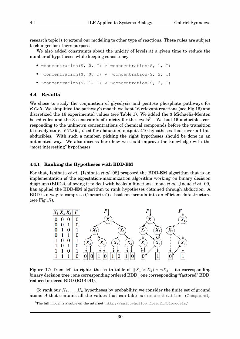
For that, Ishihata et al. [Ishihata et al. 08] proposed the BDD-EM algorithm that is animplementation of the expectation-maximization algorithm working on binary decisiondiagrams (BDDs), allowing it to deal with boolean functions. Inoue et al. [Inoue et al. 09]has applied the BDD-EM algorithm to rank hypotheses obtained through abduction. ABDD is a way to compress (“factorize”) a boolean formula into an efficient datastructure(see Fig.17).
Figure 17: from left to right: the truth table of [(X1 ∨ X2) ∧ ¬X3] ; its correspondingbinary decision tree ; one corresponding ordered BDD ; one corresponding “factored” BDD:reduced ordered BDD (ROBDD).
To rank our H1, . . . ,Hn hypotheses by probability, we consider the finite set of groundatoms A that contains all the values that can take our concentration (Compound,
3The full model is avaible on the internet: http://snippyhollow.free.fr/biomodels/
30
4.4 ILP Applied to Systems Biology Gabriel Synnaeve
Level, Time) and reaction(Substrate, Product, Km). Each of the elements ofA is a boolean variable. One of its subsets is the subset of abducibles Γ composed of allthe possible values of concentration(Compounds, Level, 0). With {Ai ∈ A | θi =P (Ai)}, we have to maximize the probability of the disjunction of hypotheses helped withthe background knowledge B: F = (H1 ∨ · · · ∨ Hn) ∧ B to set the good θ parameters (bythe BDD-EM algorithm). F can still be to big to be retained as a BDD, so an optimisationF ′ of its size is obtained through the use of the minimal proofs for B and each Hi (see[Inoue et al. 09] for more details). Then, the BDD-EM algorithm computes the probabili-ties of ground atoms in A that maximizes the probability of F ′. Finally, the probabilitiesof each hypotheses used for the ranking are computed as the products of the probabilitiesof literals appearing in each Hi.
We get 410 hypotheses in the form:H130 = concentration(glucose,0,1)∧concentration(g6p,2,1)
∧concentration(f6p,0,1)∧concentration(fdp,0,1)∧concentration(gap,0,1)∧concentration(pg3,2,0)∧concentration(adp,0,0)∧concentration(pyr,2,1)∧concentration(pg6,1,1)∧concentration(g1p,0,1)∧concentration(amp,1,1)∧concentration(adp,0,1)∧concentration(atp,2,1)∧concentration(nadp,0,1)∧concentration(nadph,0,1)∧concentration(nad,1,1)∧concentration(nadh,0,1)
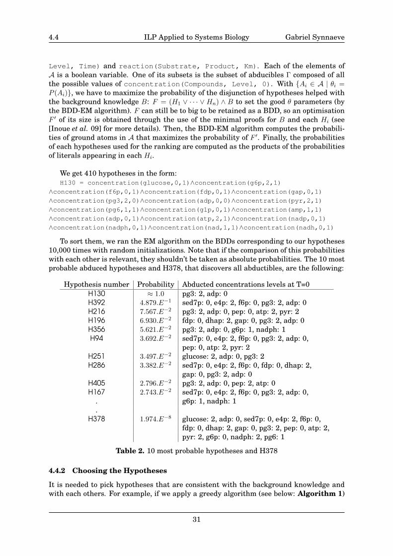
To sort them, we ran the EM algorithm on the BDDs corresponding to our hypotheses10,000 times with random initializations. Note that if the comparison of this probabilitieswith each other is relevant, they shouldn’t be taken as absolute probabilities. The 10 mostprobable abduced hypotheses and H378, that discovers all abductibles, are the following:
Hypothesis number Probability Abducted concentrations levels at T=0H130 ≈ 1.0 pg3: 2, adp: 0H392 4.879.E−1 sed7p: 0, e4p: 2, f6p: 0, pg3: 2, adp: 0H216 7.567.E−2 pg3: 2, adp: 0, pep: 0, atp: 2, pyr: 2H196 6.930.E−2 fdp: 0, dhap: 2, gap: 0, pg3: 2, adp: 0H356 5.621.E−2 pg3: 2, adp: 0, g6p: 1, nadph: 1H94 3.692.E−2 sed7p: 0, e4p: 2, f6p: 0, pg3: 2, adp: 0,
pep: 0, atp: 2, pyr: 2H251 3.497.E−2 glucose: 2, adp: 0, pg3: 2H286 3.382.E−2 sed7p: 0, e4p: 2, f6p: 0, fdp: 0, dhap: 2,
gap: 0, pg3: 2, adp: 0H405 2.796.E−2 pg3: 2, adp: 0, pep: 2, atp: 0H167 2.743.E−2 sed7p: 0, e4p: 2, f6p: 0, pg3: 2, adp: 0,
. g6p: 1, nadph: 1
.H378 1.974.E−8 glucose: 2, adp: 0, sed7p: 0, e4p: 2, f6p: 0,
fdp: 0, dhap: 2, gap: 0, pg3: 2, pep: 0, atp: 2,pyr: 2, g6p: 0, nadph: 2, pg6: 1
Table 2. 10 most probable hypotheses and H378
4.4.2 Choosing the Hypotheses
It is needed to pick hypotheses that are consistent with the background knowledge andwith each others. For example, if we apply a greedy algorithm (see below: Algorithm 1)
31
4.4 ILP Applied to Systems Biology Gabriel Synnaeve
that picks hypothesis in decreasing probability order such that the hypothesis add someknowledge and that our enhanced knowledge is still consistent to this 10 first hypotheses,we will pick H130, H392, H216, H196, H356 and H251. It will result in discovering theconcentrations at time T=0 of pg3: 2, adp: 0, sed7p: 0, e4p: 2, f6p: 0, pep: 0, atp: 2, pyr:2, fdp: 0, gap: 0, dhap: 0, g6p: 1, nadph: 1, glucose: 2. We could go further and apply it onall the hypotheses for finding values for all the abducibles.
At first, we consider the background knowledge combined with the observations as ourknowledge base. The goal of such an algorithm is to enhance (update) our knowledge basewith discovered abductibles.
Algorithm 1 An algorithm to enhance the knowledge base: most probables firstsknowledge← knowledge basesorted hypotheses← sort(hypotheses)while length(abductibles) > 0 && length(sorted hypotheses) > 0 do
tmp← sorted hypotheses.pop()if contains(tmp, abductibles) && consistent(tmp, knowledge) then
knowledge.enhance(tmp)abductibles.remove(tmp)
end ifend while
With the explicit functions length, pop (destructive), and:
• sort is a function that sorts the hypotheses by decreasing probability.
• contains is a function that returns statements of first argument contained in thesecond.
• consistent performs consistency checking of two theories and return True if they areconsistent.
• enhance adds statements that are not yet present in the considered (“self”, “this”)knowledge.
• remove deletes statements from argument present in the considered (“self”, “this”)object (could make use of contains).
4.4.3 Interpretation
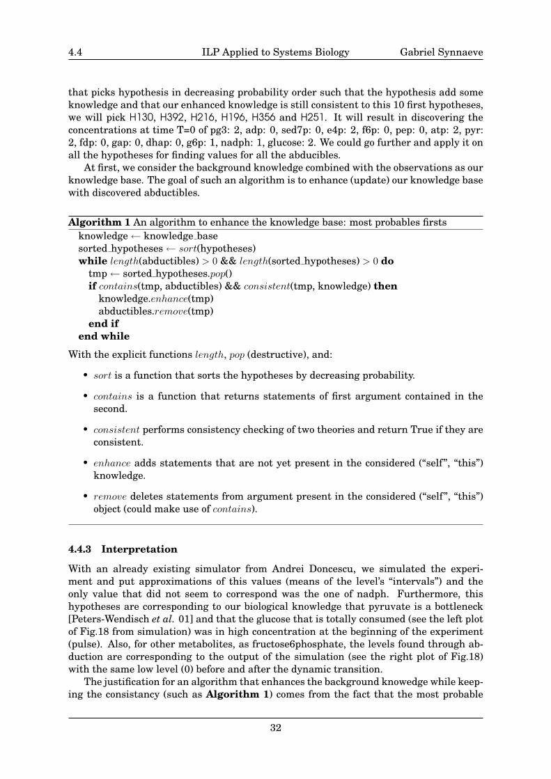
With an already existing simulator from Andrei Doncescu, we simulated the experi-ment and put approximations of this values (means of the level’s “intervals”) and theonly value that did not seem to correspond was the one of nadph. Furthermore, thishypotheses are corresponding to our biological knowledge that pyruvate is a bottleneck[Peters-Wendisch et al. 01] and that the glucose that is totally consumed (see the left plotof Fig.18 from simulation) was in high concentration at the beginning of the experiment(pulse). Also, for other metabolites, as fructose6phosphate, the levels found through ab-duction are corresponding to the output of the simulation (see the right plot of Fig.18)with the same low level (0) before and after the dynamic transition.
The justification for an algorithm that enhances the background knowedge while keep-ing the consistancy (such as Algorithm 1) comes from the fact that the most probable
32
4.4 ILP Applied to Systems Biology Gabriel Synnaeve
Figure 18: Left: Discretization in 3 levels of the concentration of glucose in the GlycolysisPathway of E.Coli after an initial pulse. Right: Simulated evolution of fructose6phosphateduring the whole experiment of pulse of glucose on E.Coli.
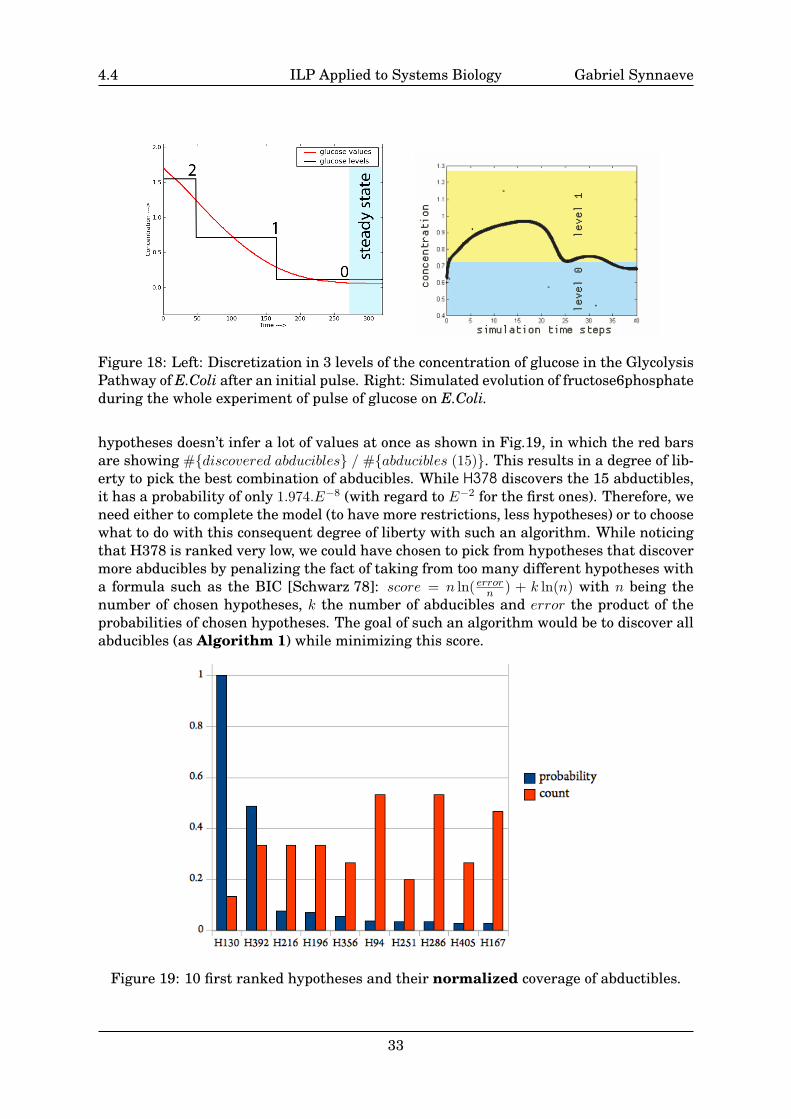
hypotheses doesn’t infer a lot of values at once as shown in Fig.19, in which the red barsare showing #{discovered abducibles} / #{abducibles (15)}. This results in a degree of lib-erty to pick the best combination of abducibles. While H378 discovers the 15 abductibles,it has a probability of only 1.974.E−8 (with regard to E−2 for the first ones). Therefore, weneed either to complete the model (to have more restrictions, less hypotheses) or to choosewhat to do with this consequent degree of liberty with such an algorithm. While noticingthat H378 is ranked very low, we could have chosen to pick from hypotheses that discovermore abducibles by penalizing the fact of taking from too many different hypotheses witha formula such as the BIC [Schwarz 78]: score = n ln( errorn ) + k ln(n) with n being thenumber of chosen hypotheses, k the number of abducibles and error the product of theprobabilities of chosen hypotheses. The goal of such an algorithm would be to discover allabducibles (as Algorithm 1) while minimizing this score.
Figure 19: 10 first ranked hypotheses and their normalized coverage of abductibles.
33
5.1 ILP Applied to Systems Biology Gabriel Synnaeve
5 Possible Extensions of this Work
5.1 Kinetic Modeling
Why is it important to have many levels ? To be able to handle the differentKm (MichaelisMenten constant): Km(ATP) = 0.4 mmol/L←→ Km(HCO−3 ) = 26 mmol/L.With M levels, for example: 1 2 3 4 5 6 7. When the need for N < M levels arises,we do a projection, for example:
small: {1, 2} ; medium: {3} ; big: {4, 5, 6, 7}
Here, if we have only the 3 previously presented rules (Michaelis-Menten specificapproximations).How ? We center medium on the discrete level of the relevant Km by doing medium(A):- level(A)==level(Km) in the context of a reaction with a substract of product A andconstant Km. This means that the discrete level that will correspond to medium for thecurrent application of the three 3-levels-based rules will be the level taken by Km. Wemade a projection.
Another way to deal with numerous levels is to change our modeling to allow forone (or many) more general(s) rule than the 3 rules showed above and resulting fromapproximations. This is what we try to achieve by introducing a new built-in predicatecompute in SOLAR . As we take Vm and Km from the literature, we can write it:reaction(X, E, Y, Km, Vm), concentration(X, LX, T), concentration(Y,LY, T) ⇒ compute(LX, LY, Vm, Km, LXX, LYY), concentration(X, LXX,T+1) concentration(Y, LYY, T+1)
And in the other direction (from T to T − 1):reaction(X, E, Y, Km, Vm), concentration(X, LXX, T),concentration(Y, LYY, T) ⇒ compute(LX, LY, Vm, Km, LXX, LYY),concentration(X, LX, T-1) concentration(Y, LY, T-1)
compute would be executing the mathematical computations in the Java part of SO-LAR while using a mathematical expression of the kinetics. For instance, we tried withthe simplified Michaelis-Menten equation:
[P ]T+1 = Vm[S]T
[S]T +Km+ [P ]T (3.12)
Why shouldn’t we directly deal with numerical values (without discretization) withcompute ? It would be acceptable for abduction, but we would be venturing on the fieldsof analytical models with the wrong tools ; and how would we be so sure about our exactvalues ? It would not be acceptable for induction, as long as we want to have quite generalinducted hypotheses. As explained before (section 3.1), we want to have a finer modelbut to still be able to generate general hypotheses with the existing induction methods.As levels account for some sort of “intervals”, why not use an interval constraint logicprogramming approach as in [Benhamou 94]? This could be a future area of research.There could be some benefit of being actually aware of the values “behind” the levelssymbols during the inductive process, but it would be complicating the hypothesis findingwhereas the current approach still has to be studied more in depth (and could eventuallygive good results), while enjoying the benefits of having the real meanings of the levels
34
5.2 ILP Applied to Systems Biology Gabriel Synnaeve
symbols dealt with outside the logic part.
Hidetomo Nabeshima provided consistent improvements in the efficiency of SO-LAR 2.0 (not published yet) through pruning methods on top of SOL calculus[Nabeshima et al. 08] (based on tableaux calculus). SOLAR 2.0 also brought the possi-blity to add special predicates (by extending the Op(erator)Checker class) that can doJava computations before returning their symbolic values in the tableau. This allowed usto write a prototype of a compute predicate but some problems arose. First, one has todeal only with integer: we solved that by having numerical values multiplied by a thou-sand (it could be more, we are on the very beginning of this research) and working withintegers (and Euclidean division!). Secondly, the Java computation is executed for everynode in the tableau: so, it will run this computation a lot of times with the same inputsymbols (arguments to the function “compute”). This will add a big overhead. We couldsolve this by precalculating all the values that could take this compute predicate and storeit in a look-up table: compute takes 6 arguments that are discrete levels. For instancefor the experiments on Saccharomyces Cerevisiae , we have determined that the betterfitting number of levels is 9. For n arguments and k levels, we have kn possible results forcompute. So, for n = 6 and k = 9, compute will only take 96 = 531441 different values.We can store them in a look-up table beforehand or the first (and last) time that we haveto do a specific call to compute (if this argument combination is not found in the look-uptable).
5.2 Building other Models
More generally, a predicate such as compute could be used for other models than akinetic one. For instance, we can think about a structural modeling where one wouldhave indentified the invariants of a metabolic pathway, as in [Reder 88]. For instance,Takehide Soh works on a SAT-solving approach for hypothesis finding based on symbolicpathways extracted from KEGG. Also, the multi-levels interactions with genes should bean interesting subject for logic modeling.
We have also been working on a model from a “pulse of glucose experiment” withSaccharomyces Cerevisiae . There are many possible continuations of this work to achievethe full hypothesis finding process. One could:
• simplify the pathway to allow for Michaelis-Menten kinetics only.
• add rules to allow for Hills and other allosteric kinetics (with more than 1substrate-1enzyme-1product reactions).
• use an implementation of compute.
We have used a notation of multiple substrates/enzymes/products reactions using acomplex predicate in order to keep the syntaxical form of reaction. For instance, S1 +S2 → E1S1 + E2S2 → E1 + E2 + P should be noted: reaction(complex(S1, S2),complex(E1, E2), P). To write rules for Michaelis-Menten kinetics using the sameapproximations as 4.3.3 page 29, one could either expand them to more levels: but it willsoon be too many rules (it is okay for 5 levels, not 9 as in Saccharomyces Cerevisiae ’sexperiment) or write a predicate for answering� (A,B). This predicate should take intoaccount the means and variances corresponding to each levels. Perhaps that � (4, 5) isTrue but� (1, 2) is False.
35
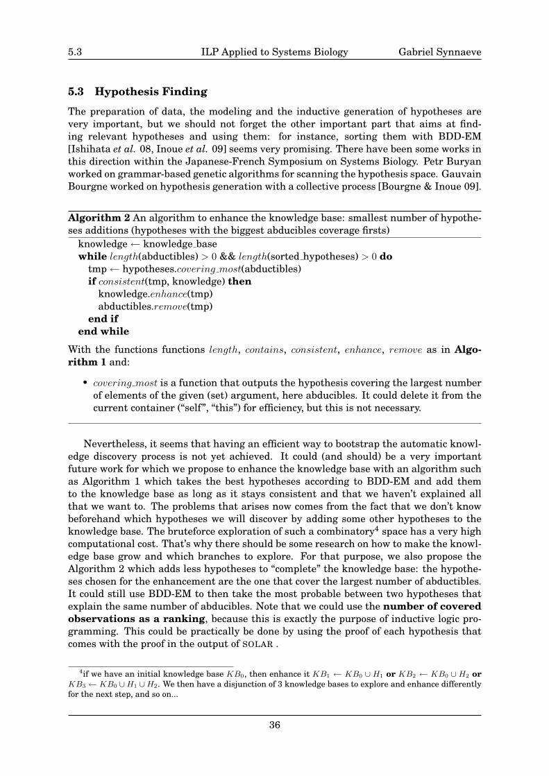
5.3 ILP Applied to Systems Biology Gabriel Synnaeve
5.3 Hypothesis Finding
The preparation of data, the modeling and the inductive generation of hypotheses arevery important, but we should not forget the other important part that aims at find-ing relevant hypotheses and using them: for instance, sorting them with BDD-EM[Ishihata et al. 08, Inoue et al. 09] seems very promising. There have been some works inthis direction within the Japanese-French Symposium on Systems Biology. Petr Buryanworked on grammar-based genetic algorithms for scanning the hypothesis space. GauvainBourgne worked on hypothesis generation with a collective process [Bourgne & Inoue 09].
Algorithm 2 An algorithm to enhance the knowledge base: smallest number of hypothe-ses additions (hypotheses with the biggest abducibles coverage firsts)
knowledge← knowledge basewhile length(abductibles) > 0 && length(sorted hypotheses) > 0 do
tmp← hypotheses.covering most(abductibles)if consistent(tmp, knowledge) then
knowledge.enhance(tmp)abductibles.remove(tmp)
end ifend while
With the functions functions length, contains, consistent, enhance, remove as in Algo-rithm 1 and:
• covering most is a function that outputs the hypothesis covering the largest numberof elements of the given (set) argument, here abducibles. It could delete it from thecurrent container (“self”, “this”) for efficiency, but this is not necessary.
Nevertheless, it seems that having an efficient way to bootstrap the automatic knowl-edge discovery process is not yet achieved. It could (and should) be a very importantfuture work for which we propose to enhance the knowledge base with an algorithm suchas Algorithm 1 which takes the best hypotheses according to BDD-EM and add themto the knowledge base as long as it stays consistent and that we haven’t explained allthat we want to. The problems that arises now comes from the fact that we don’t knowbeforehand which hypotheses we will discover by adding some other hypotheses to theknowledge base. The bruteforce exploration of such a combinatory4 space has a very highcomputational cost. That’s why there should be some research on how to make the knowl-edge base grow and which branches to explore. For that purpose, we also propose theAlgorithm 2 which adds less hypotheses to “complete” the knowledge base: the hypothe-ses chosen for the enhancement are the one that cover the largest number of abductibles.It could still use BDD-EM to then take the most probable between two hypotheses thatexplain the same number of abducibles. Note that we could use the number of coveredobservations as a ranking, because this is exactly the purpose of inductive logic pro-gramming. This could be practically be done by using the proof of each hypothesis thatcomes with the proof in the output of SOLAR .
4if we have an initial knowledge base KB0, then enhance it KB1 ← KB0 ∪ H1 or KB2 ← KB0 ∪ H2 orKB3 ← KB0 ∪H1 ∪H2. We then have a disjunction of 3 knowledge bases to explore and enhance differentlyfor the next step, and so on...
36
6.0 ILP Applied to Systems Biology Gabriel Synnaeve
6 Conclusion
We showed one way to discretize biology experiments into relevant levels to be usedwith ILP and logic programs in the large. An enhancement is already being investigatedfor the discretization. Moreover, based on this discretization of concentration into levels,we explained our processus to transform Michaelis-Menten analytical kinetics equationinto logic rules, we are not aware of any previous work in this direction. We think thatthis approach improves the accuracy of the metabolic flux analysis. Allowing for otherkinds of kinetic modeling (two substrate and/or two products reactions) would enable usto work with more complete models. As in [King et al. 05], this approach tries to enablethe behaviour of many ordinary differential equations while considering a symbolic model.
The more global approach of discretizing experimental data and using it inconjunction with automatically generated symbolic pathways extracted from KEGG[Kanehisa & Goto 00, Kanehisa et al. 08] can be applied regardless of the model cho-sen for infering new knowledge (see Fig.11 page 22). This approach can be genericallyapplied to turn quantitative results from systems biology into qualitative (symbolic) onesand should be seen as a step towards automation of hypothesis finding [King et al. 04].The process of evaluating hypotheses thanks to BDD-EM [Inoue et al. 09] is seen as agood method to find relevant knowledge among the large quantity of processed data. Par-ticularly here, we only need to rank (as opposed to evaluate) the hypotheses in regard toeach others (“pairwise”). The practical validity of this full process has been shown by theresults presented above while working in a well-known theoretical framework of induc-tive logic programming [Inoue 04, Mooney 97].
Still, our modeling can be improved. New highly probable knowledge could be ap-pended to the knowledge base to try and discover new hypotheses, being it through ab-duction (to find missing observations) or full clausal theory induction (to find rules thatgovern the system). This idea of revising the knowledge base is already presentin Ray et al. [Ray et al. 09] with a nonmonotonic approach. The pathway’s symbolicmodel, time and concentration discretization could be finer. For instance, experimentsdealing with more than 3 levels through a compute predicate implemented in SOLAR[Nabeshima et al. 03] and many time steps should be brought to a close on the Glycoly-sis and Pentose Phosphate pathways of another bacteria (representative of the eukaryotecells, this time), Saccharomyces Cerevisiae (yeast), with both real world data from ex-periments and simulated data. This will lead to use and test “iterative” (incremental)hypothesis finding process as this model is more complex and there are more discrete lev-els (9) and more discrete time steps.
This work can be seen as a proof of concept in the direction of mixing the realworld experimental values, analytical methods and logic-based approaches. The currentcontribution can be found in Fig.11 page 22. We intend to modify (fork) the currenthypothesis finding system found in Fig.4 page 13 towards something like Fig.20 page 38.
37
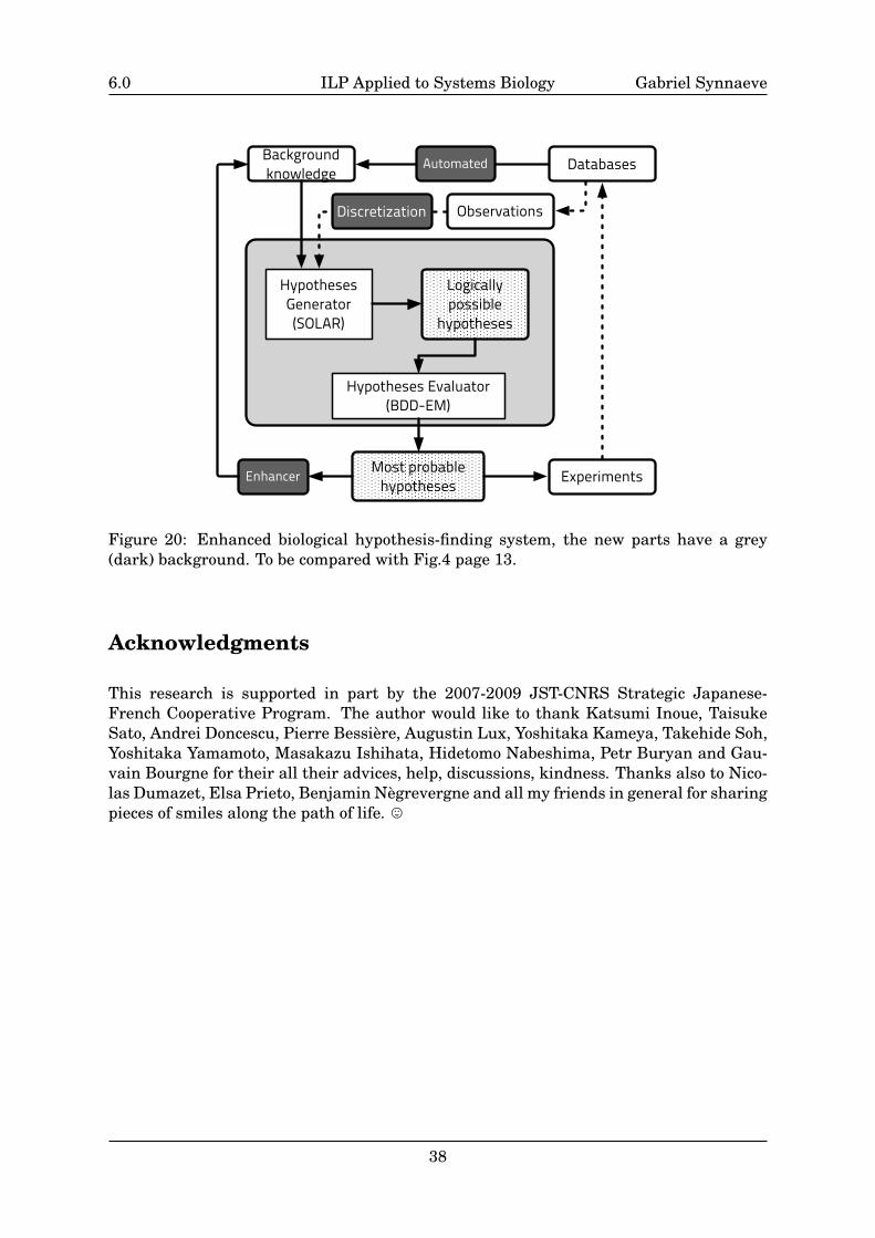
6.0 ILP Applied to Systems Biology Gabriel Synnaeve
Experiments
Logically possible
hypotheses
Databases
Hypotheses Generator(SOLAR)
Hypotheses Evaluator (BDD-EM)
Background knowledge
Observations
Most probable hypotheses
Discretization
Automated
Enhancer
Figure 20: Enhanced biological hypothesis-finding system, the new parts have a grey(dark) background. To be compared with Fig.4 page 13.
Acknowledgments
This research is supported in part by the 2007-2009 JST-CNRS Strategic Japanese-French Cooperative Program. The author would like to thank Katsumi Inoue, TaisukeSato, Andrei Doncescu, Pierre Bessiere, Augustin Lux, Yoshitaka Kameya, Takehide Soh,Yoshitaka Yamamoto, Masakazu Ishihata, Hidetomo Nabeshima, Petr Buryan and Gau-vain Bourgne for their all their advices, help, discussions, kindness. Thanks also to Nico-las Dumazet, Elsa Prieto, Benjamin Negrevergne and all my friends in general for sharingpieces of smiles along the path of life. ,
38
6.0 ILP Applied to Systems Biology Gabriel Synnaeve
References[Beal 03] Beal M. J.: Variational Algorithms for Approximate Bayesian Inference. PhD. Thesis,
Gatsby Computational Neuroscience Unit, University College London (2003).
[Benhamou 94] Benhamou F.: Interval Constraint Logic Programming. Lecture Notes In Com-puter Science; Vol. 910 (1994).
[Bourgne & Inoue 09] Bourgne G., Inoue K.: Towards a model of collective knowledge discovery.In Pre-Proceedings of the Workshop on Abductive and Inductive Knowledge Developpement(July 2009).
[Brants 00] Brants T.: TnT - A Statistical Part-of-Speech Tagger. In Proceedings of the Sixth Ap-plied Natural Language Processing Conference (2000).
[Chabrier-Rivier et al. 04] Chabrier-Rivier N., Fages F., Soliman S.: The biochemical abstract ma-chine BIOCHAM. CMSB, Springer (2004).
[Chen et al. 07] Chen J., Muggleton S., Santos J.: Abductive stochastic logic programs formetabolic network inhibition learning. MLG (2007).
[Chassagnole et al. 06] Chassagnole C., Rodrigues J. C., Doncescu A. and Tianruo Yang L.: Dif-ferential evolutionary algorithms for in vivo dynamic analysis of glycolysis and pentose phos-phate pathway in Escherichia Coli. In: A. Zomaya (ed.), Parallel Computing in Bioinformaticsand Computational Biology (2006).
[Cheeseman & Stutz 95] Cheeseman P. and Stutz J.: Bayesian classification (AutoClass): Theoryand results. Advances in Knowledge Discovery and Data Mining, pp.153-180, The MIT Press(1995).
[De Raedt 08] De Raedt L.: Logical and Relational Learning. Springer-Verlag (2008).
[Doncescu et al. 07] Doncescu, A., Inoue K., Yamamoto Y.: Knowledge Based Discovery in SystemsBiology Using CF-Induction. LNCS No 4570, pages 395-404 (2007).
[Flach & Kakas 00] Flach P. A., Kakas A. C.: Abduction and induction: Essays on their relationand integration. Kluwer (2000).
[Franco & Canela 84] Franco R. and Canela E.: Computer simulation of purine metabolism. Eu-ropean Journal of Biochemistry, 144:305-315 (1984).
[Gauvain & Lee 94] Gauvain J.-L. and Lee C.-H.: Maximum a posteriori estimation for multivari-ate Gaussian mixture observations of Markov chains. IEEE Transactions on Speech and AudioProcessing, Vol.2, Issue 2, pp.291-298 (1994).
[Geurts 01] Geurts P.: Pattern extraction for time-series classification. Proceedings of PKDD2001, 5th European Conference on Principles of Data Mining and Knowledge Discovery, LNAI2168, 115-127 (2001).
[Hofestadt & Thelen 98] Hofestadt R., Thelen S.: Quantitative Modeling of Biochemical Net-works. In In Silico Biology (Journal), ISSN: 1386-6338, Vol.1, N 1/1998, p.39-53 (1998).
[Inoue 92] Inoue, K.: Linear resolution for consequence finding. Artificial Intelligence 56:301-353(1992).
[Inoue 04] Inoue K.: Induction as consequence finding. Machine Learning, 55:109–135 (2004).
[Inoue et al. 09] Inoue K., Sato T., Ishihata M., Kameya Y. and Nabeshima H.: Evaluating ab-ductive hypotheses using and EM algorithm on BDDs. IJCAI-09, to appear, in Proceedings ofIJCAI-09 (2009).
39
6.0 ILP Applied to Systems Biology Gabriel Synnaeve
[Ishihata et al. 08] Ishihata M., Kameya Y., Sato T., Minato S.: Propositionalizing the EM algo-rithm by BDDs. Technical Report TR08-0004, Dept. of Computer Science, Tokyo Institute ofTechnology (2008)
[Ji et al. 06] Ji S., Krishnapuram B., and Carin L.: Variational Bayes for continuous hiddenMarkov models and its application to active learning. IEEE Transactions on Pattern Anal-ysis and Machine Intelligence, Vol.28, Issue 4, pp.522-532 (2006).
[Kanehisa & Goto 00] Kanehisa M. and Goto S.; KEGG: Kyoto Encyclopedia of Genes andGenomes. Nucleic Acids Res. 28, 27-30 (2000).
[Kanehisa et al. 08] Kanehisa M., Araki M., Goto S., Hattori M., Hirakawa M., Itoh M., KatayamaT., Kawashima S., Okuda S., Tokimatsu T., and Yamanishi Y.; KEGG for linking genomes tolife and the environment. Nucleic Acids Res. 36, D480-D484 (2008).
[Keogh et al. 05] Keogh E., Lin J. and Fu A.: HOT SAX: efficiently finding the most unusual timeseries subsequence. 5th IEEE International Conference on Data Mining (2005).
[Kersting & De Raedt 01] Kersting K., De Raedt L.: Adaptive Bayesian Logic Programs. In: Rou-veirol C., Sebag M. (eds.) ILP 2001. LNCS (LNAI), vol. 2157, Springer, Heidelberg (2001).
[King et al. 05] King R., Garrett S., Coghill G.: On the use of qualitative reasoning to simulateand identify metabolic pathways. Bioinformatics 21(9):2017-2026 (2005).
[King et al. 04] King R.D., Whelan K.E., Jones F.M., Reiser P.G.K., Bryant C.H., Muggleton S.H.,Kell D.B. & Oliver S.G.: Functional genomic hypothesis generation and experimentation by arobot scientist. Nature 427, 247-252 (2004).
[Kitano 02] Kitano H.: Systems Biology Toward System-level Understanding of Biological Sys-tems Kitano. In Science Vol. 295. no. 5560, pp. 1662-1664 (2002).
[Lee 67] Lee C.T.: A completeness theorem and computer program for finding theorems deriv-able from given axioms. Ph.D. thesis, Dept. of Electrical Engineering and Computer Science,University of California, Berkeley (1967).
[Lin et al. 07] Lin J., Keogh E., Wei L. and Lonardi S.: Experiencing SAX: a novel symbolic rep-resentation of time series. Data Mining and Knowledge Discovery, Vol.15, No.2, pp.107-144(2007).
[Mauch et al. 00] Mauch K., Vaseghi S., Reuss M.: Quantitative Analysis of Metabolic and Signal-ing Pathways in Saaharomyces cerevisiae. Bioreaction Engineering: Modeling and Control,Springer Verlag (2000).
[Mirrahmi et al. 05] Mirrahimi E., Rouchon P., Turinici G.: Lyapunov control of bilinearSchrodinger equations. Automatica 41(11):1987-1994 (2005).
[Mooney 97] R. J. Mooney: Integrating abduction and induction in machine learning. In WorkingNotes of the IJCAI97 Workshop on Abduction and Induction in AI, 37–42 (1997).
[Morchen et al. 05] Morchen F., Ultsch A.: Optimizing time Series Discretization for KnowledgeDiscovery. Proc. of KDD-05, pp.660-665 (2005).
[Muggleton 95] Muggleton S.: Inverse Entailment and Progol. New Generation Computing, Spe-cial issue on Inductive Logic Programming, 13:3-4 pp245-286 (1995).
[Muggleton & Chen 08] Muggleton S., Chen J.: A Behavioral Comparison of Some ProbabilisticLogic Models. Lecture Notes in Computer Science, Springer (2008).
[Nabeshima et al. 03] Nabeshima H., Iwanuma K., and Inoue K.: SOLAR : A ConsequenceFinding System for Advanced Reasoning. Proceedings of the 11th International ConferenceTABLEAUX 2003, LNAI, Vol. 2796, pp. 257-263, Springer (2003).
40
6.0 ILP Applied to Systems Biology Gabriel Synnaeve
[Nabeshima et al. 08] Nabeshima H., Iwanuma K., and Inoue K.: Completeness of pruning meth-ods for consequence finding procedure SOL. Proceedings of the LPAR 2008 Workshops, Knowl-edge Exchange: Automated Provers and Proof Assistants, and the 7th International Workshopon the Implementation of Logics (2008).
[Nienhuys-Cheng & De Wolf 97] Nienhuys-Cheng S.H., De Wolf R.: Foundations of inductive logicprogramming. LNAI 1228, Springer (1997).
[Peters-Wendisch et al. 01] Peters-Wendisch P. G., Schiel B., Wendisch V. F., Efstratios KatsoulidisE., Mockel B.: Pyruvate Carboxylase is a Major Bottleneck for Glutamate and Lysine Produc-tion by Corynebacterium glutamicum. J. Mol. Microbiol. Biotechnol. 3(2) (2001).
[Rabiner 89] Rabiner L.R.: A tutorial on hidden Markov models and selected applications inspeech recognition. Proc. of the IEEE Vol.77, No.2 (1989).
[Ray et al. 09] Ray O., Whelan K., King R.: A nonmonotonic logical approach for modelling and re-vising metabolic networks. Complex, Intelligent and Software Intensive Systems, IEEE Com-puter Society (2009).
[Reder 88] Reder C.: Metabolic control theory: a structural approach. Journal of theoretical Biol-ogy (1988).
[Sato 98] Sato T.: Modeling Scientific Theories as PRISM Programs. In Proceedings of ECAI98Workshop on Machine Discovery (1998).
[Savitzky & Golay 64] Savitzky A., Golay M.J.E.: Smoothing and Differentiation of Data by Sim-plified Least Squares Procedures. Analytical Chemistry 36 (8): 1627–1639 (1964).
[Schwarz 78] Schwarz G.: Estimating the dimension of a model. Annals of Statistics, Vol.6, No.2,pp.461-464 (1978).
[Tamaddoni-Nezhad et al. 06] Tamaddoni-Nezhad A., Chaleil R., Kakas A., and Muggleton S.H.:Application of abductive ILP to learning metabolic network inhibition from temporal data.Machine Learning, 64:209-230 (2006).
[Yamamoto 97] Yamamoto A.: Which hypotheses can be found with inverse entailment? Lecturenotes in computer science (LNCS) ISSUE 1297, pages 296-308, Springer (1997).
[Yamamoto et al. 08] Yamamoto Y., Inoue K., Doncescu A.: Estimation of Possible Reaction Statesin Metabolic Pathways using Inductive Logic Programming. In Proc. of 22nd InternationalConference on Advanced Information Networking and Applications (2008).
[Waser et al. 83] Waser M., Garfinkel L., Kohn C., and GarfinkelD .: Computer Modeling of MusclePhosphofructokinase. Journal of Theoretical Biology, 103:295-312 (1983).
41
6.0 ILP Applied to Systems Biology Gabriel Synnaeve
Glossary
abduction find hypotheses that are ground or existentially quantified formulaes (miss-ing facts or data). 3, 7
allosteric regulation regulation of an enzyme (or other protein) by binding an effectormodule at a protein’s site that is different from the active one. 10
anabolism synthesis of large molecules and structural components of the cell (proteins,RNA, DNA, lipids) from smaller substrates and chemical energy. 6
Baum-Welch algorithm generalized EM algorithm that computes maximum likelihoodestimates and posterior mode estimates for the parameters (transition and emissionprobabilities) of an HMM, when given only emissions as training data.. 25
catabolism degradation of an external substrate (ex: Sugar) into smaller chemical prod-ucts to provide energy (ex: stored in ATP). 6
clausal theory finite conjunctive set of clauses. 7
clause disjunction of litterals,∨ni=1Ai. 3, 7
expectation-maximization iterative algorithm to find the maximum likelihood esti-mates of parameters in a probabilistic model. 23, 30
hidden Markov model (⊂ Bayesian networks) statistical model in which the systemmodeled is assumed to be a Markov process with unobserved states. 17, 21
Horn clause definite or negative clause, ex: {¬A ∨ ¬B ∨ C} ⇔ {A ∧B ⇒ C}. 7
induction find hypotheses that are unversally quantified formulaes (missing rules). 3, 7
inhibition decreasing an enzyme activity (and so reaction rate) by binding somemolecule to it at a strategic location. 6
integrity constraint negative clause, ex: {¬A ∨ ¬B ∨ ¬C}. 7
likelihood function given a parametrized density function x 7→ f(x|θ), the likehoodfunction is θ 7→ f(x|θ) ,written L(θ;x) = f(x|θ). 23
metabolic pathway sequence of reactions occuring within the cell, which are intercon-nected via substrates, catalyzed by enzymes and often requiring other cofactors. 3,4, 6
metabolism set of reactions that maintain life. 3
metabolite intermediate and/or final chemical product of a metabolism. 3, 5
subsumption (subsomption) Cθ-subsumes D iff ∃θ such that, syntactically, Cθ ⊆ D. Wealso say that C is more general than D.. 7
42
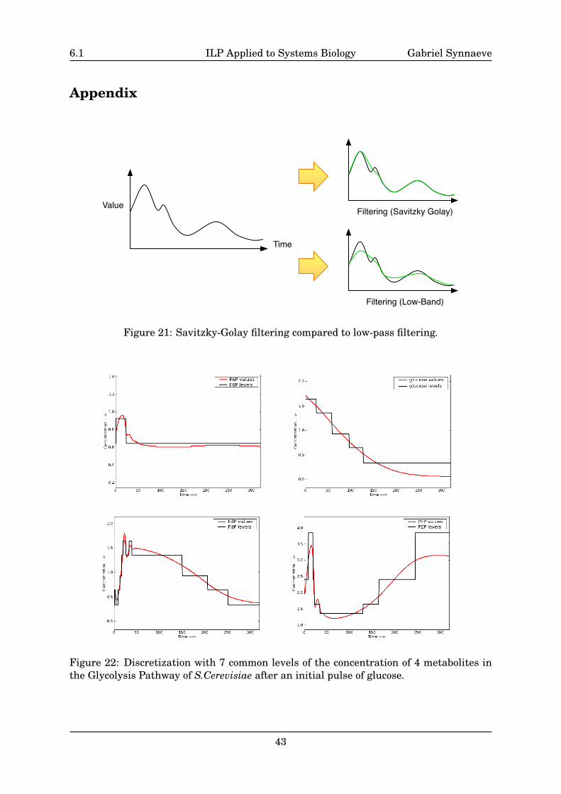
6.1 ILP Applied to Systems Biology Gabriel Synnaeve
Appendix
Filtering (Savitzky Golay)
Filtering (Low-Band)
Value
Time
Figure 21: Savitzky-Golay filtering compared to low-pass filtering.
Figure 22: Discretization with 7 common levels of the concentration of 4 metabolites inthe Glycolysis Pathway of S.Cerevisiae after an initial pulse of glucose.
43
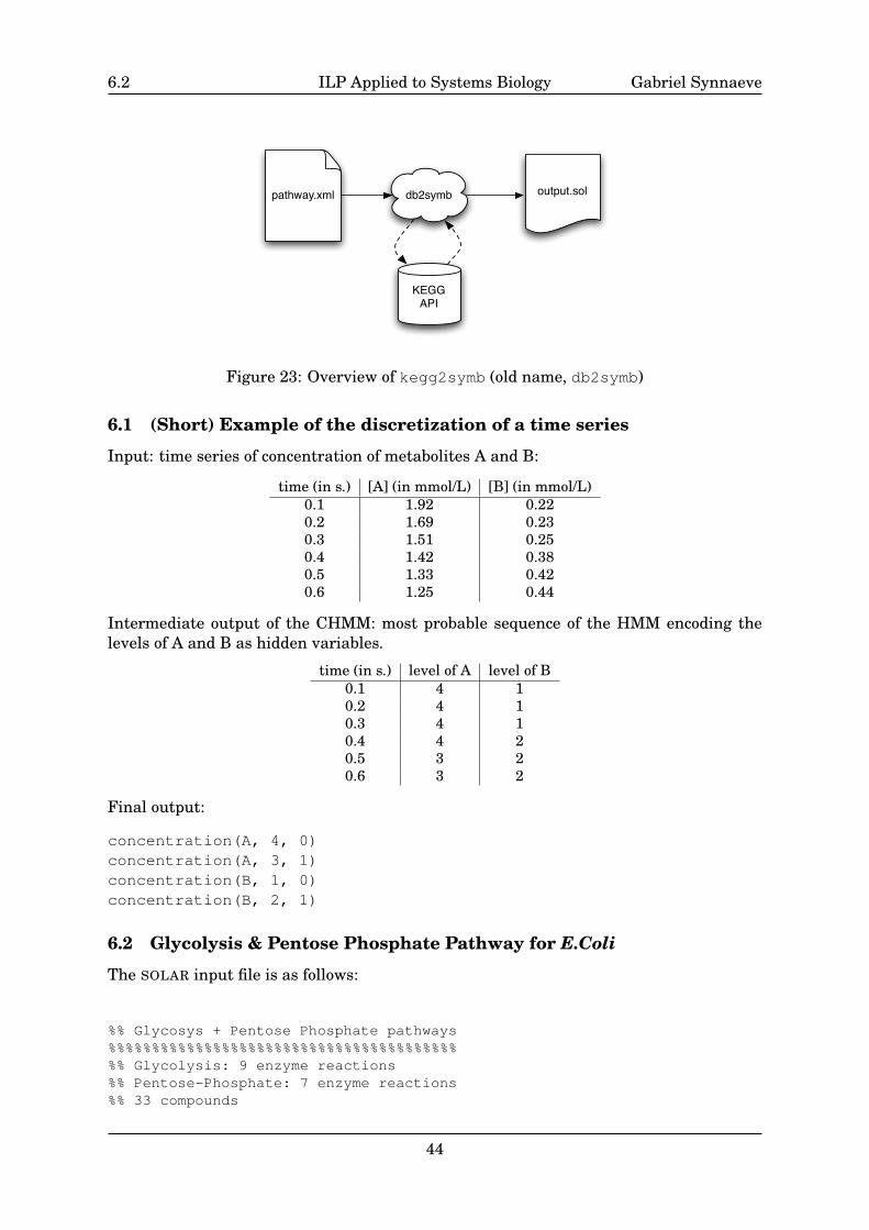
6.2 ILP Applied to Systems Biology Gabriel Synnaeve
pathway.xml db2symb
KEGG API
output.sol
Figure 23: Overview of kegg2symb (old name, db2symb)
6.1 (Short) Example of the discretization of a time series
Input: time series of concentration of metabolites A and B:
time (in s.) [A] (in mmol/L) [B] (in mmol/L)0.1 1.92 0.220.2 1.69 0.230.3 1.51 0.250.4 1.42 0.380.5 1.33 0.420.6 1.25 0.44
Intermediate output of the CHMM: most probable sequence of the HMM encoding thelevels of A and B as hidden variables.
time (in s.) level of A level of B0.1 4 10.2 4 10.3 4 10.4 4 20.5 3 20.6 3 2
Final output:
concentration(A, 4, 0)concentration(A, 3, 1)concentration(B, 1, 0)concentration(B, 2, 1)
6.2 Glycolysis & Pentose Phosphate Pathway for E.Coli
The SOLAR input file is as follows:
%% Glycosys + Pentose Phosphate pathways%%%%%%%%%%%%%%%%%%%%%%%%%%%%%%%%%%%%%%%%%% Glycolysis: 9 enzyme reactions%% Pentose-Phosphate: 7 enzyme reactions%% 33 compounds
44

6.2 ILP Applied to Systems Biology Gabriel Synnaeve
%% 18 enzymes%%%%%%%%%%%%%%%%%%%%%%%%%%%%%%%%%
%%%%%%%%%%%%%%%%%%%%% Reactions%%%%%%%%%%%%%%%%%
%%Predicates:%reaction_1(Substrate, Enzyme1, Product).%reaction_2(Substrate1,Enzyme1, Product,Enzyme2).%reaction_3(Substrate1, Substrate2, Substrate3, Enzyme, Product).
% Phosphotransferase systemcnf(r1_1, axiom, [reaction_2(glucose,atp,g6p,adp)]).
%Embden-Meyerhof-Parnas pathwaycnf(r2_1, axiom, [reaction_2(g6p,atp,f6p,adp)]).cnf(r2_2, axiom, [reaction_2(f6p,atp,fdp,adp)]).cnf(r2_3, axiom, [reaction_2(fdp,atp,gap,dhap)]).cnf(r2_4, axiom, [reaction_2(dhap,atp,gap,adp)]).cnf(r2_5, axiom, [reaction_2(gap,nad,pg3,nadh)]).cnf(r2_6, axiom, [reaction_2(pg3,atp,pep,adp)]).cnf(r2_7, axiom, [reaction_2(pep,adp,pyr,atp)]).cnf(r2_8, axiom, [reaction_2(pyr,nad,accoa,nadh)]).
%Pentose phosphate pathwaycnf(r3_1, axiom, [reaction_2(g6p,nadp,pg6,nadph)]).cnf(r3_2, axiom, [reaction_2(pg6,nadp,ribu5p,nadph)]).cnf(r3_3, axiom, [reaction_2(ribu5p,atp,rib5p,adp)]).cnf(r3_4, axiom, [reaction_2(ribu5p,atp,xyl5p, adp)]).cnf(r3_5, axiom, [reaction_2(rib5p,xyl5p,sed7p,gap)]).cnf(r3_6, axiom, [reaction_2(sed7p,gap,f6p,e4p)]).cnf(r3_7, axiom, [reaction_2(xyl5p,e4p,f6p,gap)]).
%%%%%%%%%%%%%%%%%%%%%%%% Causal relations%%%%%%%%%%%%%%%%%%%%%%
%%% On the predicate ‘‘reaction_2’’
cnf(un, axiom, [-reaction_2(Substrate1,Enzyme1, Product, Enzyme2),-concentration(Substrate1, 0, 0),-concentration(Enzyme2, 2, 0),-concentration(Product, L, 0),concentration(Product, L, 1)%%% concentration(Product, 0, 1)
]).
cnf(un, axiom, [-reaction_2(Substrate1, Enzyme1, Product, Enzyme2),-concentration(Substrate1, 1, 0),-concentration(Enzyme2, 1, 0),concentration(Product, 1, 1)
]).
45
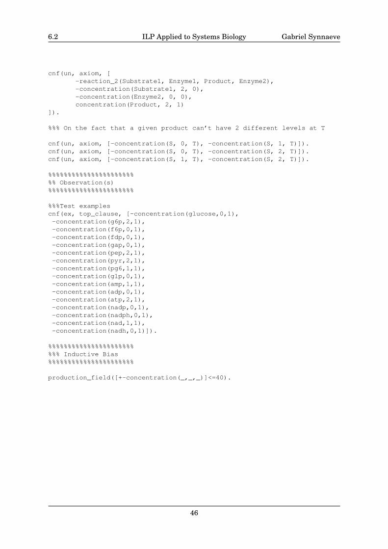
6.2 ILP Applied to Systems Biology Gabriel Synnaeve
cnf(un, axiom, [-reaction_2(Substrate1, Enzyme1, Product, Enzyme2),-concentration(Substrate1, 2, 0),-concentration(Enzyme2, 0, 0),concentration(Product, 2, 1)
]).
%%% On the fact that a given product can’t have 2 different levels at T
cnf(un, axiom, [-concentration(S, 0, T), -concentration(S, 1, T)]).cnf(un, axiom, [-concentration(S, 0, T), -concentration(S, 2, T)]).cnf(un, axiom, [-concentration(S, 1, T), -concentration(S, 2, T)]).
%%%%%%%%%%%%%%%%%%%%%%%% Observation(s)%%%%%%%%%%%%%%%%%%%%%%
%%%Test examplescnf(ex, top_clause, [-concentration(glucose,0,1),-concentration(g6p,2,1),-concentration(f6p,0,1),-concentration(fdp,0,1),-concentration(gap,0,1),-concentration(pep,2,1),-concentration(pyr,2,1),-concentration(pg6,1,1),-concentration(g1p,0,1),-concentration(amp,1,1),-concentration(adp,0,1),-concentration(atp,2,1),-concentration(nadp,0,1),-concentration(nadph,0,1),-concentration(nad,1,1),-concentration(nadh,0,1)]).
%%%%%%%%%%%%%%%%%%%%%%%%% Inductive Bias%%%%%%%%%%%%%%%%%%%%%%
production_field([+-concentration(_,_,_)]<=40).
46
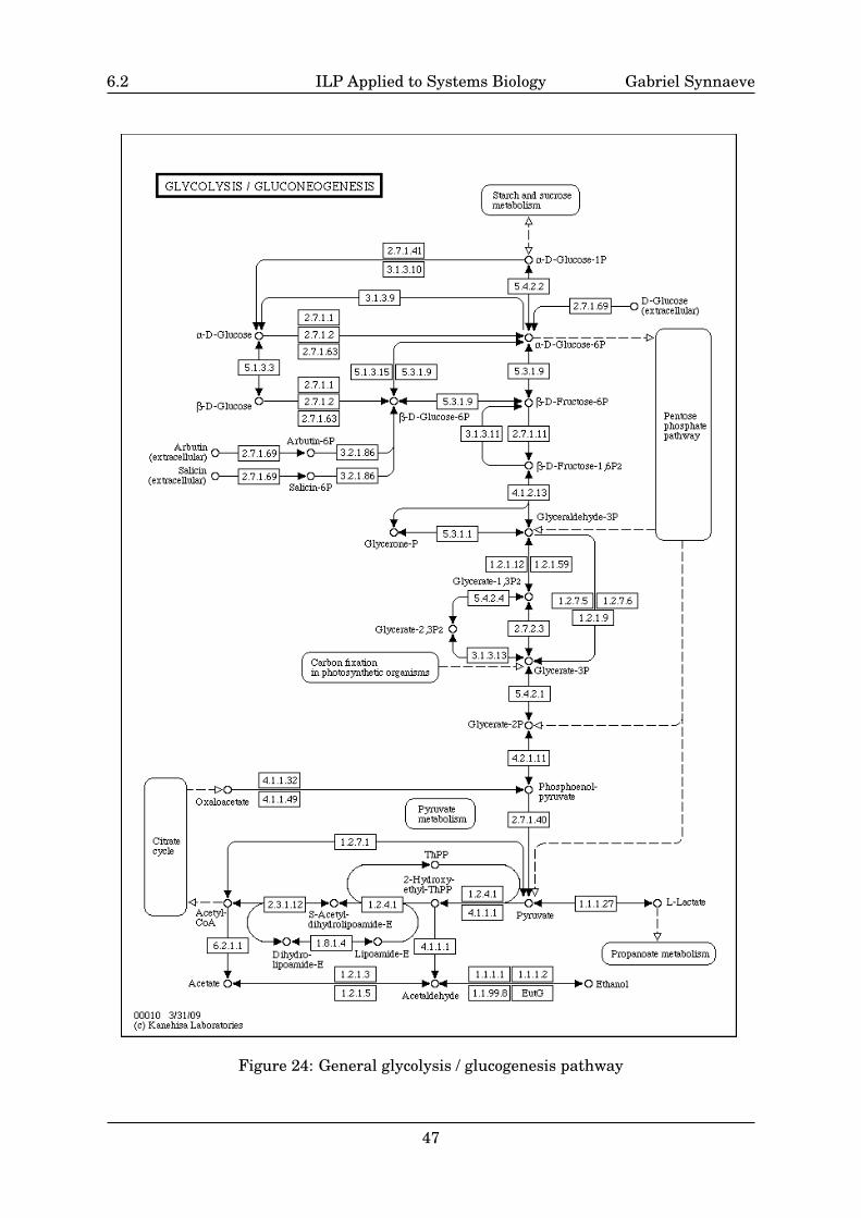
6.2 ILP Applied to Systems Biology Gabriel Synnaeve
Figure 24: General glycolysis / glucogenesis pathway
47
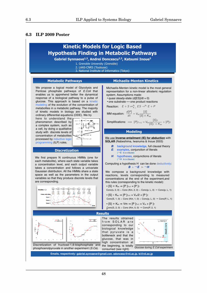
6.3 ILP Applied to Systems Biology Gabriel Synnaeve
6.3 ILP 2009 Poster
Kinetic Models for Logic Based Hypothesis Finding in Metabolic Pathways
Emails, respectively: [email protected], [email protected], [email protected]
Gabriel Synnaeve1,3, Andrei Doncescu2,3, Katsumi Inoue3
We use Inverse entailment (IE) for abduction withSOLAR (Nabeshima, Iwanuma & Inoue 2003)
B: background knowledge, full clausal theoryE: examples, conjunction of literals
(¬E is a clause)H: hypotheses, conjunctions of literals
(¬H is a clause)
Computing a hypothesis H can be done deductively: B ∧ ¬E ⊨ ¬H
1. Grenoble University (Grenoble)2. LAAS-CNRS (Toulouse)3. National Institute of Informatics (Tokyo)
Metabolic Pathways Michaelis-Menten Kinetics
Discretization
We propose a logical model of Glycolysis and Pentose phosphate pathways of E.Coli that enables us to apprehend better the dynamical response of a biological pathway to a pulse of glucose. This approach is based on a kinetic modeling of the evolution of the concentration of metabolites in a metabolic pathway. The majority of kinetic models in biology are studied with ordinary differential equations (ODE). We try
• [S] ≃ Km ⇒ [P ]T+1 = Vm/2 + [P ]TConc(S, 1, 0) ∧ Conc (Km, 1, 0) ∧ Conc(p, L, 0) → Conc(P, L, 1)
• [S] ≫ Km ⇒ Vm ⇒ [P ]T+1 = Vm + [P ]T
•Conc(S, 2, 0) ∧ Conc (Km, 0, 0) → Conc(P, 2, 1)
Conc(s, 0, 0) ∧ Conc (Km, 2, 0) ∧ Conc(p, L, 0) → Conc(p, L, 1)• [S] ≪ Km ⇒ [P ]T+1 = [P ]T
here to understand the phenomenon described by a complex system, such as a cell, by doing a qualitative study with discrete levels of concentration of metabolites processed by inductive logic programming (ILP) rules.
E + S !k1k−1 ES →
k2 E + P
d [P ]
dt= Vm
[S]
[S] +Km
=⇒ [P ]T+1 = Vm[S]T
[S]T +Km+ [P ]T
Michaelis-Menten kinetic model is the most general representation for a non-linear allosteric regulation system. Assumptions made: • quasi steady-state (d[ES]/dt ≈ 0)• one substrate ↔ one product reactions
MM equation:
Reaction:
Simplifications:
We first prepare N continuous HMMs (one for each metabolite), where each state variable takes a concentration level, and each output variable takes a concentration and follows a univariate Gaussian distribution. All the HMMs share a state space as well as the parameters in the output variables so that they produce discrete levels that are corresponding.
We compose a background knowledge with reactions, levels corresponding to measured concentrations at the end of the experiment,and this rules (corresponding to the kinetic model):
Modeling
ResultsThe results obtained f r o m S O L A R a r e corresponding to our biological knowledge t h a t p y r u v a t e i s a bottleneck and that the glucose, that was in high concentration at the beginning, is totally consumed (see right).
Discretization of fructose-1,6-bisphosphate and phosphoenolpyruvate in another experiment (S.Ce). Glucose during E.Coli experiment
48