INDUCED BIAS IN ATTENUATION MEASUREMENTS TAKENFROM COMMERCIAL MICROWAVE LINKS

Jonatan Ostrometzky∗, Adam Eshel†, Pinhas Alpert†, and Hagit Messer∗ Fellow, IEEE∗School of Electrical Engineering, Tel Aviv University

†Department of Geosciences, Tel Aviv University

Abstract—Cellular backhaul networks usually consist of com-mercial microwave links, known to be sensitive to weatherconditions. The management network systems usually providerecords of measurements of the transmitted and the receivedsignals levels from the different microwave links for monitoringand analyzing the network performance. Many of them logonly the minimum and the maximum levels of the transmittedand the received signals in pre-set intervals (usually 15-minute).Moreover, only quantized version of these measurements arelogged. In the last decade it has been proposed to use theseexisting measurements for rainfall monitoring. In this paper weanalyze the effects of the quantizer and the min/max operatorson commercial microwave links signals levels measurements. Weshow that the quantization process, in combination with themin/max operators, adds bias to the measurements which canbe significant. We then propose a method to calculate this bias,and demonstrate our findings using measurements from actualcommercial microwave links.

Index Terms—Quantization Noise, Microwave Networks, Pre-cipitation Attenuation

I. INTRODUCTION

Current cellular communication networks are based, at leastpartly, on Commercial Microwave Links (CMLs). In order toinspect and analyse the performance of these networks, currentNetwork Management Systems (NMS) constantly monitor theCMLs Transmitted Signal Level (TSL) and Received SignalLevel (RSL).

The NMS help in monitoring the Link Budget (LB), as it iscritical that the LB will not breach the Fading Margin limits ofthe CML. Thus, many NMS will log only the minimum andthe maximum values of the observed RSL and TSL values,usually in 15-minute intervals, using a rough quantizer [5],[16], as these relatively low-resolution datasets are sufficientfor the LB monitoring purposes [9].

Furthermore, since CMLs signals are known to be sensitiveto rain [11], it was suggested back in 2006 to use the TSL andRSL available datasets for rain monitoring [17]. Since then, avast number of studies suggested different methods and tech-niques which use the TSL and RSL available measurementsfor rain monitoring [7], [14], [19], rainfall maps plotting [15],[22], classification and estimation of snow and sleet [1], [18],fog monitoring [4], the detection of dew [10], and recently,the detection of air-pollution [3].

On the other hand, although sufficient for network moni-toring, quantized min/max TSL and RSL values given at 15-minute intervals have proven to be sub-optimal for environ-mental monitoring purposes. Thus, it was suggested to dealwith the non-linear min/max operators either by performing

calibration of different model parameters [20], by implement-ing weighted average of the minimum and the maximum val-ues [21], or by bypassing this limitation by directly accessingthe CML hardware, and retrieve the instantaneous RSL/TSLmeasurements themselves [2]. It is worth noting, that unlikethe min/max operators, the quantizer is usually a property ofthe hardware itself, and thus, even accessing the CML directlyand retrieving the instantaneous measurements sill results inquantized data [2].

The fact that the available RSL and TSL measurements passa quantizer was generally ignored. Indeed, Goldstein et. al. [6]discussed the normalization of the quantization error in regardto the CMLs length, and suggested to include the normalizedquantization error within the covariance matrix of the noise.And, although it was shown that the quantization processmight introduce errors [13], these errors were considered tobe unavoidable and relatively small for the purpose of rainmonitoring using CMLs attenuation measurements [16], [23],and thus, did not attract special interest.

In this paper we show that the combination of a quantizerwith a non-linear min/max operator induces a non-negligiblebias to the output value. We show that this bias, unlesscompensated, may introduce a bias to the LB calculations,and may cause an over-estimation of the rain. Furthermore,we show that the expected value of this bias can be calcu-lated using the available minimum and maximum RSL andTSL measurements during dry periods. We demonstrate ourfindings using actual measurements taken from CMLs.

The rest of the paper is organized as follows: SectionII presents the theory and establishes the bias calculationmethodology. Section III describes the experimental demon-stration, and discusses the results. Lastly, Section IV concludesthis paper.

II. THEORY AND METHODOLOGY

The nearest-neighbour (or a ”round”) quantizer q(x) isdefined by:

y = q(x) = L · round( x

L

)(1)

where x is the input signal, y is the (quantized) output, and0 < L ∈ R is the quantization interval. Note, that q(x) is saidto be both uniform and symmetric quantizer [8].

A. Combination of the Quantizer q(x) and the Min/Max Op-erators

First, note that the specific order of the operations in regardto the min or max operators, and the quantizer q(x), does

3744978-1-5090-4117-6/17/$31.00 ©2017 IEEE ICASSP 2017

not change the outcome, as described in Lemma 1:

Lemma 1. For any given {xi ∈ R} : i ∈ [1, 2, · · · , n],

max (q(x1), q(x2), · · · , q(xn)) = q (max(x1, x2, · · · , xn))(2)

Proof.

max (q(x1), · · · , q(xn)) =

= L ·max(round

(x1

L

), · · · , round

(xn

L

))=

= L · round((max(x1, · · · , xn))

L

)=

= q (max (x1, · · · , xn)) (3)

Similarly, Lemma 1 applies in regard to the min operator.In order to inspect the combined effect of applying a min or

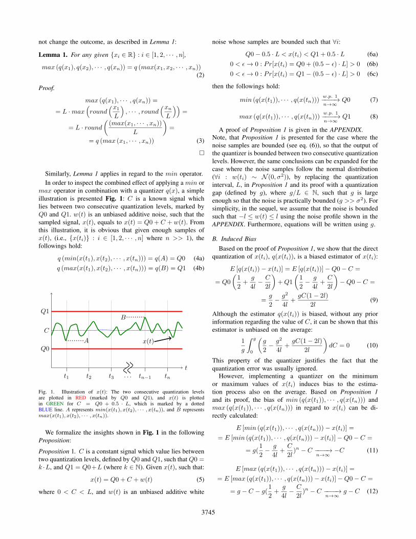
max operator in combination with a quantizer q(x), a simpleillustration is presented Fig. 1: C is a known signal whichlies between two consecutive quantization levels, marked byQ0 and Q1. w(t) is an unbiased additive noise, such that thesampled signal, x(t), equals to x(t) = Q0 + C + w(t). Fromthis illustration, it is obvious that given enough samples ofx(t), (i.e., {x(ti)} : i ∈ [1, 2, · · · , n] where n >> 1), thefollowings hold:

q (min(x(t1), x(t2), · · · , x(tn))) = q(A) = Q0 (4a)q (max(x(t1), x(t2), · · · , x(tn))) = q(B) = Q1 (4b)

t

x(t)Q0

Q1

C

B

A

t1 t2 t3 tn−1 tn· · ·

Fig. 1. Illustration of x(t): The two consecutive quantization levelsare plotted in RED (marked by Q0 and Q1), and x(t) is plottedin GREEN for C = Q0 + 0.5 · L, which is marked by a dottedBLUE line. A represents min(x(t1), x(t2), · · · , x(tn)), and B representsmax(x(t1), x(t2), · · · , x(tn)).

We formalize the insights shown in Fig. 1 in the followingProposition:

Proposition 1. C is a constant signal which value lies betweentwo quantization levels, defined by Q0 and Q1, such that Q0 =k ·L, and Q1 = Q0+L (where k ∈ N). Given x(t), such that:

x(t) = Q0 + C + w(t) (5)

where 0 < C < L, and w(t) is an unbiased additive white

noise whose samples are bounded such that ∀i:

Q0− 0.5 · L < x(ti) < Q1 + 0.5 · L (6a)0 < ϵ → 0 : Pr[x(ti) = Q0 + (0.5− ϵ) · L] > 0 (6b)0 < ϵ → 0 : Pr[x(ti) = Q1− (0.5− ϵ) · L] > 0 (6c)

then the followings hold:

min (q(x(t1)), · · · , q(x(tn)))w.p. 1−−−−→n→∞

Q0 (7)

max (q(x(t1)), · · · , q(x(tn)))w.p. 1−−−−→n→∞

Q1 (8)

A proof of Proposition 1 is given in the APPENDIX.Note, that Proposition 1 is presented for the case where thenoise samples are bounded (see eq. (6)), so that the output ofthe quantizer is bounded between two consecutive quantizationlevels. However, the same conclusions can be expanded for thecase where the noise samples follow the normal distribution(∀i : w(ti) ∼ N (0, σ2)), by replacing the quantizationinterval, L, in Proposition 1 and its proof with a quantizationgap (defined by g), where g/L ∈ N, such that g is largeenough so that the noise is practically bounded (g >> σ2). Forsimplicity, in the sequel, we assume that the noise is boundedsuch that −l ≤ w(t) ≤ l using the noise profile shown in theAPPENDIX. Furthermore, equations will be written using g.

B. Induced BiasBased on the proof of Proposition 1, we show that the direct

quantization of x(ti), q(x(ti)), is a biased estimator of x(ti):

E [q(x(ti))− x(ti)] = E [q(x(ti))]−Q0− C =

= Q0

(1

2+

g

4l− C

2l

)+Q1

(1

2− g

4l+

C

2l

)−Q0− C =

=g

2− g2

4l+

gC(1− 2l)

2l(9)

Although the estimator q(x(ti)) is biased, without any priorinformation regarding the value of C, it can be shown that thisestimator is unbiased on the average:

1

g

∫ g

0

(g

2− g2

4l+

gC(1− 2l)

2l

)dC = 0 (10)

This property of the quantizer justifies the fact that thequantization error was usually ignored.

However, implementing a quantizer on the minimumor maximum values of x(ti) induces bias to the estima-tion process also on the average. Based on Proposition 1and its proof, the bias of min (q(x(t1)), · · · , q(x(tn))) andmax (q(x(t1)), · · · , q(x(tn))) in regard to x(ti) can be di-rectly calculated:

E [min (q(x(t1)), · · · , q(x(tn)))− x(ti)] =

= E [min (q(x(t1)), · · · , q(x(tn)))− x(ti)]−Q0− C =

= g(1

2− g

4l+

C

2l)n − C −−−−→

n→∞−C (11)

E [max (q(x(t1)), · · · , q(x(tn)))− x(ti)] =

= E [max (q(x(t1)), · · · , q(x(tn)))− x(ti)]−Q0− C =

= g − C − g(1

2+

g

4l− C

2l)n − C −−−−→

n→∞g − C (12)

3745

Unlike q(x(ti)), both min (q(x(t1)), · · · , q(x(tn))) andmax (q(x(t1)), · · · , q(x(tn))) are biased also on the average:

min(q(x(ti)) :1

g

∫ g

0

(−C) dC = −g

2n >> 1 (13)

max(q(x(ti)) :1

g

∫ g

0

(g − C) dC =g

2n >> 1 (14)

From equations (13) and (14) two important conclusions arise:First, a combination of a min/max operator and a quantizerintroduces bias to the original measurements of x(ti), whichmay not be negligible. Second, this bias depends on thequantization gap, g.

C. Maximum and Minimum TSL and RSL Measurements

NMS monitor the TSL and the RSL of the CMLs. Thespecific sampling and logging protocols varies between thehardware vendors. For instance, EricssonTM systems usuallysample the signal level at 10-seconds intervals, and save theminimum and the maximum values every 15 minutes, usinga standard quantization intervals of 1[dB] for the TSL, and0.3[dB] for the RSL [23].

During dry periods, the LB is considered to remain rel-atively constant [12], meaning that the transmitted power(defined by Tx) and the received power (defined by Rx)fluctuations are also limited. Thus, under the assumption thatthe minimum and the maximum TSL and RSL values areextracted from large enough instantaneous samples series (i.e.,n >> 1), Proposition 1 is valid, and can be used in orderto connect the CML path-loss (which equals to Tx − Rx)with the minimum channel attenuation (defined by Amin) andthe maximum channel attenuation (defined by Amax), whichyields:

Amin = TSLmin −RSLmax =

= (Tx− gT2)− (Rx+

gR2) =

= (Tx−Rx)− (gT2

+gR2) (15)

Amax = TSLmax −RSLmin =

= (Tx+gT2)− (Rx− gR

2) =

= (Tx−Rx) + (gT2

+gR2) (16)

where gT is the quantization gap of the TSL values, and gRis the quantization gap of the RSL values.

Next, subtracting eq. (15) from eq. (16), yields:

Adiff ≡ Amax −Amin = gT + gR (17)

which connects the extreme attenuation measurements withthe expected value of the bias.

And, although this calculation is made during dry periods,it can be assumed that the same expected value of the biasremains during rainy periods, as the rain does not affect thequantization intervals and levels. Thus, on average, the samebias occurs.

III. EXPERIMENTAL DEMONSTRATION

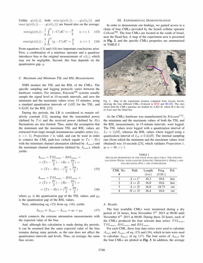
In order to demonstrate our findings, we gained access to achain of four CMLs provided by the Israeli cellular operatorCellcomTM. The four CMLs are located in the south of Israel,near the Dead-Sea. A map of the experiment area is presentedin Fig. 2, and the specific CMLs properties are summarizedin TABLE I.

Fig. 2. Map of the experiment location (captured from Google Earth),showing the four different CMLs (Colored in RED and BLUE). The siteswhich hold the CMLs antennas are marked by A,B,C,D, where B is the cityof Arad near the Dead-Sea.

As the CMLs hardware was manufactured by EricssonTM ,the minimum and the maximum values of both the TSL andthe RSL measurements, in 15-minute intervals, were logged.The TSL values were logged with a quantization interval ofLT ≡ 1[dB], whereas the RSL values where logged using aquantization interval of LR ≡ 0.3[dB]. The internal samplingrate (from which the minimum and the maximum values wereobtained) was 10-seconds [23], which validates Proposition 1,as n = 90 >> 1.

TABLE IDETAILED PROPERTIES OF THE FOUR AVAILABLE CMLS: THE SPECIFIC

LOCATION (PATH), PATH-LENGTH (LENGTH), FREQUENCY (FREQ.) ANDPOLARIZATION (POL.) ARE SUMMARIZED.

CML No. Path Length Freq. Pol.# (km) (GHz)

1 A ↔ C 10.3 18.6 hor2 A ↔ B 16.0 18.6 hor3 A ↔ B 16.0 18.73 ver4 B ↔ D 26.4 18.6 ver

A. Results

The four available CMLs were monitored during a dryperiod of 24 hours, from November 5th 2015 at 00:00 untilNovember 6th 2015 at 00:00. During these 24 hours, each ofthe CMLs produced the four relevant data series: TSLmin,TSLmax, RSLmin, and RSLmax.

For each CML, these four data series were used to calculateAmin and Amax, of eq. (15) and (16), which in turn were usedto calculate Adiff of eq. (17). The four series of Adiff forthe four CMLs are plotted in Fig. 3. In addition, the average

3746

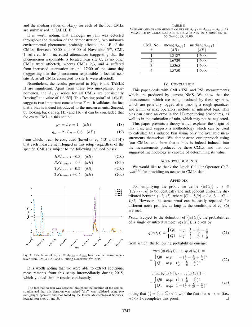
and the median values of Adiff for each of the four CMLsare summarized in TABLE II.

It is worth noting, that although no rain was detectedthroughout the duration of the demonstration1, two unknownenvironmental phenomena probably affected the LB of theCMLs: Between 00:00 and 03:00 of November 5th, CML1 suffered from increased attenuation (suggesting that thephenomenon responsible is located near site C, as no otherCMLs were affected), wheras CMLs 2,3, and 4 sufferedfrom increased attenuation around 17:00 of the same day(suggesting that the phenomenon responsible is located nearsite B, as all CMLs connected to site B were affected).

Nonetheless, the results presented in Fig. 3 and TABLEII are significant. Apart from these two unexplained phe-nomenon, the Adiff series for all CMLs are consistently”resting” at a value of 1.6[dB]. This ”resting point” of 1.6[dB]suggests two important conclusions: First, it validates the factthat a bias is indeed introduced to the measurements. Second,by looking back at eq. (15) and (16), it can be concluded thatfor every CML in this setup:

gT = LT = 1 (dB) (18)

gR = 2 · LR = 0.6 (dB) (19)

from which, it can be concluded (based on eq. (13) and (14))that each measurement logged in this setup (regardless of thespecific CML) is subject to the following induced biases:

RSLmin : −0.3 (dB) (20a)RSLmax : +0.3 (dB) (20b)TSLmin : −0.5 (dB) (20c)TSLmax : +0.5 (dB) (20d)

Fig. 3. Calculation of Adiff ≡ Amax −Amin based on the measurementstaken from CMLs 1,2,3 and 4, during November 5th 2015.

It is worth noting that we were able to extract additionalmeasurements from this setup intermediately during 2015,which yielded similar results consistently.

1The fact that no rain was detected throughout the duration of the demon-stration and that this duration was indeed ”dry”, was validated using tworain-gauges operated and monitored by the Israeli Meteorological Services,located near sites A and B.

TABLE IIAVERAGE (MEAN) AND MEDIAN VALUES OF Adiff ≡ Amax −Amin AS

MEASURED BY CMLS 1,2,3 AND 4, FROM 05-NOV-2015, 00:00 UNTIL06-NOV-2015, 00:00.

CML No. mean(Adiff ) median(Adiff )# (dB) (dB)

1 1.8187 1.60002 1.6729 1.60003 1.5365 1.60004 1.5750 1.6000

IV. CONCLUSION

This paper deals with CMLs TSL and RSL measurementswhich are produced by current NMS. We show that themeasurements which are being produced by these systems,which are generally logged after passing a rough quantizerand a min or max operators, include an inherited bias. Thisbias can cause an error in the LB monitoring procedures, aswell as in the estimation of rain, which may not be neglected.

This paper presents a theory which explains the origin ofthis bias, and suggests a methodology which can be usedto calculate this induced bias using only the available mea-surements themselves. We demonstrate our approach usingfour CMLs, and show that a bias is indeed induced intothe measurements produced by these CMLs, and that oursuggested methodology is capable of determining its value.

ACKNOWLEDGMENTS

We would like to thank the Israeli Cellular Operator Cell-comTM for providing us access to CMLs data.

APPENDIX

For simplifying the proof, we define {w(ti)} : i ∈[1, 2, · · · , n] to be identically and independent uniformly dis-tributed between (−l,+l), where |C − L/2| < l < L− |C −L/2|. However, the same proof can be easily repeated fordifferent noise profiles, as long as the conditions of eq. (6)are met.

Proof. Subject to the definition of {w(ti)}, the probabilitiesof a single quantized sample, q(x(ti)), is given by:

q(x(ti)) =

{Q0 w.p. 1

2 + L4l −

C2l

Q1 w.p. 12 − L

4l +C2l

(21)

from which, the following probabilities emerge:

min (q(x(t1)), · · · , q(x(tn))) =

=

{Q0 w.p. 1− ( 12 − L

4l +C2l )

n

Q1 w.p. ( 12 − L4l +

C2l )

n(22)

max (q(x(t1)), · · · , q(x(tn))) =

=

{Q0 w.p. ( 12 + L

4l −C2l )

n

Q1 w.p. 1− ( 12 + L4l −

C2l )

n(23)

noting that ( 12 ± L4l ∓

C2l ) < 1 with the fact that n → ∞ (i.e.,

n >> 1), completes this proof.

3747

REFERENCES

[1] D. Cherkassky, J. Ostrometzky, and H. Messer. Precipitation classifi-cation using measurements from commercial microwave links. IEEETransactions on Geoscience and Remote Sensing, 52/5, 2014.

[2] C Chwala, F Keis, and H Kunstmann. Real time data acquisition of com-mercial microwave link networks for hydrometeorological applications.Atmosphc Measurement Techniques Discussions, 8(11), 2015.

[3] Noam David and H Oliver Gao. Using cellular communication net-works to detect air pollution. Environmental Science & Technology,50(17):9442–9451, 2016.

[4] Noam David, Omry Sendik, Hagit Messer, and Pinhas Alpert. Cellularnetwork infrastructure-the future of fog monitoring? Bulletin of theAmerican Meteorological Society, 2014.

[5] Ericsson. Microwave towards 2020, delivering high-capacity and cost-efficient backhaul for broadband networks today and in the future.http://www.ericsson.com/res/docs/2014/microwave-towards-2020.pdf.

[6] Oren Goldshtein, Hagit Messer, and Artem Zinevich. Rain rate estima-tion using measurements from commercial telecommunications links.IEEE Transactions on signal processing, 57(4):1616–1625, 2009.

[7] O. Goldstein, H. Messer, and A. Zinevich. Rain rate estimationusing measurements from commercial telecommunications links. IEEETransactions on Signal Processing, 57:1616–1625, 2009.

[8] Robert M. Gray and David L. Neuhoff. Quantization. IEEE transactionson information theory, 44(6):2325–2383, 1998.

[9] J. Hansryd and P.E. Eriksson. High-speed mobile backhaul demonstra-tors. Ericsson Review, 2:10–16, 2009. http://www.ericsson.com/ericsson/corpinfo/publications/review/2009 02/files/Backhaul.pdf.

[10] O. Harel, N. David, P. Alpert, and H. Messer. The potential of microwavecommunication networks to detect dew - experimental study. Journalof Selected Topics in applied earth observations and remote sensing,IEEE, 8(9):4396–4404, 2015.

[11] ITU-R. Specific attenuation model for rain for use in prediction methods.ITU-R, 838-3, 1992-1999-2003-2005.

[12] ITU-R. Propagation data and prediction methods required for the designof terrestrial line-of-sight systems. 530-15, 2009.

[13] I Kollar. Bias of mean value and mean square value measurementsbased on quantized data. IEEE transactions on instrumentation andmeasurement, 43(5):733–739, 1994.

[14] H. Leijnse, R. Uijlenhoet, and J. Stricker. Rainfall measurement usingradiation links from cellular communication networks. Water Resources,43, 2007.

[15] Y. Liberman and H. Messer. Accurate reconstruction of rain fieldsmaps from commercial microwave networks using sparse field modeling.ICASSP 2014, 2014.

[16] H. Messer and O. Sendik. A new approach to precipitation monitoring.IEEE Signal Processing Magazine, pages 110–122, May 2015.

[17] H. Messer, A. Zinevich, and P. Alpert. Environmental monitoring bywireless communication networks. Science, 312:713, 2006.

[18] J. Ostrometzky, D. Cherkassky, and H. Messer. Accumulated precip-itation estimation using measurements from multiple microwave links.Adv. Meteorology, Special Issue (PRES), 2015.

[19] J. Ostrometzky and H. Messer. Accumulated rainfall estimation usingmaximum attenuation of microwave radio signal. IEEE, SAM, pages193–196, 2014.

[20] J. Ostrometzky, R. Raich, A. Eshel, and H. Messer. Calibration ofthe attenuation-rain rate power-law parameters using measurementsfrom commercial microwave networks. The 41st IEEE Int. Conf. onAcoutings, Speach and Signal Processing (ICASSP), March 20-25th,Shanghai, China, 2016.

[21] A. Overeem, H. Leijnse, and R. Uijlenhoet. Measuring urban rainfall us-ing microwave links from commercial cellular communication networks.Water Resources Research, 47:W12505, 2011.

[22] A. Overeem, H. Leijnse, and R. Uijlenhoet. Country-wide rainfall mapsfrom cellular communication networks. Proceedings of the NationalAcademy of Sciences, 110.8:2741–2745, 2013.

[23] Ericsson website. http://www.ericsson.com.

3748