IRIndoor – low light

US

Can we (humans) denoise?

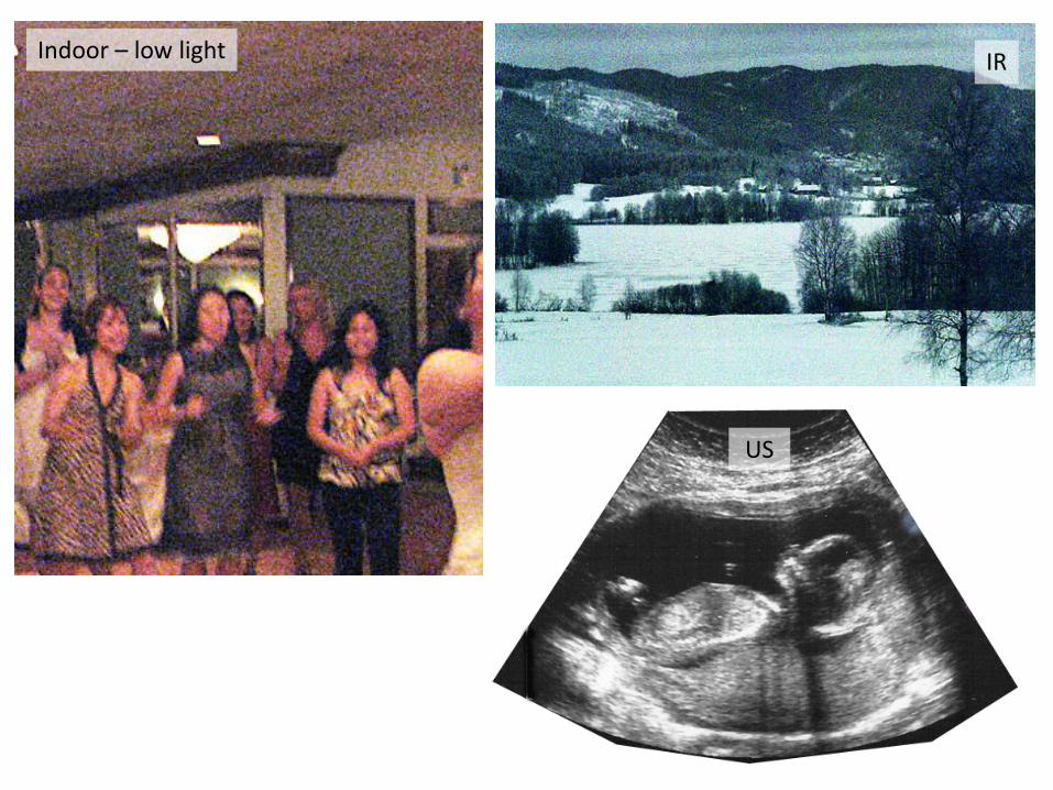
IRIndoor – low light

US

Sources of Noise

01010101010101010101010101010101010101010101010101

Multiplicative Noise(shot noise)

Additive Noise(read+amplifier noise)

Gain

�𝑥𝑥

Problem Definition

𝑥𝑥

𝑛𝑛

𝑦𝑦 = 𝑥𝑥 + 𝑛𝑛

Visual Quality

MSE / PSNR

�𝑛𝑛 = 𝑦𝑦 − �𝑥𝑥Noise?

Mean Square ErrorMSE = �𝑥𝑥 − 𝑥𝑥 2

2

Peak Signal-to-Noise ratio

PSNR = 20𝑙𝑙𝑙𝑙𝑙𝑙10255MSE

Outline

• Classical Denoising– Spatial Methods– Transform Methods

• State-of-the-art Methods– GSM – Gaussian Scale Mixture– NLM – Non-local means– BM3D – Block Matching 3D collaborative filtering

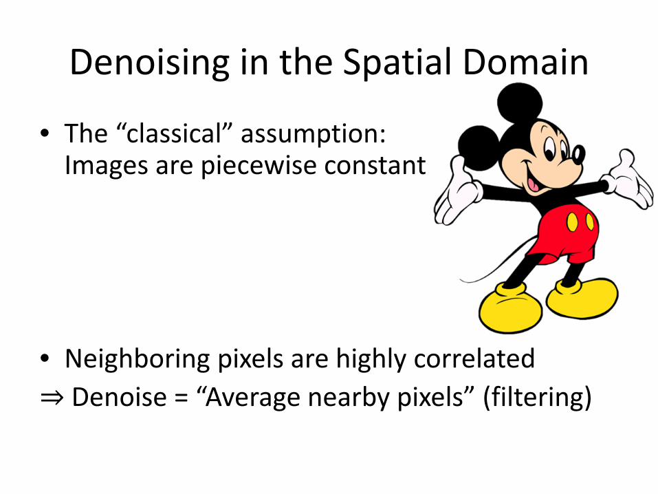
Denoising in the Spatial Domain

• The “classical” assumption:Images are piecewise constant

• Neighboring pixels are highly correlated⇒ Denoise = “Average nearby pixels” (filtering)

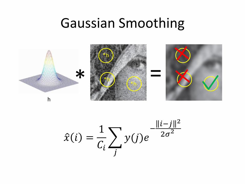
Gaussian Smoothing

* =*h

*h*h

h

�𝑥𝑥 𝑖𝑖 =1𝐶𝐶𝑖𝑖�𝑗𝑗

𝑦𝑦(𝑗𝑗)𝑒𝑒− 𝑖𝑖−𝑗𝑗 2

2𝜎𝜎2

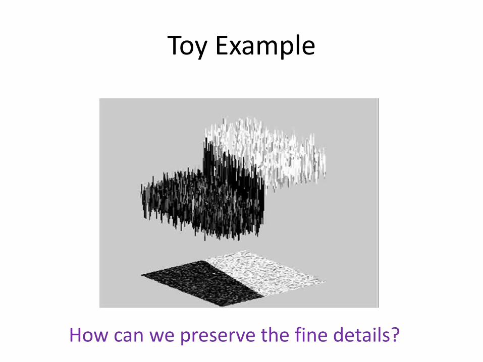
Toy Example

How can we preserve the fine details?

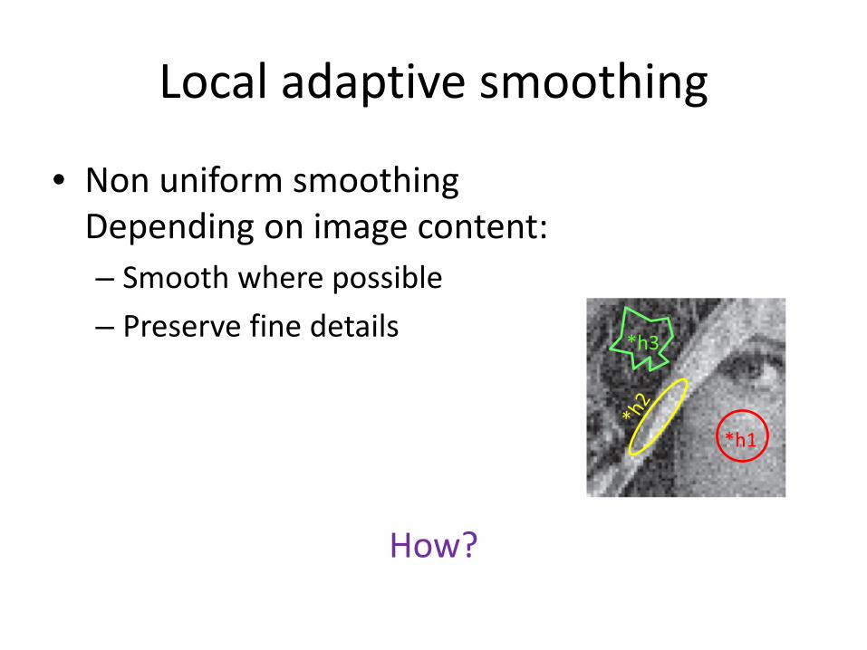
Local adaptive smoothing

• Non uniform smoothingDepending on image content: – Smooth where possible– Preserve fine details

How?

*h1

*h3

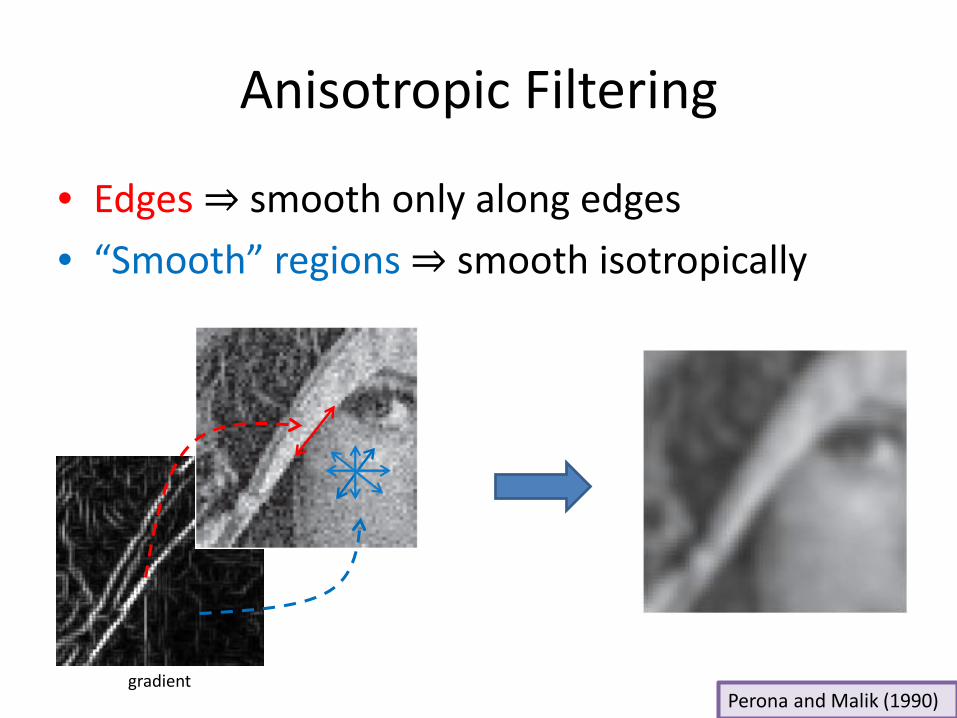
Anisotropic Filtering

• Edges ⇒ smooth only along edges• “Smooth” regions ⇒ smooth isotropically

gradientPerona and Malik (1990)

𝜌𝜌

𝜎𝜎

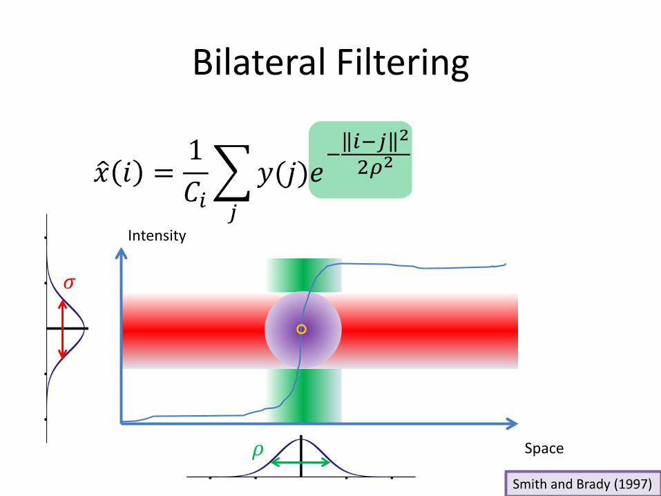
Bilateral Filtering

Space

Intensity

Smith and Brady (1997)

�𝑥𝑥 𝑖𝑖 =1𝐶𝐶𝑖𝑖�𝑗𝑗

𝑦𝑦(𝑗𝑗)𝑒𝑒− 𝑖𝑖−𝑗𝑗 2

2𝜌𝜌2 𝑒𝑒− 𝑦𝑦 𝑖𝑖 −𝑦𝑦(𝑗𝑗) 2

2𝜎𝜎2

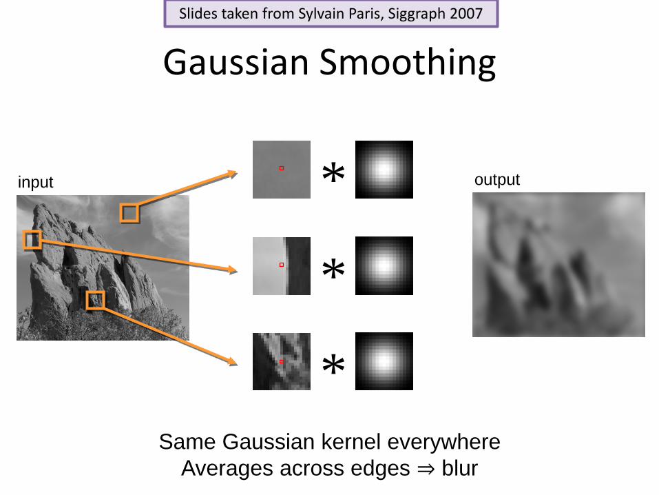
Gaussian Smoothing

*

*

*

input output

Same Gaussian kernel everywhereAverages across edges ⇒ blur

Slides taken from Sylvain Paris, Siggraph 2007

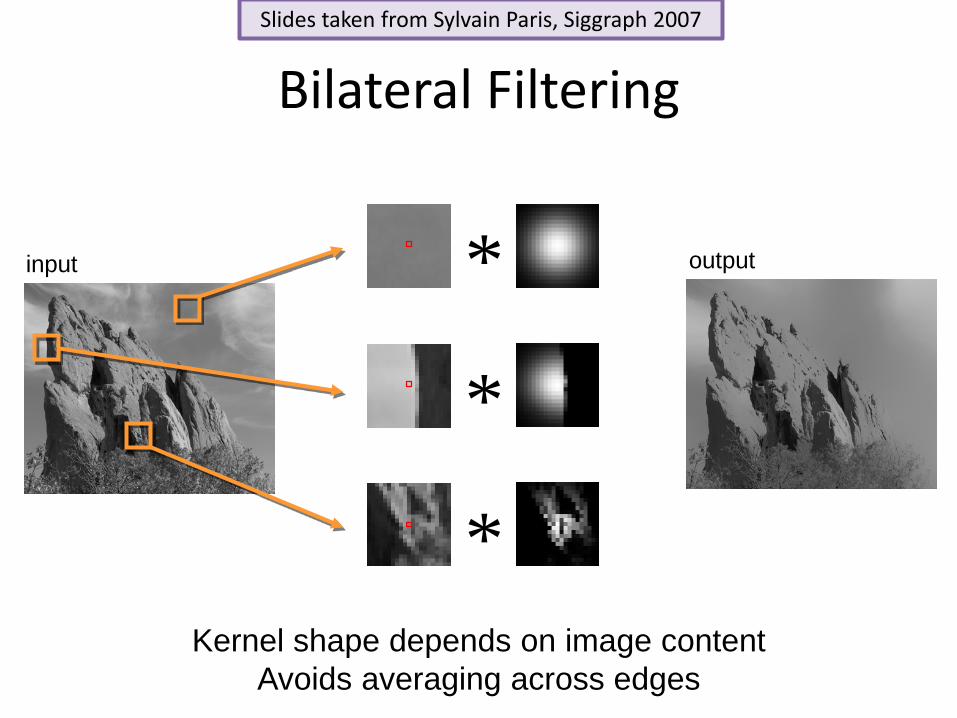
Bilateral Filtering

*

*

*

input output

Kernel shape depends on image contentAvoids averaging across edges

Slides taken from Sylvain Paris, Siggraph 2007

Denoising in the Transform Domain

• Motivation – New representation where signal and noise are more separated

• Denoise = “Suppress noise coefficients while preserving the signal coefficients”

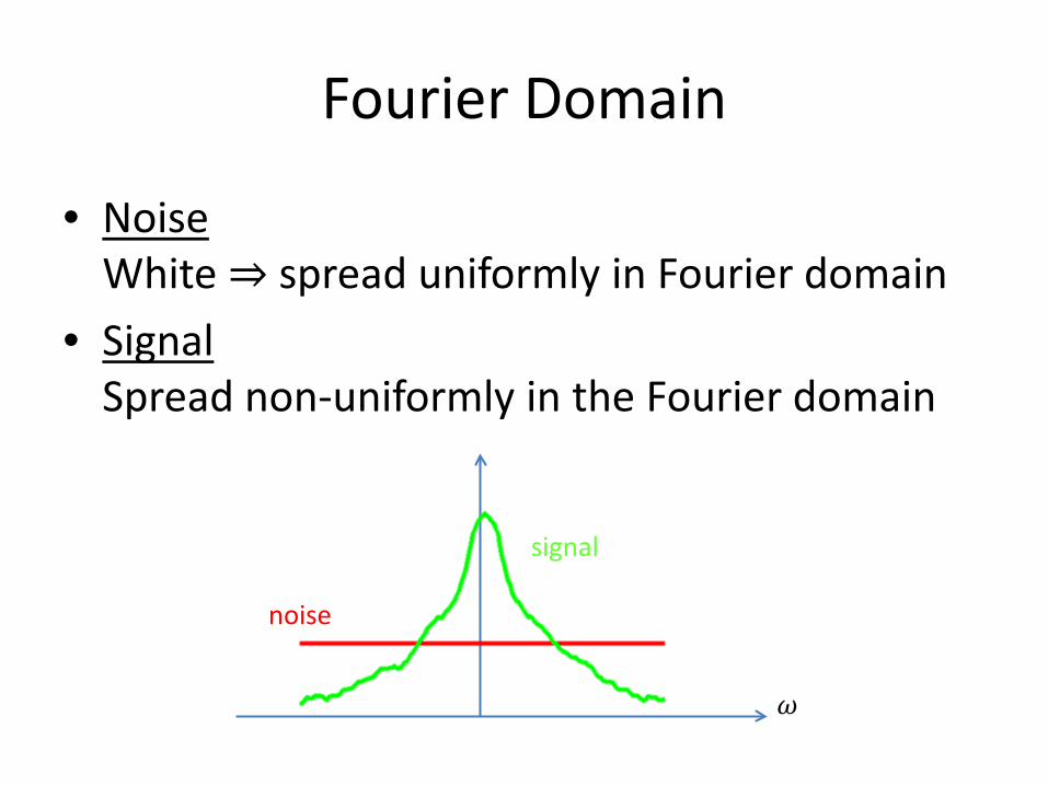
Fourier Domain

• Noise White ⇒ spread uniformly in Fourier domain

• SignalSpread non-uniformly in the Fourier domain

𝜔𝜔

signal

noise

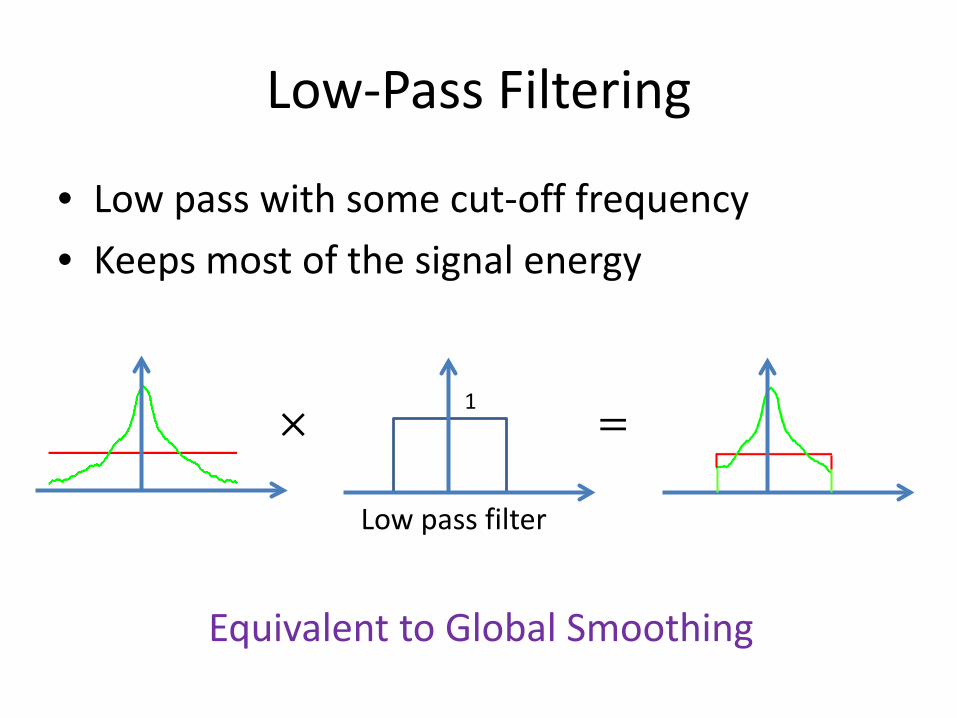
Low-Pass Filtering

• Low pass with some cut-off frequency• Keeps most of the signal energy

Equivalent to Global Smoothing

1× =

Low pass filter

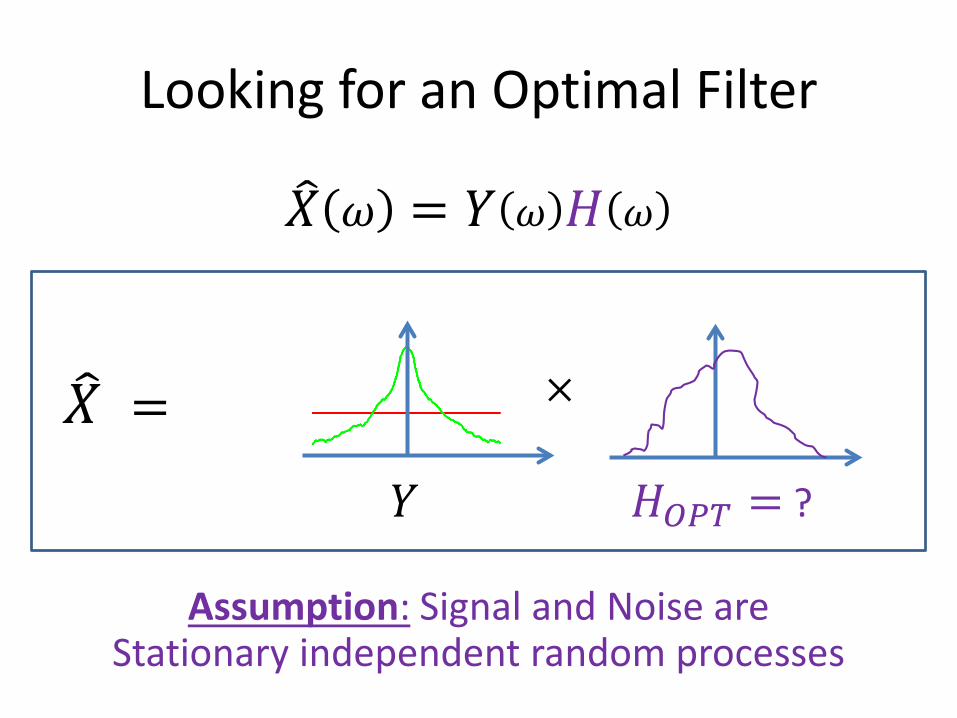
Looking for an Optimal Filter

�𝑋𝑋 𝜔𝜔 = 𝑌𝑌 𝜔𝜔 𝐻𝐻 𝜔𝜔

Assumption: Signal and Noise areStationary independent random processes

×

𝐻𝐻𝑂𝑂𝑂𝑂𝑂𝑂 = ?𝑌𝑌

�𝑋𝑋 =

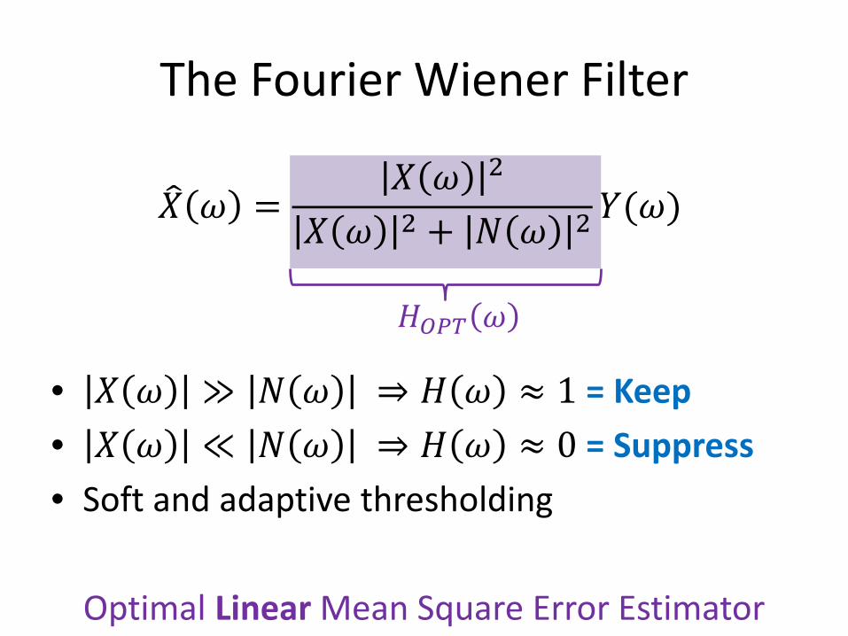
The Fourier Wiener Filter

�𝑋𝑋 𝜔𝜔 =𝑋𝑋 𝜔𝜔 2

𝑋𝑋 𝜔𝜔 2 + 𝑁𝑁 𝜔𝜔 2 𝑌𝑌(𝜔𝜔)

• 𝑋𝑋 𝜔𝜔 ≫ 𝑁𝑁 𝜔𝜔 ⇒ 𝐻𝐻 𝜔𝜔 ≈ 1 = Keep• 𝑋𝑋 𝜔𝜔 ≪ 𝑁𝑁 𝜔𝜔 ⇒ 𝐻𝐻 𝜔𝜔 ≈ 0 = Suppress• Soft and adaptive thresholding

Optimal Linear Mean Square Error Estimator

𝐻𝐻𝑂𝑂𝑂𝑂𝑂𝑂 𝜔𝜔

Fourier Wiener Filter in Practice

• Use a model for 𝑋𝑋 𝜔𝜔 2 - for example:

• Use 𝑌𝑌 𝜔𝜔 2 instead (empirical approach)

𝑋𝑋 𝜔𝜔 2 = 𝑙𝑙 𝑌𝑌 𝜔𝜔 2

or 𝑋𝑋 𝜔𝜔 2 = 𝐴𝐴(𝛼𝛼2+ 𝜔𝜔 2)1+𝜂𝜂

Ramani et al. (2006)“… the Stochastic Matern Model”

Why isn’t it enough?

• We assumed stationarity:“statistics of all image windows is the same”

• But natural images are not stationary

Why isn’t it enough?

• Mismatches and errors ⇒ global artifacts

The Windowed Fourier Wiener Filter

• Image has a local structure⇒ Denoise each region based on its own statistics

Perform Wiener filtering in image windows

Can we do better?

• Why restrict ourselves to a Fourier basis?• Other representations can be better:

– Sparsity ⇒ Signal/Noise separation– Localization of image details

Wavelets

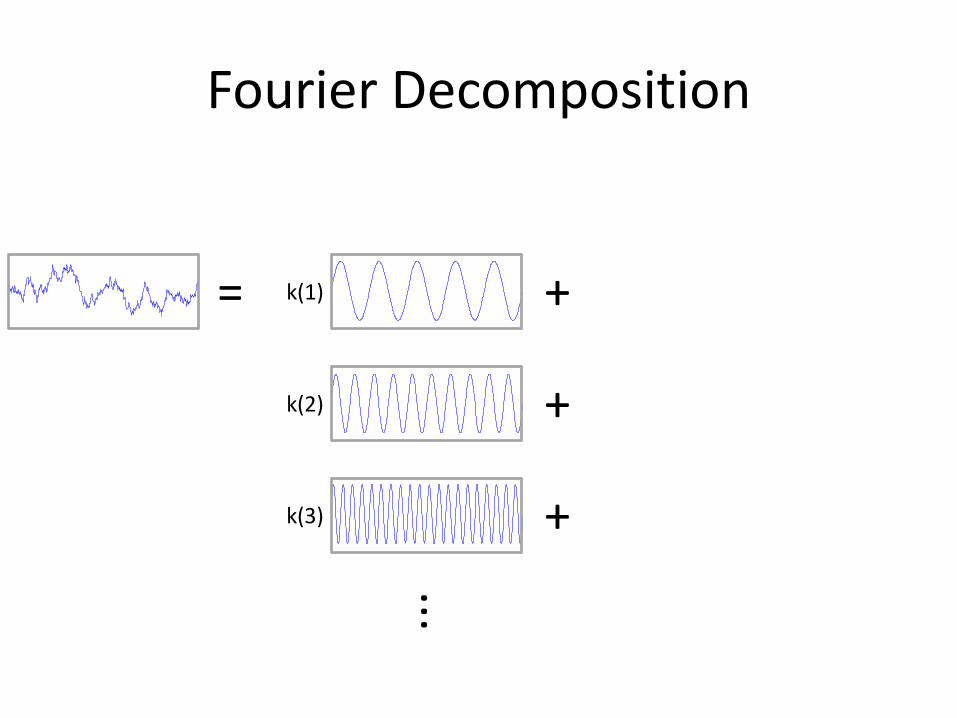
Fourier Decomposition

k(1) +=

k(2) +

k(3) +···

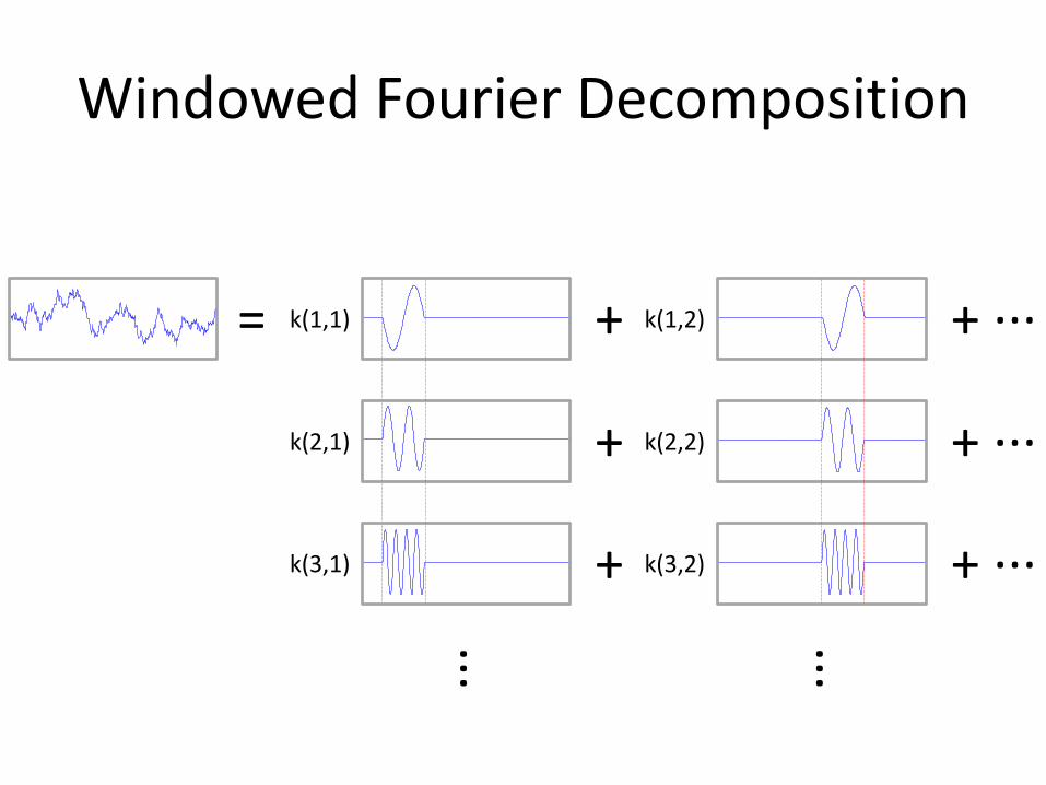
Windowed Fourier Decomposition

k(1,1) + k(1,2) + ···=

k(2,1) + k(2,2) + ···

k(3,1) + k(3,2) + ······ ···

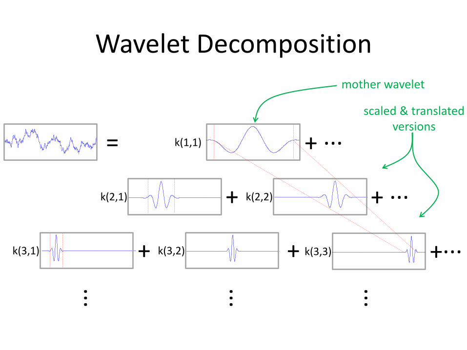
Wavelet Decomposition

k(1,1)

+ ···

=

k(3,3) +······ ···

k(3,2) +k(3,1) +

k(2,2)k(2,1) +

+ ···

···

mother wavelet

scaled & translatedversions

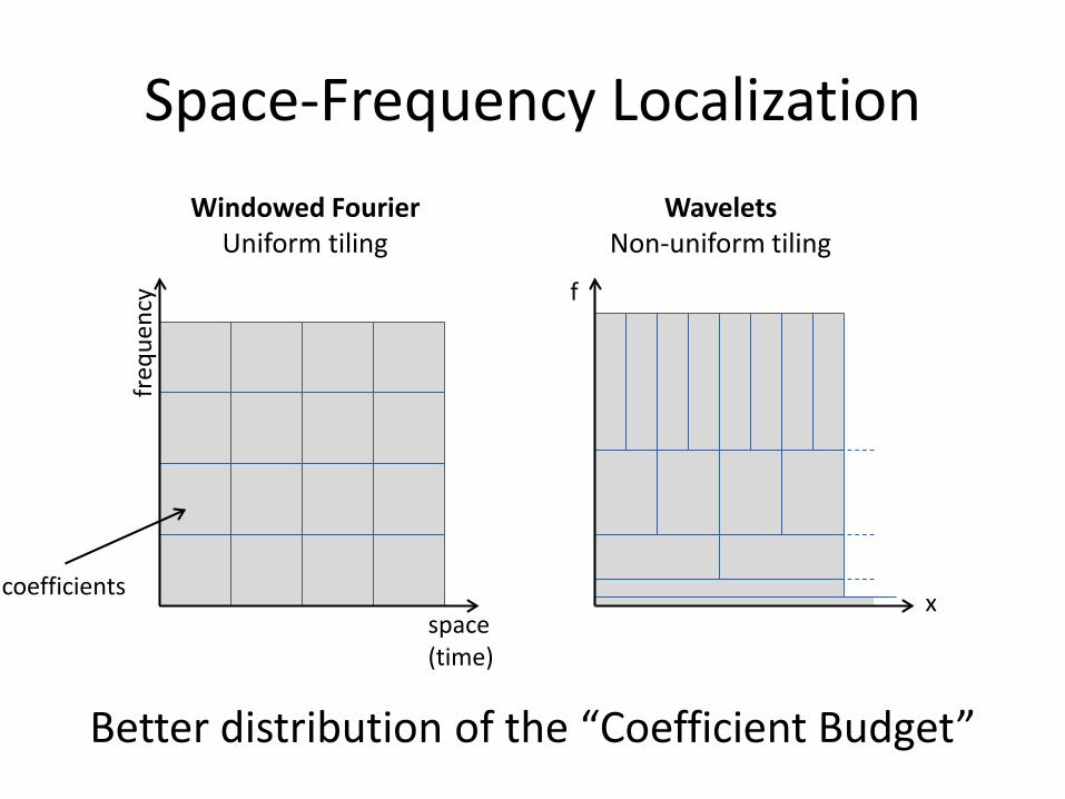
Space-Frequency Localization

Better distribution of the “Coefficient Budget”

f

x

freq

uenc

y

space(time)

Windowed FourierUniform tiling

WaveletsNon-uniform tiling

coefficients

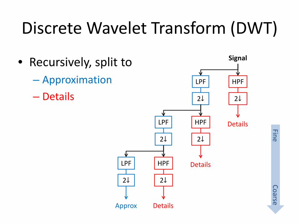
Discrete Wavelet Transform (DWT)

• Recursively, split to– Approximation– Details

Signal

HPFLPF

2↓2↓

DetailsHPFLPF

2↓2↓

DetailsHPFLPF

2↓2↓

DetailsApprox

Fine Coarse

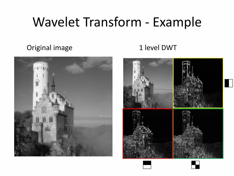
Wavelet Transform - Example

Original image 1 level DWT

Wavelet Transform - Example

2 level DWTOriginal image

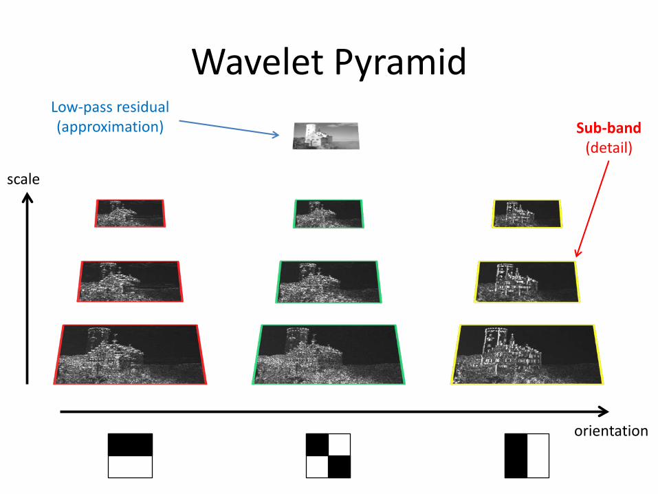
Wavelet PyramidLow-pass residual(approximation) Sub-band

(detail)

scale

orientation

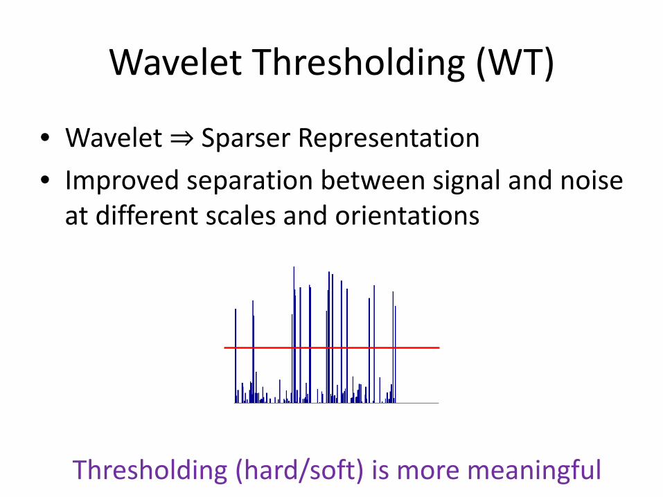
Wavelet Thresholding (WT)

• Wavelet ⇒ Sparser Representation• Improved separation between signal and noise

at different scales and orientations

Thresholding (hard/soft) is more meaningful

A Probabilistic Perspective

• Learn or assume statistical model of image and noise - 𝑝𝑝 𝑥𝑥 ,𝑝𝑝 𝑛𝑛

• Use Bayesian inference to obtain �𝑥𝑥

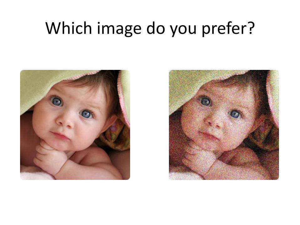
Which image do you prefer?

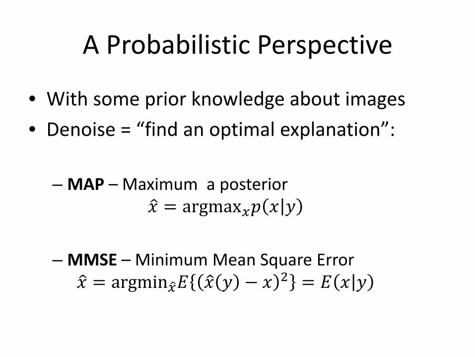
A Probabilistic Perspective

• With some prior knowledge about images• Denoise = “find an optimal explanation”:

– MAP – Maximum a posterior�𝑥𝑥 = argmax𝑥𝑥𝑝𝑝 𝑥𝑥 𝑦𝑦

– MMSE – Minimum Mean Square Error�𝑥𝑥 = argmin �𝑥𝑥𝐸𝐸 �𝑥𝑥 𝑦𝑦 − 𝑥𝑥 2 = 𝐸𝐸 𝑥𝑥 𝑦𝑦

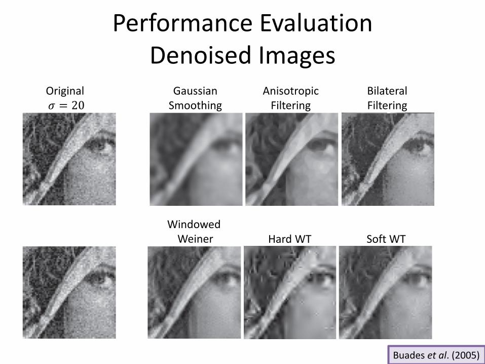
Performance Evaluation Denoised Images

Buades et al. (2005)

WindowedWeiner Hard WT Soft WT

GaussianSmoothing

Anisotropic Filtering

Bilateral Filtering

Original 𝜎𝜎 = 20

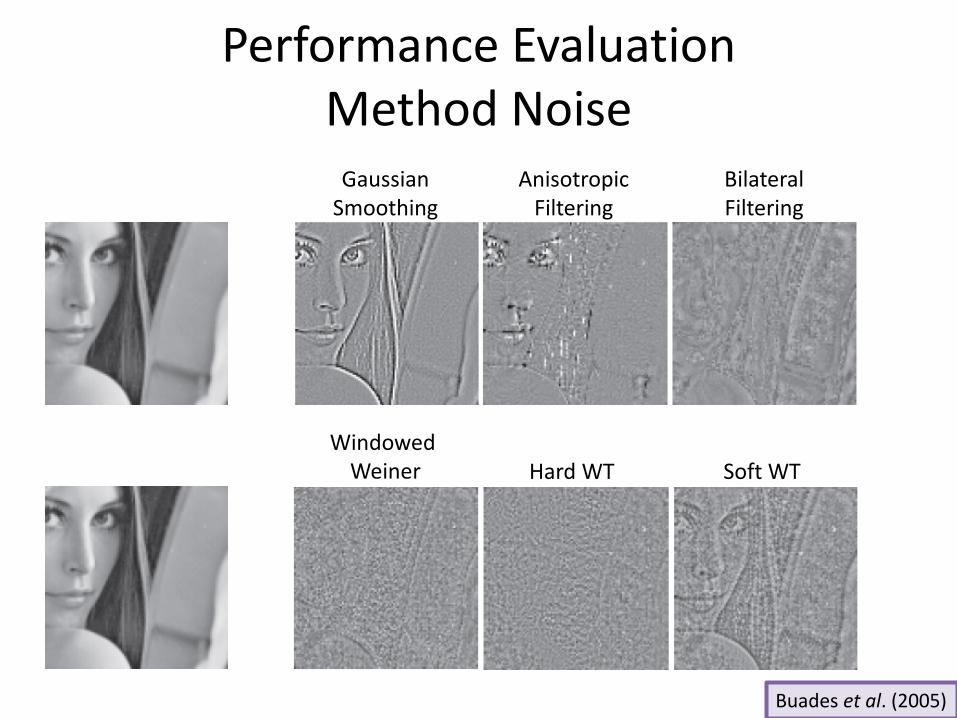
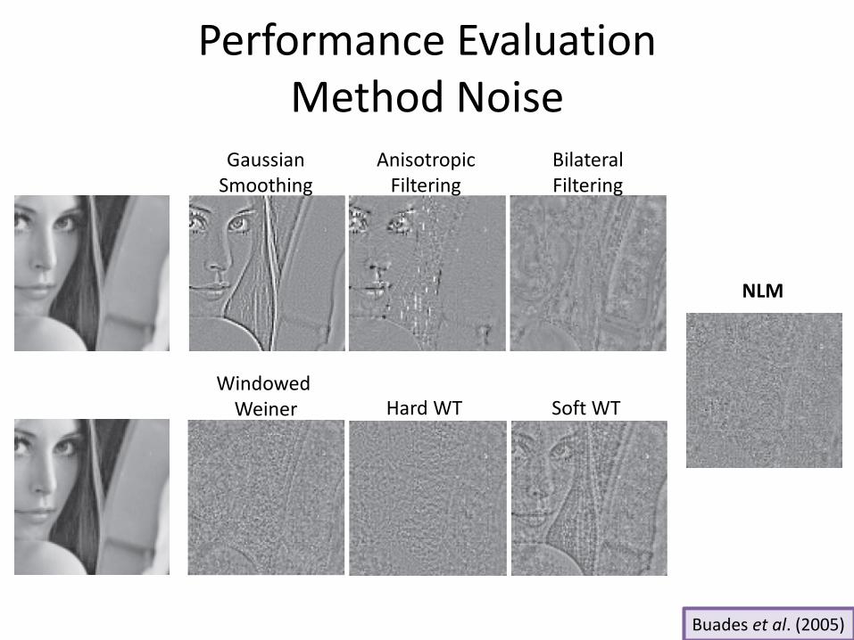
Performance Evaluation Method Noise

Buades et al. (2005)

WindowedWeiner Hard WT Soft WT

GaussianSmoothing

Anisotropic Filtering

Bilateral Filtering

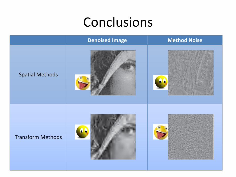
ConclusionsDenoised Image Method Noise

Spatial Methods

Transform Methods

Taking it up a notch...

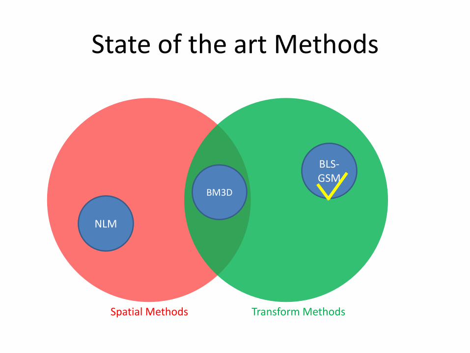
State of the art Methods

BLS-GSM

NLM

BM3D

Spatial Methods Transform Methods

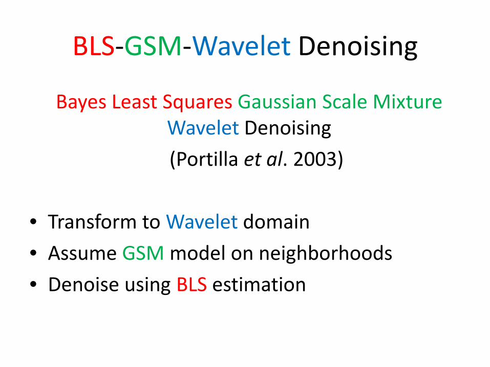
BLS-GSM-Wavelet Denoising

Bayes Least Squares Gaussian Scale MixtureWavelet Denoising(Portilla et al. 2003)

• Transform to Wavelet domain• Assume GSM model on neighborhoods• Denoise using BLS estimation

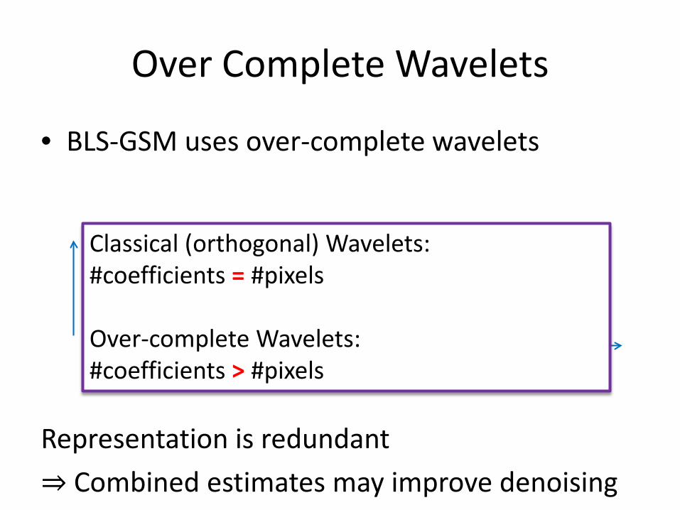
• BLS-GSM uses over-complete wavelets

Representation is redundant⇒ Combined estimates may improve denoising

Over Complete Wavelets

…Classical (orthogonal) Wavelets:#coefficients = #pixels

Over-complete Wavelets:#coefficients > #pixels

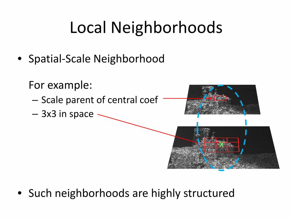
Local Neighborhoods

• Spatial-Scale Neighborhood

For example:– Scale parent of central coef– 3x3 in space

• Such neighborhoods are highly structured

x

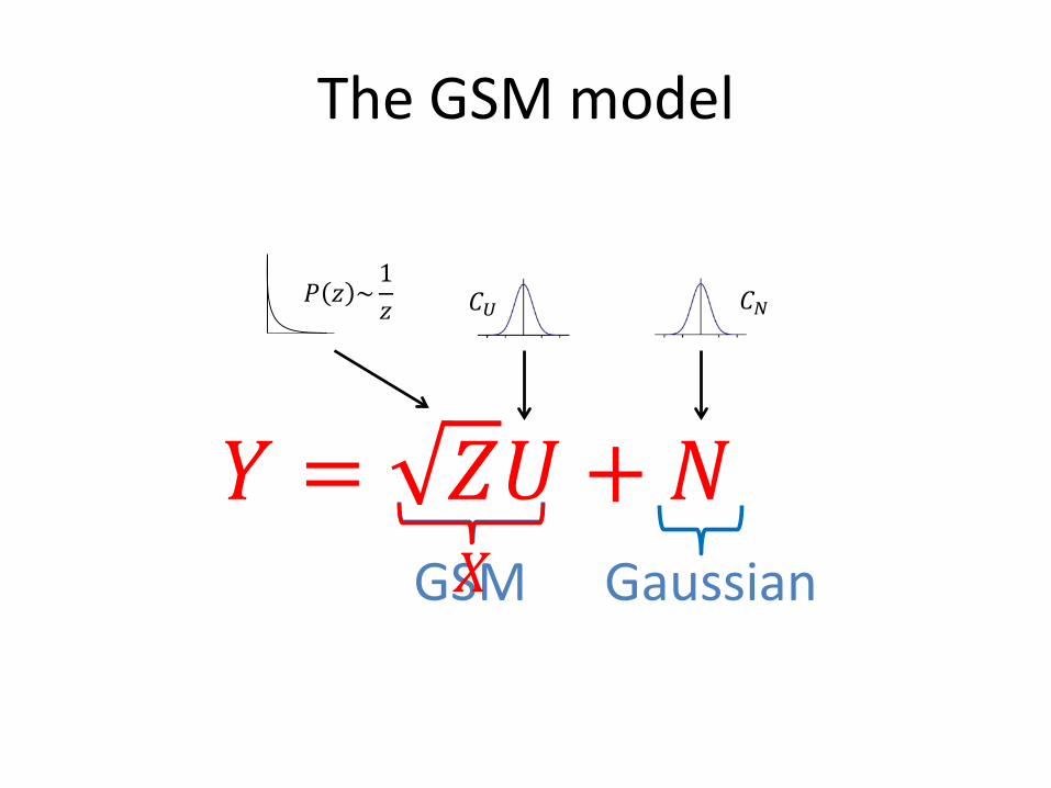
The GSM model

𝑌𝑌 = 𝑍𝑍𝑈𝑈 + 𝑁𝑁GSM

𝐶𝐶𝑈𝑈𝑃𝑃 𝑧𝑧 ~1𝑧𝑧 𝐶𝐶𝑁𝑁

Gaussian𝑋𝑋

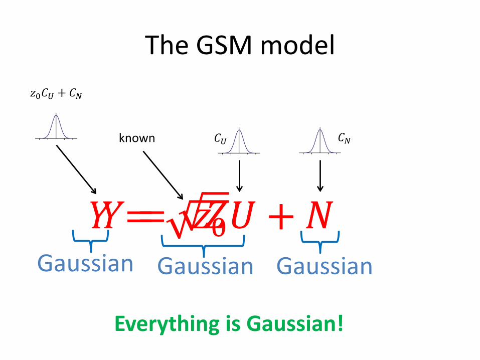
The GSM model

𝑌𝑌 = 𝑍𝑍𝑈𝑈 + 𝑁𝑁

𝐶𝐶𝑈𝑈 𝐶𝐶𝑁𝑁

GaussianGaussian

𝑌𝑌 = 𝑧𝑧0𝑈𝑈 + 𝑁𝑁

known

𝑧𝑧0𝐶𝐶𝑈𝑈 + 𝐶𝐶𝑁𝑁

Gaussian

Everything is Gaussian!

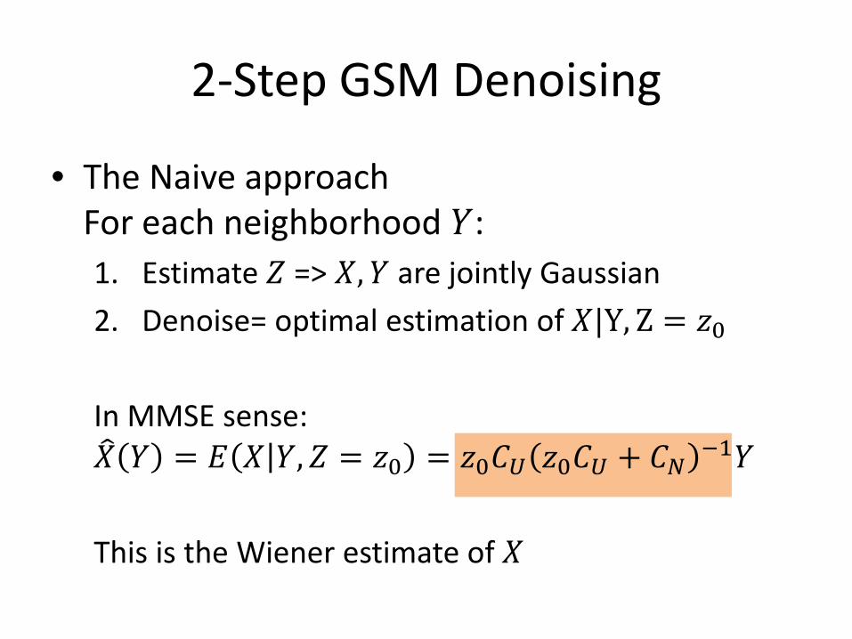
2-Step GSM Denoising

• The Naive approachFor each neighborhood 𝑌𝑌:1. Estimate 𝑍𝑍 => 𝑋𝑋,𝑌𝑌 are jointly Gaussian2. Denoise= optimal estimation of 𝑋𝑋|Y, Z = 𝑧𝑧0

In MMSE sense:�𝑋𝑋 𝑌𝑌 = 𝐸𝐸 𝑋𝑋 𝑌𝑌,𝑍𝑍 = 𝑧𝑧0 = 𝑧𝑧0𝐶𝐶𝑈𝑈 𝑧𝑧0𝐶𝐶𝑈𝑈 + 𝐶𝐶𝑁𝑁 −1𝑌𝑌

This is the Wiener estimate of 𝑋𝑋

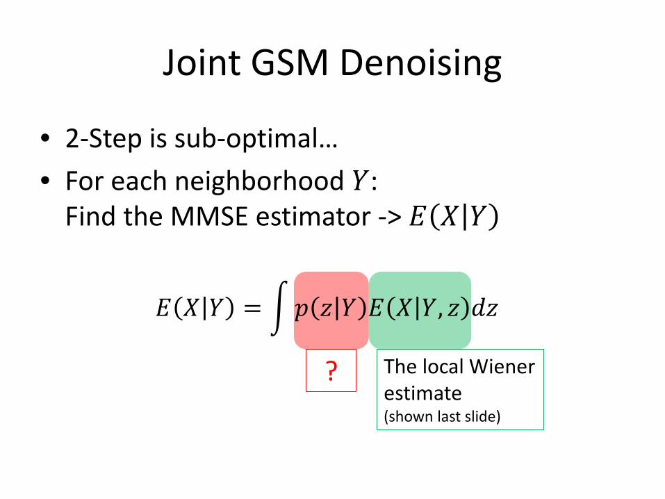
Joint GSM Denoising

The local Wiener estimate (shown last slide)

?

• 2-Step is sub-optimal…• For each neighborhood 𝑌𝑌:

Find the MMSE estimator -> 𝐸𝐸 𝑋𝑋 𝑌𝑌

𝐸𝐸 𝑋𝑋 𝑌𝑌 = �𝑝𝑝 𝑧𝑧 𝑌𝑌 𝐸𝐸 𝑋𝑋 𝑌𝑌, 𝑧𝑧 𝑑𝑑𝑧𝑧

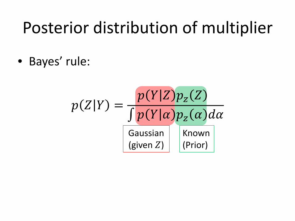
• Bayes’ rule:

𝑝𝑝 𝑍𝑍 𝑌𝑌 =𝑝𝑝 𝑌𝑌 𝑍𝑍 𝑝𝑝𝑧𝑧 𝑍𝑍

∫𝑝𝑝 𝑌𝑌 𝛼𝛼 𝑝𝑝𝑧𝑧 𝛼𝛼 𝑑𝑑𝛼𝛼

Posterior distribution of multiplier

Known(Prior)

Gaussian(given 𝑍𝑍)

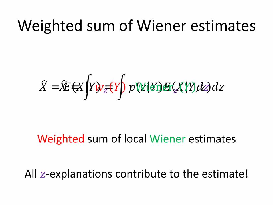
Weighted sum of Wiener estimates

Weighted sum of local Wiener estimates

All 𝑧𝑧-explanations contribute to the estimate!

�𝑋𝑋 = 𝐸𝐸 𝑋𝑋 𝑌𝑌 = �𝑝𝑝 𝑧𝑧 𝑌𝑌 𝐸𝐸 𝑋𝑋 𝑌𝑌, 𝑧𝑧 𝑑𝑑𝑧𝑧�𝑋𝑋 = �𝑤𝑤𝑧𝑧 𝑌𝑌 � Wiener𝑧𝑧 𝑌𝑌 𝑑𝑑𝑧𝑧

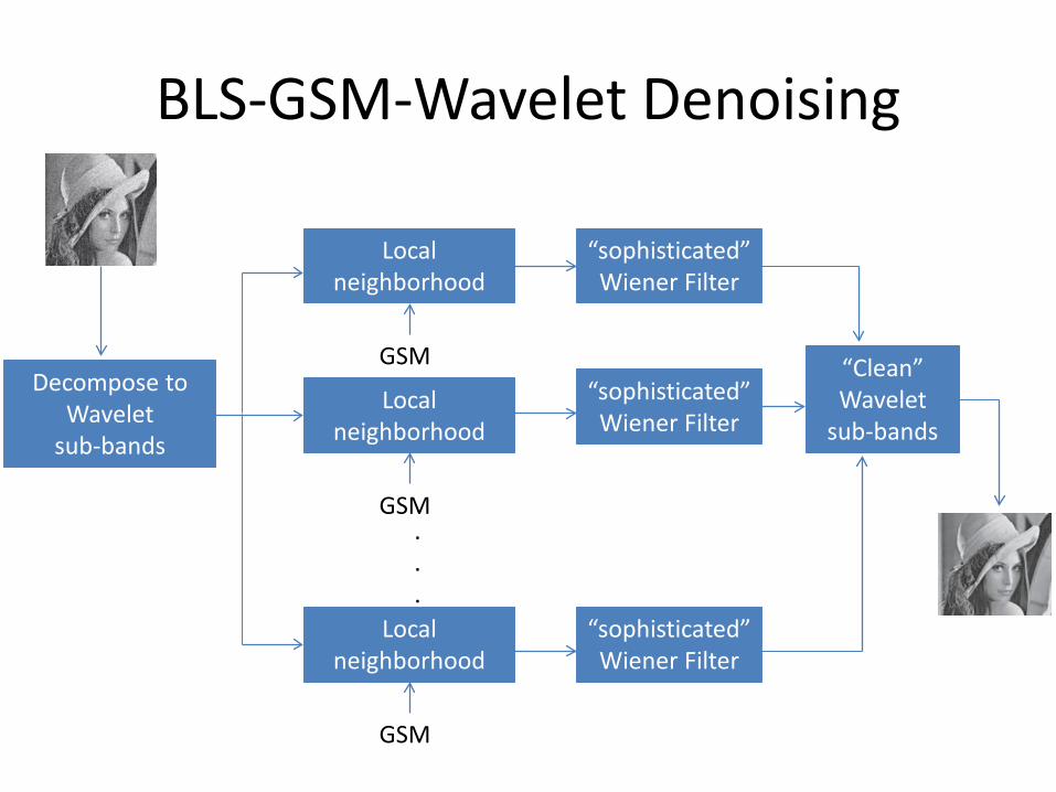
BLS-GSM-Wavelet Denoising

Decompose toWavelet

sub-bands

.

.

.Local

neighborhood

GSM

Local neighborhood

GSM

Local neighborhood

GSM

“sophisticated” Wiener Filter

“sophisticated” Wiener Filter

“sophisticated” Wiener Filter

“Clean” Wavelet

sub-bands

State of the art Methods

BLS-GSM

NLM

BM3D

Spatial Methods Transform Methods

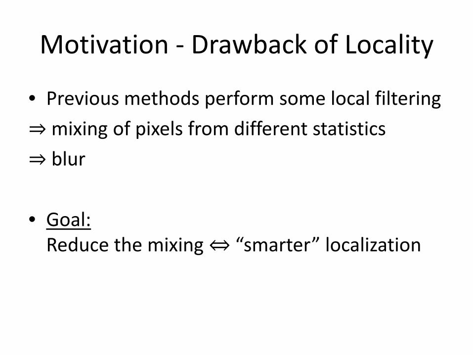
Motivation - Drawback of Locality

• Previous methods perform some local filtering⇒ mixing of pixels from different statistics⇒ blur

• Goal:Reduce the mixing ⇔ “smarter” localization

Motivation - Temporal perspective

• Assume a static scene• Consider multiple images y(𝑡𝑡) at different times• The signal 𝑥𝑥(𝑡𝑡) remains constant• 𝑛𝑛(𝑡𝑡) varies over time with zero mean

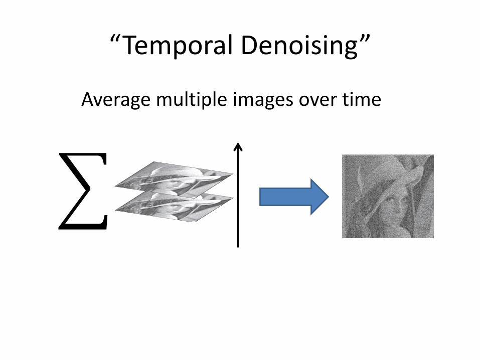
“Temporal Denoising”

�

Average multiple images over time

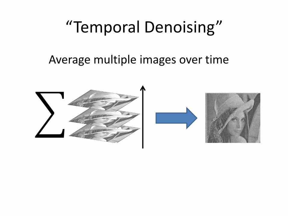
“Temporal Denoising”

�

Average multiple images over time

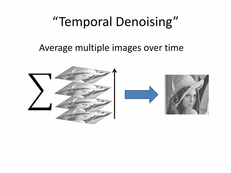
“Temporal Denoising”

�

Average multiple images over time

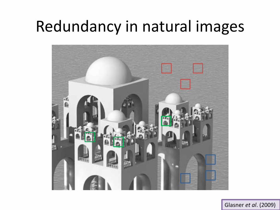
Redundancy in natural images

Glasner et al. (2009)

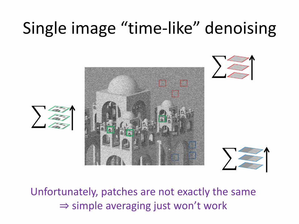
Single image “time-like” denoising

�

�

�

Unfortunately, patches are not exactly the same ⇒ simple averaging just won’t work

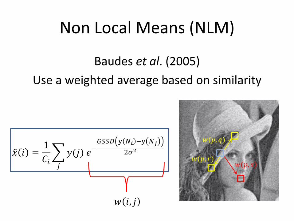
Non Local Means (NLM)

Baudes et al. (2005)Use a weighted average based on similarity

𝑤𝑤(𝑝𝑝, 𝑞𝑞)

𝑤𝑤(𝑝𝑝, 𝑟𝑟)𝑤𝑤(𝑝𝑝, 𝑠𝑠)

�𝑥𝑥 𝑖𝑖 =1𝐶𝐶𝑖𝑖�𝑗𝑗

𝑦𝑦(𝑗𝑗) 𝑒𝑒−𝐺𝐺𝑆𝑆𝑆𝑆𝑆𝑆 y 𝑁𝑁𝑖𝑖 −y 𝑁𝑁𝑗𝑗

2𝜎𝜎2

𝑤𝑤 𝑖𝑖, 𝑗𝑗

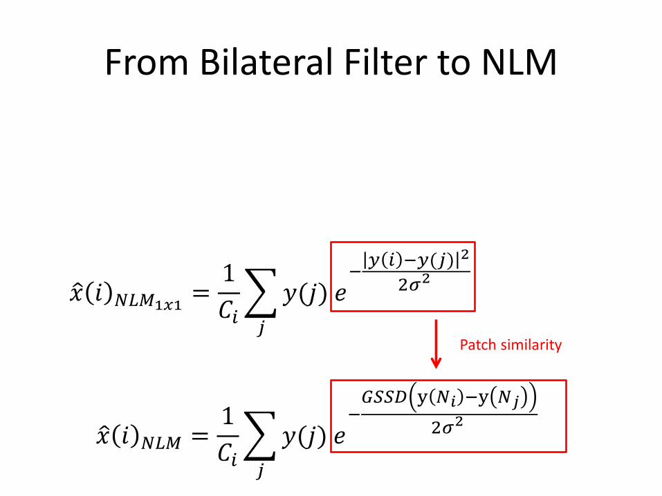
From Bilateral Filter to NLM

�𝑥𝑥 𝑖𝑖 𝐵𝐵𝐵𝐵 =1𝐶𝐶𝑖𝑖�𝑗𝑗

𝑦𝑦(𝑗𝑗)𝑒𝑒− 𝑦𝑦 𝑖𝑖 −𝑦𝑦(𝑗𝑗) 2

2𝜎𝜎2 𝑒𝑒− 𝑖𝑖−𝑗𝑗 2

2𝜌𝜌2

�𝑥𝑥 𝑖𝑖 𝑁𝑁𝐵𝐵𝑁𝑁1𝑥𝑥1 =1𝐶𝐶𝑖𝑖�𝑗𝑗

𝑦𝑦(𝑗𝑗) 𝑒𝑒− 𝑦𝑦 𝑖𝑖 −𝑦𝑦(𝑗𝑗) 2

2𝜎𝜎2

𝜌𝜌 → ∞intensity weight spatial weight

From Bilateral Filter to NLM

�𝑥𝑥 𝑖𝑖 𝑁𝑁𝐵𝐵𝑁𝑁1𝑥𝑥1 =1𝐶𝐶𝑖𝑖�𝑗𝑗

𝑦𝑦(𝑗𝑗) 𝑒𝑒− 𝑦𝑦 𝑖𝑖 −𝑦𝑦(𝑗𝑗) 2

2𝜎𝜎2

�𝑥𝑥 𝑖𝑖 𝑁𝑁𝐵𝐵𝑁𝑁 =1𝐶𝐶𝑖𝑖�𝑗𝑗

𝑦𝑦(𝑗𝑗) 𝑒𝑒−𝐺𝐺𝑆𝑆𝑆𝑆𝑆𝑆 y 𝑁𝑁𝑖𝑖 −y 𝑁𝑁𝑗𝑗

2𝜎𝜎2

Patch similarity

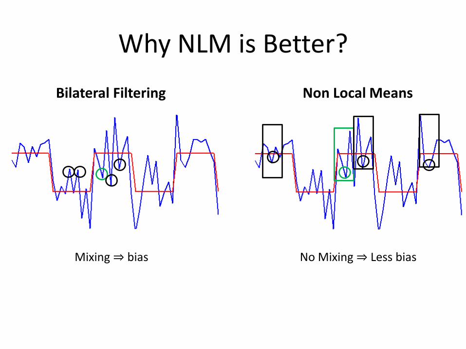
Why NLM is Better?

Mixing ⇒ bias No Mixing ⇒ Less bias

Bilateral Filtering Non Local Means

Performance Evaluation Method Noise

Buades et al. (2005)

WindowedWeiner Hard WT Soft WT

GaussianSmoothing

Anisotropic Filtering

Bilateral Filtering

NLM

What’s Next?

• The idea of grouping sounds good⇒ reduces mixing

• Denoise = “extract the common (the signal)”

• NLM: common = weighted average• Can a sparser representation do better?

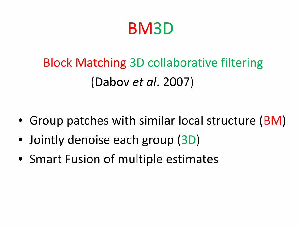
BM3D

Block Matching 3D collaborative filtering (Dabov et al. 2007)

• Group patches with similar local structure (BM)• Jointly denoise each group (3D)• Smart Fusion of multiple estimates

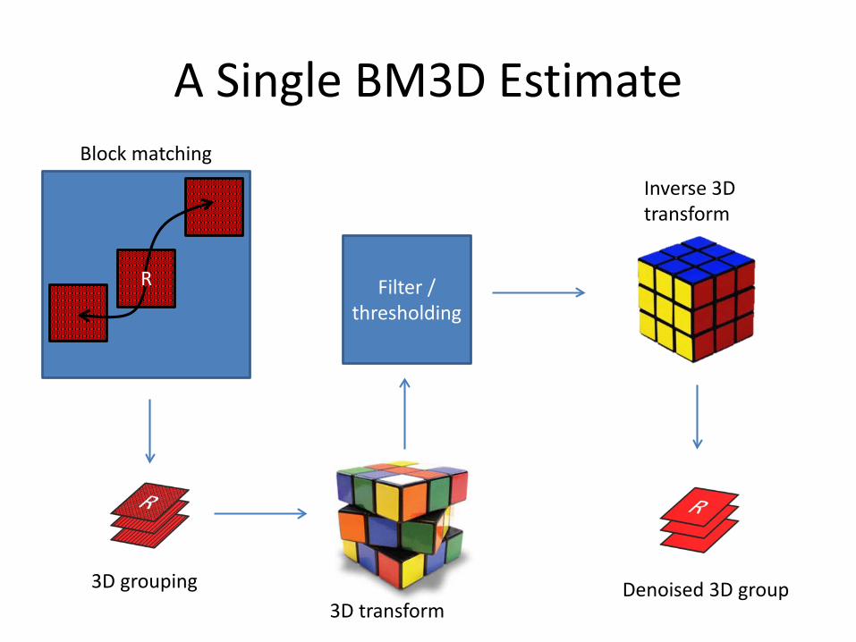
A Single BM3D Estimate

R

Block matching

3D grouping3D transform

Filter / thresholding

Inverse 3D transform

Denoised 3D group

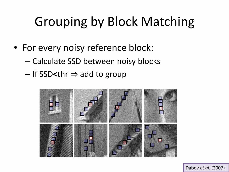
Grouping by Block Matching

• For every noisy reference block:– Calculate SSD between noisy blocks– If SSD<thr ⇒ add to group

Dabov et al. (2007)

3D Transform

Reminder:

2D transformSparisity

𝛼𝛼

𝑘𝑘𝛼𝛼

𝛼𝛼3D transform

2D transform

2D transform

BM3D approach:

naive approach:

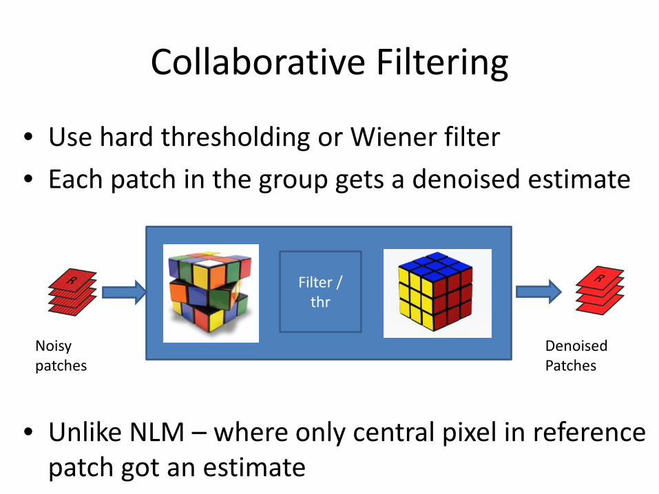
Collaborative Filtering

• Use hard thresholding or Wiener filter• Each patch in the group gets a denoised estimate

• Unlike NLM – where only central pixel in reference patch got an estimate

Filter / thr

DenoisedPatches

Noisy patches

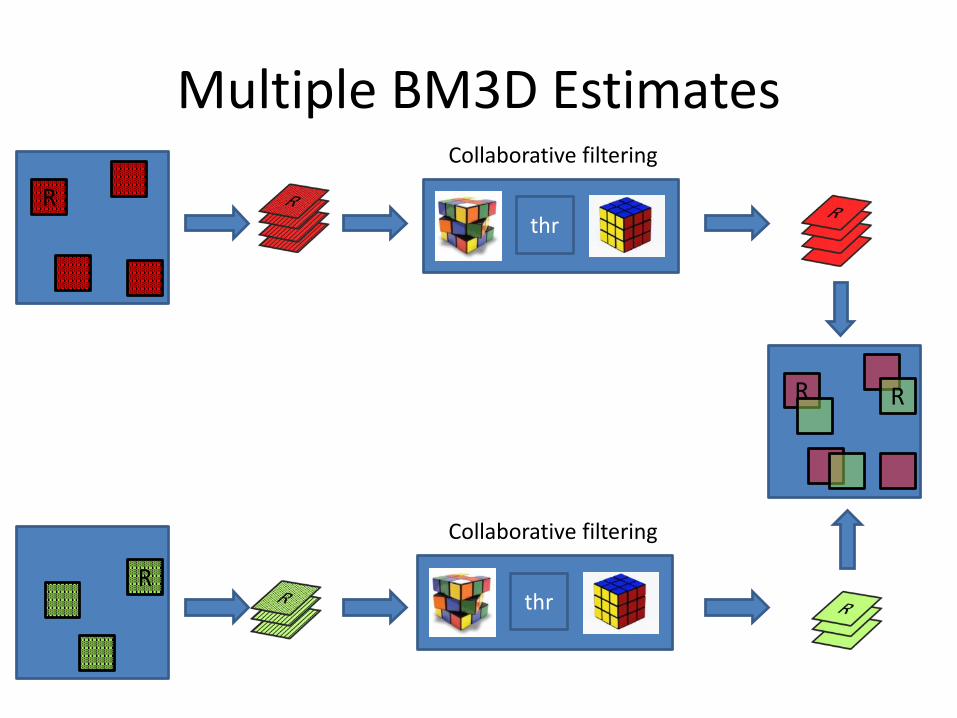
Multiple BM3D Estimates

R

thr

thr

R

R R

Collaborative filtering

Collaborative filtering

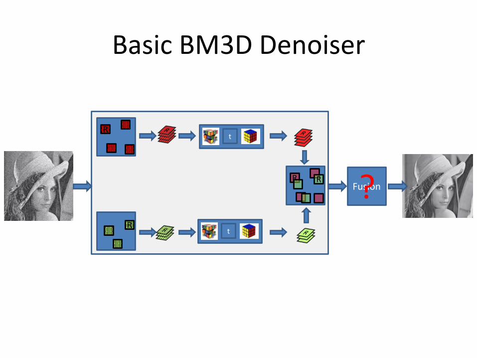
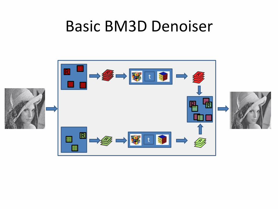
Basic BM3D Denoiser

R

t

t

R

R RFusion?

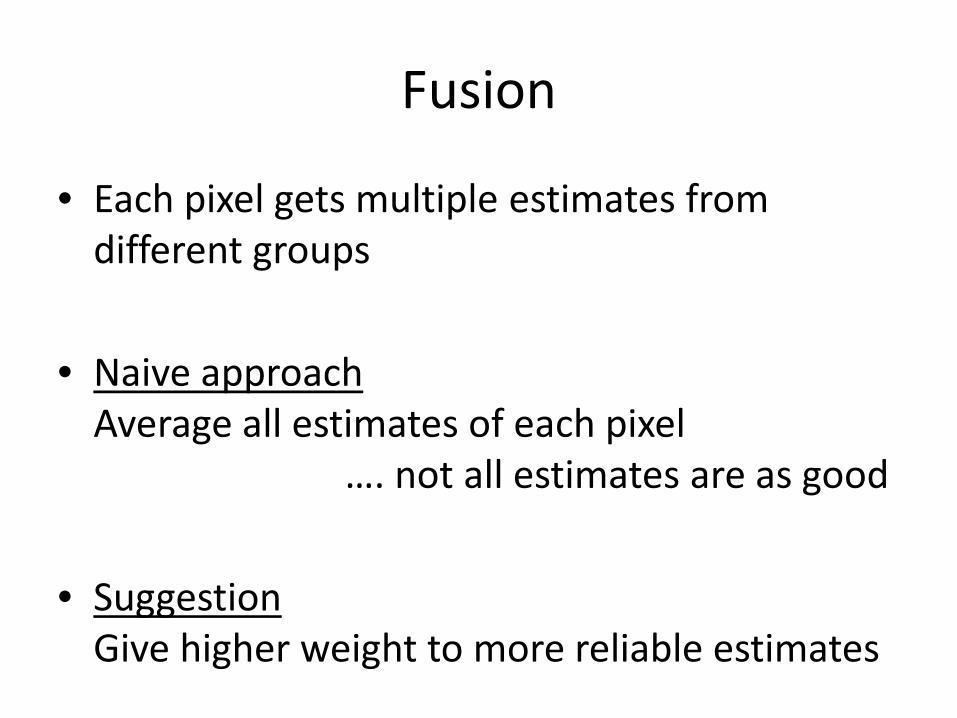
Fusion

• Each pixel gets multiple estimates from different groups

• Naive approach Average all estimates of each pixel

…. not all estimates are as good

• SuggestionGive higher weight to more reliable estimates

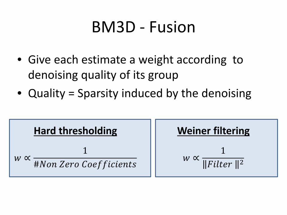
BM3D - Fusion

• Give each estimate a weight according to denoising quality of its group

• Quality = Sparsity induced by the denoising

Hard thresholding

𝑤𝑤 ∝1

#𝑁𝑁𝑙𝑙𝑛𝑛 𝑍𝑍𝑒𝑒𝑟𝑟𝑙𝑙 𝐶𝐶𝑙𝑙𝑒𝑒𝐶𝐶𝐶𝐶𝑖𝑖𝐶𝐶𝑖𝑖𝑒𝑒𝑛𝑛𝑡𝑡𝑠𝑠

Weiner filtering

𝑤𝑤 ∝1

𝐹𝐹𝑖𝑖𝑙𝑙𝑡𝑡𝑒𝑒𝑟𝑟 2

BM3D in Practice

• Noise may result in poor matching ⇒ Degrades de-noising performance

• Improvements:1. Match using a smoothed version of the image2. Perform BM3D in 2 phases:

a. Basic BM3D estimate ⇒ improved 3D groups b. Final BM3D

Basic BM3D Denoiser

R

t

t

R

R R

Two phase BM3D Denoising

R

t

t

R

R R

R

t

t

R

R R

(a)Basic denoising:

Hard thresholding

(b)Final denoising:Wiener filtering

Results and Comparison

• Comparison:– Different levels of noise– Different sets of images

• Evaluation methods:– MSE/PSNR– Visual comparison to noisy and/or original images

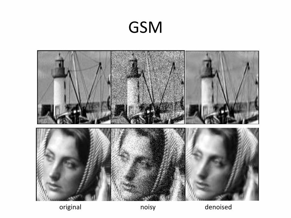
GSM

noisyoriginal denoised

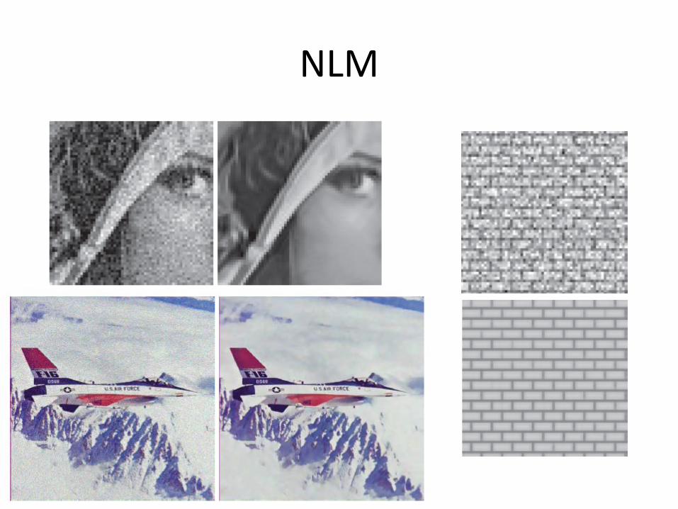
NLM

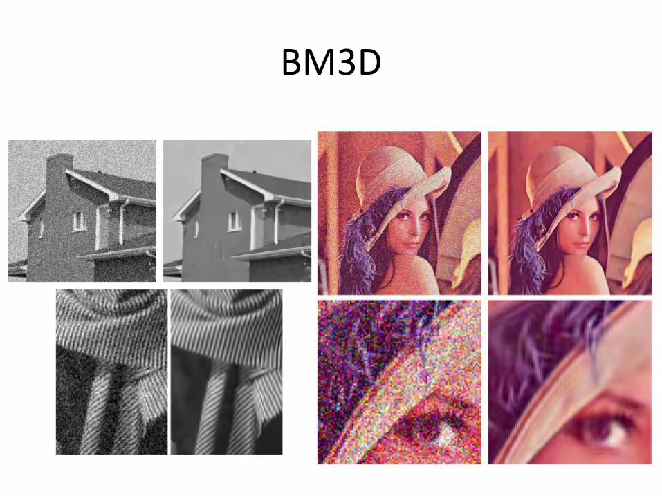
BM3D

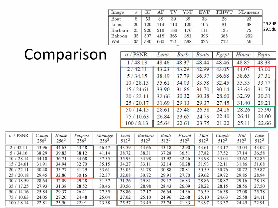
Comparison

29.8dB29.5dB

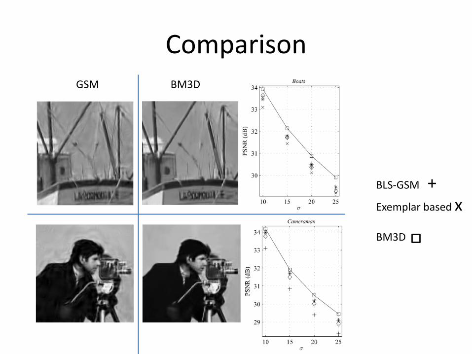
BLS-GSM +Exemplar based x

BM3D

ComparisonGSM BM3D

Comments

• Average improvement from naive Gaussian filtering to NLM – 4-5 dB

• Average improvement of 1 dB over 4 years (from BLS-GSM(2003) to BM3D(2007))

• Saturation in PSNR over the last 4 years (BM3D still considered state of the art)