electronics

Article

Indoor 3-D RT Radio Wave Propagation PredictionMethod: PL and RSSI Modeling Validation byMeasurement at 4.5 GHz

Ferdous Hossain 1,* , Tan Kim Geok 1,*, Tharek Abd Rahman 2, Mohammad Nour Hindia 3,

Kaharudin Dimyati 3, Sharif Ahmed 1, C. P. Tso 1 , Azlan Abdaziz 1, W. Lim 1, Azwan Mahmud 4,

Tan Choo Peng 5, Chia Pao Liew 6 and Vinesh Thiruchelvam 7

1 Faculty of Engineering and Technology, Multimedia University, Melaka 75450, Malaysia2 Faculty of Electrical Engineering, Universiti Teknologi Malaysia, Johor Bahru 81310, Malaysia3 Faculty of Engineering, Department of Electrical Engineering, University of Malaya,

Kuala Lumpur 50603, Malaysia4 Faculty of Engineering, Multimedia University, Cyberjaya 63100, Malaysia5 Faculty of Information Science and Technology, Multimedia University, Melaka 75450, Malaysia6 Faculty of Engineering and Technology, Tunku Abdul Rahman University College,

Kuala Lumpur 53300, Malaysia7 Faculty of Computing, Engineering and Technology, Asia Pacific University of Technology & Innovation,

Kuala Lumpur 57000, Malaysia

* Correspondence: ferdous.mbstu.cse@gmail.com (F.H.); kgtan@mmu.edu.my (T.K.G.);

Tel.: +60-112-108-6919 (F.H.); +60-013-613-6138 (T.K.G.)

Received: 10 May 2019; Accepted: 5 June 2019; Published: 3 July 2019�����������������

Abstract: This article introduces an efficient analysis of indoor 4.5 GHz radio wave propagation by

using a proposed three-dimensional (3-D) ray-tracing (RT) modeling and measurement. The attractive

facilities of this frequency band have significantly increased in indoor radio wave communication

systems. Radio propagation predictions by simulation method based on a site-specific model, such

as RT is widely used to categorize radio wave channels. Although practical measurement provides

accurate results, it still needs a considerable amount of resources. Hence, a computerized simulation

tool would be a good solution to categorize the wireless channels. The simulation has been performed

with an in-house developed software tool. Here, the 3-D shooting bouncing ray tracing (SBRT) and the

proposed 3-D ray tracing simulation have been performed separately on a specific layout where the

measurement is done. Several comparisons have been performed on the results of the measurement:

the proposed method, and the existing SBRT method simulation with respect to received signal

strength indication (RSSI) and path loss (PL). The comparative results demonstrate that the RSSI

and the PL of proposed RT have better agreements with measurement than with those from the

conventional SBRT outputs.

Keywords: ray tracing; measurement; radio wave; path loss; base station; mobile station

1. Introduction

Remarkable expansions in wireless communication systems (WCS) have been witnessed in the past

few decades, including applications in indoor environments connected with personal communication

and local area networks. The successful analysis, design, and the deployment of WCS requires

a vast knowledge of propagation channel modeling. Background study shows that radio wave

propagation prediction for various scenarios has become an active research topic [1–3]. Accurate

and faster propagation channel categorization depends mainly on the number of receivers, types

Electronics 2019, 8, 750; doi:10.3390/electronics8070750 www.mdpi.com/journal/electronics

Electronics 2019, 8, 750 2 of 17

of transmitter, and the propagation environment [4]. It is also challenging to optimize the actual

position of the transmitter (Tx) by measurement to ensure acceptable system performance. Therefore,

radio-propagation using a simulation tool for the indoor environment based on RSSI and PL has

become a significant research tool [5].

Weather conditions—such as floods, rains, clouds, or snowfall—have no effect on the indoor radio

propagation; however, it can be influenced by the interior walls, furniture, doors, windows, and other

household objects. These influences need to be considered for better indoor radio wave propagation

modeling. Therefore, the indoor scenario has these objects, with Tx waves reaching the receiver (Rx)

through multipath channels [6].

Although practical measurement enables actual assessment of onsite performance, it requires a

sizable amount of resources and effort. On the other hand, software simulation tools are easy to use

and are an inexpensive way to obtain accurate results [7]. Nowadays, many researchers recommend

the use of the RT technique for radio propagation prediction modeling [8].

Based on the fundamental geometric optics (GO) theory and uniform theory of diffraction (UTD)

principles, RT is extensively used in radio wave modeling, and is widely used in indoor WCS [9]. The

RT full cycle has three steps: ray launching (RL), ray path sensing, and ray capturing by receivers [10].

The RL is the method of propagating straight rays in all directions in space. Normally, the rays are

launched from the source of a Tx to the destination Rx by following the principle of GO and UTD.

The complete ray path is traced, bearing the additional propagation features of transmission, reflection,

and diffraction [11]. At the end, in the ray capturing phase, the ray is estimated to have undergone an

intersection with Rx or not, with a sphere area.

Reflection, refraction, and diffraction phenomena of RT require highly-configured computer

resources applied to radio wave propagation prediction by RT. Several numerical and RT techniques,

such as SBRT, the predetermined integration technique [12], the prearranged element technique [13],

the finite differences time domain (FDTD) [14,15], and the combined ray tracing and FDTD hybrid

method [16] are used to improve the accuracy and reduce the computational time of the radio

wave propagation prediction. Heuristic approaches perform well in simple environments at lower

frequencies. In [17], the mentioned exposure optimization for wireless networks uses heuristic

approaches at 2.4–2.6 GHz. However, to support 5G potentials, frequencies in complex environments

still need to consider the limitations of heuristic approaches. In [18], the RT technique for radio

propagation prediction used neural networks at 2.4 GHz, with ray launching horizontal and vertical

angular resolution (π/360), by considering a maximum of seven number of reflections. Hence,

an omnidirectional base station needs to handle{(

360π/360

)×

(180

π/360

)}number of rays. In complex

indoor environments with numerous obstacles to handle, more rays and a lot of time are needed. For

higher frequency modeling, environmental effect on signal strength is likely, and so accurate results

using a lower number of rays is considered a boon. Actually, there is no technique which completely

satisfies the PL, RSSI, and the optimum number of rays launched for accurate propagation prediction,

because of the trade-off correlation that exists among them. Among the various existing methods,

the SBRT method is one of the most popular, and is extensively used in radio propagation channel

characterization [19].

However, when many potential Rx and Tx are positioned in a complex environment, conventional

methods require a large amount of computational time and possess coverage limitations [20,21].

Conventional 3-D RT methods are not using any potential zone for Rx in a layout [22–26]. Therefore,

a large number of rays are shot from the Tx at all angles in the layout. The main weakness of the SBRT

method here is that the Rx zone is not defined; consequently, it requires the launching of rays at all

angular directions from Tx, hampering the RSSI and PL accuracy. To maintain standard RSSI and

PL, more rays are launched in the specific zone where an actual Rx is located. The implementation

of this concept in the proposed method significantly improved the RSSI and PL. Indeed, the good

agreement of this method with measurement data supports the validation of this method. In the

proposed method, we used fewer rays to sense the Rx zone using only calculations. Once the potential

Electronics 2019, 8, 750 3 of 17

Rx zone is identified, we launch more rays in this specific region to get more successful rays. Hence a

smaller number of launched rays are needed to ensure good and efficient results.

In Section 2, the measurement environment and experiment procedures are furnished. Section 3

presents the hardware specifications and measurement setup. The simulation server specifications and

parameter configuration are discussed in Section 4. The proposed modeling is explained in Section 5.

The ray-tracing calculations are provided in Section 6. Then, the comparison of the measurement

results with those of the proposed and existing methods are exhibited in Section 7.

2. Measurement Environment and Experiment Procedures

The measurement of radio frequency at the 4.5-GHz frequency band is carried out to generate

a model of the lower fifth generation (5G) network bands. The measurement campaign covers both

line-of-side (LOS) and non-line-of-side (NLOS) types of signals. These measurements are similar to the

access WCS amongst the Tx and Rx for future generation networks. The measurement campaign is

performed on the basement floor of a two-story building, called the Wireless Communication Center

(WCC P15a) situated in Universiti Teknologi Malaysia (UTM), Johor campus, Malaysia. Solid concrete

walls are used in the building external structure. The internal partitions between the rooms are created

by using windows and gypsum board of thickness of approximately 5 cm. Also, there are some internal

and external windows made of translucent glass, transparent glass, and wooden doors.

The Tx horn and Rx omnidirectional antennae are both vertically polarized for co-polarization

evaluation of LOS PL measurement. Moreover, the same antennas are used for the omnidirectional PL

model. The Tx height is at 1.5 m high from the floor, where it is considered an indoor hotspot on the

room wall.

The measurement is performed using one Tx and 39 Rx points in the building. All mobile station

points are placed among the LOS and NLOS criteria with the various distances of Tx–Rx between

1 and 22.7 m range. The floor lengths and widths are approximately 21 m and 30 m, respectively.

In the measurement procedure, first the Tx antenna is at a fixed position of Room 1 in the WCC

P15a, as shown in Figure 1. The measurement begins with the nearby Rx, which is 1 m away from Tx.

The data are recorded along with the Rx fixed point at that position. The measurement procedure is

re-run for each Rx point; also, Tx and Rx antennae are placed in the angular layout, where all data

are recorded.

Figure 1. Measurement setup.

Electronics 2019, 8, 750 4 of 17

3. Hardware Specifications and Measurement Setup

The wireless base-station, model Anritsu MG369xC (Anritsu, Atsugi, Kanagawa Prefecture,

Japan), is set up to generate continuous radio wave. The output of the radio frequency is connected

with the directional horn antenna Tx. The vicinity of Rx point, the RSSI, and PL are quantified via

linking Omni-directional base station to the MS2720T (Anritsu, Atsugi, Kanagawa Prefecture, Japan),

a spectrum band analyzer. It operates at zero spans and frequency bandwidth of the spectrum band

analyzer is constant at 100 kHz. The technical specifications of the hardware are given in Table 1.

Table 1. Technical specifications of hardware.

Item Value/Specification

Waveguide WR28Material CopperOutput A Type: FBP320, C Type: 2.92mm-F or 2.4mm-F

Size (mm) W × H × L A Type: 40.5 × 32 × 70, C Type: 40.5 × 32 × 95Weight (kg) A Type: 0.05, C Type 0.10

Here the Tx is a horn antenna and Rx is an omni-directional antenna. The transmitted power Pt is

25 dBm. The assessment setup uses factors stated in Table 2.

Table 2. Measurement assessment setup.

Item Value

Operational Frequency (GHz) 4.5Base-Station Transmit Power (dBm) 25

Base-Station Horn Antenna Gain (dBi) 10.0Mobile-Station Omni Antenna Gain (dBi) 3

Base-Station Height (m) 2Mobile-Station Height (m) 1.5

4. Simulation Server Specifications and Parameter Configuration

In the RT simulation comparison with the measurement, the simulation channel uses the same

parameter as in the measurement. However, a better system for simulation analysis uses a horn antenna

for Tx and omnidirectional antenna for Rx. In simulation, Windows 64-bit server (Y0M88AA#UUF),

Windows server 2016 OS version 10.0*, and processor core i7 are used. The RAM is 16.0 GB, with a

4-GB GDDR5 Graphics card. This simulator is developed with the programing language C# (WPF,

VS 2017, version: 15.5.2) and database structured query language (SQL) server 2017 standard edition.

In this research, the proposed method and SBRT method are similarly implemented in the in-house

developed simulator. This simulator works dynamically based on some configurable parameters [27,28].

The common parameters for both algorithms are similarly incorporated in the simulation. The same

relevant parameters are used in both simulations for measurement.

For the purpose of simulating signal generation, a horn 4.5-GHz Tx antenna is used, and placed

at the coordinates of the Tx point in the layout scenario. The base station height plays a vital role in

this simulation. Reflection relationally depends on Tx height; the higher Tx bears a lower number

of interactions rather than that of the lower one. In this simulation, the Tx height is 1.5 m and the

transmitter power is 25 dBm. For distance measurement, 80 pixels is considered a meter. In this

simulation, interactions can be controlled by its limit; a maximum 25 reflections are considered for a

single ray. The ray thickness is one pixel.

5. Proposed Ray Tracing Method

In the existing RT method, rays are emitted at random at all possible angles, and a 3-D RT is

required for every ray. A ray may hit the target Rx point intersecting the Rx capture points, or it can be

Electronics 2019, 8, 750 5 of 17

out because it does not touch the Rx point sphere. This process requires a large amount of resources,

bearing high computational time. The proposed algorithm does not allow emission in all possible

directions; rather, it allows only more rays to some zone where the Rx is situated. The development of

the proposed 3D RT algorithm has seven steps:

• Step I: 3-D Layout design and scenario creation.

• Step II: 3-D ray emission with higher angle difference dimension based on the scenario.

• Step III: Tracing of rays for successful directions by calculation.

• Step IV: Specification of successful directions at nearby forward direction.

• Step V: Specification of successful directions at nearby backward direction.

• Step VI: Definition of wider directions 3-D RL faced on Steps III to V.

• Step VII: Ray tracing at more successful ray directions.

In Step I, layout of the 3-D scenario is created by considering several obstacles, Tx, Rx, and the

components in the environment.

In Step II, directional 3-D ray emission lets it propagate through the layout intersecting the objects,

including interactions such as reflection, refraction, and diffraction. In this step, emission rays in

the high vertical step size have small effects on the results. Hence, only the vertical angle difference

θ = π/60 is used.

In Step III, pre-RT is performed base on the calculation, in order to identify the successive angles

θ whose ray contributes to Rx.

In Step IV, at every successive vertical angle some forward direction rays are added to generate

extra rays to the predefined potential zone. The direction step size based on the simulation scenario

can be π/720, π/360, π/240, or π/180 radian from the successful angles. This step improves the coverage

and the propagation time.

List<double>WiderVerticalAngles = new List<double> ();

if (SuccessiveVerticalAngles! = NULL)

{

WiderVerticalAngles.Add(SuccessiveVerticalAngles + π / 240);

WiderVerticalAngles.Add(SuccessiveVerticalAngles + π / 120);

}

In Step V, at every successive vertical angle, some backward directions ray are added to generate

more rays to the predefined potential zone. The direction dimension based on the scenario, can be

−π/720, −π/360, −π/240, or −π/180 radian from the successive angles. This step also improves the

coverage and the propagation time.

List<double>WiderVerticalAngles = new List<double> ();

if (SuccessiveVerticalAngles! = NULL)

{

WiderVerticalAngles.Add(SuccessiveVerticalAngles - π / 120);

WiderVerticalAngles.Add(SuccessiveVerticalAngles - π / 240);

}

In Step VI, all directions received from Step III to Step V are combined, and made distinct.

List<double>FinalWiderVerticalAngles =WiderVerticalAngles.Distinct(). ToList();

In this way, all distinct direction emission rays will hit the Rx probable zone to make better coverage.

In Step VII, all emission rays are traced and lines drawn with color blue if LOS; or else, colored

red if it is NLOS. The simulation results are saved in the database for further investigation.

5.1. Workflow of Proposed Method and SBRT Method

Figure 2 displays the workflow of the proposed RT method in (a) and the conventional SBRT

in (b). The symbol N and M express the number of RL for preprocessing and successful directions,

together with additional unique forward and backward directions. In the proposed 3-D RT method,

Electronics 2019, 8, 750 6 of 17

vertical angle difference π/60 radian was used but in the conventional method π/180. In calculation,

because of the vertical angle difference, the SBRT method launched three times more rays than the

proposed RT method without sensing the Rx potential zone. However, the proposed 3-D RT method

launches more rays finally in the potential zone after pre-sensing.

(a)

j = j + 1

Start 1st ray

i = 1

Yes

No

Any path

Received?

Draw line for every ray

and save details in

database

Yes Discard from

simulation

No

j > M

Stop

No

Generated

reflected/diffracte

d rays

Yes Hit in any

obstacle?

No

Yes

Received?

Yes

i > N

No

i = i + 1

Horizontal directions corresponding to vertical

directions (−90◦ to + 90◦)

Note the successful

directions and add some

nearby forward and

backward directions

Start final ray launching

with total number of M

predefine angle. j=1

Figure 2. Cont.

Electronics 2019, 8, 750 7 of 17

(b)

[{( 𝐻𝜃∆𝜙) × ( 𝑉𝜃Δ𝜃)} + (𝑛 × 4)] × 𝑡 ∆𝜙 𝛥𝜃 𝐻𝜃, 𝑉𝜃, 𝑛𝐻𝜃 ∆𝜙 = 𝜋60∆𝜙 𝜋90 𝜋180 𝜋360 ;

E 𝑛

Start first ray

i = 1

Draw line for every ray

and save details in

database

Stop

No

Generated

reflected/diffracted

rays

Yes Hit in any

obstacle?

No

Yes

Received?

Yes

i > N

No

i = i + 1

Horizontal directions corresponding to vertical

directions (−90◦ to + 90◦)

Figure 2. Workflow of (a) proposed RT method and (b) SBRT method.

5.2. Complexity Analysis of the Proposed Method

The complexity of the proposed 3-D RT is low, because only pre-defined rays are finally launched.

The lower number of launching rays give better accuracy even under a higher level of interactions.

Moreover, less computational resources are needed handle this method. In the conventional methods,

more rays are shot in all directions, so the complexity of the calculation increases massively. However,

the shooting of massive ray’s object touching calculations are needed to perform blindly without

knowing whether it contributes to Rx or not. Our method uses less time and, therefore, less

computational complexity. This method simulation time is equal to[{(

Hθ∆φ

)×

(Vθ∆θ

)}+ (n× 4)

]× t.

The symbol ∆φ, ∆θ, Hθ, Vθ, n, and t are RL horizontal angle step size, RL vertical angle step size, RL

horizontal angle range, RL vertical angle range, number of successful directions in pre-calculation in

Step III, and average simulation time (ns) for a ray, respectively. For an omnidirectional base station,

Hθ value is 0 to 360 degrees; it is divided by launching horizontal step resolution as it launches the

rays in a 360-degree angle but for horn antenna, it is controlled by the beam width. Here, the RL

horizontal step size (∆φ = π60 ) reduces the number of launching rays in Step III drastically. Moreover,

in this method, more RL can be ensured in the pre-calculated identified zone. In the conventional

method, ∆φ has several values, such as π90 , π180 , and π360 ; these values rapidly increase the number of

launching rays.

Electronics 2019, 8, 750 8 of 17

6. Ray Tracing Modeling Calculations

In indoor radio propagation, a ray may face multiple reflections, transmissions, and diffractions

before reaching an Rx. From the statement, an electric field intensity En can be written as

Equation (1) [29].

En = Ein(Qn)

an∏

i=0

RinArin

bn∏

j=0

T jnAt jn

cn∏

m=0

DmnAdmn

e− jksn (1)

Here, Ein(Qn) is the incident electric field for the first scattering point. The Qn, an, bn, and cn

are the number of reflections, transmissions, and diffractions that occurred one after another.

The Rin, T jn, and Dmn express the associate dyadic reflections, transmissions, and diffraction coefficients,

respectively. The Arin, At jn, and Admnn express the related spreading factors, and Sn is the total distance

the ray travels.

Generally, because of multi-path propagation, Rx will receive more than one ray. For this scenario,

the total electric field intensity, Etotal is the adjacent summation of every ray, as given by Equation (2).

Etotal =M∑

n=0

Ein(Qn)

an∏

i=0

RinArin

bn∏

j=0

T jnAt jn

cn∏

m=0

DmnAdmn

e− jksn (2)

where M is the total number of rays reaching the receiver. Getting the value of transmitting power

from the base station (Pt), antenna pattern, and polarization and Qn from RT Ein(Qn) can be calculated

using Equation (3).

Ein(Qn) =E0

√G′m

pna m (3)

Here E0 =√

n04πPtGt expresses the electric field intensity at the 1 m distance from the Tx in

the direction of maximum antenna gain [30]. The n0 mean intrinsic impedance around 120 π, Gt is

antenna directivity, G′m is the normalized antenna gain in the direction of Qn.The a m expresses antenna

polarization in the direction of Qn.The pn is the distance of Qn from Tx.

Here En expresses only the ray field strength with respect to Rx. The actual measured voltage

(Vrn) is dependent on the Rx antenna type and the polarization. Assuming ideal and linear antennas

and matched Rx, we write Vrn as Equation (4).

Vrn =

√λ2GrnR0

4π(En .a rm)e

jφ (4)

Here, λ expresses the wavelength; Grn, the Rx directivity in the ray arrival direction; R0, the Rx

characteristic impedance; a rm, the receiving antennae polarization in the ray arrival direction; and e jφ,

the phase shift introduced by receiving antennae. Hence, the total received power RSSI is given by

Equation (5) [31].

Pr =

∣∣∣∑Mn=0 Vm

∣∣∣2

R0= λ2

4πn0

∣∣∣∣∣∣M∑

n=0(En .arn)

√Grn

∣∣∣∣∣∣

2

= λ2

4πn0

∣∣∣∣∣∣M∑

n=0

E0e− jksn√

GrnG′tnPn

atn

(an∏

i=0RinArin

) bn∏

j=0T jnAt jn

(

cn∏m=0

DmnAdmn

)arn

∣∣∣∣∣∣

2 (5)

Here, M is the total numbers of valid paths. In the path loss (PL) calculation for both the direct

and indirect rays, we used Equation (6).

PL( f , d)[dB] = FSPL( f , 1 m) + 10nlog10d

1[m]+ Xσ (6)

Electronics 2019, 8, 750 9 of 17

In Equation (6), n stands for path PL exponent, and Xσ expresses zero mean Gaussian arbitrary

variable with respect to standard deviation σ. However, free space path loss(FSPL) in free space PL for

1 m distance, is given by Equation (7).

FSPL( f , 1 m)[dB] = 20nlog104π f

c(7)

where f and c stand for the operating frequency and the speed of visible light, respectively.

7. Validation of Ray Tracing Modeling Results

In this section, the detailed descriptions of the RT simulation and validation of RT with respect to

actual measurement are presented. The purpose of the RT simulation is to validate the Rx position and

measurement from the same Tx position. The indoor environment of an experimental area includes

dimensional design by the 3-D RT tool, which also includes the environmental architecture and building

features. The RT simulation is performed using the SBRT and proposed methods by the developed

software. The RT features the maximum number of the ray interaction with the obstacles and indoor

walls. Once a ray hits something, it starts reflecting; ray-tracing limits the maximum number of

interactions. For each multipath, the RT considers the effects of reflections, and penetrations based

on the GO and UTD. The simulation estimates the electromagnetic field according to the different

rays received at the Rx point and calculates the results in the form of RSSI, PL [32]. It is based on

the 4.5 GHz propagation mechanism of indoor to trace paths up to the maximum PL; −150 dB is

considered the minimum received sensitivity for RT simulation. If any of the interactions number

reaches the maximum limit or the signal strength drops below the minimum receiver sensitivity, then

this ray is ignored in the tracing. The high computation of RT simulation limits the interactions set to a

considerable range to avoid dramatic changes in results. If all extents of propagation mechanisms are

considered, the RT is not able to execute all propagation effects; or else the RT simulation requires a

huge computation effort.

In this work, the measurement at WCC P15a and simulation performed on the layout use both the

RT methods for indoor radio wave propagation. The layout scenario is designed with the in-house

developed RT software for simulation. For the simulation, a simple model of layout is used, where

only the main features are considered. Only normal windows and doors, transparent windows, and

doors, and walls are incorporated. All other small obstacles are removed to simplify the layout.

This simulation is performed to show how similar obstacles in the environment affect the results.

The RT simulation has performed accurately in order to assess permittivity standards of some of the

indoor obstacles in this layout as per measurement. Some practical difficulties are found in measuring

the permittivity in obstacles, such as wooden walls, the different types of concrete in the floor, and

the physical properties of the ceiling. Therefore, standard values of objects in [33] are incorporated in

the simulation.

This layout is designed and based on the UTM, WCC P15a, considering several big rooms. Figure 3

shows the 2-D layout of design of the WCC P15a. The Tx is placed in the nearby Room 1. Several Rx

are placed in different places, same as the measurement conducted. The indoor environment materials

properties are directly related to the frequency spectrum. The parameters, such as dielectric constant and

conductivity, are based on the material properties at different frequency bands [34–36]. The simulation

is performed using frequency dependent values of the dielectric constant and conductivity parameters

at 4.5 GHz.

Electronics 2019, 8, 750 10 of 17

Figure 3. 2-D layout design of WCC P15a environment.

Figure 4 shows the graphical output of the present layout simulation using the SBRT method in

2-D and 3-D views. As shown, there are a large number of interactions; so, the PL, and the propagation

durations are high and RSSI is low. Moreover, the mobile station coverage is not so stable because

only a relatively lower number of rays reach the destination Rx. The fewer number of rays that reach

the Rx, the weaker the signal strength. Although, some Rx receive more rays, most of those are from

higher interactions, which bear high PL that have the direct effect on RSSI. As per simulation and

measurement, output data with respect to RSSI and PL are found to have moderate similarity with the

SBRT method.with the SBRT method.

(a)

Figure 4. Cont.

Electronics 2019, 8, 750 11 of 17

(b)

’s

Figure 4. (a) 2-D and (b) 3-D simulation layout using the SBRT method.

Figure 5 shows the graphical output of the present simulation using the proposed RT method

in 2-D and 3-D views. It shows fewer number of interactions, so PL, and the propagation time are

low but the RSSI is high. It is also visible that the coverage is stable because a large number of rays

reach the Rx, bearing a lower number of interactions. If more rays reach Rx, the signal strength will be

accurate. Here, some Rx’s receive more rays but most of those bear fewer interactions and have low

PL to have the direct positive impact on RSSI. As per simulation and measurement, output data with

respect to RSSI and PL are found to have good agreement.

’s

resect to RSSI and PL are found to have areement.

(a)

Figure 5. Cont.

Electronics 2019, 8, 750 12 of 17

(b)

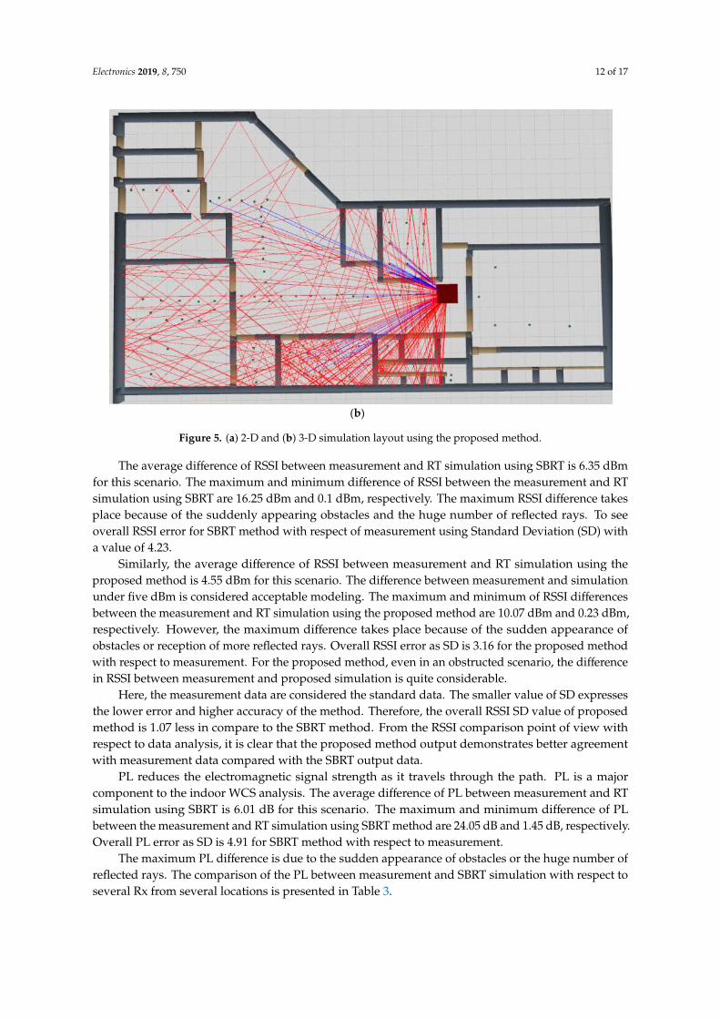
Figure 5. (a) 2-D and (b) 3-D simulation layout using the proposed method.

The average difference of RSSI between measurement and RT simulation using SBRT is 6.35 dBm

for this scenario. The maximum and minimum difference of RSSI between the measurement and RT

simulation using SBRT are 16.25 dBm and 0.1 dBm, respectively. The maximum RSSI difference takes

place because of the suddenly appearing obstacles and the huge number of reflected rays. To see

overall RSSI error for SBRT method with respect of measurement using Standard Deviation (SD) with

a value of 4.23.

Similarly, the average difference of RSSI between measurement and RT simulation using the

proposed method is 4.55 dBm for this scenario. The difference between measurement and simulation

under five dBm is considered acceptable modeling. The maximum and minimum of RSSI differences

between the measurement and RT simulation using the proposed method are 10.07 dBm and 0.23 dBm,

respectively. However, the maximum difference takes place because of the sudden appearance of

obstacles or reception of more reflected rays. Overall RSSI error as SD is 3.16 for the proposed method

with respect to measurement. For the proposed method, even in an obstructed scenario, the difference

in RSSI between measurement and proposed simulation is quite considerable.

Here, the measurement data are considered the standard data. The smaller value of SD expresses

the lower error and higher accuracy of the method. Therefore, the overall RSSI SD value of proposed

method is 1.07 less in compare to the SBRT method. From the RSSI comparison point of view with

respect to data analysis, it is clear that the proposed method output demonstrates better agreement

with measurement data compared with the SBRT output data.

PL reduces the electromagnetic signal strength as it travels through the path. PL is a major

component to the indoor WCS analysis. The average difference of PL between measurement and RT

simulation using SBRT is 6.01 dB for this scenario. The maximum and minimum difference of PL

between the measurement and RT simulation using SBRT method are 24.05 dB and 1.45 dB, respectively.

Overall PL error as SD is 4.91 for SBRT method with respect to measurement.

The maximum PL difference is due to the sudden appearance of obstacles or the huge number of

reflected rays. The comparison of the PL between measurement and SBRT simulation with respect to

several Rx from several locations is presented in Table 3.

Electronics 2019, 8, 750 13 of 17

Table 3. Comparison of path loss using measurement, SBRT, and the proposed method.

Mobile Station ID Measurement PL (dB) SBRT Method PL (dB) Proposed Method PL (dB)

Rx1 55.5 47.29 47.54Rx2 55.3 51.56 52.60Rx3 55.2 56.40 53.14Rx4 55.8 58.33 57.08Rx5 55.8 57.25 58.86Rx6 55.2 60.32 57.53Rx7 55.3 61.69 60.91Rx8 55.3 60.69 62.68Rx9 55.3 61.42 63.58Rx10 55.6 57.43 61.67Rx13 65.2 67.37 66.59Rx15 65.1 59.31 60.49Rx18 65.6 68.92 60.03Rx19 65.6 60.19 56.27Rx20 65.7 67.94 62.35Rx21 65.5 57.19 69.13Rx24 62.7 71.46 71.46Rx28 62.5 38.45 69.10Rx33 59.6 53.80 51.63Rx34 59.6 44.59 49.44Rx35 59.5 52.84 52.20Rx38 59.4 56.95 57.32Rx39 59.4 53.09 53.09

The average difference of PL between the measurement and RT simulation using the proposed

method is 5.38 dB for this scenario. The maximum and minimum difference of PL between the

measurement and RT proposed method simulation are 10.16 dB and 1.39 dB, respectively. Overall PL

error as SD is 2.69 for the proposed method with respect to measurement. However, the maximum PL

difference takes place because of the sudden appearance of obstacles or the huge number of reflected

rays. Moreover, for the proposed method, even in obstructed scenarios, the difference in PL between

measurement and the proposed method simulation is quite considerable. The comparison of the PL

between proposed RT simulation and measurement with respect to several Rx from different locations

is presented in Table 3.

Figure 6 shows the graphical view of PL comparison among three sets of outputs data. Here, the

measurement data are considered the standard data, which will help to validate the RT simulation.

Consider the PL similarity trend of SBRT method: mobile stations Rx3, Rx5, Rx10, Rx13, Rx20,

Rx38, Rx4, Rx18, and Rx2 demonstrate the moderate match with the measurement data, respectively.

The average difference of PL from the measurement data to SBRT method data for those points is

2.33 dB. On the other hand, in the SBRT method, mobile stations Rx8, Rx19, Rx15, Rx33, Rx9, Rx39,

Rx7, Rx35, Rx1, Rx21, Rx24, Rx34, and Rx28 demonstrate the distance relationship of PL respectively

from the measurement data because of reflections. The average difference of PL from the measurement

data to SBRT method data for those mobile stations is 8.38 dB. Even for some mobile stations, such as

Rx8 near to Tx, comparative PL difference is high because of the large number of interactions. Again,

according to the lower PL similarity trend of the proposed method, mobile stations Rx4, Rx13, Rx3,

Rx38, Rx6, Rx2, Rx5, Rx20, Rx21, and Rx15 respectively demonstrate the good relationship with the

measurement data. The average PL difference from the measurement data to proposed method data for

those mobile stations is 2.65 dB. On the other hand, in the proposed method, mobile stations Rx18, Rx7,

Rx10, Rx39, Rx28, Rx35, Rx8, Rx1, Rx33, Rx9, Rx24, Rx19, and Rx34 demonstrate distance relationship

consecutively of PL from the measurement data, because of reflections. The average difference of

PL from the measurement data to proposed method data for those mobile stations is 7.48 dB. Even

some mobile stations such as Rx7 is nearby Tx, but comparative PL difference is high because of some

large reflections.

Electronics 2019, 8, 750 14 of 17

–

0

10

20

30

40

50

60

70

80

Pa

th L

oss

(d

B)

Recievers

Measurement Path Loss (dB) SBRT Path Loss(dB) Proposed Method Path Loss (dB)

Figure 6. Path loss comparison graph between measurement and SBRT, proposed method simulation.

Here, if we consider the more similar simulation as bearing the average PL difference with

measurement data below 5 dB, 9 receivers are found in the SBRT method and 10 receivers are found in

the proposed method. One other hand, if we consider the less similar simulation bearing the average

PL difference with measurement data above 5 dB, 14 receivers are found in SBRT method, 13 receivers

are found in the proposed method. Finally, the overall PL SD value of the proposed method is 2.69

less in comparison to the SBRT method. It expresses greater accuracy of the proposed method over

the SBRT method. From the PL comparison points of view with respect to data analysis and Figure 6,

it is clear that in the proposed method, PL demonstrates more agreement with measurement data

compared with the SBRT method.

The best RL plays a dynamic role in ray RT [37–42]. RL is the initial step of RT method. Therefore,

the best use of the RL phase makes the proposed method more efficient, adaptive, and appropriate.

The number of ray launchings needed for the proposed method is much fewer than that in the SBRT

method. To get good coverage, using RL potential zone is the main key contribution of the proposed

method. Hence, based on the stable coverage, good PL, lower propagation time, good RSSI, and best

RL, the proposed method demonstrates a good contribution in WCS.

8. Conclusions

In this paper, a 3-D RT method for 4.5-GHz indoor radio propagation prediction has been proposed.

It is a smarter, more effective way to categorize radio wave propagation for indoor scenarios using

computerized simulation tools. Here, the RT used for the simulation purpose adopts two individual

algorithms, the SBRT and the proposed efficient method. In this simulation, similar features of the

layout, obstacle attenuation values, and antenna patterns are used as in the measurement. In general,

it is difficult to get all values of the measurement and simulation to match the requirements of RSSI

and PL. Moreover, the overall statistics of the measurement and simulation values with respect to

RSSI and PL are reasonably similar. The proposed method output demonstrates more similarity with

measurement than with conventional SBRT. The reduction of the PL SD from 4.91 dB for SBRT to

2.69 dB for the proposed method is significant contribution of proposed method. The comparison

results show that the proposed RT is more accurate with respect to RSSI and PL. The proposed method

achieves a noticeable gain in terms of computational efficiency by delivering more accurate RSSI and

PL with respect to the standard measurement data.

Electronics 2019, 8, 750 15 of 17

Author Contributions: Conceptualization, F.H. and T.K.G.; Simulation, F.H.; Software Development, F.H.; Raytracing validation, F.H. and T.K.G.; Formal Analysis, S.A.; Resources, T.A.R.; Measurement & Investigation,M.N.H., K.D., and F.H.; Writing—Original Draft Preparation, F.H.; Writing—Review & Editing W.L., C.P.T., andF.H.; Visualization, S.A. and F.H.; Supervision, T.K.G.; Project Administration, T.K.G.; Funding Acquisition, T.K.G.,A.A., A.M., T.C.P., C.P.L., and V.T.

Funding: The R&D work and manuscript publication fees are funded by Project name “Mobile IOT: LocationAware” with bearing number (MMUE/180025).

Acknowledgments: Special thanks to Multimedia University, Telecom Malaysia, Universiti Teknologi Malaysia,and ICT Division Bangladesh for providing the comprehensive financial assistance to this research. Also, thanks toFRGS funding body to support the project title “Indoor Internet of Things (IOT) Tracking Algorithm Developmentbased on Radio Signal Characterisation” (grant no. FRGS/1/2018/TK08/MMU/02/1) for financial support.

Conflicts of Interest: The authors declare no conflict of interest.

References

1. Ai, Y.; Cheffena, M.; Li, Q. Power delay profile analysis and modeling of industrial indoor channels.

In Proceedings of the 9th European Conference on Antennas and Propagation (EuCAP), Lisbon, Portugal,

13–17 April 2015; pp. 1–5.

2. Andersen, J.B.; Chee, K.L.; Jacob, M.; Pedersen, G.F.; Kurner, T. Reverberation and Absorption in an Aircraft

Cabin With the Impact of Passengers. IEEE Trans. Antennas Propag. 2012, 60, 2472–2480. [CrossRef]

3. Andersen, J.; Rappaport, T.; Yoshida, S. Propagation measurements and models for wireless communications

channels. IEEE Commun. Mag. 1995, 33, 42–49. [CrossRef]

4. Mathar, R.; Reyer, M.; Schmeink, M. A Cube Oriented Ray Launching Algorithm for 3D Urban Field Strength

Prediction. In Proceedings of the IEEE International Conference on Communications, Glasgow, UK, 24–28

June 2007; pp. 5034–5039.

5. Ji, Z.; Li, B.-H.; Wang, H.-X.; Chen, H.-Y.; Sarkar, T. Efficient ray-tracing methods for propagation prediction

for indoor wireless communications. IEEE Antennas Propag. Mag. 2001, 43, 41–49.

6. Yun, Z.; Iskander, M.; Zhang, Z. Complex-Wall Effect on Propagation Characteristics and MIMO Capacities

for an Indoor Wireless Communication Environment. IEEE Trans. Antennas Propag. 2004, 52, 914–922.

[CrossRef]

7. Suzuki, Y.; Omiya, M. Computer simulation for a site-specific modeling of indoor radio wave propagation.

In Proceedings of the IEEE Region 10 Conference (TENCON), Singapore, 22–25 November 2016; pp. 123–126.

[CrossRef]

8. Bhuvaneshwari, A.; Hemalatha, R.; Satyasavithri, T. Path loss prediction analysis by ray tracing approach

for NLOS indoor propagation. In Proceedings of the International Conference on Signal. Processing and

Communication Engineering Systems, Guntur, India, 2–3 January 2015; pp. 486–491.

9. Shirai, H.; Sato, R.; Otoi, K. Electromagnetic Wave Propagation Estimation by 3-D SBR Method. In Proceedings

of the International Conference on Electromagnetics in Advanced Applications, Torino, Italy, 17–21 September

2007; pp. 129–132.

10. Chao-han, T.; Dan, S.; Yuqi, S.; You-gang, G. The Application of an Improved SBR Algorithm in Outdoor

Environment. In Proceedings of the 7th Asia-Pacific Conference on Environmental Electromagnetics (CEEM),

Hangzhou, China, 4–7 November 2015.

11. Flores, S.J.; Mayorgas, L.F.; Jimenez, F.A. Reception Algorithms for Ray Launching Modeling of Indoor

Propagation. In Proceedings of the IEEE Radio and Wireless Conference, Colorado Springs, CO, USA,

9–12 August 1998.

12. Zakharov, P.N.; Dudov, R.A.; Mikhailov, E.V.; Korolev, A.F.; Sukhorukov, A.P. Finite integration technique

capabilities for indoor propagation prediction. Proceedings of Loughborough Antennas & Propagation

Conference, Loughborough, UK, 16–17 November 2009; pp. 369–372.

13. Huit, T.; Mohammed, A. Assessment of multipath propagation for a 2.4 GHz short-range wireless

communication system. In Proceedings of the IEEE 65th Vehicular Technology Conference, Dublin,

Ireland, 22–25 April 2007; pp. 544–548.

14. Lee, J.W.H.; Lai, A.K.Y. FDTD analysis of indoor radio propagation. IEEE Antennas Propag. Soc. Int. Symp.

1998, 3, 1664–1667.

Electronics 2019, 8, 750 16 of 17

15. Nagy, L. Indoor propagation modeling for short range devices. In Proceedings of the Second European

Antennas and Propagation, Edinburgh, UK, 11–16 November 2007; pp. 1–6.

16. Wang, Y.; Safavi-Naeini, S.; Chaudhuri, S.K. A hybrid technique based on combining ray tracing and FDTD

methods for site-specific modeling of indoor radio wave propagation. IEEE Trans. Antennas Propag. 2000, 48,

743–754. [CrossRef]

17. Plets, D.; Joseph, W.; Vanhecke, K.; Martens, L. Exposure Optimization in Indoor Wireless Networks by

Heuristic Network Planning. Prog. Electromagn. Res. 2013, 139, 445–478. [CrossRef]

18. Azpilicueta, L.; Rawat, M.; Rawat, K.; Ghannouchi, F.M.; Falcone, F. A Ray Launching-Neural Network

Approach for Radio Wave Propagation Analysis in Complex Indoor Environments. IEEE Trans. Antennas

Propag. 2014, 62, 2777–2786. [CrossRef]

19. Shi, D.; Tang, X.; Wang, C. The acceleration of the shooting and bouncing ray tracing method on GPUs. In

Proceedings of the XXXIInd General Assembly and Scientific Symposium of the International Union of Radio

Science (URSI GASS), Montreal, QC, Canada, 19–26 August 2017; pp. 1–3. [CrossRef]

20. Azpilicueta, L.; Rawat, M.; Rawat, K.; Ghannouchi, F.M.; Falcone, F. Convergence analysis in deterministic

3D ray launching radio channel estimation in complex environments. Appl. Comput. Electromagn. Soc. J.

2014, 29, 256–271.

21. Granda, F.L.; Azpilicueta, L.; Agilar, D.; Vargas, C. 3D ray launching simulation of urban vehicle to

infrastructure radio propagation links. Congr. Cienc. Tecnol. 2018, 13, 113–116. [CrossRef]

22. Lostanlen, B.; Kürner, T. Ray Tracing Modeling. In LTE Advanced and Next Generation Wireless Networks:

Channel Modeling and Propagatio; Wiley: Hoboken, NJ, USA, 2012; pp. 271–291.

23. Chen, S.-H.; Jeng, S.-K. An SBR/image approach for radio wave propagation in indoor environments with

metallic furniture. IEEE Trans. Antennas Propag. 1997, 45, 98–106. [CrossRef]

24. Durgin, G.; Patwari, N.; Rappaport, T.S. An advanced 3D ray launching method for wireless propagation

prediction. In Proceedings of the IEEE 47th Vehicular Technology Conference. Technology in Motion,

Phoenix, AZ, USA, 4–7 May 1997; Volume 2, pp. 785–789.

25. Lee, B.S.; Nix, A.R.; McGeehan, J.P. A spatio temporal ray launching propagation model for UMTS picoand

microcellular environments. In Proceedings of the IEEE VTS 53rd Vehicular Technology Conference, Rhodes,

Greece, 6–9 May 2001; Volume 1, pp. 367–371.

26. Lee, B.S.; Nix, A.R.; McGeehan, J.P. Indoor space time propagation modeling using a ray launching technique.

In Proceedings of the Eleventh International Conference on Antennas and Propagation, Manchester, UK,

17–20 April 2001; Volume 1, pp. 279–283.

27. Stavrou, S.; Saunders, S.R. Review of constitutive parameters of building materials. In Proceedings of the

Antennas and Propagation Twelfth International Conference, Exeter, UK, 31 March–3 April 2007.

28. ITU-R WP3K Propagation data and prediction methods for the planning of indoor radio communication

systems and radio local area networks in the frequency range 900 MHz to 100 GHz. Draft revision of

recommendation ITU-R P.1238. 1999. Available online: https://www.itu.int/rec/R-REC-P.1238 (accessed on

15 March 2019).

29. Seidel, S.Y.; Rappaport, T.S. Site-specific propagation prediction for wireless in-building personal

communication system design. IEEE Trans. Veh. Technol. 1994, 43, 879–891. [CrossRef]

30. Whitteker, J.H. Measurements of path loss at 910 MHz for proposed microcell urban mobile systems. IEEE

Trans. Veh. Technol. 1998, 37, 125–129. [CrossRef]

31. Mohtashami, V.; Shishegar, A.A. Effects of geometrical uncertainties on ray tracing results for site-specific

indoor propagation modeling. In Proceedings of the IEEE-APS Topical Conference on Antennas and

Propagation in Wireless Communications, Torino, Italy, 9–13 September 2013.

32. Remcom. Wireless InSite Reference Manual, ver. 2.7.1, Commercial SW User-Manual; Remcom Inc.: State College,

PA, USA, 2014; Available online: https://cdn.thomasnet.com/ccp/30280960/29435.pdf (accessed on 15 March

2019).

33. ITU-R. P.2040, Effects of Building Materials and Structures on Radio Wave Propagation above about 100 MHz;

Technical report; Electronic Publication: Geneva, Switzerland, 2015; Available online: https://www.itu.int/

dms_pubrec/itu-r/rec/p/R-REC-P.2040-1-201507-I!!PDF-E.pdf (accessed on 15 January 2019).

34. ITU-R. P.2040, Effects of Building Materials and Structures on Radio Wave propagation above about 100 MHz;

International Telecommunication Union Radio Communication Sector: Geneva, Switzerland, 2013; Available

online: https://www.itu.int/rec/R-REC-P.2040-0-201309-S/en (accessed on 15 January 2019).

Electronics 2019, 8, 750 17 of 17

35. Correia, L.M.; Frances, P.O. Estimation of materials characteristics from power measurements at 60

GHz. In Proceedings of the IEEE International Symposium on Personal, Indoor and Mobile Radio

Communications, Wireless Networks—Catching the Mobile Future, Hague, The Netherlands, 18–23

September 1994; pp. 510–513.

36. Lott, M.; Forkel, I. A multi-wall-and-floor model for indoor radio propagation. In Proceedings of the IEEE

VTS 53rd Vehicular Technology Conference, Rhodes, Greece, 6–9 May 2001; pp. 464–468.

37. Hossain, F.; Geok, T.K.; Rahman, T.A.; Hindia, M.N.; Dimyati, K.; Abdaziz, A. Indoor Millimeter-Wave

Propagation Prediction by Measurement and Ray Tracing Simulation at 38 GHz. Symmetry 2018, 10, 464.

[CrossRef]

38. Geok, T.K.; Hossain, F.; Kamaruddin, M.N.; Rahman, N.Z.A.; Thiagarajah, S.; Chiat, A.T.W.; Liew, C.P. A

Comprehensive Review of Efficient Ray-Tracing Techniques for Wireless Communication. Int. J. Commun.

Antenna Propag. 2018, 8, 123–136. [CrossRef]

39. Geok, T.K.; Hossain, F.; Chiat, A.T.W. A novel 3D ray launching technique for radio propagation prediction

in indoor environments. PLoS ONE 2018, 13. [CrossRef] [PubMed]

40. Hossain, F.; Geok, T.K.; Rahman, T.A.; Hindia, M.N.; Dimyati, K.; Tso, C.P.; Kamaruddin, M.N. Smart 3-D RT

Method: Indoor Radio Wave Propagation Modeling at 28 GHz. Symmetry 2018, 11, 510. [CrossRef]

41. Hong, Q.; Zhang, J.; Zheng, H.; Li, H.; Hu, H.; Zhang, B.; Lai, Z.; Zhang, J. The Impact of Antenna Height on

3D Channel: A Ray Launching Based Analysis. Electronics 2018, 7, 2. [CrossRef]

42. Hossain, F.; Geok, T.K.; Rahman, T.A.; Hindia, M.N.; Dimyati, K.; Ahmed, S.; Tso, C.P.; Abd Rahman, N.Z.

An Efficient 3-D Ray Tracing Method: Prediction of Indoor Radio Propagation at 28 GHz in 5G Network.

Electronics 2019, 8, 286. [CrossRef]

© 2019 by the authors. Licensee MDPI, Basel, Switzerland. This article is an open access

article distributed under the terms and conditions of the Creative Commons Attribution

(CC BY) license (http://creativecommons.org/licenses/by/4.0/).