Embed Size (px)
Citation preview

Under review as a conference paper at ICLR 2020
INDIVIDUALISED DOSE-RESPONSE ESTIMATIONUSING GENERATIVE ADVERSARIAL NETS
Anonymous authorsPaper under double-blind review
ABSTRACT
The problem of estimating treatment responses from observational data is bynow a well-studied one. Less well studied, though, is the problem of treatmentresponse estimation when the treatments are accompanied by a continuous dosageparameter. In this paper, we tackle this lesser studied problem by building on amodification of the generative adversarial networks (GANs) framework that hasalready demonstrated effectiveness in the former problem. Our model, DRGAN, isflexible, capable of handling multiple treatments each accompanied by a dosageparameter. The key idea is to use a significantly modified GAN model to generateentire dose-response curves for each sample in the training data which will thenallow us to use standard supervised methods to learn an inference model capableof estimating these curves for a new sample. Our model consists of 3 blocks: (1)a generator, (2) a discriminator, (3) an inference block. In order to address thechallenge presented by the introduction of dosages, we propose novel architecturesfor both our generator and discriminator. We model the generator as a multi-task deep neural network. In order to address the increased complexity of thetreatment space (because of the addition of dosages), we develop a hierarchicaldiscriminator consisting of several networks: (a) a treatment discriminator, (b) adosage discriminator for each treatment. In the experiments section, we introducea new semi-synthetic data simulation for use in the dose-response setting anddemonstrate improvements over the existing benchmark models.
1 INTRODUCTION
Most of the methods developed in the causal inference literature focus on learning the effects ofbinary or categorical treatments (Bertsimas et al., 2017; Alaa et al., 2017; Alaa & van der Schaar,2017; Athey & Imbens, 2016; Wager & Athey, 2018; Yoon et al., 2018). These treatments, though,are often administered at a certain dosage which can take on continuous values (such as vasopressors(Döpp-Zemel & Groeneveld, 2013)). In medicine, using a high dosage of a drug can lead to toxiceffects while using a low dosage can result in no effect on the patient outcome (Wang et al., 2017).Moreover, the dosage levels used when choosing between multiple treatments for a patient are crucialfor the decision (Rothwell et al., 2018).
While admissible dosage intervals for drugs are often determined from clinical trials (Cook et al.,2015), these trials often have a small number of patients and use simplistic mathematical models toassign dosage levels to patients that do not take into account patient heterogeneity (Ursino et al., 2017).After drugs are approved through clinical trials, observational data collected about different treatmentdosages prescribed to a diverse set of patients offers us the opportunity to learn individualizedresponses. As the relationships between treatment dosage efficacy, toxicity and patient featuresbecome more complex, estimating dose-response from observational data becomes particularlyimportant in order to identify optimal dosages for each patient. Fortunately, there is a wealth ofobservational data available in the medical domain from electronic health records (Henry et al., 2016).
Learning from observational data already presents significant challenges in the binary treatmentsetting. As explained by Spirtes (2009), in an observational treatment-effect dataset, only the factualoutcome is present (i.e. the outcome for the treatment that was actually given) - the counterfactualoutcomes are not observed. This problem is exacerbated in the dose-response setting in which thenumber of counterfactuals is no longer even finite. Moreover, the treatment assignment is non-random
1
Under review as a conference paper at ICLR 2020
Patie
nt o
utco
me
Dosage
DRGAN Counterfactual Generator
Dosage
DRGAN Discriminator
d<latexit sha1_base64="(null)">(null)</latexit><latexit sha1_base64="(null)">(null)</latexit><latexit sha1_base64="(null)">(null)</latexit><latexit sha1_base64="(null)">(null)</latexit> d
<latexit sha1_base64="(null)">(null)</latexit><latexit sha1_base64="(null)">(null)</latexit><latexit sha1_base64="(null)">(null)</latexit><latexit sha1_base64="(null)">(null)</latexit>
Treatment 1 Treatment 2
GANITE Counterfactual Generator
GANITE Discriminator
Patient outcome for treatment 1 Patient outcome
for treatment 2
Factual outcome
Backpropagation
Counterfactual outcomes
Patie
nt o
utco
me
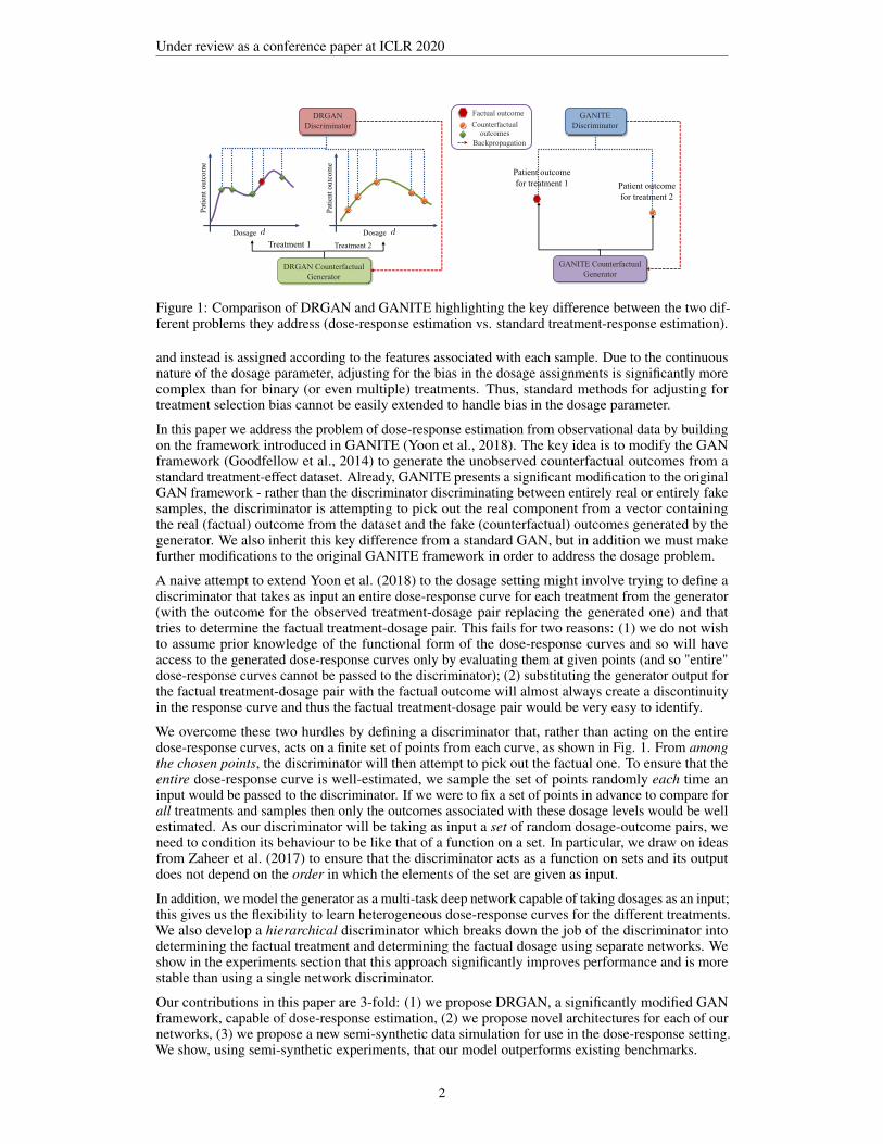
Figure 1: Comparison of DRGAN and GANITE highlighting the key difference between the two dif-ferent problems they address (dose-response estimation vs. standard treatment-response estimation).
and instead is assigned according to the features associated with each sample. Due to the continuousnature of the dosage parameter, adjusting for the bias in the dosage assignments is significantly morecomplex than for binary (or even multiple) treatments. Thus, standard methods for adjusting fortreatment selection bias cannot be easily extended to handle bias in the dosage parameter.
In this paper we address the problem of dose-response estimation from observational data by buildingon the framework introduced in GANITE (Yoon et al., 2018). The key idea is to modify the GANframework (Goodfellow et al., 2014) to generate the unobserved counterfactual outcomes from astandard treatment-effect dataset. Already, GANITE presents a significant modification to the originalGAN framework - rather than the discriminator discriminating between entirely real or entirely fakesamples, the discriminator is attempting to pick out the real component from a vector containingthe real (factual) outcome from the dataset and the fake (counterfactual) outcomes generated by thegenerator. We also inherit this key difference from a standard GAN, but in addition we must makefurther modifications to the original GANITE framework in order to address the dosage problem.
A naive attempt to extend Yoon et al. (2018) to the dosage setting might involve trying to define adiscriminator that takes as input an entire dose-response curve for each treatment from the generator(with the outcome for the observed treatment-dosage pair replacing the generated one) and thattries to determine the factual treatment-dosage pair. This fails for two reasons: (1) we do not wishto assume prior knowledge of the functional form of the dose-response curves and so will haveaccess to the generated dose-response curves only by evaluating them at given points (and so "entire"dose-response curves cannot be passed to the discriminator); (2) substituting the generator output forthe factual treatment-dosage pair with the factual outcome will almost always create a discontinuityin the response curve and thus the factual treatment-dosage pair would be very easy to identify.
We overcome these two hurdles by defining a discriminator that, rather than acting on the entiredose-response curves, acts on a finite set of points from each curve, as shown in Fig. 1. From amongthe chosen points, the discriminator will then attempt to pick out the factual one. To ensure that theentire dose-response curve is well-estimated, we sample the set of points randomly each time aninput would be passed to the discriminator. If we were to fix a set of points in advance to compare forall treatments and samples then only the outcomes associated with these dosage levels would be wellestimated. As our discriminator will be taking as input a set of random dosage-outcome pairs, weneed to condition its behaviour to be like that of a function on a set. In particular, we draw on ideasfrom Zaheer et al. (2017) to ensure that the discriminator acts as a function on sets and its outputdoes not depend on the order in which the elements of the set are given as input.
In addition, we model the generator as a multi-task deep network capable of taking dosages as an input;this gives us the flexibility to learn heterogeneous dose-response curves for the different treatments.We also develop a hierarchical discriminator which breaks down the job of the discriminator intodetermining the factual treatment and determining the factual dosage using separate networks. Weshow in the experiments section that this approach significantly improves performance and is morestable than using a single network discriminator.
Our contributions in this paper are 3-fold: (1) we propose DRGAN, a significantly modified GANframework, capable of dose-response estimation, (2) we propose novel architectures for each of ournetworks, (3) we propose a new semi-synthetic data simulation for use in the dose-response setting.We show, using semi-synthetic experiments, that our model outperforms existing benchmarks.
2

Under review as a conference paper at ICLR 2020
2 RELATED WORK
Methods for estimating the outcomes of treatments with an exposure dosage parameter that onlyemploy observational data make use of the generalized propensity score (GPS) (Imbens, 2000; Imai &Van Dyk, 2004; Hirano & Imbens, 2004) or build on top of balancing methods for multiple treatments.Schwab et al. (2019) developed a neural network based method to estimate counterfactuals formultiple treatments and continuous dosages. The proposed Dose Response networks (DRNets)in Schwab et al. (2019) consist of a three level architecture with shared layers for all treatments,multi-task layers for each treatment and additional multi-task layers for dosage sub-intervals. Morespecifically, for each treatment w, the dosage interval [aw, bw] is subdivided into E equally sizedsub-intervals and a multi-task head is added for each sub-interval. Their model architecture extendsthe one in Shalit et al. (2017) by adding the multi-task heads for the dosage strata. However, the mainadvantage of using multi-task heads for dosage intervals would be the added flexibility in the modelto learn potentially very different functions over different regions of the dosage interval. DRNetsdoes not determine the dosage intervals dynamically and thus much of this flexbility is lost. Wedemonstrate in our experiments that DRGAN outperforms both GPS and DRNets.
For a discussion of works that address treatment-response estimation without a dosage parameter, seeAppendix A. Note that for such methods we cannot treat the dosage as an additional input due to thebias associated with its assignment.
3 PROBLEM FORMULATION
We consider receiving observations of the form (xi, tif , yif ) for i = 1, ..., N , where, for each i, these
are independent realizations of the random variables (X, Tf , Yf ). We refer to X as the feature vectorlying in some feature space X , containing pre-treatment covariates (such as age, weight and labtest results). The treatment random variable, Tf , is in fact a pair of values Tf = (Wf , Df ) whereWf ∈ W corresponds to the type of treatment being administered (e.g. chemotherapy or radiotherapy)which lies in the discrete space of k treatments,W = {w1, ..., wk}, andDf corresponds to the dosageof the treatment (e.g. number of cycles, amount of chemotherapy, intensity of radiotherapy), which,for a given treatment w lies in the corresponding treatment’s dosage space, Dw, which in the mostgeneral case is some continuous space (e.g. the interval [0, 1]). We define the set of all treatment-dosage pairs to be T = {(w, d) : w ∈ W, d ∈ Dw}.Following Rubin’s potential outcome framework (Rubin, 1984), we assume that for all treatment-dosage pairs, (w, d), there is a potential outcome Y (w, d) ∈ Y (e.g. 1-year survival probability). Theobserved outcome is then defined to be Yf = Y (Wf , Df ). We will refer to the unobserved (potential)outcomes as counterfactuals.
The goal of dose-response estimation is to derive unbiased estimates of the potential outcomes for agiven set of input covariates:
µ(t,x) = E[Y (t)|X = x] (1)
for each t ∈ T , x ∈ X . We refer to µ(·) as the individualised dose-response function. In general, thisquantity is not the same as E[Y |X = x, Tf = t] (which can be easily estimated from observationaldata) in the presence of selection bias which often presents itself in observational datasets. In orderfor these two quantities to be equal, we must make the following common assumption.
Assumption 1. (Unconfoundedness) The treatment assignment, Tf , and potential outcomes, Y (w, d),are conditionally independent given the covariates X, i.e.
{Y (w, d)|w ∈ W, d ∈ Dw} ⊥⊥ Tf |X . (2)
This assumption is also commonly referred to as no hidden confounding.
In addition, in order to make µ(·) identifiable we must also assume that any treatment-dosage paircould be assigned to any given sample.
Assumption 2. (Overlap) For each x ∈ X such that p(x) > 0, we have 1 > p(t|x) > 0 for eacht ∈ T .
3

Under review as a conference paper at ICLR 2020
4 DOSE-RESPONSE GAN
We propose estimating µ by first training a generator to generate dose-response curves for each samplewithin the training dataset. The learned generator can then be used to train an inference network usingstandard supervised methods. We build on the idea presented in Yoon et al. (2018), using a modifiedGAN framework to generate potential outcomes conditional on the observed features, treatment andfactual outcome. Several changes must be made to both the generator and discriminator architecturesand learning paradigms in order to produce a model capable of handling the dose-response setting.
4.1 COUNTERFACTUAL GENERATOR
Our generator, G : X ×T ×Y ×Z → YT takes features, x ∈ X , factual outcome, yf ∈ Y , receivedtreatment and dosage, tf = (wf , df ) ∈ T , and some noise, z ∈ Z (typically multivariate uniform orGaussian), as inputs. The output will be a dose-response curve for each treatment (as shown in Fig.1), so that the output is a function from T to Y , i.e. G(x, tf , yf , z)(·) : T → Y . We can then write
ycf (t) = G(x, tf , yf , z)(t) (3)
to denote our generated counterfactual outcome for the treatment-dosage pair t. We will writeYcf (t) = G(X, Tf , Yf ,Z)(t) (i.e. the random variable induced by G).
While the job of the counterfactual generator is to generate outcomes for the treatment-dosage pairswhich were not observed, Yoon et al. (2018) demonstrated that the performance of the counterfactualgenerator is improved by adding a supervised loss term that regularises its output for the factualtreatment (in our case treatment-dosage pair). We define the supervised loss, LS , to be
LS(G) = E[(Yf −G(X, Tf , Yf ,Z)(Tf ))2
], (4)
where the expectation is taken over X, Tf , Yf and Z.
4.2 COUNTERFACTUAL DISCRIMINATOR
As noted in Section 1, our discriminator will act on a random set of points from each of the generateddose-response curves. Similar to Yoon et al. (2018), we define a discriminator, D, that will attempt topick out the factual treatment-dosage pair from among the (random set of) generated ones.
Formally, let nw ∈ Z+ be the number of dosage levels we will compare for treatment w ∈ W1.For each w ∈ W , let Dw = {Dw
1 , ..., Dwnw} be a random subset2 of Dw of size nw, where for
the factual treatment, Wf , DWfcontains nWf
− 1 random elements along with Df . We defineYw = (Dw
i , Ywi )nw
i=1 ∈ (Dw×Y)nw to be the vector of dosage-outcome pairs for treatment w where
Y wi =
{Yf if Wf = w and Df = Dw
i
Ycf (w,Dwi ) else
(5)
and will write Y = (Yw)w∈W . We will write dwj , yw and y to denote realisations of Dwj , Yw and y.
Our discriminator, D : X × ∏w∈W(Dw × Y)nw → [0, 1]∑nw , will take the features x ∈ X
together with the (random) set of generated outcomes y ∈ Y∑nw , and output a probability for each
treatment-dosage pair indicating the discriminator’s belief that that pair is the factual one.
As in the standard GAN framework, we define a minimax game by defining the value function to be
L(D,G) = E
[ ∑w∈W
∑d∈Dw
I{Tf=(w,d)} logDw,d(X, Y)+I{Tf 6=(w,d)} log(1−Dw,d(X, Y))
], (6)
where the expectation is taken over X, Tf , Y and {Dw : w ∈ W}, Dw,d corresponds to thediscriminator output for treatment-dosage pair (w, d).
1In practice we set all nw to be the same. The default setting is 5 in the experiments.2In practice, when Dw = [0, 1], each Dw
j is sampled independently and uniformly from [0, 1]. Note that foreach training iteration, Dw is resampled (see Section 1).
4

Under review as a conference paper at ICLR 2020
G<latexit sha1_base64="(null)">(null)</latexit><latexit sha1_base64="(null)">(null)</latexit><latexit sha1_base64="(null)">(null)</latexit><latexit sha1_base64="(null)">(null)</latexit>
Counterfactual generatorx
<latexit sha1_base64="(null)">(null)</latexit><latexit sha1_base64="(null)">(null)</latexit><latexit sha1_base64="(null)">(null)</latexit><latexit sha1_base64="(null)">(null)</latexit>
wf<latexit sha1_base64="(null)">(null)</latexit><latexit sha1_base64="(null)">(null)</latexit><latexit sha1_base64="(null)">(null)</latexit><latexit sha1_base64="(null)">(null)</latexit>
df<latexit sha1_base64="(null)">(null)</latexit><latexit sha1_base64="(null)">(null)</latexit><latexit sha1_base64="(null)">(null)</latexit><latexit sha1_base64="(null)">(null)</latexit>
y(w, d)<latexit sha1_base64="(null)">(null)</latexit><latexit sha1_base64="(null)">(null)</latexit><latexit sha1_base64="(null)">(null)</latexit><latexit sha1_base64="(null)">(null)</latexit>
yf<latexit sha1_base64="(null)">(null)</latexit><latexit sha1_base64="(null)">(null)</latexit><latexit sha1_base64="(null)">(null)</latexit><latexit sha1_base64="(null)">(null)</latexit>
z<latexit sha1_base64="(null)">(null)</latexit><latexit sha1_base64="(null)">(null)</latexit><latexit sha1_base64="(null)">(null)</latexit><latexit sha1_base64="(null)">(null)</latexit>
w<latexit sha1_base64="(null)">(null)</latexit><latexit sha1_base64="(null)">(null)</latexit><latexit sha1_base64="(null)">(null)</latexit><latexit sha1_base64="(null)">(null)</latexit> d
<latexit sha1_base64="(null)">(null)</latexit><latexit sha1_base64="(null)">(null)</latexit><latexit sha1_base64="(null)">(null)</latexit><latexit sha1_base64="(null)">(null)</latexit>
y(wf , df )<latexit sha1_base64="(null)">(null)</latexit><latexit sha1_base64="(null)">(null)</latexit><latexit sha1_base64="(null)">(null)</latexit><latexit sha1_base64="(null)">(null)</latexit>
LW<latexit sha1_base64="(null)">(null)</latexit><latexit sha1_base64="(null)">(null)</latexit><latexit sha1_base64="(null)">(null)</latexit><latexit sha1_base64="(null)">(null)</latexit>
Ld<latexit sha1_base64="(null)">(null)</latexit><latexit sha1_base64="(null)">(null)</latexit><latexit sha1_base64="(null)">(null)</latexit><latexit sha1_base64="(null)">(null)</latexit>
DW<latexit sha1_base64="(null)">(null)</latexit><latexit sha1_base64="(null)">(null)</latexit><latexit sha1_base64="(null)">(null)</latexit><latexit sha1_base64="(null)">(null)</latexit>
Dwcf<latexit sha1_base64="(null)">(null)</latexit><latexit sha1_base64="(null)">(null)</latexit><latexit sha1_base64="(null)">(null)</latexit><latexit sha1_base64="(null)">(null)</latexit>
Dwf<latexit sha1_base64="(null)">(null)</latexit><latexit sha1_base64="(null)">(null)</latexit><latexit sha1_base64="(null)">(null)</latexit><latexit sha1_base64="(null)">(null)</latexit>
DH<latexit sha1_base64="(null)">(null)</latexit><latexit sha1_base64="(null)">(null)</latexit><latexit sha1_base64="(null)">(null)</latexit><latexit sha1_base64="(null)">(null)</latexit>
y<latexit sha1_base64="(null)">(null)</latexit><latexit sha1_base64="(null)">(null)</latexit><latexit sha1_base64="(null)">(null)</latexit><latexit sha1_base64="(null)">(null)</latexit>
x<latexit sha1_base64="(null)">(null)</latexit><latexit sha1_base64="(null)">(null)</latexit><latexit sha1_base64="(null)">(null)</latexit><latexit sha1_base64="(null)">(null)</latexit>
ywcf<latexit sha1_base64="(null)">(null)</latexit><latexit sha1_base64="(null)">(null)</latexit><latexit sha1_base64="(null)">(null)</latexit><latexit sha1_base64="(null)">(null)</latexit>
ywf<latexit sha1_base64="(null)">(null)</latexit><latexit sha1_base64="(null)">(null)</latexit><latexit sha1_base64="(null)">(null)</latexit><latexit sha1_base64="(null)">(null)</latexit>
Dwf<latexit sha1_base64="(null)">(null)</latexit><latexit sha1_base64="(null)">(null)</latexit><latexit sha1_base64="(null)">(null)</latexit><latexit sha1_base64="(null)">(null)</latexit>
Dwcf<latexit sha1_base64="(null)">(null)</latexit><latexit sha1_base64="(null)">(null)</latexit><latexit sha1_base64="(null)">(null)</latexit><latexit sha1_base64="(null)">(null)</latexit>
LS<latexit sha1_base64="(null)">(null)</latexit><latexit sha1_base64="(null)">(null)</latexit><latexit sha1_base64="(null)">(null)</latexit><latexit sha1_base64="(null)">(null)</latexit>
LG<latexit sha1_base64="(null)">(null)</latexit><latexit sha1_base64="(null)">(null)</latexit><latexit sha1_base64="(null)">(null)</latexit><latexit sha1_base64="(null)">(null)</latexit>
ywf<latexit sha1_base64="(null)">(null)</latexit><latexit sha1_base64="(null)">(null)</latexit><latexit sha1_base64="(null)">(null)</latexit><latexit sha1_base64="(null)">(null)</latexit>
ywcf<latexit sha1_base64="(null)">(null)</latexit><latexit sha1_base64="(null)">(null)</latexit><latexit sha1_base64="(null)">(null)</latexit><latexit sha1_base64="(null)">(null)</latexit>
x<latexit sha1_base64="(null)">(null)</latexit><latexit sha1_base64="(null)">(null)</latexit><latexit sha1_base64="(null)">(null)</latexit><latexit sha1_base64="(null)">(null)</latexit>
wf<latexit sha1_base64="(null)">(null)</latexit><latexit sha1_base64="(null)">(null)</latexit><latexit sha1_base64="(null)">(null)</latexit><latexit sha1_base64="(null)">(null)</latexit>
df<latexit sha1_base64="(null)">(null)</latexit><latexit sha1_base64="(null)">(null)</latexit><latexit sha1_base64="(null)">(null)</latexit><latexit sha1_base64="(null)">(null)</latexit>
yf<latexit sha1_base64="(null)">(null)</latexit><latexit sha1_base64="(null)">(null)</latexit><latexit sha1_base64="(null)">(null)</latexit><latexit sha1_base64="(null)">(null)</latexit>
z<latexit sha1_base64="(null)">(null)</latexit><latexit sha1_base64="(null)">(null)</latexit><latexit sha1_base64="(null)">(null)</latexit><latexit sha1_base64="(null)">(null)</latexit>
w<latexit sha1_base64="(null)">(null)</latexit><latexit sha1_base64="(null)">(null)</latexit><latexit sha1_base64="(null)">(null)</latexit><latexit sha1_base64="(null)">(null)</latexit>
d<latexit sha1_base64="(null)">(null)</latexit><latexit sha1_base64="(null)">(null)</latexit><latexit sha1_base64="(null)">(null)</latexit><latexit sha1_base64="(null)">(null)</latexit>
Features
Factual treatment
Factual dosage
Factual outcome
Noise vector
Treatment to generate
Dosage to generate
Dwcf<latexit sha1_base64="(null)">(null)</latexit><latexit sha1_base64="(null)">(null)</latexit><latexit sha1_base64="(null)">(null)</latexit><latexit sha1_base64="(null)">(null)</latexit>
Random dosage samples for treatment
ywcf<latexit sha1_base64="(null)">(null)</latexit><latexit sha1_base64="(null)">(null)</latexit><latexit sha1_base64="(null)">(null)</latexit><latexit sha1_base64="(null)">(null)</latexit>
Generated dosage-outcome pairs for treatment
y<latexit sha1_base64="(null)">(null)</latexit><latexit sha1_base64="(null)">(null)</latexit><latexit sha1_base64="(null)">(null)</latexit><latexit sha1_base64="(null)">(null)</latexit>
Generated dosage-outcome pairs for all treatmentsInput/outputBackpropagation
⇥<latexit sha1_base64="(null)">(null)</latexit><latexit sha1_base64="(null)">(null)</latexit><latexit sha1_base64="(null)">(null)</latexit><latexit sha1_base64="(null)">(null)</latexit>
+<latexit sha1_base64="(null)">(null)</latexit><latexit sha1_base64="(null)">(null)</latexit><latexit sha1_base64="(null)">(null)</latexit><latexit sha1_base64="(null)">(null)</latexit>
w<latexit sha1_base64="(null)">(null)</latexit><latexit sha1_base64="(null)">(null)</latexit><latexit sha1_base64="(null)">(null)</latexit><latexit sha1_base64="(null)">(null)</latexit>
w<latexit sha1_base64="(null)">(null)</latexit><latexit sha1_base64="(null)">(null)</latexit><latexit sha1_base64="(null)">(null)</latexit><latexit sha1_base64="(null)">(null)</latexit>
Figure 2: Overview of our model for the setting with two treatments (wf corresponds to the factualtreatment and wcf to the counterfactual treatment). The generator is used to generate an output foreach dosage level in each Dw, these outcomes together with the factual outcome, yf , are used tocreate the set of dosage-outcome pairs, y, which is passed directly to the treatment discriminator.Each dosage discriminator receives only the part of y corresponding to that treatment, i.e. yw. Thesediscriminators are combined (Eq. 11) to define DH which is used to give feedback to the generator.
The minimax game is then given byminG
maxDL(D,G) + λLS(G) , (7)
where λ is used to control the trade-off between L and LS (we set λ = 1 in the experiments).
The task of the discriminator (i.e. picking out the factual dosage from∑kj=1 nwj treatment-dosage
pairs) becomes increasingly difficult as we increase nw or k because the dimension of the discrimi-nator output space,
∑nw, increases. Although we control nw, if we set it too low, then the set yw
may not well-represent the dose-response curve, particularly if the dose-response curve is complex.In practice we found that even for moderate settings of nw and only 2 treatments, modelling thediscriminator as a single function resulted in poor performance. In order to overcome this problem,we introduce a novel hierarchical discriminator which involves a treatment discriminator with outputdimension k and several dosage discriminators, one for each treatment, with output dimensions nw.
First observe that the probability P((Wf , Df ) = (w, d)|X, Dw, Y) can be written as
P(Wf = w|X, Dw, Y)× P(Df = d|Wf = w,X, Dw, Y) . (8)We can therefore break down the discriminator into a hierarchical model by learning one discriminator,DW , that outputs P(Wf = w|X, Dw, Y) which we will refer to as the treatment discriminator, andthen a discriminator, Dw, for each treatment, w ∈ W , that outputs P(Df = d|Wf = w,X, Dw, Y)which we will refer to as the dosage discriminator for treatment w.
The treatment discriminator, DW : X×∏w∈W(Dw × Y)nw → [0, 1]k, takes the features, x, andgenerated potential outcomes, y, and outputs a probability for each treatment, w1, ..., wk. WritingDwW to denote the output of DW corresponding to treatment w, we define the loss, LW , to be
LW(DW ;G) = −E[ ∑w∈W
I{Wf=w} logDwW(X, Y) + I{Wf 6=w} log(1−Dw
W(X, Y))
], (9)
where, again, the expectation is taken over X,Wf , Df , Y and {Dw}w∈W .
Then, for each w ∈ W , Dw : X × (Dw × Y)nw → [0, 1]nw is a map that takes the features, x, andgenerated potential outcomes, yw, corresponding to treatment w and outputs a probability for eachdosage level, dw1 , ..., d
wnw
, in a given realisation of Dw. Writing Djw to denote the output of Dw
corresponding to dosage level Dwj , we define the loss of each dosage discriminator to be
Ld(Dw;G) = −E[I{Wf=w}
nw∑j=1
I{Df=Dwj } logDj
w(X, Yw)+I{Df 6=Dwj } log(1−Dj
w(X, Yw))
],
(10)
5

Under review as a conference paper at ICLR 2020
where the expectation is taken over X, Dw, Yw,Wf and Df . The I{Wf=w} term ensures that onlysamples for which the factual treatment is w are used to train dosage discriminator Dw (otherwisethere would be no factual dosage for that sample).
We define the overall discriminator DH : X ×∏w∈W(Dw × Y )nw → [0, 1]∑nw by defining its
output corresponding to the treatment-dosage pair (w, dwj ) as
Dw,jH (x, y) = Dw
W(x, y)×Djw(x, yw) . (11)
Instead of the minimax game in Eq. 7, the generator and discriminator are trained according to theminimax game defined by seeking G∗, D∗H that solve
G∗ = arg minGL(D∗H ;G) + λLS(G) D∗H
w,j = D∗Ww ×D∗w
j
D∗W = arg minDWLW(DW ;G∗) D∗w = arg min
Dw
Ld(Dw;G∗),∀w ∈ W (12)
Fig. 2 depicts our generator and hierarchical discriminator. Pseudo-code for our algorithm can befound in Appendix C.
4.3 INFERENCE NETWORK
Once we have learned the counterfactual generator, we can use it only to access (generated) dose-response curves for all samples in the dataset. To generate dose-response curves for a new samplewe use the counterfactual generator along with the original data to train an inference network,I : X × T → Y . Details of the loss and pseudo-code can be found in Appendix D.
5 ARCHITECTURE
In this section, we describe in detail the novel architectures that we adopt to model each of thefunctions G,D,DW ,Dw1 , ...,Dwk
which draws from the ideas in Zaheer et al. (2017). The inferencenetwork, I, has the same architecture as the generator, but does not receive wf , df , yf or z as inputs.
5.1 GENERATOR ARCHITECTURE
Shared layer
wf<latexit sha1_base64="(null)">(null)</latexit><latexit sha1_base64="(null)">(null)</latexit><latexit sha1_base64="(null)">(null)</latexit><latexit sha1_base64="(null)">(null)</latexit>
df<latexit sha1_base64="(null)">(null)</latexit><latexit sha1_base64="(null)">(null)</latexit><latexit sha1_base64="(null)">(null)</latexit><latexit sha1_base64="(null)">(null)</latexit>
yf<latexit sha1_base64="(null)">(null)</latexit><latexit sha1_base64="(null)">(null)</latexit><latexit sha1_base64="(null)">(null)</latexit><latexit sha1_base64="(null)">(null)</latexit>
z<latexit sha1_base64="(null)">(null)</latexit><latexit sha1_base64="(null)">(null)</latexit><latexit sha1_base64="(null)">(null)</latexit><latexit sha1_base64="(null)">(null)</latexit>
d<latexit sha1_base64="(null)">(null)</latexit><latexit sha1_base64="(null)">(null)</latexit><latexit sha1_base64="(null)">(null)</latexit><latexit sha1_base64="(null)">(null)</latexit>
x<latexit sha1_base64="(null)">(null)</latexit><latexit sha1_base64="(null)">(null)</latexit><latexit sha1_base64="(null)">(null)</latexit><latexit sha1_base64="(null)">(null)</latexit>
y(w, d)<latexit sha1_base64="(null)">(null)</latexit><latexit sha1_base64="(null)">(null)</latexit><latexit sha1_base64="(null)">(null)</latexit><latexit sha1_base64="(null)">(null)</latexit>
w<latexit sha1_base64="(null)">(null)</latexit><latexit sha1_base64="(null)">(null)</latexit><latexit sha1_base64="(null)">(null)</latexit><latexit sha1_base64="(null)">(null)</latexit>
Figure 3: Generator architecture.
We adopt a multi-task deep learning model for G by defininga function g : X × T × Y × Z → H for some latent space H(typically Rl for some l) and then for each treatment w ∈ W weintroduce a multitask "head", gw : H×Dw → Y taking inputsfrom H and a dosage, d, to produce an outcome y(w, d) ∈ Y .Given observations, (x, tf , yf ), a noise vector z, and a targettreatment-dosage pair, t = (w, d), we define
G(x, tf , yf , z)(t) = gw(g(x, tf , yf , z), d) . (13)
Each of g, gw1, ..., gwk
are modelled as fully connected networks.Fig. 3 depicts our generator architecture.
5.2 DISCRIMINATOR ARCHITECTURES
As noted in Section 1, our discriminators need to act as functions of sets (of randomly selected dosage-outcome pairs). While we could require that our discriminators try to learn this during training, byenforcing them to be functions of sets through their architecture, we reduce the complexity of learningthe discriminators (they no longer need to "rule out" functions which are not functions of sets). Thisresults in better performing discriminators, which in turn improves the performance of the generator.
In practice, the treatment discriminator receives all of the sets (i.e. one set for each treatment)of dosage-outcome pairs and outputs a probability for each treatment (i.e. there is one outputcorresponding to each set). In order to define such a function, we treat each input set as a vector butrequire that the outputs be invariant to (i.e. should not depend on) the ordering of the set as a vector.
6
Under review as a conference paper at ICLR 2020
Each dosage discriminator receives the set corresponding to a given treatment and is tasked withoutputting a probability for each element in the set. In order to define such a function, we considerthe input and output as vectors but then require that if we permute the elements of the input vector,the output should be permuted in the same way. We formalise the required notions - permutationinvariance and permutation equivariance (Zaheer et al., 2017) - in the following subsection.
5.2.1 PERMUTATION INVARIANCE AND PERMUTATION EQUIVARIANCE
The notions of what it means for a function to be permutation invariant and permutation equivariantwith respect to (a subset of) its inputs are given below in definitions 1 and 2, respectively. Let U , V , Cbe some spaces. Let m ∈ Z+.Definition 1. A function f : Um × V → C is permutation invariant with respect to the space Um iffor every u = (u1, ..., um) ∈ Um, every v ∈ V and every permutation, σ, of {1, ...,m} we have
f(u1, ..., um, v) = f(uσ(1), ..., uσ(m), v) . (14)
Definition 2. A function f : Um×V → Cm is permutation equivariant with respect to the space Umif for every u = (u1, ..., um) ∈ Um, every v ∈ V and every permutation, σ, of {1, ...,m} we have
f(uσ(1), ..., uσ(m), v) = (fσ(1)(u, v), ..., fσ(m)(u, v)) , (15)
where fj(u, v) is the jth element of f(u, v).
To build up functions that are permutation invariant and permutation equivariant we make thefollowing observations: (1) the composition of any function with a permutation invariant function ispermutation invariant, (2) the composition of two permutation equivariant functions is permutationequivariant.
Zaheer et al. (2017) provide several possible building blocks to use to construct invariant andequivariant deep networks. The basic building block we will use for invariant functions will be alayer of the form
finv(u) = σ(1b1Tm(φ(u1), ..., φ(um))) , (16)
where 1l is a vector of 1s of dimension l, φ is any function φ : U → Rq for some q (in this paper weuse a standard fully connected layer) and σ is some non-linearity.
The basic building block for equivariant functions is defined in terms of an equivariance input, u, andan auxiliary input, v, by
fequi(u,v) = σ(λImu + γ(1m1Tm)u + (1mΘT )v) , (17)
where Im is the m×m identity matrix, λ and γ are scalar parameters and Θ is a vector of weights.
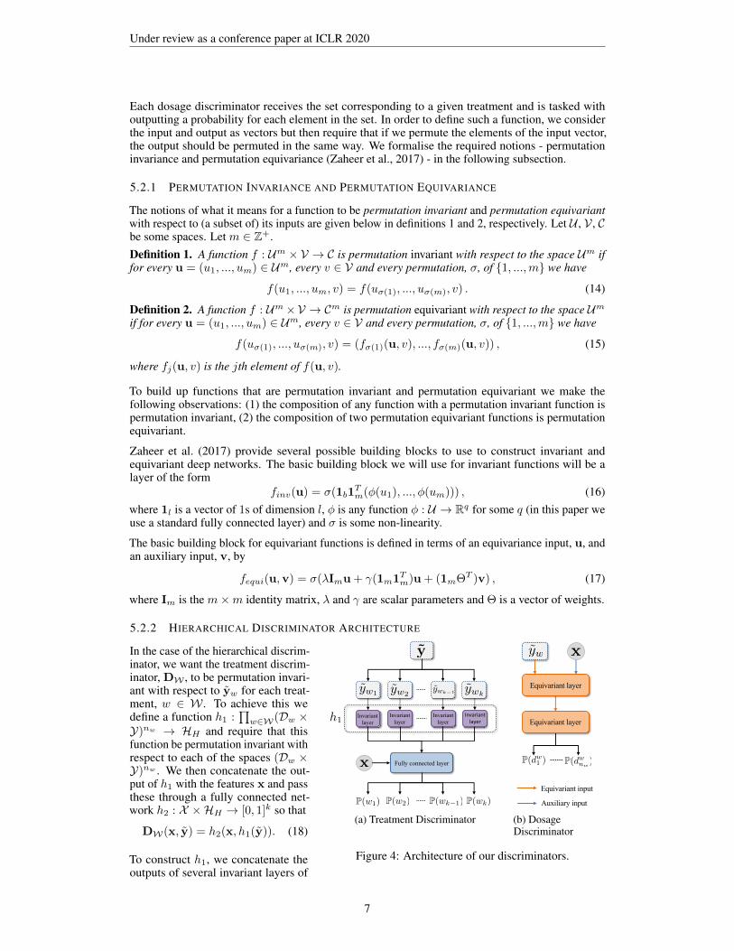
5.2.2 HIERARCHICAL DISCRIMINATOR ARCHITECTURE
y<latexit sha1_base64="(null)">(null)</latexit><latexit sha1_base64="(null)">(null)</latexit><latexit sha1_base64="(null)">(null)</latexit><latexit sha1_base64="(null)">(null)</latexit>
x<latexit sha1_base64="(null)">(null)</latexit><latexit sha1_base64="(null)">(null)</latexit><latexit sha1_base64="(null)">(null)</latexit><latexit sha1_base64="(null)">(null)</latexit>
x<latexit sha1_base64="(null)">(null)</latexit><latexit sha1_base64="(null)">(null)</latexit><latexit sha1_base64="(null)">(null)</latexit><latexit sha1_base64="(null)">(null)</latexit>
Equivariant layer
Equivariant layer
Equivariant input
Auxiliary input
Fully connected layer
Invariant layer
Invariant layer
Invariant layer
Invariant layer
yw1<latexit sha1_base64="(null)">(null)</latexit><latexit sha1_base64="(null)">(null)</latexit><latexit sha1_base64="(null)">(null)</latexit><latexit sha1_base64="(null)">(null)</latexit>
yw2<latexit sha1_base64="(null)">(null)</latexit><latexit sha1_base64="(null)">(null)</latexit><latexit sha1_base64="(null)">(null)</latexit><latexit sha1_base64="(null)">(null)</latexit>
ywk�1<latexit sha1_base64="(null)">(null)</latexit><latexit sha1_base64="(null)">(null)</latexit><latexit sha1_base64="(null)">(null)</latexit><latexit sha1_base64="(null)">(null)</latexit>
ywk<latexit sha1_base64="(null)">(null)</latexit><latexit sha1_base64="(null)">(null)</latexit><latexit sha1_base64="(null)">(null)</latexit><latexit sha1_base64="(null)">(null)</latexit>
P(w1)<latexit sha1_base64="(null)">(null)</latexit><latexit sha1_base64="(null)">(null)</latexit><latexit sha1_base64="(null)">(null)</latexit><latexit sha1_base64="(null)">(null)</latexit>
P(w2)<latexit sha1_base64="(null)">(null)</latexit><latexit sha1_base64="(null)">(null)</latexit><latexit sha1_base64="(null)">(null)</latexit><latexit sha1_base64="(null)">(null)</latexit>
P(wk�1)<latexit sha1_base64="(null)">(null)</latexit><latexit sha1_base64="(null)">(null)</latexit><latexit sha1_base64="(null)">(null)</latexit><latexit sha1_base64="(null)">(null)</latexit>
P(wk)<latexit sha1_base64="(null)">(null)</latexit><latexit sha1_base64="(null)">(null)</latexit><latexit sha1_base64="(null)">(null)</latexit><latexit sha1_base64="(null)">(null)</latexit>
yw<latexit sha1_base64="(null)">(null)</latexit><latexit sha1_base64="(null)">(null)</latexit><latexit sha1_base64="(null)">(null)</latexit><latexit sha1_base64="(null)">(null)</latexit>
P(dwnw
)<latexit sha1_base64="(null)">(null)</latexit><latexit sha1_base64="(null)">(null)</latexit><latexit sha1_base64="(null)">(null)</latexit><latexit sha1_base64="(null)">(null)</latexit>
P(dw1 )
<latexit sha1_base64="(null)">(null)</latexit><latexit sha1_base64="(null)">(null)</latexit><latexit sha1_base64="(null)">(null)</latexit><latexit sha1_base64="(null)">(null)</latexit>
h1<latexit sha1_base64="(null)">(null)</latexit><latexit sha1_base64="(null)">(null)</latexit><latexit sha1_base64="(null)">(null)</latexit><latexit sha1_base64="(null)">(null)</latexit>
(a) Treatment Discriminator
y<latexit sha1_base64="(null)">(null)</latexit><latexit sha1_base64="(null)">(null)</latexit><latexit sha1_base64="(null)">(null)</latexit><latexit sha1_base64="(null)">(null)</latexit>
x<latexit sha1_base64="(null)">(null)</latexit><latexit sha1_base64="(null)">(null)</latexit><latexit sha1_base64="(null)">(null)</latexit><latexit sha1_base64="(null)">(null)</latexit>
x<latexit sha1_base64="(null)">(null)</latexit><latexit sha1_base64="(null)">(null)</latexit><latexit sha1_base64="(null)">(null)</latexit><latexit sha1_base64="(null)">(null)</latexit>
Equivariant layer
Equivariant layer
Equivariant input
Auxiliary input
Fully connected layer
Invariant layer
Invariant layer
Invariant layer
Invariant layer
yw1<latexit sha1_base64="(null)">(null)</latexit><latexit sha1_base64="(null)">(null)</latexit><latexit sha1_base64="(null)">(null)</latexit><latexit sha1_base64="(null)">(null)</latexit>
yw2<latexit sha1_base64="(null)">(null)</latexit><latexit sha1_base64="(null)">(null)</latexit><latexit sha1_base64="(null)">(null)</latexit><latexit sha1_base64="(null)">(null)</latexit>
ywk�1<latexit sha1_base64="(null)">(null)</latexit><latexit sha1_base64="(null)">(null)</latexit><latexit sha1_base64="(null)">(null)</latexit><latexit sha1_base64="(null)">(null)</latexit>
ywk<latexit sha1_base64="(null)">(null)</latexit><latexit sha1_base64="(null)">(null)</latexit><latexit sha1_base64="(null)">(null)</latexit><latexit sha1_base64="(null)">(null)</latexit>
P(w1)<latexit sha1_base64="(null)">(null)</latexit><latexit sha1_base64="(null)">(null)</latexit><latexit sha1_base64="(null)">(null)</latexit><latexit sha1_base64="(null)">(null)</latexit>
P(w2)<latexit sha1_base64="(null)">(null)</latexit><latexit sha1_base64="(null)">(null)</latexit><latexit sha1_base64="(null)">(null)</latexit><latexit sha1_base64="(null)">(null)</latexit>
P(wk�1)<latexit sha1_base64="(null)">(null)</latexit><latexit sha1_base64="(null)">(null)</latexit><latexit sha1_base64="(null)">(null)</latexit><latexit sha1_base64="(null)">(null)</latexit>
P(wk)<latexit sha1_base64="(null)">(null)</latexit><latexit sha1_base64="(null)">(null)</latexit><latexit sha1_base64="(null)">(null)</latexit><latexit sha1_base64="(null)">(null)</latexit>
yw<latexit sha1_base64="(null)">(null)</latexit><latexit sha1_base64="(null)">(null)</latexit><latexit sha1_base64="(null)">(null)</latexit><latexit sha1_base64="(null)">(null)</latexit>
P(dwnw
)<latexit sha1_base64="(null)">(null)</latexit><latexit sha1_base64="(null)">(null)</latexit><latexit sha1_base64="(null)">(null)</latexit><latexit sha1_base64="(null)">(null)</latexit>
P(dw1 )
<latexit sha1_base64="(null)">(null)</latexit><latexit sha1_base64="(null)">(null)</latexit><latexit sha1_base64="(null)">(null)</latexit><latexit sha1_base64="(null)">(null)</latexit>
h1<latexit sha1_base64="(null)">(null)</latexit><latexit sha1_base64="(null)">(null)</latexit><latexit sha1_base64="(null)">(null)</latexit><latexit sha1_base64="(null)">(null)</latexit>
(b) DosageDiscriminator
Figure 4: Architecture of our discriminators.
In the case of the hierarchical discrim-inator, we want the treatment discrim-inator, DW , to be permutation invari-ant with respect to yw for each treat-ment, w ∈ W . To achieve this wedefine a function h1 :
∏w∈W(Dw ×
Y)nw → HH and require that thisfunction be permutation invariant withrespect to each of the spaces (Dw ×Y)nw . We then concatenate the out-put of h1 with the features x and passthese through a fully connected net-work h2 : X ×HH → [0, 1]k so that
DW(x, y) = h2(x, h1(y)). (18)
To construct h1, we concatenate theoutputs of several invariant layers of
7
Under review as a conference paper at ICLR 2020
the form given in Eq. (16) that each individually act on the spaces (Dw × Y)nw . That is, for eachtreatment, w ∈ W we define a map hwinv : (Dw × Y)nw → HwH by substituting yw for u in Eq. (16).We then defineHH =
∏w∈W HwH and h1(y) = (hw1
inv(yw1), ..., hwk
inv(ywk)).
We want each dosage discriminator, Dw, to be permutation equivariant with respect to yw. To achievethis each Dw will consist of two layers of the form given in Eq. (17) with the equivariance input, u,to the first layer being yw and to the second layer being the output of the first layer and the auxiliaryinput, v, to the first layer being the features, x, and then no auxiliary input to the second layer.
Diagrams depicting the architectures of the treatment discriminator and dosage discriminators can befound in Fig. 4(a) and Fig. 4(b) respectively.
6 EVALUATION
The nature of the treatment-effects estimation problem in even the binary treatments setting does notallow for meaningful evaluation on real-world datasets. While there are well-established benchmarksynthetic models for use in the binary (or multiple) case, no such models exist for the dosage setting.We propose our own semi-synthetic data simulation to evaluate our model against several benchmarks.
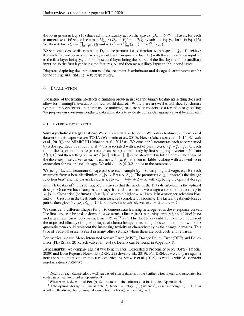
6.1 EXPERIMENTAL SETUP
Semi-synthetic data generation: We simulate data as follows. We obtain features, x, from a realdataset (in this paper we use TCGA (Weinstein et al., 2013), News (Johansson et al., 2016; Schwabet al., 2019)) and MIMIC III (Johnson et al., 2016))3. We consider 3 treatments each accompaniedby a dosage. Each treatment, w ∈ W , is associated with a set of parameters, vw1 ,v
w2 , vw3 . For each
run of the experiment, these parameters are sampled randomly by first sampling a vector, uwi , fromN (0,1) and then setting vwi = uwi /||uwi || where || · || is the standard Euclidean norm. The shape ofthe dose-response curve for each treatment, fw(x, d), is given in Table 1, along with a closed-formexpression for the optimal dosage. We add ε ∼ N (0, 0.2) noise to the outcomes.
We assign factual treatment-dosage pairs to each sample by first sampling a dosage, dw, for eachtreatment from a beta distribution, dw|x ∼ Beta(α, βw). The parameter α ≥ 1 controls the dosageselection bias4 and the parameter βw is set to βw = α−1
d∗w+ 2− α, with d∗w being the optimal dosage
for each treatment5. This setting of βw ensures that the mode of the Beta distribution is the optimaldosage. Once we have sampled a dosage for each treatment, we assign a treatment according towf |x ∼ Categorical(softmax(κf(x, dw)) where a higher κ will result in a stronger selection bias,and κ = 0 results in the treatments being assigned completely randomly. The factual treatment-dosagepair is then given by (wf , dwf
). Unless otherwise specified, we set κ = 2 and α = 2.
We consider 3 different shapes for fw to demonstrate learning heterogeneous dose-response curves.The first curve can be broken down into two terms, a linear (in d) increasing term (v1
1)Tx+12(v12)Txd
and a quadratic (in d) decreasing term −12(v13)Txd2. This first term could, for example, represent
the improved efficacy of higher dosages of chemotherapy in reducing the size of a tumour, while thequadratic term could represent the increasing toxicity of chemotherapy as the dosage increases. Thistype of trade-off presents itself in many other settings where there are both costs and rewards.
For metrics, we use Mean Integrated Square Error (MISE), Dosage Policy Error (DPE) and PolicyError (PE) (Silva, 2016; Schwab et al., 2019). Details can be found in Appendix F.
Benchmarks: We compare against two benchmarks: Generalized Propensity Score (GPS) (Imbens,2000) and Dose Reponse Networks (DRNet) (Schwab et al., 2019). For DRNets, we compare againstboth the standard model architecture described by Schwab et al. (2019) as well as with Wassersteinregularization (DRN-W).
3Details of each dataset along with suggested interpretations of the synthetic treatments and outcomes foreach dataset can be found in Appendix G
4When α = 1, βw = 1 and Beta(α, βw) reduces to the uniform distribution. See Appendix H.5If the optimal dosage is 0, we sample dw from 1− Beta(α, βw) where βw is set as though d∗w = 1. This
results in the dosage being sampled symmetrically for d∗w = 0 and d∗w = 1.
8

Under review as a conference paper at ICLR 2020
Treatment Dose-Response Optimal dosage
1 f1(x, d) = C((v11)
Tx+ 12(v12)
Txd− 12(v13)
Txd2) d∗1 =(v1
2)T x
2(v13)
T x
2 f2(x, d) = C((v21)
Tx+ sin(π(v22T x
v23T x
)d)) d∗2 =(v2
3)T x
2(v22)
T x
3 f3(x, d) = C((v31)
Tx+ 12d(d− b)2, where b = 0.75(v3
2)T x
(v33)
T x)
b3
if b ≥ 0.751 if b < 0.75
Table 1: Dose response curves used to generate semi-synthetic outcomes for patient features x. In theexperiments, we set C = 10. vw1 ,v
w2 , vw3 are the parameters associated with each treatment w.
As a baseline for comparison, we also use a standard multilayer perceptron (MLP) that takes as inputthe patient features, the treatment and dosage and estimates the patient outcome and a multitaskvariant (MLP-M) that has a designated head for each treatment. See Appendix E for details of thebenchmark models and their hyperparameter optimisation.
6.2 SOURCE OF GAIN
Before comparing against the benchmarks, we investigate how each component of our model affectsperformance. We start with a baseline model in which both the generator and discriminator consist ofa single fully connected network. One at a time, we add in the following components (cumulativelyuntil we reach our full model): (1) the supervised loss in Eq. 4 (+ LS), (2) multitask heads in thegenerator (+ Multitask), (3) hierarchical discriminator (+ Hierarchical) and (4) invariance/equivariancelayers in the treatment and dosage discriminators (+Inv/Eqv). We report the results in Table 2 forTCGA and News for all 3 error metrics (MISE, DPE and PE), computed over 30 runs.
TCGA News√MISE
√DPE
√PE
√MISE
√DPE
√PE
Baseline 4.18± 0.32 2.06± 0.16 1.93± 0.12 6.17± 0.27 6.97± 0.27 6.20± 0.21
+ LS 3.37± 0.11 1.14± 0.05 0.84± 0.05 4.51± 0.16 4.46± 0.12 4.40± 0.11
+ Multitask 3.15± 0.12 0.85± 0.05 0.67± 0.05 4.11± 0.11 4.33± 0.11 4.31± 0.11
+ Hierarchical 2.54± 0.05 0.36± 0.05 0.45± 0.05 4.07± 0.05 4.24± 0.11 4.17± 0.12
+ Inv/Eqv 1.89± 0.05 0.31± 0.05 0.25± 0.05 3.71± 0.05 4.14± 0.11 3.90± 0.05
Table 2: Source of gain analysis for our model. Metrics are reported as Mean ± Std.
We see that the addition of each component results in a performance improvement for our model,with the final row (which corresponds to our full model) demonstrating the best performance acrossboth datasets and for all metrics.
To further demonstrate the advantages of our hierarchical discriminator, in Fig. 5 we investigate howour hierarchical discriminator compares with a single network discriminator (all other componentsare included in both models, see Appendix B for details of the single discriminator) when we varythe hyperparameter nw on TCGA. Similar results for News can be found in Appendix I.1.
1 3 5 7 9 11 13 15 17 19Number of dosage samples
5
10
15
MIS
E
DRGAN - Hierarchical DRGAN - Single
(a)√
MISE
1 3 5 7 9 11 13 15 17 19Number of dosage samples
0
2
4
6
DPE
DRGAN - Hierarchical DRGAN - Single
(b)√
DPE
1 3 5 7 9 11 13 15 17 19Number of dosage samples
0
2
4
6
PE
DRGAN - Hierarchical DRGAN - Single
(c)√
PE
Figure 5: Performance of single vs. hierarchical discriminator when increasing the number of dosagesamples (nw) on TCGA dataset.
9

Under review as a conference paper at ICLR 2020
The performance of the single discriminator causes significant performance drops around nw = 9across all metrics. As previously noted, this is due to the dimension of the output space (which fornw = 9 is 27) being too large. Conversely, we see that our hierarchical discriminator shows muchmore stable performance even when nw = 19. We investigate in Appendix I.1 the hyperparameter λ.
6.3 BENCHMARKS COMPARISON
We now compare DRGAN against the benchmarks on our 3 semi-synthetic datasets. For Mimic, dueto the low number of samples available, we use only two treatments - 2 and 3. We report
√MISE and√
PE in Table 3, with results for√
DPE given in Appendix I.3. We see that DRGAN demonstratesa statistically significant improvement over every benchmark across all 3 datasets, confirming thatDRGAN is able to learn response-curves on top of very different underlying patient features.
Method TCGA News MIMIC√MISE
√PE
√MISE
√PE
√MISE
√PE
DRGAN 1.89± 0.05 0.25± 0.05 3.71± 0.05 3.90± 0.05 2.09± 0.12 0.32± 0.05
DRNet 3.64± 0.12 0.67± 0.05 4.98± 0.12 4.17± 0.11 4.45± 0.12 1.44± 0.05DRN-W 3.71± 0.12 0.63± 0.05 5.07± 0.12 4.56± 0.12 4.47± 0.12 1.37± 0.05GPS 4.83± 0.01 1.60± 0.01 6.97± 0.01 24.1± 0.05 7.39± 0.00 20.2± 0.01
MLP-M 3.96± 0.12 1.20± 0.05 5.17± 0.12 5.82± 0.16 4.97± 0.16 1.59± 0.05MLP 4.31± 0.05 0.97± 0.05 5.48± 0.16 6.45± 0.21 5.34± 0.16 1.65± 0.05
Table 3: Performance of individualized treatment-dose response estimation on three datasets. Boldindicates the method with the best performance for each dataset.
In Appendix I.4 we compare DRGAN with DRNET and GPS for an increasing number of treatments.
6.4 TREATMENT AND DOSAGE SELECTION BIAS
In this section, we assess the robustness of each method to varying treatment and dosage bias. Wereport results for
√MISE on TCGA here. For the other metrics see Appendix I.2. Fig. 6(a) shows the
performance of the 4 methods for κ between 0 (no bias) and 10 (strong bias). Fig. 6(b) shows theperformance for α between 1 (no bias) and 8 (strong bias). We see that our model shows consistentperformance, significantly outperforming the benchmark methods across the entire ranges of κ and α.
0 1 2 3 4 5 6 7 8 9 10Treatment assignment bias
1
2
3
4
5
6
7
MIS
E
DRGANMLP-M
DRNETGPS
(a) Treatment selection bias
1 2 3 4 5 6 7 8Dosage assignment bias
1
2
3
4
5
6
7
MIS
E
DRGANMLP-M
DRNETGPS
(b) Dosage selection bias
Figure 6: Performance of the 4 methods on datasets with varying bias levels.
7 CONCLUSION
In this paper we proposed a novel framework for estimating dose-response curves from observationaldata. Our method modified the GAN framework, introducing a novel hierarchical discriminator foruse in the dose-response setting. We also proposed novel architectures for the networks involved inour model and introduced a new semi-synthetic data simulation for use as a benchmark in this setting.On this data we demonstrated significant improvements over the benchmarks.
10

Under review as a conference paper at ICLR 2020
REFERENCES
Ahmed M Alaa and Mihaela van der Schaar. Bayesian inference of individualized treatment effectsusing multi-task gaussian processes. In Advances in Neural Information Processing Systems, pp.3424–3432, 2017.
Ahmed M Alaa, Michael Weisz, and Mihaela Van Der Schaar. Deep counterfactual networks withpropensity-dropout. arXiv preprint arXiv:1706.05966, 2017.
Susan Athey and Guido Imbens. Recursive partitioning for heterogeneous causal effects. Proceedingsof the National Academy of Sciences, 113(27):7353–7360, 2016.
James Bergstra and Yoshua Bengio. Random search for hyper-parameter optimization. Journal ofMachine Learning Research, 13(Feb):281–305, 2012.
Dimitris Bertsimas, Nathan Kallus, Alexander M Weinstein, and Ying Daisy Zhuo. Personalizeddiabetes management using electronic medical records. Diabetes Care, 40(2):210–217, 2017.
Hugh A Chipman, Edward I George, Robert E McCulloch, et al. BART: Bayesian additive regressiontrees. The Annals of Applied Statistics, 4(1):266–298, 2010.
Natalie Cook, Aaron R Hansen, Lillian L Siu, and Albiruni R Abdul Razak. Early phase clinicaltrials to identify optimal dosing and safety. Molecular Oncology, 9(5):997–1007, 2015.
Richard K Crump, V Joseph Hotz, Guido W Imbens, and Oscar A Mitnik. Nonparametric tests fortreatment effect heterogeneity. The Review of Economics and Statistics, 90(3):389–405, 2008.
Donna Döpp-Zemel and AB Johan Groeneveld. High-dose norepinephrine treatment: determinantsof mortality and futility in critically ill patients. American Journal of Critical Care, 22(1):22–32,2013.
Douglas Galagate. Causal Inference with a Continuous Treatment and Outcome: AlternativeEstimators for Parametric Dose-Response function with Applications. PhD thesis, 2016.
Ian Goodfellow, Jean Pouget-Abadie, Mehdi Mirza, Bing Xu, David Warde-Farley, Sherjil Ozair,Aaron Courville, and Yoshua Bengio. Generative adversarial nets. In Advances in NeuralInformation Processing Systems, pp. 2672–2680, 2014.
J Henry, Yuriy Pylypchuk, Talisha Searcy, and Vaishali Patel. Adoption of electronic health recordsystems among US non-federal acute care hospitals: 2008-2015. ONC Data Brief, 35:1–9, 2016.
Keisuke Hirano and Guido W Imbens. The propensity score with continuous treatments. AppliedBayesian Modeling and Causal Inference from Incomplete-Data Perspectives, 226164:73–84,2004.
Kosuke Imai and David A Van Dyk. Causal inference with general treatment regimes: Generalizingthe propensity score. Journal of the American Statistical Association, 99(467):854–866, 2004.
Guido W Imbens. The role of the propensity score in estimating dose-response functions. Biometrika,87(3):706–710, 2000.
Fredrik Johansson, Uri Shalit, and David Sontag. Learning representations for counterfactualinference. In International Conference on Machine Learning, pp. 3020–3029, 2016.
Alistair EW Johnson, Tom J Pollard, Lu Shen, H Lehman Li-wei, Mengling Feng, MohammadGhassemi, Benjamin Moody, Peter Szolovits, Leo Anthony Celi, and Roger G Mark. Mimic-iii, afreely accessible critical care database. Scientific Data, 3:160035, 2016.
Nathan Kallus. Recursive partitioning for personalization using observational data. In Proceedings ofthe 34th International Conference on Machine Learning-Volume 70, pp. 1789–1798. JMLR. org,2017.
Sheng Li and Yun Fu. Matching on balanced nonlinear representations for treatment effects estimation.In Advances in Neural Information Processing Systems, pp. 929–939, 2017.
11

Under review as a conference paper at ICLR 2020
Min Qian and Susan A Murphy. Performance guarantees for individualized treatment rules. Annalsof Statistics, 39(2):1180, 2011.
Peter M Rothwell, Nancy R Cook, J Michael Gaziano, Jacqueline F Price, Jill FF Belch, Maria CarlaRoncaglioni, Takeshi Morimoto, and Ziyah Mehta. Effects of aspirin on risks of vascular eventsand cancer according to bodyweight and dose: Analysis of individual patient data from randomisedtrials. The Lancet, 392(10145):387–399, 2018.
Donald B Rubin. Bayesianly justifiable and relevant frequency calculations for the applies statistician.The Annals of Statistics, pp. 1151–1172, 1984.
Patrick Schwab, Lorenz Linhardt, Stefan Bauer, Joachim M Buhmann, and Walter Karlen. Learningcounterfactual representations for estimating individual dose-response curves. arXiv preprintarXiv:1902.00981, 2019.
Uri Shalit, Fredrik D Johansson, and David Sontag. Estimating individual treatment effect: General-ization bounds and algorithms. In Proceedings of the 34th International Conference on MachineLearning-Volume 70, pp. 3076–3085. JMLR. org, 2017.
Claudia Shi, David M Blei, and Victor Veitch. Adapting neural networks for the estimation oftreatment effects. arXiv preprint arXiv:1906.02120, 2019.
Ricardo Silva. Observational-interventional priors for dose-response learning. In Advances in NeuralInformation Processing Systems, pp. 1561–1569, 2016.
Peter Spirtes. A tutorial on causal inference. 2009.
J Stoehlmacher, DJ Park, W Zhang, D Yang, S Groshen, S Zahedy, and HJ Lenz. A multivariate anal-ysis of genomic polymorphisms: Prediction of clinical outcome to 5-FU/Oxaliplatin combinationchemotherapy in refractory colorectal cancer. British Journal of Cancer, 91(2):344, 2004.
Moreno Ursino, Sarah Zohar, Frederike Lentz, Corinne Alberti, Tim Friede, Nigel Stallard, andEmmanuelle Comets. Dose-finding methods for Phase I clinical trials using pharmacokinetics insmall populations. Biometrical Journal, 59(4):804–825, 2017.
Stefan Wager and Susan Athey. Estimation and inference of heterogeneous treatment effects usingrandom forests. Journal of the American Statistical Association, 113(523):1228–1242, 2018.
Kyle Wang, Michael J Eblan, Allison M Deal, Matthew Lipner, Timothy M Zagar, Yue Wang,Panayiotis Mavroidis, Carrie B Lee, Brian C Jensen, Julian G Rosenman, et al. Cardiac toxicityafter radiotherapy for stage III non–small-cell lung cancer: Pooled analysis of dose-escalationtrials delivering 70 to 90 Gy. Journal of Clinical Oncology, 35(13):1387, 2017.
John N Weinstein, Eric A Collisson, Gordon B Mills, Kenna R Mills Shaw, Brad A Ozenberger, KyleEllrott, Ilya Shmulevich, Chris Sander, Joshua M Stuart, Cancer Genome Atlas Research Network,et al. The cancer genome atlas pan-cancer analysis project. Nature Genetics, 45(10):1113, 2013.
Liuyi Yao, Sheng Li, Yaliang Li, Mengdi Huai, Jing Gao, and Aidong Zhang. Representation learningfor treatment effect estimation from observational data. In Advances in Neural InformationProcessing Systems, pp. 2633–2643, 2018.
Jinsung Yoon, James Jordon, and Mihaela van der Schaar. GANITE: Estimation of individual-ized treatment effects using generative adversarial nets. International Conference on LearningRepresentations (ICLR), 2018.
Manzil Zaheer, Satwik Kottur, Siamak Ravanbakhsh, Barnabas Poczos, Ruslan R Salakhutdinov,and Alexander J Smola. Deep sets. In Advances in Neural Information Processing Systems, pp.3391–3401, 2017.
12
Under review as a conference paper at ICLR 2020
APPENDIX
A EXPANDED RELATED WORKS
Most methods for performing causal inference in the static setting focus on the scenario with twoor multiple treatment options and no dosage parameter. The approaches taken by such methods toestimate the treatment effects involve either building a separate regression model for each treatment(Stoehlmacher et al., 2004; Qian & Murphy, 2011; Bertsimas et al., 2017) or using the treatment as afeature and adjusting for the imbalance between the different treatment populations. The former doesnot generalise to the dosage setting due to the now infinite number of possible treatments available.In the latter case, methods for handling the selection bias involve propensity weighting (Crumpet al., 2008; Alaa et al., 2017; Shi et al., 2019), building sub-populations using tree based methods(Chipman et al., 2010; Athey & Imbens, 2016; Wager & Athey, 2018; Kallus, 2017) or buildingbalancing representations between patients receiving the different treatments (Johansson et al., 2016;Shalit et al., 2017; Li & Fu, 2017; Yao et al., 2018). An additional approach involves modelling thedata distribution of the factual and counterfactual outcomes (Alaa & van der Schaar, 2017; Yoonet al., 2018).
Silva (2016) leverages observational and interventional data to estimate the effects of discrete dosagesfor a single treatment. In particular, Silva (2016) uses observational data to construct a non-stationarycovariance function and develop a hierarchical Gaussian process prior to build a distribution over thedose response curve. Then, controlled interventions are employed to learn a non-parametric affinetransform to reshape this distribution. The setting in Silva (2016) differs significantly from ours aswe do not assume access to any interventional data.
13
Under review as a conference paper at ICLR 2020
B SINGLE DISCRIMINATOR MODEL
In the paper we developed a hierarchical discriminator and demonstrated that it performs significantlybetter than the single discriminator setup that we now describe in this section.
B.1 SINGLE DISCRIMINATOR
In the single model, we will aim to learn a single discriminator, D, that outputs P((Wf , Df ) =
(w, d)|X, Dw, Y) for each w ∈ W and d ∈ Dw. We will write Dw,d(·) to denote the output of Dthat corresponds to the treatment-dosage pair (w, d). We define the loss, LD, to be
LD(D;G) = −E[ ∑w∈W
∑d∈Dw
I{Tf=(w,d)} logDw,d(X, Y) + I{Tf 6=(w,d)} log(1−Dw,d(X, Y))
](19)
where the expectation is taken over X, {Dw}w∈W , Y,Wf and Df and we note that the dependenceon G is through Y. Our single discriminator will be trained to minimise this loss directly. Thegenerator GAN-loss, LG, is then defined by
LG(G) = −LD(D∗;G) (20)
where D∗ is the optimal discriminator given by minimising LD. The generator will be trained tominimise LG + λLS .
B.2 SINGLE DISCRIMINATOR ARCHITECTURE
y<latexit sha1_base64="(null)">(null)</latexit><latexit sha1_base64="(null)">(null)</latexit><latexit sha1_base64="(null)">(null)</latexit><latexit sha1_base64="(null)">(null)</latexit>
x<latexit sha1_base64="(null)">(null)</latexit><latexit sha1_base64="(null)">(null)</latexit><latexit sha1_base64="(null)">(null)</latexit><latexit sha1_base64="(null)">(null)</latexit>
Invariant layer
Invariant layer
Invariant layer
yw1<latexit sha1_base64="(null)">(null)</latexit><latexit sha1_base64="(null)">(null)</latexit><latexit sha1_base64="(null)">(null)</latexit><latexit sha1_base64="(null)">(null)</latexit>
yw2<latexit sha1_base64="(null)">(null)</latexit><latexit sha1_base64="(null)">(null)</latexit><latexit sha1_base64="(null)">(null)</latexit><latexit sha1_base64="(null)">(null)</latexit>
yw3<latexit sha1_base64="(null)">(null)</latexit><latexit sha1_base64="(null)">(null)</latexit><latexit sha1_base64="(null)">(null)</latexit><latexit sha1_base64="(null)">(null)</latexit>
f(y)<latexit sha1_base64="(null)">(null)</latexit><latexit sha1_base64="(null)">(null)</latexit><latexit sha1_base64="(null)">(null)</latexit><latexit sha1_base64="(null)">(null)</latexit>
Equivariant layer
Equivariant layer
Equivariant layer
Equivariant layer
Equivariant layer
Equivariant layer
p1,nw<latexit sha1_base64="(null)">(null)</latexit><latexit sha1_base64="(null)">(null)</latexit><latexit sha1_base64="(null)">(null)</latexit><latexit sha1_base64="(null)">(null)</latexit>
p1,1<latexit sha1_base64="(null)">(null)</latexit><latexit sha1_base64="(null)">(null)</latexit><latexit sha1_base64="(null)">(null)</latexit><latexit sha1_base64="(null)">(null)</latexit>
p2,1<latexit sha1_base64="(null)">(null)</latexit><latexit sha1_base64="(null)">(null)</latexit><latexit sha1_base64="(null)">(null)</latexit><latexit sha1_base64="(null)">(null)</latexit>
p2,nw<latexit sha1_base64="(null)">(null)</latexit><latexit sha1_base64="(null)">(null)</latexit><latexit sha1_base64="(null)">(null)</latexit><latexit sha1_base64="(null)">(null)</latexit>
p3,1<latexit sha1_base64="(null)">(null)</latexit><latexit sha1_base64="(null)">(null)</latexit><latexit sha1_base64="(null)">(null)</latexit><latexit sha1_base64="(null)">(null)</latexit>
p3,nw<latexit sha1_base64="(null)">(null)</latexit><latexit sha1_base64="(null)">(null)</latexit><latexit sha1_base64="(null)">(null)</latexit><latexit sha1_base64="(null)">(null)</latexit>
pij = P((Wf , Df ) = (wi, dwij ))
<latexit sha1_base64="(null)">(null)</latexit><latexit sha1_base64="(null)">(null)</latexit><latexit sha1_base64="(null)">(null)</latexit><latexit sha1_base64="(null)">(null)</latexit>
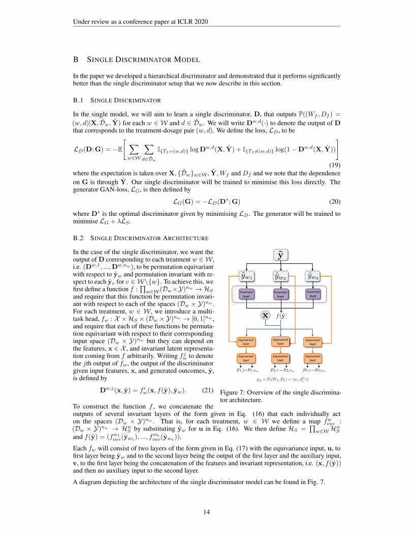
Figure 7: Overview of the single discrimina-tor architecture.
In the case of the single discriminator, we want theoutput of D corresponding to each treatment w ∈ W ,i.e. (Dw,1, ...,Dw,nw), to be permutation equivariantwith respect to yw and permutation invariant with re-spect to each yv for v ∈ W\{w}. To achieve this, wefirst define a function f :
∏w∈W(Dw×Y)nw → HS
and require that this function be permutation invari-ant with respect to each of the spaces (Dw × Y)nw .For each treatment, w ∈ W , we introduce a multi-task head, fw : X ×HS × (Dw ×Y)nw → [0, 1]nw ,and require that each of these functions be permuta-tion equivariant with respect to their correspondinginput space (Dw × Y)nw but they can depend onthe features, x ∈ X , and invariant latent representa-tion coming from f arbitrarily. Writing f jw to denotethe jth output of fw, the output of the discriminatorgiven input features, x, and generated outcomes, y,is defined by
Dw,j(x, y) = f iw(x, f(y), yw). (21)
To construct the function f , we concatenate theoutputs of several invariant layers of the form given in Eq. (16) that each individually acton the spaces (Dw × Y)nw . That is, for each treatment, w ∈ W we define a map fwinv :(Dw × Y)nw → HwS by substituting yw for u in Eq. (16). We then define HS =
∏w∈W HwS
and f(y) = (fw1inv(yw1), ..., fwk
inv(ywk)).
Each fw will consist of two layers of the form given in Eq. (17) with the equivariance input, u, tofirst layer being yw and to the second layer being the output of the first layer and the auxiliary input,v, to the first layer being the concatenation of the features and invariant representation, i.e. (x, f(y))and then no auxiliary input to the second layer.
A diagram depicting the architecture of the single discriminator model can be found in Fig. 7.
14

Under review as a conference paper at ICLR 2020
C COUNTERFACTUAL GENERATOR PSEUDO-CODE
Algorithm 1 Training of the generator in DRGAN1: Input: dataset C = {(xi, tif , yif ) : i = 1, ..., N}, batch size nmb, number of dosages per
treatment nd, number of discriminator updates per iteration nD, number of generator updates periteration nG, dimensionality of noise nz , learning rate α
2: Initialize: θG, θW , {θw}w∈W3: while G has not converged do
Discriminator updates4: for i = 1, ..., nD do5: Sample (x1, (w1, d1), y1), ..., (xnmb
, (wnmb, dnmb
), ynmb) from C
6: Sample generator noise zj = (zj1, ..., zjnz
) from Unif([0, 1]nz ) for j = 1, ..., nmb7: for w ∈ W do8: for j = 1, ..., nmb do9: Sample Dj
w = (dw,j1 , ..., dw,jnd) independently and uniformly from (Dw)nd
10: Set yjw according to Eq. 511: Calculate gradient of dosage discriminator loss
gw ← ∇θw −
∑{j:wj=w}
nd∑k=1
I{dj=dw,jk } logDw(xj , y
jw) + I{dj 6=dw,j
k } log(1−Dw(xj , yjw))
12: Update dosage discriminator parameters θw ← θw + αgw13: Set yj = (yjw)w∈W14: Calculate gradient of treatment discriminator loss
gW ← ∇θW −
nmb∑j=1
∑w∈W
I{wj=w} logDW(xj , yj) + I{wj 6=w} log(1−DW(xj , yj))
15: Update treatment discriminator parameters θW ← θW + αgW
Generator updates16: for i = 1, ..., nG do17: Sample (x1, (w1, d1), y1), ..., (xnmb
, (wnmb, dnmb
), ynmb) from C
18: Sample generator noise zj = (zj1, ..., zjnz
) from Unif([0, 1]nz ) for j = 1, ..., nmb19: Sample (Dj
w)w∈W from Πw∈W(Dw)nd for j = 1, ..., nmb20: Set y according to Eq. 521: Calculate gradient of generator loss
gG ← ∇θG
[nmb∑j=1
∑w∈W
nd∑l=1
I{wj=w,dj=dw,jl } log(Dw
W(xj , yj)w ×Dlw(xj , y
jw)l)
+I{wj 6=w,dj 6=dw,jl } log(1− (Dw
W(xj , yj)×Dlw(xj , y
jw)))
]22: Update generator parameters θG ← θG + αgG23: Output: G
15

Under review as a conference paper at ICLR 2020
D INFERENCE NETWORK
To generate dose-response curves for new samples, we learn an inference network, I : X× T → Y .This inference network is trained using the original dataset and the learned counterfactual generator.As with the training of the generator and discriminator, we train using a random set of dosages, Dw.The loss is given by
LI(I) = E
[ ∑w∈W
∑d∈Dw
(Y (w, d)− I(X, (w, d)))2
], (22)
where Y (w, d) is Yf if Tf = (w, d) or given by the generator if Tf 6= (w, d). The expectation istaken over X, Tf , Yf ,Z and Dw.
D.1 PSEUDO-CODE FOR TRAINING THE INFERENCE NETWORK
Algorithm 2 Training of the inference network in DRGAN1: Input: dataset C = {(xi, tif , yif ) : i = 1, ..., N}, trained generator G, batch size nmb, number
of dosages per treatment nd, dimensionality of noise nz , learning rate α2: Initialize: θI ,3: while I has not converged do4: Sample (x1, (w1, d1), y1), ..., (xnmb
, (wnmb, dnmb
), ynmb) from C
5: Sample generator noise zj = (zj1, ..., zjnz
) from Unif([0, 1]nz ) for j = 1, ..., nmb6: for j = 1, ..., nmb do7: for w ∈ W do8: Sample Dj
w = (dw,j1 , ..., dw,jnd) independently and uniformly from (Dw)nd
9: Set yjw according to Eq. 5 510: Calculate gradient of inference network loss
gI ← ∇θI
[nmb∑j=1
∑w∈W
nd∑l=1
(yjw)l − I(xj , (w, dw,jl ))2
]
11: Update inference network parameters θI ← θI + αgI12: Output: I
16

Under review as a conference paper at ICLR 2020
E BENCHMARKS
We use the publicly available GitHub implementation of DRNet provided by Schwab et al. (2019):https://github.com/d909b/drnet. Moreover, we also used a GPS implementation similarto the one from https://github.com/d909b/drnetwhich uses the causaldrfR package(Galagate, 2016). More spcifically, the GPS implementation uses a normal treatment model, a lineartreatment formula and a 2-nd degree polynomial for the outcome. Moreover, for the TCGA and Newsdatasets, we performed PCA and only used the 50 principal components as input to the GPS model toreduce computational complexity.
Hyperparameter optimization: The validation split of the dataset is used for hyperparameteroptimization. For the DRNet benchmarks we use the same hyperparameter optimization proposed bySchwab et al. (2019) with the hyperparameter search ranges described in Table 4. For DRGAN, weuse the hyperparameter optimization method proposed in GANITE (Yoon et al., 2018), where weuse the complete dataset from the counterfactual generator to evaluate the MISE on the inferencenetwork. We perform a random search (Bergstra & Bengio, 2012) for hyperparameter optimizationover the search ranges in Table 5. For a fair comparison, for the MLP-M model we used the samearchitecture used in the inference network of DRGAN. Similarly, for the MLP model we use thesame architecture as for the MLP-M, but without the multitask heads.
Hyperparameter Search range
Batch size 32, 64, 128Number of units per hidden layer 24, 48, 96, 192Number of hidden layers 2, 3Dropout percentage 0.0, 0.2Imbalance penalty weight∗ 0.1, 1.0, 10.0
Fixed
Number of dosage strata E 5
Table 4: Hyperparameters search range for DRNet. *: For the DRNet model using Wassersteinregularization only.
Hyperparameter Search range
Batch size 64, 128, 256Number of units per hidden layer 32, 64, 128Size of invariant and equivariant representations 16, 32, 64, 128
Fixed
Number of hidden layers per multitask head 2Number of dosage samples 5λ 1Optimization Adam Moment Optimization
Table 5: Hyperparameters search range for DRGAN.
17

Under review as a conference paper at ICLR 2020
F METRICS
The Mean Integrated Square Error (MISE) measures how well the models estimates the patientoutcome across the entire dosage space:
MISE =1
N
1
k
∑w∈W
N∑i=1
∫Dw
(yi(w, u)− yi(w, u)
)2du . (23)
In addition to this, we also compute the mean dosage policy error (DPE) (Schwab et al., 2019) toassess the ability of the model to estimate the optimal dosage point for every treatment for eachindividual:
DPE =1
N
1
k
∑w∈W
N∑i=1
(yi(w, d∗w)− yi(w, d∗w)
)2, (24)
where d∗w is the true optimal dosage and d∗w is the optimal dosage identified by the model. Theoptimal dosage points for a model are computed using SciPy’s implementation of Sequential LeastSQuares Programming.
Finally, we compute the mean policy error (PE) (Schwab et al., 2019) which compares the outcomeof the true optimal treatment-dosage pair to the outcome of the optimal treatment-dosage pair asselected by the model:
PE =1
N
N∑i=1
(yi(w∗, d∗w)− yi(w∗, d∗w)
)2, (25)
where w∗ is the true optimal treatment and w∗ is the optimal treatment identified by the model. Theoptimal treatment-dosage pair for a model is selected by first computing the optimal dosage for eachtreatment and then selecting the treatment with the best outcome for its optimal dosage.
Each of these metrics are computed on a held out test-set.
18
Under review as a conference paper at ICLR 2020
G DATASET DESCRIPTIONS
TCGA: The TCGA dataset consists of gene expression measurements for cancer patients (Wein-stein et al., 2013). There are 9659 samples for which we used the measurements from the 4000most variable genes. The gene expression data was log-normalized and each feature was scaledin the [0, 1] interval. Moreover, for each patient, the features x were scaled to have norm 1. Wegive meaning to our treatments and dosages by considering the treatment as being chemother-apy/radiotherapy/immunotherapy and their corresponding dosages. The outcome can be thought ofas the risk of cancer recurrence (Schwab et al., 2019).
News: The News dataset consists of word counts for news items. We extracted 10000 samples eachwith 2858 features. As in (Johansson et al., 2016; Schwab et al., 2019), we give meaning to ourtreatments and dosages by considering the treatment as being the viewing device (e.g. phone, tabletetc.) used to read the article and the dosage as being the amount of time spent reading it. The outcomecan be thought of as user satisfaction.
MIMIC III: The Medical Information Mart for Intensive Care (MIMIC III) (Johnson et al., 2016)database consists of observational data from patients in the ICU. We extracted 3000 patients thatreceive antibiotics treatment and we used as features 9 clinical covariates measured during the dayof ICU admission. Again, the features were scaled in the [0, 1] interval. In this setting, we canconsidered as treatments the different antibiotics and their corresponding dosages.
For a summary description of the datasets, see table 6. The datasets are split into 64/16/20% fortraining, validation and testing respectively. The validation dataset is used for hyperparameteroptimization.
TCGA News MIMIC
Number of samples 9659 10000 3000Number of features 4000 2858 9Number of treatments 3* 3 2
Table 6: Summary description of datasets. *: for our final experiment in Appendix I.4 we increasethe number of treatments in TCGA to 6 and 9.
H DOSAGE BIAS
In order to create dosage-assignment bias in our dataset, we assign dosages according to dw|x ∼Beta(α, βw). The selection bias is controlled by the parameter α ≥ 1. When we set βw = α−1
d∗w+2−α
(which ensures that the mode of our distribution is d∗w), we can write the variance of dw in terms of αand d∗w as follows
Var(dw) =
α2−αd∗w
+ 2α− α2
(α−1d∗w+ 2)2(α−1d∗w
+ 3)≈ cα2
dα3. (26)
We see that the variance of our Beta distribution therefore decreases with α, resulting in the sampleddosages being closer to the optimal dosage, thus resulting in higher dosage-selection bias. In additionwe note that the Beta(1, 1) distribution is in fact the uniform distribution, corresponding to thedosages being sampled independently of the patient features, resulting in no selection bias whenα = 1.
19
Under review as a conference paper at ICLR 2020
I ADDITIONAL RESULTS
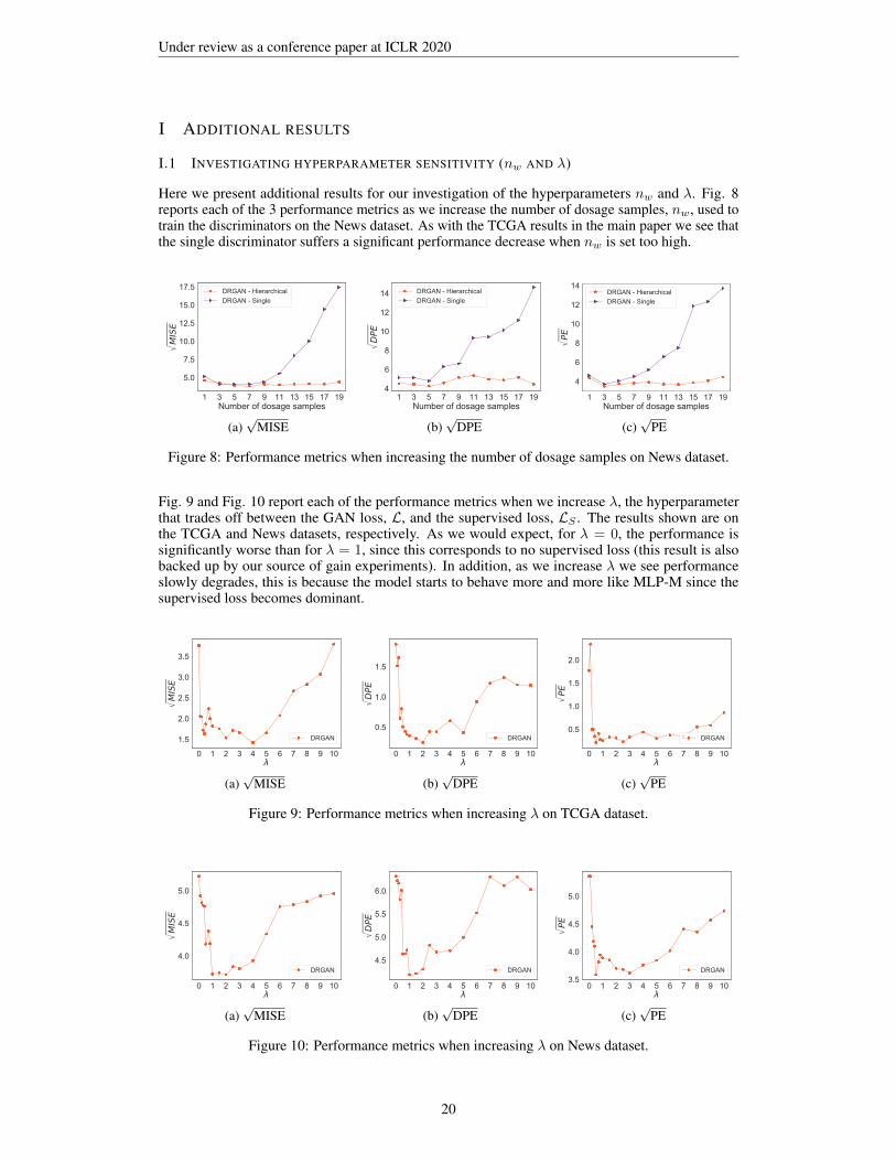
I.1 INVESTIGATING HYPERPARAMETER SENSITIVITY (nw AND λ)
Here we present additional results for our investigation of the hyperparameters nw and λ. Fig. 8reports each of the 3 performance metrics as we increase the number of dosage samples, nw, used totrain the discriminators on the News dataset. As with the TCGA results in the main paper we see thatthe single discriminator suffers a significant performance decrease when nw is set too high.
1 3 5 7 9 11 13 15 17 19Number of dosage samples
5.0
7.5
10.0
12.5
15.0
17.5
MIS
E
DRGAN - Hierarchical DRGAN - Single
(a)√
MISE
1 3 5 7 9 11 13 15 17 19Number of dosage samples
4
6
8
10
12
14
DPE
DRGAN - Hierarchical DRGAN - Single
(b)√
DPE
1 3 5 7 9 11 13 15 17 19Number of dosage samples
4
6
8
10
12
14
PE
DRGAN - Hierarchical DRGAN - Single
(c)√
PE
Figure 8: Performance metrics when increasing the number of dosage samples on News dataset.
Fig. 9 and Fig. 10 report each of the performance metrics when we increase λ, the hyperparameterthat trades off between the GAN loss, L, and the supervised loss, LS . The results shown are onthe TCGA and News datasets, respectively. As we would expect, for λ = 0, the performance issignificantly worse than for λ = 1, since this corresponds to no supervised loss (this result is alsobacked up by our source of gain experiments). In addition, as we increase λ we see performanceslowly degrades, this is because the model starts to behave more and more like MLP-M since thesupervised loss becomes dominant.
0 1 2 3 4 5 6 7 8 9 10
1.5
2.0
2.5
3.0
3.5
MIS
E
DRGAN
(a)√
MISE
0 1 2 3 4 5 6 7 8 9 10
0.5
1.0
1.5
DPE
DRGAN
(b)√
DPE
0 1 2 3 4 5 6 7 8 9 10
0.5
1.0
1.5
2.0
PE
DRGAN
(c)√
PE
Figure 9: Performance metrics when increasing λ on TCGA dataset.
0 1 2 3 4 5 6 7 8 9 10
4.0
4.5
5.0
MIS
E
DRGAN
(a)√
MISE
0 1 2 3 4 5 6 7 8 9 10
4.5
5.0
5.5
6.0
DPE
DRGAN
(b)√
DPE
0 1 2 3 4 5 6 7 8 9 103.5
4.0
4.5
5.0
PE
DRGAN
(c)√
PE
Figure 10: Performance metrics when increasing λ on News dataset.
20
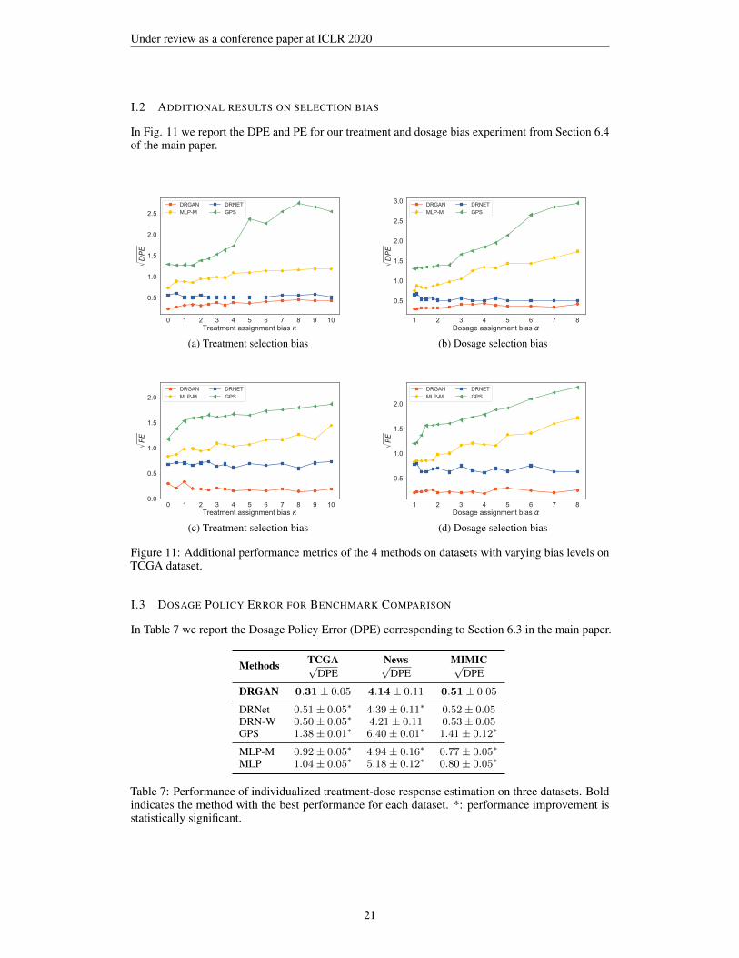
Under review as a conference paper at ICLR 2020
I.2 ADDITIONAL RESULTS ON SELECTION BIAS
In Fig. 11 we report the DPE and PE for our treatment and dosage bias experiment from Section 6.4of the main paper.
0 1 2 3 4 5 6 7 8 9 10Treatment assignment bias
0.5
1.0
1.5
2.0
2.5
DPE
DRGANMLP-M
DRNETGPS
(a) Treatment selection bias
1 2 3 4 5 6 7 8Dosage assignment bias
0.5
1.0
1.5
2.0
2.5
3.0
DPE
DRGANMLP-M
DRNETGPS
(b) Dosage selection bias
0 1 2 3 4 5 6 7 8 9 10Treatment assignment bias
0.0
0.5
1.0
1.5
2.0
PE
DRGANMLP-M
DRNETGPS
(c) Treatment selection bias
1 2 3 4 5 6 7 8Dosage assignment bias
0.5
1.0
1.5
2.0
PEDRGANMLP-M
DRNETGPS
(d) Dosage selection bias
Figure 11: Additional performance metrics of the 4 methods on datasets with varying bias levels onTCGA dataset.
I.3 DOSAGE POLICY ERROR FOR BENCHMARK COMPARISON
In Table 7 we report the Dosage Policy Error (DPE) corresponding to Section 6.3 in the main paper.
Methods TCGA News MIMIC√DPE
√DPE
√DPE
DRGAN 0.31± 0.05 4.14± 0.11 0.51± 0.05
DRNet 0.51± 0.05∗ 4.39± 0.11∗ 0.52± 0.05DRN-W 0.50± 0.05∗ 4.21± 0.11 0.53± 0.05GPS 1.38± 0.01∗ 6.40± 0.01∗ 1.41± 0.12∗
MLP-M 0.92± 0.05∗ 4.94± 0.16∗ 0.77± 0.05∗
MLP 1.04± 0.05∗ 5.18± 0.12∗ 0.80± 0.05∗
Table 7: Performance of individualized treatment-dose response estimation on three datasets. Boldindicates the method with the best performance for each dataset. *: performance improvement isstatistically significant.
21
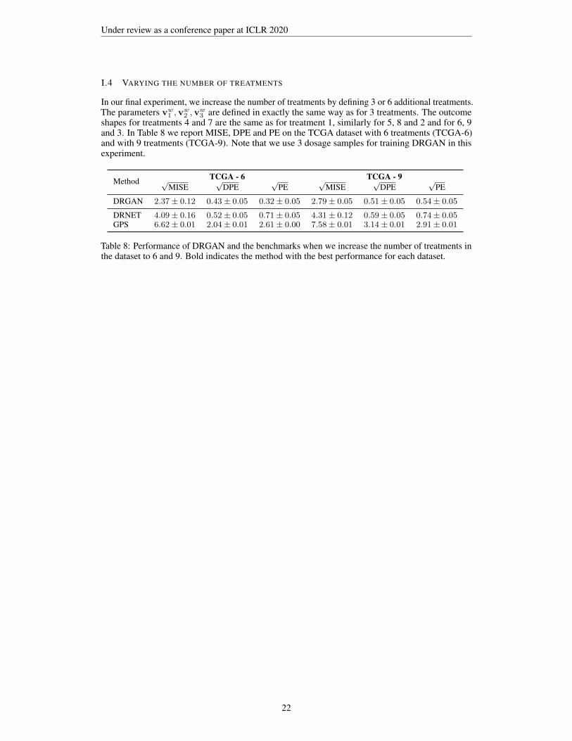
Under review as a conference paper at ICLR 2020
I.4 VARYING THE NUMBER OF TREATMENTS
In our final experiment, we increase the number of treatments by defining 3 or 6 additional treatments.The parameters vw1 ,v
w2 ,v
w3 are defined in exactly the same way as for 3 treatments. The outcome
shapes for treatments 4 and 7 are the same as for treatment 1, similarly for 5, 8 and 2 and for 6, 9and 3. In Table 8 we report MISE, DPE and PE on the TCGA dataset with 6 treatments (TCGA-6)and with 9 treatments (TCGA-9). Note that we use 3 dosage samples for training DRGAN in thisexperiment.
Method TCGA - 6 TCGA - 9√MISE
√DPE
√PE
√MISE
√DPE
√PE
DRGAN 2.37± 0.12 0.43± 0.05 0.32± 0.05 2.79± 0.05 0.51± 0.05 0.54± 0.05
DRNET 4.09± 0.16 0.52± 0.05 0.71± 0.05 4.31± 0.12 0.59± 0.05 0.74± 0.05GPS 6.62± 0.01 2.04± 0.01 2.61± 0.00 7.58± 0.01 3.14± 0.01 2.91± 0.01
Table 8: Performance of DRGAN and the benchmarks when we increase the number of treatments inthe dataset to 6 and 9. Bold indicates the method with the best performance for each dataset.
22