Individual mobility: From conventional to electric carspublications.jrc.ec.europa.eu/repository/bitstream/... · data were collected through a Web-based travel diary, 24 hours per

Forename(s) Surname(s)

Alberto V. Donati Panagiota Dilara*

Christian Thiel Alessio Spadaro Dimitrios Gkatzoflias Yannis Drossinos European Commission, Joint Research Centre, I-21027 Ispra (VA), Italy *Current address: European Commission, DG GROW, B-1049 Brussels, Belgium 2015

Individual mobility:

From conventional to electric cars

Report EUR 27468 EN

European Commission

Joint Research Centre

Institute for Energy and Transport

Contact information

Yannis Drossinos

Address: Joint Research Centre, Via Enrico Fermi 2749, TP 441, I-21027 Ispra (VA), Italy

E-mail: [email protected]

Tel.: +39 0332 78 5387

Fax: +39 0332 78 5236

JRC Science Hub

http://ses.jrc.ec.europa.eu

Legal Notice

This publication is a Science and Policy Report by the Joint Research Centre, the European Commission’s in-house science service.

It aims to provide evidence-based scientific support to the European policy-making process. The scientific output expressed does

not imply a policy position of the European Commission. Neither the European Commission nor any person acting on behalf of the

Commission is responsible for the use which might be made of this publication.

All images © European Union 2015

JRC97690

EUR 27468 EN

ISBN 978-92-79-51894-2 (PDF)

ISBN 978-92-79-51895-9 (print)

ISSN 1831-9424 (online)

ISSN 1018-5593 (print)

doi:10.2790/405373 (online)

Luxembourg: Publications Office of the European Union, 2015

© European Union, 2015

Reproduction is authorised provided the source is acknowledged.

Printed in Italy

Abstract

The aim of this report is twofold. First, to analyse individual (driver) mobility data to obtain fundamental statistical parameters of driving patterns for both conventional and electric vehicles. In doing so, the information contained in large mobility datasets is condensed into compact and concise descriptions through modelling observed (experimental) distributions of mobility variables by expected theoretical distributions. Specifically, the stretched exponential distribution is shown to model rather accurately the distribution of single-trips and their duration, and the scale-invariant power-law with exponential cut-off the daily mobility length, the distance travelled per day. We argue that the theoretical-distribution parameters depend on the road-network topology, terrain topography, traffic, points of interest, and individual activities. Data from conventional vehicles suggest three approximate daily driving patterns corresponding to weekday, Saturday and Sunday driving, the latter two being rather similar. Work trips were found to be longer than average and of longer duration. The second aim is to ascertain, via the limited electric-vehicle data available from the EU-funded Green eMotion project, whether the behaviour of drivers of conventional vehicles differs from the behaviour of drivers of electric vehicles. The data suggest that electric vehicles are driven for shorter distances and shorter duration. Data from the Green eMotion project showed that the median real-life energy consumption of a typical segment A, small-sized, electric car, for example the Mitsubishi i-MiEV and its variants, is 186 Wh/km with a spread of 55 Wh/km. The real-driving energy consumption (per km) was determined to be approximately 38% higher than the type-approved consumption. Moreover, we found considerable dependence of the energy consumed on the ambient temperature. The median winter energy consumption per kilometre was higher than the median summer consumption by approximately 40%. The data presented in this report can be fundamental for subsequent analyses of infrastructure requirements for electric vehicles and assessments of their potential contribution to energy, transport, and climate policy objectives.

1

Contents

1. Introduction ....................................................................................................................................................... 2

2. Datasets ............................................................................................................................................................. 3

3. Conventional vehicles ........................................................................................................................................ 4

3.1 Floating-car data ............................................................................................................................... 4

3.1.1 Trip Distance ..................................................................................................................................... 6

3.1.2 Daily mobility distance .................................................................................................................... 10

3.1.3 Number of daily trips ...................................................................................................................... 14

3.1.4 Trip starting time and trip duration ................................................................................................ 15

3.1.5 Work trips ....................................................................................................................................... 17

3.1.6 Average trip speed, motion speed, and segment speed ................................................................ 18

3.1.7 Parking ............................................................................................................................................ 19

3.1.8 Discussion ....................................................................................................................................... 20

3.2 Survey data ..................................................................................................................................... 22

4. Electric vehicles: Green eMotion project ........................................................................................................ 23

4.1 Mobility characteristics ................................................................................................................... 24

4.2 Energy consumption and charging ................................................................................................. 28

4.3 Driving range ................................................................................................................................... 36

5. Comparison and discussion ............................................................................................................................. 38

6. Conclusions ...................................................................................................................................................... 41

7. Acknowledgments ........................................................................................................................................... 43

8. References ....................................................................................................................................................... 44

Appendix A............................................................................................................................................................... 46

Appendix B ............................................................................................................................................................... 62

2

1. Introduction Road transport, a key component of economic development and human welfare, plays a growing role in world

energy use and emissions of greenhouse gases. In 2010, the transport sector was responsible for

approximately 23% of total energy-related carbon dioxide emissions, a potent greenhouse gas. Greenhouse

gas (GHG) emissions from the transport sector have more than doubled since 1970, increasing at a faster rate

than any other energy end-use sector to reach 7.0Gt carbon-dioxide equivalent in 2010. Around 80% of this

increase came from road vehicles. The final energy consumption for transport reached 28% of the total end-

use energy in 2010, of which around 40% was used for urban transport [1]. In the European Union, road

transport contributes one-fifth of EU’s total emissions of carbon dioxide. Emissions in 2012, even though they

fell by 3.3%, were still 20.5% higher than in 1990. Light-duty vehicles, cars and vans, produce approximately

15% of the EU’s emissions of carbon dioxide [2]. Moreover, transport in Europe is 94 % dependent on oil, 84 %

of it imported, leading to a financial cost of EUR 1 billion per day and significant dependence on importing oil

with the consequent threat to the EU’s security of energy supply [3].

Emissions from road transport, be they gaseous like ozone and nitrogen oxides or in particulate form, for

example, combustion-generated nanoparticles, influence air quality in cities. Numerous epidemiological and

toxicological studies have associated urban air quality and air pollution, including particular matter, with

adverse health effects [4].

Therefore, the use of fossil fuels has significant repercussions on the environment, public health, and political

decisions. Burning fossil fuels leads to (i) important detrimental effects on the environment (GHG emissions

and climate change); (ii) deterioration of urban air quality and associated human health effects, causing

increasing environmental and human costs; and (iii) it is considered a threat to the EU security of energy

supply.

The European Commission regards alternative fuels an important option to sustainable mobility in Europe. The

Clean Power for Transport package, adopted in 2013, aims to foster the development of a single market for

alternative fuels for transport in Europe. It contains a Communication laying out a comprehensive European

alternative fuels strategy [COM(2013)17] for the long-term substitution of oil as an energy source in all modes

of transport. The Directive on the deployment of alternative fuels infrastructure (2014/94/EU) requires

Member States to develop national policy frameworks for the market development of alternative fuels and

their infrastructure, among other elements. However, a detailed analysis of the way alternative-fuel vehicles

move and consume energy is necessary to understand the needs for a European-level infrastructure.

Herein, we analyse real-life data for conventional and electric vehicles as they move in various European cities

and areas. The conventional-vehicle data were collected by on-board data loggers or from specific-purpose

surveys. Electric-vehicle data have become available only recently, since only in the last few years large

electric-vehicle demonstration projects have been funded, as the Zem2all in Malaga (ES) or the Switch EV in

Newcastle (UK). A brief description of both projects may be found in Ref. [5]. The data analysed in this report

were obtained from the Green eMotion Project [5] that generated a wealth of data on how drivers use electric

vehicles, their driving and parking patterns, and real-life energy consumption of electric vehicles in Europe.

We provide generic modelling of individual (driver) mobility, by conventional or by electric vehicles, while at

the same time we analyse consumption patterns of electric vehicles. These models may be used to study the

needs for infrastructure in the Member States and, thence, to support the elaboration of the national policy

frameworks. The models and data summarized in this report can be used as a basis and first step to analyse

the necessary electricity infrastructure investments under significant electric-vehicle deployment scenarios.

For example, estimated energy consumption of observed (recorded) trips, aggregated and appropriately

scaled to the population of the circulating electric vehicles, provide estimates of city-wide energy needs.

Clustering techniques may be used to identify classes of driving-behaviour and related patterns that provide

3

insights on daily activities. Such characterization of drivers’ behaviour could be used profitably to decide the

optimal placement of charging stations, as well as their most cost-efficient number.

2. Datasets Three distinct datasets, containing complementary information on urban mobility characteristics, were

analysed. Two datasets, Floating-car and Survey data, were collected for conventional vehicles (powered by

internal combustion engines), and one for the electric vehicles that participated in the Green eMotion (GeM)

project.

The Floating-car data [6,7] were purchased from the company Octo Telematics by the JRC to analyse

conventional mobility behaviour, namely to identify patterns and aspects of human mobility in urban areas

under different conditions (traffic, road-network topology). The database contains a large amount of

information on conventional (internal combustion engine) private and commercial vehicles: the mobility data

were collected in two medium-sized Italian cities (Modena and Florence) in May 2011. The data were acquired

via the Clear Box technology, whereby a GPS device (used to localize the vehicle) is connected to a remote

server via GSM. As described in Ref. [7], the initial dataset contains data collected from about 52,834

(Modena) and 40,459 (Florence) conventional vehicles, a well-mixed random sample that represents 12%

(Modena) and 5.9% (Florence) of the circulating fleet. As the primary interest in the analyses of the

conventional-vehicle data is urban mobility, the data were filtered to eliminate vehicles driven for more than

50% of the trips outside the respective province. This filtering resulted in approximately 48 million valid

sampled events arising from approximately 29 thousand vehicles. For each recorded event, the GPS device

automatically acquires: timestamp (date and time), GPS position and signal strength, engine state (start,

motion, stop), instantaneous speed, direction of motion, and distance travelled from the previous recorded

event. The records were transmitted to the server every 2 km [6]. These Floating-car data, and the resulting

travel behaviour in the two medium-size Italian cities, were extensively analysed in Refs. [7-9], albeit from a

different perspective.

The Survey data [10-12] were collected by the Institute of Energy and Transport of the JRC in collaboration

with TRT (Trasporti e Territorio Srl) and Ipsos Public Affairs Srl. A JRC initiative was launched in the spring of

2012 to investigate the behaviour of European car drivers, as described in detail in Refs. [11,12]. The survey

data were collected through a Web-based travel diary, 24 hours per day, 7 days a week. The database contains

trip diaries for six European countries (France, Germany, Italy, Poland, Spain, and UK) of about 600 individuals

in each country. The sample, for each country, was chosen to guarantee the necessary statistical homogeneity

and to be representative of the population in terms of age, gender, geographical area, population density,

education, and occupational status. The data were collected to complement data of national surveys that, with

the exception of UK and Germany, were considered insufficient to compare driving patterns across Europe.

Individuals logged the information at the end of each trip, for a total of about 40,000 trips for 3,500

conventional cars; a total of about 122,000 diary entries were recorded, covering a period of about 4 months

(from February to May 2012, even though for any individual vehicle the usual span was about 2 months). No

information on the location of the vehicles was recorded.

The Green eMotion data [5,13] were provided to the JRC by IREC (Catalonia Institute for Energy Research) as

part of a collaboration initiated at the end of 2013. The Green eMotion database contains data about the

mobility of electric vehicles of various types (cars, motorcycles, and transporters), and powertrain

technologies: Battery Electric Vehicle (BEV), and Plug-in Hybrid Electric Vehicle (PHEV). Most of the BEV cars

were Mitsubishi i-MiEV or its versions targeted to the European market–Peugeot iOn and Citroen C-Zero - and

a limited number of Think City (mainly in Spain). The vehicles were driven in 11 different Demonstration

(Demo) Regions, representing various cities in six European countries (Denmark, France, Germany, Ireland,

Italy, and Sweden). As the data were occasionally incomplete, we proposed appropriate guidelines for data

4

collection and reporting for European electro-mobility projects [14]. The database contains both static and

dynamic data. Static data refer to the vehicle (type, engine technology, usage) and to the charging station

(number of charging points per station, power output, location in GPS coordinates). The static information was

usually updated every 6 months. The dynamic data are the start and end times of a trip, and recharging

information: they were recorded by on-board loggers for the period March 2011 to December 2013. From the

full database, we extracted the travel distance per trip, vehicle energy consumption, and recharge time,

energy, and power. Unfortunately, vehicle location was reported (GPS location) only at the beginning and the

end of a trip: no intermediate route information was available to allow us to extract instantaneous speed or

acceleration. The number of electric vehicles (cars, motorcycles, and transporters) we analysed is 457, while

those driven for at least one trip were 357, all of them battery-electric cars. The total number of trips analysed

is 65,799.

A condensed version of this report was included in the Deliverable D1.10, “European global analysis on the

electro-mobility performance” of the Green eMotion project [5].

3. Conventional vehicles The analysis of mobility data of conventional vehicles is of importance since it allows the identification of

general principles of individual (driver) mobility and the associated driving-behaviour patterns. Such

information may suggest actions to be taken to allow a smooth transition from internal-combustion powered

to electrically-powered vehicles.

The following list presents the variables that were analysed: some of them were subdivided by day of the

week, or aggregated per working and weekend day. Distributions of some of them were also studied. The

variables are:

1. Trip distance. A trip is defined as a sequence of events (GPS records) that starts with a signal of

“engine on” and end with a signal “engine off”;

2. Trip start time, trip duration, total time between the start and end of a trip;

3. Distance and duration of work trips, e.g. trips that can be related to a regularly performed activity

that will be referred to as “work”. They were defined as trips that consisted of two contiguous legs,

the destination of the first coinciding with the origin of the second and vice versa, separated by a

parking time between 7.5 to 9 hours;

4. Average trip speed and average motion speed, the latter being the average trip speed obtained by

removing the time a vehicle was motionless from the total trip duration. The averages were

calculated by dividing the total trip distance either by the trip duration (average trip speed) or by the

time the vehicle was in motion (average motion speed). We also calculated segment speeds, the

average speed calculated from one GPS record to the next by dividing the reported distance travelled

by the time difference between the two consequently recorded events;

5. Parking duration, aggregated per week day, per working day, and per weekend day;

6. Daily mobility distance, the total distance travelled per day, and the daily number of trips;

7. Trip distance travelled before a stop of a given duration.

3.1 Floating-car data The Floating-car data consisted of a collection of GPS signals of private and commercial (a much smaller fraction) vehicles for two medium-size Italian cities, Modena and Florence, collected in May 2011. The

5

monitored vehicles of the cleaned database, i.e., after removal of vehicles that travelled more than 50% of the trips outside the respective province, represented 3.7% (16,254 vehicles, Modena) ad 1.8% (12,475 vehicles, Florence) of the vehicles registered in these provinces at that time [6,7], but a slightly higher percentage with respect to the number of circulating vehicles is to be expected. The number of valid, unmerged, trips was 2,336,289 (Modena) and 1,649,871 (Florence). We decided to aggregate further valid sequential trips if the duration of a stop was less than 10 minutes: the resulting trips, which consisted of at least two legs, are referred to as contiguous trips. For contiguous trips, the stop time is subtracted from the total trip duration, and the related stop is not added to the stop-time distribution. The 10-minute interval was chosen because it is considered to be the minimum time a driver of an electric vehicle would consider sufficient to charge the vehicle. The same time interval was also used in the survey to join two consecutive trips to a contiguous trip. We remark that the minimum distance covered as reported in the Floating-car data was 198 m (Modena) and 1,129 m (Florence), whereas the minimum reported time was 300 sec (for both cities). Table 1 summarizes the number of valid trips (including contiguous trips) and stops, as determined by our computational procedure. The validity of a trip was determined from the quality of the signals reported; more information may be found in Ref. [6] and in the following.

Table 1: Floating-car data: Summary information.

Number of distinct vehicles

Number of GPS records

Number of valid trips

Number of valid stops

Number of contiguous trips

1

Modena 16,254 15,790,370 1,816,613 1,772,757 260,488 Florence 12,475 32,532,551 1,271,204 1,244,626 189,736 Total 28,729 48,322,921 3,087,817 3,017,383 450,224

According to our computational procedure valid trips and stops were determined from qualifiers associated with each recorded event. The accepted values of the qualifiers are: SG = 1 (no signal), SG=2 (weak signal) SG=3 (good signal), MS=0 (engine on), MS=1 (motion state), MS=2 (engine off). Data with (SG=1, MS=1) had already been removed before the dataset was delivered to the JRC. The conditions that specified the validity of a record were:

Anomaly conditions

1. If the time difference between two consecutive events is zero, the trip is considered anomalous (discarded).

2. If a segment has an average segment speed greater than 180 km/h or if it is less than 0, the trip is considered anomalous (discarded).

3. If a stop (motion state MS=2) is not followed by a start (MS=0), no stop time is accounted, neither a new trip is generated with the events that follow, until an event with MS=0 is found.

4. If the qualifier of the quality of the signal or motion state is not in the expected ranges, the trip is considered anomalous (discarded).

Contiguous trips: Two or more trips are merged if:

1. The time from the end of the previous trip to the beginning of the next is less than 10 minutes. 2. If the above holds, the stop time is subtracted to the total trip time, and the related stop is not

added to the stop duration distribution.

Anomalous stops:

1. If the distance between a previous stop and the following start is greater than 30 m (calculated as a straight line from the GPS coordinates), the stop is considered anomalous and discarded.

2. If a MS=2 is not followed by a MS=0, the stop is discarded. These conditions were used to clean the data and to generate the new dataset that was eventually analysed. A number of parameters in the pre-processing code can be adjusted; in particular, in the case of distributions the limits of these distributions and their binning may be adjusted. After pre-processing the data with a Java code,

1 Contiguous trips are trips separated by a stop of 10 minutes or less.

6

they were analysed with various R scripts to visualize the distributions and to fit the data. For a brief description of the output of the processing code see Appendix B.

3.1.1 Trip Distance

The trip distance, the distance travelled between an “engine-on” event and “engine-off” event (eventually merging consecutive trips as described above), is one of the most important mobility parameters since it gives a direct indication of vehicle usage. The trip-distance distribution may be used to estimate the expected real autonomous range of electric vehicle. We found that a reasonable approximation of the probability distribution of trip distances (where the distance travelled is considered a continuous random variable x ) is

provided by the stretched ( 1 ) exponential probability density function (pdf)

0

( ) exp ,x

p xL

(1)

where is the normalization constant (dependent, in general, on the limits of the distribution) the

stretching exponent, and 0L a characteristic length scale. Even though the range of distance travelled per trip

is finite, we consider the probability distribution to be continuous with x varying from zero to infinity. Then,

the normalization condition

0

( ) 1,dxp x

leads to

0 0

( ) exp ,1/

xp x

L L

(2)

where the gamma function is defined by

1

0

( ) exp .zz dxx x

The probability density function Eq. (2) is estimated empirically via the construction of a (frequency of

occurrence) histogram that provides the empirical density function. We did not determine the probability

density function, which is normalized to unity, but we analysed the overall distribution function, which is

normalized to the number of events (or counts). We stress that we consider both functions to depend on a

continuous random variable whose range is from zero to infinity. The procedure adopted to obtain the

parameters of the theoretical distribution is follows. The observed range of the independent variable (distance

travelled) is divided into equal-sized bins of length x , each bin identified by its midpoint ix . The number of

counts ( )ic x within each bin is recorded. The total number of counts (events) is then

total ( ).ii

C c x

The discrete distribution function ( )if x is

0 0

( )( ) ( ) exp ,

1/

i ii i

c x xNf x N p x

x L L

where N is the total number of occurrences. The appropriate theoretical distribution function becomes

7

0 0

( ) ( ) exp ,1/

N xf x N p x

L L

(3)

that is normalized, [0, ]x and the distribution is continuous, to the total number of events

0

( ) .dxf x N

The three parameters of the distribution 0, ,L N were determined numerically via the non-linear, least

square fit of the Levenberg-Marquardt algorithm. The algorithm is implemented in R as the function nls.lm in

the package {minpack.lm}. The numerical fit is performed by requiring that the number of counts ( )ic x in bin i

is approximately given by the normalized stretched exponential distribution

0 0

( ) exp ,1/

ii

xNc x x

L L

(4)

where the symbol is interpreted (in R) as a request to fit the data ( )ic x to the specified functional form.

Further arguments of the nlsLM function specify which parameters to vary and their initial values. As a

measure of the goodness of the fit we used the coefficient of determination2R (“R squared”)

2 1 RSS/ TSS,R

where TSS is the total sum of squared differences from the mean

2

TSS ,i

i

y y

and RSS is the square sum of residuals

2

RSS= ( ) ,i i

i

y f x

with ( )f x the distribution function Eq. (3) with the three parameters determined by the non-linear

regression. The closer 2R is to 1, the better the fit describes the data.

We note that the non-linear fit was not performed on the empirical values (e.g., trip distance) but on their

logarithms to ensure that the fit reproduces well the tail of the distribution (large trip distances). A fit on the

values themselves would provide an accurate representation of short-distance trips since such trips are the

most numerous: the fit would have placed more weight to the highly populated regions (high histogram

counts per bin), which are for short distances. We opted to obtain distribution parameters that reproduce well

the large-distance behaviour as such trips are important in assessing the viability and usage of electric vehicles.

Therefore, the empirical data were log-transformed and the log-transformed Eq. (4) (and the histogram data)

10

0 0

log ( ) ln / ln(10),1/

ii

x Nc x x

L L

(5)

were used in the fit. The natural logarithm is denoted by ln. The expressions for TSS and RSS used to evaluate

2R were appropriately adjusted.

The results of the fitting procedure for the trip distance distribution in Modena (left) and Florence (right) are

shown in Figure 1.

8

Figure 1. Trip distance distribution for Modena (left) and Florence (right), with model parameters of Eq. (3). The main statistical quantities are also shown.

Figure 2 presents the same data, but disaggregated per working day and weekend. The red line is the model

(theoretical) distribution. For each distribution the average, median and mode [the value of x at the

maximum of ( )f x ] are also shown in the figure. The agreement between the theoretical and experimental

distributions is very good. These distributions are further compared to theoretical distributions previously

proposed in the literature [15] in Figure 7.

Figure 2. Trip distance distribution for Modena (top row) and Florence (bottom row) aggregated per working day (left column) and weekend day (right column).

0 20 40 60 80 100

2.0

2.5

3.0

3.5

4.0

4.5

5.0

5.5

Trip Distance

(data: Modena, valid trips=1,808,598)

distance (Km)

log

10 o

f co

un

ts

N 1894458

L0 1.66

0.51

R2

0.998

Average 9.8

Median 4.5

Mode 1.5

0 20 40 60 80 100

2.0

2.5

3.0

3.5

4.0

4.5

5.0

5.5

Trip Distance

(data: Florence, valid trips=1,266,321)

distance (Km)

log

10 o

f co

un

ts

N 1438850

L0 0.42

0.39

R2

0.9938

Average 10.3

Median 4.4

Mode 1.5

0 20 40 60 80 100

2.0

2.5

3.0

3.5

4.0

4.5

5.0

5.5

Trip Distance on WORK days

Modena, valid trips=1,393,594

distance (Km)

log

10 o

f counts

N 1615498L0 1.66

0.52

R2

0.9983

Average 9.4Median 4.5Mode 1.5

0 20 40 60 80 100

2.0

2.5

3.0

3.5

4.0

4.5

5.0

5.5

Trip Distance on Weekends

Modena, valid trips=415,004

distance (Km)

log

10 o

f counts

N 482025L0 1.02

0.45

R2

0.9965


0 20 40 60 80 100

2.0

2.5

3.0

3.5

4.0

4.5

5.0

5.5

Trip Distance on WORK daysFlorence, valid trips=973,043

distance (Km)

log

10 o

f counts

N 1248124L0 0.47

0.4

R2

0.9952


0 20 40 60 80 100

2.0

2.5

3.0

3.5

4.0

4.5

5.0

5.5

Trip Distance on WeekendsFlorence, valid trips=293,278

distance (Km)

log

10 o

f counts

N 411368L0 0.05

0.29

R2

0.9896


9

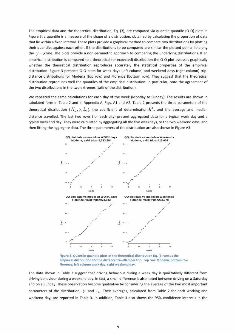
The empirical data and the theoretical distribution, Eq. (3), are compared via quantile-quantile (Q-Q) plots in

Figure 3: a quantile is a measure of the shape of a distribution, obtained by calculating the proportion of data

that lie within a fixed interval. These plots provide a graphical method to compare two distributions by plotting

their quantiles against each other. If the distributions to be compared are similar the plotted points lie along

the y x line. The plots provide a non-parametric approach to comparing the underlying distributions. If an

empirical distribution is compared to a theoretical (or expected) distribution the Q-Q plot assesses graphically

whether the theoretical distribution reproduces accurately the statistical properties of the empirical

distribution. Figure 3 presents Q-Q plots for week days (left column) and weekend days (right column) trip-

distance distributions for Modena (top row) and Florence (bottom row). They suggest that the theoretical

distribution reproduces well the quantiles of the empirical distribution: in particular, note the agreement of

the two distributions in the two extremes (tails of the distribution).

We repeated the same calculations for each day of the week (Monday to Sunday). The results are shown in

tabulated form in Table 2 and in Appendix A, Figs. A1 and A2. Table 2 presents the three parameters of the

theoretical distribution ( 0, ,N L ), the coefficient of determination2R , and the average and median

distance travelled. The last two rows (for each city) present aggregated data for a typical work day and a

typical weekend day. They were calculated by aggregating all the five weekdays, or the two weekend days, and

then fitting the aggregate data. The three parameters of the distribution are also shown in Figure A3.

Figure 3. Quantile-quantile plots of the theoretical distribution Eq. (3) versus the empirical distribution for the distance travelled per trip. Top row Modena, bottom row Florence; left column work day, right weekend day.

The data shown in Table 2 suggest that driving behaviour during a week day is qualitatively different from

driving behaviour during a weekend day. In fact, a small difference is also noted between driving on a Saturday

and on a Sunday. These observation become qualitative by considering the average of the two most important

parameters of the distribution, and 0L . Their averages, calculated from Table 2 for each working and

weekend day, are reported in Table 3. In addition, Table 3 also shows the 95% confidence intervals in the

5 6 7 8 9

56

78

9

QQ plot data vs model on WORK days

Modena, valid trips=1,393,594

Model

Data

5 6 7 8 9

56

78

9

QQ plot data vs model on Weekends

Modena, valid trips=415,004

Model

Data

5 6 7 8 9

56

78

9

QQ plot data vs model on WORK days

Florence, valid trips=973,043

Model

Data

5 6 7 8 9

56

78

9

QQ plot data vs model on Weekends

Florence, valid trips=293,278

Model

Data

10

estimate of the average x , expressed as 1.96 xx SE where /xSE n is the standard error of the

mean with the sample standard deviation and n the number of values. The standard error of the mean is

an estimate of how far the sample mean is likely to be from the population mean.

Table 2. Parameters of the theoretical distribution Eq. (7) per day, per city. Distances in km.

City Week day N 0L 2R

Average distance

Median distance

Modena MON 347,926 0.54 1.89 0.9971 9.33 4.45

TUE 372,904 0.51 1.43 0.996 9.25 4.37

WED 292,181 0.54 1.85 0.9958 9.37 4.44

THU 289,480 0.54 1.86 0.9973 9.44 4.51

FRI 310,286 0.51 1.48 0.9971 9.67 4.51

SAT 269,610 0.49 1.34 0.9961 10.16 4.55

SUN 209,065 0.43 0.9 0.9956 12.53 5.28

WORK days 1,615,498 0.52 1.66 0.9983 9.4 4.45

Weekends 482,025 0.45 1.02 0.9965 11.2 4.84 Florence MON 277,970 0.4 0.42 0.9934 9.55 4.24

TUE 281,195 0.41 0.49 0.9949 9.59 4.31

WED 221,617 0.42 0.59 0.9925 9.71 4.34

THU 227,801 0.41 0.52 0.9924 9.69 4.35

FRI 236,981 0.4 0.43 0.9922 9.98 4.36

SAT 228,675 0.31 0.08 0.9878 10.82 4.43

SUN 179,941 0.28 0.05 0.9889 13.87 5.44

WORK days 1,248,124 0.4 0.47 0.9952 9.69 4.32

Weekends 411,366 0.29 0.05 0.9896 12.21 4.85

The data reported in Table 3 show that driving dynamics during a working and a weekend day are qualitatively

different since the confidence intervals for a week day and a weekend day do not overlap. It is, thus, sufficient

to consider the driving behaviour during a “typical” working and a weekend day, without emphasizing the

behaviour for each single week day (as is frequently done).

Table 3. Average and L0 for work day (WD) and weekend day (WE) with the 95% confidence interval for Modena and Florence.

City Working day or weekend

0 0L L

Modena WD 0.528 ± 0.013 1.702± 0.178

WE 0.460 ± 0.042 1.120 ±0.305

Florence WD 0.408 ± 0.007 0.490 ± 0.055

WE 0.295 ± 0.021 0.065 ± 0.021

3.1.2 Daily mobility distance

An equally important quantity to assess more wide spread public acceptance of electric vehicles is the daily

mobility distance, the total distance (length) travelled in a day. This distance is to be compared to the reported

autonomy of an electric vehicle. The daily mobility distance provides complementary information to the

distance travelled per trip. All trips that start on the same day are accounted for in the calculated total daily

distance (even if they terminate after midnight). Figure 4 presents relative frequencies of the daily mobility

distance for the two cities. As the bin size was chosen to be 1 km, the relative frequencies may be viewed as

11

the corresponding histogram. The cumulative frequency distributions are also shown (in red, specifying the

80th percentile), as well as the average, mean, and mode of the empirical probability density functions. Small

differences between the daily driving behaviour in the two cities are noted. In particular, the average, median,

and mode distances travelled per day are slightly larger in Modena than in Florence: Modena is a smaller city

close to the large city Bologna, so it is likely that some drivers commute to Bologna from Modena.

Figure 4. Relative frequency (bar) and cumulative (red, solid) distributions of daily mobility distance. Left: Modena. Right: Florence.

Note that in both cities 80% of the daily distance travelled by a vehicle is less than 65 km, well within the

reported range of commercially available electric vehicles. Whereas this may suggest that a large part of the

fleet could be easily replaced by electric vehicle (under the assumption that driving behaviour is independent

of the vehicle powertrain), caution should be exercised in interpreting the 80th percentile. It is much more

important to note that 20% of the daily distance travelled is greater than 65 km. If the choice to purchase an

electric vehicle is based only on its reported autonomy, then the buyer may be more interested in the number

of trips he/she would not be able to make than the numerous trips he/she could make. The buyer may place

more weight on the relatively infrequent events, especially if these events are considerably more frequent

than a Gaussian distribution would predict (heavy tails of the non-Gaussian distribution).

The daily mobility data are further analysed in Figure 5. As in the case of the trip-distance distribution, we

modelled the data by an appropriately chosen distribution. We found that a reasonable choice is a power-law

distribution with an exponential cut-off

0

1

( ) exp ,x

y x y xL

(6)

The empirical data and the numerical fit are presented in Figure 5 in a linear-logarithmic plot. The distribution

reproduces very well the GPS-calculated distances for both cities. As before, we fitted the distribution in a

logarithmic scale to ensure that long distances are accurately reproduced. An accurate estimate of the

probability that a vehicle travel a long distance is important as an electric vehicle might not have enough

available energy to complete the trip. In fact, drivers’ anxiety about the autonomy of electric vehicles arises

not from the short-frequent trips, but from the infrequent long trips, which are likely to be driven outside

urban environments.

Daily Mobility Length

(data: Modena)

distance (Km)

Re

lative

fre

qu

en

cy

0 50 100 1500.0

00

0.0

05

0.0

10

0.0

15

0.0

20

0.0

25

Average 40.5

Median 32

Mode 9.5

0.0

0.2

0.4

0.6

0.8

1.0

cu

mu

lative

sca

le

~80% at x=65 km


(data: Florence)

distance (Km)

Re

lative

fre

qu

en

cy

0 50 100 1500.0

00

0.0

05

0.0

10

0.0

15

0.0

20

0.0

25

Average 39.2

Median 29.5

Mode 6.5

0.0

0.2

0.4

0.6

0.8

1.0

cu

mu

lative

sca

le

~80% at x=64 km

12

Figure 5. Daily mobility length distributions: Modena (left), Florence (right).

We remark, as in the previous section, that whereas the functional form of the distribution remains the same,

data from different cities correspond to different parameters. The comparisons suggest that the exponent 𝛼

and the characteristic length 1L depend on the city. City-dependent dynamics, as determined, for example,

from the road and network topology, traffic, population density, points of interest and associated activities,

are reflected in the parameters of the distribution. Since the daily-mobility distance distribution is not

Gaussian, the average distance travelled per day differs significantly from the median (and mode) distance.

Furthermore, the change of the median distance is larger than the change of the average between the cities.

The goodness-of-fit was estimated graphically through the quantile-quantile (Q-Q) plots shown in Figure 6: the

quantile-quantile comparison is reasonably good.

Figure 6. Quantile-quantile plots of the empirical and theoretical, Eq.(6), distributions of the daily distance travelled: Modena (left) and Florence (right).

The model distribution for the single-trip distance and the daily mobility length are compared to theoretically

based distributions proposed in the literature in Figure 7. Bazzani et al. [15] used statistical-physics arguments

to obtain analytical expressions for the single-trip and daily-mobility distance distributions. They suggested

0 50 100 150

2.0

2.5

3.0

3.5

4.0

Daily Mobility Distance

(data: Modena, valid recs=375,739)

distance (Km)

log

10(p

df)

y0 4628L1 34.05

0.28

R2

0.9975

0 50 100 150

2.0

2.5

3.0

3.5

4.0

Daily Mobility Distance

(data: Florence, valid recs=273,781)

distance (Km)

log

10(p

df)

y0 4695L1 38.33

0.14

R2

0.9962

5 6 7 8 9

56

78

9

QQ plot for Daily Mobility Length model

(data: Modena, valid recs=375,739)

Model

Da

ta

5 6 7 8 9

56

78

9

QQ plot for Daily Mobility Length model

(data: Florence, valid recs=273,781)

Model

Da

ta

13

that the single-trip distance distribution may be analytically calculated by determining the distribution of k

uniformly-spread points into a segment of length L : the number of points k is the number of stops a driver

makes, i.e., the number of activities associated with a trip that starts from home and returns home. They

obtained

1

1

( ) ( 1) 1 ,

kNk

N

k

c xp x k ka

L L

(7)

where c is normalization constant and N the maximum number of daily activities. They suggested

0.7, 18a N . The comparison of the single-trip length probability distributions, Eq. (2) for Modena and

Florence and Eq. (7) for Florence (Figure 7, left) is very satisfactory. The data the authors of Ref. [15] used were

floating-car data, obtained from the same company as the data analysed herein, but for a different period

(March 2008). Note, however, that Eq. (7) may become negative for x L , a problem that does not arise for

our proposed distribution, Eq. (2).

Bazzani et al. [15] also suggested that the daily-mobility probability distribution may be expressed as

0

0

( ) exp ,L

p L LL

(8)

where 0L is a characteristic length scale. The normalized to unity probability distribution associated with Eq.

(6) and the function to be compared to Eq. (8) is

1

1 1

( ) exp ,(1 )

x xh x

L L

(9)

where the two parameters are obtained from the fit to the empirical distribution, see, for example, Figure 5.

The comparison of the daily-mobility distributions is not as satisfactory if the characteristic length suggested

by Bazzani et al. [15], 24.9L km, is taken. Instead, better agreement is obtained by increasing the length

scale to 42.5L . Bazanni et al. [15] considered only trips that started within a circle of 10 km around the

historical centre of Florence and remained inside that area: they were interested in selecting drivers who lived

and moved within Florence. Our data, as mentioned, were filtered differently: vehicles which travelled 50% (in

number of trips) outside their respective province were removed. Hence, it might be expected that if the

characteristic length scale in Eq. (8) is increased the agreement would improve, an observation that is

confirmed in Figure 7 (right). Nevertheless, the main difference between the two expressions is the algebraic

growth factor, whose exponent is rather small: its effect is more noticeable at short distances. In fact, our

proposed distribution function Eq. (9) reproduces the short-distance behaviour better than the pure

exponential distribution.

Both works, this work and Ref. [15], suggest that well defined probability distribution functions, with

appropriately chosen parameters, reproduce rather accurately features of driving behaviour, and in particular

the single-trip and daily mobility length probability distributions. Whether the functional form of the

distribution function is universal, and therefore whether it may be derived using generic arguments, via, for

example, arguments based on an appropriately defined entropy or by considering the stochastic behaviour of

drivers, is an issue that shall be addressed in the future. Moreover, further statistical analyses are required to

ensure that the Modena and Firenze distributions are statistically different, i.e., that the two distribution do

not arise from the same distribution within a given confidence.

14

Figure 7. Theoretical probability density function (pdfs, this work) and pdfs obtained via statistical physics arguments, Bazzani et al. [15]. Left: Single-trip length distribution; Right: Daily-mobility distance distribution.

3.1.3 Number of daily trips

The number of daily trips is calculated in the same way as the daily mobility length: it is the total number of

trips that started between the midnights delimiting one day. The number of trips is an important quantity

because it is directly related to the number of daily activities. Figure 8 presents aggregate statistics for Modena

and Florence: in both cases two maxima are noted at 2n . As before, we observe similar behaviour in the

two cities. The distributions of the number of daily trips per week day are presented in Appendix A, Figures A4

and A5. Note that on Sundays the second peak disappears and the remaining unique peak at n=2 becomes

sharper. This is observed for both cities, suggesting, as the previous results imply, that driving behaviour on

Saturdays and Sundays (and the associated activities) is qualitatively different from the behaviour during any

other day. Nevertheless, we suggest that for simplicity and compactness urban mobility may be described by

typical mobility during a working day and a weekend day, even though a stringer analysis would assign

separate driving patterns to a working day, to Saturday, and to Sunday. Thus, three distinct week-day driving

patterns may be identified, which under some conditions may be approximated to only two.

Figure 8. Daily number of trips: Modena (left), Florence (right).

0 5 10 15 20 25 30 35 40-3

-2.5

-2

-1.5

-1

-0.5

Length (km)

log

10(P

robabili

ty d

ensity f

unction)

Single-trip length distribution

Statistical Laws Urban Mobility (Florence), L = 24.9km

Stretched Exponential (Modena), =0.51, L0 = 1.66km

Stretched Exponential (Florence), =0.39, L0 = 0.42km

Daily Number of Trips

(data: Modena)

distance (Km)

Re

lative

fre

qu

en

cy

0 5 10 15 20 25 30

0.0

00

.05

0.1

00

.15

0.2

00

.25

0.3

0

Average 4.6

Median 3.7

Mode 2

0.0

0.2

0.4

0.6

0.8

1.0

cu

mu

lative

sca

le

~80% at n=7


(data: Florence)

distance (Km)

Re

lative

fre

qu

en

cy

0 5 10 15 20 25 30

0.0

00

.05

0.1

00

.15

0.2

00

.25

0.3

0

Average 4.4

Median 3.5

Mode 2

0.0

0.2

0.4

0.6

0.8

1.0

cu

mu

lative

sca

le

~80% at n=6

0 50 100 150-4.5

-4

-3.5

-3

-2.5

-2

-1.5

-1

Length (km)

log

10(P

robabili

ty d

ensity f

unction)

Daily mobility distance distribution

Statistical Laws Urban Mob. (Flor.), =0, L1 = 24.9km

Statistical Laws Urban Mob. (Flor.), =0, L1 = 42.5km

Stretched Exponential (Mod.), = 0.28, L1 = 34.05km

Stretched Exponential (Flor.), = 0.14, L1 = 38.33km

15

3.1.4 Trip starting time and trip duration

The starting time of a trip is the time of the first event of the trip, namely the time the engine is turned on

(MS=1). The distribution of trip-starting times, in terms of relative frequencies, is shown in Figures 9 and 10 for

every week day and each city. The starting time was binned in half-hour bins. During a weekday, we note three

pronounced peaks at approximately 8 h, 13 h, and 18-19 h: the first peak may be associated with a work

activity, the middle with part-time work (possibly) or shopping, and the latter to return from work (office

hours in Italy are usually 8:30-12:30 and 14:30-18:30). Two peaks at approximately 12-13 h and 19-20 h are

noticeable during weekend days (as expected the peaks are slightly shifter to the right as people tend to sleep

longer on weekend mornings).

Figure 9. Distribution of trip starting time per week day and aggregated per working and weekend day (Modena).

Trip duration was calculated from the time of the first event to the time of the last event of a trip. We remind

the reader that two contiguous trips were merged if the vehicle stops for less than 10 minutes. The data were

fitted to the following stretched exponential distribution (normalized to the total number of trips), i.e., the

same functional form as Eq. (3) but with travel time the independent variable

0 0

1( ) exp .

1/

tf t N

T T

(10)

As before, see discussion of the trip-distance distribution, we used non-linear regression on the logarithmic

scale to obtain the three parameters of the distribution. The normalization condition ensures that the total

number of trips N is reproduced. The results are shown in Figure 11, along with the model parameters and

basic statistical quantities expressed in fractions of an hour.

0 5 10 15 20

0.0

00.0

6

Day: MON

trips: 312,714

Time of the day (h)

Rela

tive fre

q.

0 5 10 15 20

0.0

00.0

6

Day: TUE

trips: 320,028

Time of the day (h)

Rela

tive fre

q.

0 5 10 15 20

0.0

00.0

6

Day: WED

trips: 258,378

Time of the day (h)

Rela

tive fre

q.

0 5 10 15 20

0.0

00.0

6

Day: THU

trips: 260,228

Time of the day (h)

Rela

tive fre

q.

0 5 10 15 20

0.0

00.0

6

Day: FRI

trips: 270,971

Time of the day (h)

Rela

tive fre

q.

0 5 10 15 20

0.0

00.0

6

Day: SAT

trips: 231,915

Time of the day (h)

Rela

tive fre

q.

0 5 10 15 20

0.0

00.0

6

Day: SUN

trips: 184,433

Time of the day (h)

Rela

tive fre

q.

0 5 10 15 20

0.0

00.0

6

Day: Work days

trips: 1,422,319

Time of the day (h)

Rela

tive fre

q.

0 5 10 15 20

0.0

00.0

6

Day: Weekends

trips: 416,348

Time of the day (h)

Rela

tive fre

q.

16

Figure 10. Distribution of trip starting time per week day and aggregated per working and weekend day (Florence).

A similar analysis was performed for each day of the week and aggregated per working day and weekend day.

The results are shown in Appendix A, Figures A6 and A7. Different driving behaviour during a weekday and a

weekend may be noted. In fact, as mentioned earlier, driving behaviour during the two weekend days seems

qualitatively different, whereas driving behaviour during a (working) weekday appears rather similar.

Figure 11. Trip-duration distributions, and their parameters, Eq. (18), for Modena (left) and Florence (right).

0 5 10 15 20

0.0

00.0

6

Day: MON

trips: 220,880

Time of the day (h)

Rela

tive fre

q.

0 5 10 15 20

0.0

00.0

6

Day: TUE

trips: 222,652

Time of the day (h)

Rela

tive fre

q.

0 5 10 15 20

0.0

00.0

6

Day: WED

trips: 180,019

Time of the day (h)

Rela

tive fre

q.

0 5 10 15 20

0.0

00.0

6

Day: THU

trips: 182,741

Time of the day (h)

Rela

tive fre

q.

0 5 10 15 20

0.0

00.0

6

Day: FRI

trips: 188,364

Time of the day (h)

Rela

tive fre

q.

0 5 10 15 20

0.0

00.0

6

Day: SAT

trips: 160,108

Time of the day (h)

Rela

tive fre

q.

0 5 10 15 20

0.0

00.0

6

Day: SUN

trips: 134,960

Time of the day (h)

Rela

tive fre

q.

0 5 10 15 20

0.0

00.0

6

Day: Work days

trips: 994,656

Time of the day (h)

Rela

tive fre

q.

0 5 10 15 20

0.0

00.0

6

Day: Weekends

trips: 295,068

Time of the day (h)R

ela

tive fre

q.

0 1 2 3 4 5 6

12

34

56

Trip Duration

(data: Modena, valid trips=1,816,512)

time (h)

log

10 o

f co

un

ts

T0 0.01710.44

N 2538218

R2

0.9945

Average 0.27

Median 0.21Mode 0.12

0 1 2 3 4 5 6

12

34

56

Trip Duration

(data: Florence, valid trips=1,271,067)

time (h)

log

10 o

f co

un

ts

T0 0.01770.43

N 1886019

R2

0.9953

Average 0.31


17

3.1.5 Work trips

Work trips are defined as trips that consist of two legs, the origin of the first leg being the destination of the

second and vice versa, with a time difference between the two legs of 7.5 to 9 hours (typical duration of a

working day). The identification of such trips, and their duration, is important in determining drivers’ activities

and origin/destination matrices. Trips defined as described are not necessarily trips to a working location as

they could correspond to any other regularly performed activity, irrespective of whether it is remunerated or

not. Origin destination locations were determined with a tolerance of 500 meters, computed from the

(longitude, latitude) GPS coordinates as a straight line (Euclidean distance) between the start of the first leg

and end of the returning leg.

Trip distance

The corresponding trip-distance distributions were fitted to a generic stretched exponential distribution, see,

for example, Eq. (3). Results are shown in Figure 12. If these results are compared to the distribution of all the

trips during a working day, Figure 2, we note that the average (and median) distance travelled increases to

12.6 km from 9.4 km (Modena) and to 13.1 km from 9.8 km (Florence). A trip to work tends to be longer than

an average trip.

Similarly, we analysed the behaviour of these trips for each week day, reported in the Annex, Figures A8 and

A9. The details of the distance distributions are shown there. We find that, as expected, there are considerably

fewer trips during the weekend that may be characterized as work trips. The proportion of weekend generic

work trips to week day work trips is approximately 25%, whereas the proportion of either week day or

weekend trips to the total number of trips is approximately 3.5% (irrespective of city).

Figure 12. Observed and modelled, Eq. (3) distribution of work-trip distances: Modena (left), Florence (right).

Travel time

We calculated and modelled the travel time distributions for work trips. The data were fitted to a stretched

exponential distribution of the form reported in Eq. (10), normalized to the total number of work trips. We

decided to neglect the first reported point that represents counts between 0 and 5 min, and to neglect all trips

that lasted longer than 3h: their number was deemed too low to fit. The results are shown in Figure 13. We

note that the average work-trip duration is slightly longer than the average duration of all trips: surprisingly,

the median, however, is slightly lower. We also generated the distributions per week day, and aggregated on

working day and weekend: these calculations are presented in Appendix A, Figures A10 and A11.

0 20 40 60 80 100

01

23

4

Work-trip Distance

(data: Modena, Valid trips=78,739)

distance (Km)

log

10 o

f co

un

ts

L0 5.420.69

N 80674

R2

0.9841

Average 12.6

Median 8.5Mode 1.5

0 20 40 60 80 100

01

23

4

Work-trip Distance

(data: Florence, Valid trips=54,741)

distance (Km)

log

10 o

f co

un

ts

L0 3.010.56

N 57735

R2

0.9706

Average 13.1

Median 7.5Mode 1.5

18

Figure 13. Distribution trip duration of work trips with fitted model parameters, Eq. (10): Modena (left), Florence (right).

3.1.6 Average trip speed, motion speed, and segment speed

The average trip speed is calculated as the total distance travelled per trip divided by the total trip time (note

that the maximum intermediate stop time is 10 minutes). The average motion speed, defined as the total

distance divided by the time the vehicle is moving, i.e., excluding stopping times, was also calculated. The

segment speed is the speed between two GPS events obtained by dividing the distance travelled, as given in

the data, by the time between the two events. Figure A12, Appendix A, presents the distributions of the

average speed, the average motion speed and the segment speed for Modena and Florence. The distributions

per week (and weekend) day do not present particular differences between the various days; they are not

included in this document.

The data on average motion speed were fitted to two Gaussians and an exponential. We stress that the

purpose of the fit is not to suggest a general functional form, as in the fits of the previous experimental

distributions, but to capture their salient features. In particular, two Gaussians were chosen to identify the two

peaks shown in Figure 14 (left Modena, right Florence). The chosen functional form is

2 2

1 2

0

v(v) exp exp v v exp v v ,

vf A B C D B

(11)

where 1v and 2v are the positions of the two relative maxima. These maxima can be found by a simple

algorithm, but we had to adjust the first peak (Modena) by an offset (2 km/h) to improve the fit. The values

are 1v =15.5 km/h and 2v =37.5 km/h for Modena and 1v =9.5 km/h and 2v =39.5 km/h for Florence. Also

note that the exponent is less than unity, therefore the first term is a stretched exponential function.

We suspect that city topology plays a role in determining the shape of these distributions. In particular, the

second visible peak for the city of Modena (Figure 14, left) could be attributed to commuting (Modena is close

to the much larger city of Bologna), or, in any case, to the use of a high-speed highway. This peak is absent in

the Florence data as Florence is a commuting hub, and city drivers do not commute to a larger city nor do they

use on average a high speed highway during their daily routine.

0 1 2 3 4 5

01

23

45

Work-trip Duration

(data: Modena, valid trips=79,205)

time (h)

log

10 o

f co

un

ts

T0 0.05570.55

N 100305

R2

0.99

Average 0.3


0 1 2 3 4 5

01

23

45

Work-trip Duration

(data: Florence, valid trips=54,978)

time (h)

log

10 o

f co

un

ts

T0 0.10680.64

N 66127

R2

0.99

Average 0.34

Median 0.2Mode 0.12

19

Figure 14. Average motion speed and its fit (red line), with calculated segment speed (triangles) for Modena (left) and Florence (right).

3.1.7 Parking

The vehicle parking (stopping) time and location are of great importance in the context of electro-mobility as

they represent potential opportunities for recharging. For example, their geographical distribution may be

analysed to suggest possible locations of future charging stations. In the Floating-car data parking times are

obtained from the time difference between an engine off event (code MS=2) and the next engine on event

(code MS=0). Figure 15 shows day and night parking spots for the city of Modena. It may be surmised that

overnight parking is to be associated with private night parking.

Figure 15. Day (left) and night (right) parking time distribution in the city of Modena.

We also analysed the distribution of the duration of parking times. Non-linear regression was performed with

a stretched exponential and four Gaussians centred at relative maxima. Regression of the stopping/parking

times then follows the model

4

2

1

ln( ) exp ,i i i

i

y Ax G g x x C

(12)

where , , , ,i iA G g C are parameters to be determined by the non-linear regression, while xi (for i=1,..,4)

are the positions of the Gaussian peaks, determined as the relative maxima in an interval around the peak.

Only the first bin (zero to 6 min stop time) is excluded by the regression. The results are shown in Figure 16.

As in the case of the average motion, the only valuable information to be obtained from the generic fit of Eq.

(12) is the identification of the relative maxima (and their possible interpretation). In particular, we note that

the first peak is in exactly the same position for both cities, while the others differ by little (each decimal point

0 20 40 60 80 100

0.0

00

0.0

05

0.0

10

0.0

15

0.0

20

0.0

25

0.0

30

Average Speed (circles) and Segment Speed (triangles)

(valid trips: 1,816,612 - valid segments: 14,619,571)

Speed (km/h)

Re

lative

Fre

qu

en

cy

0 20 40 60 80 100

0.0

00

0.0

05

0.0

10

0.0

15

0.0

20

0.0

25

0.0

30

A 0.006513947

T0 0.0184689

0.00315165

B 15.32673

C 2.21799

D 0.0227667

E 0.006513947

R2

0.9895773

Average 30.2

Median 28.5

Mode 19.5

0 20 40 60 80 100

0.0

00

0.0

05

0.0

10

0.0

15

0.0

20

0.0

25

0.0

30

Average Speed (circles) and Segment Speed (triangles)

(valid trips: 1,271,204 - valid segments: 30,871,306)

Speed (km/h)

Re

lative

Fre

qu

en

cy

0 20 40 60 80 100

0.0

00

0.0

05

0.0

10

0.0

15

0.0

20

0.0

25

0.0

30

A 0.001144358

T0 0.0007005688

0.0002424379

B 12.06904

C 2.318561

D 0.03676629

E 0.001144358

R2

0.9906095

Average 27.3

Median 24.5

Mode 18.5

20

corresponds to 6 minutes, so 3 0.2x corresponds to a 12-minute difference). A possible interpretation of

these distributions is that the first peak is due to the part time jobs or other daily activities (shopping) at

approximately 4 hours, the second (approximately at 9 hours) to standard-hour jobs, while the third (at 12

hours) and the fourth (at 19 hours) to night stops. The distributions were plotted in a logarithmic scale to

render the four peaks visible.

Figure 16. Parking time duration for Modena (left) and Florence (right), with the regression model and centres of the four Gaussians.

3.1.8 Discussion

We conclude this Section by mentioning previous attempts to unravel, understand, and possibly simulate

individual human mobility patterns. The studies reported in Refs. [16-19] analysed large-scale human mobility

patterns obtained from tracking dollar bills (via online bill-tracking websites which monitor the world-wide

dispersal of large numbers of individual bank notes [16]) or from tracking anonymized mobile phone users

[17,18,19]. The mobility patterns were considered to be described by three indicators: the trip distance

distribution, the radius of gyration (to be defined in the next paragraph), and the number of visited locations.

They suggested that long-distance human displacements may be described (on average) by the truncated

power law

( ) exp .r

p r r

(13)

The power-law exponent is believed to be, for different datasets, 1.75 0.15 (mean plus/minus

standard deviation) and the cut-off values 400 or 80 km, depending on the data analysed. Note that

the length scale of the cut-off exponential is of the order of 100 kilometres, a distance considerably larger than

the distances analysed in this report. The interesting feature of the power-law distribution Eq. (13) is that it is

scale-invariant, namely it does not have a characteristic length scale associated with the observed mobility

patters. The length scale associated with the exponential function is only relevant for very large distances, an

effect known as “finite-size” effect in condensed matter physics. The absence of a characteristic scale implies

some kind of universality, namely features of the distribution do not depend explicitly on the nature of small-

21

scale, local interactions. As such, the authors proposed plausible universal mechanism that would lead to a

truncated power-law probability distribution, such as a continuous random walk process.

In our analyses, we did not considered the so-called radius of gyration, a concept borrowed from polymer

physics that describes the mass distribution about a polymer’s centre of mass. In its application to the study of

human mobility, an individual’s radius of gyration can be interpreted as the characteristic distance an

individual travels within a time interval. The distribution of the radius of gyration revealed considerable

heterogeneity, that is most individuals travel within a short radius, but others cover long distances on a regular

basis [19]. This observation is implicit in the heavy tails of the theoretical distributions used to model trip

distance and the daily mobility distance.

22

3.2 Survey data The Survey data were collected in six European countries; the aim of the survey was to gather information

about conventional-vehicle usage under conditions for which national surveys had not previously provided

sufficient information. The Survey data were extensively analysed in Refs. [10-12]. Table 4 provides a summary

of the main features of the data as determined by the Java processing software.

Table 4. Survey data summary.

Total number of distinct vehicles (with at least one trip) 3,489

Number of excluded vehicles 0

Regular Trips 39,955

Anomalous Trips 5

Regular Stops 39,959

Percentage of anomalous trips (with full trip removal) 0.01%

Anomalous Stops 0

Contiguous Trips found (stop<10.0 min) 833

Work Trips found 0

Records read 122,379

Computational time (s) 1.72

We, also, analysed these data with the methodology used to analyse the Floating-car data for Modena and

Florence. We do not report the results of our analysis since the quality of the data is not comparable to the

quality of the Floating-car data, in that there are considerably fewer data. Moreover, the analysis does not

suggest any significant new features. It is perhaps worth mentioning that we noted a consistent bias in the

data. It appears that reported values of distances travelled tended to be multiples of 5 or 10 kilometres. Such

multiples appeared roughly 3 or 4 times more frequently than intermediate values, a possible result of the

data acquisition through trip diaries. The analysis of the Survey data will focus on their comparison with the

other datasets to check their compatibility with the theoretical distributions presented in the previous

subsection. This analysis is presented in Section 5.

23

4. Electric vehicles: Green eMotion project

The data collected during the Green eMotion project (GeM) [5] provide a significant database of electric-

vehicle usage. Data were collected from March 2011 to Dec. 2013 in six Demonstration Regions. The database

comprises about 165,000 events (including recharging events): it represents one of the largest and more

detailed databases of real-world data for electric vehicles in Europe. We identified a total of 457 electric

vehicles for which sufficient information was available in the database: for example, apart from the

information required for a conventional vehicle (as analysed previously) the powertrain technology is an

important additional variable. The distribution of vehicles types and powertrain technologies is given in Table

5. In our analyses we used only the 357 battery electric cars for which trip information (distance and duration)

was available. We refer to these cars as BEV in the following.

Table 5. Distribution of vehicles per type and technology (GeM).

Technology cars motorcycles transporter

BEV 357 11 33

PHEV 56 0 0

Table 6 presents the number of trips whose length is non-zero, as well as those for which information on the

energy consumed is available, parameterized by vehicle make and model. We note that the two cars with the

largest number of trips are the Mitsubishi i-MiEV and the Peugeot iOn. Trips driven by these two cars

constitute 85% of all trips for which the necessary information was available. These two cars are very similar:

the iOn (and also the C-Zero) is the i-MiEV slightly modified for the Peugeot/Citroen brands. Both vehicles

belong to segment A and they are considered “small-sized” cars. Reported technical specifications for the 2015

i-MiEV are: length 3.475 mm, width 1,475 mm, height 1,610 mm; curb weight 1085 Kg; electric motor 47 KWh,

Li-ion battery of 16 kWh, range (NEDC) 160 km, electric energy consumption (NEDC) 125 Wh/km (135 Wh/km

for the 2012 version), charging time approximately 8 h (regular) and approximately 30 min (80% of full charge,

fast charger) [20]. Hence, the 357 BEV cars analyzed in this Section may be considered to be small variants of

the Mitsubishi i-MiEVs.

Table 6. Vehicle make and model with the number of non-zero length trips and energy consumption.

Vehicle Make-Model Type Number of trips of non-

zero length Number of trips of non-zero length and

with valid energy consumption data

no make-no model available car 533 305

Citroen C-Zero car 141 137

Mitsubishi i-MiEV car 31,428 19,594

Peugeot iOn car 25,453 24,080

THINK City car 8,244 7,911

We analysed the Green eMotion data following the approach used to analyse the Floating-car data with minor

modifications to incorporate battery charging and energy usage (battery discharge). To process the data with

the same software the electric-vehicle data were pre-processed to transform them to an adequate form. The

changes ensured that the correct event types were identified (by the appropriate parsers). Specifically, a

charging event was classified as anomalous if the energy recharged was less or equal zero, if its duration was

zero, and if the distance between the locations of the beginning of charging and its end was greater than 30

meters (Euclidean distance, if GPS coordinates are available). For every trip, which is represented as a single

line in the original set, we created 3 associated events: one with an engine start index (MS=0), one in motion

containing the distance travelled (MS=1), and one with an engine off (MS=2) corresponding to the end of the

trip. As in our analyses of conventional vehicles, we joined two consecutive trips to a contiguous trip if the

24

stopping time between the two events was less than 10 min. For the charging events, we introduced new

event codes, MS=100, 101, 102, indicating the start, charging, and end of charge (respectively). Thus, a charge

event, which is a single line in the Green eMotion dataset, is transformed into 3 lines, each one with a time

stamp, a code, and a number that may be interpreted by the previously described software.

4.1 Mobility characteristics Figure 17 (left) presents the trip-distance distribution as a histogram, binned in 3 km bins, for the 357 BEVs

(cars). We found that a 3 km binning provides a reasonable representation of the empirical distribution. The

red line shows the cumulative trip distribution: it shows that 80% of the trips travelled a distance less than 10

km. The right subfigure shows the distribution of the duration of the trips, binned at 10 minutes. A

predominance of short trips is noted: 80% of the trips lasted less than 22.2 min, the median trip duration was

0.06 hours (3.6 min), and the average trip duration 0.21 hours (12.6 min). For a comparison with conventional-

vehicle mobility see Table 7.

Figure 17. Left: trip distance distribution (bars) with cumulative distribution. Right: trip duration.

As in the case of the Floating-car data, the distance travelled per trip and per day of the week is of particular

interest, as such distributions provide indications on different activities performed during the day. We present

the data, along with average, median and mode of the corresponding distributions, in Appendix A, Figure A13.

One of the most important quantities to assess the viability of electric vehicles is the daily mobility distance,

the total distance (length) travelled in a day. The daily mobility distance provides information complementary

to the distance travelled per trip. This distance is to be compared to the reported autonomy of an electric

vehicle. All trips initiating on the same day are accounted for in the calculated total daily distance (even if they

terminate after midnight). Figure 18 presents the distribution of the daily mobility length (the sum of the

length of all trips initiated on the same day), and its cumulative distribution (left), whereas the daily number of

trips is shown in the right subfigure.

Trip Distance

(valid trips=65,799)

distance (Km)

Re

lative

fre

qu

en

cy

0 10 20 30 40 50 60

0.0

0.1

0.2

0.3

0.4

Average 6.2

Median 1.9

Mode 4.5

0.0

0.2

0.4

0.6

0.8

1.0

cu

mu

lative

sca

le

~80% at d=10 km

Trip Duration

time (h)

Re

lative

fre

qu

en

cy

0.0 0.5 1.0 1.5 2.0 2.5 3.0

0.0

0.1

0.2

0.3

0.4

0.5

Average 0.21

Median 0.06

Mode 0.08

0.0

0.2

0.4

0.6

0.8

1.0

cu

mu

lative

sca

le

80% at t 22.2 min

25

Figure 18. Left: Daily mobility distance relative frequency (bar) and cumulative (red, solid) distributions. Right: Relative frequency (bar) and cumulative distribution (red, solid) of daily number of trips.

The daily mobility distance is further compared to the daily distance covered by conventional vehicles by

fitting the probability distribution function to the power-law distribution with an exponential cut off, Eq. (6).

The results are shown in Figure 19. The fitting parameters were obtained using a distance range from 3 to

140km. The fit reproduces rather accurately the data, providing further support that the chosen distribution

describes well the daily-mobility distance. As previously argued, specific features of the city or drivers’

behaviour are reflected in the choice of the distribution parameters. The daily mobility distribution and the

corresponding fit per day of the week are show in the Appendix, Figure A14.

Figure 19. Daily mobility distance: data (points), fit (solid, red line); Left: linear scale. Right: logarithmic scale.

Table 7 compares aggregate statistical quantities for a number of mobility variables associated with

conventional mobility (Floating- car data) and electro-mobility (GeM). The Survey data are not included. We

note that the most frequently used statistical quantities (average, mean, and mean) of the trip distance, trip

duration, and daily mobility distance are lower for the cars that participated in the Green eMotion than for the

Floating-car vehicles. The same conclusion may be drawn by comparing the characteristic length scale 1L of

the daily-mobility distribution: it is approximately 34-38 km for the floating-car database and 24 km for the

Green eMotion database. It seems that drivers of electric vehicles drive for a shorter time and fewer


distance (Km)

Re

lative

fre

qu

en

cy

0 50 100 150

0.0

00

.02

0.0

40

.06

0.0

80

.10

Average 32.5 Km

Median 25.4 Km

Mode 13.5 Km

0.0

0.2

0.4

0.6

0.8

1.0

cu

mu

lative

sca

le

~80% at x=51 km


distance (Km)

Re

lative

fre

qu

en

cy

0 5 10 15 20 25 30

0.0

00

.05

0.1

00

.15

0.2

00

.25

0.3

0

Average 4.6

Median 2.9

Mode 2

0.0

0.2

0.4

0.6

0.8

1.0

cu

mu

lative

sca

le

~80% at n=7

0 50 100 150

0.0

00

.01

0.0

20

.03

0.0

40

.05

0.0

60

.07


(valid recs=14,253)

distance (Km)

Re

lative

fre

qu

en

cy

y0 184.1

L0 24.2

0.39

R2

0.9771

0 50 100 150

0.0

0.5

1.0

1.5

2.0

2.5

3.0

3.5


(valid recs=14,253)

distance (Km)

log

10 o

f co

un

ts

y0 184.1

L0 24.2

0.39

R2

0.9771

26

kilometres per trip and per day than drivers of vehicles with internal combustion engines. This could also be a

result of the car-size segment as well as the urban driving bias that dominates the GeM sample, whereas the

Floating-car data covers more segments and a higher share of extra-urban driving. The same quantities for the

number of trips per day are rather similar.

Table 7. Descriptive statistics of mobility variables: conventional versus electric vehicles.

Average Median Mode

Trip distance (km) Floating-car, Modena 9.4 (wd

2),11.2 (we

3) 4.5 (wd), 4.8 (we) 1.5

Floating-car, Florence 9.7 (wd),12.2 (we) 4.3(wd), 4.9 (we) 1.5 GeM 6.2 1.9 4.5

Trip duration (min) Floating-car, Modena 15.6 12 7.2 Floating-car, Florence 17.4 12 7.2 GeM 12.6 3.6 4.8

Trips per day Floating-car, Modena 4.6 3.7 2.0 Floating-car, Florence 4.4 3.5 2.0 GeM 4.6 2.9 2.0

Daily mobility distance (km) Floating-car, Modena 40.5 32.0 9.5 Floating-car, Florence 39.2 29.5 6.5 GeM 32.5 25.4 13.5

The following figures summarize aspects of the driving behaviour of electric-vehicle drivers. Figure 20 presents

the relative frequencies of trip starting times, the time of the day a trip starts, and the relative frequencies of

parking times, the time a trip ends. Times are binned in 1h bins.

Figure 20. Trip start (left) and stop (right) time distributions as a function time of the day.

Figure 21 presents the percentage of circulating vehicles, binned per hour.

2 Weekday.

3 Weekend.

Trip Start Time

time of the day (h)

Re

lative

fre

qu

en

cy

0 5 10 15 20

0.0

00

.02

0.0

40

.06

0.0

80

.10

Average 13.5

Median 13.2

Mode 16.5

Trip Stop Time

time of the day (h)

Re

lative

fre

qu

en

cy

0 5 10 15 20

0.0

00

.02

0.0

40

.06

0.0

80

.10

Average 13.7

Median 13.4

Mode 16.5

27

Figure 21. Percent of circulating cars during the day.

Figure 22 shows the relative frequency of the time parking starts and its duration.

Figure 22. Beginning of parking (stop) during the day (LEFT), and parking (stop) duration, including charging times (right). Cumulative frequencies in red.

Figure 23 presents the relative frequencies of charge starting time and the percent of cars plugged to a charger

during the day.

Percent of circulating vehicles

time of day (h)

%

02

46

81

0

0 5 10 15 20

Average 13.3

Median 13.1

Mode 16.5

Beginning of Parking

time of day (h)

Re

lative

fre

qu

en

cy

0 5 10 15 20

0.0

00

.02

0.0

40

.06

0.0

80

.10

Average 13.7

Median 13.4

Mode 16.5

Parking Time Duration

(valid stops=60,977)

duration (h)

Re

lative

fre

qu

en

cy

0 5 10 15 20

0.0

0.1

0.2

0.3

0.4

0.5

Average 3.32

Median 0.11

Mode 0.5

0.0

0.2

0.4

0.6

0.8

1.0

cu

mu

lative

sca

le

28

Figure 23. Charge start time distribution (left) and percentage of cars plugged-in at every hour (computed from the charge starting time and its duration), right.

Lastly, Figure 24 presents the number of charges per day along with the energy recharged, namely the amount

of energy recharged in the battery, binned at 1 kWh. Note that the percentage of circulating vehicles (Figure

21) closely resembles the starting/stopping trip time distribution (Figure 20) and the beginning of parking

distribution (Figure 22), suggesting that the duration of trips is relatively short.

Figure 24. Number of charges during a day (left) and recharge amounts distribution (quantity of energy recharged) (right). Cumulative frequencies in red (solid lines).

4.2 Energy consumption and charging Figure 25 presents the average energy charged per unit time (power) during the day, binned in hours. The

power requested is presented in two modes: on the left, it is normalized to the number of charges performed

during that hour, and, on the right, in absolute terms (not normalized) for all countries.

Charge Start Time

time of day (h)

Re

lative

fre

qu

en

cy

0.0

00

.02

0.0

40

.06

0.0

80

.10

0 5 10 15 20

Average 14

Median 13.7

Mode 8.5

Percent of cars plugged-in

time of day (h)

%

02

46

81

0

0 5 10 15 20

Average 12.2

Median 12.5

Mode 21.5

Number Of Charges Per Day

number of charges

Re

lative

fre

qu

en

cy

0.0

0.2

0.4

0.6

0.8

1 2 3 4 5 6 7 8 9

Average 1.42 charges/day

0.0

0.2

0.4

0.6

0.8

1.0

cu

mu

lative

sca

le

Energy Recharged

(valid charges=72,819)

energy (KWh)

Re

lative

fre

qu

en

cy

0.0

00

.02

0.0

40

.06

0.0

80

.10

0.1

20

.14

0 5 10 15 20 25

Average 6.12 KWh

Median 4.08 KWh

Mode 3.5 KWh

0.0

0.2

0.4

0.6

0.8

1.0

cu

mu

lative

sca

le

29

Figure 25. Energy charged during the day per charge (left), the total amount over all countries (right).

We also analysed the State-of-Charge (SoC) of the vehicle battery by considering it at the beginning and at the

end of a charging operation. The relative frequencies are shown in Figure 26: in the left subfigure the battery

SoC at the beginning of charging is shown, whereas the right subfigure presents it at the end of charging. The

state of charge is considered as a percentage of battery charge with respect to the maximum battery capacity.

Recall that the absolute value of energy recharged is shown in Figure 24 (right). The power-per-charge data

show a minimum early in the morning (approximately at 06:00) and a peak at midday, decreasing slightly

afterwards. The total power requested also shows a minimum early in the morning, but it remains flat for most

of the day (from 10:00 to 23:00). This figure should be contrasted to Fig. 22 (left) where the time parking

begins is plotted. The difference in the overall shape of the relative frequencies between power requested and

beginning of parking suggests that the electric vehicles used controlled charging, and that the time parking

starts does not provide sufficient information to deduce power (or energy) requested from the grid.

Figure 26. State of charge of the battery at the beginning and at the end of charging.

Inspection of Figure 26 shows that, contrary to what one would have expected, users tend to charge their

vehicles at every opportunity they have, and not only when the state of charge is low: the relative frequencies

of the SoC at the beginning of a recharge operation peak at about 70-80% charge . This is referred to as

opportunity charging. The desire to charge irrespective of the state-of-charge of the battery is further

confirmed by noting that more than 40% of charging operations end with a full battery, as shown in the right

Power requested per charge

time of day (h)

po

we

r (K

W)

0.0

0.5

1.0

1.5

2.0

2.5

3.0

0 5 10 15 20

Average 1.45 KW

Total power requested

time of day (h)

po

we

r (M

W)

01

02

03

04

0

0 5 10 15 20

Average 20 MW

State of Charge at Start of Charging

(recs: 25607)

Percent of charge (%)

Re

lative

fre

qu

en

cy

0.0

00

.02

0.0

40

.06

0.0

80

.10

0.1

20

.14

0 10 20 30 40 50 60 70 80 90 100

Average 61.61

Median 65.06

Mode 72.5

0.0

0.2

0.4

0.6

0.8

1.0

cu

mu

lative

sca

le

State of Charge at End of Charging


Re

lative

fre

qu

en

cy

0.0

0.1

0.2

0.3

0.4

0.5

0 10 20 30 40 50 60 70 80 90 100

Average 79.67

Median 85.72

Mode 97.5

30

graph of Figure 26. We think that the predominance of opportunity charging should be viewed with caution.

The behaviour of drivers of electric vehicles may vary with time of usage: frequent charges may be more

common initially and could become less frequent as the driver appreciates battery capacity and the vehicle’s

autonomy.

Figure 27, left, shows the percent energy variation, namely the change of battery SoC per charge, a relative

measure of energy recharged. We also computed the total distance travelled between two charging

operations, Figure 27, right. Its relative frequency appears to be compatible with the daily mobility length, see

Figure 18, left: the 80th percentile at 45 km shows a surprising similarity to the corresponding value of the

daily mobility length, 51 km. This suggests that, on average, a vehicle is charged only once per day, in

agreement with Figure 24.

Figure 27. Percent variation of energy charged (left), total distance travelled between consecutive charges (right).

The relationship between energy charged and time to charge the battery may be parametrized by the type of

vehicle, its technology, battery type, or its use. Since PHEV and BEV employ qualitatively different technologies

(in the sense of a driver’s strategy to recharge) a comparison between these two technologies would have

provided further insights into drivers’ behaviour. Unfortunately, the only available data refer to BEV vehicles.

Figure 28 shows the energy recharged as a function of recharge time parametrized by vehicle type (car,

transporter, moto) and use (private or business use, renting, captive fleet). The points at the far left indicate

fast charging events. Note that the points in the graph don’t necessarily indicate real time charging, but the

duration of the connection to the grid and the energy drawn from the grid during that period. This explains the

points at the lower right end of the graphs. These events, as well as a large part of the slow charging events,

can be considered as suitable for controlled charging, and hence load shifting in the electricity grid.

As BEV cars constitute an important portion of BEV vehicles, we present the same analysis only for them in

Figure 29: this figure is an expanded version of the left subfigure of Figure 28. Data are presented in terms of

fleet type in the four subfigures: private use, business use, rental, captive fleet.

Of particular interest of the recharge energy dataset is the information it provides on energy consumption per

distance travelled, since it can be used to determine real-life vehicle autonomy. The energy consumption per

kilometre is used in numerous computer codes, e.g. COPERT [21], to study fuel consumption and emissions. As

argued, we have to distinguish powertrain technologies since the electric energy consumed by plug-in hybrid

vehicles depends on the mix of electric-thermal energy used, and not solely on the driving pattern and the

distance covered, as is the case for purely electric vehicles. Herein, we analyse only BEV cars.

Energy Recharged


Re

lative

fre

qu

en

cy

0.0

00

.02

0.0

40

.06

0.0

80

.10

0.1

20

.14

0 10 20 30 40 50 60 70 80 90 100

Average 23%

Median 18.1%

Mode 7.5%

Distance Travelled between Charges

(aggregate trips=13,779)

distance (Km)

Re

lative

fre

qu

en

cy

0 50 100 150 2000.0

00

0.0

10

0.0

20

0.0

30

Average 29.5

Median 21.9

Mode 10.5

0.0

0.2

0.4

0.6

0.8

1.0

cu

mu

lative

sca

le

~80%at d=44.6 km

31

Figure 28. Recharged energy as a function of recharge time (BEV vehicles), subdivided per vehicle type. Left: cars, excluding cars with unknown usage type; Right: transporters (red) and motorcycles (green).

Figure 29. Recharge time versus energy recharged, BEV cars, subdivided by usage.

Figure 30 presents the energy consumed per distance in a scatter plot. The symbols denote car usage, the

colour code average trip speed. We performed a linear fit to obtain an approximate indication of consumption

trends. We considered only trips of length up to 50 km, which represent 99.15% of all the data, because the

scatter was considerable for longer trips and their number relatively low. The linear-fit model yields (see, also

the legend of Figure 30) for the energy consumed E (in Wh)

182 0.3 ,E d (14)

where the brackets denote an average and d is the distance in kilometres. The error estimate of the slope is

the standard error. We note that the spread of the data about the linear fit increases asymmetrically (with

respect to the linear model) as the speed increases. This asymmetric feature may be captured by a fit of the

32

positive and negative residuals (the two yellow lines). Figure 31 shows the energy consumed versus trip

distance for vehicles classified according to fleet type or use.

Figure 30. Energy consumption versus trip distance. The colour code denotes average trip speed (km/h).

Figure 31. Energy consumption per distance subdivided by car usage, colour code as in Figure 30.

An alternative way to look at the energy consumption is the distribution of the energy consumed per unit

length of trip, E/d. The corresponding relative frequencies are shown in Figure 32.

33

In agreement with Ref. [5], trips that consumed more than 1000 Wh/km were discarded, as such consumption

was deemed highly unlikely. Thus, the average energy consumed per kilometre may be calculated from the

relative frequency histogram via the appropriate weighted average

1

208 104 Wh/km.N

ii

i i

EEn

d d

(15)

where in is the number of trips in bin i , the total number of bins being N , and id the distance that

corresponds to bin. The variation here represents the standard deviation. We note that there is an

approximate 14% difference between the slope predicted by the linear model, 182 Wh/km, Eq. (14), and that

predicted by the average of the E/d distribution, 208 Wh/km, Eq. (15). This difference is attributed to the two

different averaging procedures. In particular, the result shown in Eq. (15) is a ratio estimator, i.e., it is related

to the ratio of the means of two variables. It is known that such estimators are biased. We thus consider the

result of Eq. (15) less representative of real-life consumption than the prediction of Eq. (14).

Figure 32. Relative frequencies of energy consumed by BEVs per trip length.

More importantly, inspection of the distribution, Figure 32, manifests that it is not a Gaussian distribution.

Hence, a more robust estimate of the energy consumed per kilometre is provided by the median instead of the

average. Equivalently, the most reliable estimator for E/d is the median of the distribution since ratio

estimators are better described by the median of the corresponding relative frequency histograms. For the

truncated distribution, energy per kilometre within 0 to 1000 Wh/km, shown in Figure 32 we found that the

median is186 55 Wh/km , where the spread about the median is the median absolute derivation (a

generalization of the standard deviation for robust statistical analyses).

The large standard deviation of the average, Eq. (15), is another indication that energy per km is not normally

distributed. We checked the dependence of the average and the median on the upper limit (1000 Wh/km). If

the cut off is set to 500Wh/km (50,853 trips) the average is 199 Wh/km and the median 186 Wh/km, whereas

at 2000 Wh/km (51,984 trips) the average becomes 210Wh/km, whereas the median remains 186 Wh/km.

This is a further indication that the median provides a more robust description of the data than the average,

since this is highly influenced by outliers. Its use is preferable to the average of the distribution of the energy

consumed per kilometre. It is worthwhile to note that the median energy consumption is very close to the

average slope predicted by the linear mode, Eq. (14). We remark that the estimated real-world energy

consumption per kilometre refers to vehicles similar to the i-MiEV, namely small segment A cars.

0 200 400 600 800 1000

0.0

00

0.0

05

0.0

10

0.0

15

Energy consumed per Km

(data: GeM_ALL_v2 valid trips=51,894)

Energy per Km (Wh/Km)

Re

lative

fre

qu

en

cy

Eave 208±104

Emed 186±55

34

The field-test derived real driving value of 186 Wh/km is 38% higher than the type-approval value of the same

model-year 2012 vehicles (which is 135 Wh/km). This difference is considerably higher than the difference

between real and reported (type-approved) energy consumption per km of conventional vehicles, which is

estimated to be between 20 and 25% [27].

Since electric motors are much more efficient than internal combustion engines, heating and cooling the

vehicle interior and the battery play an important role in real-life energy consumption. We calculated, and

show in Figure 33, the consumption (energy per distance) per month for four Demonstation regions to identify

changes in the energy consumption during the year. Results show, as expected, that energy consumption is

ambient-temperature dependent, reaching highest values during cold seasons/locations. Figure 33 shows

calculated average (circles) and median (squares) energy consumption per kilometre for Denmark (DK), Ireland

(IE), Spain (ES) and Sweden (SE). No data were available for Germany, France, and Italy. Note that the relative

change of the energy consumption per kilometer is much large for the two cold northern states (Denmark,

Sweden) than the change in a southern state (Spain). The relative change in Ireland is inbetween. Results are

summarized in Table 8.

Figure 33. Monthly average (circles) and median (squares) energy consumption per kilometre. Averages and median for the winter months and summer months are also shown.

Note that the October data for Sweden are missing: this month was excluded from the calculation of the

winter average. Figure 34 presents aggregated data for all countries. Note that, on average, the median winter

energy consumption is higher than the summer consumption by approximately 40%. We also calculated the

complete distribution of the energy consumption per trip length per month for the four countries. Results are

shown in a series of figures in Appendix A: Figure A15 for Denmark, Figure A16 for Ireland, Figure A17 for

Spain, and Figure A18 for Sweden.

The dependence of electric energy consumption on location and month may become more qualitative by

considering its dependence on the ambient (external) temperature. For each trip that originated in a particular

region (or city, with the code extracted by the vehicle ID), we associated the date of the trip with the average

2 4 6 8 10 12

0.0

0.1

0.2

0.3

0.4

Country: DK (valid trips=23,984)

Month

<E

>/L

(K

Wh/K

m)

2 4 6 8 10 12

0.0

0.1

0.2

0.3

0.4

Average Winter 0.241 KWh/KmAverage Summer 0.173 KWh/KmMedian Winter 0.225 KWh/KmMedian Summer 0.141 KWh/Km

2 4 6 8 10 12

0.0

0.1

0.2

0.3

0.4

Country: IE (valid trips=14,134)

Month

<E

>/L

(K

Wh/K

m)

2 4 6 8 10 12

0.0

0.1

0.2

0.3

0.4


2 4 6 8 10 12

0.0

0.1

0.2

0.3

0.4

Country: ES (valid trips=8,607)

Month

<E

>/L

(K

Wh/K

m)

2 4 6 8 10 12

0.0

0.1

0.2

0.3

0.4


2 4 6 8 10 12

0.0

0.1

0.2

0.3

0.4

Country: SE (valid trips=5,176)

Month

<E

>/L

(K

Wh/K

m)

2 4 6 8 10 12

0.0

0.1

0.2

0.3

0.4


35

temperature of that day at that location (where the trip originated). Historical temperatures were taken from

the Underground Weather web site, Ref. [22].

Figure 34. Monthly energy consumption per kilometre, subdivided in winter and summer. Average (circle) and median (squares) are shown.

The results, expressed in terms of average energy consumption and presented in Figure 35, show that in cold

and hot weather energy consumption increases, most probably due to the use of on board equipment (heating

or cooling). The blue error bars denote one standard deviation, the red the standard error in the evaluation of

the mean. For the case of Barcelona/Malaga, it was not possible to distinguish which trips were in Malaga and

which were in Barcelona: this leads to the noisiness of the data (we used the Barcelona temperature as a

reference). These trips were not added to the aggregate result shown in Figure 34. Similarly, for Region ES2

that included Madrid and Guipúzcoa, a province in the North of Spain (Basque Country), no location

information was available, so we used Madrid temperatures for all cars. The data show a remarkable trend: a

gradual decrease of energy consumption as the ambient temperature increases from negative/zero degrees to

approximately 120-13

0C, whereupon consumption stabilizes till the ambient temperature reaches 20

0C. As the

temperature increases beyond 200C consumption increases rapidly. The observed temperature trend, and

specifically the range of temperatures, should be viewed with caution as the high ambient temperature

(greater than 200) data all come from Madrid/ Guipúzcoa (Demo region ES2).

Table 8. Average energy consumption for four regions correlated to mean winter and summer ambient temperatures.

Country Average T winter (°C)

Average T summer (°C)

Energy per km Winter

average/median (Wh/km)

Energy per km Summer

average/median (Wh/km)

Relative median consuption

change (%)

DK2 (Copenhagen) 3.5 14.0 241/225 173/141 60

SE1 (Malmö) -0.11 12.8 262/241 151/137 76

IE1 (Dublin) 6.3 12.2 239/198 206/165 20

ES2 (Madrid, Guipúzcoa)

9.2 20.7 248/231 226/210 10

36

The estimated average/median energy consumption per kilometre may be used to assess real-range of electric

vehicles under the condition of the Green eMotion project. Such calculations are summarized in Section 4.3.

We should mention that our analysis of the energy consumed by electric vehicles does not take explicitly into

account elevation changes, a factor that influences significantly energy consumption.

Figure 35. Average energy consumption per kilometre versus external temperature

We conclude the analysis of the energy consumption of BEVs by comparing it to a characteristic estimate of

consumption of conventional cars (internal combustion engines using gasoline or diesel). Similarly-sized

conventional cars, optimised for energy efficiency, use between 407 Wh/km (diesel-propelled car) and 440

Wh/km (gasoline-propelled car)4.

4.3 Driving range As argued, electric vehicles consume different amounts of energy depending on the external temperature due

to the use of air conditioning or heating. Furthermore, under extreme ambient temperatures the battery may

need pre-conditioning (e.g., heating/cooling) before driving. Other factors that affect energy consumption

include traffic characteristics and topography, with a hilly terrain leading to a higher consumption than a flat

terrain.

A reasonable estimate of the real range of electric vehicles (their autonomy) is a determining factor in deciding where appropriate infrastructure should be located. Currently, the decision where charging stations will be placed is based on the requirement that no electric vehicle remain without charge on the road. Two cases should be considered: placement on a city level (urban road network) and placement on regional/national level (rural network and highways), as conditions and required input differ. Whereas infrastructure placement

4 Calculated from type-approval values of Volkswagen Polo Blue Motion variants and the addition of an

assumed 20% difference between real-world and type-approval fuel consumption values.

-10 0 10 20 30

0.1

0.2

0.3

0.4

0.5

0.6

Copenhagen (DK2)

Trips: 23772

Temperature (C)

Energ

y p

er

Km

(K

Wh/K

m)

-10 0 10 20 30

0.1

0.2

0.3

0.4

0.5

0.6

Barcelona/Malaga (ES1)

Trips: 695

Temperature (C)

Energ

y p

er

Km

(K

Wh/K

m)

-10 0 10 20 30

0.1

0.2

0.3

0.4

0.5

0.6

Madrid (ES2)

Trips: 7740

Temperature (C)

Energ

y p

er

Km

(K

Wh/K

m)

-10 0 10 20 30

0.1

0.2

0.3

0.4

0.5

0.6

Dublin (IE1)

Trips: 13522

Temperature (C)

Energ

y p

er

Km

(K

Wh/K

m)

-10 0 10 20 30

0.1

0.2

0.3

0.4

0.5

0.6

Malmo (SE1)

Trips: 5123

Temperature (C)

Energ

y p

er

Km

(K

Wh/K

m)

-10 0 10 20 30

0.1

0.2

0.3

0.4

0.5

0.6

ALL

Trips: 50157

Temperature (C)

Energ

y p

er

Km

(K

Wh/K

m)

37

in urban settings depends on, among other variables, points of interest [23, 24] (shopping centres, museums, schools, places of work), population density, parking availability, etc., infrastructure placement in highways is primarily determined by the expected real driving range as well as availability of parking bays. Infrastructure placement in urban settings may, thus, be viewed as a much more complex problem. Herein, we consider the placement of charging stations along highways (inter-city transport). For a detailed GIS

analysis of infrastructure placement the reader may refer to Refs. [8,9,23]. We follow the methodology

proposed in Refs. [25,26], with some modifications. We define the minimum real range real

minR as the product

of the declared range declR times a weather factor WF and a traffic factor TF

real

min decl .R R WF TF (16)

The weather factor incorporates use of air conditioning or heating and the effect of weather on battery

performance, whereas the traffic factor incorporates driving-profile effects. As such the traffic factor depends

on the average vehicle speed, traffic condition, road network topology, and terrain topography. It is frequently

assumed that the real minimum distance between recharging events minD should include a safety margin

SM to render it

real

min min 1 .D R SM (17)

A safety margin is introduced to ensure that even vehicles that are not fully charged can reach the next

charging station with reasonable certainty. A typical value is about 10%.

The Weather Factor is the ratio of the minimum to the maximum energy consumption per km. As shown in the

previous section (for the vehicles that participated in the Green eMotion project) the maximum energy

consumption, either average or median, occurs in the winter. We consider the average energy consumption

(preferable to the median for this calculation, as it is higher and our estimate is conservative) in two countries

in Europe: Sweden in Northern Europe and Spain in Southern Europe. A small electric vehicle in Sweden in the

summer (mean 13oT C) consumes on average the least energy (of the four Demonstration regions), 151

Wh/km (Table 8, SE1) since neither heating nor air-conditioning is used. This GeM-derived estimate is to be

compared to the declared energy consumption of 125 Wh/km for the vehicles sampled in Sweden (mostly i-

MiEVs) [20]. The declared consumption refers to the 2015 i-MiEV: it is 135 Wh/km for the 2012 version. Since

the same vehicle in Sweden in the winter consumes (on average) 262 Wh/km, the increase of energy

consumption in the winter is roughly 60%, the WF being approximately 0.58.

In Spain, energy consumption ranges between 226 Wh/km in the summer (with air-conditioning on) to 248

Wh/km in the winter (with heating), Table 8, ES2. The previous calculation gives a weather factor of 0.91, as

there is a relatively small variation of energy consumption during the year, see, also, Figure 35. We prefer,

however, to provide a more conservative estimate of real-driving consumption by estimating the minimum

energy consumption. All the cars in Spain (region ES2) were Think City whose declared consumption is 150

Wh/km. We modify the summer consumption by the same factor that modified the declared (summer) energy

consumption in Sweden to obtain the minimum energy, namely by 151/125=1.21. Thus, the estimated

minimum energy consumption in Spain is 150x1.21=182 Wh/km. The corresponding (estimated) weather

factor for Spain becomes 182/248=0.74. These calculations are summarized in Table 9.

Table 9. Declared and GeM average energy consumption per kilometre in Sweden and Spain.

Vehicle

Declared Consumption

(Wh/km)

Minimum Consumption

(Wh/km)

Summer Consumption

(Wh/km)

Winter Consumption

(Wh/km) WF=Min/Winter

Sweden i-MiEV 125 151 (real) 151 262 0.58 (real)

Spain Think City

150 182 (estimated) 226 248 0.73 (estimated)

38

The traffic factor can be estimated from similar studies for conventional vehicles because it reflects the extra

energy consumed at high velocities (around 25% for driving at 120 km/h) and/or aggressive driving (around

5%). The total TF is usually estimated to be 0.7.

Therefore, to create the minimum infrastructure in Spain, one has to consider that a vehicle with the minimum

declared range (in this case the C-zero, declared range 150 km) can find a recharging station at least every 81

km, while in Sweden every 61 km, Table 10.

Table 10. Minimum range in Sweden and Spain, Eq. (16).

Vehicle Declared Range in km

Min. Real (Spain)

Min. Real (Sweden)

Nissan Leaf 199 102 81

C-zero 150 77 61

In addition, if we consider the safety margin, Eq. (17), the minimum distance between charging stations

reduces to about 55 km in Sweden and 69 in Spain. Indeed in Ref. [25] a distance of 60 km was set for

installation of infrastructure in highways in Estonia, a Northern European country.

Table 11. Minimum calculated distance for re-charging stations, Eqs. (16) and (17).

Declared Range km Minimum Real Range (km)

Minimum Distance for recharging stations (km)

Spain 150 77 69

Sweden 150 61 55

5. Comparison and discussion The data previously analysed are compared graphically in this Section. We opted to compare trip distances

(Figure 36), daily mobility length (Figure 37, left), daily number of trips (Figure 37, right), and parking duration

(Figure 38).

Figure 36 shows the trip-distance data (symbols) and the corresponding theoretical distribution functions (and

their parameters). As mentioned earlier, we had to bin all data into 5 km bins as the survey data were

registered at such accuracy: thence, the limited number of points. We also show the 80th percentile of the

cumulative distribution function (vertical lines): for example, the Survey data suggest that 80% of the vehicles

travelled less than 24 km per trip (calculated on the initial data, binned at 1 km). As argued the corresponding

value for Green eMotion vehicles is smaller, 10 km. We note that the trends are similar, but, as the previous

detailed analyses showed, the corresponding theoretical distribution functions, even though they have the

same functional form, have different parameters. We argued that these parameters reflect particular features

of the sampling, network topology, driving habits, traffic, road topography. It seems that the Floating-car data

and the Green eMotion distributions are in relatively close agreement, differing slightly from the Survey data.

39

Figure 36. Comparison of single-trip distance distributions. Vertical lines represent the value of 80% of the cumulative distribution.

The left subfigure of Figure 37 presents the daily mobility distance relative frequencies. Note the jagged

feature of the Survey data, a consequence of the drivers’ tendency to report distances travelled that are

multiples of five kilometres. The right subfigure shows the daily number of trips: again the Survey data seem to

suggest two-trips per day were much more frequent than the other two datasets would suggest.

Figure 37. Daily mobility length binned at 5 km (left) and daily number of trips (right).

Figure 38 presents the relative frequency of parking duration (both in a linear and a logarithmic scale). The

three distributions have some common features, even though the relative frequencies differ and not all three

exhibit the same relative peaks. Specifically, the Green eMotion and Survey data show a pronounced peak in

the interval 9-10h and 8-9h, respectively, while the same peak in the Floating-car data is smoother, the interval

extending from 8 to 12 h. The Survey data also show a second peak in the interval 14-15h.

0 20 40 60 80 100

0.0

00

.05

0.1

00

.15

Trip Distance

Distance (km)

Re

lative

fre

qu

en

cy d

en

sity (

po

ints

) a

nd

PD

F (

lin

es)

0 20 40 60 80 100

0.0

00

.05

0.1

00

.15

Trip Distance

0 20 40 60 80 100

0.0

00

.05

0.1

00

.15

Trip Distance Data: GeM (all countries) valid trips: 65,799, Floating-car valid trips: 3,074,919

Survey valid trips: 39,660

Floating-car: L0 0.89

0.45

N 3,637,526

Green eMotion: L0 4.38

0.73

N 63,397

Survey: L0 7.34

0.67

N 39,428

15 km10 km 24 km

0 20 40 60 80 100

0.0

00

.05

0.1

00

.15

0.2

0

Daily Mobilty Length

distance (Km)

Re

lative

fre

qu

en

cy

0 20 40 60 80 100

0.0

00

.05

0.1

00

.15

0.2

0

0 20 40 60 80 100

0.0

00

.05

0.1

00

.15

0.2

0

Data: GeM (all countries) days: 14,253, Floating-car days: 649,520

Survey days: 14,358

Floating-carGreen eMotionSurvey

2 4 6 8 10

0.0

0.1

0.2

0.3

0.4

0.5

0.6

0.7

Daily Number Of Trips

number of trips

Re

lative

fre

qu

en

cy

2 4 6 8 10

0.0

0.1

0.2

0.3

0.4

0.5

0.6

0.7

2 4 6 8 10

0.0

0.1

0.2

0.3

0.4

0.5

0.6

0.7

Data: GeM (all countries) days: 14,332, Floating-car days: 685,760

Survey days: 15,504


40

Figure 38. Parking duration of the three datasets. Left: linear scale; Right: logarithmic scale.

We would be remiss in our analysis if we did not compare our results to previous analyses of the data

presented in this report. The same Floating-car data were extensively analysed in Ref. [7]. The primary

difference between this report and Ref. [7] is our attempt to use the data to obtain theoretical distributions

that reproduce compactly and efficiently meaningful information. We suggest that relatively simple formal

expressions could reproduce the distribution of single-trips, daily mobility distance, and trip duration. We also

suggest that daily driving behaviour of conventional vehicles may be grouped into three, or even two groups: a

characteristic driving pattern for a working day, for Saturday, and for Sunday. The latter two being rather

similar may be aggregated to define a driving pattern for a typical weekend day.

The overall results and conclusions, though comparable, are not identical. Table 11 compares mean and

median values of a few quantities with those calculated in Ref. [7], subdivided by city. We compare to the

algebraic averages reported in Ref. [7], their Table A3. We note that our analysis gives larger trip distances and

duration, and larger parking duration. We believe the differences arise primarily from our definition of

contiguous trips that represent approximately 15% of all valid trips. The inclusion of contiguous trips, by

joining some sequential trips and thereby eliminating some brief stops, lowers the number of daily trips, and it

increases the average single-trip distance, the daily mobility length, and the parking duration.

Table 11. Comparison of the estimation of various quantities with literature.

Mean/median trip distance (km)

Mean/median trip duration (min)

Mean/median Parking duration (h)

Mean/median daily mobility length (Km)

Mean/median speed (km/h)

Mean/median number of trips per day

Refs. [2,3] Modena

7.82/3.26 11.70/7.55 3.98/0.77 29.03/26.70 6.64/6

This work Modena

9.8/4.5 16.2/12.6 4.24/1.78 40.5/32

(80% at 65) 30.2/28.5 4.6/3.7

Refs. [2,3] Florence

8.01/3.19 13.18/8.28 4.25/0.73 26.24/23.51 6.4/5.0

This work Florence

10.3/4.4 18.6/12.6 4.32/1.76 39.2/29.5

(80% at 64) 27.3/24.5 4.4/3.5

We merged sequential trips with an intermediate stop of less than 10 minutes, the argument being that at

least 10 minutes are required to consider charging an electric vehicle with a fast charger. We believe this

0 5 10 15 20

0.0

0.1

0.2

0.3

0.4

0.5

Parking duration

time (h)

Re

lative

fre

qu

en

cy

0 5 10 15 20

0.0

0.1

0.2

0.3

0.4

0.5

0 5 10 15 20

0.0

0.1

0.2

0.3

0.4

0.5

Data: GeM (all countries) valid stops: 60,977, Floating-car valid stops: 2,994,280

Survey valid stops: 33,410


0 5 10 15 20

-6-5

-4-3

-2-1

0

Parking duration

time (h)

log

10 o

f re

lative

fre

qu

en

cy

0 5 10 15 20

-6-5

-4-3

-2-1

0

0 5 10 15 20

-6-5

-4-3

-2-1

0

Data: GeM (all countries) valid stops: 60,977, Floating-car valid stops: 2,994,280

Survey valid stops: 33,410


41

merging is appropriate if one is interested in a driver’s decision whether to charge or not (with a fast charger,

if available). It is not, however, appropriate if one wants to determine the activities that provide destinations

to explain drivers’ behaviour and the ensuing traffic patterns. Hence, the two approaches are, in a sense,

complementary.

Lastly, Refs. [8,9] consider the average energy consumed by a small vehicle to be 185 Wh/km. Our estimate of

186 Wh/km of the median derived from field data implies that the efficiency is the same, with a difference of

less than 1%. Note, however, that the GeM estimated average energy consumption is 208 Wh/km, leading to a

difference of approximately 12%. The authors of Refs. [8,9] considered that a medium-sized car consumes 210

Wh/km, or 205 Wh/km if highly efficient.

The Green eMotion data were extensively analysed in Ref. [5], where parts of the current analyses were also

presented. Only minor differences between the two analyses may be noted. In particular, the authors of Ref.

[9] suggest that shorter trips (less than 5 km) have higher average trip consumption (220 Wh/km) than trips of

length greater than 40 km, which have a consumption of 170 Wh/km. Moreover, shorter trips are also slower,

their average speed being 23 km/h whereas the average speed of longer trips is 66 km/h. Thus, according to

Ref. [9] shorter-slower trips consume on average 23% more energy per kilometre than longer-faster trips. They

also considered energy consumption of two different battery types: Lithium-ion (i-MiEV, C-Zero, iOn) and

zebra (molten-salt battery, Think City used in GeM, Spain, region ES2). They found that for short trips (distance

travelled less than 5 km) the average energy consumption of lithium-ion EV batteries was 220 Wh/km,

whereas vehicles with molten salt batteries consumed more, 290 Wh/km. No difference in energy

consumption was noted for longer trips (more than 40 km), the average energy consumption being

approximately 170 Wh/km.

A project related to the Green eMotion project is SwitchEV, Newcastle (UK) that collected EV data from 44

vehicles in the North East of England between 2010 and 2013 [28,29]. The vehicles used were Leaf (Nissan)

and iOn (Peugeot). The number of EV journeys recorded was 85,000, and over 19,000 recharging events were

recorded minute-by-minute at more than 650 public and 260 private charging points. Herein, we do not

present a detailed comparison of our results with those of Ref. [28], but we note that during the SwitchEV

project the average daily mileage of EV drivers was 38.9 km, to be compared to the calculated GeM average of

32.5 km. Moreover, they determined that 50% of all charging events started at a battery SoC greater than

53%, the corresponding GeM median is 65%. The authors of Ref. [28] emphasized that SoC of the EV batteries

before it is recharged depends crucially on the driving profile, i.e., driving behaviour and driving conditions.

6. Conclusions We presented the analyses of three datasets that describe the behaviour of drivers (individual mobility data)

of conventional (internal-combustion engine) and (pure) battery electric vehicles (segment A, small-sized cars,

the Mitsubishi i-MiEV and its European versions the Peugeot iOn and the Citroen C-Zero , and a few Think

City). The conventional-vehicle datasets were obtained from on-board data loggers (Floating-car data,

approximately three million valid trips) and from a JRC-sponsored survey in six EU countries (600 participants

per country). The electric-vehicle data were obtained from the EU-funded Green eMotion (GeM) project

(approximately 165,000 records, including charging events, approximately 52,000 valid trips). We developed a

common and generalized Java/R software framework to pre-process the data in a highly efficient, unified, and

coherent manner. The data were at first described by simple statistical variables (average, median, mode) of

the most relevant variables, e.g. single-trip distances and their duration, daily distance travelled (daily

mobility), parking duration, parking start and end time, number of daily trips. Specific variables for electric

vehicles included electric energy consumed, number of daily recharges and energy delivered, battery state-of-

charge at the beginning and end of charging, power requested from the electric grid.

42

We then identified functional forms of expected (theoretical) distributions that are compatible with the

empirical distributions for some variables. We found that a stretched exponential distribution provides a

reasonable fit of the single-trip distribution and its duration, whereas a power-law distribution with an

exponential cut-off provides a reasonable approximation of the daily mobility distance. These mappings allow

the description of aspects of drivers’ behaviour by few parameters. In this sense the theoretical distributions

provide a meaningful and concise method to present complex information inherent in large datasets.

The Floating car data (conventional mobility) showed that a driver’s daily pattern may be divided into three

groups corresponding to driving on a weekday, on a Saturday, and on a Sunday. For simplicity the last two may

be group to a weekend driving pattern.

We found significant similarities between the three datasets, in particular in the distributions of the distance

travelled per trip and duration of parking. However, some differences between battery electric vehicles (GeM

data) and conventional vehicles (Floating-car data) were noted. The average and median daily distances

travelled by BEVs (cars) were approximately 20% less than the distances travelled by conventional vehicles (in

Modena and Florence, the two cities studied via floating-car data), whereas the mode was larger. The analysis

of the electric vehicles showed that 80% of the trips covered a distance less than 10 km, 80% of the trips lasted

less than 22 min, and 80% of the daily mobility of a car is less than 51 km, so well within the real range for

most BEVs currently available on the EU market. The corresponding values for conventional mobility (Floating-

car data) are 80th percentile of single-trip distance is 15 km and approximately 65 km for the daily mobility.

We remarked that a buyer’s choice to purchase an electric vehicle might not depend on the large number of

daily trips that are within the reported autonomy range of the vehicle, but on the more than expected (from a

Gaussian distribution) number of trips that are beyond the reported range.

We estimated the electric energy consumed per kilometre by the BEV cars that participated in the GeM

project. We found that the median energy consumed was 186 Wh/km with a relatively large spread of 55

Wh/km. A linear regression model (applied only to trips that covered a maximum of 50 km) also predicted an

electric energy consumption of 182 Wh/km with a spread of 0.3 Wh/km. A naïve average of the distribution of

the energy consumed per kilometre gave a consumption of 208 Wh/km, a manifestation that its distribution is

non-Gaussian. We suggested that the median, being a robust estimator, is a preferable choice. The energy

consumption was determined to depend on the ambient temperature, the minimum consumption occurring

when the external temperature was in the range 100C to 20

0C. This dependence was attributed to the use of

on-board heating/cooling systems. Median energy consumption in winter months was found to increase by

10% (Spain) to 75% (Sweden) with respect to summer consumption. We used the estimated real-driving

consumption to argue that highway placement of charging stations could be approximately every 55 km.

The model distributions presented in this report seem to describe drivers’ behaviour under different

conditions with a limited number of parameters, suggesting the applicability of the proposed expected

distributions to mobility data beyond those tested. Nevertheless, further studies are required to explore this

possibility and to confirm the identified difference in the driving dynamics (driver behaviour) of conventional

and electric vehicles.

In our analyses of the data we found that there is a clear need to harmonize the way individual (driver)

mobility data are collected and treated to increase their quality and usefulness [14]. As more data are

expected to be gathered from on-going and future demonstration projects, we remark that a permanent

repository would be very useful. We note, however, that one has to be aware that there are personal data

protections issues associated with mobility data that need to be treated appropriately.

The data elaborations summarized in this Report form an important building block for subsequent analyses on

infrastructure requirements for electric vehicles as well as their potential contribution to wider energy,

transport, and climate policy targets. Both will become important for the elaboration of national policy

43

frameworks in the context of the implementation of the Directive on the deployment of alternative fuels

infrastructure (Directive 2014/94/EU).

7. Acknowledgments We would like to thank Cristina Corchero and Manel Sanmartí and their group at the Catalonia Institute for

Energy (IREC) for giving us, on behalf of the Green eMotion consortium, access to the electric-vehicle-data

collected during the European Commission funded Green eMotion project, and for the many useful

discussions we had. We also thank Elena Paffumi, Michele De Gennaro and their team in the Sustainable

Transport Unit of the Institute for Energy and Transport for providing the Floating-car data. Lastly, we thank

Stathis Peteves for his support of the electo-mobility modelling project, and for his unlimited patience.

44

8. References [1] Sims R., R. Schaeffer, F. Creutzig, X. Cruz-Núñez, M. D’Agosto, D. Dimitriu, M. J. Figueroa Meza, L. Fulton, S.

Kobayashi, O. Lah, A. McKinnon, P. Newman, M. Ouyang, J. J. Schauer, D. Sperling, and G. Tiwari, “Climate

Change 2014: Mitigation of Climate Change”, Contribution of Working Group III to the Fifth Assessment Report

of the Intergovernmental Panel on Climate Change, Cambridge University Press, Cambridge, United Kingdom

and New York, NY, USA (2014), ISBN: 9781107654815

[2] http://ec.europa.eu/clima/policies/transport/vehicles/index_en.htm

[3] Clean transport, urban transport, http://ec.europa.eu/transport/themes/urban/cpt/index_en.htm

[4] B. Giechaskiel, B. Alföldy, and Y. Drossinos, “A metric for health effects studies of diesel exhaust particles”,

Journal of Aerosol Science 40, 639 – 651 (2009).

[5] C. Corchero, S., González Villafranca, M. Cruz, M. Sanmartí, P. Dilara, A.V. Donati, Y. Drossinos, D.

Gkatzoflias, A. Spadaro, D. Shingo Usami, G. Giustiniani, C. Contu, L. Guala, and M. Piu, “European global

analysis on the electro-mobility performance”, Deliverable D1.10, Green eMotion Project, March 2015.

[6] Octo Telematics: “Fornitura di dati di attivita’ di veicoli leggeri: specifica tecnica”, 25 Nov. 2011.

[7] M. De Gennaro, E. Paffumi, G. Martini, and H. Scholz, “A pilot study to address the travel behaviour and

the usability of electric vehicles in two Italian provinces”, Case Studies on Transport Policy 2 , 116-141 (2014).

[8] E. Paffumi, M. De Gennaro, G. Martini, and H. Scholz, “Assessment of the potential of electric vehicles and

charging strategies to meet urban mobility requirements”, Transportmetrica A, 11, 22-60 (2014).

[9] M. De Gennaro, E. Paffumi, H. Scholz, and G. Martini, “GIS-Driven analysis of e-mobility in urban areas: an

evaluation of the impact on the electric energy grid”, Applied Energy 124, 94-116 (2014).

[10] G. Pasaoglu, D. Fiorello, A. Martino, L. Zani, A. Zubaryeva, and C. Thiel, “Driving and parking patterns of

European car drivers – a mobility survey”, JRC Scientific and Policy Report, EUR 25627 EN (2012).

[11] G. Pasaoglu, A. Zubaryeva, D. Fiorello, and C. Thiel, “Analysis of European mobility surveys and their

potential to support studies on the impact of electric vehicles on energy and infrastructure needs in Europe”,

Technol. Forecast. Soc. Change 87, 41-50 (2014).

[12] G. Pasaoglu, D. Fiorello, A. Martino, L. Zani, A. Zubaryeva, and C. Thiel, “Travel patterns and the potential

use of electric cars – Results from a direct survey in six European countries”, Technol. Forecast. Soc. Change 87,

51-59 (2014).

[13] C. Corchero, R. Gumara, and A. Romero, “Green eMotion Demo Regions Reporting Guidelines”, IREC,

Dep. Power Electronics and Electrical Grids, Technical Report, October 2011.

[14] C. Corchero, R. Gumara, M. Cruz-Zambrano, M. Sanmartí, D. Gkatzoflias, P. Dilara, Y. Drossinos, and A.V.

Donati, “Data Collection and Reporting Guidelines for European electro-mobility projects.” JRC Scientific and

Policy Report, EUR 26969 EN (2014)

[15] A. Bazzani, B. Giorgini, S. Rambaldi, R. Gallotti, and L. Giovannini, “Statistical laws in urban mobility from

microscopic GPS data in the area of Florence”, J. Statistical Mechanics: Theory and Experiment, P05001 (2010).

[16] D. Brockmann, L. Hufnagel, and T. Geisel, “The scaling laws of human travel”, Nature 439. 462-465 (2006).

[17] M.C. González, C.A. Hidalgo, and A.L. Barabási, “Understanding individual human mobility patterns”,

Nature 453, 779-782 (2008).

http://ec.europa.eu/clima/policies/transport/vehicles/index_en.htm

http://ec.europa.eu/transport/themes/urban/cpt/index_en.htm

45

[18] C. Song, T. Koren, P. Wang, and A.-L. Barabási, “Modelling the scaling properties of human mobility”,

Nature Physics 6, 818-823 (2010).

[19] C.M. Schneider, V. Belik, T. Couronné, Z. Smoreda, and M.C. González, “Unravelling daily human mobility

motifs”, J. R. Soc. Interface 10: 20130246 (2013).

[20] http://www.mitsubishi-motors.com/en/showroom/i-miev/specifications/

[21] Ntziachristos, L., Gkatzoflias, D., Kouridis, C., and Samaras, Z. “COPERT: A European Road Transport

Emission Inventory Model Information Technologies in Environmental Engineering”, in Athanasiadis, I.N.,

Rizzoli, A.E., Mitkas, P.A., Gómez, J.M. (Eds.), Springer, Berlin Heidelberg, pp. 491–504 (2009).

[22] Underground Weather: http://www.wunderground.com/history/

[23] D. Gkatzoflias, Y. Drossinos, P. Dilara, and C. Thiel, “Optimal allocation of electric vehicle charging

infrastructure for city and regional/national level”, JRC Science and Technical Report, EUR (to be published)

(2015).

[24] M. De Gennaro, E. Paffumi, and G. Martini, “Customer-driven design of the recharge infrastructure and

Vehicle-to-Grid in urban areas: A large-scale application for electric vehicles”, Energy 82, 294-311 (2015).

[25] A. Colmenar-Santos, C. de Palacio, D. Borge-Diez, O. Monzon-Alejandro, “Planning minimum interurban

fast charging infrastructure for electric vehicles: Methodology and Application to Spain”, Energies 7, 1207-

1229 (2014).

[26] L. Lindblad, “Deployment methods for electric vehicle infrastructure”, Master Thesis, Uppsala Univeristy

(2012).

[27] G. Fontaras and P. Dilara, “The evolution of European passenger car characteristics 2000 – 2010 and its

effect on real-world CO2 emissions and CO2 reduction policy”, Energy Policy 49, 719-730 (2012).

[28] M. Neaimeh, G.A. Hill, Y. Hübner, and P.T. Blythe, “Routing systems to extend the driving range of electric

vehicles”, IET Intel. Transport Syst. 7, 327-336 (2013).

[29] M. Neaimeh, R. Wardle, A.M. Jenkins, J. Yi, G. Hill, P.F. Lyons, Y. Hübner, P.T. Blythe, and P.C. Taylos, “A

probabilistic approach to combining smart meter and electric vehicle charging data to investigate distribution

network impacts”, Applied Energy (in press), dx.doi.org/10.1016/j.apenergy.2015.01.144 (2015).

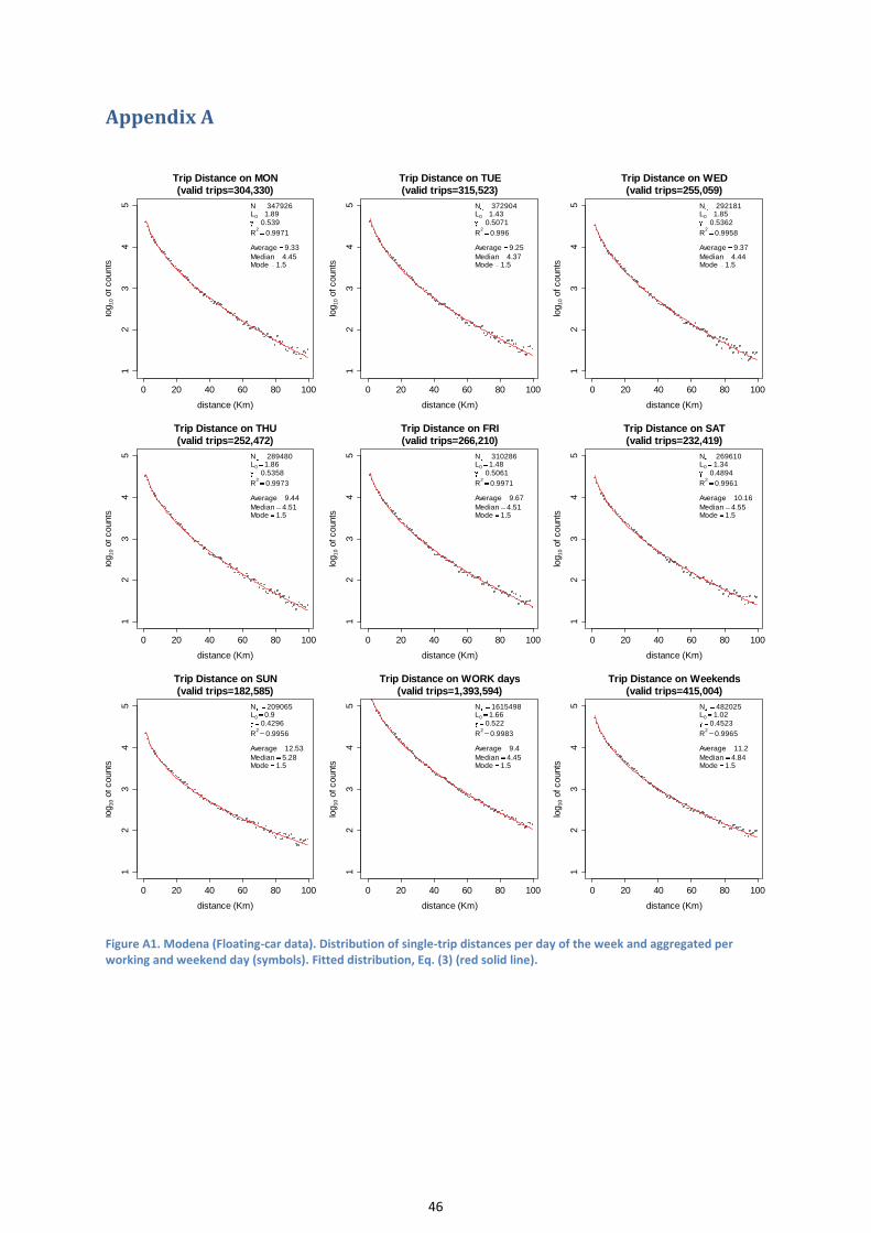
http://www.mitsubishi-motors.com/en/showroom/i-miev/specifications/

http://www.wunderground.com/history/

46

Appendix A

Figure A1. Modena (Floating-car data). Distribution of single-trip distances per day of the week and aggregated per working and weekend day (symbols). Fitted distribution, Eq. (3) (red solid line).

0 20 40 60 80 100

12

34

5

Trip Distance on MON


distance (Km)

log

10 o

f counts

N 347926L0 1.89

0.539

R2

0.9971

Average 9.33

Median 4.45Mode 1.5

0 20 40 60 80 100

12

34

5

Trip Distance on TUE


distance (Km)

log

10 o

f counts

N 372904L0 1.43

0.5071

R2

0.996

Average 9.25

Median 4.37Mode 1.5

0 20 40 60 80 100

12

34

5

Trip Distance on WED


distance (Km)

log

10 o

f counts

N 292181L0 1.85

0.5362

R2

0.9958

Average 9.37

Median 4.44Mode 1.5

0 20 40 60 80 100

12

34

5

Trip Distance on THU


distance (Km)

log

10 o

f counts

N 289480L0 1.86

0.5358

R2

0.9973

Average 9.44

Median 4.51Mode 1.5

0 20 40 60 80 100

12

34

5

Trip Distance on FRI


distance (Km)

log

10 o

f counts

N 310286L0 1.48

0.5061

R2

0.9971

Average 9.67

Median 4.51Mode 1.5

0 20 40 60 80 100

12

34

5

Trip Distance on SAT


distance (Km)

log

10 o

f counts

N 269610L0 1.34

0.4894

R2

0.9961

Average 10.16

Median 4.55Mode 1.5

0 20 40 60 80 100

12

34

5

Trip Distance on SUN


distance (Km)

log

10 o

f counts

N 209065L0 0.9

0.4296

R2

0.9956

Average 12.53

Median 5.28Mode 1.5

0 20 40 60 80 100

12

34

5


(valid trips=1,393,594)

distance (Km)

log

10 o

f counts

N 1615498L0 1.66

0.522

R2

0.9983

Average 9.4

Median 4.45Mode 1.5

0 20 40 60 80 100

12

34

5



distance (Km)

log

10 o

f counts

N 482025L0 1.02

0.4523

R2

0.9965

Average 11.2

Median 4.84Mode 1.5

47

Figure A2. Florence (Floating-car data). Distribution of single-trip distances per day of the week and aggregated per working and weekend day (symbols). Fitted distribution, Eq. (3) (red solid line).

0 20 40 60 80 100

12

34

5Trip Distance on MON


distance (Km)

log

10 o

f counts

N 277970L0 0.42

0.3988

R2

0.9934

Average 9.55

Median 4.24Mode 1.5

0 20 40 60 80 100

12

34

5



distance (Km)lo

g10 o

f counts

N 281195L0 0.49

0.4078

R2

0.9949

Average 9.59

Median 4.31Mode 1.5

0 20 40 60 80 100

12

34

5



distance (Km)

log

10 o

f counts

N 221617L0 0.59

0.4193

R2

0.9925

Average 9.71

Median 4.34Mode 1.5

0 20 40 60 80 100

12

34

5



distance (Km)

log

10 o

f counts

N 227801L0 0.52

0.4111

R2

0.9924

Average 9.69

Median 4.35Mode 1.5

0 20 40 60 80 100

12

34

5

Trip Distance on FRI


distance (Km)

log

10 o

f counts

N 236981L0 0.43

0.3979

R2

0.9922

Average 9.98

Median 4.36Mode 1.5

0 20 40 60 80 1001

23

45



distance (Km)

log

10 o

f counts

N 228675L0 0.08

0.3128

R2

0.9878

Average 10.82

Median 4.43Mode 1.5

0 20 40 60 80 100

12

34

5



distance (Km)

log

10 o

f counts

N 179941L0 0.05

0.2819

R2

0.9889

Average 13.87

Median 5.44Mode 1.5

0 20 40 60 80 100

12

34

5



distance (Km)

log

10 o

f counts

N 1248124L0 0.47

0.4048

R2

0.9952

Average 9.69

Median 4.32Mode 1.5

0 20 40 60 80 100

12

34

5



distance (Km)

log

10 o

f counts

N 411366L0 0.05

0.2917

R2

0.9896

Average 12.21

Median 4.85Mode 1.5

48

Figure A3. Floating-car data: Parameters of the fitted, single-trip distribution, Eq. (3). Modena (squares), Florence (circles). Red color denotes work days and their aggregate, blue weekend days and their aggregate. Vertical bars represent the standard error in the parameters estimate.

0.0e+00

5.0e+05

1.5e+06

2.0e+06

N

MON TUE WED THU FRI SAT SUN WORK days Weekends

-0.5

0.5

1.5

2.5

L0


0.0

0.2

0.4

0.6

0.8

1.0


49

Figure A4. Modena (Floating-car data): Number of daily trips per week day. Relative maxima occur usually at n=2 and n=4.

0 5 10 15 20

0.0

00.0

50.1

00.1

50.2

00.2

50.3

0Number of Daily Trips on MON


Number of trips

Rela

tive fre

quency

Average 4.59

Median 3.73

Mode 4.5

0 5 10 15 20

0.0

00.0

50.1

00.1

50.2

00.2

50.3

0

Number of Daily Trips on TUE


Number of tripsR

ela

tive fre

quency

Average 4.72

Median 3.85

Mode 4.5

0 5 10 15 20

0.0

00.0

50.1

00.1

50.2

00.2

50.3

0

Number of Daily Trips on WED


Number of trips

Rela

tive fre

quency

Average 4.76

Median 3.9

Mode 4.5

0 5 10 15 20

0.0

00.0

50.1

00.1

50.2

00.2

50.3

0

Number of Daily Trips on THU


Number of trips

Rela

tive fre

quency

Average 4.72

Median 3.85

Mode 4.5

0 5 10 15 20

0.0

00.0

50.1

00.1

50.2

00.2

50.3

0

Number of Daily Trips on FRI


Number of trips

Rela

tive fre

quency

Average 4.93

Median 4.06

Mode 4.5

0 5 10 15 200.0

00.0

50.1

00.1

50.2

00.2

50.3

0

Number of Daily Trips on SAT


Number of trips

Rela

tive fre

quency

Average 4.74

Median 3.84

Mode 2.5

0 5 10 15 20

0.0

00.0

50.1

00.1

50.2

00.2

50.3

0

Number of Daily Trips on SUN


Number of trips

Rela

tive fre

quency

Average 3.6

Median 2.7

Mode 2.5

0 5 10 15 20

0.0

00.0

50.1

00.1

50.2

00.2

50.3

0

Number of Daily Trips on WORK days


Number of trips

Rela

tive fre

quency

Average 4.74

Median 3.87

Mode 4.5

0 5 10 15 20

0.0

00.0

50.1

00.1

50.2

00.2

50.3

0

Number of Daily Trips on Weekends


Number of trips

Rela

tive fre

quency

Average 4.16

Median 3.23

Mode 2.5

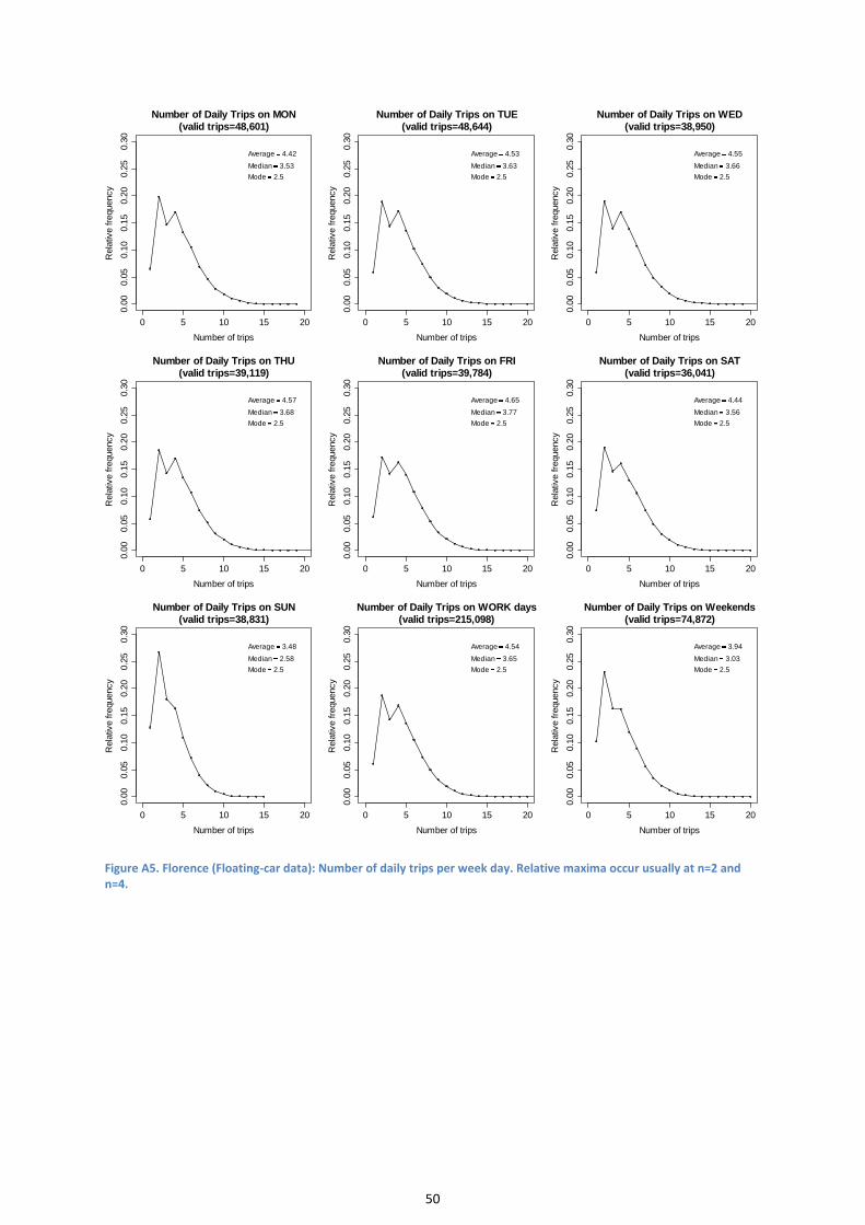
50

Figure A5. Florence (Floating-car data): Number of daily trips per week day. Relative maxima occur usually at n=2 and n=4.

0 5 10 15 20

0.0

00.0

50.1

00.1

50.2

00.2

50.3

0Number of Daily Trips on MON


Number of trips

Rela

tive fre

quency

Average 4.42

Median 3.53

Mode 2.5

0 5 10 15 20

0.0

00.0

50.1

00.1

50.2

00.2

50.3

0

Number of Daily Trips on TUE


Number of tripsR

ela

tive fre

quency

Average 4.53

Median 3.63

Mode 2.5

0 5 10 15 20

0.0

00.0

50.1

00.1

50.2

00.2

50.3

0

Number of Daily Trips on WED


Number of trips

Rela

tive fre

quency

Average 4.55

Median 3.66

Mode 2.5

0 5 10 15 20

0.0

00.0

50.1

00.1

50.2

00.2

50.3

0

Number of Daily Trips on THU


Number of trips

Rela

tive fre

quency

Average 4.57

Median 3.68

Mode 2.5

0 5 10 15 20

0.0

00.0

50.1

00.1

50.2

00.2

50.3

0

Number of Daily Trips on FRI


Number of trips

Rela

tive fre

quency

Average 4.65

Median 3.77

Mode 2.5

0 5 10 15 200.0

00.0

50.1

00.1

50.2

00.2

50.3

0

Number of Daily Trips on SAT


Number of trips

Rela

tive fre

quency

Average 4.44

Median 3.56

Mode 2.5

0 5 10 15 20

0.0

00.0

50.1

00.1

50.2

00.2

50.3

0

Number of Daily Trips on SUN


Number of trips

Rela

tive fre

quency

Average 3.48

Median 2.58

Mode 2.5

0 5 10 15 20

0.0

00.0

50.1

00.1

50.2

00.2

50.3

0

Number of Daily Trips on WORK days


Number of trips

Rela

tive fre

quency

Average 4.54

Median 3.65

Mode 2.5

0 5 10 15 20

0.0

00.0

50.1

00.1

50.2

00.2

50.3

0

Number of Daily Trips on Weekends


Number of trips

Rela

tive fre

quency

Average 3.94

Median 3.03

Mode 2.5

51

Figure A6. Modena (Floating-car data). Trip duration per week day and aggregated per working and weekend day (symbols). Fitted distribution, Eq. (10) (red solid line).

0 1 2 3 4 5 6

01

23

45

6

Trip Duration on MON


time (h)

log

10 o

f counts

T0 0.00360.36

N 596362

R2

0.9895

Average 0.26

Median 0.21Arg Max 0.12

0 1 2 3 4 5 6

01

23

45

6

Trip Duration on TUE


time (h)

log

10 o

f counts

T0 0.00290.35

N 638442

R2

0.986

Average 0.26


0 1 2 3 4 5 6

01

23

45

6

Trip Duration on WED


time (h)

log

10 o

f counts

T0 0.00970.41

N 403639

R2

0.9839

Average 0.26


0 1 2 3 4 5 6

01

23

45

6

Trip Duration on THU


time (h)

log

10 o

f counts

T0 0.00480.37

N 461692

R2

0.9855

Average 0.26


0 1 2 3 4 5 6

01

23

45

6

Trip Duration on FRI


time (h)

log

10 o

f counts

T0 0.01310.42

N 387432

R2

0.9853

Average 0.27


0 1 2 3 4 5 6

01

23

45

6

Trip Duration on SAT


time (h)

log

10 o

f counts

T0 0.04970.54

N 295806

R2

0.9881

Average 0.27


0 1 2 3 4 5 6

01

23

45

6

Trip Duration on SUN


time (h)

log

10 o

f counts

T0 0.15650.68

N 167781

R2

0.9859

Average 0.31


0 1 2 3 4 5 6

01

23

45

6

Trip Duration on WORK days

(valid trips=1,398,143)

time (h)

log

10 o

f counts

T0 0.00590.38

N 2421075

R2

0.992

Average 0.26


0 1 2 3 4 5 6

01

23

45

6

Trip Duration on Weekends


time (h)

log

10 o

f counts

T0 0.12760.66

N 394528

R2

0.9921

Average 0.28


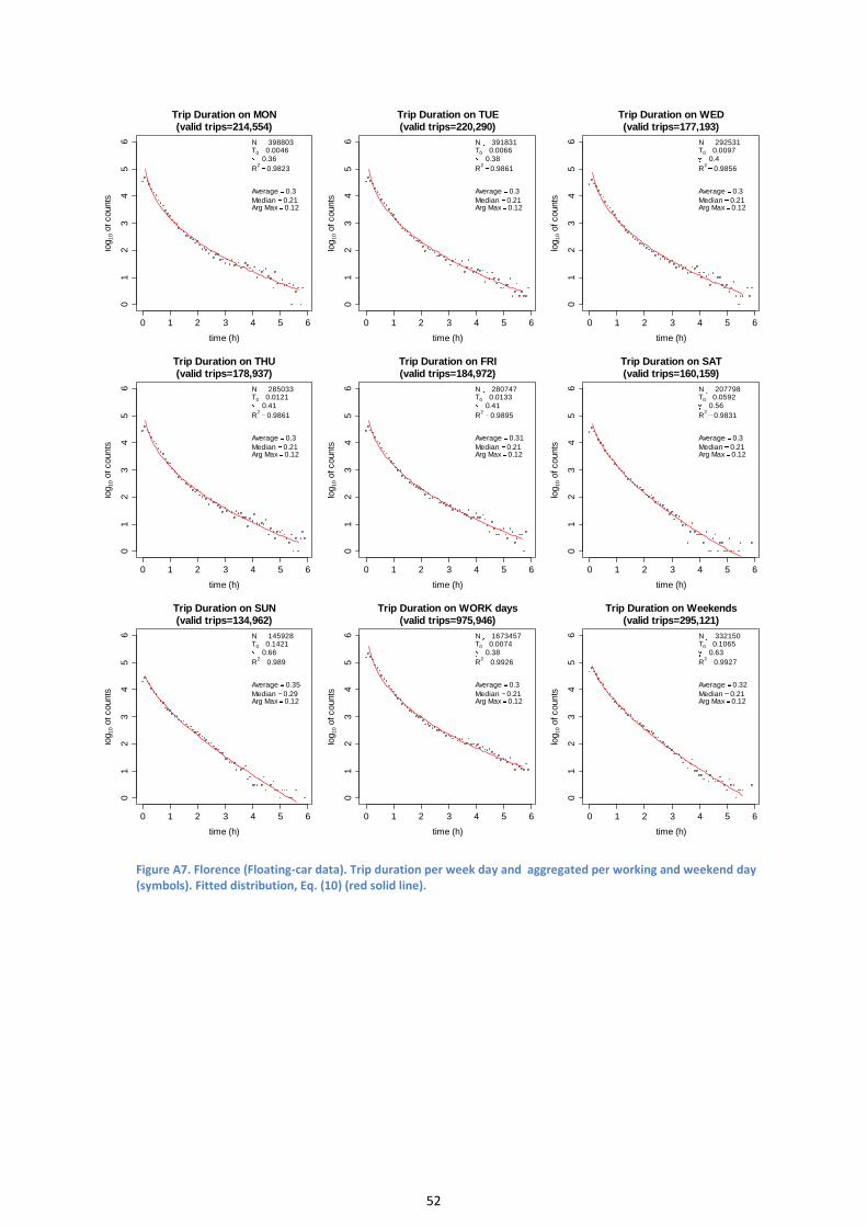
52

Figure A7. Florence (Floating-car data). Trip duration per week day and aggregated per working and weekend day (symbols). Fitted distribution, Eq. (10) (red solid line).

0 1 2 3 4 5 6

01

23

45

6Trip Duration on MON


time (h)

log

10 o

f counts

T0 0.00460.36

N 398803

R2

0.9823

Average 0.3


0 1 2 3 4 5 6

01

23

45

6

Trip Duration on TUE


time (h)lo

g10 o

f counts

T0 0.00660.38

N 391831

R2

0.9861

Average 0.3


0 1 2 3 4 5 6

01

23

45

6

Trip Duration on WED


time (h)

log

10 o

f counts

T0 0.00970.4

N 292531

R2

0.9856

Average 0.3


0 1 2 3 4 5 6

01

23

45

6

Trip Duration on THU


time (h)

log

10 o

f counts

T0 0.01210.41

N 285033

R2

0.9861

Average 0.3


0 1 2 3 4 5 6

01

23

45

6

Trip Duration on FRI


time (h)

log

10 o

f counts

T0 0.01330.41

N 280747

R2

0.9895

Average 0.31


0 1 2 3 4 5 60

12

34

56

Trip Duration on SAT


time (h)

log

10 o

f counts

T0 0.05920.56

N 207798

R2

0.9831

Average 0.3


0 1 2 3 4 5 6

01

23

45

6

Trip Duration on SUN


time (h)

log

10 o

f counts

T0 0.14210.66

N 145928

R2

0.989

Average 0.35


0 1 2 3 4 5 6

01

23

45

6

Trip Duration on WORK days


time (h)

log

10 o

f counts

T0 0.00740.38

N 1673457

R2

0.9926

Average 0.3


0 1 2 3 4 5 6

01

23

45

6

Trip Duration on Weekends


time (h)

log

10 o

f counts

T0 0.10650.63

N 332150

R2

0.9927

Average 0.32


53

Figure A8. Modena (Floating-car data). Observed (symbols) and modelled (red solid line, Eq. (3)) work-trip distance distribution per week day and aggregated per work and weekend day.

0 20 40 60 80 100

01

23

4Work-Trip Distance on MON


distance (Km)

log

10 o

f counts

L0 5.380.68

N 14237

R2

0.9448


0 20 40 60 80 100

01

23

4

Work-Trip Distance on TUE


distance (Km)lo

g10 o

f counts

L0 6.610.76

N 14224

R2

0.9654


0 20 40 60 80 100

01

23

4

Work-Trip Distance on WED


distance (Km)

log

10 o

f counts

L0 7.260.77

N 11455

R2

0.9665


0 20 40 60 80 100

01

23

4

Work-Trip Distance on THU


distance (Km)

log

10 o

f counts

L0 6.550.74

N 12296

R2

0.9714


0 20 40 60 80 100

01

23

4

Work-Trip Distance on FRI


distance (Km)

log

10 o

f counts

L0 4.740.65

N 12110

R2

0.9584


0 20 40 60 80 1000

12

34

Work-Trip Distance on SAT

(valid trips=8,917)

distance (Km)

log

10 o

f counts

L0 1.630.5

N 9745

R2

0.9429


0 20 40 60 80 100

01

23

4

Work-Trip Distance on SUN

(valid trips=7,227)

distance (Km)

log

10 o

f counts

L0 2.030.5

N 7392

R2

0.9442


0 20 40 60 80 100

01

23

4

Work-Trip Distance on WORK days


distance (Km)

log

10 o

f counts

L0 7.090.76

N 63442

R2

0.9811


0 20 40 60 80 100

01

23

4

Work-Trip Distance on Weekends


distance (Km)

log

10 o

f counts

L0 1.930.51

N 16987

R2

0.9557


54

Figure A9. Florence (Floating-car data). Observed (symbols) and modelled (red solid line, Eq. (3)), work-trip distance distribution per week day and aggregated per work and weekend day.

0 20 40 60 80 100

01

23

4Work-Trip Distance on MON

(valid trips=9,663)

distance (Km)

log

10 o

f counts

L0 4.040.61

N 10102

R2

0.928


0 20 40 60 80 100

01

23

4

Work-Trip Distance on TUE

(valid trips=9,511)

distance (Km)lo

g10 o

f counts

L0 4.420.63

N 9828

R2

0.9468


0 20 40 60 80 100

01

23

4

Work-Trip Distance on WED

(valid trips=7,919)

distance (Km)

log

10 o

f counts

L0 3.150.58

N 8424

R2

0.9409


0 20 40 60 80 100

01

23

4

Work-Trip Distance on THU

(valid trips=8,408)

distance (Km)

log

10 o

f counts

L0 3.150.59

N 9080

R2

0.9189


0 20 40 60 80 100

01

23

4

Work-Trip Distance on FRI

(valid trips=8,366)

distance (Km)

log

10 o

f counts

L0 4.720.66

N 8768

R2

0.9475


0 20 40 60 80 1000

12

34

Work-Trip Distance on SAT

(valid trips=5,808)

distance (Km)

log

10 o

f counts

L0 0.740.42

N 6431

R2

0.924


0 20 40 60 80 100

01

23

4

Work-Trip Distance on SUN

(valid trips=5,066)

distance (Km)

log

10 o

f counts

L0 0.650.39

N 5313

R2

0.9128


0 20 40 60 80 100

01

23

4

Work-Trip Distance on WORK days


distance (Km)

log

10 o

f counts

L0 4.190.62

N 45880

R2

0.9702


0 20 40 60 80 100

01

23

4

Work-Trip Distance on Weekends


distance (Km)

log

10 o

f counts

L0 0.840.42

N 11626

R2

0.9274


55

Figure A10. Modena (Floating-car data). Trip duration of work trips per day and aggregate per working and weekend day (symbols). Red solid line fitted distribution, Eq. (10).

0 1 2 3 4 5

01

23

45

Work-Trip Duration on MON


time (h)

log

10 o

f counts

T0 0.01410.42

N 21225

R2

0.97

Average 0.32


0 1 2 3 4 50

12

34

5

Work-Trip Duration on TUE


time (h)

log

10 o

f counts

T0 0.0670.6

N 18260

R2

0.97

Average 0.29


0 1 2 3 4 5

01

23

45

Work-Trip Duration on WED


time (h)

log

10 o

f counts

T0 0.03890.52

N 16426

R2

0.97

Average 0.29


0 1 2 3 4 5

01

23

45

Work-Trip Duration on THU


time (h)

log

10 o

f counts

T0 0.03410.51

N 18226

R2

0.96

Average 0.29


0 1 2 3 4 5

01

23

45

Work-Trip Duration on FRI


time (h)

log

10 o

f counts

T0 0.07070.61

N 15549

R2

0.97

Average 0.29


0 1 2 3 4 5

01

23

45

Work-Trip Duration on SAT

(valid trips=8,986)

time (h)

log

10 o

f counts

T0 0.01070.4

N 13898

R2

0.96

Average 0.28


0 1 2 3 4 5

01

23

45

Work-Trip Duration on SUN

(valid trips=7,328)

time (h)

log

10 o

f counts

T0 0.11340.6

N 7387

R2

0.96

Average 0.35


0 1 2 3 4 5

01

23

45

Work-Trip Duration on WORK days


time (h)

log

10 o

f counts

T0 0.06280.58

N 81273

R2

0.98

Average 0.3


0 1 2 3 4 5

01

23

45

Work-Trip Duration on Weekends


time (h)

log

10 o

f counts

T0 0.05710.53

N 18388

R2

0.98

Average 0.31


56

Figure A11. Florence (Floating-car data). Trip duration of work trips per day and aggregate per working and weekend day (symbols). Red solid line fitted distribution, Eq. (10).

0 1 2 3 4 5

01

23

45

Work-Trip Duration on MON

(valid trips=9,726)

time (h)

log

10 o

f counts

T0 0.11670.65

N 11728

R2

0.97

Average 0.36


0 1 2 3 4 5

01

23

45

Work-Trip Duration on TUE

(valid trips=9,544)

time (h)lo

g10 o

f counts

T0 0.08150.61

N 12602

R2

0.95

Average 0.33

Median 0.2Mode 0.12

0 1 2 3 4 5

01

23

45

Work-Trip Duration on WED

(valid trips=7,938)

time (h)

log

10 o

f counts

T0 0.04620.55

N 12004

R2

0.94

Average 0.32

Median 0.2Mode 0.12

0 1 2 3 4 5

01

23

45

Work-Trip Duration on THU

(valid trips=8,428)

time (h)

log

10 o

f counts

T0 0.04920.55

N 12429

R2

0.95

Average 0.33

Median 0.2Mode 0.12

0 1 2 3 4 5

01

23

45

Work-Trip Duration on FRI

(valid trips=8,396)

time (h)

log

10 o

f counts

T0 0.05340.55

N 11617

R2

0.96

Average 0.33

Median 0.2Mode 0.12

0 1 2 3 4 50

12

34

5

Work-Trip Duration on SAT

(valid trips=5,836)

time (h)

log

10 o

f counts

T0 0.08450.59

N 6671

R2

0.98

Average 0.32


0 1 2 3 4 5

01

23

45

Work-Trip Duration on SUN

(valid trips=5,110)

time (h)

log

10 o

f counts

T0 0.21520.73

N 5062

R2

0.96

Average 0.37


0 1 2 3 4 5

01

23

45

Work-Trip Duration on WORK days


time (h)

log

10 o

f counts

T0 0.10260.65

N 55557

R2

0.97

Average 0.34


0 1 2 3 4 5

01

23

45

Work-Trip Duration on Weekends


time (h)

log

10 o

f counts

T0 0.13230.64

N 11563

R2

0.98

Average 0.35


57

Figure A12. Modena (top) and Florence (bottom) (Floating car data). Distribution of travel speeds: average speed, motion speed (obtained by removing intermediate stops), and the segment speed.

0 50 100 150

0.0

00

0.0

05

0.0

10

0.0

15

0.0

20

0.0

25

0.0

30

Trip Average Speed (circles), Trip Motion Speed (squares) and Segment Speed (triangles)

Modena, valid trips: 1,814,529 - valid segments: 12,758,863

Speed (km/h)

Re

lative

Fre

qu

en

cy

0 50 100 150

0.0

00

0.0

05

0.0

10

0.0

15

0.0

20

0.0

25

0.0

30

0 50 100 150

0.0

00

0.0

05

0.0

10

0.0

15

0.0

20

0.0

25

0.0

30 Average Speed Distr.:

Average 30.19

Median 28.5

Max at 18.5

Average Motion Speed Distr.:

Average 31.16

Median 29.5

Max at 18.5

Segment Speed Distr.:

Average 57.55

Median 52.5

Max at 0.5

0 50 100 150

0.0

00

0.0

05

0.0

10

0.0

15

0.0

20

0.0

25

0.0

30

Trip Average Speed (circles), Trip Motion Speed (squares) and Segment Speed (triangles)

Firenze, valid trips: 1,269,519 - valid segments: 29,548,917

Speed (km/h)

Re

lative

Fre

qu

en

cy

0 50 100 150

0.0

00

0.0

05

0.0

10

0.0

15

0.0

20

0.0

25

0.0

30

0 50 100 150

0.0

00

0.0

05

0.0

10

0.0

15

0.0

20

0.0

25

0.0

30 Average Speed Distr.:

Average 27.28

Median 24.5

Max at 18.5

Average Motion Speed Distr.:

Average 28.14

Median 25.5

Max at 19.5

Segment Speed Distr.:

Average 42.9

Median 37.5

Max at 36.5

58

Figure A13. Green eMotion data: Trip distance per week day and aggregated per working and weekend day.

0 50 100 150

01

23

4Trip Distance on MON

(GeM_ALL_v2, valid trips=10,336)

distance (Km)

log

10 o

f counts


0 50 100 150

01

23

4



distance (Km)lo

g10 o

f counts


0 50 100 150

01

23

4



distance (Km)

log

10 o

f counts


0 50 100 150

01

23

4



distance (Km)

log

10 o

f counts


0 50 100 150

01

23

4Trip Distance on FRI


distance (Km)

log

10 o

f counts


0 50 100 150

01

23

4



distance (Km)

log

10 o

f counts


0 50 100 150

01

23

4



distance (Km)

log

10 o

f counts


0 50 100 150

01

23

4



distance (Km)

log

10 o

f counts


0 50 100 150

01

23

4



distance (Km)

log

10 o

f counts


59

Figure A14. Green eMotion data: Observed daily mobility length distribution and fitted distribution, Eq. (6), per week day.

0 50 100 150

0.0

0.5

1.0

1.5

2.0

2.5

3.0

Daily Mobility Length on MON

(daily activities=2,289)

distance (Km)

log

10 o

f counts

y0 22.6L0 20.67

0.55

R2

0.9555

Average 33


0 50 100 1500.0

0.5

1.0

1.5

2.0

2.5

3.0

Daily Mobility Length on TUE


distance (Km)

log

10 o

f counts

y0 20.05L0 20.81

0.59

R2

0.9193

Average 33.7


0 50 100 150

0.0

0.5

1.0

1.5

2.0

2.5

3.0

Daily Mobility Length on WED


distance (Km)

log

10 o

f counts

y0 23.12L0 20.01

0.57

R2

0.928

Average 33.8

Median 27.8Mode 4.5

0 50 100 150

0.0

0.5

1.0

1.5

2.0

2.5

3.0

Daily Mobility Length on THU


distance (Km)

log

10 o

f counts

y0 16.43L0 19.2

0.7

R2

0.9434

Average 33.4


0 50 100 150

0.0

0.5

1.0

1.5

2.0

2.5

3.0

Daily Mobility Length on FRI


distance (Km)

log

10 o

f counts

y0 21.95L0 20.85

0.56

R2

0.9525

Average 33.1


0 50 100 150

0.0

0.5

1.0

1.5

2.0

2.5

3.0

Daily Mobility Length on SAT


distance (Km)

log

10 o

f counts

y0 6.53L0 17.4

0.86

R2

0.9491

Average 34.8


0 50 100 150

0.0

0.5

1.0

1.5

2.0

2.5

3.0

Daily Mobility Length on SUN


distance (Km)

log

10 o

f counts

y0 11.24L0 19.8

0.59

R2

0.9107

Average 32.9

Median 26.6Mode 6.5

0 50 100 150

0.0

0.5

1.0

1.5

2.0

2.5

3.0

Daily Mobility Length on WORK days


distance (Km)

log

10 o

f counts

y0 107.41L0 20.69

0.58

R2

0.9694

Average 33.4


0 50 100 150

0.0

0.5

1.0

1.5

2.0

2.5

3.0

Daily Mobility Length on Weekends


distance (Km)

log

10 o

f counts

y0 17.54L0 18.74

0.71

R2

0.9606

Average 33.9

Median 27.8Mode 6.5

60

Figure A15. Electric energy consumption per km (Denmark) during the year: 1=Jan to 12=Dec.

Figure A16. Electric energy consumption per km (Ireland) during the year: 1=Jan to 12=Dec.

0.1 0.2 0.3 0.4 0.5

010

20

30

40

DK Month: 1

(valid trips=1456)

Energy per distance (kWh/km)

counts

W_AVE 0.2564

MED 0.248

0.1 0.2 0.3 0.4 0.5

010

20

30

40

DK Month: 2

(valid trips=1418)


counts

W_AVE 0.2523

MED 0.2401

0.1 0.2 0.3 0.4 0.5

010

20

30

40

DK Month: 3

(valid trips=1449)


counts

W_AVE 0.2466

MED 0.2371

0.1 0.2 0.3 0.4 0.5

010

20

30

40

DK Month: 4

(valid trips=1737)


counts

W_AVE 0.2312

MED 0.2102

0.1 0.2 0.3 0.4 0.5

010

20

30

40

DK Month: 5

(valid trips=1945)


counts

W_AVE 0.1954

MED 0.1725

0.1 0.2 0.3 0.4 0.5

010

20

30

40

DK Month: 6

(valid trips=1660)


counts

W_AVE 0.2015

MED 0.1743

0.1 0.2 0.3 0.4 0.5

010

20

30

40

DK Month: 7

(valid trips=1964)


counts

W_AVE 0.1439

MED 0.1313

0.1 0.2 0.3 0.4 0.5

010

20

30

40

DK Month: 8

(valid trips=2238)


counts

W_AVE 0.1443

MED 0.1334

0.1 0.2 0.3 0.4 0.5

010

20

30

40

DK Month: 9

(valid trips=2069)


counts

W_AVE 0.1669

MED 0.1499

0.1 0.2 0.3 0.4 0.5

010

20

30

40

DK Month: 10

(valid trips=2328)


counts

W_AVE 0.2029

MED 0.1923

0.1 0.2 0.3 0.4 0.5

010

20

30

40

DK Month: 11

(valid trips=2178)


counts

W_AVE 0.2257

MED 0.2131

0.1 0.2 0.3 0.4 0.5

010

20

30

40

DK Month: 12

(valid trips=1223)


counts

W_AVE 0.2593

MED 0.2476

0.1 0.2 0.3 0.4 0.5

010

20

30

40

IE Month: 1

(valid trips=1249)


counts

W_AVE 0.2357

MED 0.2188

0.1 0.2 0.3 0.4 0.5

010

20

30

40

IE Month: 2

(valid trips=1061)


counts

W_AVE 0.2293

MED 0.2082

0.1 0.2 0.3 0.4 0.5

010

20

30

40

IE Month: 3

(valid trips=1134)


counts

W_AVE 0.2179

MED 0.1943

0.1 0.2 0.3 0.4 0.5

010

20

30

40

IE Month: 4

(valid trips=920)


counts

W_AVE 0.2055

MED 0.1842

0.1 0.2 0.3 0.4 0.5

010

20

30

40

IE Month: 5

(valid trips=951)


counts

W_AVE 0.1952

MED 0.1708

0.1 0.2 0.3 0.4 0.5

010

20

30

40

IE Month: 6

(valid trips=446)


counts

W_AVE 0.1889

MED 0.1651

0.1 0.2 0.3 0.4 0.5

010

20

30

40

IE Month: 7

(valid trips=1044)


counts

W_AVE 0.1921

MED 0.1586

0.1 0.2 0.3 0.4 0.5

010

20

30

40

IE Month: 8

(valid trips=1195)


counts

W_AVE 0.1885

MED 0.1609

0.1 0.2 0.3 0.4 0.5

010

20

30

40

IE Month: 9

(valid trips=1267)


counts

W_AVE 0.1896

MED 0.1669

0.1 0.2 0.3 0.4 0.5

010

20

30

40

IE Month: 10

(valid trips=1423)


counts

W_AVE 0.1964

MED 0.1762

0.1 0.2 0.3 0.4 0.5

010

20

30

40

IE Month: 11

(valid trips=1509)


counts

W_AVE 0.2096

MED 0.1901

0.1 0.2 0.3 0.4 0.5

010

20

30

40

IE Month: 12

(valid trips=629)


counts

W_AVE 0.2377

MED 0.2208

61

Figure A17. Electric energy consumption per km (Spain) during the year: 1=Jan to 12=Dec.

Figure A18. Electric energy consumption per km (Sweden) during the year: 1=Jan to 12=Dec.

0.1 0.2 0.3 0.4 0.5

010

20

30

40

ES Month: 1

(valid trips=807)


counts

W_AVE 0.2414

MED 0.2324

0.1 0.2 0.3 0.4 0.5

010

20

30

40

ES Month: 2

(valid trips=572)


counts

W_AVE 0.2463

MED 0.2322

0.1 0.2 0.3 0.4 0.5

010

20

30

40

ES Month: 3

(valid trips=627)


counts

W_AVE 0.2263

MED 0.2149

0.1 0.2 0.3 0.4 0.5

010

20

30

40

ES Month: 4

(valid trips=510)


counts

W_AVE 0.2231

MED 0.2173

0.1 0.2 0.3 0.4 0.5

010

20

30

40

ES Month: 5

(valid trips=727)


counts

W_AVE 0.218

MED 0.2101

0.1 0.2 0.3 0.4 0.5

010

20

30

40

ES Month: 6

(valid trips=844)


counts

W_AVE 0.2219

MED 0.2047

0.1 0.2 0.3 0.4 0.5

010

20

30

40

ES Month: 7

(valid trips=767)


counts

W_AVE 0.2283

MED 0.2148

0.1 0.2 0.3 0.4 0.5

010

20

30

40

ES Month: 8

(valid trips=354)


counts

W_AVE 0.2276

MED 0.2123

0.1 0.2 0.3 0.4 0.5

010

20

30

40

ES Month: 9

(valid trips=656)


counts

W_AVE 0.2239

MED 0.2095

0.1 0.2 0.3 0.4 0.5

010

20

30

40

ES Month: 10

(valid trips=1135)


counts

W_AVE 0.2305

MED 0.2202

0.1 0.2 0.3 0.4 0.5

010

20

30

40

ES Month: 11

(valid trips=589)


counts

W_AVE 0.2711

MED 0.2688

0.1 0.2 0.3 0.4 0.5

010

20

30

40

ES Month: 12

(valid trips=649)


counts

W_AVE 0.2356

MED 0.2238

0.0 0.2 0.4 0.6 0.8 1.0

010

20

30

40

SE Month: 1

(valid trips=264)


counts

W_AVE 0.2822

MED 0.2746

0.0 0.2 0.4 0.6 0.8 1.0

010

20

30

40

SE Month: 2

(valid trips=278)


counts

W_AVE 0.2719

MED 0.2605

0.0 0.2 0.4 0.6 0.8 1.0

010

20

30

40

SE Month: 3

(valid trips=298)


counts

W_AVE 0.24

MED 0.2255

0.0 0.2 0.4 0.6 0.8 1.0

010

20

30

40

SE Month: 4

(valid trips=539)


counts

W_AVE 0.1859

MED 0.1745

0.0 0.2 0.4 0.6 0.8 1.0

010

20

30

40

SE Month: 5

(valid trips=822)


counts

W_AVE 0.1512

MED 0.1394

0.0 0.2 0.4 0.6 0.8 1.0

010

20

30

40

SE Month: 6

(valid trips=348)


counts

W_AVE 0.1432

MED 0.1357

0.0 0.2 0.4 0.6 0.8 1.0

010

20

30

40

SE Month: 7

(valid trips=620)


counts

W_AVE 0.1382

MED 0.1302

0.0 0.2 0.4 0.6 0.8 1.0

010

20

30

40

SE Month: 8

(valid trips=631)


counts

W_AVE 0.1392

MED 0.1317

0.0 0.2 0.4 0.6 0.8 1.0

010

20

30

40

SE Month: 9

(valid trips=731)


counts

W_AVE 0.1506

MED 0.1314

0.0 0.2 0.4 0.6 0.8 1.0

010

20

30

40

SE Month: 10

(valid trips=0)


counts

W_AVE NaN

MED NA

0.0 0.2 0.4 0.6 0.8 1.0

010

20

30

40

SE Month: 11

(valid trips=440)


counts

W_AVE 0.2184

MED 0.2035

0.0 0.2 0.4 0.6 0.8 1.0

010

20

30

40

SE Month: 12

(valid trips=205)


counts

W_AVE 0.298

MED 0.2859

62

Appendix B

The output of the Java processing code is:

1. Motion state versus GPS signal quality (SG= “Signal Goodness”) table for Modena (top) and Florence

(bottom);

Modena MS=0 (engine on) MS=1 (motion) MS=2 (engine off)

SG=1 (no signal) 260,416 0 240,158

SG=2 (weak signal) 26,776 124,314 30,189

SG=3 (good signal) 1,810,912 11,135,176 1,826,986

Anomalous events with full trip removal: 7.24%

Florence MS=0 (engine on) MS=1 (motion) MS=2 (engine off)

SG=1 (no signal) 166,414 0 141,168

SG=2 (weak signal) 23,011 636,764 26,562

SG=3 (good signal) 1,289,409 28,493,205 1,310,194

Anomalous events with full trip removal: 4.95%

2. Cleaned version of the original dataset, after removal of the inconsistent (anomalous) events/trips, as

defined above;

3. Detailed information on the anomalous trips and stops filtered out;

4. Summary statistics, like the one presented in Table 1;

5. Distributions and statistics files, log/control files, for a total of approximately 95 output files;

6. A file with stop times not aggregated into a histogram (used for some MATLAB calculations).

63

Europe Direct is a service to help you find answers to your questions about the European Union

Freephone number (*): 00 800 6 7 8 9 10 11

(*) Certain mobile telephone operators do not allow access to 00 800 numbers or these calls may be billed.

A great deal of additional information on the European Union is available on the Internet.

It can be accessed through the Europa server http://europa.eu.

How to obtain EU publications

Our publications are available from EU Bookshop (http://bookshop.europa.eu),

where you can place an order with the sales agent of your choice.

The Publications Office has a worldwide network of sales agents.

You can obtain their contact details by sending a fax to (352) 29 29-42758.

European Commission

EUR 27468 EN – Joint Research Centre – Institute for Energy and Transport

Title: Individual mobility: From conventional to electric cars

Author(s): Alberto V. Donati, Panagiota Dilara*, Christian Thiel, Alessio Spadaro, Dimitrios Gkatzoflias, Yannis Drossinos

European Commission, Joint Research Centre, T.P. 441, Via Enrico Fermi, I-21027 Ispra (VA), Italy

*Current address: European Commission, DG GROW, BRU-BREY 10/030, B-1049 Bruxelles, Belgium

Luxembourg: Publications Office of the European Union

2015 – 66 pp. – 21.0 x 29.7 cm

EUR – Scientific and Technical Research series – ISSN 1831-9424 (online), ISSN 1018-5593 (print)

ISBN 978-92-79-51894-2 (PDF)

ISBN 978-92-79-51895-9 (print)

doi:10.2790/405373 (online)

ISBN 978-92-79-51894-2

doi:10.2790/405373

JRC Mission As the Commission’s in-house science service, the Joint Research Centre’s mission is to provide EU policies with independent, evidence-based scientific and technical support throughout the whole policy cycle. Working in close cooperation with policy Directorates-General, the JRC addresses key societal challenges while stimulating innovation through developing new methods, tools and standards, and sharing its know-how with the Member States, the scientific community and international partners.

Serving society Stimulating innovation Supporting legislation

LD

-NA

-27

46

8-E

N-N

Documents

Individual mobility: From conventional to electric carspublications.jrc.ec.europa.eu/repository/bitstream/... · data were collected through a Web-based travel diary, 24 hours per