Embed Size (px)
Citation preview
Indiscernibility and Vagueness in SpatialInformation Systems
Karim Oukbir
Stockholm 2003
Doctoral Dissertation
Royal Institute of Technology
Department of Numerical Analysis and Computer Science

Akademisk avhandling som med tillstånd av Kungl Tekniska Högskolan framläggestill offentlig granskning för avläggande av teknologie doktorsexamen 10 novem-ber 2003 kl 13.00 i Kollegiesalen, Administrationsbyggnaden, Kungl Tekniska Hög-skolan, Valhallavägen 79, Stockholm.
ISBN 91-7283-602-4TRITA-NA-0321ISSN 0348-2952ISRN KTH/NA/R-03/21-SE
© Karim Oukbir, October 2003
Universitetsservice US AB, Stockholm 2003
Abstract
We investigate the use of the concept of indiscernibility and vagueness in spatialinformation systems. To represent indiscernibility and vagueness we use rough sets,respectively fuzzy sets.
We introduce a theoretical model to support approximate queries in informationsystems and we show how those queries can be used to perform uncertain classific-ations. We also explore how to assess quality of uncertain classifications and waysto compare those classifications to each other in order to assess accuracies.
We implement the query language in an SQL relational language to demonstratethe feasibility of approximate queries and we perform an experiment on real datausing uncertain classifications.
ISBN 91-7283-602-4 • TRITA-NA-0321 • ISSN 0348-2952 • ISRN KTH/NA/R-03/21-SE
iii

iv

Sammanfattning
Vi undersöker användningen av begreppen oskiljbarhet och vaghet i spatiella infor-mationssystem. Vi använder oss av grova mängder (rough sets) för att modelleraoskiljbarhet och oskarpa mängder (fuzzy sets) för att modellera vaghet.
Vi definierar en teoretisk modell för ett frågespråk som hanterar osäker informa-tion, och med hjälp av denna modell introducerar vi ett nytt sätt att utföra osäkraklassificeringar. Vi undersöker också nya sätt att mäta och jämföra noggrannhetenhos osäkra data.
Vi implementerar vår modell i ett SQL-baserat frågespråk för att undersökamöjligheten att utföra approximativa frågor i informationssystemet samt genomförslutligen ett experiment med verkliga data.
ISBN 91-7283-602-4 • TRITA-NA-0321 • ISSN 0348-2952 • ISRN KTH/NA/R-03/21-SE
v

vi

Résumé
Nous explorons l’utilisation de la notion d’indiscernabilité et celle de la notion duflou dans les systèmes d’information spatiales. Nous utilison la théorie des ensemblesapproximatifs pour modeler l’indiscernabilité des éléments de l’univers et la théoriedes ensembles flous pour la representation de l’information floue.
Nous introduisons un modèle théorique qui permet d’implémenter les interro-gations approximatifs dans les systèmes d’information. Ce nouveau langage permetde définir le concept de classification incertaines. De plus, nous explorons les moyende calculer et de comparer les degrés d’exactitudes de ces classifications.
Nous implementons ce langage d’interrogation à l’aide d’un langage de requêteSQL pour démontrer la faisabilite de notre idée et nous effectuons des expériencessur des données réels.
ISBN 91-7283-602-4 • TRITA-NA-0321 • ISSN 0348-2952 • ISRN KTH/NA/R-03/21-SE
vii

viii
Acknowledgments
First of all I would like to thank my supervisor Per Svensson for his unlimited helpand his support, for insightful discussions on the ideas of this thesis, and for quickfeedback on my manuscripts. Without Per this thesis would not have been.
I also thank Stefan Arnborg, my secondary supervisor, for his help and hissupport.
Ola Ahlqvist and Johannes Keukelaar for our joint papers, collaborating withthem has always been a pleasure. It was also a great help to be able to discuss withJohannes some of the ideas of this manuscript.
Mike Worboys was the opponent for my licentiate degree in June 2001. Thediscussions I had the opportunity to have with him, both here in Stockholm and inNorway during the ScanGIS’2001 conference, have been a great help when preparingmy doctoral thesis. Thank you Mike!
Johannes Keukelaar (again), Jesper Fredriksson, Klas Wallenius and ÖjvindJohansson for great time past here.
I am grateful to Lars Engebretsen who has helped me with LATEX matters whenwriting this manuscript. All the other members of my research group, those thatare still in the group and those that have left it, they all have been very helpful tome.
I wish to thank Yiyu Yao who, through email, has helped me understand-ing some issues related to interval sets and rough sets. Tore Risch and TimourKatchaounov for many fruitful discussions and their help with the AMOS II sys-tem. Ralf Hartmut Güting and his group for interesting discussions in the beginningof my thesis work.
I also thank the former Center for Geoinformatics, Stockholm and the SwedishDefense Research Agency (FOI) for providing fundings for this research. The Taylor& Francis Group (www.tandf.co.uk) for kindly allowing me to reuse the materialspresented in 7.3 from our paper [AKO03].
My parents, my sister and my cousin Omar, thank you for your support.
My lo♥ely fiancé Jennie, thank you for your infinite patience!
ix

x
Contents
1 Introduction 11.1 Contributions . . . . . . . . . . . . . . . . . . . . . . . . . . . . . . 4
2 Uncertainty Representation 52.1 An Ontology of Imperfection . . . . . . . . . . . . . . . . . . . . . 52.2 Fuzzy Sets . . . . . . . . . . . . . . . . . . . . . . . . . . . . . . . . 62.3 Rough Sets . . . . . . . . . . . . . . . . . . . . . . . . . . . . . . . 72.4 Marek’s Model . . . . . . . . . . . . . . . . . . . . . . . . . . . . . 82.5 Rough Fuzzy Extension of Marek’s Model . . . . . . . . . . . . . . 82.6 The Egg-Yolk Model . . . . . . . . . . . . . . . . . . . . . . . . . . 92.7 Other Models . . . . . . . . . . . . . . . . . . . . . . . . . . . . . . 102.8 Conclusion . . . . . . . . . . . . . . . . . . . . . . . . . . . . . . . 10
3 Indiscernibility and Vagueness 133.1 Approximation of Sets . . . . . . . . . . . . . . . . . . . . . . . . . 133.2 Truth Functionality and Rough Sets . . . . . . . . . . . . . . . . . 15
3.2.1 Families of Subsets . . . . . . . . . . . . . . . . . . . . . . . 163.2.2 Interval Sets . . . . . . . . . . . . . . . . . . . . . . . . . . 173.2.3 Restriction of Approximations . . . . . . . . . . . . . . . . 18
3.3 Fuzzy Sets . . . . . . . . . . . . . . . . . . . . . . . . . . . . . . . . 233.4 Rough Fuzzy Sets . . . . . . . . . . . . . . . . . . . . . . . . . . . . 233.5 Conclusion . . . . . . . . . . . . . . . . . . . . . . . . . . . . . . . 25
4 Spatial and Attribute Uncertainty 274.1 Multi-valued Information Systems . . . . . . . . . . . . . . . . . . 274.2 Information Systems and Approximation . . . . . . . . . . . . . . . 29
4.2.1 Indiscernibility of Attribute Values . . . . . . . . . . . . . . 294.2.2 Indiscernibility of Elements of the Universe . . . . . . . . . 304.2.3 Description Language . . . . . . . . . . . . . . . . . . . . . 324.2.4 Queries and Approximations . . . . . . . . . . . . . . . . . 33
4.3 Classifications . . . . . . . . . . . . . . . . . . . . . . . . . . . . . . 374.4 Querying Classifications . . . . . . . . . . . . . . . . . . . . . . . . 40
xi
xii Contents
4.5 Rough Fuzzy Hybridization . . . . . . . . . . . . . . . . . . . . . . 424.6 Conclusion . . . . . . . . . . . . . . . . . . . . . . . . . . . . . . . 44
5 Accuracy Assessments 455.1 Accuracy Assessment of Crisp Classifications . . . . . . . . . . . . 455.2 Accuracy Assessment of Rough Classifications . . . . . . . . . . . . 46
5.2.1 The Overlap and the Crispness Measures . . . . . . . . . . 465.2.2 Comparing Rough Classifications . . . . . . . . . . . . . . . 475.2.3 Parameterized Crisp Classifications . . . . . . . . . . . . . . 475.2.4 Parameterized Error Matrix . . . . . . . . . . . . . . . . . . 48
5.3 Accuracy Assessment of Rough Fuzzy Classifications . . . . . . . . 515.3.1 Rough Fuzzy Measures . . . . . . . . . . . . . . . . . . . . . 515.3.2 Parameterized Error Matrix for Rough Fuzzy Classifications 52
5.4 Topological Characterization . . . . . . . . . . . . . . . . . . . . . 525.5 Conclusion . . . . . . . . . . . . . . . . . . . . . . . . . . . . . . . 54
6 Information System Design 556.1 Information Systems in the Relational Model . . . . . . . . . . . . 556.2 Approximations . . . . . . . . . . . . . . . . . . . . . . . . . . . . . 576.3 Queries . . . . . . . . . . . . . . . . . . . . . . . . . . . . . . . . . 61
6.3.1 Spatial Uncertainty . . . . . . . . . . . . . . . . . . . . . . 636.4 Representing Classifications . . . . . . . . . . . . . . . . . . . . . . 656.5 Information System and Truth Functionality . . . . . . . . . . . . 676.6 Conclusion . . . . . . . . . . . . . . . . . . . . . . . . . . . . . . . 71
7 Experiments 737.1 Implementation Details . . . . . . . . . . . . . . . . . . . . . . . . 737.2 An Example with Rough Classification . . . . . . . . . . . . . . . . 737.3 Rough Fuzzy Experiment . . . . . . . . . . . . . . . . . . . . . . . 767.4 Conclusion . . . . . . . . . . . . . . . . . . . . . . . . . . . . . . . 80
8 Conclusion 83
References 85
List of Figures
2.1 Ontology of Imperfection . . . . . . . . . . . . . . . . . . . . . . . 62.2 Example Fuzzy Membership Function . . . . . . . . . . . . . . . . 72.3 An example Egg-Yolk. . . . . . . . . . . . . . . . . . . . . . . . . . 9
3.1 An example rough set. The dark gray area is the lower approxima-tion; the light gray is the upper approximation. . . . . . . . . . . . 15
3.2 Examples illustrating the non truth-functionality of the lower andthe upper approximation operators. . . . . . . . . . . . . . . . . . . 17
3.3 Substituted and substituent sets. . . . . . . . . . . . . . . . . . . . 213.4 An example element XAB . . . . . . . . . . . . . . . . . . . . . . . 22
4.1 Features of the Spatial Information System . . . . . . . . . . . . . 374.2 Example of Spatial Uncertainty . . . . . . . . . . . . . . . . . . . . 374.3 Example Universal Classification . . . . . . . . . . . . . . . . . . . 43
5.1 Comparing Rough and Crisp Classification . . . . . . . . . . . . . . 505.2 Topological Relations Decision Tree . . . . . . . . . . . . . . . . . 54
7.1 Original maps used in the rough-fuzzy experiment. . . . . . . . . . 777.2 Calculating the wetness index. . . . . . . . . . . . . . . . . . . . . 787.3 The fuzzy classification ‘Fdem’. Membership values range between
full membership in white areas and no membership in black areas. 797.4 The veg35 layer after reclassification. Lower approximations in black;
areas of uncertainty in grey. . . . . . . . . . . . . . . . . . . . . . . 807.5 The resulting rough-fuzzy classification. . . . . . . . . . . . . . . . 82
xiii

xiv
List of Tables
4.1 Example spatial information system . . . . . . . . . . . . . . . . . 37
5.1 Three Valued Logic Tables for ∧, ∨ and ¬. . . . . . . . . . . . . . . 53
6.1 Attribute Specific Implementations for Colors . . . . . . . . . . . . 63
7.1 Reclassification rules. . . . . . . . . . . . . . . . . . . . . . . . . . . 81
xv

xvi
Chapter 1
Introduction
An Information System is a piece of software that stores information about someobjects and allows retrieving and managing that information. A university in-formation system may store information about students, courses and teachers, thecourses that each student is registered to and the courses that each teacher teachesfor instance. Besides allowing storage and retrieval of information, an informationsystem also provides a means to combine existing information to derive new inform-ation. For instance, to derive the total number of students registered to a givencourse or to list the courses with the highest number of students.
Spatial information systems deal with information about objects located in aspatial frame such as the Earth’s surface. The spatial objects may be represented inthe system, e. g. , as polygons or groups of pixels. They may represent areas on theEarth together with some information of interest. An example would be polygonsrepresenting counties, points representing cities together with some demographicinformation for each city.
Assume we wish to retrieve the city with the largest population. This task isnot spatial in nature, however, imagine we are interested in listing the city with thelargest population that is located within 100 kilometers from the capital. This lattertask is spatial in nature as locations of cities are involved. A spatial informationsystem should provide a means to perform such tasks, i. e. to store, retrieve andcombine spatial information.
Note that in a spatial information system the spatial frame of reference mayas well be a silicon chip or the human body. Basically, anything provided it has aspatial extent.
Early traces of use of (manual) spatial information systems go back to the 17thcentury. According to history, as pointed out in [SC03], in the year 1855, whenthe Asiatic cholera was decimating the population of London, an epidemiologistmarked all locations on a map where the disease struck. He later discovered thatthe locations formed a cluster whose centroid turned out to be a water pump. Oncethe water pump was shut down, the disease began to disappear.
1
2 Chapter 1. Introduction
Today, information systems are widely used in many different sectors. Data,i. e. raw information, is gathered at an incredible rate. NASA’s Earth ObservingSystem gathers one terabyte of data every day. We gather data and we produceinformation. The Digital Earth project (www.digitalearth.gov), for instance, is anattempt to build a virtual representation of our planet using natural and culturalinformation about the Earth.
Although the area of spatial information have received much attention lately,there are still areas that need to be investigated. Uncertainty handling in spatialinformation systems is one such example [Goo93].
Uncertainty is an important aspect of both thematic and spatial information.Any information about some natural feature stored in computer is inherently un-certain as computer representations can only partially agree with reality.
On one hand, a computer representation of some natural phenomenon is onlya snapshot of reality. For instance, the boundary of a lake may change over time,vegetation may disappear. Also, our perception of reality together with our know-ledge may influence the information. For instance, the discovery of some newvegetation type may render a computerized map imprecise if its vegetation partsbecome outdated.
On the other hand, from the hardware side, we are facing sampling limitations,limited measurement precision, instrument error et cetera . . .
It is a matter-of-fact that we have to deal with uncertainty.Demographic information stored in a computer is a typical example of uncertain
thematic information. It is inherently imprecise because it can never be recentenough. Now, assume we make the computer achieve the following task: retrieve thecity with the largest population within 100 kilometers from the capital. The answerthat is returned is in accordance with the information that is stored but might notagree with reality. The impact of such a result on the users of an informationsystem depends on the degree of confidence they have in the result.
One solution to this problem is to model uncertain information in the system.If we succeed in modeling the uncertainty of the information in the system, in
this case taking into account the fact that the population size may have changedsince the latest census, then the system may allow an uncertain output. The outputmay be: ‘city A OR city B has the largest population within 100 kilometers fromthe capital’.
This is the topic of my research.There are two different models of uncertainty that I have chosen to work with:
vagueness and indiscernibility. These two types of uncertainties are commonly usedin everyday life.
It is common to everyone to reason with vague information, for instance whenwe are told that a person is young. Young is clearly a vague concept as it is notpossible to define a sharp boundary for how old a young person is. Yet we reasonextensively with vague information: “he is too young to drink”, “the bride is youngerthan the groom” et cetera . . .
It is also common to everyone to reason with indiscernible concepts. For instance
3
color is an example of such a concept. Imagine trying to explain how lime greencolor differs from medium sea green for someone who only knows of the green color.How do we describe the difference between lime green and medium sea green colorsif there are no words for them? According to [Lin01] there are languages whichallow to discern black and white colors only. Yet we use colors extensively in ourreasoning: “Lime green is refreshing”, “red is warm” to name a few.
Combining vague and indiscernible information is also common usage. For in-stance “he bought an old lime green car” and “he bought an older medium sea greencar” may both be vague and indiscernible from each other.
One question remains, how do we make computers ‘understand’ vagueness andindiscernibility? To do so, some theoretical models have been developed which Iintroduce in Chapter 2 and study more extensively in Chapter 3.
Another issue is to interact with an information system that supports bothvagueness and indiscernibility. That is, we need some kind of language to describethe tasks to be achieved by the information system. Johannes Keukelaar in histhesis [Keu02] proposes a visual language as an interaction model. In my thesis Ipropose a relational language. In a relational language a user defines the task tothe system by describing the result that is desired. This is different from imperativelanguages where tasks are described by means of orders to the computer, also calledinstructions.
The relational language and the relational model have been introduced by Coddin [Cod70] in an attempt to facilitate computer interaction for business analysts.Later, researchers in the area of spatial information with the same motivation havepresented ideas of using the same model for spatial information. See [Ege94, HSH92,HS93] for example. I had the same concern in my research, that is to facilitateinteraction, which motivates the choice of the relational model.
First, I developed a theoretical model for a query language that can be usedto interact with uncertain information, see Chapter 4. Then, in Chapter 6, I showhow to implement this model in the relational model.
Due to the underlying theory that I have used to model uncertainty, there is anissue that has to be taken into account when interacting with uncertain information.The issue can be explained by the notion of truth-functionality, see Section 3.2.Intuitively, truth-functionality is the ability to compute a result from some inputdata, i. e. to combine information to obtain new information. This notion can beestablished as follows. Assume I say that “Stockholm is in Sweden AND Paris isin France”, then one could deduce that I have said nothing but the truth. Indeed,both sentences are true and they are combined with the AND operation to formanother true statement. But now imagine that I say “I caught a cold BECAUSE Itook off my sweater”. Although both sentences might be correct, one cannot stateif the combination actually is, even if it seems to be correct. Perhaps it is bettergrasped with a slight change of the example: “I took off my sweater BECAUSE Icaught a cold”. Obviously, to state the truthfulness of this combined sentence it isnot sufficient to look at the truthfulness of the sub-sentences. Hence, BECAUSE isnot a truth-functional operation. Intuitively, the operations that I use in my query

4 Chapter 1. Introduction
language behave in the same way as the BECAUSE operation, i. e. they do notallow combining information in a simple way. Under some circumstances, however,this issue can be avoided. In Section 3.2.3 I introduce a method to accomplish this.
An interesting question is what can be achieved with this new language. As Isuggested in Chapter 4, a relation between thematic and spatial uncertainty maybe built in this new model. The idea is that if I cannot describe an object withcertainty (thematic or attribute uncertainty) then I cannot locate the object withcertainty (spatial uncertainty). Imagine you are asked to look for a medium seagreen colored car that is parked in the neighborhood. Unless you know how torecognize that shade of green, or that there is no other green car in the area inquestion, you would not be able to locate the car. You would be uncertain wherethe car is located since it could be any of the green cars each of which having aspecific location and possibly a different shade of green.
In the same chapter, I also show that classifications can be expressed in a newway. Classification is a common task in real life. Pawlak [Paw91] claims thatknowledge is deep-seated in the classificatory abilities of human beings and otherspecies. But the ability to classify is closely related to our ability to describe thingsthat surround us. We classify according to descriptions: for instance, often the bluecolor symbolizes (classifies to) something that is cold and the red color to somethingthat is hot. In this thesis I show how to perform classification based on uncertaindescriptions, see Chapter 4.
When manipulating uncertain information it is useful to have some kind of ideaof how uncertain the information is. In Chapter 5 I present some quantitativemeasures to assess accuracies of uncertain information. There, I also provide somequalitative methods that are based on topological relations.
Finally, some real-life experiments are performed in Chapter 7.
1.1 ContributionsThis thesis is partly based on three papers that have been written in collaborationwith O. Ahlqvist and J. Keukelaar. Our first paper [AKO98], “Using Rough Classi-fication to Represent Uncertainty in Spatial Data”, introduces classifications usingrough set techniques. The second paper [AKO00], “Rough classification and accur-acy Assessment”, is an extension of the first paper in which some more accuracymeasures of rough classifications are developed. The third paper [AKO03], “Roughand fuzzy geographic data integration”, discusses rough fuzzy classifications thatare based on rough fuzzy sets.
The paper “AMORose, a realm based spatial database system” [Ouk97] presentssome implementation ideas for the AMORose spatial database system.
The idea of extended class representatives of Section 3.2.3 is my own work.Section 5.4 is based on a technical report [OKA01].Chapter 4 and Chapter 6 are my own work.
Chapter 2
Uncertainty Representation
We overview some methods that may be used to represent indiscernibility andvagueness in spatial information systems.
Section 2.1 presents an ontology of imperfection, Section 2.2 and Section 2.3 in-troduce fuzzy sets and rough sets respectively. Section 2.4 introduces an alternativedefinition of rough sets that are called Marek-style rough sets, then in Section 2.5we present an extension of Marek-style rough sets to support fuzziness.
2.1 An Ontology of ImperfectionAs Worboys suggested in [WC01], natural phenomena that are mapped into thecomputer are subject to imperfections. Imperfections may be due to the imprecisionof the instruments used to measure certain natural phenomenons, but also to ourlack of ability to map certain concepts precisely.
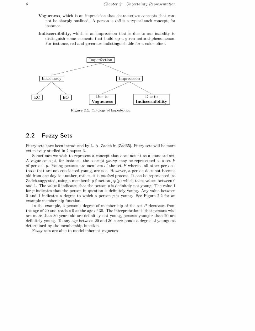
Figure 2.1 shows the classification of imperfection suggested by Worboys. Thereare two classes of imperfections:
Inaccuracy, which is a description, or a mapping, of some natural phenomenonthat does not agree with reality. There are two kinds of such inaccuracies:
Error of Commission(EC) occurs when an element in the mapping doesnot exist in the real situation. For instance, a map of Sweden thatcontains the city of Paris.
Error of Omission (EO) occurs when the mapping fails to report an ele-ment that does exist in the real situation. For instance, a map of Swedenthat does not contain the city of Stockholm.
Imprecision refers to mappings of some natural phenomenons that are not rep-resented exactly as they appear. In this thesis, we focus on the following twokind of imprecision:
5
6 Chapter 2. Uncertainty Representation
Vagueness, which is an imprecision that characterizes concepts that can-not be sharply outlined. A person is tall is a typical such concept, forinstance.
Indiscernibility, which is an imprecision that is due to our inability todistinguish some elements that build up a given natural phenomenon.For instance, red and green are indistinguishable for a color-blind.
EC EO
Inaccuracy
Due toVagueness
Due toIndiscernibility
Imprecision
Imperfection
Figure 2.1. Ontology of Imperfection
2.2 Fuzzy Sets
Fuzzy sets have been introduced by L. A. Zadeh in [Zad65]. Fuzzy sets will be moreextensively studied in Chapter 3.
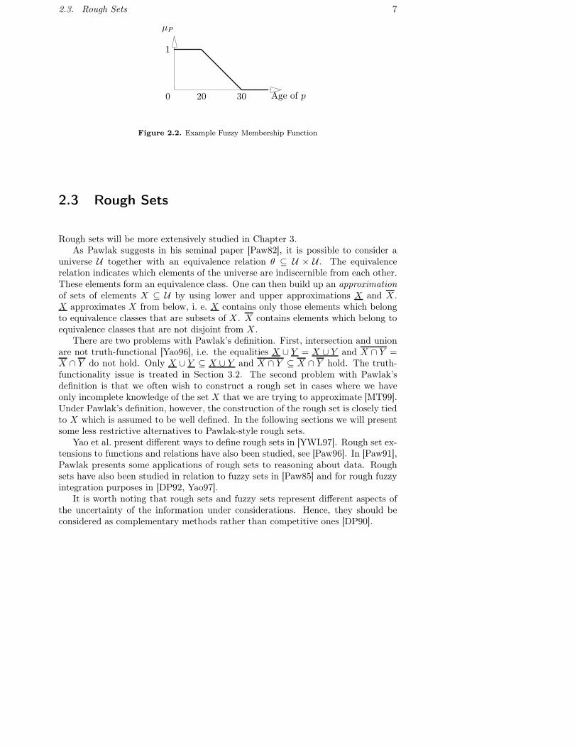
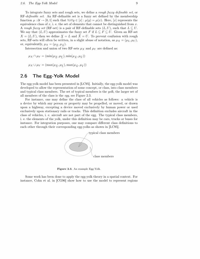
Sometimes we wish to represent a concept that does not fit as a standard set.A vague concept, for instance, the concept young, may be represented as a set Pof persons p. Young persons are members of the set P whereas all other persons,those that are not considered young, are not. However, a person does not becomeold from one day to another, rather, it is gradual process. It can be represented, asZadeh suggested, using a membership function µP (p) which takes values between 0and 1. The value 0 indicates that the person p is definitely not young. The value 1for p indicates that the person in question is definitely young. Any value between0 and 1 indicates a degree to which a person p is young. See Figure 2.2 for anexample membership function.
In the example, a person’s degree of membership of the set P decreases fromthe age of 20 and reaches 0 at the age of 30. The interpretation is that persons whoare more than 30 years old are definitely not young, persons younger than 20 aredefinitely young. To any age between 20 and 30 corresponds a degree of youngnessdetermined by the membership function.
Fuzzy sets are able to model inherent vagueness.
2.3. Rough Sets 7
0 20 30 Age of p
1
µP
Figure 2.2. Example Fuzzy Membership Function
2.3 Rough Sets
Rough sets will be more extensively studied in Chapter 3.As Pawlak suggests in his seminal paper [Paw82], it is possible to consider a
universe U together with an equivalence relation θ ⊆ U × U . The equivalencerelation indicates which elements of the universe are indiscernible from each other.These elements form an equivalence class. One can then build up an approximationof sets of elements X ⊆ U by using lower and upper approximations X and X .X approximates X from below, i. e. X contains only those elements which belongto equivalence classes that are subsets of X . X contains elements which belong toequivalence classes that are not disjoint from X .
There are two problems with Pawlak’s definition. First, intersection and unionare not truth-functional [Yao96], i.e. the equalities X ∪ Y = X ∪ Y and X ∩ Y =X ∩ Y do not hold. Only X ∪ Y ⊆ X ∪ Y and X ∩ Y ⊆ X ∩ Y hold. The truth-functionality issue is treated in Section 3.2. The second problem with Pawlak’sdefinition is that we often wish to construct a rough set in cases where we haveonly incomplete knowledge of the set X that we are trying to approximate [MT99].Under Pawlak’s definition, however, the construction of the rough set is closely tiedto X which is assumed to be well defined. In the following sections we will presentsome less restrictive alternatives to Pawlak-style rough sets.
Yao et al. present different ways to define rough sets in [YWL97]. Rough set ex-tensions to functions and relations have also been studied, see [Paw96]. In [Paw91],Pawlak presents some applications of rough sets to reasoning about data. Roughsets have also been studied in relation to fuzzy sets in [Paw85] and for rough fuzzyintegration purposes in [DP92, Yao97].
It is worth noting that rough sets and fuzzy sets represent different aspects ofthe uncertainty of the information under considerations. Hence, they should beconsidered as complementary methods rather than competitive ones [DP90].
8 Chapter 2. Uncertainty Representation
2.4 Marek’s Model
In [MT99], Marek et al. have introduced a less restrictive rough set model basedon Iwinski’s work [Iwi87].
As for Pawlak-style rough sets, Marek’s model requires an approximation space(U , θ) where θ is an equivalence relation imposing a granularity on a finite universeU . A definable set in this universe is a union of equivalence classes, i. e. setscontaining indiscernible elements. A rough set, in the sense of Marek, is a pair ofdefinable sets (L, U) such that L ⊆ U . Such a construction is an approximationof any set A such that L ⊆ A ⊆ U . Given X = (L, U), we define the lowerapproximation of X , denoted X˜ , and upper approximation of X , denoted X, asX˜ = L and X = U respectively.
Obviously then, for a certain element x ∈ U , if x /∈ U , then x /∈ X , if x ∈ L,then x ∈ X and, finally, if x ∈ U \ L (the area of uncertainty), then we are not sureif x belongs to X or not.
The difference between the above and Pawlak’s definition of a rough set is thatPawlak defines a rough set as an approximation to a specific set, say X . Also, thisrough set is a pair (X, X), where X (resp. X) is the ‘maximal’ (resp. ‘minimal’)definable set that obeys X ⊆ X , respectively X ⊆ X .
Rough sets as defined here are a modification of Pawlak-style rough sets. Theyhave truth-functional intersection and union operators as shown below.
(L, U) ∩ (L′, U ′) = (L ∩ L′, U ∩ U ′)
(L, U) ∪ (L′, U ′) = (L ∪ L′, U ∪ U ′)
Where X = (L, U) and Y = (L′, U ′).If (L, U) approximates a given crisp set A, and (L′, U ′) approximates a given
crisp set B, then (L∩L′, U∩U ′) approximates A∩B and (L∪L′, U∪U ′) approximatesA ∪ B. The approximation operations may be defined as shown below.
X ∩ Y˜
= X˜ ∩ Y˜ and X ∪ Y˜
= X˜ ∪ Y˜X ∩ Y = X ∩ Y and X ∪ Y = X ∪ Y
2.5 Rough Fuzzy Extension of Marek’s Model
In [AKO03], we have introduced a particular rough-fuzzy hybrid model based onMarek’s work.
Dubois and Prade [DP92] have proposed the concept of rough fuzzy set, whichis a Pawlak-style rough approximation of a fuzzy set. The following definition isbased on their work, modified to correspond to the definition of Marek-style roughsets.
2.6. The Egg-Yolk Model 9
To integrate fuzzy sets and rough sets, we define a rough fuzzy definable set, orRF-definable set. An RF-definable set is a fuzzy set defined by the membershipfunction µ : U → [0, 1] such that ∀x∀y ∈ [x] : µ(y) = µ(x). Here, [x] represents theequivalence class of x, i. e. the set of elements that cannot be distinguished from x.A rough fuzzy set (RF-set) is a pair of RF-definable sets (L, U), such that L ⊆ U .We say that (L, U) approximates the fuzzy set F if L ⊆ F ⊆ U . Given an RF-setX = (L, U), then we define X˜ = L and X = U . To prevent confusion with roughsets, RF-sets will often be written, in a slight abuse of notation, as µX = (µL, µU ),or, equivalently, µX = (µX˜ , µ eX).
Intersection and union of two RF-sets µX and µY are defined as:
µX ∩ µY = (min(µX˜ , µY˜), min(µ eX , µeY ))
µX ∪ µY = (max(µX˜ , µY˜), max(µ eX , µeY ))
2.6 The Egg-Yolk Model
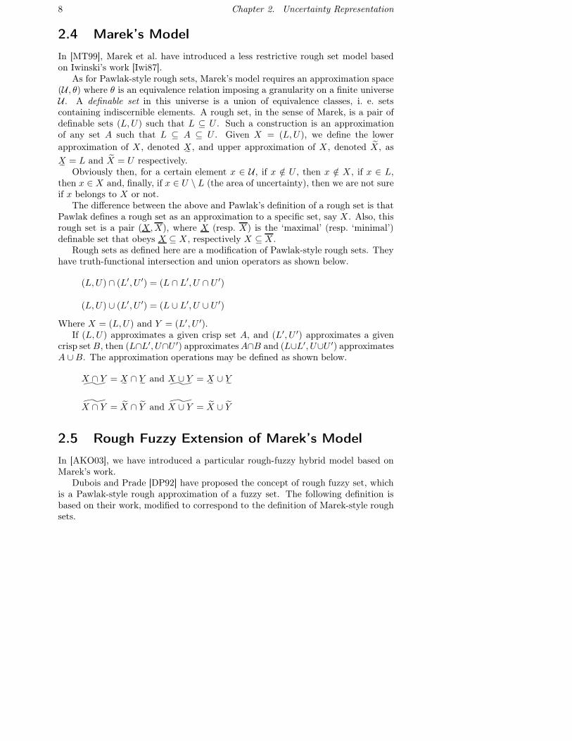
The egg-yolk model has been presented in [LC95]. Initially, the egg-yolk model wasdeveloped to allow the representation of some concept, or class, into class membersand typical class members. The set of typical members is the yolk, the larger set ofall members of the class is the egg, see Figure 2.3.
For instance, one may define the class of all vehicles as follows: a vehicle isa device by which any person or property may be propelled, or moved, or drawnupon a highway, excepting a device moved exclusively by human power or usedexclusively upon stationary rails or tracks. This definition excludes aircraft in theclass of vehicles, i. e. aircraft are not part of the egg. The typical class members,i. e. the elements of the yolk, under this definition may be cars, trucks or buses forinstance. For integration purposes, one may compare different class definitions toeach other through their corresponding egg-yolks as shown in [LC95].
typical class members
class members
Figure 2.3. An example Egg-Yolk.
Some work has been done to apply the egg-yolk theory in a spatial context. Forinstance, Cohn et al. in [CG96] show how to use the model to represent regions
10 Chapter 2. Uncertainty Representation
with indeterminate boundaries. Ways to represent relations between regions withindeterminate boundaries using the egg-yolk model have been presented in [RS01].
Some studies comparing the rough set and the egg-yolk theories have beenpresented in [BP01].
2.7 Other ModelsInterval set is an extension of standard set theory that may be used for uncertainreasoning. There are several equivalent definitions of interval sets [Iwi87, MT99,Yao96]. We pick the one presented by Yao. Let U be a finite set, called the universe,and 2U its power set. A subset of 2U of the form [I, I ′] = {X ∈ 2U |I ⊆ X ⊆ I ′}is called an interval set. The set I is called the lower bound of the interval set andthe set I ′ the upper bound.
In [SW98], Stell et al. have specified a model that is closely related to roughsets called vague regions. A vague region is also defined over a partition. Let Rbe a set of elements considered as basic regions. The basic regions may be cellsin a subdivision of physical space or pixels. For a given partition A of R definedthrough the function σ : R → A, one can define a vague region with the functionv : A → {in, maybe, out}. The set of basic regions definitely included in the vagueregions is defined as:
lower(v) = {r ∈ R|v σ r = in}
The set of basic regions that is possibly included in the vague regions is defined as:
upper(v) = {r ∈ R|v σ r = out}
As stated in [SW98], a vague region can be thought of as standing for any regionthat lies between the union of the elements of lower(v) and the union of the elementsof upper(v).
2.8 ConclusionWe have presented different methods that can be used to represent uncertaintywhen mapping natural phenomena into the computer.
In Section 2.5 we have presented our extension [AKO03] of Marek’s model tosupport vagueness. It turns out that if we define a partial order on Marek-stylerough sets presented in Section 2.4, then Marek-style rough sets can be comparedto Pawlak-style rough sets. To do so, we define the knowledge ordering �kn [MT99]on pairs of definable sets (L, U) as:
(L1, U1) �kn (L2, U2) if L1 ⊆ L2 and L1 ⊆ L2
In this case, if (L, U) approximates the set X , then, (L, U) �kn (X, X). The latterstatement means that Pawlak-style rough sets are �kn-maximal Marek-style rough

2.8. Conclusion 11
sets. As a consequence, Pawlak-style rough sets may be better approximations thanMarek-style rough sets. We therefore focus on Pawlak-style rough sets and theirintegration with fuzzy sets in the remainder of this thesis.

12
Chapter 3
Indiscernibility and Vagueness
We study the theory of rough sets and the theory of fuzzy sets and their integrationinto a unified model called rough fuzzy sets.
Section 3.1 presents approximation of sets which is the theoretical basis of roughsets. Section 3.2 investigates the truth-functionality issue related to the utilizationof rough sets. Section 3.4 shows how to approximate fuzzy sets.
3.1 Approximation of SetsRough sets were first introduced by Pawlak [Paw82] and are based on approximationspaces. An approximation space is a pair A = (U , θ). Here, θ is an equivalencerelation, also called indiscernibility relation, imposing a granularity on the universeU such that θ ⊆ U × U . Furthermore, we assume U to be finite. For x ∈ U , let[x]θ be the equivalence class containing x, i. e. [x]θ = {y | y θ x}. The element x isreferred to as the class representative of the equivalence class [x]θ. The quotientset U/θ is the set of all equivalence classes.
Given an arbitrary set X ⊆ U , we wish to describe X in terms of elements orgranules of U/θ. Pawlak proposed the use of lower and upper approximations of aset X , denoted Aθ(X) and Aθ(X), respectively. Lower and upper approximationsare defined as:
Aθ(X) = {x ∈ U | [x]θ ⊆ X},
Aθ(X) = {x ∈ U | [x]θ ∩ X = ∅}.
The semantics of the approximations of sets may be defined as follows:
• elements of the universe that belong to Aθ(X) are those elements that surelybelong to the set X ,
• elements that belong to Aθ(X) possibly belong to the set X ,
13
14 Chapter 3. Indiscernibility and Vagueness
• elements that belong to U \ Aθ(X) are elements of the universe that surelydo not belong to the set X .
Hence, the uncertainty lies in Aθ(X)\Aθ(X) which is also called area of uncertainty.Elements of the area of uncertainty may, or may not, belong to X .
The approximation operators can also be considered using membership func-tions. It is possible to define a rough set membership function as presented in [Paw96].The rough membership function µX associates to an element x ∈ U a value between0 and 1 as follows:
µX(x) =card(X ∩ [x]θ)
card([x]θ)
This way,
• µX(x) = 1 iff x ∈ Aθ(X),
• µX(x) = 0 iff x ∈ Aθ(X) and
• 0 < µX(x) < 1 iff x ∈ Aθ(X) \ Aθ(X).
For any sets X, Y ⊆ U , given A = (U , θ), the following properties of approxim-ations hold:
Aθ(X) ⊆ X ⊆ Aθ(X) (3.1)
Aθ(X ∩ Y ) = Aθ(X) ∩ Aθ(Y ) (3.2)
Aθ(X ∩ Y ) ⊆ Aθ(X) ∩ Aθ(Y ) (3.3)
Aθ(X ∪ Y ) ⊇ Aθ(X) ∪ Aθ(Y ) (3.4)
Aθ(X ∪ Y ) = Aθ(X) ∪ Aθ(Y ) (3.5)
Aθ(X \ Y ) = Aθ(X) \ Aθ(Y ) (3.6)
Aθ(X \ Y ) ⊆ Aθ(X) \ Aθ(Y ) (3.7)
X ⊆ Y =⇒ Aθ(X) ⊆ Aθ(Y ) (3.8)
X ⊆ Y =⇒ Aθ(X) ⊆ Aθ(Y ) (3.9)
Proofs of the properties above can be found in [Paw91].Rough sets are defined using lower and upper approximations. Let ∼ be an
equivalence relation defined as:
∀X, Y ⊆ U , X ∼ Y if Aθ(X) = Aθ(Y ) and Aθ(X) = Aθ(Y )
then, ∼ is an equivalence relation on the set of subsets of U , i. e. the power set 2U .The equivalence classes of the equivalence relation ∼ are rough sets. The set of all
3.2. Truth Functionality and Rough Sets 15
rough sets in the approximation space (U , θ), denoted Rθ(U), is the quotient set2U/ ∼.
A rough set R ∈ Rθ(U) is uniquely determined by the pair (Aθ(X),Aθ(X)).Here the set X is called the representative of the rough set R. The representativeof a rough set is the set that is being approximated in the approximation space(U , θ).
A rough set (Aθ(X),Aθ(X)) is said to be crisp, or definable, if Aθ(X)\Aθ(X) =∅. It is said to be rough, or not definable, otherwise.
A set Y ⊆ U is member of the rough set R = (Aθ(X),Aθ(X)), denoted Y ∈ R,if Aθ(Y ) = Aθ(X) and Aθ(Y ) = Aθ(X), hence, any member of R can be used as arepresentative for the rough set R as stated by the following equality:
R = (Aθ(X),Aθ(X)) = (Aθ(Y ),Aθ(Y ))
[x]θ ⊆ X
[x]θ ∩ X = ∅X
Y
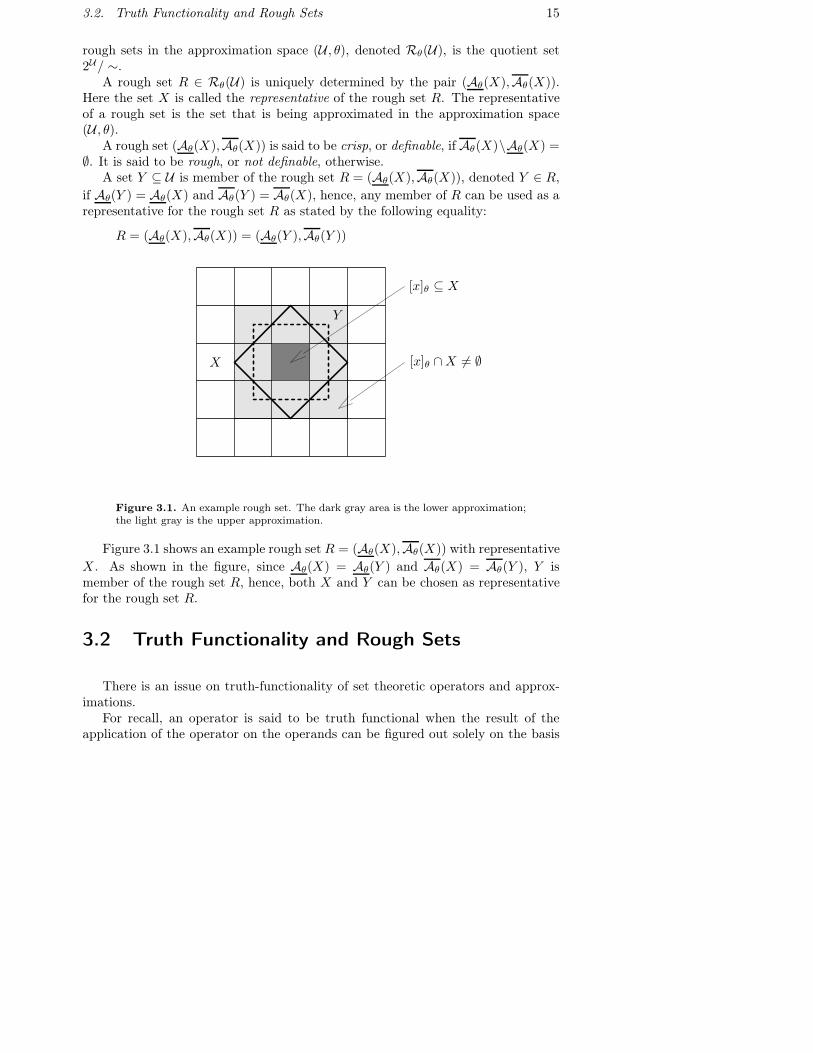
Figure 3.1. An example rough set. The dark gray area is the lower approximation;the light gray is the upper approximation.
Figure 3.1 shows an example rough set R = (Aθ(X),Aθ(X)) with representativeX . As shown in the figure, since Aθ(X) = Aθ(Y ) and Aθ(X) = Aθ(Y ), Y ismember of the rough set R, hence, both X and Y can be chosen as representativefor the rough set R.
3.2 Truth Functionality and Rough Sets
There is an issue on truth-functionality of set theoretic operators and approx-imations.
For recall, an operator is said to be truth functional when the result of theapplication of the operator on the operands can be figured out solely on the basis
16 Chapter 3. Indiscernibility and Vagueness
of the operands. This is not the case for intersection and union of upper and lowerapproximations.
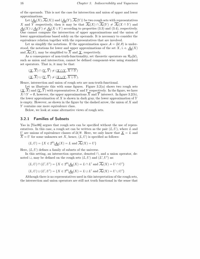
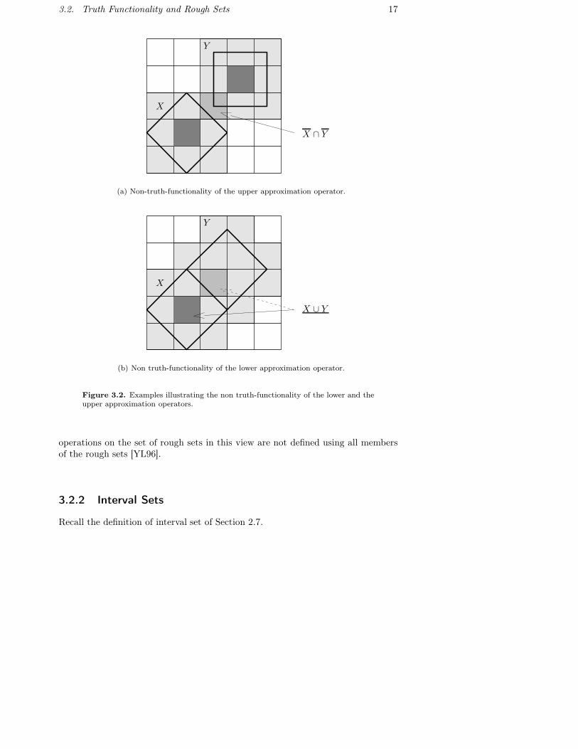
Let (Aθ(X),Aθ(X)) and (Aθ(Y ),Aθ(Y )) be two rough sets with representativesX and Y respectively, then it may be that Aθ(X) ∩ Aθ(Y ) = Aθ(X ∩ Y ) andAθ(X) ∪Aθ(Y ) = Aθ(X ∪ Y ) according to properties (3.3) and (3.4), respectively.One cannot compute the intersection of upper approximations and the union oflower approximations based solely on the operands. It is necessary to consider theequivalence relation together with the representatives that are involved.
Let us simplify the notations. If the approximation space A = (U , θ) is under-stood, the notations for lower and upper approximations of the set X , i. e. Aθ(X)and Aθ(X), may be simplified to X and X , respectively.
As a consequence of non-truth-functionality, set theoretic operators on Rθ(U),such as union and intersection, cannot be defined component-wise using standardset operators. That is, it may be that:
(X, X) ∩ (Y , Y ) = (X ∩ Y , X ∩ Y )
(X, X) ∪ (Y , Y ) = (X ∪ Y , X ∪ Y ).
Hence, intersection and union of rough sets are non-truth-functional.Let us illustrate this with some figures. Figure 3.2(a) shows two rough sets
(X, X) and (Y , Y ) with representatives X and Y respectively. In the figure, we haveX ∩Y = ∅, however, the upper approximations X and Y intersect. In figure 3.2(b),the lower approximation of X is shown in dark gray, the lower approximation of Yis empty. However, as shown in the figure by the dashed arrow, the union of X andY contains one more equivalence class.
Below, we look at some alternative views of rough sets.
3.2.1 Families of SubsetsYao in [Yao96] argues that rough sets can be specified without the use of repres-entatives. In this case, a rough set can be written as the pair (L, U), where L andU are unions of equivalence classes of U/θ. Here, we only know that X = L andX = U for some unknown set X , hence, (L, U) is specified as follows:
(L, U) = {X ∈ 2U |Aθ(X) = L and Aθ(X) = U}
Here, (L, U) defines a family of subsets of the universe.In this setting, an intersection operator, denoted �, and a union operator, de-
noted �, may be defined on the rough sets (L, U) and (L′, U ′) as:
(L, U) � (L′, U ′) = {X ∈ 2U |Aθ(X) = L ∩ L′ and Aθ(X) = U ∩ U ′}
(L, U) � (L′, U ′) = {X ∈ 2U |Aθ(X) = L ∪ L′ and Aθ(X) = U ∪ U ′}Although there is no representatives used in this interpretation of the rough sets,
the intersection and union operators are still not truth functional in the sense that
3.2. Truth Functionality and Rough Sets 17
X ∩ Y
X
Y
(a) Non-truth-functionality of the upper approximation operator.
X ∪ Y
X
Y
(b) Non truth-functionality of the lower approximation operator.
Figure 3.2. Examples illustrating the non truth-functionality of the lower and theupper approximation operators.
operations on the set of rough sets in this view are not defined using all membersof the rough sets [YL96].
3.2.2 Interval Sets
Recall the definition of interval set of Section 2.7.
18 Chapter 3. Indiscernibility and Vagueness
For two interval sets I = [I, I ′] and J = [J, J ′], the following truth-functionaloperations on interval sets are defined:
I � J = [I ∩ J, I ′ ∩ J ′] (3.10)I � J = [I ∪ J, I ′ ∪ J ′] (3.11)I \ J = [I − J ′, I ′ − J ] (3.12)
According to Yao [Yao93], rough sets provide a way to construct interval sets.Provided a finite universe U , an equivalence relation θ, and a set X we wish toapproximate, an interval set can be constructed as
[Aθ(X),Aθ(X)
].
The reverse process, however, is not straightforward. That is, given a finiteuniverse U and an interval set [I, I ′] where I, I ′ ⊆ 2U , there might be more thanone approximation space A = (U , θ) such that I = Aθ(X) and I ′ = Aθ(X) for someX . Hence, we do not have enough information to reconstruct the initial rough set.
3.2.3 Restriction of Approximations
Here, we present an alternative based on restriction of approximations. Instead ofconsidering all subsets of the universe 2U in the approximation space (U , θ), onlysome particular subsets R ⊂ 2U are considered. The idea is to choose R in sucha way that truth-functionality of the intersection and union operators hold, i. e.∀X, Y ∈ R, Aθ(X ∪ Y ) = Aθ(X) ∪Aθ(Y ) and Aθ(X ∩ Y ) = Aθ(X)∪Aθ(Y ) hold.To simplify the terminology, in this case, we say that R is a set of truth-functionalrepresentatives.
Below, we present a way to achieve this as described in [Yao93]. The methodis based on a uniform set of representatives that has been introduced by Gehrke etal. in [GW92]. We also extend this method later to fit our need to represent spatialuncertainty.
Uniform Set of Representatives
For recall, a set of class representatives of a quotient set is a set that containsexactly one element from each equivalence class of the quotient set.
For any equivalence class E ∈ U/θ with at least two elements, we define a set AE
such that ∅ ⊂ AE ⊂ E and we let A =⋃
E∈U/θ AE . We call A the template set. Ifthe equivalence class E contains exactly one element we set AE = ∅. Furthermore,we let RA denote the set defined as:
RA = {XA|XA = X ∪ (X ∩ A), ∀X ⊆ U}
The set RA is a set of class representatives of 2U/ ∼. This is the case sinceXA = YA =⇒ XA ∼ YA as stated in the following lemma.
Lemma 3.1. For any pair of elements XA, YA ∈ RA, if XA = YA then XA ∼ YA.
3.2. Truth Functionality and Rough Sets 19
Proof.
XA = YA =⇒ X ∪ (X ∩ A) = Y ∪ (Y ∩ A) =⇒
X = Y∨
(X ∩ A) = (Y ∩ A)
because of the construction of A. Thus, either X = Y which implies XA = YA, or,(X ∩A) = (Y ∩A). For the latter case to be true it must be the case that at leastone element of A belongs to X but does not belong to Y , or, conversely, at leastone element of A belongs to Y and does not belong to X . In both cases we havethat XA = YA. Hence, XA and YA cannot belong to the same equivalence class of2U/ ∼, i. e. XA ∼ YA.
As a consequence, to each subset X ⊆ U , given a fixed set A defined as above,corresponds a unique class representative XA ∈ RA such that X ∼ XA.
Now, let us look at the truth-functionality issue.
Lemma 3.2. Let A be a template set defined as above, then ∀XA, YA ∈ RA, thefollowing equalities hold:
Aθ(XA ∪ YA) = Aθ(XA) ∪ Aθ(YA) (3.13)
Aθ(XA ∩ YA) = Aθ(XA) ∩ Aθ(YA) (3.14)
Proof. ∀E ∈ U/θ and X ⊆ U we define XE = X ∩ E. Since X =⋃
E∈U/θ XE
and⋂
E∈U/θ XE = ∅, it suffices to show that both equalities 3.13 and 3.14 hold for(XE)A and (YE)A, that is:
(XE)A ∪ (YE)A = (XE)A ∪ (YE)A
(XE)A ∩ (YE)A = (XE)A ∩ (YE)A
In the case when E ⊆ X or E ⊆ Y , either (XE)A = E or (XE)A = E, in bothcases we have that:
(XE)A ∪ (YE)A = (XE)A ∪ (YE)A = E
(XE)A ∩ (YE)A = (XE)A ∩ (YE)A = E
Let us consider the case when E intersects both X and Y and E ⊂ X and E ⊂ Y ,then, XE = YE = ∅ and XE ∩ AE = YE ∩AE = AE , hence, (XE)A = (YE)A = AE
and both equalities 3.13 and 3.14 hold.
Hence, if we restrict our domain to the set RA, then, intersection and union ofapproximations are truth-functional. As a consequence, intersection and union

20 Chapter 3. Indiscernibility and Vagueness
operations can be defined component-wise on the rough sets (X, X) and (Y , Y )when X, Y ∈ RA as follows:
(X, X) ∩ (Y , Y ) = (X ∩ Y , X ∩ Y )
(X, X) ∪ (Y , Y ) = (X ∪ Y , X ∪ Y )
Restricted approximations may be used as described below.Suppose we wish to approximate sets X, Y ⊆ U in an approximation space
(U , θ). We first define a template set A which will impose the representatives ofRA that are to be used. Next, we substitute sets X and Y by their correspondingrepresentatives XA and YA in RA, i. e. X ∼ XA and Y ∼ YA. In any subsequentoperation, XA and YA are used instead of X and Y .
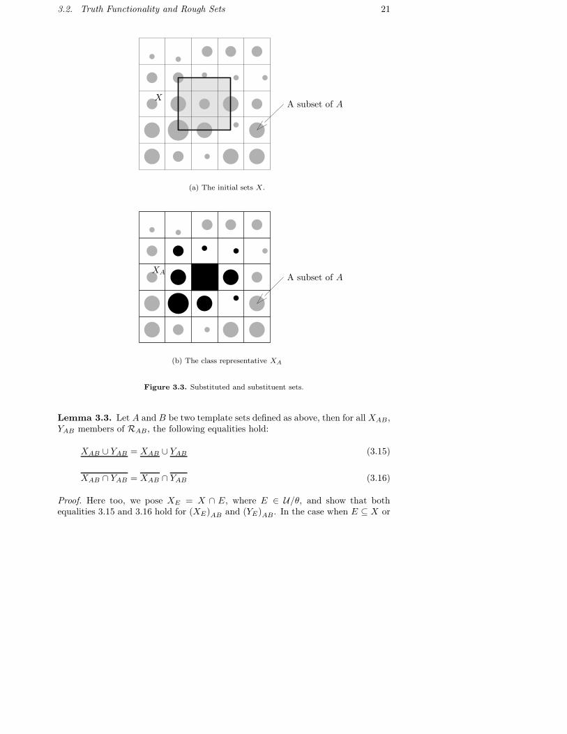
Substituting arbitrary subsets X by their corresponding uniform representativesXA is admissible with respect to a given equivalence relation ∼, however, sometimeswe wish the substituent of a set X to satisfy an additional condition beside theequivalence X ∼ XA. An example of such a condition may be that the substitutedset X and the substituent set XA do not differ in too many elements, i. e. theyhave as many elements in common as possible. Obviously, this can be achieved ifwe succeed in growing the size of the set of truth-functional representatives R.
Let us look at the example of Figure 3.3. In the figure, the template set Ais shown as light gray filled circles. Figure 3.3(a) shows the set X , shown as agray filled square, that is to be substituted. The class representative XA that willsubstitute X is shown in Figure 3.3(b) as a set of black filled circles and a black filledsquare. The latter example shows that a class representative XA of a substitutedset X can differ in relatively many elements. In fact, it may happen that they donot have any elements in common even though X ∼ XA.
Below, we introduce a modified version of uniform set of representatives in whichwe do not allow substituted sets and their corresponding substituents to differ inmore than 2 · |U/θ| elements.
Extended Uniform Set of Representatives
Let A and B be two sets of class representatives from which we eliminate elementsthat are class representatives of singleton sets of U/θ. Moreover, sets A and B aredefined such that A ∩ B = ∅. Let RAB denote the set defined as:
RAB ={XAB|XAB =
(X ∪ (X ∩ A)
)\
((X \ X) ∩ B
), ∀X ⊆ U
}
Here too, sets A and B are called template sets.A set XAB defined as above may substitute the set X since X ∼ XAB. Moreover,
by its construction, if an equivalence class E ∈ U/θ intersects X such that E ⊂ X ,then, X ∩ E and XAB ∩ E may differ at most at two elements. That is, X ∩ Emight not contain A∩E but might contain B∩E, XAB, on the other hand, containsA ∩ E but does not contain B ∩ E. As a consequence, the substituted set and thesubstituent differ at most at 2 · |U/θ| elements.
3.2. Truth Functionality and Rough Sets 21
A subset of AX
(a) The initial sets X.
A subset of AXA
(b) The class representative XA
Figure 3.3. Substituted and substituent sets.
Lemma 3.3. Let A and B be two template sets defined as above, then for all XAB,YAB members of RAB, the following equalities hold:
XAB ∪ YAB = XAB ∪ YAB (3.15)
XAB ∩ YAB = XAB ∩ YAB (3.16)
Proof. Here too, we pose XE = X ∩ E, where E ∈ U/θ, and show that bothequalities 3.15 and 3.16 hold for (XE)AB and (YE)AB. In the case when E ⊆ X or

22 Chapter 3. Indiscernibility and Vagueness
E ⊆ Y , either (XE)AB = E or (XE)AB = E, in both cases we have that:
(XE)AB ∪ (YE)AB = (XE)AB ∪ (YE)AB = E
(XE)AB ∩ (YE)AB = (XE)AB ∩ (YE)AB = E
Let us consider the case when E intersects both X and Y and E ⊂ X and E ⊂ Y .Then, by their construction, (XE)AB and (YE)AB have an element in commonwhich is (A ∩ E) and an element (B ∩ E) which is missing from both (XE)AB and(YE)AB. Hence, both equalities 3.15 and 3.16 hold.
Hence, intersection and union of approximations of elements of RAB are truth-functional.
An example element XAB of RAB is shown in Figure 3.4. In the figure, ablack dot represents an element of the template set A and a gray dot represents anelement of the template set B.
XAB
Figure 3.4. An example element XAB
As previously, if we restrict our domain to the set RAB , then, for rough sets(X, X) and (Y , Y ) where the representatives are such that X, Y ∈ RAB , we havethat:
(X, X) ∩ (Y , Y ) = (X ∩ Y , X ∩ Y )
(X, X) ∪ (Y , Y ) = (X ∪ Y , X ∪ Y )
There is an interesting issue concerning the set of truth-functional represent-atives RAB : the complement of an element of RAB is not in RAB . In fact, thecomplement of an element XAB in U , i. e. (U \XAB), is an element of RBA. Hence,sets A and B play a symmetric role.
3.4. Rough Fuzzy Sets 23
3.3 Fuzzy SetsLet U be a universe of discourse. A standard set A in U may be defined as a set ofordered pairs A = {(x, IA(x))|x ∈ U}, where IA(x) ∈ {0, 1} is an indicator function.For a given data point x, IA(x) indicates the membership of x in the set A, 0 for xnon-member of the set A and 1 for x member of the set A.
L. A. Zadeh has introduced fuzzy sets in [Zad65]. In a fuzzy set it is possible torepresent the degree of membership of a data point to a given set by a value rangingfrom 0 to 1: a fuzzy set A in U is a set of ordered pairs A = {(x, µA(x))|x ∈ U},defined by a membership function 0 ≤ µA(x) ≤ 1.
Basic set operations extend to fuzzy sets. Let A and B be fuzzy sets defined asA = {(x, µA(x))|x ∈ U} and B = {(x, µB(x))|x ∈ U}. The union and intersectionof fuzzy sets A and B are commonly defined as:
A ∪ B = {(x, µA∪B(x))|x ∈ U}, where µA∪B(x) = max(µA(x), µB(x)),
A ∩ B = {(x, µA∩B(x))|x ∈ U}, where µA∩B(x) = min(µA(x), µB(x)).
The complement of a fuzzy set A = {(x, µA(x))|x ∈ U} in U , denoted ¬A, is definedas ¬A = {(x, µ¬A(x))|x ∈ U}, where µ¬A(x) = 1 − µA(x).
The support of a fuzzy set A is the crisp set containing all non-zero membersof A. The support of a set A is denoted Support(A). An element x belongs toSupport(A) if µA(x) > 0.
According to [Yao97], it may be desirable to explicitly establish a connectionbetween fuzzy sets and crisp sets. In this case one might use instead anotherrepresentation of fuzzy sets that is based on crisp sets. Formally, given α ∈ [0, 1],an α-cut or α-level set, of a fuzzy set A is defined as:
Aα = {x ∈ U|µA(x) ≥ α},
a strong α-cut is defined as:
Aα+ = {x ∈ U|µA(x) > α}.
Fuzzy sets can be reconstructed from their α-cuts, i. e. it is possible to retrieve themembership function µA based solely on the α-level sets Aα:
µA(x) = sup{α|x ∈ Aα}
3.4 Rough Fuzzy SetsDubois and Prade [DP92] have proposed the concept of rough fuzzy set, which is arough approximation of a fuzzy set. Rough fuzzy sets are based on approximationspaces A = (U , θ). Let E = [x]θ ∈ U/θ, we wish to approximate a fuzzy setX ⊆ U in the approximation space A. The lower and upper approximations Aθ(X)
24 Chapter 3. Indiscernibility and Vagueness
and Aθ(X) of a fuzzy set X are fuzzy sets of U/θ with membership functionsµAθ(X), µAθ(X) : U/θ → [0, 1]. The membership functions of the lower and upperapproximations of X are defined respectively as:
µAθ(X)(E) = inf{µX(x)|E = [x]θ}
µAθ(X)(E) = sup{µX(x)|E = [x]θ}
Given a fuzzy set X , the pair (µAθ(X), µAθ(X)) is called a rough fuzzy set. Onecan also extend the membership functions µAθ(X) and µAθ(X) to be defined overthe universe U using the extension principle introduced by Zadeh [Zad65]. Thisway, the membership functions are defined as:
µAθ(X), µAθ(X) : U → [0, 1]
µAθ(X)(x) = inf{µX(y)|y ∈ [x]θ}
µAθ(X)(x) = sup{µX(y)|y ∈ [x]θ}Rough fuzzy sets are able to express uncertainty due to indiscernibility as well
as uncertainty due to vagueness.Given an approximation space (U , θ) and fuzzy sets X, Y ⊆ U , ∀E ∈ U/θ
and ∀x ∈ U , the following properties of approximations of rough fuzzy sets may bededuced from the properties of rough sets presented in Section 3.1 (see also [Thi98]):
µAθ(X)(E) ≤ µX(E) ≤ µAθ(X)(E) (3.17)
µAθ(X∩Y )(E) = min(µAθ(X)(E), µAθ(Y )(E)) (3.18)
µAθ(X∩Y )(E) <= min(µAθ(X)(E), µAθ(Y )(E)) (3.19)
µAθ(X∪Y )(E) >= max(µAθ(X)(E), µAθ(Y )(E)) (3.20)
µAθ(X∪Y )(E) = max(µAθ(X)(E), µAθ(Y )(E)) (3.21)
µX(x) ≤ µY (x) =⇒ µAθ(X)(E) ≤ µAθ(Y )(E) (3.22)
µX(x) ≤ µY (x) =⇒ µAθ(X)(E) ≤ µAθ(Y )(E) (3.23)
See [Pol02] for proofs of the properties above.If the approximation space A = (U , θ) is understood, the notations for lower
and upper approximations, µAθ(X) and µAθ(X), of a fuzzy set X , may be simplifiedto µX and µX , respectively.
Intersection and union of rough fuzzy sets are non-truth-functional according toproperties 3.19 and 3.20. However, restriction of approximations of Section 3.2.3also extends to rough-fuzzy sets. Hence, truth-functional intersection and unionoperations may be defined on rough-fuzzy sets as shown below.
The definition of extended uniform set representatives may be adapted to holdfor rough fuzzy sets. This time, we wish to build a set of fuzzy set representatives
3.5. Conclusion 25
FAB such that they support truth-functional intersection and union operations.The fuzzy sets A and B, with membership functions µA and µB respectively, aresuch that Support(A) and Support(B) are two disjoint set of class representativesof U/θ.
We wish to achieve that if X, Y ∈ FAB then the following equalities hold:
µX∩Y (E) = min(µX(E), µY (E))
µX∪Y (E) = max(µX(E), µY (E))
This turns out to hold only if:
∀α ∈ R, Xα, Yα ∈ RAαBα
for some fixed fuzzy sets A and B.
3.5 ConclusionAs seen in this chapter, intersection and union of approximations are non-truth-functional. We point out two main issues caused by non-truth-functionality ofrough sets in our spatial information system.
The first issue is related to unknown set representatives. For instance, assumethat two unknown subsets of the universe X and Y have been approximated insome approximation space. Moreover, the only information at hand is the lowerand upper approximations of the sets in question, i. e. the rough sets (L, U) and(L′, U ′), then we cannot compute the union and intersection of these two roughsets.
The second issue is related to measuring areas of uncertainty. Consider that theelements of the universe are now polygons, representing some spatial information,with an area. In this case, since X ∩ Y ⊆ X ∩ Y , the following inequality holds:
area(X) ∩ area(Y ) ≥ area(X ∩ Y )
Hence, performing intersection of upper approximations leads to overestimating thearea of intersection.
We have shown that it is possible to avoid the truth-functionality issues bychanging representatives. The drawback is, of course, that we do not approximatethe initial set but some substituent. Clearly, this leads to introducing some moreimprecision in the data set.
There is, however, another way we may look at the problem. The extendeduniform set of representatives may be seen as a property. The fact that two setsX and Y belong to RAB, for some disjoint class representatives A and B, makesintersection and union operations on X and Y truth-functional. Hence, given a setof subsets Xi we wish to approximate, we may look for the set of representatives Aand B such that Xi ∈ RAB for all i.

26 Chapter 3. Indiscernibility and Vagueness
Hence, we may be given pairs of upper and lower approximations (Li, Ui) withthe claim that they are the result of some approximations Li = Xi and Ui = Xi
where, for all i, Xi ∈ RAB. In this case, we may combine the pairs of approxima-tions with intersection and union operations. As a consequence, computing area ofpolygons, or cardinality of sets, may be done exactly:
area(Ui) ∩ area(Uj) = area(Ui ∩ Uj)
Chapter 4
Spatial and Attribute Uncertainty
In this chapter we extend the query language by Marek et al. [MT99] in a way thatallows us to represent indiscernibility and vagueness. To represent indiscernibilitywe use rough set theory and to represent vagueness we use fuzzy set theory.
The query language presented in [MT99] is based on the concept of inform-ation system. Our query language, on the other hand, is based on multi-valuedinformation systems.
We first recall the concept of multi-valued information systems, then Section 4.2shows how we extend this concept to support approximation spaces. Section 4.3and 4.4 present a novel approach to perform classifications. Finally, in Section 4.5,we show how to extend our model to support vagueness.
4.1 Multi-valued Information Systems
Let U be a finite set of elements called the universe and AT a non-empty finiteset of attributes a ∈ AT , such that a : U → Va. The set Va is called the rangeof the attribute a. For an element x ∈ U and an attribute a ∈ AT , the pair(x, a(x)) ∈ U × Va indicates that x has the attribute value a(x). The pair (U ,AT )is called an information system [DGO01] and is often referred to as a single-valuedinformation system. In a single-valued information system, attributes a ∈ AT mapelements x ∈ U to a single attribute value v = a(x) in the range Va.
A multi-valued information system is a generalization of the idea of a single-valued information system. In a multi-valued information system, attribute func-tions are allowed to map elements to sets of attribute values [KR96, DGO01](see also [DG00]). More formally, we allow multi-valued attributes a such thata : U → 2Va . A subset a(x) ⊆ Va may also be referred to as an attribute value.
Since a may map x to more than one attribute value at a time we need aninterpretation for a(x) = V . Düntsch et al. in [DGO01] propose the following ones:
27

28 Chapter 4. Spatial and Attribute Uncertainty
(CEX) V is interpreted conjunctively and exhaustively, i. e. all elements of V andonly those elements are attributes of element x. As an example, consider theattribute a, cooperates with, where a(‘Karim’) = {‘Johannes’, ‘Ola’}. In thisinterpretation, ‘Karim’ cooperates with ‘Johannes’ and ‘Ola’ and no one else.
(CNE) V is interpreted conjunctively and non-exhaustively, i. e. all elements of Vand possibly others are attributes of element x. Using the previous example,in this case, ‘Karim’ cooperates with ‘Johannes’ and ‘Ola’ and possibly others.
(DEX) V is interpreted disjunctively and exclusively, i. e. one and only one ele-ment of V is attribute of element x but it is not known which one. Here,‘Karim’ cooperates with ‘Johannes’ or ‘Ola’ but not both.
(DNE) V is interpreted disjunctively and non-exclusively, i. e. at least one elementof V and possibly more are attributes of element x. Finally, in this case,‘Karim’ cooperates with ‘Johannes’ or ‘Ola’ or both.
Subsequently, we consider the CEX interpretation. In this interpretation, theattribute value of an element of the universe may be composed of several attributevalues. For instance, in our previous example where ‘Karim’ cooperates with ‘Jo-hannes’ and ‘Ola’, both values ‘Johannes’ and ‘Ola’ compose the attribute values‘Karim’ cooperates with. On the other hand, a disjunctive interpretations is suit-able to represent the uncertainty in the value that an element of the universe mapsto. For instance, ‘Karim‘ cooperates with ‘Johannes’ or ‘Ola’ but we do not knowwhich one of them.
Now, let us discuss how to relate elements of the universe to their attributevalues.
In a multi-valued information system (U ,AT ), each attribute a ∈ AT implies arelation Ra ⊆ U × Va by setting xRa v ⇔ v ∈ a(x). This way, each element of theinformation system can be associated a description by means of a subset A ⊆ ATof attributes, called the A-description, denoted A(x). The tuple A(x) is defined asA(x) =
∏a∈A a(x) such that A(x) belongs to
∏a∈A 2Va. A tuple A(x) may also be
denoted as 〈V 〉A, where V is the value of A(x), or just 〈V 〉 if there is no risk forconfusion.
A useful operation on tuples is the projection operation. The projection oper-ator, denoted πi, maps the i-th element Vi of a tuple as follows:
2V1 × . . . × 2Vi . . . × 2Vnπi−→ 2Vi
〈V1, . . . , Vi, . . . , Vn〉 �−→ Vi
The projection operator πi may be generalized for convenience to a projectionoperator πB that projects a tuple 〈V 〉 ⊆
∏a∈A 2Va on the attributes of a set of
attributes B such that B ⊆ A.Subsequently, we refer to multi-valued information systems simply as informa-
tion systems, a single-valued information system being a particular case of a multi-valued information system.

4.2. Information Systems and Approximation 29
4.2 Information Systems and ApproximationIn this thesis, we further extend multi-valued information systems (U ,AT ) by in-troducing an equivalence relation ∼a, where ∼a⊆ Va ×Va, on the range Va of eachattribute a ∈ AT . By setting equivalence relations on the attribute values of Va weare able to model indiscernibility of attribute values. The only discernible elementsare the equivalence classes of Va/ ∼a, hence, the name of equivalence classes playalso the role of attribute values. For instance, if the equivalence class blue containsthe attribute values ‘sky blue’ and ‘light blue’, then ‘blue’ is also considered as anattribute value.
In this information system, one cannot distinguish an attribute value V ⊆ Va,instead, the attribute value is approximated in the approximation space (Va,∼a).If an element x of the universe has the attribute value a(x) = V , we say thatthe attribute value of x that is discerned is the rough set (V , V ). Note that eachindividual element of the equivalence classes still remain represented in the inform-ation system. However, some users of the information system may only discern theequivalence classes.
Given an attribute value V ⊆ Va, the set V is the set of attribute values of Va
which certainly belong to V . V is the set of elements which possibly belong to V .The set Va \ V certainly belongs to the complement of V in Va, i. e. certainly doesnot belong to V . This interpretation extends to elements of the universe as shownbelow.
Let x be an element of the universe U such as a(x) = V , then:
• the attribute values of a(x) certainly belong to the attribute values of x. Wesay that a(x) are certain attribute values of x.
• the attribute values of a(x) possibly belong to the attribute values of x. Wesay that a(x) are possible attribute values of x.
• the attribute values of Va\a(x) certainly do not belong to the attribute valuesof x.
Let us classify multi-valued information systems into single-granular informa-tion systems and multi-granular information systems. In a single-granular informa-tion system we restrict elements of the universe to have their attribute values in oneand only one equivalence class, i. e. a(x) = V/ ∼a is a singleton for every elementx and attribute a. We do not have such a restriction in multi-granular informationsystems.
4.2.1 Indiscernibility of Attribute Values
Some attribute values may not be discernible from each other in the sense that theymay have identical upper and lower approximations in the approximation spaces(Va,∼a).

30 Chapter 4. Spatial and Attribute Uncertainty
More formally, two attribute values V, V ′ ⊆ Va are indiscernible from each other,denoted V ≈a V ′, if:
(A∼a(V ) = A∼a(V ′)
) ∧(A∼a(V ) = A∼a(V ′)
)It is easily seen that ≈a is an equivalence relation. The equivalence class of a subsetV ⊆ Va in ≈a is denoted [V ]≈a and is an element of the quotient set 2Va/ ≈a.
Let us look at an example.
Example 4.1. An example spatial information system consists of a set of polygons.Each polygon has a number of properties determined by a multi-valued attributeColors . Hence a given polygon may be characterized by several colors. The follow-ing set of attribute values, denoted Vc, will be considered: lime green (lg), yellowgreen (yg), medium sea green (mg), sky blue (sb), light blue (lb), slate gray (sg),dark gray (dg) and white. For obvious reasons we impose the equivalence relation∼ on the set of attribute values as:
Vc/ ∼={{lg, yg, mg}︸ ︷︷ ︸
green
, {sb, lb}︸ ︷︷ ︸blue
, {sg, dg}︸ ︷︷ ︸gray
, {white}}
As shown above, the equivalence classes of our example are named ‘green’, ‘blue’,‘gray’ and ‘white’. In this information system, only the equivalence classes repres-enting the colors ‘green’, ‘blue’, ‘gray’ and ‘white’ are discernible.
Now, consider a polygon pi with the attribute value Colors (pi) = {lg, mg} =V1, the lower approximation V1 in empty and V1 = green, hence, V1 is not definablein our example approximation space. However, it can be approximated using therough set (∅, green). Hence, we can only state that the attribute values ‘lime green’,‘yellow green’ and ‘medium sea green’ are possibly attribute values of pi accordingto the interpretation of rough sets.
Assume now that there is a second polygon pj where Colors (pj) = {yg, mg} =V2. Although V1 and V2 are different sets in the approximation space at hand, theattribute values V1 and V2 are indiscernible since the following hold:
∅ = V1 = V2 � V1 = V2 = green
As a consequence, polygons pi and pj cannot be discerned from each other by meansof the attribute Colors in this example information system.�
Below, we state this more formally.
4.2.2 Indiscernibility of Elements of the UniverseNow that we have defined an equivalence relation on the range of the attributes ofAT we formally show how to induce an equivalence relation on the elements of theuniverse U .

4.2. Information Systems and Approximation 31
Two elements x, y ∈ U may have equivalent attribute values a(x) and a(y), i. e.a(x) ≈a a(y), in which case x and y are indiscernible from each other by means ofthe attribute a. This situation will be denoted xθay. Formally, xθay is defined as:
xθay if(A∼a(a(x)) = A∼a(a(y))
) ∧(A∼a(a(x)) = A∼a(a(y))
),
or, equivalently,
xθay if a(x) ≈a a(y)
In case each attribute a in AT is considered in its approximation space (Va,∼a),the equivalence relation ≈a extends straightforwardly to the composed equivalencerelation ≈A. This is done by combining ≈a and by using the projection operationπ. Let 〈U〉 and 〈V 〉 be two tuples of
∏a∈A 2Va, then the equivalence relation ≈A
is defined as:
〈U〉 ≈A 〈V 〉 if∧a∈A
(πa(〈U〉) ≈a πa(〈V 〉)
)
In this case, the equivalence class of 〈V 〉 in ≈A is a subset of∏
a∈A 2Va and isdenoted [〈V 〉]≈A .
Furthermore, two elements of U may have equivalent A-descriptions in whichcase they are not discernible from each other by means of their A-descriptions.
Let A ⊆ AT and x, y ∈ U , we define an equivalence relation θA on the elementsx, y ∈ U as:
xθAy if ∀a ∈ A,(A∼a(a(x)) = A∼a(a(y))
) ∧(A∼a(a(x)) = A∼a(a(y))
)
Obviously, θA is an equivalence relation.Again, θA can be rewritten using ≈A as:
xθAy if A(x) ≈A A(y)
Remark
It is worth noting that there is another way to represent an attribute value ordescription A(x) in our information system. As we argued in Section 4.1, a multi-valued information system implies a relation Ra ⊆ U ×Va where xRa v ⇔ v ∈ a(x)which can easily be generalized to hold for tuples A(x). Hence, a description A(x)can also be represented as a set of tuples A(x) ⊆
∏a∈A Va instead of a tuple of
sets, i. e. A(x) ∈∏
a∈A 2Va as presented here.Hence, we may look at some other ways to construct θA. For instance, we may
define θA using equivalence of elements of attribute values. As in [YWL97], wedefine a composite equivalence relation ∼A by combining the elementary equivalence
32 Chapter 4. Spatial and Attribute Uncertainty
relations ∼a. Let A = {a1, . . . , an} and the tuples 〈u1, . . . , un〉 and 〈v1, . . . , vn〉elements of V1 × . . . × Vn. The equivalence relation ∼A is defined as:
〈u1, . . . , un〉 ∼A 〈v1, . . . , vn〉 if∧
ai∈A
(ui ∼ai vi)
This way, θA may equivalently be defined as:
xθAy if(A∼A(A(x)) = A∼A(A(y))
) ∧(A∼A(A(x)) = A∼A(A(y))
)
Or, we may use Pawlak’s rough relation model described in [Paw96]. In thismodel, given two sets Va and Vb, two indiscernibility relations ∼a⊆ Va × Va and∼b⊆ Vb × Vb, we define a new indiscernibility relation by constructing the productof the indiscernibility relations ∼a × ∼b.
Now, let us describe some elements of our information system.Elements of the equivalence classes [x]θA are those elements of the universe of
our information system that cannot be discerned from each other by means of theirA-descriptions. Often though, we are interested in the description of elements bymeans of all attributes of the information system. Thus, considering the whole setof attributes AT , the equivalence classes [x]θAT are those subsets of the universethat cannot be discerned in the information system (U ,AT ).
Subsequently, to simplify the notation, we will use θ to denote θAT when ATis understood.
Moreover, throughout this thesis, for convenience, we assume that the equival-ence classes of U/θ have at least two elements.
4.2.3 Description Language
In the context of an information system we have defined an approximation space inwhich subsets of the universe may be approximated using lower and upper approx-imation operators. Here, we define a language that we will use to query elementsof the universe by means of their descriptions.
To the information system (U ,AT ) we associate a language LAT . The languageis an extension of the one presented in [MT99]. The main difference lies in that inthe language we define here we enable the use of approximate descriptions of theelements of the universe in the query.
Our language consists of terms built by means of functor symbols + (sum), ·(product) and − (negation). The terms of LAT are defined recursively as follows:
• For every attribute a ∈ AT and every attribute value V ⊆ Va, the expressiona = V is a term.
• If s and t are terms then so are s+ t (sum), s · t (product) and −s (negation).

4.2. Information Systems and Approximation 33
Terms of LAT are used to query the information systems (U ,AT ). To allowqueries, we define the value of a term a = V , denoted |a = V |, as:
|a = V | ={x ∈ U
∣∣(A∼a(a(x)) = A∼a(V )) ∧(
A∼a(a(x)) = A∼a(V ))}
The value of a query (or term) t to the information system, i. e. |t|, is said to be theanswer, or result, of a query t. The query value |a = V |, or just query for simplicity,returns elements x of the universe whose attribute values a(x) are approximatelyV , i. e. a(x) ≈a V . We refer to this type of query as approximate query.
The value of a sum, product and negation of terms are interpreted as union,intersection and complement, respectively. Hence, |s + t| = |s| ∪ |t|, |s · t| = |s| ∩ |t|and | − t| = U \ |t|.
Moreover, query may apply to several attributes at a time: |(a = V ) · (b = V ′)|,where V ⊆ Va and V ′ ⊆ Vb, for instance. Such a query can equivalently be writtenas:
|a = V | ∩ |b = V ′| = {x|(a(x) ≈a V ) ∧ (b(x) ≈b V ′)} = |A = 〈V, V ′〉|
where A = {a, b}. To simplify the notation we may use V to denote 〈V 〉 when thereis no confusion. We may then define generalized queries of the form |A = V |, whereV is a tuple of
∏a∈A 2Va , as:
|A = V | ={
x ∈ U∣∣(A∼A(a(x)) = A∼A(V )
) ∧(A∼A(a(x)) = A∼A(V )
)}
Observe that for any A ⊆ AT and V ∈∏
a∈A 2Va , |A = V | is an element of thequotient set U/θA. Hence, by combining queries we should be able to approximatesubsets of the universe U in the approximation space (U , θA).
4.2.4 Queries and ApproximationsGiven an information system (U ,AT ) and an approximation space θA, subsetsX ⊆ U are approximated by means of queries |A = V |.
Let us consider queries with only one attribute a.To each equivalence class [x]θa ∈ U/θa corresponds an equivalence class [V ]≈a in
the quotient set 2Va/ ≈a. We then define two operators that map a subset X ⊆ Uto its lower and upper descriptions, also called approximate description.
Let R be a rough set in R∼a(Va), we define the lower description operator D≈a
as:
D≈a(X) ={
R∣∣∣ |a = V | ⊆ X and V ∈ R
}
and the upper description operator D≈a as:
D≈a(X) ={
R∣∣∣ |a = V | ∩ X = ∅ and V ∈ R
}
Note that D≈a(X) ⊆ D≈a(X). The pair (D≈a(X),D≈a(X)) is referred to as theapproximate description of the set X by means of the attribute a. Also note that,
34 Chapter 4. Spatial and Attribute Uncertainty
for convenience, the lower and upper description operators return a set of roughsets. Alternatively, instead of a rough set, we would have to return, for each roughset, all its class representatives.
We say that X cannot be described exactly in terms of a-descriptions, or bymeans of the attribute a, in the information system if D≈a(X) � D≈a(X).
If an approximate description (D≈a(X),D≈a(X)) of X is available then the setX can be approximated as follows:
⋃V ∈D≈a (X)
|a = V | ⊆ X ⊆⋃
V ∈D≈a (X)
|a = V | (4.1)
By V ∈ D≈a(X) (resp. D≈a(X)) we mean that there exists a rough set R whichbelongs to D≈a(X) (resp. D≈a(X)) such that V ∈ R.
On the other hand, it may be that the set to be approximated is not known buta pair of approximate descriptions K, K ′ ⊆ 2Va of the set in question is known. Inthis case, an unknown set X ⊆ U may be approximated as follows:
⋃V ∈K
|a = V | ⊆ X ⊆⋃
V ∈K′
|a = V | (4.2)
where K ⊆ K ′. The pair (K, K ′) is referred to as a piece of knowledge about theset X .
In the case above, (K, K ′) play the same role as the pair of sets of rough sets(D≈a(X),D≈a(X)) that appear in the approximation statement 4.1. Hence, K andK ′ should be interpreted as sets of class representatives of some rough sets.
To simplify the notation we introduce generalized queries of the form a = Ksuch that:
|a = K| =⋃
V ∈K
|a = V |
Consequently, for any K ⊆ K ′, the pair (|a = K|, |a = K ′|) is a rough set in theapproximation space (U , θa). This can easily be seen since each |a = V | returns, byits construction, an equivalence class of the quotient set U/θA.
We generalize the results above to hold for tuple based queries.We consider an approximation space θA where subsets X ⊆ U are approximated
by means of queries |A = V |. The tuples V belong to∏
a∈A 2Va . This time, toeach equivalence class [x]θA corresponds an equivalence class [V ]≈A in the quotientset
∏a∈A 2Va/ ≈A. Below, we extend the lower and upper description operators to
hold for tuple based queries.Let R be a rough set in
∏a∈A R∼a(Va), the product of the set of all rough sets
of the ranges Va of each attribute a. We define the lower description operator D≈A
as:
D≈A(X) ={
R∣∣∣ |A = V | ⊆ X and V ∈ R
}
4.2. Information Systems and Approximation 35
and the upper description operator D≈A as:
D≈A(X) ={
R∣∣∣ |A = V | ∩ X = ∅ and V ∈ R
}
The pair (D≈A(X),D≈A(X)) is referred to as the approximate description of the setX by means of the attributes of A. Here too, we have that the pair of approximatedescriptions of the set X is such that D≈A(X) ⊆ D≈A(X).
Let us state the following:
• We say that X cannot be described exactly in terms of A-descriptions in(U ,AT ) if:
D≈A(X) � D≈A(X)
• It might be, however, that there exists B � A such that:
D≈B (X) = D≈B (X)
in this case X can be described exactly in terms of B-descriptions.
• If, for any A ⊆ AT , we have that:
D≈A(X) � D≈A(X)
then X cannot be described exactly in the information system (U ,AT ).
As previously, if an approximate description (D≈A(X),D≈A(X)) of X is avail-able then the set X can be approximated as follows:
⋃V ∈D≈A
(X)
|A = V | ⊆ X ⊆⋃
V ∈D≈A(X)
|A = V |
If, however, only a description of a set X is known, i. e. a pair (K, K ′), whereK, K ′ ⊆
∏a∈A 2Va and K ⊆ K ′, then the set X may be approximated as follows:
⋃V ∈K
|A = V | ⊆ X ⊆⋃
V ∈K′
|A = V |
The pair (K, K ′) is also referred to as a piece of knowledge about the set X .Let us generalize the notation to A = K such that:
|A = K| =⋃
V ∈K
|A = V |
As in the case of single attributes, for any K ⊆ K ′, the pair (|A = K|, |A = K ′|)is a rough set in the approximation space (U , θA).
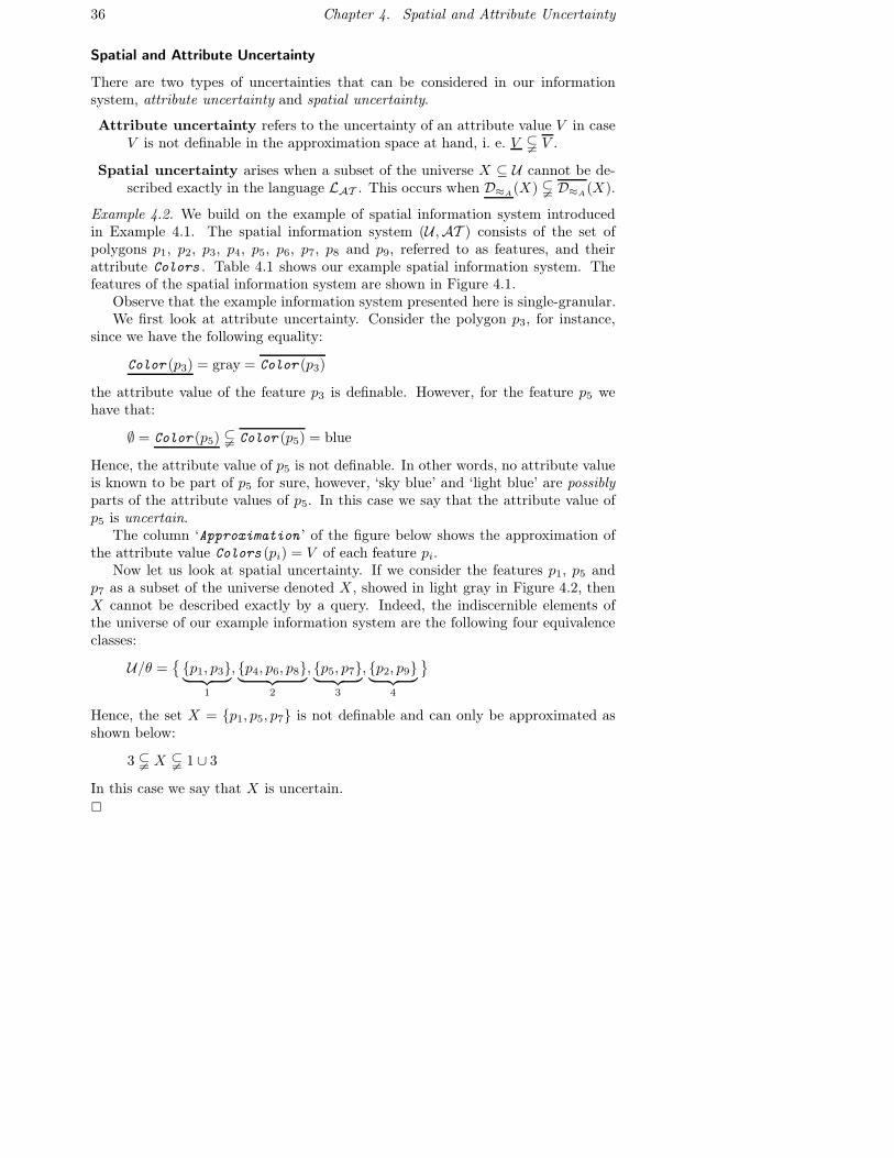
36 Chapter 4. Spatial and Attribute Uncertainty
Spatial and Attribute Uncertainty
There are two types of uncertainties that can be considered in our informationsystem, attribute uncertainty and spatial uncertainty.
Attribute uncertainty refers to the uncertainty of an attribute value V in caseV is not definable in the approximation space at hand, i. e. V � V .
Spatial uncertainty arises when a subset of the universe X ⊆ U cannot be de-scribed exactly in the language LAT . This occurs when D≈A(X) � D≈A(X).
Example 4.2. We build on the example of spatial information system introducedin Example 4.1. The spatial information system (U ,AT ) consists of the set ofpolygons p1, p2, p3, p4, p5, p6, p7, p8 and p9, referred to as features, and theirattribute Colors . Table 4.1 shows our example spatial information system. Thefeatures of the spatial information system are shown in Figure 4.1.
Observe that the example information system presented here is single-granular.We first look at attribute uncertainty. Consider the polygon p3, for instance,
since we have the following equality:
Color (p3) = gray = Color (p3)
the attribute value of the feature p3 is definable. However, for the feature p5 wehave that:
∅ = Color (p5) � Color (p5) = blue
Hence, the attribute value of p5 is not definable. In other words, no attribute valueis known to be part of p5 for sure, however, ‘sky blue’ and ‘light blue’ are possiblyparts of the attribute values of p5. In this case we say that the attribute value ofp5 is uncertain.
The column ‘Approximation ’ of the figure below shows the approximation ofthe attribute value Colors (pi) = V of each feature pi.
Now let us look at spatial uncertainty. If we consider the features p1, p5 andp7 as a subset of the universe denoted X , showed in light gray in Figure 4.2, thenX cannot be described exactly by a query. Indeed, the indiscernible elements ofthe universe of our example information system are the following four equivalenceclasses:
U/θ ={{p1, p3}︸ ︷︷ ︸
1
, {p4, p6, p8}︸ ︷︷ ︸2
, {p5, p7}︸ ︷︷ ︸3
, {p2, p9}︸ ︷︷ ︸4
}
Hence, the set X = {p1, p5, p7} is not definable and can only be approximated asshown below:
3 � X � 1 ∪ 3
In this case we say that X is uncertain.�
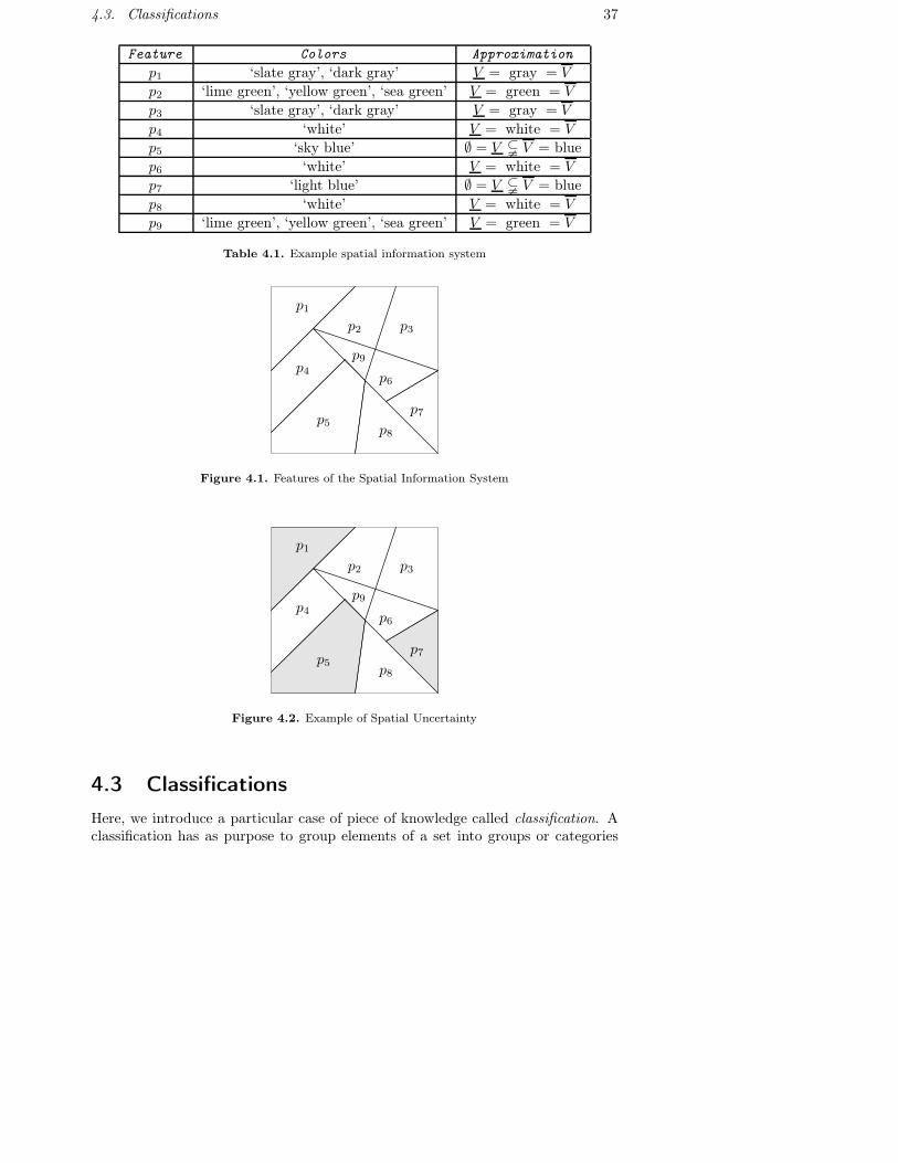
4.3. Classifications 37
Feature Colors Approximationp1 ‘slate gray’, ‘dark gray’ V = gray = V
p2 ‘lime green’, ‘yellow green’, ‘sea green’ V = green = V
p3 ‘slate gray’, ‘dark gray’ V = gray = V
p4 ‘white’ V = white = V
p5 ‘sky blue’ ∅ = V � V = bluep6 ‘white’ V = white = V
p7 ‘light blue’ ∅ = V � V = bluep8 ‘white’ V = white = V
p9 ‘lime green’, ‘yellow green’, ‘sea green’ V = green = V
Table 4.1. Example spatial information system
p1
p2 p3
p4
p5
p6
p7
p8
p9
Figure 4.1. Features of the Spatial Information System
p1
p2 p3
p4
p5
p6
p7
p8
p9
Figure 4.2. Example of Spatial Uncertainty
4.3 ClassificationsHere, we introduce a particular case of piece of knowledge called classification. Aclassification has as purpose to group elements of a set into groups or categories
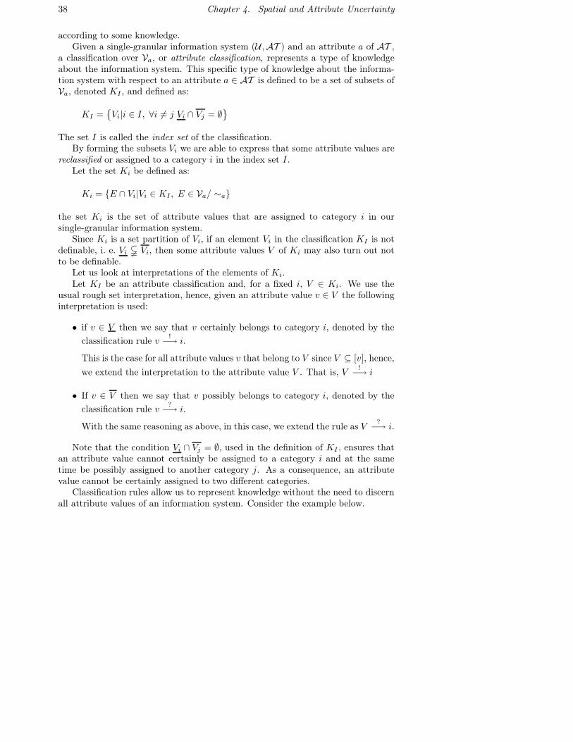
38 Chapter 4. Spatial and Attribute Uncertainty
according to some knowledge.Given a single-granular information system (U ,AT ) and an attribute a of AT ,
a classification over Va, or attribute classification, represents a type of knowledgeabout the information system. This specific type of knowledge about the informa-tion system with respect to an attribute a ∈ AT is defined to be a set of subsets ofVa, denoted KI , and defined as:
KI ={Vi|i ∈ I, ∀i = j Vi ∩ Vj = ∅
}
The set I is called the index set of the classification.By forming the subsets Vi we are able to express that some attribute values are
reclassified or assigned to a category i in the index set I.Let the set Ki be defined as:
Ki = {E ∩ Vi|Vi ∈ KI , E ∈ Va/ ∼a}
the set Ki is the set of attribute values that are assigned to category i in oursingle-granular information system.
Since Ki is a set partition of Vi, if an element Vi in the classification KI is notdefinable, i. e. Vi � Vi, then some attribute values V of Ki may also turn out notto be definable.
Let us look at interpretations of the elements of Ki.Let KI be an attribute classification and, for a fixed i, V ∈ Ki. We use the
usual rough set interpretation, hence, given an attribute value v ∈ V the followinginterpretation is used:
• if v ∈ V then we say that v certainly belongs to category i, denoted by theclassification rule v
!−→ i.
This is the case for all attribute values v that belong to V since V ⊆ [v], hence,we extend the interpretation to the attribute value V . That is, V
!−→ i
• If v ∈ V then we say that v possibly belongs to category i, denoted by theclassification rule v
?−→ i.
With the same reasoning as above, in this case, we extend the rule as V?−→ i.
Note that the condition Vi ∩ Vj = ∅, used in the definition of KI , ensures thatan attribute value cannot certainly be assigned to a category i and at the sametime be possibly assigned to another category j. As a consequence, an attributevalue cannot be certainly assigned to two different categories.
Classification rules allow us to represent knowledge without the need to discernall attribute values of an information system. Consider the example below.

4.3. Classifications 39
Example 4.3. As an example, assume we wish to state that the colors ‘lime green’,‘yellow green’ and ‘medium sea green’ indicate the presence of vegetation, we buildthe attribute classification with the following rules:
lg !−→ vegetation, yg !−→ vegetation, mg !−→ vegetation,
The knowledge above needs an ability to discern these colors, however, using thegeneralized rule defined above, using the same settings as of Example 4.1, one canstate:
green !−→ vegetation
The ‘green’ color, in accordance with the equivalence relation that we have chosen,is also relatively easy to discern.
Now suppose we have some additional knowledge about identification of veget-ation wetness, wet vegetation and dry vegetation for instance. Assume that theknowledge is set as follows: ‘medium sea green’ indicates wet vegetation and ‘limegreen’ may indicate wet vegetation as well as dry vegetation and ‘yellow green’indicates dry vegetation. The attribute classification is built as:
Kwetness ={Vwet = {medium sea green, lime green},
Vdry = {lime green, yellow green}}
Vwet and Vdry are not definable since ∅ = Vwet = Vdry � Vwet = Vdry = green. Theattribute classification induces the following rules:
medium sea green ?−→ wet, lime green ?−→ wet,
lime green ?−→ dry, yellow green ?−→ dry,
Again, since the knowledge above needs an ability to discern ‘medium sea green’,‘lime green’ and ‘yellow green’ from each other, we may use the generalized rules:
green ?−→ wet and green ?−→ dry
Hence, the information system together with our knowledge do not provide enoughinformation to discern between wet and dry vegetation by means of the green color.As a consequence, parcels of lands with wet vegetation and parcels of land with dryvegetation become uncertain since they cannot be discerned from each other.�
Below we show how to use attribute classifications in queries to the informationsystem.
40 Chapter 4. Spatial and Attribute Uncertainty
4.4 Querying ClassificationsGiven an information system (U ,AT ) and a classification KI over Va, we wishto query the information system about elements of the universe according to thecategories of I. In other terms, we would like to retrieve elements of the universethat have been classified to a certain category i ∈ I. For this purpose we define twoquery operators, the lower and the upper query operators defined respectively as:
�a = Vi� ={|a = E|
∣∣ E ⊆ Vi, E ∈ Va/ ∼a
}
�a = Vi� ={|a = E ∩ Vi|
∣∣ E ∩ Vi = ∅, E ∈ Va/ ∼a
}
Note that �a = Vi� ⊆ �a = Vi� and that (�a = Vi�, �a = Vi�) is a rough set in theapproximation space (U , θa). We say that it is a rough set built out of queries.
We define a universal classification as a classification over the universe U thatis induced by an attribute classification KI . The universal classification inducedby KI is denoted [KI ] and is defined to be a set of rough sets (�a = Vi�, �a = Vi�),where Vi ∈ KI .
A rough set (�a = Vi�, �a = Vi�) is characterized follows:
• the lower classification query �a = Vi� is said to be the lower approximationof the rough set and returns elements of the universe whose attribute valuessurely belong to i.
• the upper classification query �a = Vi� is said to be the upper approximationof the rough set and returns elements of the universe whose attribute valuespossibly belong to i.
It is important to note that, in general, as for usual rough sets, the followinginequalities hold for rough sets built out of queries:
�a = Vi ∪ Vj� = �a = Vi� ∪ �a = Vj��a = Vi ∩ Vj� = �a = Vi� ∩ �a = Vj�
Moreover, upper and lower classification queries approximate an unknown set X ⊆U , hence, we do not have a representative for the rough set R = (�a = Vi�, �a = Vi�).It turns out, however, that in the case of upper and lower classification query oper-ations used with single-granular attribute values, i. e. Vi/ ∼a is a singleton for alli, the attribute value Vi may be considered as a set representative for R. As a con-sequence, union and intersection of lower and upper queries may be truth-functionalif we restrict the domain to (Va)AB using the truth-functional set representativesof Section 3.2.3, for instance. If all the elements Vi of an attribute classification KI
belong to (Va)AB, then, the following hold:
�a = Vi ∪ Vj� = �a = Vi� ∪ �a = Vj� (4.3)
�a = Vi ∩ Vj� = �a = Vi� ∩ �a = Vj� (4.4)The attribute classification is said to be truth-functional.
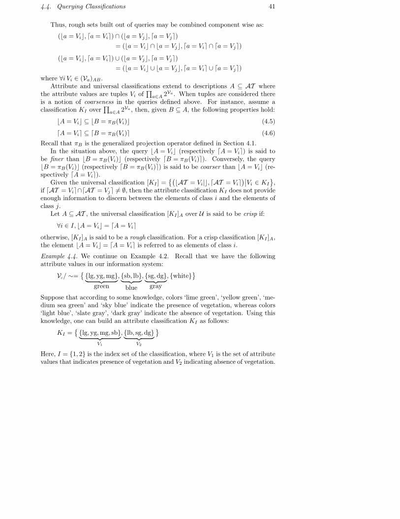
4.4. Querying Classifications 41
Thus, rough sets built out of queries may be combined component wise as:
(�a = Vi�, �a = Vi�) ∩ (�a = Vj�, �a = Vj�)= (�a = Vi� ∩ �a = Vj�, �a = Vi� ∩ �a = Vj�)
(�a = Vi�, �a = Vi�) ∪ (�a = Vj�, �a = Vj�)= (�a = Vi� ∪ �a = Vj�, �a = Vi� ∪ �a = Vj�)
where ∀i Vi ∈ (Va)AB .Attribute and universal classifications extend to descriptions A ⊆ AT where
the attribute values are tuples Vi of∏
a∈A 2Va . When tuples are considered thereis a notion of coarseness in the queries defined above. For instance, assume aclassification KI over
∏a∈A 2Va , then, given B ⊆ A, the following properties hold:
�A = Vi� ⊆ �B = πB(Vi)� (4.5)
�A = Vi� ⊆ �B = πB(Vi)� (4.6)Recall that πB is the generalized projection operator defined in Section 4.1.
In the situation above, the query �A = Vi� (respectively �A = Vi�) is said tobe finer than �B = πB(Vi)� (respectively �B = πB(Vi)�). Conversely, the query�B = πB(Vi)� (respectively �B = πB(Vi)�) is said to be coarser than �A = Vi� (re-spectively �A = Vi�).
Given the universal classification [KI ] ={(
�AT = Vi|�, �AT = Vi�)∣∣Vi ∈ KI
},
if �AT = Vi�∩�AT = Vj� = ∅, then the attribute classification KI does not provideenough information to discern between the elements of class i and the elements ofclass j.
Let A ⊆ AT , the universal classification [KI ]A over U is said to be crisp if:
∀i ∈ I, �A = Vi� = �A = Vi�otherwise, [KI ]A is said to be a rough classification. For a crisp classification [KI ]A,the element �A = Vi� = �A = Vi� is referred to as elements of class i.
Example 4.4. We continue on Example 4.2. Recall that we have the followingattribute values in our information system:
Vc/ ∼={{lg, yg, mg}︸ ︷︷ ︸
green, {sb, lb}︸ ︷︷ ︸
blue
, {sg, dg}︸ ︷︷ ︸gray
, {white}}
Suppose that according to some knowledge, colors ‘lime green’, ‘yellow green’, ‘me-dium sea green’ and ‘sky blue’ indicate the presence of vegetation, whereas colors‘light blue’, ‘slate gray’, ‘dark gray’ indicate the absence of vegetation. Using thisknowledge, one can build an attribute classification KI as follows:
KI ={{lg, yg, mg, sb}︸ ︷︷ ︸
V1
, {lb, sg, dg}︸ ︷︷ ︸V2
}
Here, I = {1, 2} is the index set of the classification, where V1 is the set of attributevalues that indicates presence of vegetation and V2 indicating absence of vegetation.
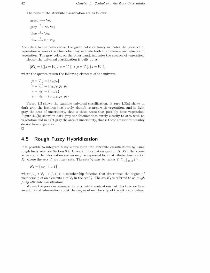
42 Chapter 4. Spatial and Attribute Uncertainty
The rules of the attribute classification are as follows:
green !−→ Veg
gray !−→ No Veg
blue ?−→ Veg
blue ?−→ No Veg
According to the rules above, the green color certainly indicates the presence ofvegetation whereas the blue color may indicate both the presence and absence ofvegetation. The gray color, on the other hand, indicates the absence of vegetation.
Hence, the universal classification is built up as:
[KI ] = {(�a = V1�, �a = V1�), (�a = V2�, �a = V2�)}
where the queries return the following elements of the universe:
�a = V1� = {p2, p9}�a = V1� = {p2, p9, p5, p7}�a = V2� = {p1, p3}�a = V2� = {p1, p3, p5, p7}
Figure 4.3 shows the example universal classification. Figure 4.3(a) shows indark gray the features that surely classify to area with vegetation, and in lightgray the area of uncertainty, that is those areas that possibly have vegetation.Figure 4.3(b) shows in dark gray the features that surely classify to area with novegetation and in light gray the area of uncertainty, that is those areas that possiblydo not have vegetation.�
4.5 Rough Fuzzy HybridizationIt is possible to integrate fuzzy information into attribute classifications by usingrough fuzzy sets, see Section 3.4. Given an information system (U ,AT ) the know-ledge about the information system may be expressed by an attribute classificationKI where the sets Vi are fuzzy sets. The sets Vi may be tuples Vi ⊆
∏a∈A 2Va .
KI = {µVi | i ∈ I}
where µVi : Va → [0, 1] is a membership function that determines the degree ofmembership of an elements v of Va in the set Vi. The set KI is referred to as roughfuzzy attribute classification.
We use the previous semantic for attribute classifications but this time we havean additional information about the degree of membership of the attribute values.
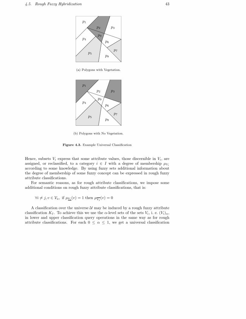
4.5. Rough Fuzzy Hybridization 43
p1
p2 p3
p4
p5
p6
p7
p8
p9
(a) Polygons with Vegetation.
p1
p2 p3
p4
p5
p6
p7
p8
p9
(b) Polygons with No Vegetation.
Figure 4.3. Example Universal Classification
Hence, subsets Vi express that some attribute values, those discernible in Vi, areassigned, or reclassified, to a category i ∈ I with a degree of membership µVi
according to some knowledge. By using fuzzy sets additional information aboutthe degree of membership of some fuzzy concept can be expressed in rough fuzzyattribute classifications.
For semantic reasons, as for rough attribute classifications, we impose someadditional conditions on rough fuzzy attribute classifications, that is:
∀i = j, v ∈ Va, if µVi(v) = 1 then µVj(v) = 0
A classification over the universe U may be induced by a rough fuzzy attributeclassification KI . To achieve this we use the α-level sets of the sets Vi, i. e. (Vi)α,in lower and upper classification query operations in the same way as for roughattribute classifications. For each 0 ≤ α ≤ 1, we get a universal classification
44 Chapter 4. Spatial and Attribute Uncertainty
[(KI)α] over U defined as:
[(KI)α
]=
{(�a = (Vi)α�, �a = (Vi)α�
) ∣∣ α ∈ [0, 1], i ∈ I}
4.6 ConclusionWe have defined a query language based on the one by Marek et al. [MT99]. Ourquery language is more powerful in the sense that it allows the representation ofattribute uncertainty. Moreover, in our model, there is a clear relation betweenattribute and spatial uncertainty.
Based on queries of attribute classifications, we have defined rough and roughfuzzy universal classifications. We have shown that they are suitable to representuncertainty in classifications.
We have shown that intersection and union of queries can be made truth-functional and that, as a consequence, rough sets built out of queries can be com-bined through intersection and union operators. Truth-functionality turns out tobe an important property as it is necessary to intersect elements of a universalclassification to measure the areas of uncertainty. When intersection is performedover all the elements of a universal classification we say that we perform an overlayoperation. Chapter 7 presents some experiments on the use of the overlay operation.
Chapter 5
Accuracy Assessments
In this chapter we present ways to assess the accuracy of classifications. Section 5.1recalls some methods used to assess accuracy of crisp classifications. Sections 5.2and 5.3 present some methods to assess accuracy of rough, respectively rough fuzzy,classifications. Finally, in Section 5.4, we present a way to assess topological rela-tions between rough classifications.
5.1 Accuracy Assessment of Crisp Classifications
Let (U ,AT ) be an information system, and let XI and YI be two attribute classi-fications over
∏a∈A 2Va , i. e. Xi, Yi ⊆
∏a∈A 2Va , inducing two crisp classifications
[XI ] and [YI ] over U . Recall that for a crisp classification lower and upper approx-imations are equal, i. e. �Xi� = �Xi�, denoted Xi. Suppose we wish to compareclassification [YI ] against [XI ], i. e. see how well Xi and Yi match for all i ∈ I.The reference classification is chosen to be [XI ] and [YI ] is the classification thatis being assessed. To achieve the comparison we will be using an error matrix asdescribed in [Con91].
First, we define the cardinality, or total area, of a crisp classification [XI ] as:
∣∣[XI ]∣∣ =
∣∣ ⋃i∈I
Xi
∣∣ =∑i∈I
∣∣Xi
∣∣.
The error matrix is defined to be a |I|×|I| matrix where the columns correspondto the reference classification [XI ] and the rows to the classification that is to beassessed, i. e. [YI ]. The cells of the matrix are elements zi,j such that zi,j = |Xi∩Yj |.The error matrix has the following three properties:
• The row-sum property:∑
j zi,j = |Yi|, i. e. the sum of the elements in a singlerow of the matrix is the area of the corresponding element of [YI ].
45
46 Chapter 5. Accuracy Assessments
• The column-sum property:∑
i zi,j = |Xj |, i. e. the sum of the elements in asingle column of the matrix is the area of the corresponding element of [XI ].
• The total-sum property:∑
i,j zi,j =∣∣[XI ]
∣∣ =∣∣[YI ]
∣∣, i. e. the sum of all theelements of the matrix is the area covered by either of the classifications [XI ]or [YI ].
Let A =∣∣[XI ]
∣∣ =∣∣[YI ]
∣∣ be the total area of the classifications. The overallaccuracy is defined as the total match between the two classifications divided bythe total area of the classifications:
Ao =∑
i
zi,i/A (5.1)
In a similar manner, one can compute the accuracy of individual classes withthe choice of dividing the correctly classified area, i. e. zi,i for class i, by either |Xi|or |Yi|. Assuming that the reference classification is associated with the columnsof the matrix, dividing by the column total gives the omission error, also calledproducer’s accuracy; dividing by the row total gives the commission error, alsocalled user’s accuracy. They are defined respectively as follows:
Oj = zj,j/∑
i
zi,j , and Ci = zi,i/∑
j
zi,j (5.2)
5.2 Accuracy Assessment of Rough ClassificationsWe present some measures that can be used to assess accuracy of rough classifica-tions.
5.2.1 The Overlap and the Crispness MeasuresThe overlap measure, denoted O, is a measure that applies to a single rough clas-sification [XI ] measuring the degree of overlap. O is defined as:
O =( ∑
i∈I
|�Xi�| − A)/
A
where A is the total area of the classification [XI ]; |I| is the number of classes orattributes of the classification. The degree of overlap increases with the amount ofoverlapping upper approximations �Xi� indicating the degree of uncertainty. Themore there is overlap, the more uncertain the classification is.
The interval 0 ≤ O ≤ |I| − 1 is interpreted as follows: if the overlap measure isequal to |I| − 1 the rough classification is completely rough, i. e. the lower approx-imations �Xi� are all empty. An overlap measure equal to 0, on the other hand,indicates that the rough classification is completely crisp, i. e. areas of uncertainty(�Xi� \ �Xi�) are all empty.

5.2. Accuracy Assessment of Rough Classifications 47
A similar measure is the crispness measure C defined as:
C =( ∑
i∈I
|�Xi�|)/
A
It takes values between 0, which indicates that the classification is completely un-certain, and 1, which indicates that the classification is completely crisp.
5.2.2 Comparing Rough Classifications
As previously, we have two rough classifications over U , [XI ] and [YI ], and wewish to compare [YI ] against the reference classification [XI ]. In a rough classi-fication [XI ], we might have that �Xi� = �Xi� for some attribute i ∈ I, hence,we cannot directly apply the accuracy measures seen in Section 5.1. The reasonis that
∣∣[XI ]∣∣ =
∣∣ ⋃i∈I�Xi�
∣∣ = ∑i∈I
∣∣�Xi�∣∣. Indeed, in a rough classification [XI ],
the upper approximation of two different classes �Xi� and �Xj� may overlap, i. e.�Xi� ∩ �Xj� = ∅. Hence, some element might be counted more than once whencalculating
∣∣[XI ]∣∣. To overcome this we transform rough classifications into virtual
crisp ones, also called parameterized crisp classifications.
5.2.3 Parameterized Crisp Classifications
To transform a rough classification into a parameterized crisp classification we in-troduce a parameter on subsets that are shared between some attributes C ⊆ I, wecall them rough components. A rough component is a subset of U that is in all theareas of uncertainty of the classes that are members of C, and in none of the areasof uncertainty of any of the classes that are not members of C. Hence, a roughcomponent is defined as:
RC =⋂i∈C
(�Xi� \ �Xi�
)\
⋃i�∈C
(�Xi� \ �Xi�
).
To each class, or attribute i ∈ I, in a rough classification [XI ], corresponds aset of rough components Γi, whose elements are referred to as rough componentsof class i, defined as:
Γi = {RC |i ∈ C, C ⊆ I}
Hence, by considering the possible assignments of the elements of Γi to the sharedclasses we can arrive at a crisp classification that is parameterized over the assign-ment possibilities. The parameterization is achieved by using a set of |I| parameterfunctions fi, i ∈ I, associated with the classification [XI ]. Each parameter functionfi corresponds to a class, or attribute i ∈ I. We require the parameter functions fi
to satisfy the following properties:
48 Chapter 5. Accuracy Assessments
∀A ⊆ U ,⋃i∈I
fi(A) = A
∀i, ∀A, B ⊆ U , fi(A ∪ B) = fi(A) ∪ fi(B)
∀i, ∀A, B ⊆ U , fi(A ∩ B) = fi(A) ∩ fi(B)
∀i, j, i = j, ∀A, B ⊆ U , fi(A) ∩ fj(B) = ∅Now we are able to express the rough classification [XI ] in terms of a paramet-
erized crisp classification XI as:
XI ={�Xi� ∪ fi(Γi)|i ∈ I
}.
We are now able to compute the cardinality∣∣[XI ]
∣∣ since there is no overlapbetween upper approximations, i. e. ∀i, j, i = j, fi(Γi) ∩ fj(Γj) = ∅. Functions fi
translate to scalar parameters as follows:
∀A ⊆ U , |A| = |⋃i∈I
fi(A)| =∑i∈I
|fi(A)|,
hence, |fi(A)| = xi · |A| where 0 ≤ xi ≤ 1 and∑
i∈I xi = 1.Applied to the cardinality of the parameterized crisp classification XI , |XI | is
the sum of the cardinalities of all classes Xi, thus, |XI | =∑
i∈I |Xi|. The cardinalityof a class Xi depends on the parameter function fi:
∀i ∈ I, |Xi| =∣∣�Xi� ∪ fi(Γi))
∣∣ =∣∣�Xi�
∣∣ + |fi(Γi)| =∣∣�Xi�
∣∣ +∑
K∈Γi
xi,K · |K|,
we also have to put some restrictions on the parameters xi,K :
∀K ∈ Γi, 0 ≤ xi,K ≤ 1 and∑
i
xi,K = 1
5.2.4 Parameterized Error MatrixIt is possible to build an error matrix to compare a rough classification [XI ] witha crisp classification YI or to compare two rough classifications [XI ] and [YI ] witheach other. In both cases we build a |I|× |I| matrix with elements xi,j . In the casewhere [XI ] is rough and [YI ] is crisp the element xi,j writes as:

5.2. Accuracy Assessment of Rough Classifications 49
xi,j = |Xi ∩ Yj | =∣∣(�Xi� ∪ fi(Γi)
)∩ Yj
∣∣ =∣∣�Xi� ∩ Yj
∣∣ + |fi(Γi) ∩ Yj |
=∣∣�Xi� ∩ Yj
∣∣ +∣∣ ⋃
K∈Γi
(fi(K)
)∩ Yj
∣∣ =∣∣�Xi� ∩ Yj
∣∣ +∣∣ ⋃
K∈Γi
(fi(K) ∩ Yj
)∣∣=
∣∣�Xi� ∩ Yj
∣∣ +∣∣ ⋃
K∈Γi
(fi(K ∩ Yj)
)∣∣ =∣∣�Xi� ∩ Yj
∣∣ +∑
K∈Γi
xi,K · |K ∩ Yj |
(5.3)
where fi ∈ FXI and the following conditions on the parameters hold:
0 ≤ xi,K ≤ 1 and∑
i
xi,K = 1.
If both [XI ] and [YI ] are rough, [YI ] should also be transformed to a parameterizedcrisp classification. We therefore introduce R′
C defined as:
R′C =
⋂i∈C
(�Yi� \ �Yi�
)\
⋃i�∈C
(�Yi� \ �Yi�
),
and the set of rough components of [YI ] defined as ∆i = {R′C |i ∈ C, C ⊆ I}. We
then use the parameterized crisp classification YI ={�Yi� ∪ gi(∆i)|i ∈ I
}, where
gi, i ∈ I, are parameter functions associated with classification [YI ] with the sameproperties as the parameter function fi above. In this situation, xi,j writes as:
xi,j = |Xi ∩ Yj | =∣∣(�Xi� ∪ fi(Γi)
)∩
(�Yj� ∪ gj(∆j)
)∣∣=
∣∣�Xi� ∩ �Yj�∣∣ +
∑K∈Γi
xi,K ·∣∣K ∩ �Yj�
∣∣ +∑
L∈∆j
xj,L ·∣∣�Xi� ∩ L
∣∣+
∑K∈Γi
∑L∈∆j
|fi(K) ∩ gj(L)|
=∣∣�Xi� ∩ �Yj�
∣∣ +∑
K∈Γi
xi,K ·∣∣K ∩ �Yj�
∣∣ +∑
L∈∆j
xj,L ·∣∣�Xi� ∩ L
∣∣+
∑K∈Γi
∑L∈∆j
|fi(K ∩ gj(L))|
=∣∣�Xi� ∩ �Yj�
∣∣ +∑
K∈Γi
xi,K ·∣∣K ∩ �Yj�
∣∣ +∑
L∈∆j
xj,L · +∣∣�Xi� ∩ L
∣∣+
∑K∈Γi
∑L∈∆j
xi,K · |K ∩ gj(L))|
=∣∣�Xi� ∩ �Yj�
∣∣ +∑
K∈Γi
xi,K ·∣∣K ∩ �Yj�
∣∣ +∑
L∈∆j
xj,L ·∣∣�Xi� ∩ L +
∣∣+
∑K∈Γi
∑L∈∆j
xi,K · xj,L · |K ∩ L|
(5.4)
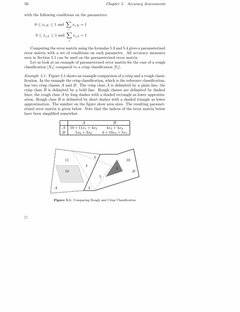
50 Chapter 5. Accuracy Assessments
with the following conditions on the parameters:
0 ≤ xi,K ≤ 1 and∑
i
xi,K = 1
0 ≤ xj,L ≤ 1 and∑
j
xj,L = 1
Computing the error matrix using the formulas 5.3 and 5.4 gives a parameterizederror matrix with a set of conditions on each parameter. All accuracy measuresseen in Section 5.1 can be used on the parameterized error matrix.
Let us look at an example of parameterized error matrix for the case of a roughclassification [XI ] compared to a crisp classification [YI ].
Example 5.1. Figure 5.1 shows an example comparison of a crisp and a rough classi-fication. In the example the crisp classification, which is the reference classification,has two crisp classes A and B. The crisp class A is delimited by a plain line, thecrisp class B is delimited by a bold line. Rough classes are delimited by dashedlines, the rough class A by long dashes with a shaded rectangle as lower approxim-ation. Rough class B is delimited by short dashes with a shaded triangle as lowerapproximation. The number on the figure show area sizes. The resulting paramet-erized error matrix is given below. Note that the indices of the error matrix belowhave been simplified somewhat:
A BA 10 + 11x1 + 4x2 4x3 + 4x4
B 5x6 + 3x8 4 + 10x5 + 5x7
11
10
3
4
4
5
4
10
A
B
Figure 5.1. Comparing Rough and Crisp Classification
�
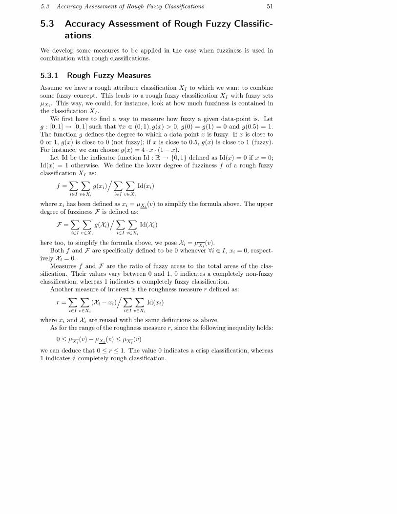
5.3. Accuracy Assessment of Rough Fuzzy Classifications 51
5.3 Accuracy Assessment of Rough Fuzzy Classific-ations
We develop some measures to be applied in the case when fuzziness is used incombination with rough classifications.
5.3.1 Rough Fuzzy MeasuresAssume we have a rough attribute classification XI to which we want to combinesome fuzzy concept. This leads to a rough fuzzy classification XI with fuzzy setsµXi . This way, we could, for instance, look at how much fuzziness is contained inthe classification XI .
We first have to find a way to measure how fuzzy a given data-point is. Letg : [0, 1] → [0, 1] such that ∀x ∈ (0, 1), g(x) > 0, g(0) = g(1) = 0 and g(0.5) = 1.The function g defines the degree to which a data-point x is fuzzy. If x is close to0 or 1, g(x) is close to 0 (not fuzzy); if x is close to 0.5, g(x) is close to 1 (fuzzy).For instance, we can choose g(x) = 4 · x · (1 − x).
Let Id be the indicator function Id : R → {0, 1} defined as Id(x) = 0 if x = 0;Id(x) = 1 otherwise. We define the lower degree of fuzziness f of a rough fuzzyclassification XI as:
f =∑i∈I
∑v∈Xi
g(xi)/ ∑
i∈I
∑v∈Xi
Id(xi)
where xi has been defined as xi = µXi(v) to simplify the formula above. The upperdegree of fuzziness F is defined as:
F =∑i∈I
∑v∈Xi
g(Xi)/ ∑
i∈I
∑v∈Xi
Id(Xi)
here too, to simplify the formula above, we pose Xi = µXi(v).
Both f and F are specifically defined to be 0 whenever ∀i ∈ I, xi = 0, respect-ively Xi = 0.
Measures f and F are the ratio of fuzzy areas to the total areas of the clas-sification. Their values vary between 0 and 1, 0 indicates a completely non-fuzzyclassification, whereas 1 indicates a completely fuzzy classification.
Another measure of interest is the roughness measure r defined as:
r =∑i∈I
∑v∈Xi
(Xi − xi)/ ∑
i∈I
∑v∈Xi
Id(xi)
where xi and Xi are reused with the same definitions as above.As for the range of the roughness measure r, since the following inequality holds:
0 ≤ µXi(v) − µXi(v) ≤ µXi
(v)
we can deduce that 0 ≤ r ≤ 1. The value 0 indicates a crisp classification, whereas1 indicates a completely rough classification.
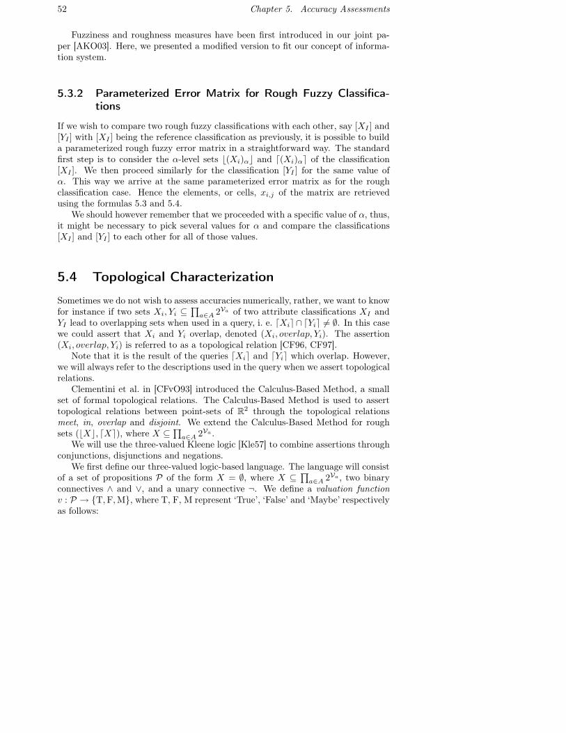
52 Chapter 5. Accuracy Assessments
Fuzziness and roughness measures have been first introduced in our joint pa-per [AKO03]. Here, we presented a modified version to fit our concept of informa-tion system.
5.3.2 Parameterized Error Matrix for Rough Fuzzy Classifica-tions
If we wish to compare two rough fuzzy classifications with each other, say [XI ] and[YI ] with [XI ] being the reference classification as previously, it is possible to builda parameterized rough fuzzy error matrix in a straightforward way. The standardfirst step is to consider the α-level sets �(Xi)α� and �(Xi)α� of the classification[XI ]. We then proceed similarly for the classification [YI ] for the same value ofα. This way we arrive at the same parameterized error matrix as for the roughclassification case. Hence the elements, or cells, xi,j of the matrix are retrievedusing the formulas 5.3 and 5.4.
We should however remember that we proceeded with a specific value of α, thus,it might be necessary to pick several values for α and compare the classifications[XI ] and [YI ] to each other for all of those values.
5.4 Topological Characterization
Sometimes we do not wish to assess accuracies numerically, rather, we want to knowfor instance if two sets Xi, Yi ⊆
∏a∈A 2Va of two attribute classifications XI and
YI lead to overlapping sets when used in a query, i. e. �Xi� ∩ �Yi� = ∅. In this casewe could assert that Xi and Yi overlap, denoted (Xi, overlap, Yi). The assertion(Xi, overlap, Yi) is referred to as a topological relation [CF96, CF97].
Note that it is the result of the queries �Xi� and �Yi� which overlap. However,we will always refer to the descriptions used in the query when we assert topologicalrelations.
Clementini et al. in [CFvO93] introduced the Calculus-Based Method, a smallset of formal topological relations. The Calculus-Based Method is used to asserttopological relations between point-sets of R2 through the topological relationsmeet, in, overlap and disjoint. We extend the Calculus-Based Method for roughsets (�X�, �X�), where X ⊆
∏a∈A 2Va .
We will use the three-valued Kleene logic [Kle57] to combine assertions throughconjunctions, disjunctions and negations.
We first define our three-valued logic-based language. The language will consistof a set of propositions P of the form X = ∅, where X ⊆
∏a∈A 2Va , two binary
connectives ∧ and ∨, and a unary connective ¬. We define a valuation functionv : P → {T, F, M}, where T, F, M represent ‘True’, ‘False’ and ‘Maybe’ respectivelyas follows:

5.4. Topological Characterization 53
v(X = ∅) =
T if �X� = ∅F if �X� = ∅M otherwise
Propositions of P can be combined through the ∧, ∨ and ¬ connectives: ∀p, q ∈ P ,
v(p ∧ q) = v(p) ∧ v(q),
v(p ∨ q) = v(p) ∨ v(q),
v(¬p) = ¬v(p).
Truth values are derived using the truth tables for ∧, ∨ and ¬ below.
∧ T M FT T M FM M M FF F F F
∨ T M FT T T TM T M MF T M F
¬T FM MF T
Table 5.1. Three Valued Logic Tables for ∧, ∨ and ¬.
We extend the topological relations in, overlap and disjoint introduced in [CFvO93]to support three-valued topological relations. Our Three-valued Calculus BasedMethod (3-CBM) consists of the following topological relations:
Definition 5.2. The in 3-valued topological relation is defined as:
(X, in, Y ) ⇐⇒ (X ∩ −Y = ∅) ∧ (X ∩ Y = ∅)
Recall that −Y represents the complement of Y , so that, �−Y � = U \ �Y � and�−Y � = U \ �Y �.
Definition 5.3. The overlap 3-valued topological relation is defined as:
(X, overlap, Y ) ⇐⇒ X ∩ −Y = ∅
Definition 5.4. The disjoint 3-valued topological relation is defined as:
(X, disjoint, Y ) ⇐⇒ X ∩ Y = ∅
Thus, the topological relation (X, r, Y ), where r is one of in, overlap and disjointhas a valuation v((X, r, Y )) which is either ‘True’, ‘False’ or ‘Maybe’.
Figure 5.2 shows the topological relation decision tree of the 3-CBM, where ?rmeans v((X, r, Y )) = M and !r means v((X, r, Y )) = T . Furthermore, each branchof the tree is labeled ‘T’ (True), ‘M’ (Maybe) or ‘F’ (False) corresponding to thevaluations of the proposition of the corresponding node.
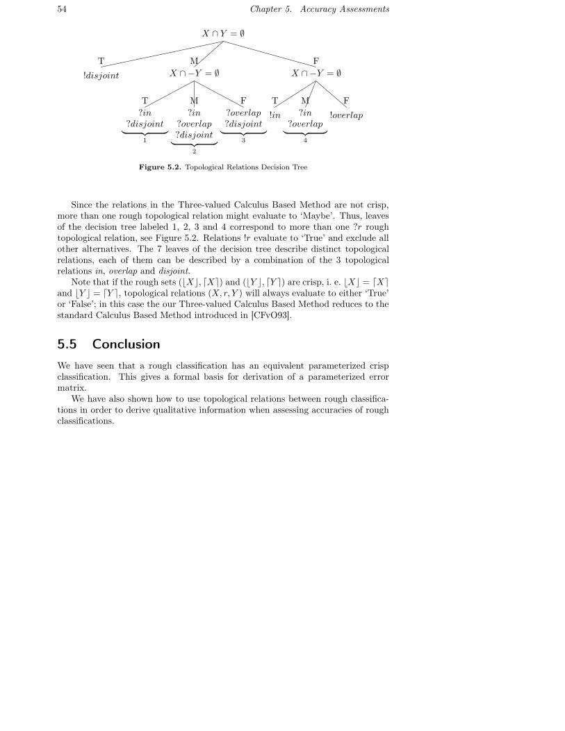
54 Chapter 5. Accuracy Assessments
!disjoint
?in?disjoint︸ ︷︷ ︸
1
?in?overlap?disjoint︸ ︷︷ ︸
2
?overlap?disjoint︸ ︷︷ ︸
3
T M F
X ∩ −Y = ∅
!in ?in?overlap︸ ︷︷ ︸
4
!overlap
T M F
X ∩ −Y = ∅T M F
X ∩ Y = ∅
Figure 5.2. Topological Relations Decision Tree
Since the relations in the Three-valued Calculus Based Method are not crisp,more than one rough topological relation might evaluate to ‘Maybe’. Thus, leavesof the decision tree labeled 1, 2, 3 and 4 correspond to more than one ?r roughtopological relation, see Figure 5.2. Relations !r evaluate to ‘True’ and exclude allother alternatives. The 7 leaves of the decision tree describe distinct topologicalrelations, each of them can be described by a combination of the 3 topologicalrelations in, overlap and disjoint.
Note that if the rough sets (�X�, �X�) and (�Y �, �Y �) are crisp, i. e. �X� = �X�and �Y � = �Y �, topological relations (X, r, Y ) will always evaluate to either ‘True’or ‘False’; in this case the our Three-valued Calculus Based Method reduces to thestandard Calculus Based Method introduced in [CFvO93].
5.5 ConclusionWe have seen that a rough classification has an equivalent parameterized crispclassification. This gives a formal basis for derivation of a parameterized errormatrix.
We have also shown how to use topological relations between rough classifica-tions in order to derive qualitative information when assessing accuracies of roughclassifications.
Chapter 6
Information System Design
This chapter shows how to implement an information system as the one presen-ted in the examples of Chapter 4 using a relational database management system(RDBMS).
Section 6.1 presents the basic relations that are required to represent indiscern-ibility. Section 6.2 shows how to approximate a relation in the database. Section 6.3shows how to use approximations in queries to the information system. Section 6.4presents a way to represent classifications using the relational model. Section 6.5discusses the truth-functional issue of approximation operators in our informationsystem.
6.1 Information Systems in the Relational ModelWe use the SQL relational language of the PostgreSQL database management sys-tem [Gro02] to implement our information system. See also [Mom01] for an intro-duction to the PostgreSQL RDBMS.
As seen in Example 4.2, the universe of our example information system is a setof features referred to by an identification number. Each feature is characterizedby a set of colors that is represented in the table ‘FeatureColors’ shown below.Note that each feature may be characterized by several colors, hence, the attribute‘colors’ below should be multi-valued. This is achieved by choosing the key of thetable below to be a combination of both attributes ‘id’ and ‘colors’:
create table FeatureColors (-- feature idid integer,-- feature colorscolors integer,primary key (id, colors)
);
55
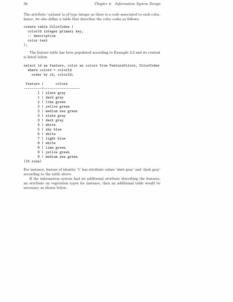
56 Chapter 6. Information System Design
The attribute ‘colors’ is of type integer as there is a code associated to each color,hence, we also define a table that describes the color codes as follows:
create table ColorCodes (colorId integer primary key,-- descriptioncolor text
);
The feature table has been populated according to Example 4.2 and its contentis listed below.
select id as feature, color as colors from FeatureColors, ColorCodeswhere colors = colorIdorder by id, colorId;
feature | colors---------+------------------
1 | slate gray1 | dark gray2 | lime green2 | yellow green2 | medium sea green3 | slate gray3 | dark gray4 | white5 | sky blue6 | white7 | light blue8 | white9 | lime green9 | yellow green9 | medium sea green
(15 rows)
For instance, feature of identity ‘1’ has attribute values ‘slate gray’ and ‘dark gray’according to the table above.
If the information system had an additional attribute describing the features,an attribute on vegetation types for instance, then an additional table would benecessary as shown below.

6.2. Approximations 57
create table FeatureVegetations (id integer,-- the attributevegetations integer,primary key (id, vegetations)
);
This way, the attribute value of the feature of identity ‘i’ may be obtained throughthe following query:
select colors, vegetationsfrom FeatureColors, FeatureVegetationswhere FeatureColors.id = i and
FeatureColors.id = FeatureVagetations.id;
Note that the statement above returns a set of tuples instead of a tuple of sets, how-ever, set results can be obtained by projecting on either attributes ‘FeatureColors’or ‘FeatureVegetations’ individually.
6.2 Approximations
Here we show how to approximate subsets of the universe given an equivalencerelation using the relational language SQL of the PostgreSQL RDBMS.
To model indiscernibility, we need an equivalence relation on the attribute valuesof ‘colors’. This equivalence relation can be defined as a Cartesian product storedin the following table:
create table EquivalentColors (colorsA integer,-- is equivalent tocolorsB integer,primary key (colorsA, colorsB)
);
Here, the primary key declaration is not necessary, however, it avoids repetition ofidentical tuples. Elements that are equivalent to each other are stored as a tuplein ‘EquivalentColors’.
The equivalence relation of our running example may be displayed as shownbelow:
select ACol.color, BCol.color fromEquivalentColors, ColorCodes as ACol, ColorCodes as BColwhere colorA = ACol.colorId and colorB = BCol.colorId;
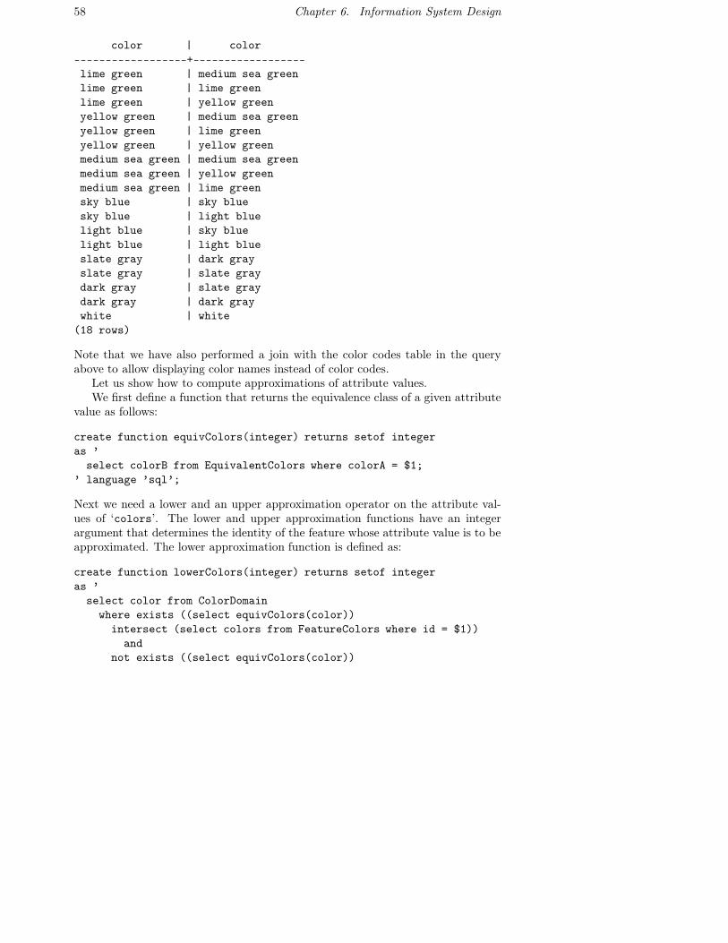
58 Chapter 6. Information System Design
color | color------------------+------------------lime green | medium sea greenlime green | lime greenlime green | yellow greenyellow green | medium sea greenyellow green | lime greenyellow green | yellow greenmedium sea green | medium sea greenmedium sea green | yellow greenmedium sea green | lime greensky blue | sky bluesky blue | light bluelight blue | sky bluelight blue | light blueslate gray | dark grayslate gray | slate graydark gray | slate graydark gray | dark graywhite | white
(18 rows)
Note that we have also performed a join with the color codes table in the queryabove to allow displaying color names instead of color codes.
Let us show how to compute approximations of attribute values.We first define a function that returns the equivalence class of a given attribute
value as follows:
create function equivColors(integer) returns setof integeras ’select colorB from EquivalentColors where colorA = $1;
’ language ’sql’;
Next we need a lower and an upper approximation operator on the attribute val-ues of ‘colors’. The lower and upper approximation functions have an integerargument that determines the identity of the feature whose attribute value is to beapproximated. The lower approximation function is defined as:
create function lowerColors(integer) returns setof integeras ’select color from ColorDomainwhere exists ((select equivColors(color))intersect (select colors from FeatureColors where id = $1))
andnot exists ((select equivColors(color))

6.2. Approximations 59
except (select colors from FeatureColors where id = $1))’ language ’sql’;
The upper approximation function is defined as:
create function upperColors(integer) returns setof integeras ’select color from ColorDomain whereexists ((select equivColors(color))intersect (select colors from FeatureColors where id = $1))
’ language ’sql’;
Above, ‘ColorDomain’ is a table that represents the domain of the attribute ‘colors.It is defined as:
create table ColorDomain (color integer primary key
);
Let us approximate the attribute value of the feature of identity ‘1’. The lowerapproximation is obtained as follows:
select lowerColor(1);
lowercolors-------------
67
The upper approximation is obtained as follows:
select upperColors(1);
uppercolors-------------
67
Since both lower and upper approximations are slate gray and dark gray, the featureof identity ‘1’ has an attribute value that is definable in our approximation space.
Let us print out the features and their approximate attribute values. The lowerapproximation of the attribute values are:
select A.id as feature, color as lower_approx from ColorCodes,(select distinct id, lowerColors(id) as i from FeatureColors) as A
where colorId = A.i order by A.id;
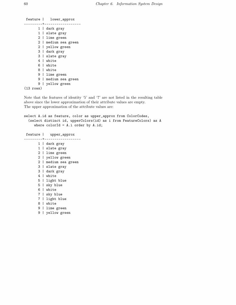
60 Chapter 6. Information System Design
feature | lower_approx---------+------------------
1 | dark gray1 | slate gray2 | lime green2 | medium sea green2 | yellow green3 | dark gray3 | slate gray4 | white6 | white8 | white9 | lime green9 | medium sea green9 | yellow green
(13 rows)
Note that the features of identity ‘5’ and ‘7’ are not listed in the resulting tableabove since the lower approximation of their attribute values are empty.The upper approximation of the attribute values are:
select A.id as feature, color as upper_approx from ColorCodes,(select distinct id, upperColors(id) as i from FeatureColors) as A
where colorId = A.i order by A.id;
feature | upper_approx---------+------------------
1 | dark gray1 | slate gray2 | lime green2 | yellow green2 | medium sea green3 | slate gray3 | dark gray4 | white5 | light blue5 | sky blue6 | white7 | sky blue7 | light blue8 | white9 | lime green9 | yellow green
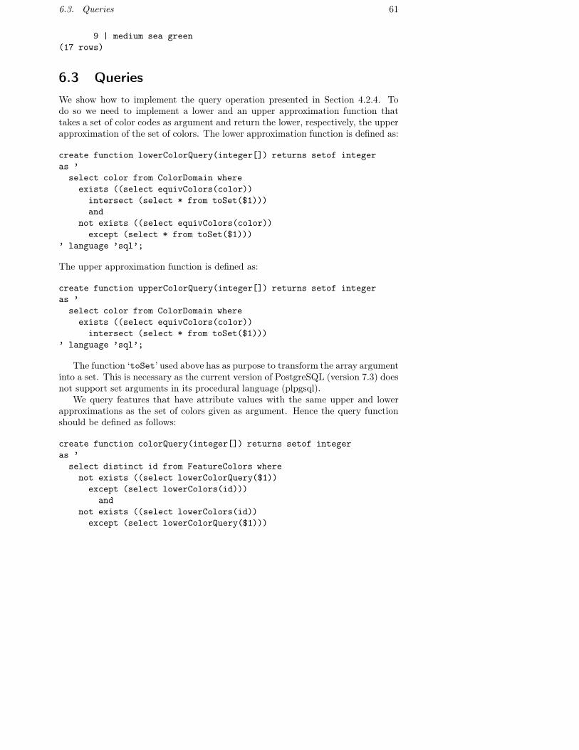
6.3. Queries 61
9 | medium sea green(17 rows)
6.3 QueriesWe show how to implement the query operation presented in Section 4.2.4. Todo so we need to implement a lower and an upper approximation function thattakes a set of color codes as argument and return the lower, respectively, the upperapproximation of the set of colors. The lower approximation function is defined as:
create function lowerColorQuery(integer[]) returns setof integeras ’select color from ColorDomain whereexists ((select equivColors(color))intersect (select * from toSet($1)))and
not exists ((select equivColors(color))except (select * from toSet($1)))
’ language ’sql’;
The upper approximation function is defined as:
create function upperColorQuery(integer[]) returns setof integeras ’select color from ColorDomain whereexists ((select equivColors(color))intersect (select * from toSet($1)))
’ language ’sql’;
The function ‘toSet’ used above has as purpose to transform the array argumentinto a set. This is necessary as the current version of PostgreSQL (version 7.3) doesnot support set arguments in its procedural language (plpgsql).
We query features that have attribute values with the same upper and lowerapproximations as the set of colors given as argument. Hence the query functionshould be defined as follows:
create function colorQuery(integer[]) returns setof integeras ’select distinct id from FeatureColors wherenot exists ((select lowerColorQuery($1))except (select lowerColors(id)))
andnot exists ((select lowerColors(id))except (select lowerColorQuery($1)))

62 Chapter 6. Information System Design
andnot exists ((select upperColorQuery($1))except (select upperColors(id)))
andnot exists ((select upperColors(id))except (select upperColorQuery($1)))
’language ’sql’;
The function defined above queries elements of the universe by means of approx-imations of attribute values. We refer to this type of query as an approximatequery.
As an example, we first query the features whose color attribute values havethe same lower and upper approximation as the singleton value ‘4’, i. e. ‘sky blue’.The second query looks for features which are approximately ‘slate gray’ and ‘darkgray’, i. e. the set of color codes ‘6’ and ‘7’.
select * from colorQuery(’{4}’);
colorquery------------
57
(2 rows)
select * from colorQuery(’{6, 7}’);
colorquery------------
13
(2 rows)
Note that the examples above are based on a single attribute ‘colors’. In casewe wish to represent queries on multiple attributes we need to implement similarrelational tables and functions as for the attribute ‘colors’. Table 6.1 outlines theattribute specific implementations for ‘colors’.
In case of an additional attribute, for instance ‘vegetations’, all tables andfunctions specified in the Table 6.1 above should be specifically implemented for the‘vegetations’ attribute. Queries would then be combinable using the intersectionand the union operators. For instance, we could query the information system asfollows:
(select colorQuery(’{1, 2}’))intersect
(select vegetationQuery(’{10}’));

6.3. Queries 63
Implementations for colors DescriptionFeatureColors stores feature’s attribute valuesColorDomain stores attribute domainColorCodes stores descriptions of color codes
EquivalentColors stores equivalence relationequivColors() in: color code, out: equivalence classlowerColors() in: feature id, out: lower colors valueupperColors() in: feature id, out: upper colors value
lowerColorQuery() in: array of color codes id, out: lower approxupperColorQuery() in: array color codes, out: upper approx
colorQuery() in: array color codes, out: features
Table 6.1. Attribute Specific Implementations for Colors
or,
(select colorQuery(’{4, 6}’))union
(select vegetationQuery(’{9, 11}’))
6.3.1 Spatial UncertaintyLet us note that the equivalence relation on the features of the information systemcan be obtained by the following query:
select distinct A.id as idA, B.id as idB into EquivalentFeaturesfrom FeatureColors as A, FeatureColors as B wherenot exists ((select lowerColors(A.id))except (select lowerColors(B.id)))and
not exists ((select lowerColors(B.id))except (select lowerColors(A.id)))and
not exists ((select upperColors(A.id))except (select upperColors(B.id)))and
not exists ((select upperColors(B.id))except (select upperColors(A.id)));
this leads to the creation of the ‘EquivalentFeatures’ table show below.
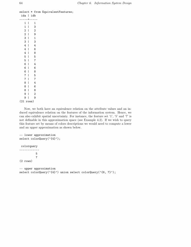
64 Chapter 6. Information System Design
select * from EquivalentFeatures;ida | idb
-----+-----1 | 11 | 32 | 22 | 93 | 13 | 34 | 44 | 64 | 85 | 55 | 76 | 46 | 66 | 87 | 57 | 78 | 48 | 68 | 89 | 29 | 9
(21 rows)
Now, we both have an equivalence relation on the attribute values and an in-duced equivalence relation on the features of the information system. Hence, wecan also exhibit spatial uncertainty. For instance, the feature set ‘1’, ‘5’ and ‘7’ isnot definable in this approximation space (see Example 4.2). If we wish to querythis feature set by means of colors descriptions we would need to compute a lowerand an upper approximation as shown below.
-- lower approximationselect colorQuery(’{4}’);
colorquery------------
57
(2 rows)
-- upper approximationselect colorQuery(’{4}’) union select colorQuery(’{6, 7}’);

6.4. Representing Classifications 65
colorquery------------
1357
(4 rows)
Thus, the feature set X = {‘1’, ‘5’, ‘7’} is not definable and has to be describedby its lower approximation: the set of features that are possibly ‘blue’ (color code‘4’ for instance) and its upper approximation: the set of features that are possibly‘blue’ or the set of features that are certainly ‘gray’:
{‘5’, ‘7’} ⊆ X ⊆ {‘1’, ‘3’, ‘5’, ‘7’}
6.4 Representing ClassificationsWe implement a table that will represent attribute classifications.
create table ColorClass (class integer primary key,colors integer[]
);
Each value of the attribute ‘colors’, as defined in Section 4.3, is an array thatrepresents the attribute values that reclassify to a category determined by the valueof the attribute ‘class’.
We continue the implementation of Example 4.4. The attribute classificationtable have been populated accordingly as follows:
select * from ColorClass
class | colors-------+-----------
1 | {1, 2, 3, 4}2 | {5, 6, 7}
(2 rows)
According to the table, features that are characterized by a ‘green’ or a ‘skyblue’ color are reclassified to category ‘1’. Features that are characterized by a‘light blue’ or a ‘gray’ color, on the other hand, are reclassified to category ‘2’. Asin the example, categories ‘1’ and ‘2’ may represent, respectively, the presence andthe absence of vegetations for instance.

66 Chapter 6. Information System Design
Again, in our approximation space the colors ‘sky blue’ and ‘light blue’ are notdiscernible, hence, we require the use of approximate queries. The universal clas-sification may be obtained by using lower and upper classification queries definedin Section 4.4. For this purpose, we implement the lower and the upper queryoperators ‘lowerClassQuery(integer[])’ and ‘upperClassQuery(integer[])’.These functions are implemented in PostgreSQL procedural language (plpgsql).The reason is that the argument of the functions has to be decomposed into a setof single-granular attribute values that form a set partition before the call to thequery function ‘colorQuery’ can be made. This decomposition requires some sideeffect operations. The code of the functions has been omitted.
The universal classification is computed below. First, the lower approximationof the attribute classification is queried:
select class, lowerClassQuery(colors) as feature from ColorClass;
class | feature-------+---------
1 | 21 | 92 | 12 | 3
(4 rows)
As it appears above, feature ‘2’ and ‘9’ surely classify to category ‘1’ and features‘1’ and ‘3’ surely classify to category ‘2’. To query features that possibly classifyto a certain category we use the upper query as shown below:
select class, upperClassQuery(colors) as feature from ColorClass;
class | feature-------+---------
1 | 21 | 51 | 71 | 92 | 12 | 32 | 52 | 7
(8 rows)
Hence, features ‘2’, ‘5’, ‘7’ and ‘9’ possibly classify to category ‘1’. Features ‘1’, ‘3’,‘5’ and ‘7’ possibly classify to category ‘2’. Also note that there is an uncertainty forthe features ‘5’ and ‘7’ since they may classify to either category ’1’ or to category

6.5. Information System and Truth Functionality 67
‘2’. Those features belong to the uncertain part of the universal classification, alsocalled the boundary of the classification.
The query �a = Vi� translates in our information system as:
select lowerClassQuery(colors)from ColorClass where class = 1;
and the query �a = Vi� translates as:
select upperClassQuery(colors) from ColorClass where class = 1;
where a corresponds to the attribute ‘colors’ and the set Vi to a set of color valuessuch as V1 = {‘1’, ‘2’, ‘3’, ‘4’} and V2 = {‘5’, ‘6’, ‘7’}.
As we noted in Section 4.4, for a given class i, the pair of queries Ci =(�a = Vi�, �a = Vi�) is a rough set. Recall that the universal classification is theset of rough sets made up of the pairs of queries Ci for each category i. To queryuncertain parts in the classification we need to perform intersections of rough sets.For instance, to query rough sets of the classification that possibly classify to bothi and j, we need to perform the intersection Ci ∩ Cj .
Below, we look at the truth-functionality issue of the intersection operator inour information system.
6.5 Information System and Truth FunctionalityTruth functionality is an issue that we have discussed in Section 3.2. Let us illustratethis in our example information system. First, we consider approximation of setsof colors. The union of lower approximations:
select lowerColorQuery(’{1,2,3,4}’) union lowerColorQuery(’{5,6,7}’);
lowercolorquery-----------------
12367
(5 rows)
is not equal to the lower approximation of the union:
select lowerColorQuery(’{1,2,3,4,5,6,7}’);
lowercolorquery-----------------
12
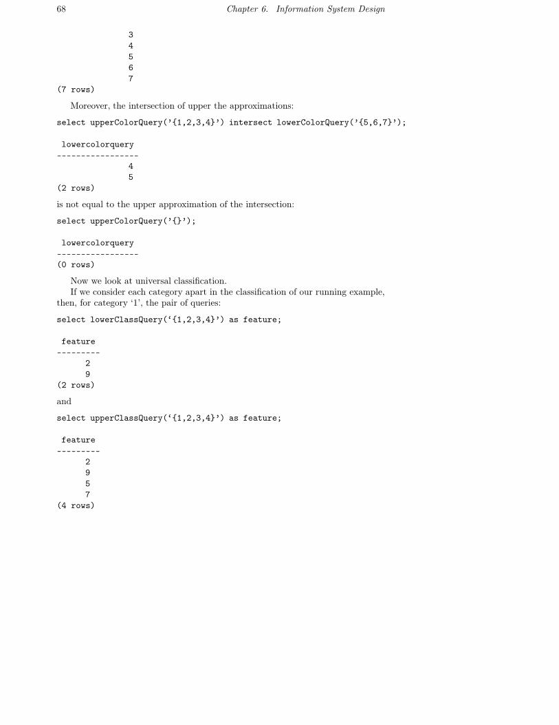
68 Chapter 6. Information System Design
34567
(7 rows)
Moreover, the intersection of upper the approximations:
select upperColorQuery(’{1,2,3,4}’) intersect lowerColorQuery(’{5,6,7}’);
lowercolorquery-----------------
45
(2 rows)
is not equal to the upper approximation of the intersection:
select upperColorQuery(’{}’);
lowercolorquery-----------------(0 rows)
Now we look at universal classification.If we consider each category apart in the classification of our running example,
then, for category ‘1’, the pair of queries:
select lowerClassQuery(‘{1,2,3,4}’) as feature;
feature---------
29
(2 rows)
and
select upperClassQuery(‘{1,2,3,4}’) as feature;
feature---------
2957
(4 rows)
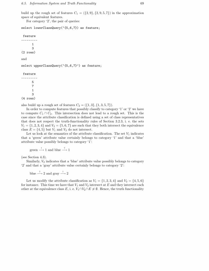
6.5. Information System and Truth Functionality 69
build up the rough set of features C1 = ({2, 9}, {2, 9, 5, 7}) in the approximationspace of equivalent features.
For category ‘2’, the pair of queries:
select lowerClassQuery(‘{5,6,7}) as feature;
feature---------
13
(2 rows)
and
select upperClassQuery(‘{5,6,7}’) as feature;
feature---------
5713
(4 rows)
also build up a rough set of features C2 = ({1, 3}, {1, 3, 5, 7}).In order to compute features that possibly classify to category ‘1’ or ‘2’ we have
to compute C1 ∩ C2. This intersection does not lead to a rough set. This is thecase since the attribute classification is defined using a set of class representativesthat does not respect the truth-functionality rules of Section 3.2.3, i. e. the setsV1 = {1, 2, 3, 4} and V2 = {5, 6, 7} are such that they both intersect the equivalenceclass E = {4, 5} but V1 and V2 do not intersect.
Let us look at the semantics of the attribute classification. The set V1 indicatesthat a ‘green’ attribute value certainly belongs to category ‘1’ and that a ‘blue’attribute value possibly belongs to category ‘1’:
green !−→ 1 and blue ?−→ 1
(see Section 4.3).Similarly, V2 indicates that a ‘blue’ attribute value possibly belongs to category
‘2’ and that a ‘gray’ attribute value certainly belongs to category ‘2’:
blue ?−→ 2 and gray !−→ 2
Let us modify the attribute classification as V1 = {1, 2, 3, 4} and V2 = {4, 5, 6}for instance. This time we have that V1 and V2 intersect at E and they intersect eachother at the equivalence class E, i. e. V1∩V2∩E = ∅. Hence, the truth functionality
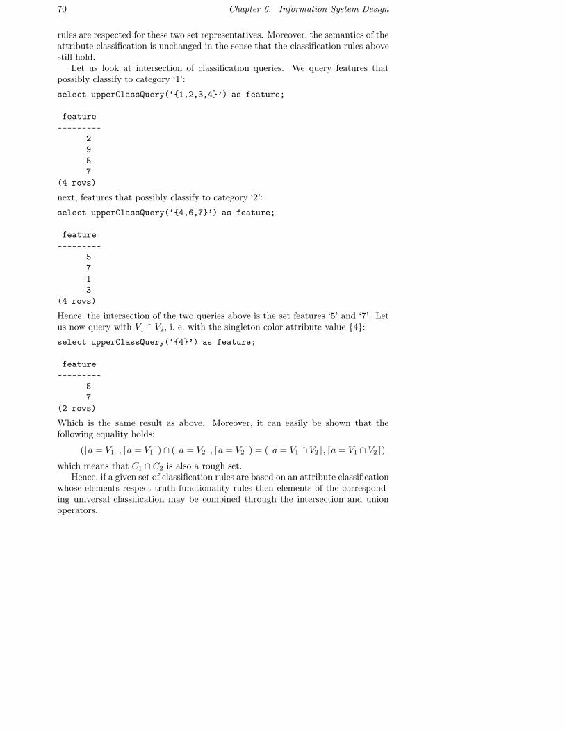
70 Chapter 6. Information System Design
rules are respected for these two set representatives. Moreover, the semantics of theattribute classification is unchanged in the sense that the classification rules abovestill hold.
Let us look at intersection of classification queries. We query features thatpossibly classify to category ‘1’:
select upperClassQuery(‘{1,2,3,4}’) as feature;
feature---------
2957
(4 rows)
next, features that possibly classify to category ‘2’:
select upperClassQuery(‘{4,6,7}’) as feature;
feature---------
5713
(4 rows)
Hence, the intersection of the two queries above is the set features ‘5’ and ‘7’. Letus now query with V1 ∩ V2, i. e. with the singleton color attribute value {4}:select upperClassQuery(‘{4}’) as feature;
feature---------
57
(2 rows)
Which is the same result as above. Moreover, it can easily be shown that thefollowing equality holds:
(�a = V1�, �a = V1�) ∩ (�a = V2�, �a = V2�) = (�a = V1 ∩ V2�, �a = V1 ∩ V2�)which means that C1 ∩ C2 is also a rough set.
Hence, if a given set of classification rules are based on an attribute classificationwhose elements respect truth-functionality rules then elements of the correspond-ing universal classification may be combined through the intersection and unionoperators.
6.6. Conclusion 71
6.6 ConclusionWe have shown how to represent approximation spaces in the relational model andwe have introduced approximate queries. We have shown how approximate queriesare used in universal classifications and we have discussed how truth-functionalityaffects the queries to the information system. The experiments performed on at-tribute classifications of our running example have confirmed that we can arrive attruth-functional operations provided that we put some restrictions on the elementsof the classification.
It is relatively easy to add fuzzy capabilities to our information system. Eachelement of the information system may have a membership value to some fuzzyset X . This can be represented by a corresponding attribute in the relationaltable. The operators µX and µX are then implemented such that they return theminimum, respectively maximum, of the membership values of a given equivalenceclass.
Note that the implementation proposed here is entirely based on the standardrelational algebra supported by most relational database systems. There may beanother possible approach that is worthwhile investigating which is to implementthe information system on top of a relational algebra that supports rough set tech-nics. The idea of extending the relational algebra to support rough set technics hasbeen presented by Beaubouef et al. in [BPB95].
The ability to store spatial data has not been implemented in the informationsystem presented here. In Chapter 7 we present an earlier implementation that hasbeen integrated into the AMOS II system [RJK00] to store spatial data. Porting thecodes developed here to AMOS II is relatively easy when the necessary relationaloperators such as union and intersection are made available in the AMOS II system.

72
Chapter 7
Experiments
Michael F. Worboys states in [Wor94]: “it is the applications which are the life-bloodof the field and give rationale to its more basic research.”
We demonstrate the viability of the model developed in this thesis by presentingsome real-life experiments.
Our implementation AMORose is presented in Section 7.1. In section 7.2we present the rough classification analysis that was performed in our joint pa-pers [AKO98, AKO00]. Section 7.3 presents the experiment on rough fuzzy classi-fications that has been presented in [AKO03].
7.1 Implementation Details
To implement our spatial information system we use the ROSE (Robust System Ex-tension) library, a library of spatial operators developed by Güting et al. in [GDS95,GS93, GS95, Sch95]. This library has been fully integrated in an object-relationaldatabase system AMOS II (Active Mediator Object System). Detailed descriptionsof the AMOS II system may be found in [FR98, RJK00] and [FJR+99, Ris99]. Thisway, it is possible to manipulate geometric data through AMOSQL, the AMOSSQL-like relational query language.
We have integrated spatial uncertainty capabilities in our system AMORose,see [Ouk01] for a detailed presentation. Spatial uncertainty has been realizedthrough our extension of the ROSE library called Rough ROSE [Ouk01].
7.2 An Example with Rough Classification
The goal of our experiment was to use the idea of rough classification to comparetwo vegetation maps, covering the same area of 1.8 by 2.3 square kilometers inStockholm County, just north of Stockholm. The two maps had been produced for
73
74 Chapter 7. Experiments
nature preservation tasks and different classification schemes were used to delineatevegetation categories on a categorical map sheet in 1:15000 scale.
In the experiment we considered the two layers as two different representationsof the same area. We started out with two vegetation maps which provided twocrisp vegetation classification layers called ‘veg9’ and ‘veg35’. Building on veget-ation concepts that were introduced by Påhlsson in [Påh72], ‘veg9’ was classifiedusing moisture and nutrient status as classification basis, giving nine different ve-getation classes for the experiment area. The vegetation map ‘veg35’ used a Nordicclassification system described by Påhlsson in [Påh95], giving 35 different vegeta-tion classes for the experiment area. The class descriptions are given in [AKO00].To compare the two, we needed to reclassify one of them; for obvious reasons, wehave chosen ‘veg35’.
Reclassification of ‘veg35’ into ‘veg9’ would be a straightforward task if a one-to-one or many-to-one correspondence between the two classification systems existed.As this is not the case, we used the idea of rough classification to represent the un-certainty in the reclassification operation. Rules to reclassify from the classificationsystem given by Påhlsson [Påh95] to the one given by Påhlsson [Påh72] were con-structed using both the guidelines given in [Påh95] and our own knowledge aboutthe association between the different vegetation classes. These classification rulesare given in [AKO00]. Note that here we use spatial uncertainty to represent thereclassification of ‘veg35’ into the nine classes of ‘veg9’.
Figure 7.2 outlines the analysis described above. In the figure, single boxesrepresent crisp classifications and double boxes represent rough classifications.
The purpose of the analysis below is to compute the overall accuracy of ‘veg9’and ‘veg35’ which has been derived in [AKO98, AKO03].
The first step in the analysis is to populate the spatial database. We omit thecode for populating the database. Each layer type ‘veg35’ and ‘veg9’ correspondsto a relation in our database. Each of them consist of a set of non-overlappingpolygons, so each can be viewed as a tessellation. The Layer ‘veg35’, denotedveg35 in the AMOSQL code below, is a subtype of layer,
create type veg35 subtype of layer;
The layers veg35 and veg9 cover exactly the same area of size total_area whichis computed as follows:
set :total_area =select sumagg(select area(reg(v35)) from veg35 v35);
The sumagg AMOSQL operator above is the sum aggregation operator on a bag ofnumbers.
The second step of the analysis is to create a relation that will represent roughclassifications:
create type classification properties (class integer key,rreg rregions)

7.2. An Example with Rough Classification 75
veg35
Rough classification
Crisp classification
Reclassification stage
Overlay
veg9
rveg9rveg35
In a rough classification the key attribute class uniquely identifies a given class. InAMORose, spatial uncertainty is represented through objects of type rough regionsrregions. Because of spatial uncertainty, rough regions may have parts that belongto more than one class.
There are two rough classifications:
create type rveg35 subtype of classification;create type rveg9 subtype of classification;
Note that ‘rveg9’ is the reference crisp classification and is a particular case of roughclassification.
The reclassification rules from the classification scheme of ‘veg35’ to the classi-fication scheme of ‘veg9’ are of the form a −→ i ∨ j. This rule means that a classa in the classification scheme of ‘veg35’ is either of attribute i or attribute j in theclassification scheme of ‘veg9’.
The classification ‘rveg35’ represents the reclassification of ‘veg35’ into the clas-sification scheme of ‘veg9’.
76 Chapter 7. Experiments
Once ‘rveg35’ and ‘rveg9’ have been populated through reclassification, we com-pute the overall accuracy of ‘rveg35’ compared to ‘rveg9’:
set :max_area = select sumagg(select Maxarea(Intersection(reg(v35), reg(v9)))
from rveg35 v35, rveg9 v9where class(v35) = class(v9));
The code above computes the area of the overlay of matching upper approximationsof ‘rveg35’ and ‘rveg9’,
set :min_area = select sumagg(select Minarea(Intersection(reg(v35), reg(v9)))
from rveg35 v35, rveg9 v9where class(v35) = class(v9));
computes the area of the overlay of matching lower approximations of ‘rveg35’ and‘rveg9’. The maximum overall accuracy is given by:
set :max_accuracy = :max_area/:total_area;
The minimum overall accuracy is given by:
set :min_accuracy = :min_area/:total_area;
Finally, the overall accuracy of ‘rveg35’ compared to the reference classification‘rveg9’ is the interval:
[min_accuracy, max_accuracy] = [0.039, 0.461]
This interval means that the overall accuracy of ‘rveg35’ is at least ‘min_accuracy’and at most ‘max_accuracy’.
7.3 Rough Fuzzy ExperimentThe experiment presented here has been described in our joint paper [AKO03] inwhich we demonstrate the viability of rough fuzzy classification. The raw data usedhere is the same as in Section 7.2 above, however, some other classification schemesare considered. Moreover, this experiment was carried out using different software.
The purpose of the experiment is to compare two vegetation maps ‘veg3’ and‘veg35’, shown in figure 7.1. These maps were taken from two separate investiga-tions covering the same area [ELP71, AW90] and have been produced for naturepreservation tasks. However, ‘veg3’ and ‘veg35’ use different vegetation classific-ation schemes. The map ‘veg3’, see Figure 7.1(a), uses 3 classes: wet, mesic anddry vegetation. ‘veg35’, on the other hand, uses 35 classes, see Figure 7.1(b). Both‘veg3’ and ‘veg35’ were digitized by scanning and segmentation into two GIS rasterimages with pixel values representing vegetation class labels. Data entry and all
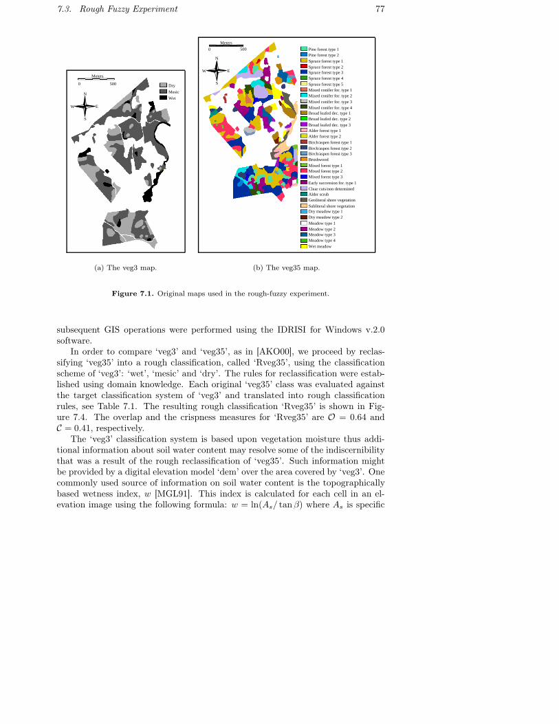
7.3. Rough Fuzzy Experiment 77
500
Mesic
Wet
0
Meters
Dry
W
S
E
N
(a) The veg3 map.
Early succession for. type 1Clear cuts/non determined
Subliteral shore vegetation
Spruce forest type 3Spruce forest type 4
Spruce forest type 5
Spruce forest type 2Spruce forest type 1
Pine forest type 2Pine forest type 1
Broad leafed dec. type 1Broad leafed dec. type 2
0 500
Meters
Dry meadow type 1Dry meadow type 2
Meadow type 1Meadow type 2
Wet meadow
Meadow type 4Meadow type 3
Mixed forest type 2Mixed forest type 3
Geoliteral shore vegetation
Mixed forest type 1
Broad leafed dec. type 3
Alder scrub
Alder forest type 1Alder forest type 2
Birch/aspen forest type 1Birch/aspen forest type 2
BrushwoodBirch/aspen forest type 3
Mixed conifer for. type 1Mixed conifer for. type 2
Mixed conifer for. type 3Mixed conifer for. type 4
S
E
N
W
(b) The veg35 map.
Figure 7.1. Original maps used in the rough-fuzzy experiment.
subsequent GIS operations were performed using the IDRISI for Windows v.2.0software.
In order to compare ‘veg3’ and ‘veg35’, as in [AKO00], we proceed by reclas-sifying ‘veg35’ into a rough classification, called ‘Rveg35’, using the classificationscheme of ‘veg3’: ‘wet’, ‘mesic’ and ‘dry’. The rules for reclassification were estab-lished using domain knowledge. Each original ‘veg35’ class was evaluated againstthe target classification system of ‘veg3’ and translated into rough classificationrules, see Table 7.1. The resulting rough classification ‘Rveg35’ is shown in Fig-ure 7.4. The overlap and the crispness measures for ‘Rveg35’ are O = 0.64 andC = 0.41, respectively.
The ‘veg3’ classification system is based upon vegetation moisture thus addi-tional information about soil water content may resolve some of the indiscernibilitythat was a result of the rough reclassification of ‘veg35’. Such information mightbe provided by a digital elevation model ‘dem’ over the area covered by ‘veg3’. Onecommonly used source of information on soil water content is the topographicallybased wetness index, w [MGL91]. This index is calculated for each cell in an el-evation image using the following formula: w = ln(As/ tanβ) where As is specific
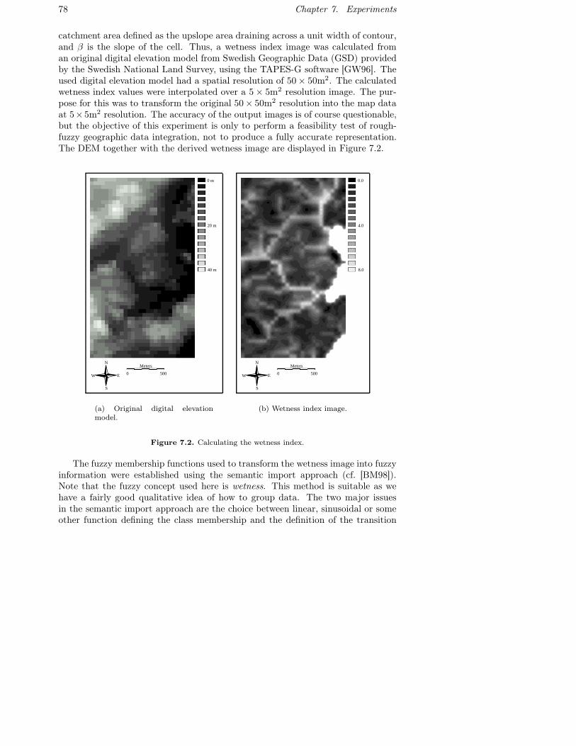
78 Chapter 7. Experiments
catchment area defined as the upslope area draining across a unit width of contour,and β is the slope of the cell. Thus, a wetness index image was calculated froman original digital elevation model from Swedish Geographic Data (GSD) providedby the Swedish National Land Survey, using the TAPES-G software [GW96]. Theused digital elevation model had a spatial resolution of 50 × 50m2. The calculatedwetness index values were interpolated over a 5 × 5m2 resolution image. The pur-pose for this was to transform the original 50× 50m2 resolution into the map dataat 5×5m2 resolution. The accuracy of the output images is of course questionable,but the objective of this experiment is only to perform a feasibility test of rough-fuzzy geographic data integration, not to produce a fully accurate representation.The DEM together with the derived wetness image are displayed in Figure 7.2.
5000
Meters
W E
S
N
0 m
20 m
40 m
(a) Original digital elevationmodel.
5000
Meters
W E
S
N
0.0
4.0
8.0
(b) Wetness index image.
Figure 7.2. Calculating the wetness index.
The fuzzy membership functions used to transform the wetness image into fuzzyinformation were established using the semantic import approach (cf. [BM98]).Note that the fuzzy concept used here is wetness. This method is suitable as wehave a fairly good qualitative idea of how to group data. The two major issuesin the semantic import approach are the choice between linear, sinusoidal or someother function defining the class membership and the definition of the transition
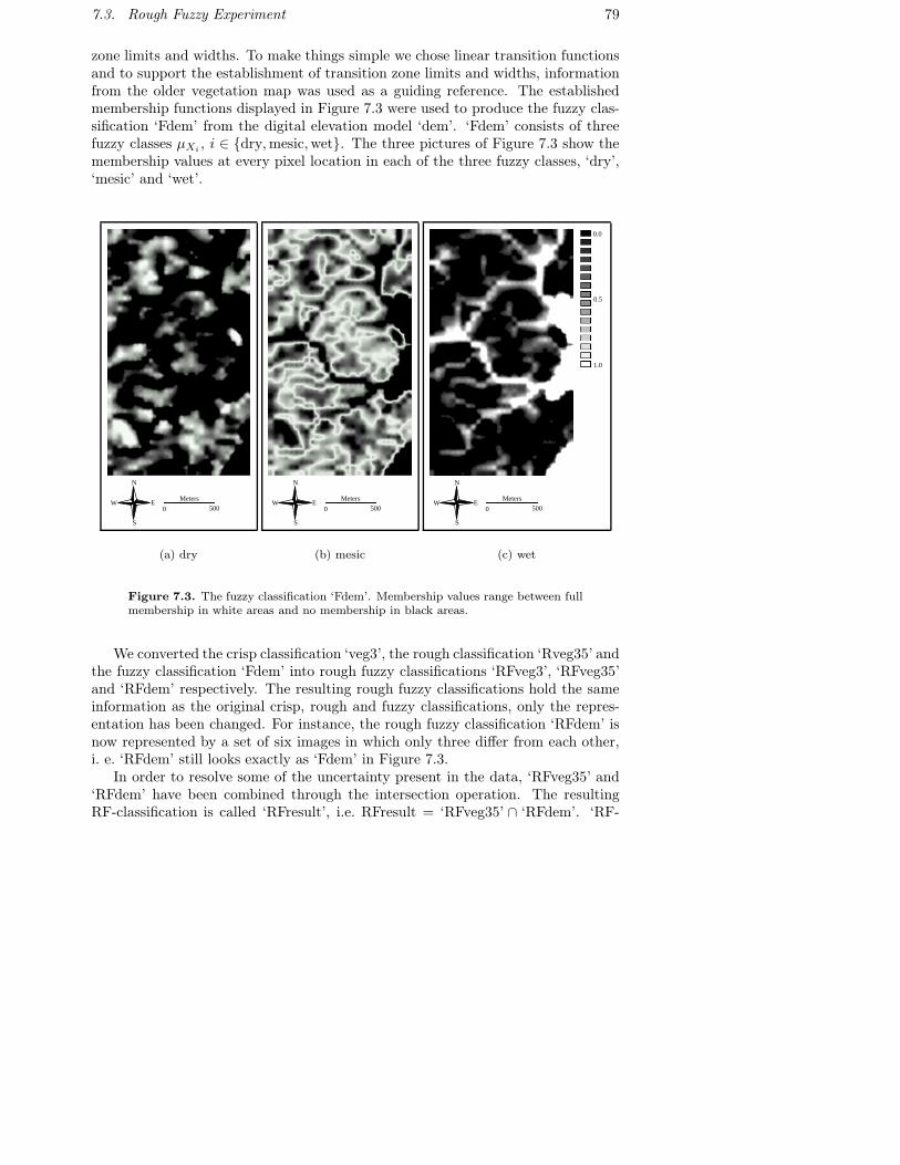
7.3. Rough Fuzzy Experiment 79
zone limits and widths. To make things simple we chose linear transition functionsand to support the establishment of transition zone limits and widths, informationfrom the older vegetation map was used as a guiding reference. The establishedmembership functions displayed in Figure 7.3 were used to produce the fuzzy clas-sification ‘Fdem’ from the digital elevation model ‘dem’. ‘Fdem’ consists of threefuzzy classes µXi , i ∈ {dry, mesic, wet}. The three pictures of Figure 7.3 show themembership values at every pixel location in each of the three fuzzy classes, ‘dry’,‘mesic’ and ‘wet’.
N
E
S
0 500
MetersW
(a) dry
N
E
S
0 500
MetersW
(b) mesic
1.0
0.5
0.0
W
S
0 500
MetersE
N
(c) wet
Figure 7.3. The fuzzy classification ‘Fdem’. Membership values range between fullmembership in white areas and no membership in black areas.
We converted the crisp classification ‘veg3’, the rough classification ‘Rveg35’ andthe fuzzy classification ‘Fdem’ into rough fuzzy classifications ‘RFveg3’, ‘RFveg35’and ‘RFdem’ respectively. The resulting rough fuzzy classifications hold the sameinformation as the original crisp, rough and fuzzy classifications, only the repres-entation has been changed. For instance, the rough fuzzy classification ‘RFdem’ isnow represented by a set of six images in which only three differ from each other,i. e. ‘RFdem’ still looks exactly as ‘Fdem’ in Figure 7.3.
In order to resolve some of the uncertainty present in the data, ‘RFveg35’ and‘RFdem’ have been combined through the intersection operation. The resultingRF-classification is called ‘RFresult’, i.e. RFresult = ‘RFveg35’ ∩ ‘RFdem’. ‘RF-
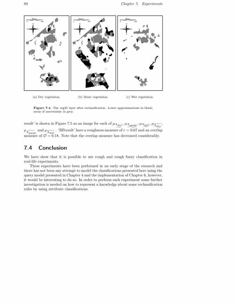
80 Chapter 7. Experiments
N
E
S
0 500
Meters
W
(a) Dry vegetation.
N
E
S
0 500
Meters
W
(b) Mesic vegetation.
N
E
S
0 500
Meters
W
(c) Wet vegetation.
Figure 7.4. The veg35 layer after reclassification. Lower approximations in black;areas of uncertainty in grey.
result’ is shown in Figure 7.5 as an image for each of µXdry˜, µXmesic
˜, µXwet˜ , µ
Xdry,
µXmesic
and µXwet
. ‘RFresult’ have a roughness measure of r = 0.67 and an overlapmeasure of O = 0.18. Note that the overlap measure has decreased considerably.
7.4 ConclusionWe have show that it is possible to use rough and rough fuzzy classification inreal-life experiments.
These experiments have been performed in an early stage of the research andthere has not been any attempt to model the classifications presented here using thequery model presented in Chapter 4 and the implementation of Chapter 6, however,it would be interesting to do so. In order to perform such experiment some furtherinvestigation is needed on how to represent a knowledge about some reclassificationrules by using attribute classifications.
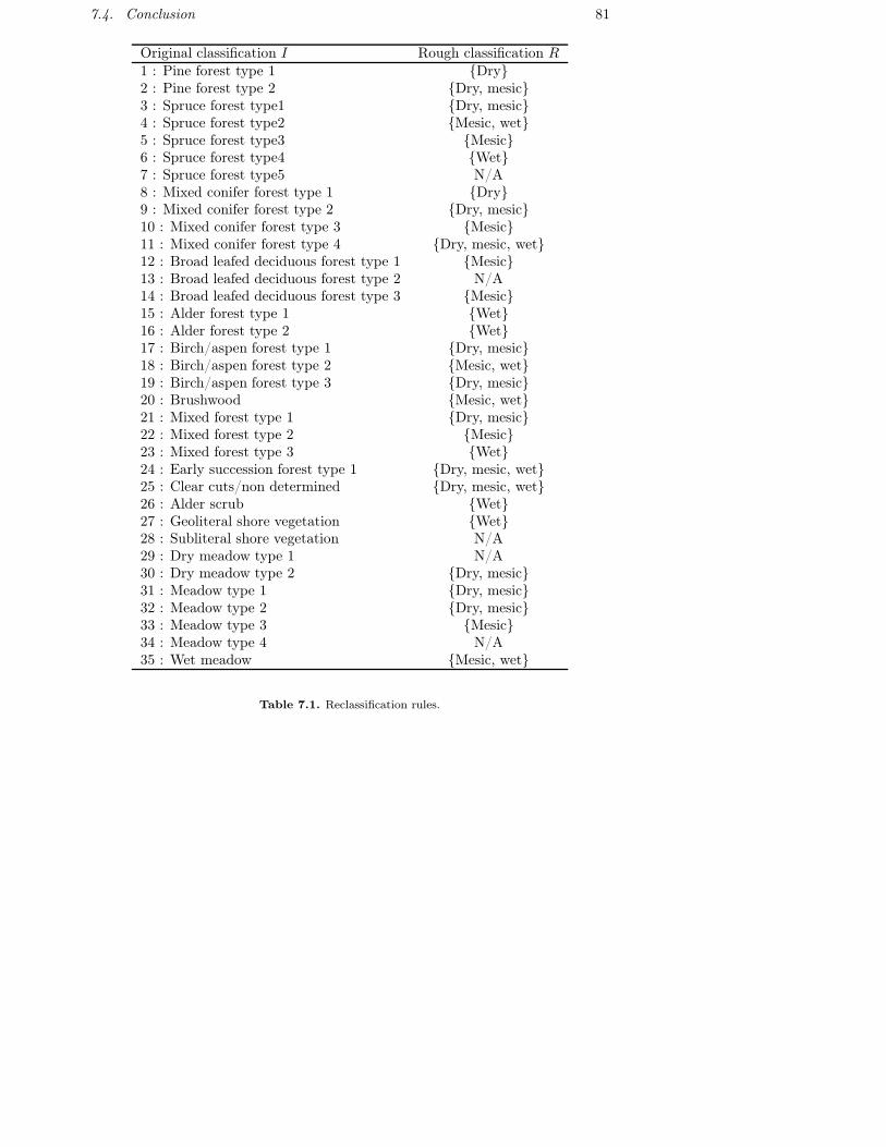
7.4. Conclusion 81
Original classification I Rough classification R1 : Pine forest type 1 {Dry}2 : Pine forest type 2 {Dry, mesic}3 : Spruce forest type1 {Dry, mesic}4 : Spruce forest type2 {Mesic, wet}5 : Spruce forest type3 {Mesic}6 : Spruce forest type4 {Wet}7 : Spruce forest type5 N/A8 : Mixed conifer forest type 1 {Dry}9 : Mixed conifer forest type 2 {Dry, mesic}10 : Mixed conifer forest type 3 {Mesic}11 : Mixed conifer forest type 4 {Dry, mesic, wet}12 : Broad leafed deciduous forest type 1 {Mesic}13 : Broad leafed deciduous forest type 2 N/A14 : Broad leafed deciduous forest type 3 {Mesic}15 : Alder forest type 1 {Wet}16 : Alder forest type 2 {Wet}17 : Birch/aspen forest type 1 {Dry, mesic}18 : Birch/aspen forest type 2 {Mesic, wet}19 : Birch/aspen forest type 3 {Dry, mesic}20 : Brushwood {Mesic, wet}21 : Mixed forest type 1 {Dry, mesic}22 : Mixed forest type 2 {Mesic}23 : Mixed forest type 3 {Wet}24 : Early succession forest type 1 {Dry, mesic, wet}25 : Clear cuts/non determined {Dry, mesic, wet}26 : Alder scrub {Wet}27 : Geoliteral shore vegetation {Wet}28 : Subliteral shore vegetation N/A29 : Dry meadow type 1 N/A30 : Dry meadow type 2 {Dry, mesic}31 : Meadow type 1 {Dry, mesic}32 : Meadow type 2 {Dry, mesic}33 : Meadow type 3 {Mesic}34 : Meadow type 4 N/A35 : Wet meadow {Mesic, wet}
Table 7.1. Reclassification rules.
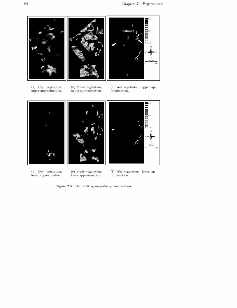
82 Chapter 7. Experiments
(a) Dry vegetation;upper approximation.
(b) Mesic vegetation;upper approximation.
0.5
0.0
1.0
W
S
0
Meters
500
E
N
(c) Wet vegetation; upper ap-proximation.
(d) Dry vegetation;lower approximation.
(e) Mesic vegetation;lower approximation.
0.5
0.0
1.0
W
S
0
Meters
500
E
N
(f) Wet vegetation; lower ap-proximation.
Figure 7.5. The resulting rough-fuzzy classification.
Chapter 8
Conclusion
We have presented a theoretical model for a language that supports queries bymeans of uncertain descriptions. This model has also been implemented in anSQL-based relational query language to demonstrate the feasibility of the idea. Wehave shown how to define uncertain classifications using our uncertain-query lan-guage and we have developed some measures to assess accuracies of classifications.Finally, we have shown the viability of uncertain classifications by performing someexperiments.
One of the main contributions of this thesis is in the area of classifications.Based on rough sets and fuzzy sets, we have given an underlying theory to explainhow classifications may be performed.
Assume for instance that you are interested in classifying a certain area into’forest’ and ’non-forest’ classes. This classification is often uncertain as it may notbe easy to draw a boundary that sharply divides forest and non-forest betweentwo distinct areas. Instead, one may be able to draw a sharp boundary somewherebetween the perimeter of an area that is certainly forest and that of an area which iscertainly not forest. Hence, we arrive at a classification with two boundaries whichreminds us of a rough set. However, the equivalence relation is not known in thiscase. This thesis proposes a solution to this issue by using approximate queries.In our model, one may exhibit the equivalence relation by querying an informationsystem by means of uncertain descriptions.
The classifications that are presented in this thesis are based on informationsystems whose elements have some particular attribute values. The particularityof the attribute values in question is that they are approximated by at most oneequivalence class in the corresponding approximation space. Note that in this thesiswe have introduced the concept of single-granular information systems to refer tothis type of information system. This has been done to simplify the discourse.Nevertheless, further research is needed to find other types of classifications thatare based on more general information systems. This may require taking intoconsideration the different interpretations of multi-valued attributes.
83

84 Chapter 8. Conclusion
We conjecture that there are new opportunities for query optimization in data-base systems that implement uncertain queries. Query optimization is known tobe an NP-hard problem [IK84]. The same complexity holds for distributed queryoptimization [ÖV99], i. e. for optimizing queries that are executed on different sites.This latter case of query optimization is especially interesting to study in conjunc-tion with approximate queries. The reason is that the heuristics used in producinga near optimal query plan often takes total communication cost into account. Oneof the particularities of rough sets is that they can be used to simplify data bydescribing them with an upper and a lower approximation. By transmitting onlylower and upper approximations of queries, one may minimize transmission costs.This may be achieved by transmitting only names of equivalence classes.
References
[AKO98] O. Ahlqvist, J. Keukelaar, and K. Oukbir. Using rough classification torepresent uncertainty in spatial data. In P. Firns, editor, Proceedings ofthe SIRC Colloquium, pages 1–9, 1998.
[AKO00] O. Ahlqvist, J. Keukelaar, and K. Oukbir. Rough classification andaccuracy assessment. International Journal of Geographical InformationScience, 14(5):475–496, 2000.
[AKO03] O. Ahlqvist, J. Keukelaar, and K. Oukbir. Rough and fuzzy geograph-ical data integration. International Journal of Geographical InformationScience, 17(3):223–234, 2003.
[AW90] O. Ahlqvist and P. Wiborn. Tranviks Naturreservat – Naturinventeringmed förslag till skötselplan. Norrtälje Kommun, 1990. In Swedish.
[BM98] P. A. Burrough and R. A. McDonnell. Principles of Geographical In-formation Systems. Oxford University Press, 1998.
[BP01] T. Beaubouef and F. Petry. Vagueness in spatial data: Rough set andegg-yolk approaches. In L. Monostori, J. Váncza, and M. Ali, editors, En-gineering of Intelligent Systems, Proceedings of IEA/AIE 2001, number2070 in Lecture Notes in Artificial Intelligence, pages 367–373, Berlin,2001. Springer-Verlag.
[BPB95] T. Beaubouef, F. Petry, and B. Buckles. Extension of the relationaldatabase and its algebra with rough set techniques. Computational In-telligence, 11(2), 1995.
[CF96] E. Clementini and P. Di Felice. An algebraic model for spatial objectswith undeterminate boundaries. In P. A. Burrough and A. U. Frank,editors, Geographic Objects with Indeterminate Boundaries, volume 2 ofGISDATA, pages 155–169, London, 1996. Taylor & Francis.
[CF97] E. Clementini and P. Di Felice. Approximate topological relations. In-ternational Journal of Approximate Reasoning, 16(2):173–204, 1997.
85
86 References
[CFvO93] E. Clementini, P. Di Felice, and P. van Oosterom. A small set of formaltopological relationships suitable for end-user interaction. In D. Abeland B. C. Ooi, editors, Third International Symposium on Large SpatialDatabases, SSD ’93, volume 692 of Lecture Notes in Computer Science,pages 277–295, Berlin, June 1993. Springer-Verlag.
[CG96] A. G. Cohn and N. M. Gotts. The ‘egg-yolk’ representation of regionswith indeterminate boundaries. In P. A. Burrough and A. U. Frank,editors, Geographic Objects with Indeterminate Boundaries, volume 2 ofGISDATA, pages 171–187, London, 1996. Taylor & Francis.
[Cod70] E. F. Codd. A relational model of data for large shared data banks.Communications of the ACM, 13(6):377–387, 1970.
[Con91] R. G. Congalton. A review of assessing the accuracy of classifications ofremotely sensed data. Remote Sensing Environment, 47:35–46, 1991.
[DG00] I. Düntsch and G. Gediga. Logical and algebraic techniques for roughset data analysis. In Lech Polkowski, Shusaku Tsumoto, and Tsau YoungLin, editors, Rough Set Methods and Applications, pages 521–544. Phys-ica Verlag, 2000.
[DGO01] I. Düntsch, G. Gediga, and E. Orlowska. Relational attribute systems.International Journal of Human-Computer Studies, 55(3):293–309, 2001.
[DP90] D. Dubois and H. Prade. Rough fuzzy sets and fuzzy rough sets. Inter-national Journal of General Systems, 17:191–209, 1990.
[DP92] D. Dubois and H. Prade. Putting rough sets and fuzzy sets together.In R. Slowinski, editor, Intelligent Decision Support – Handbook of Ad-vances and Applications of the Rough Set Theory, pages 203–232. KluwerAcademic Publishers, Dordrecht, Boston, London, 1992.
[Ege94] M. J. Egenhofer. Spatial SQL: A query and presentation language. IEEETransactions on Knowledge and Data Engineering, 6(1):86–95, 1994.
[ELP71] E. Edberg, T. Lindberg, and M. Petterson. Ängsö Nationalpark ochTranvik – vegetation och fågelfauna. Rotobeckman, Stockholm, Sweden,1971. In Swedish.
[FJR+99] S. Flodin, V. Josifovski, T. Risch, M. Sköld, and M. Werner. AMOSII User’s Guide. EDSLAB, Department of Computer Science LinköpingUniversity, August 1999.
[FR98] G. Fahl and T. Risch. AMOS2 Introduction. EDSLAB, Department ofComputer Science, Linköping University, September 1998.

References 87
[GDS95] R. H. Güting, T. De Ridder, and M. Schneider. Implementation of theROSE algebra: Efficient algorithms for realm-based spatial data types.In Lecture Notes in Computer Science, volume 951 of 4th Int. Symp. onAdvances in Spatial Databases (SSD), pages 216–239, 1995.
[Goo93] M. F. Goodchild. Data models and data quality: Problems and pro-spects. In M. F. Goodchild, B. O. Banks, and L. T. Steynaert, editors,Visualization in Geographical Information Systems, pages 141–149. JohnWiley, New York, 1993.
[Gro02] The PostgreSQL Global Development Group. PostgreSQL 7.3 Docu-mentation, 2002.
[GS93] R. H. Güting and M. Schneider. Realms: A foundation for spatial datatypes in database systems. In D. Abel and B. C. Ooi, editors, ThirdInternational Symposium on Large Spatial Databases, SSD ’93, volume692 of Lecture Notes in Computer Science, pages 14–35, Berlin, June1993. Springer-Verlag.
[GS95] R. H. Güting and M. Schneider. Realm-based spatial data types: TheROSE algebra. The VLDB Journal, 4(2):243–286, April 1995.
[GW92] M. Gehrke and E. Walker. On the structure of rough sets. Bull. PolishAcad. Sci. Math., 40:235–245, 1992.
[GW96] J. C. Gallant and J. P. Wilson. TAPES-G: A grid-based terrain analysisprogram for the environmental sciences. Computers and Geosciences,22(7):713–722, 1996.
[HS93] Z. Huang and P. Svensson. Neighborhood query and analysis with Geo-SAL, a spatial database language. In LNCS 692. Springer-Verlag, 1993.
[HSH92] Z. Huang, P. Svensson, and H. Hauska. Solving spatial analysis problemswith GeoSAL, a spatial query language. In Proceedings of the 6th Int.Working Conf. on Scientific and Statistical Database Management, 1992.
[IK84] T. Ibaraki and T. Kameda. On the optimal nesting order for computingn-relation joins. ACM Transactions on Database Systems, 9(3):482–502,1984.
[Iwi87] T. B. Iwinski. Algebraic approach to rough sets. In Bulletin of thePolish Academy of Sciences, Mathematics, volume 35, pages 673–683. A.Lasota, 1987.
[Keu02] J. Keukelaar. Topics in soft computing. PhD thesis, Royal Institute ofTechnology, Stockholm, 2002.
[Kle57] S.C. Kleene. Introduction to Metamathematics. Van Nostrand, 1957.

88 References
[KR96] M. Kryszkiewicz and H. Rybinski. Reducing information systems withuncertain attributes. In Z. W. Rás and M. Michalewicz, editors, Proceed-ings of the Ninth International Symposium on Foundations of IntelligentSystems, volume 1079 of LNAI, pages 285–294. Springer, 1996.
[LC95] F. Lehmann and A. G. Cohn. The eggyolk reliability hierarchy: Se-mantic data integration using sorts with prototypes. In Proceedings ofthe third international conference on Information and knowledge man-agement, pages 272–279. ACM Press, 1995.
[Lin01] F. Lindström. Världens dåligaste språk: tankar om språket och män-niskan. Månpocket, 2001. In Swedish.
[MGL91] I. D. Moore, R. B. Grayson, and A. R. Ladson. Digital terrain modelling:A review of hydrological, geomorphological and biological applications.Hydrologic Processes, 5(1):3–30, 1991.
[Mom01] B. Momjian. PostgreSQL: introduction and concepts. Addison-Wesley,Reading, MA, USA, 2001.
[MT99] V. W. Marek and M. Truszczyński. Contributions to the theory of roughsets. FUNDINF: Fundamenta Informaticae, 39(4):389–409, 1999.
[OKA01] K. Oukbir, J. Keukelaar, and O. Ahlqvist. Rough point set topologicalrelations. Nada Report, ref. number TRITA-NA-0111, 2001.
[Ouk97] K. Oukbir. Amorose, a realm based spatial database system. In Pro-ceedings of ScanGIS, 1997.
[Ouk01] K. Oukbir. A database query language for uncertain spatial data. De-partment of Numerical Analysis and Computer Science (Nada), KTH.Licentiate Thesis, ISBN 91-7283-134-0, 2001.
[ÖV99] M. Tamer Özsu and P. Valduriez. Principles if Distributed DatabaseSystems. Prentice Hall, second edition, 1999.
[Påh72] L. Påhlsson. Översiktlig Vegetationsinventering. Statens Naturvårdsverk,Stockholm, 1972. In Swedish.
[Påh95] L. Påhlsson. Vegetationstyper i Norden. Number 1994:665 in Tema Nord.Nordic Council of Ministers, Copenhagen, 1995. in Swedish.
[Paw82] Z. Pawlak. Rough sets. International Journal of Computer and Inform-ation Sciences, 11(5):341–356, 1982.
[Paw85] Z. Pawlak. Rough sets and fuzzy sets. Fuzzy Sets and Systems, 17(1):99–102, 1985.
References 89
[Paw91] Z. Pawlak. Rough Sets: Theoretical Aspects of Reasoning about Data.Kluwer Academic Publishers, Dordrecht, 1991.
[Paw96] Z. Pawlak. Rough sets, rough relations and rough functions. FUNDINF:Fundamenta Informaticae, 27, 1996.
[Pol02] L. Polkowski. Rough sets, mathematical foundations. In J. Kacprzyk,editor, Advances in Soft Computing, chapter 14. Physica-Verlag, 2002.
[Ris99] T. Risch. AMOS II External Interfaces. EDSLAB, Department of Com-puter Science Linköping University, April 1999.
[RJK00] T. Risch, V. Josifovski, and T. Katchaounov. AMOS II concepts. Tech-nical report, Uppsala Database Laboratory (UDBL), June 2000.
[RS01] A. J. Roy and J. G. Stell. Spatial relations between indeterminate re-gions. International Journal of Approximate Reasoning, 27(3):205–234,2001.
[SC03] S. Shekhar and S. Chawla. Spatial Databases: A Tour. Prentice Hall,2003.
[Sch95] M. Schneider. Spatial Data Types for Database Systems. PhD thesis,Fachbereich Informatik, FernUniversität Hagen, 1995.
[SW98] J. G. Stell and M. F. Worboys. Stratified map spaces. In T. Poinker andN. Chrisman, editors, Proceedings of the 8th International Symposiumon Spatial Data Handling, pages 180–189. Taylor and Francis, 1998.
[Thi98] H. Thiele. Fuzzy rough sets versus rough fuzzy sets– an interpretationand a comparative study using concepts of modal logics. Technical Re-port CI-30/98, University of Dortmund Dept. of Computer Science, 1998.
[WC01] M. F. Worboys and E. Clementini. Integration of imperfect spatial in-formation. Journal of Visual Languages and Computing, 12:61–80, 2001.
[Wor94] M. Worboys, editor. Innovations in GIS 1, chapter 3. Taylor & Francis,London, UK., 1994.
[Yao93] Y. Y. Yao. Interval-set algebra for qualitative knowledge representation.In Proc. 5th international Conference on Computing and Information,pages 370–374, 1993.
[Yao96] Y. Y. Yao. Two views of the theory of rough sets in finite universes.International Journal of Approximate Reasoning, 15:291–317, 1996.
[Yao97] Y. Y. Yao. Combination of rough and fuzzy sets based on α-level sets. InT. Y. Lin and N. Cercone, editors, Rough Sets and Data Mining: Ana-lysis for Imprecise Data, volume 104, pages 301–321. Kluwer AcademicPublishers, 1997.

90 References
[YL96] Y. Y. Yao and X. Li. Comparison of rough-set and interval-set modelsfor uncertain reasoning. FUNDINF: Fundamenta Informatica, 27, 1996.
[YWL97] Y. Y. Yao, S. K. M. Wong, and T. Y. Lin. A review of rough set models.In T. Y. Lin and N. Cercone, editors, Rough Sets and Data Mining:Analysis for Imprecise Data, pages 47–75. Kluwer Academic Publishers,Boston, 1997.
[Zad65] L. A. Zadeh. Fuzzy sets. Information and Control, 8:338–353, 1965.