Embed Size (px)
Citation preview
Indirect Inference
C. Gourieroux; A. Monfort; E. Renault
Journal of Applied Econometrics, Vol. 8, Supplement: Special Issue on Econometric InferenceUsing Simulation Techniques. (Dec., 1993), pp. S85-S118.
Stable URL:
http://links.jstor.org/sici?sici=0883-7252%28199312%298%3CS85%3AII%3E2.0.CO%3B2-7
Journal of Applied Econometrics is currently published by John Wiley & Sons.
Your use of the JSTOR archive indicates your acceptance of JSTOR's Terms and Conditions of Use, available athttp://www.jstor.org/about/terms.html. JSTOR's Terms and Conditions of Use provides, in part, that unless you have obtainedprior permission, you may not download an entire issue of a journal or multiple copies of articles, and you may use content inthe JSTOR archive only for your personal, non-commercial use.
Please contact the publisher regarding any further use of this work. Publisher contact information may be obtained athttp://www.jstor.org/journals/jwiley.html.
Each copy of any part of a JSTOR transmission must contain the same copyright notice that appears on the screen or printedpage of such transmission.
The JSTOR Archive is a trusted digital repository providing for long-term preservation and access to leading academicjournals and scholarly literature from around the world. The Archive is supported by libraries, scholarly societies, publishers,and foundations. It is an initiative of JSTOR, a not-for-profit organization with a mission to help the scholarly community takeadvantage of advances in technology. For more information regarding JSTOR, please contact [email protected].
http://www.jstor.orgSat Jan 5 12:50:08 2008
JOURNAL OF APPLIED ECONOMETRICS, VOL. 8, S85-S118 (1993)
INDIRECT INFERENCE
C. GOURIEROUX CREST and CEPREMAP, I5 bvd Gabriel-PPri, 92245 Malakoff, Cedex France
A. MONFORT CREST-ZNSEE, 15 bvd Gabriel-Phi, 92245 Malakoff, Cedex France
AND
E. RENAULT GREMAQ-ZDEZ, 75 bvd de la Marquette, 31000 Toulouse, France
SUMMARY
In this paper we present inference methods which are based on an 'incorrect' criterion, in the sense that the optimization of this criterion does not directly provide a consistent estimator of the parameter of interest. Moreover, the argument of the criterion, called the auxiliary parameter, may have a larger dimension than that of the parameter of interest. A second step, based on simulations, provides a consistent and asymptotically normal estimator of the parameter of interest. Various testing procedures are also proposed. The methods described in this paper only require that the model can be simulated, therefore they should be useful for models whose complexity rules out a direct approach. Various fields of applications are suggested (microeconometrics, finance, macroeconometrics).
1. INTRODUCTION
Econometric models often lead to complex formulations for the conditional distribution of the endogenous variables given the exogenous variables and the lagged endogenous values. These formulations may even be such that, it is impossible to efficiently estimate the parameters of interest because of the intractability of the likelihood function. The examples of such situations are numerous in the literature: discrete choice models with a large number of alternatives, job search models, description of optimal dynamic behaviours, non-linear models with random coefficients, non-linear rational expectation models, continuous-time model with stochastic volatility, factor ARCH models. In such cases, a natural procedure is to replace the likelihood function by another criterion. This criterion could be, for instance, an approximation of the exact likelihood function, or the exact likelihood function of an approximated model, but we shall see that the choice is much larger.
The aim of this paper is to show that a correct inference can be based on this 'incorrect' criterion. The main steps of the estimation method, called the indirect estimation method, are the following. First, we consider an auxiliary parameter and an estimation method for this parameter. Then this method is applied to the observations and to simulated values drawn
0883-7252/93/OSOS85-34$22.00 Received September 1992 O 1993 by John Wiley & Sons, Ltd. Revised May 1993
S86 C. GOURIEROUX, A. MONFORT AND E. RENAULT
from the true model and associated with a value 0 of the parameter of interest. Finally, 8 is calibrated in order to obtain close values for the two estimators of the auxiliary parameter. The resulting estimator of 8 has rather nice asymptotic properties when the auxiliary parameter and the criterion are well chosen and this allows for the development of a complete theory of indirect estimation. This kind of method was first proposed by Smith (1990) and the extensions described here are threefold. First, we take explicitly into account the presence of exogenous variables and we derive the modified variance-covariance matrix of the estimator. Second, we consider more general criteria for the first-step estimator of the auxiliary parameter. Third, we introduce several specification tests of the initial model and a general theory of hypotheses testing based on indirect estimation. Moreover, we show how these methods can be applied to the microeconometrics, macroeconometrics, and econometrics of finance.
In Section 2 we describe the indirect estimation method with its two steps: (1) definition and estimation of the auxiliary parameter and (2) calibration of the parameter of interest by comparison of the estimators of the auxiliary parameter computed from the observations and from simulations, respectively.
The asymptotic distributional properties of indirect estimators are given in Section 3. They depend on the retained auxiliary parameter, on the first-step estimation procedure, on the metric used to compare the two estimators, and on the number of simulated values. We discuss the optimal choice of the metric. Moreover, we show that the indirect method contains, as a special case, the simulated method of moments (SMM) (McFadden, 1989; Pakes and Pollard, 1989; Duffie and Singleton, 1989; Smith, 1993; GouriCroux and Monfort, 1993).
In Section 4 we show how indirect estimators may be used to construct specification tests. We also propose a consistency test for the estimator of the parameter of interest based on a proxy model.
In Section 5 we introduce a general test theory based on indirect estimators and we show, in particular, that the usual equivalence between the Wald test, the score test, and the test based on optimal values of the objective function remains valid despite the presence of simulations.
In Section 6 we consider a simple Monte Carlo illustration of the technique: the estimation of the parameters of a moving-average process by means of a preliminary estimation of an autoregressive representation. In this case the indirect estimation method may be seen as a way of correcting for the lag truncation effect in the AR representation. Some light on the finite sample properties of the method is obtained from this example.
In Section 7 we show how the indirect methods can be used for the estimation of the parameters appearing in stochastic differential equations. Monte Carlo results are given for the case of a geometric brownian motion and of an Ornstein-Uhlenbeck process.
In Section 8 we consider two applications to the econometrics of finance: estimation of stochastic volatility models and of factor ARCH models.
In Section 9 we describe potential applications to microeconometrics. In discrete choice models with a large number of alternatives, the log-likelihood function often contains high- dimensional integrals. To solve this problem we first exhibit a logit approximation of the c.d.f of the multivariate normal distribution. Then this approximation is used to base the indirect approach on an approximated maximum likelihood procedure.
In Section 10 we describe some examples in the domain of macroeconometrics: correction for the linearization of a non-linear model, correction for the use of the extended Kalman filter.
Section 11 concludes and the proofs are given in four appendices.
INDIRECT INFERENCE
2. INDIRECT ESTIMATION METHODS
2.1. The Model
We consider the following dynamic model:
where the x/s are observable exogenous variables whereas the u/s and the &;s are not observed. We assume that: (Al) (xt)is an homogeneous Markov process, independent of (et) (and (ut)) ; the process (et) is a white noise whose distribution GO is known, and the process (yt,xt) is stationary.
Note that the knowledge of the distribution of et is not a real assumption, in the parametric case, since ttcan always be considered as a function of a white noise with a known distribution and of a parameter which can be incorporated into 6.
The conditional probability density function (p.d.f.) of xt given its past is denoted by: fo(xt/xt-1) =fo(xt/xt-I), where xt-I= (xt-l,xt-2, ...1.
Models with processes of larger order or with reduced forms containing more than one lag in y, x, or u can be included in the previous formulation by increasing the dimension of the processes.
Under the above assumption it is possible to simulate values of yl, ...,y~ for a given initial condition zo = (yo, uo) and a given value of the parameter 8, conditionally to an observed path of the exogenous variables xo, . . .XT. This is done by drawing simulated values 2.1, ...,ET in GO, and by computing
where
Note that assumption (Al) implies that xt is a strongly exogenous process. This means that we assume that potential problems due to non-strongly exogenous variables have been solved by considering them as functions of lagged endogenous variables. It is also worth noting that models in which non-strongly exogenous variables appear have the serious drawback of not being simulable.
With such a parametric model it is theoretically possible to compute the conditional density function of yl ...YT given 20, XI ...XT, and therefore to estimate the unknown true value 00 of 8 by a conditional maximum likelihood approach. However, in practice this likelihood function may be computationally intractable. In the following subsections we describe two-step estimation methods, in which all that is required from model (1) is to be easily simulated.
2.2. The Auxiliary Parameter and its Estimator
The auxiliary parameter and its estimator are defined in the following way. We introduce a criterion which depends on the observations y: = (yl, . . .,YT), XT
1 = (XI,. . ..,XT) and on the
S88 C. GOURIEROUX, A. MONFORT AND E. RENAULT
auxiliary parameter P E B c Rq.This parameter is estimated by maximizing the criterion
Max Q T ( Y ~ , (3)xh, 0 ) PEE
We denote by DT the solution of this problem:
Let us assume that the criterion tends asymptotically (and uniformly almost certainly) to a non-stochastic limit:
lim QT(Y~, Q-(Fo, Go, 80, P) xh, P) = T+-
This limit depends on the unknown auxiliary parameter @,on the characteristics of the true distribution (i.e. the transition distribution FOof (x t ) , which is unknown), on the marginal distribution GO of (ct) (which is known), and on the true parameter of interest 80. It may also depend on the initial value 20, and equation (5) includes the assumption that the initial conditions have no asymptotic effects. Moreover, let us assume that this limit criterion is continuous in p and as a unique maximum:
We know from the usual asymptotic theory (see Gallant and White, 1988, Chapter 3) that under assumptions (Al), (A2) and (A3) the estimator 6~is a consistent estimator of the auxiliary parameter 00. It is clear that the auxiliary parameter is unknown since it depends on the unknown parameter of interest 80 as well as on the unknown transition distribution FO of the exogenous variables. Moreover, it will be useful to introduce the so-called binding function (GouriCroux and Monfort, 1992) defined by
b(F, G, 8) = Argmax Qm(F, G, 8,P) PCB
We have Po = b(Fo, Go, 80)
If the function
b(Fo, Go, .): 8 b(Fo, Go, 8) +
was known and one to one, we could deduce from DT a consistent estimator of the unknown parameter of interest 80 by considering the solution 6~of DT = ~ ( F o ,GO, BT). However, if the model contains some exogenous variables, FOis unknown and the previous approach cannot be used. ' Even for models without exogenous variables, i.e. for pure time-series models, the
'Moreover, even if FOwas known, such an approach would be generally suboptimal since it does not efficiently use the information provided by observations x i , of exogenous variables. For instance, in the case of i.i.d. random variables (x , ,y , ) , t = 1,2, ...,T and of an auxiliary parameter 0 which is estimated by an M-estimation procedure:
it is clear that this estimator satisfies &= b (I%, GT,B o ) , where PT and € T are the empirical probability distribution of x and u( = E ) . Therefore if the 'finite sample biflding function' b(&, € T , .) (see GouriCroux and Monfort, 1992) was known and one to one we could deduce from PT the exact value 00 of unknown parameters while the knowled~e of the true binding function b(F0, Go, .) and the solution of b(F0, GO, 0 ) = PT only provides a consistent estimator BT! This is the reason why the indirect estimation procedure of Bo follows the previous idea after replacement of the unknown function b(I%, GT, .) by ̂a functional estimator based on simulations of the y's. It is important to keep in mind that we try to estimate ~ ( F T , .) rather than b(F0, Go, .). In order to do this, it is better to perform only &T,
simulations of the u, associated with observed values of the x,.
INDIRECT INFERENCE S89
binding function may be difficult to compute. The second step of the estimation procedure follows the previous idea after replacement of the unknown function ~ ( F o , aGo, .) by functional estimator based on simulations of the y's. The following assumption will be necessary:
ab (A41 ~ ( F o ,Go,.) is one to one and, ae (PO,GO,80) is of full-column rank (9)
2.3. The Second Step
For a given value of 8 , we can consider H simulated paths [j!(8,zoh),t = 0, ...T I , h = 1 ...H based on independent drawings of ct, (E:, ...,E$), and on initial values zoh, h = 1 , ...H.
For each of these paths, we can also consider the optimization problem:
Max Q T ( ( Y ~ ) ~ (10)xi, P ) PCB
in which the observed values are replaced by the simulated ones. This problem has a solution:
When T tends to infinity this solution tends to a solution of the limit problem:
Max Qw(F0, Go, 8, P ) PCB
lim bhT(8,zoh) = GO,8 )~ ( F o ,T+ w
Therefore &(.,zoh) is a consistent functional estimator of b(Fo, Go, .). It is now possible to define the indirect estimator of 8. The idea is simply to calibrate the
value of 8 in order to have
close to DT.
Proposition I : An indirect estimator of 8 is defined as a solution 6?(Q) of a minimum distance problem:
where OT is a positive definite matrix converging to a deterministic positive definite matrix Q. Under assumptions ( A l ) , (A2), (A3) and (A4) the indirect estimator (?(a) is a consistent estimator of 80.
The previous approach necessitates H optimizations of the simulated criterion for each value of 8 involved in the minimization algorithm. It is possible to replace these H optimizations by only one. Let us first consider the TH values of the x variables obtained by repeating H times the values X I ...XT:
21 = X i , . . . ,?T = XT, ?T+ 1 = X i , ...,?TH = XT.
S90 C. GOURIEROUX, A. MONFORT AND E. RENAULT
Then we compute
where
and Et, t = 1, . .. ,TH are TH drawings of the white noise process (et ) . This approach is equivalent to H drawings of values 7: ...J$, with different initial values
20,ZT= (yT, GT), ...ZT(H-I) = ( y T ( ~ - iiT(~-,)). From these simulated data we may deduce a simulated criterion Q T [ ~ ~ H , jZiH,01 and the associated estimator
Proposition 2: Another version of the indirect estimator of 8 is defined as the solution of
Min (P^T - )'OT[P^T ~ H T ( ~ , Y O ) ]~ H T [ ~ , Y O ] -eeg
It is a consistent estimator of 80 under the same conditions as in proposition 1.
It will be shown in Appendix 1 that both versions of the indirect estimator have the same asymptotic properties.
This kind of estimator is considered by Smith (1990) for specific criteria based on misspecified log-likelihood functions and when no exogenous variables are present.
2.4. Numerical Aspects
It should be emphasized that the indirect estimator is obtained without evaluating the complete functions p$(., z0h) or ~ H T ( . , ZO), but only their values for the 8's appearing in the optimization algorithm. Moreover, the same simulated values t:, ...,t$, h = 1, ...H are used for all the values of 8; these values can be either stored in memory or redrawn with the same seed values.
In several applications (see Sections 7-10) the auxiliary parameter and the criterion are defined in one of the following ways. First, we can replace the initial reduced-form equation (1) by another:
yt = r*(yt-l,xt, ut, P) (13)
where r* is an approximation of r for which the conditional log-likelihood function L I*;@)may be easily derived and we take QT= (l/T)LI*;(o). Second, we can take for QT an approximation of (~/T)LT(P), where LT(P) is the exact log-likelihood function. In such cases the estimation method based on QT is an approximated log-likelihood method and the P parameter often has the same dimension as 8 (and a similar interpretation). In these important cases, the indirect estimator is independent of the choice of GT and is the solution of
This system may be solved numerically by using as initial value of 8: 8' = P~T.
INDIRECT INFERENCE S91
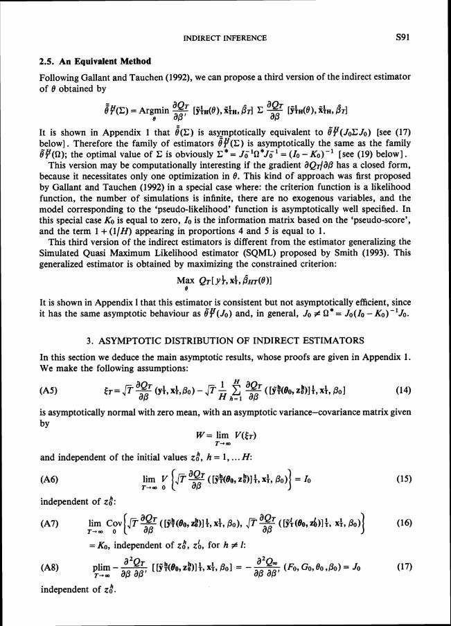
2.5. An Equivalent Method
Following Gallant and Tauchen (1992), we can propose a third version of the indirect estimator of 8 obtained by
;p(C) = ~ Q T 811 E %H, @TIArgmin -7[$H(B), %$H, [WH(~), e aP a0
It is shown in Appendix 1 that ;(c) is asy_mptotically equivalent to $?(JOCJO) [see (17) below]. Therefore the family of estimators #F(C) is asymptotically the same as the family $P(Q);the optimal value of C is obviously C * = J,T1Q*Jg' = (lo -KO)-' [see (19) below I .
This version may be computationally interesting if the gradient aQ~/a/3 has a closed form, because it necessitates only one optimization in 8. This kind of approach was first proposed by Gallant and Tauchen (1992) in a special case where: the criterion function is a likelihood function, the number of simulations is infinite, there are no exogenous variables, and the model corresponding to the 'pseudo-likelihood' function is asymptotically well specified. In this special case KO is equal to zero, I 0 is the information matrix based on the 'pseudo-score', and the term 1 + (l/H) appearing in proportions 4 and 5 is equal to 1.
This third version of the indirect estimators is different from the estimator generalizing the Simulated Quasi Maximum Likelihood estimator (SQML) proposed by Smith (1993). This generalized estimator is obtained by maximizing the constrained criterion:
Max QT [Y A x:, BHT(~)Ie
It is shown in Appendix 1 that this estimator is consistent but not asymptotically efficient, since it has the same asymptotic behaviour as &;(JO) and, in general, JO# Q*= Jo(Io -KO)-'JO.
3. ASYMPTOTIC DISTRIBUTION OF INDIRECT ESTIMATORS
In this section we deduce the main asymptotic results, whose proofs are given in Appendix 1. We make the following assumptions:
is asymptotically normal with zero mean, with an asymptotic variance-covariance matrix given by
W = lim V([T) T+ w
and independent of the initial values zoh, h = 1, .. . H:
independent of zoh:
=KO, independent of zoh, zb, for h # I:
plim --a'Qr [ [j.?(80, zt)l:, xi, 601= --(Fo, G0,80,h) = JO T+m ap apt 80 aol
independent of zoh.
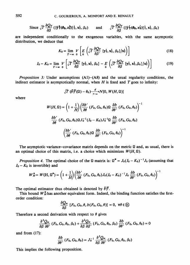
C. GOURIEROUX, A. MONFORT AND E. RENAULT
([Y!(BO, zDII, $, Po) ~ Q TSince JTQT and -([?k(Bo, zb)lI, xi, Bo) a6 a@
are independent conditionally to the exogenous variables, with the same asymptotic distribution, we deduce that
Proposition 3: Under assumptions (A1)-(A8) and the usual regularity conditions, the indirect estimator is asymptotically normal, when H is fixed and T goes to infinity:
d (8F(n) -60 )-NO, W(H, Q)IT-m
where
ab(Fo, Go, Bo)Q --;(Fo, Go, do) ae
abf ab -(Fo, Go, Oo)QJol(Io -K~)JC'Q--;(Fo, Go, 00) ae ae
aba b f (Fo, Go, Bo)Q -7(Fo, Go, 00) ae
The asymptotic variance-covariance matrix depends on the metric Q and, as usual, there is an optimal choice of this matrix, i.e. a choice which minimizes W(H, Q).
Proposition 4. The optimal choice of the Q matrix is: Q* = Jo(I0 -KO)-'Jo (assuming that 10-KO is invertible) and
The optimal estimator thus obtained is denoted by 8F. This bound ~ ; " r h a s another equivalent form. Indeed, the binding function satisfies the first-
order condition:
de- [Fo, GO, 0, b(F0, Go, 8)] = 0, \18 €0a@ Therefore a second derivation with respect to 8 gives
ab (Fo,Go,6'o,h)+- (Fo, Go,Bo, Po) 7(Fo, Go, 00) = 0
ap ae a@apf ae and from (17):
ab -ael (Fo,Go,Bo)= JC -ap aef (Fo, Go, 00,Bo)
This implies the following proposition.
INDIRECT INFERENCE
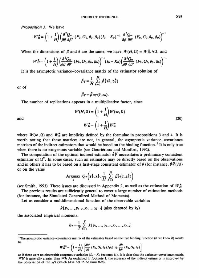
Proposition 5. We have
When the dimensions of 0 and 0 are the same, we have W(H, Q) = w;, VQ, and
It is the asymptotic variance-covariance matrix of the estimator solution of
The number of replications appears in a multiplicative factor, since
and
where W(oo, Q) and W: are implicity defined by the formulae in propositions 3 and 4. It is worth noting that these matrices are not, in general, the asymptotic variance-covariance matrices of the indirect estimators that would be based on the binding function. It is only true when there is no exogenous variable (see GouriCroux and Monfort, 1992).
The computation of the optimal indirect estimator 8F necessitates a preliminary consistent estimator of Q*. In some cases, such an estimator may be directly based on the observations and in others it has to be based on a first-stage consistent estimator of 8 (for instance, 8?(1d) or on the value
Argmax QT (Y:, x i , -l CH M e , z t ) 18 H h = 1
(see Smith, 1993). These issues are discussed in Appendix 2, as well as the estimation of w;. The previous results are sufficiently general to cover a large number of estimation methods
(for instance, the Simulated Generalized Method of Moments). Let us consider a multidimensional function of the observable variables
k [yt,...,yt-,, xt, ...xt-,I (also denoted by kt)
the associated empirical moments:
'The asymptotic variance-covariance matrix of the estimator based on the true binding function (if we knew it) would
as if there were no observable exogenous variables (10 -KO becomes 10). It is clear that the variance-covariance matrix Ws* is generally greater than Wk. As explained in footnote 1, the accuracy of the indirect estimator is improved by the observation of the xr's (which have not to be simulatedj.
s94 C. GOURIEROUX, A. MONFORT AND E. RENAULT
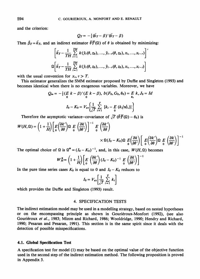
and the criterion:
QT= - ) ( k ~ - P ) ' ( ~ T - P)
Then b ~ = k ~ , and an indirect estimator @F(Q) of 8 is obtained by minimizing:
with the usual convention for x,, T > T. This estimator generalizes the SMM estimator proposed by Duffie and Singleton (1993) and
becomes identical when there is no exogenous variables. Moreover, we have
Qm= - ) (E k - P) '(E k - p), b(F0, Go, 00) = E k, J o = Id 0 0 00
0 1 Therefore the asymptotic variance-covariance of (8Tn(~)- 00) is
W(H, " +;) (1= [:(%)a f ($)I f (%)
The optimal choice of Q is Q* = (10-KO)-', and, in this case, W(H, Q) becomes
w;= (I+;)[; ( % ) ( I ~ - K ~ ) - ~ EO
In the pure time series cases KO is equal to 0 and IO-KO reduces to T
which provides the Duffie and Singleton (1993) result.
4. SPECIFICATION TESTS
The indirect estimation model may be used in a modelling strategy, based on nested hypotheses or on the encompassing principle as shown in GouriCroux-Monfort (1992), (see also GouriCroux et al., 1983; Mizon and Richard, 1986; Wooldridge, 1990; Hendry and Richard, 1990; Pesaran and Pesaran, 1991). This section is in the same spirit since it deals with the detection of possible misspecifications.
4.1. Global Specification Test
A specification test for model (1) may be based on the optimal value of the objective function used in the second step of the indirect estimation method. The following proposition is proved in Appendix 3.
INDIRECT INFERENCE
Proposition 6: The statistics:
and -ET=- TH Min [fir -$HT(~,ZO)]18: [f l~- FHT(~, ZO)]
1+ H eeg where d: is a consistent estimator of Cl*, are asymptotically distributed as a chi-square with q -p degrees of freedom, where q = dim 0, p =dim 8, when the reduced-form equation (1) is well specified. Specification tests of asymptotic level CY are associated with the critical regions:
4.2. A Consistency Test for the Proxy Model
When the initial complex model is replaced by another, in which the parameters 0 have the same dimension as 8 and similar interpretations, it is natural to see if the proxy model is really a good approximation of the initial one. For this purpose it is useful to compare:
(1) The estimator 6~of 0 computed from the observations; (2) The estimator BHT(~~T, as the value ZO) computed from the simulations with the value f i ~
of 8 parameter.
Such an approach does not require the knowledge of the observations, but simply the forms of the two models and the knowledge of the estimation under the proxy model. It is a tool for checking a posteriori the accuracy of the approximation.
The implicit null hypothesis is defined by the constraint
b(Fo, Go, 80) = b(Fo, Go, b(Fo, Go, 80)) " 80=b(Fo, Go, 80) (because of the injectivity of b) e 6~consistent estimator of 80
This implicit null hypothesis appears as a constraint on 80 (see next section), where the function b defining the constraint has to be estimated. If, for instance, the auxiliary parameter is estimated by a maximum likelihood method on the proxy model, i.e. by a pseudo-maximum likelihood method, we are simply testing for the hypothesis of consistency of the PML estimator.
The asymptotic distribution of ST [BT- BHT(~~T,zo)] Otheris derived in Appendix 3. specifications tests based on different criteria could be proposed (see GouriCroux et a/., 1992).
5. INDIRECT TESTS OF HYPOTHESES ON THE PARAMETER OF INTEREST
The indirect estimation approach can be used to test hypotheses on parameter 8. We assume that the parameter 8 is partitioned into
where 81 and 82 have dimensions pl and p2, respectively. We consider the null hypothesis Ho = (81 =0).
Despite the use of simulated values the usual equivalence between the Wald test, the score
S96 C. GOURIEROUX, A . MONFORT AND E. RENAULT
test, and the test based on the comparison of the constrained and unconstrained values of the objective function used in the second step remains valid, as shown in Appendix 4.
To define these tests we have to introduce the optimal unconstrained indirect estimator:
and the optimal constrained indirect estimator obtained by optimizing the criterion submitted to 81 = 0.This estimator is denoted by
The Wald statistic is defined as
ETW = T(@T)' w?-'(~!T)
where W? is a consistent estimator of the asymptotic covariance-variance matrix of ~YT. The score statistic is defined from the gradient of the objective function with respect to 81
evaluated at the unconstrained estimator. This gradient is given by:
and the test statistic is
#ST = Tg+Aw?%, (23)
Finally, we can introduce the difference between the optimal values of the objective fucntion:
C? = [~BT-BT(8 gH)l '0 ;[fir -PHT(8 gH)l l + H
--TH [fir -PHT(~?)I'0: [fir- PHT(~?)I (24)l + H
Proposition 7. The test statistics #T, ##, and #$are asymptotically equivalent under the null hypothesis, and have the common distribution X 2 (PI).
Proof. See Appendix 4. As usual, the test based on the optimal values of the objective function requires both
constrained and unconstrained estimation (and simulations). In constrast, the Wald or score test procedures only necessitate, respectively, unconstrained and constrained estimations (and simulations).
6. A SIMPLE EXAMPLE
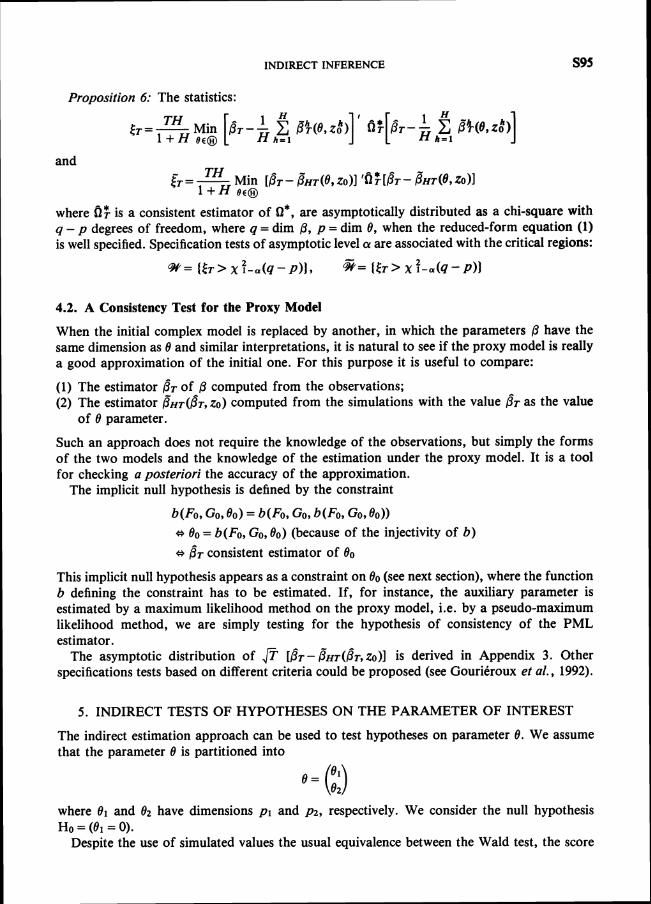
In this section we consider the estimation of the parameter 8 of a Gaussian moving-average process:
Y ~ = E ~ - ~ E ~ - It = 1, ...,T
where the true value of 8 is 0-5 and the true variance of ct is 1. The aim is to compare the
INDIRECT INFERENCE
Figure 1 . Estimated p.d.f. of the indirect estimator based on Q&')( ) and of the ML estimator (-- -1
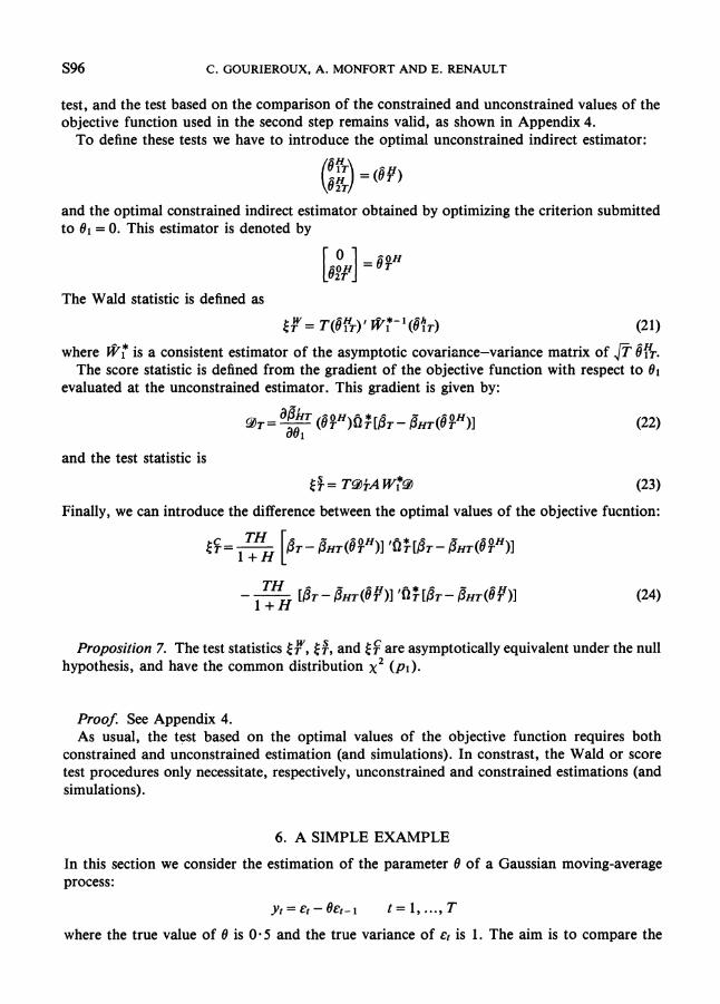
Figure 2. Estimated p.d.f. of the indirect estimator based on QP) ( ) and of the ML estimator (- --1
properties of the exact maximum likelihood estimator of 8, based on the Kalman filter algorithm, with those of several indirect estimators of 8 based on criteria of the form:
where r takes various values. For each experiment, the number of observations is T = 250 and the number of replications
is 200. In these experiments we only use one simulated path (H=1). Moreover, since the
C. GOURIEROUX, A. MONFORT AND E. RENAULT
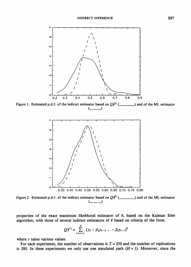
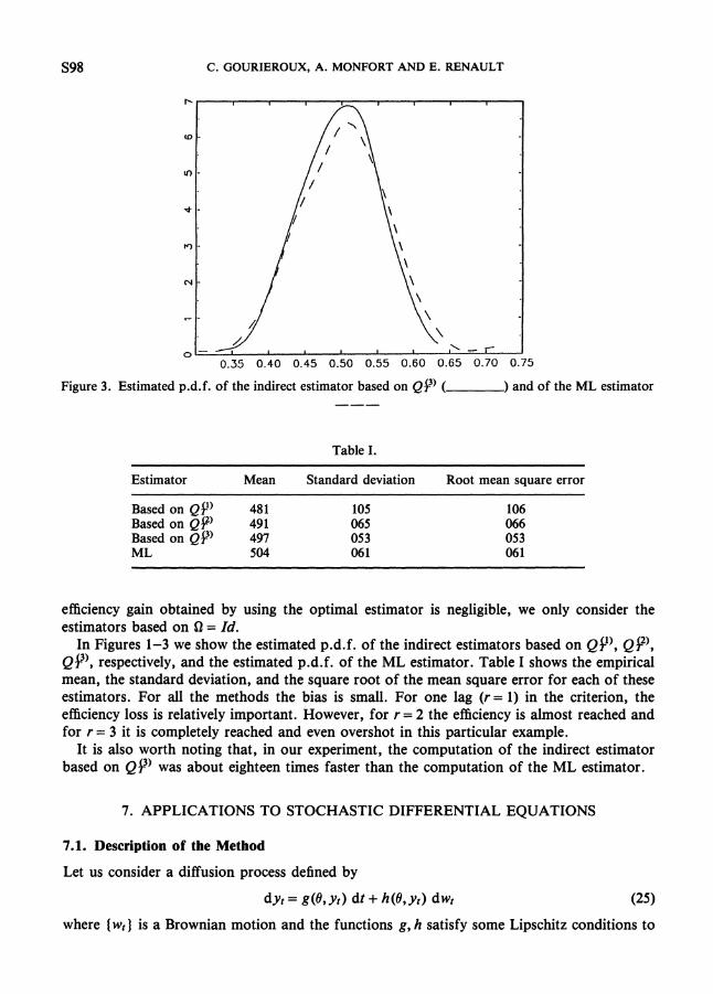
Figure 3. Estimated p.d.f. of the indirect estimator based on QP) ( ) and of the ML estimator
Table I.
Estimator Mean Standard deviation Root mean square error
Based on QY) 481 105 106 Based on QP) 491 065 066 Based on QP) 497 053 053 ML 504 061 06 1
efficiency gain obtained by using the optimal estimator is negligible, we only consider the estimators based on a= Id.
In Figures 1-3 we show the estimated p.d.f. of the indirect estimators based on Qjl), QY), QY) , respectively, and the estimated p.d.f. of the ML estimator. Table I shows the empirical mean, the standard deviation, and the square root of the mean square error for each of these estimators. For all the methods the bias is small. For one lag (r = 1) in the criterion, the efficiency loss is relatively important. However, for r = 2 the efficiency is almost reached and for r = 3 it is completely reached and even overshot in this particular example.
It is also worth noting that, in our experiment, the computation of the indirect estimator based on QY) was about eighteen times faster than the computation of the ML estimator.
7. APPLICATIONS TO STOCHASTIC DIFFERENTIAL EQUATIONS
7.1. Description of the Method
Let us consider a diffusion process defined by
where ( w t ) is a Brownian motion and the functions g, h satisfy some Lipschitz conditions to
INDIRECT INFERENCE s99
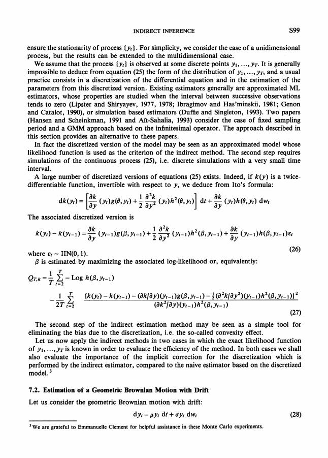
ensure the stationarity of process (y t ) . For simplicity, we consider the case of a unidimensional process, but the results can be extended to the multidimensional case.
We assume that the process (yt) is observed at some discrete points yl, ...,y ~ .It is generally impossible to deduce from equation (25) the form of the distribution of yl, ...,y ~ ,and a usual practice consists in a discretization of the differential equation and in the estimation of the parameters from this discretized version. Existing estimators generally are approximated ML estimators, whose properties are studied when the interval between successive observations tends to zero (Lipster and Shiryayev, 1977, 1978; Ibragimov and Has'minskii, 1981; Genon and Catalot, 1990), or simulation based estimators (Duffie and Singleton, 1993). Two papers (Hansen and Scheinkman, 1991 and Kit-Sahalia, 1993) consider the case of fixed sampling period and a GMM approach based on the infinitesimal operator. The approach described in this section provides an alternative to these papers.
In fact the discretized version of the model may be seen as an approximated model whose likelihood function is used as the criterion of the indirect method. The second step requires simulations of the continuous process (25), i.e. discrete simulations with a very small time interval.
A large number of discretized versions of equations (25) exists. Indeed, if k(y) is a twice- differentiable function, invertible with respect to y, we deduce from Ito's formula:
The associated discretized version is
where et - IIN(0,l). (26)
p is estimated by maximizing the associated log-likelihood or, equivalently:
The second step of the indirect estimation method may be seen as a simple tool for eliminating the bias due to the discretization, i.e. the so-called convexity effect.
Let us now apply the indirect methods in two cases in which the exact likelihood function of yl, ...,y~ is known in order to evaluate the efficiency of the method. In both cases we shall also evaluate the importance of the implicit correction for the discretization which is performed by the indirect estimator, compared to the naive estimator based on the discretized model.
7.2. Estimation of a Geometric Brownian Motion with Drift
Let us consider the geometric Brownian motion with drift:
'We are grateful to Emmanuelle Clement for helpful assistance in these Monte Carlo experiments.
sloe C. GOURIEROUX, A. MONFORT AND E. RENAULT
where (wt) is a Brownian motion of variance 1. We want to estimate 0 = (p, a) from discrete observations yl, ...,y ~ .
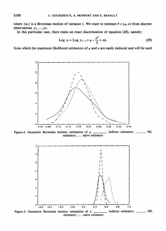
In this particular case, there exists an exact discretization of equation (28), namely:
a2Log yt= Log yt-1 +p- -+ act
2
from which the maximum likelihood estimators of p and a are easily deduced and will be used
Figure 4. Geometric Brownian motion: estimation of a. Indirect estimator; --- ML estimator: . . .. naive estimator
Figure 5. Geometric Brownian motion: estimation of a. Indirect estimator; --- ML estimator; .. . . naive estimator
INDIRECT INFERENCE s lo l
Table 11. Gometric Brownian motion
Estimator Mean Bias Standard deviation Root mean square error
ML p 0.201 0.001 0.040 a 0.503 0.003 0.030
Indirect p 0.201 0.001 0.057 a 0.499 -0.001 0.087
Naive p 0.220 0.020 0.049 a 0.624 0.124 0.061
0.040 0.045 0.050 0.055 0.060 0.065 0.070 0.075 0.000
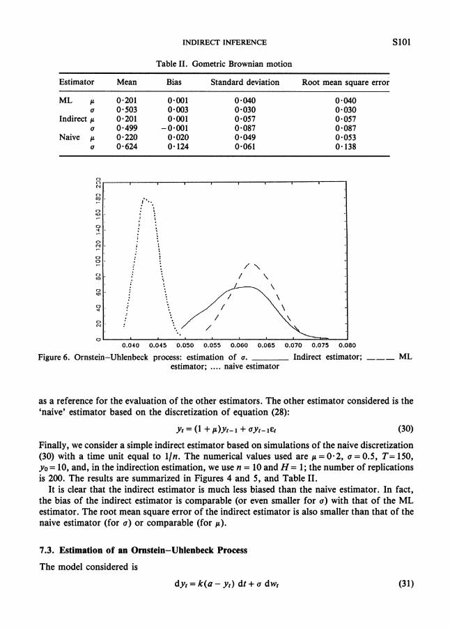
Figure 6. Ornstein-Uhlenbeck process: estimation of a. Indirect estimator; --- ML estimator; . . . . naive estimator
as a reference for the evaluation of the other estimators. The other estimator considered is the 'naive' estimator based on the discretization of equation (28):
Finally, we consider a simple indirect estimator based on simulations of the naive discretization (30) with a time unit equal to lln. The numerical values used are p = 0.2, a = 0.5, T = 150, yo = 10, and, in the indirection estimation, we use n = 10 and H= 1;the number of replications is 200. The results are summarized in Figures 4 and 5, and Table 11.
It is clear that the indirect estimator is much less biased than the naive estimator. In fact, the bias of the indirect estimator is comparable (or even smaller for a) with that of the ML estimator. The root mean square error of the indirect estimator is also smaller than that of the naive estimator (for a) or comparable (for p).
7.3. Estimation of an Ornstein-Uhlenbeck Process
The model considered is
s102 C . GOURIEROUX, A . MONFORT AND E. RENAULT
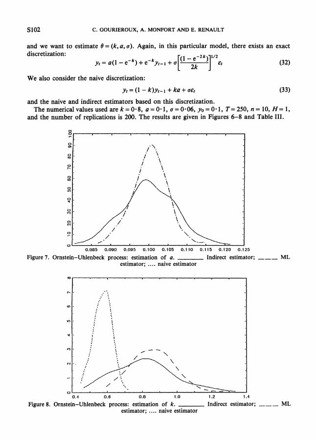
and we want to estimate 8 = (k, a, a). Again, in this particular model, there exists an exact discretization:
yt = a(1- e-k) + e-kyt-l + a (32)
We also consider the naive discretization:
yt = (1 - k)yt-1 + ka+ act
and the naive and indirect estimators based on this discretization. Thenumericalvaluesusedarek=0~8,a=0 .1 , a=0.06, y0=0-1 , T=250, n = 10, H = 1,
and the number of replications is 200. The results are given in Figures 6-8 and Table 111.
Figure 7. Ornstein-Uhlenbeck process: estimation of a. Indirect estimator; --- ML estimator; .... naive estimator
0.1 0.6 0.8 1 .O 1.2 1.4
Figure 8. Ornstein-Uhlenbeck process: estimation of k. Indirect estimator; estimator; .... naive estimator
INDIRECT INFERENCE S103
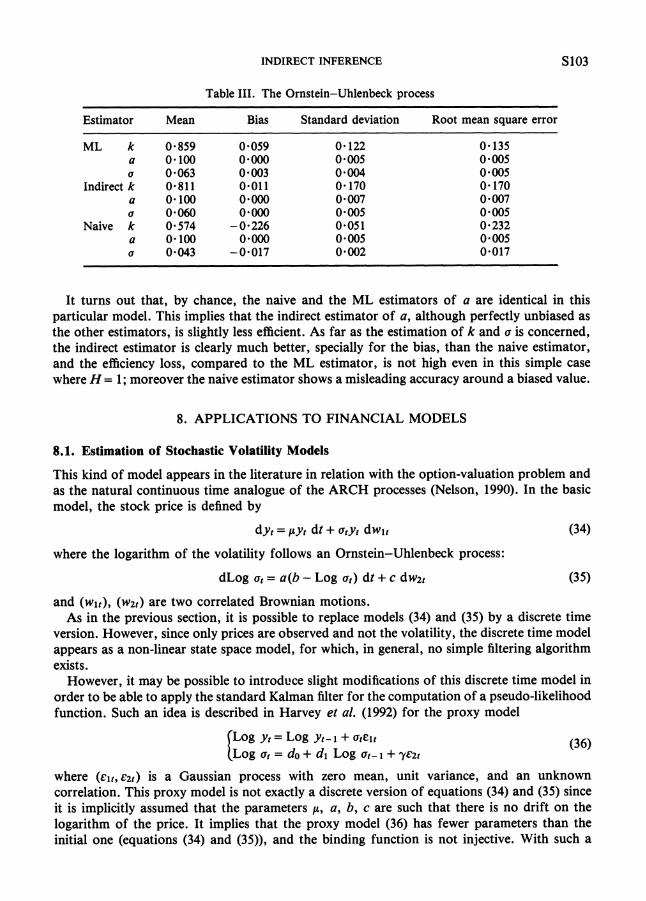
Table 111. The Ornstein-Uhlenbeck process
Estimator Mean Bias Standard deviation Root mean square error
ML k a u
Indirect k a Q
Naive k a Q
It turns out that, by chance, the naive and the ML estimators of a are identical in this particular model. This implies that the indirect estimator of a, although perfectly unbiased as the other estimators, is slightly less efficient. As far as the estimation of k and a is concerned, the indirect estimator is clearly much better, specially for the bias, than the naive estimator, and the efficiency loss, compared to the ML estimator, is not high even in this simple case where H= 1; moreover the naive estimator shows a misleading accuracy around a biased value.
8. APPLICATIONS TO FINANCIAL MODELS
8.1. Estimation of Stochastic Volatility Models
This kind of model appears in the literature in relation with the option-valuation problem and as the natural continuous time analogue of the ARCH processes (Nelson, 1990). In the basic model, the stock price is defined by
where the logarithm of the volatility follows an Ornstein-Uhlenbeck process:
dLog at = a(b - Log at) dt + c dwZt (35)
and (wit), (wzt) are two correlated Brownian motions. As in the previous section, it is possible to replace models (34) and (35) by a discrete time
version. However, since only prices are observed and not the volatility, the discrete time model appears as a non-linear state space model, for which, in general, no simple filtering algorithm exists.
However, it may be possible to introdnce slight modifications of this discrete time model in order to be able to apply the standard Kalman filter for the computation of a pseudo-likelihood function. Such an idea is described in Harvey et al. (1992) for the proxy model
Log yt = Log yt- 1 + ate1t Log at = do + dl Log at-1 + yezt
where (elt,ezt) is a Gaussian process with zero mean, unit variance, and an unknown correlation. This proxy model is not exactly a discrete version of equations (34) and (35) since it is implicitly assumed that the parameters p, a, b, c are such that there is no drift on the logarithm of the price. It implies that the proxy model (36) has fewer parameters than the initial one (equations (34) and (35)), and the binding function is not injective. With such a
S104 C.GOURIEROUX,A.MONFORT AND E. RENAULT
proxy model it is not possible to identify all the parameters by the indirect estimation approach. Nevertheless, if the proxy model is modified into
ILog yt = X + Log yt- 1 + Ut<
Log at = do + dl Log at- 1 + y ~ z t
and even if the Kalman filter does not apply to the above equaiton, we could use it inside a two-step procedure, as soon as (at) is stationary. Indeed, a consistent estimator of X is
and the Kalman filter may be applied to the variable Log(Log yt -Log yt- 1 -IT)' instead of Log(Log Yt/(Yt-1))2 in order to estimate the other auxiliary parameters do, dl, y.
Therefore it is possible to look for values of the parameters p, a, b, c, for which these two- step estimators of the auxiliary parameters determined from the observations and from the simulations, respectively, are close together. Of course, the general results on the asymptotic variance-covariance matrix are not valid for this two-step estimation procedure of the auxiliary parameter, but they can be extended to this case.
8.2. Factor ARCH Models
Multivariate ARCH models naturally contain a large number of parameters, and it is necessary to introduce constraints to make this number smaller. A usual approach, compatible with the needs of financial theory, leads to the introduction of unobserved factors, which drive the whole dynamics of the system (Diebold and Nerlove, 1989; Engle et al., 1989; King et al., 1990; GouriCroux et al., 1991). Let us consider, for instance, a one-factor model of the Diebold-Nerlove type:
yt = X f t + f t (38)
where (y t ) is the observable n-dimensional process, (f t) is a Gaussian white noise with an unknown variance-covariance matrix Q, (5)is a unidimensional unobserved factor independent of (a) ,and X gives the n sensitivity parameters of the components of yt to the common factor ft. We assume that the factor follows an ARCH(1) representation:
ft/fa -N[O, cro + crlf (with the identifying restriction a o + a1= 1) (39)
The p.d.f. of yl, fl, ...,YT,f~conditional to fo is: T
1 1 X- exp --
J 1( 2 ~ ) " ~ Z 2 cro + crlf ;-1
The likelihood function associated with the observable variables is
and has the form of an integral whose dimension is equal to the number of observations.
INDIRECT INFERENCE
Use of the extended Kalman jlter The model defined by equations (38) and (39) can be put in a state-space form:
f t = (ao+ a1f : - I ) ' / ~ ~ ~(transition equation)
yt = Aft + ~t (measurement equation)
with vt - IIN (0, l), independent of (el). These equations are non-linear with respect to the state ft. However, the extended Kalman filter can be used and, in this case, this simply amounts to replacing f ?- 1 in the transition equation by the square of the filtered value obtained at time t - 1. If this extended filter is used to compute an approximate likelihood function, the estimators obtained are inconsistent, but this estimator can also be considered as the first-step estimator of the indirect estimation method, which leads to a consistent estimator.
State discretization Another approach for approximating the exact log-likelihood function consists of
approximating directly the transition equation. For this purpose it is interesting to replace the initial factor by a discretized factor (see GouriCroux, 1992, Chapter 6). Let us consider a partition of the range of f t into K given classes (ak, ak+l), k = 0, ...,K - 1, with a0 = - a , ak = + a and let us define the discretized factor:
where bk, k = 0, ...,K - 1, are given real numbers, such as the centres of the classes, except for the extreme ones. Then we get:
P[X = bk/X-I = b/l = PCft-1E (ak, ak+l)/ft-1 E (a/, &+I))
= PUtE (ak,ak+i)/ft-I= br)
The initial factor ARCH model can be replaced by the proxy model:
where (et) , (f;] are independent, (et) - IIN(0, Q),and ( X ) is a qualitative Markov process with transition probabilities P ~ ~ ( c Y o , a1).
In this auxiliary model a recursive evaluation of the likelihood function is available (see Hamilton, 1989). Moreover, using Kitagawa's (1987) smoothing formula, the EM algorithm provides explicit expressions both at the E and at the M stage for the ML estimation of the unrestricted parameters. Therefore these parameters can be chosen as the auxiliary parameters and the expression of Pklabove can provide relevant starting values for the estimators of these parameters based on simulations.
9. APPLICATION TO MICROECONOMETRICS
In this section we describe a potential application to discrete-choice models. When the independence of irrelevant alternatives (IIA) hypothesis is not satisfied and a probit formulation is used, the log-likelihood function contains integrals whose dimension is equal to the number of alternatives minus one (McFadden, 1976; Hausman and Wise, 1978). When
S106 C. GOURIEROUX, A. MONFORT AND E. RENAULT
this dimension is small the integrals may be approximated by polynomial expansions: when it is reasonably large, they may be approximated by the Monte Carlo approach using, for instance, the simulated maximum likelihood method. The indirect estimation approach may also be used in the previous context for any dimension of the integrals. In this subsection we describe a logit approximation of the c.d.f. of a multivariate normal distribution. This approximation should be useful in various contexts and, in particular, for job-search models (see GouriCroux et al., 1992), or for the treatment of the serial correlation in limited dependent variables models (Robinson, 1982; Gourieroux et al., 1984).
Let Z be a Gaussian random vector, with zero mean and a variance-covariance matrix Id + R, where matrix R has a zero diagonal. We are interested in an approximation of the c.d.f.:
1 -00 -, [det(Zd+ R)] 'I2
expi-4z1(Zd+ R)-'21 dz ( 2 ~ ) ~ "
To obtain such an approximation, we use the expansion of the probability around R = 0. A first-order expansion gives:
where p and @ are the p.d.f. and the c.d.f. of the standard normal, and pkr the correlation between Zk and 21.
This approximation may be replaced by another, since:
Finally, we know that the logit distribution is close to the normal distribution N[O, (n2/3)]. Therefore if F(z) = l / ( l + exp(-2)) is the c.d.f. of the logistic distribution, we have approximately:
The above two expansions have two advantages. They avoid the computation of the initial integral and they have a product form, which makes simpler the expression of the log-probability:
Approximation (43) seems better than (42) since it also defines a c.d.f. of a multivariate distribution (see e.g. Thelot, 1981, for K = 2). It is not the case in (42). Moreover, it is easily seen that the marginal distribution associated with approximation (43) are logistic distributions ~((n/B)zk) . In Gourieroux et al. (1992) these results are used for job-search models.
A difficulty must be stressed in this kind of discrete-choice application. The simulated paths
INDIRECT INFERENCE S107
YTH(~)are not continuous with respect to 8 and, therefore, the classical asymptotic theory cannot be used. However, following Pakes and Pollard (1989), there is a way of building a generalized asymptotic theory.
10. APPLICATION TO MACROECONOMETRICS
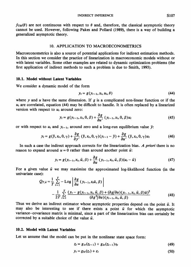
Macroeconometrics is also a source of potential applications for indirect estimation methods. In this section we consider the practice of linearization in macroeconomic models without or with latent variables. Some other examples are related to dynamic optimization problems (the first application of indirect methods to such a problem is due to Smith, 1993).
10.1. Model without Latent Variables
We consider a dynamic model of the form
where y and u have the same dimension. If g is a complicated non-linear function or if the ut are correlated, equation (44) may be difficult to handle. It is often replaced by a linearized version with respect to ut around zero:
or with respect to ut and yt-1, around zero and a long-run equilibrium value J:
In such a case the indirect approach corrects for the linearization bias. A priori there is no reason to expand around u = 0 rather than around another point ti:
yt = g(yt-1,xt, ti, PI +-ag (yt-1,xt, ti, P)(ut - ti) (47)au
For a given value ti we may maximize the approximated log-likelihood function (in the univariate case):
Q T , ~=-1 C =
- LogT t = l
1 (yt - x,, ti, P) + ( a g / a u ) ( ~ ~ - ~ , x ~ ,g ( ~ , - ~ , ti, --2T t = l
C ( a g 2 1 a ~ ) ( ~ t - l , ~ t ,ti, 0 )
Thus we derive an indirect estimator whose asymptotic properties depend on the point ti. It may also be interesting to see if there exists a point ti for which the asymptotic variance-covariance matrix is minimal, since a part of the linearization bias can certainly be corrected by a suitable choice of the value ti.
10.2. Model with Latent Variables
Let us assume that the model can be put in the nonlinear state space form:
Zt = glt(zt-1) + g2t(zt-l)?t
S108 C . GOURIEROUX, A. MONFORT AND E. RENAULT
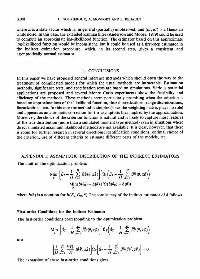
where zt is a state vector which is, in general (partially) unobserved, and (e : ,7:) is a Gaussian white noise. In this case, the extended Kalman filter (Anderson and Moore, 1979) could he used to compute an approximate log-likelihood function. The estimator based on this approximate log-likelihood function would be inconsistent, but it could be used as a first-step estimator in the indirect estimation procedure, which, in its second step, gives a consistent and asymptotically normal estimator.
11. CONCLUSIONS
In this paper we have proposed general inference methods which should open the way to the treatment of complicated models for which the usual methods are intractable. Estimation methods, significance tests, and specification tests are based on simulations. Various potential applications are proposed and several Monte Carlo experiments show the feasibility and efficiency of the methods. These methods seem particularly promising when the criterion is based on approximations of the likelihood function, time discretizations, range discretizations, linearizations, etc. In this case the method is simpler (since the weighting matrix plays no role) and appears as an automatic correction for the asymptotic bias implied by the approximation. Moreover, the choice of the criterion function is natural and is likely to capture most features of the true distribution (more than a simulated moment type method) even in situations where direct simulated maximum likelihood methods are not available. It is clear, however, that there is room for further research in several directions: identification conditions, optimal choice of the criterion, use of different criteria to estimate different parts of the models, etc.
APPENDIX 1: ASYMPTOTIC DISTRIBUTION OF THE INDIRECT ESTIMATORS
The limit of the optimization problem:
Min [b(I30) - b(I3)I 'Q(b(80) - b(I3)) e
where b(13) is a notation for ~ ( F o , GO,B).The consistency of the indirect estimator of 6 follows.
First-order Conditions for the Indirect Estimator
The first-order conditions corresponding to the optimization problem
are H l HC ag:r (BB, zo") h T P̂ T -- C p:(BQ, zo") =0[h,.I dB ] [ Id h = l 1
The expansion of these first-order conditions gives
INDIRECT INFERENCE
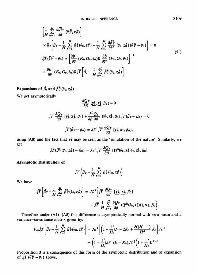
Expansions of Bt and $$(OO, z t )
We get asymptotically
aTx:, BT) =0(y:,ap --
using (A8) and the fact that y4 may be seen as the 'simulation of the nature'. Similarly, we
Asymptotic Distribution of
We have
Therefore under (A1)-(A8) this difference is asymptotically normal with zero mean and a variance-covariance matrix given by:
Proposition 3 is a consequence of this form of the asymptotic distribution and of expansion of fl(8; - 60) above.
silo C. GOURIEROUX, A. MONFORT AND E. RENAULT
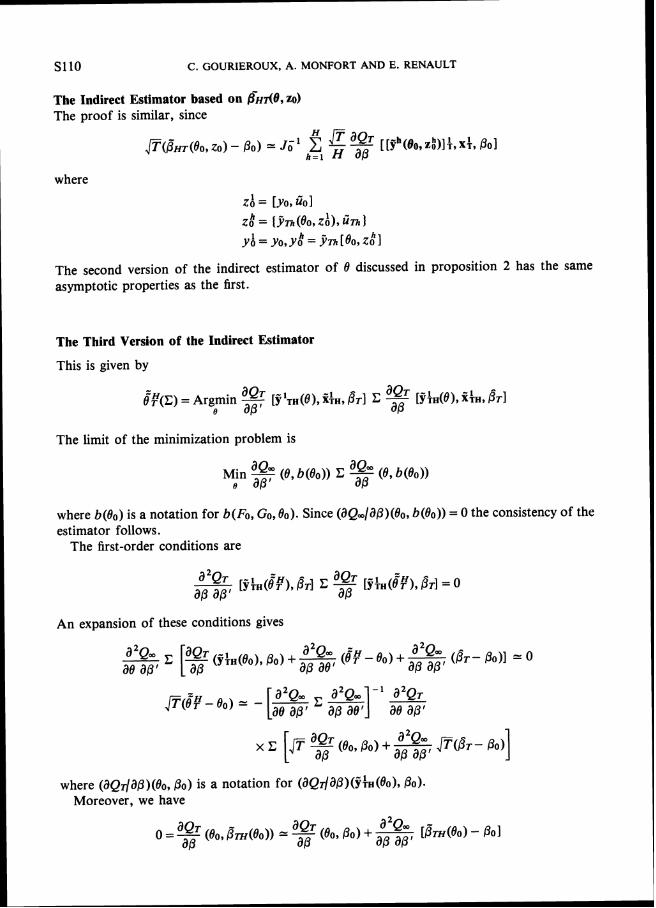
The Indirect Estimator based on h A 0 , ZO)
The proof is similar, since
where
zb = [yo,fiol oh = {jjm(eo,zb), I y b = y o , y o h = j ~ [ e o , ~ 6 ~
The second version of the indirect estimator of 8 discussed in proposition 2 has the same asymptotic properties as the first.
The Third Version of the Indirect Estimator
This is given by
BF(E) = [ ~ f t H ( d ) ,S ~ H , aQr
[ J + H ( B ) , i :~,Argmin Qy OTI E - OTI e a0 a0
The limit of the minimization problem is
Min 7aQw (8, b(8o)) E $$(8, b(8o)) e a0
where b(80)is a notation for b(Fo, GO, 80). Since (aQm/ap)(8o,b(80))= 0 the consistency of the estimator follows.
The first-order conditions are
An expansion of these conditions gives
where ( a Q ~ / a p ) ( 8 ~ , Po).po) is a notation for ( a ~ ~ / a p ) ( j : ~ ( e ~ ) , Moreover, we have
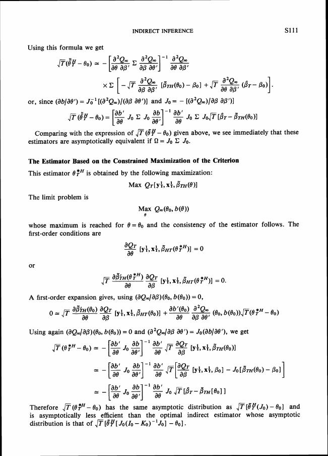
INDIRECT INFERENCE
Using this formula we get
a 2 ~ m X C [-P- [ B T H ( ~ o )- O O I + JT w (bT- o,)].
or, since (ab/ael)= J , '[(a2Qm)/(aOa0 ')I and JO= - [(a2Qm)/a0aO')l
Comparing with the expression of JT (8F- 80) given above, we see immediately that these estimators are asymptotically equivalent if i-2 = JOC Jo.
The Estimator Based on the Constrained Maximization o f the Criterion
This estimator 8:H is obtained by the following maximization:
Max QT[Y:, x i , D T H ( ~ ) ] The limit problem is
Max Qm(80, b(8)) 0
whose maximum is reached for 8 = 8, and the consistency of the estimator follows. The first-order conditions are
9ae [y:, x i , P H ~ ( B : ~ ) I= 0
A first-order expansion gives, using (aQm/aO)(80, b(eo)) =0,
Using again (aQ,/ap)(80, b(8o)) = 0 and (a2Qm/a0 8 ' ) = Jo(ab/ael),we get
Therefore P ( B ; ~ -has the same asymptotic distribution as @ [ ~ ? ( J o )- 801 and8,) is asymptotically less efficient than the optimal indirect estimator whose asymptotic distribution is that of JT [8F[ Jo(Io-KO)-'JO]- 901 .
--
C. GOURIEROUX, A. MONFORT AND E. RENAULT
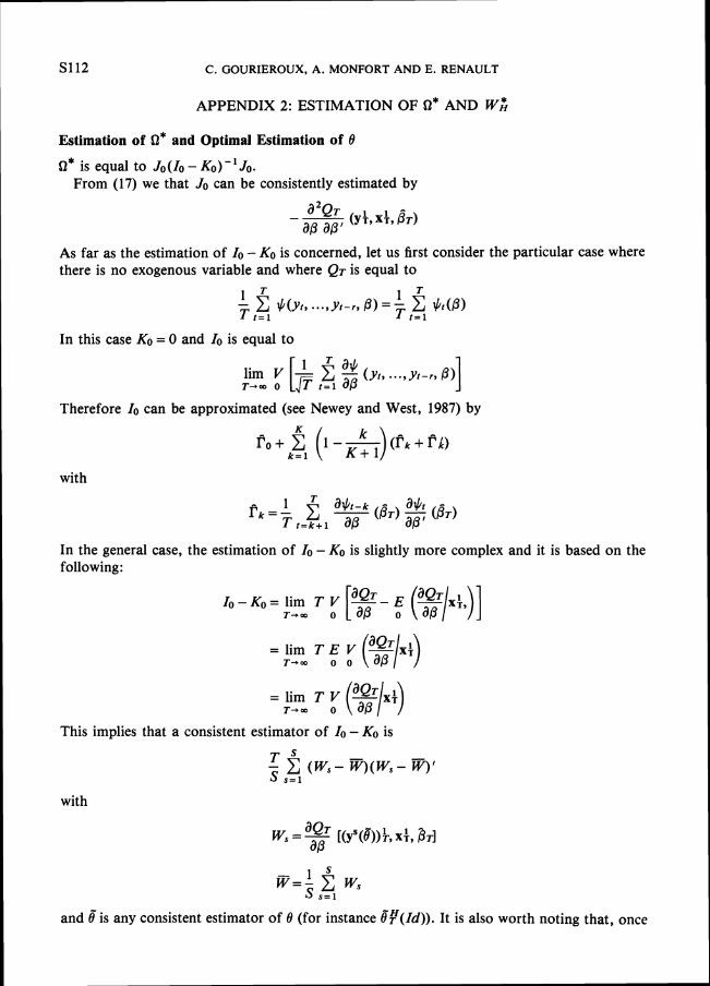
APPENDIX 2:ESTIMATION OF Q* AND W$
Estimation of Q* and Optimal Estimation of 8
Q* is equal to Jo(10 -KO)- 'Jo. From (17) we that JOcan be consistently estimated by
(yt, x i , BT) a0
As far as the estimation of lo-KO is concerned, let us first consider the particular case where there is no exogenous variable and where QT is equal to
In this case KO = 0 and 10is equal to
Therefore locan be approximated (see Newey and West, 1987) by
with
In the general case, the estimation of 10-KO is slightly more complex and it is based on the following:
10-KO= lim T V T-rw 0
This implies that a consistent estimator of 10-KO is
with
~ Q Tws=- [(yV<e')h x i , BTIa0
and 8 is any consistent estimator of 9 (for instance gF(1d)). It is also worth noting that, once
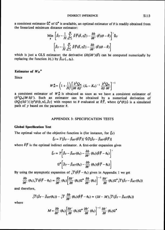
INDIRECT INFERENCE S113
a consistent estimator 0: of n* is available, an optimal estimator of 8 is readily obtained from the linearized minimum distance estimator:
which is just a GLS estimator; the derivative ( ab /ae1 ) (8 )can be computed numerically by replacing the function b ( . ) by ST(., 20).
Estimator of WH*
Since
a consistent estimator of W; is obtained as soon as we have a consistent estimator of ( a 2 ~ , / a 9 80 ' ) . by ( a Q ~ / a p ' ) g?,evaluated at 6' with respect to TI[(y"(e)hxi ,
Such an estimator can be obtained a numerical derivation of where ( yS (8 ) )kis a simulated
path of y based on the parameter 0 .
APPENDIX 3: SPECIFICATION TESTS
Global Specification Test
The optimal value of the objective function is (for instance, for &) {T = - [$T - ?)IT[P^T BHT(8?)1 ' 0 : P H T ( ~
where is the optimal indirect estimator. A first-order expansion gives
a b P ^ T - ~ H T ( o o ) - - - ; (eO)(I??-eo)ae 'I
a bn*[P T - B H T ( B ~ ) - , ( eo ) (BB-eo ) I By using the asymptotic expansion of p ( 8 ? - 90) given in Appendix 1 we get
and therefore,
~ ( B T -B H T ( ~ o ) )- f l ab (Bo)(BB- 00 )= ( I d- - BHT(eo))~ ) f l ( @ ~
where
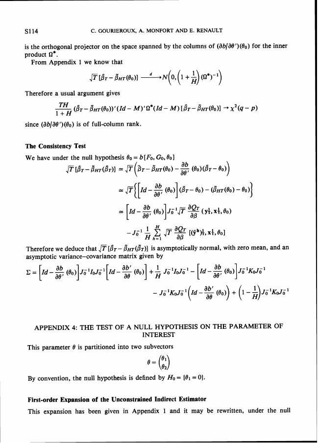
S114 C. GOURIEROUX, A. MONFORT AND E. RENAULT
is the orthogonal projector on the space spanned by the columns of (ab/aBf)(80)for the inner product Q*.
From Appendix 1 we know that
Therefore a usual argument gives
TH ( B T - B H T ( B O ) ) ( I ~ -M ) ' Q * ( I ~ -M ) [ P T - ~ H T ( ~ o ) ]* ~ ' ( 4 - P )l + H
since (ab/a8') (00)is of full-column rank.
The Consistency Test
We have under the null hypothesis 80= b [Fo, GO, 801
d [ B T - ~ H T ( ~ T ) ]= @ B T - ~ H T ( B O )-ab
( ~ o ) ( B r -$0)
Therefore we deduce that [ B T - &T(&)] is asymptotically normal, with zero mean, and an asymptotic variance-covariance matrix given by
APPENDIX 4: THE TEST OF A NULL HYPOTHESIS ON THE PARAMETER OF INTEREST
This parameter 8 is partitioned into two subvectors
By convention, the null hypothesis is defined by Ho = (81=01.
First-order Expansion of the Unconstrained Indirect Estimator
This expansion has been given in Appendix 1 and it may be rewritten, under the null
INDIRECT INFERENCE
hypothesis:
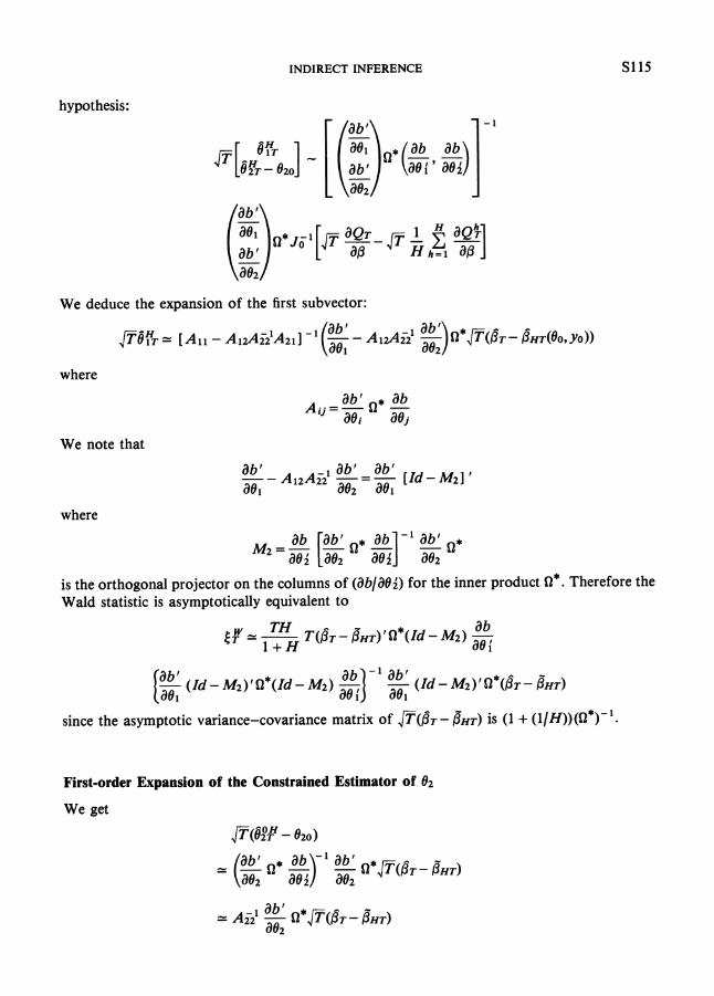
We deduce the expansion of the first subvector:
where
We note that
ab' 1 ab' ab'-- A12AT2-=- [Id-M2] ' ae ae2 ael where
is the orthogonal projector on the columns of (ab/aBi)for the inner product a* . Therefore the Wald statistic is asymptotically equivalent to
ab' (Id- M ~ ) ~ Q * ( I ~ - M ~ ) (Id- BHT)M ~ ) ' o * ( ~ T -
since the asymptotic variance-covariance matrix of ~ ( O T -BHT) is ( 1 + ( l / ~ ) ) ( n * ) - ' .
First-order Expansion of the Constrained Estimator of 02
We get
JT(820TH - 020)
S116 C. GOURIEROUX, A. MONFORT AND E. RENAULT
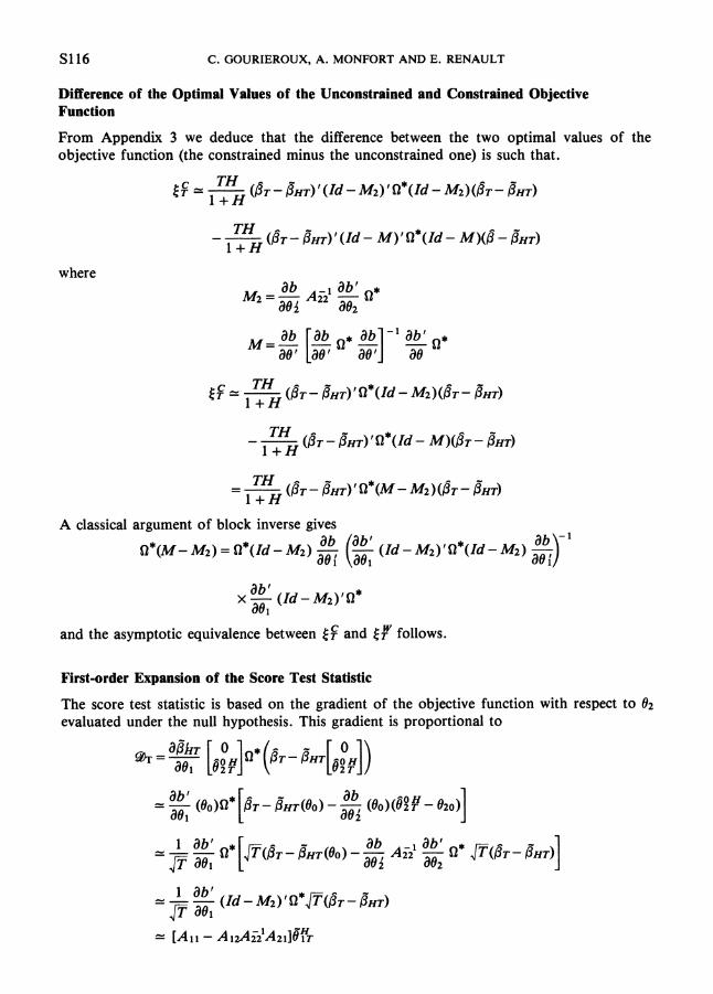
Difference of the Optimal Values of the Unconstrained and Constrained Objective Function
From Appendix 3 we deduce that the difference between the two optimal values of the objective function (the constrained minus the unconstrained one) is such that.
where
A classical argument of block inverse gives ab ab'
R*(M-M2) = Q*(ld-~ 2 )rn (z( ld -M2)'Q*(ld-~ 2 )
and the asymptotic equivalence between [$ and tr follows.
First-order Expansion of the Score Test Statistic
The score test statistic is based on the gradient of the objective function with respect to 02
evaluated under the null hypothesis. This gradient is proportional to
INDIRECT INFERENCE S117
There is asymptotically a one-to-one linear relationship betweenand 9 and i%f~ and this shows that the score test is asymptotically equivalent to the Wald test.
Asymptotic variance-covariance matrix of the unconstrained estimator &$and of the score
We get
and therefore we deduce
va,(JTgT)= 1 + - (All - A I ~ A T ~ A Z ~ )( 3 REFERENCES
Kit-Sahalia, Y. (1993), 'Nonparametric pricing of interest rate derivative securities', MIT. Anderson, B. D. 0. and J. B. Moore (1979), Optimal Filtering, Prentice-Hall, Englewood Cliffs, NJ. Diebold, F. and M. Nerlove (1989), 'The dynamic of exchange rate volatility: a multivariate latent factor
ARCH model', Journal of Applied Econometrics, 4 , 1-22. Duffie, D. and K. Singleton (1993), 'Simulated moments estimation of Markov models of asset prices'. Engle, R., V. Ng and M. Rothschild (1989)' 'Asset pricing with a factor ARCH covariance structure:
empirical estimates for treasury bills' UCSD DP, 89-31. Gallant, R. and G. Tauchen (1992), 'Which moments to match ?' Mimeo. Gallant, R. and H. White (1988), Estimation and Inference for Nonlinear Dynamic Models, Blackwell,
New York. Genon-Catalot, V. (1990)' 'Maximum contrast estimation for diffusion processes from discrete
observations', Statistics, 21, 99-116. GouriCroux, C. (1992), Modkles ARCH: Applications Financikres et Montftaires, Economica, Paris. GouriCroux C. and A. Monfort (1993)' 'Simulation based inference: a survey with special reference to
panel data models', Journal of Econometrics. GouriCroux, C. and A. Monfort (1992), 'Testing, encompassing and simulating dynamic econometric
models, CREST-DCpartement de la Recherche INSEE, DP No. 9214. GouriCroux, C., A. Monfort and E. Renault (1991), 'Dynamic factor models', CREST-DCpartement de
la Recherche INSEE. GouriCroux C., A. Monfort and E. Renault (1992), 'Indirect inference', CREST-Departement de la
Recherche INSEE, DP No. 9215. GouriCroux, C., A. Monfort and A. Trognon (1983), 'Testing nested or non-nested hypotheses', Journal
of Econometrics, 21, 83-1 15. GouriCroux, C., A. Monfort and A. Trognon (1984), 'Estimation and test in probit models with serial
correlation', in Florens et al. (eds), Alternative Approaches to Time Series Analysis, Publich-Universits St Louis, Brussels.
Hamilton, J. (1989), 'A new approach to the economic analysis of nonstationary time series and the business cycle', Econometrica, 57, 357-384.
Hansen, L. P. and J. Scheinkman (1991), 'Back to the future: generating moment implications for continuous time Markov processes', University of Chicago.
Hausman, J. and D. Wise (1978), 'A conditional probit model for qualitative choice: discrete decisions, recognizing interdependence and heterogeneous preferences', Econometrica, 46, 403-426.
Harvey, A., E. Ruiz and N. Shephard (1992), 'Multivariate stochastic variance models', LSE DP No. 132.
Hendry, D. F., and J. F. Richard (1990), 'Recent developments in the theory of encompassing, in B. Tulkens and H. Tulkens (eds), Contributions to Operation Research and Econometrics, the Twentieth Anniversary of CORE, Cornet, MIT Press, Cambridge, MA, 393-400.
Ibragimov, I. A. and R. Z. Has'minskii (1981), Statistical Estimation, Asymptotic Theory, Springer-Verlag, Berlin.
S118 C. GOURIEROUX, A. MONFORT AND E. RENAULT
King, M., E. Sentana and S. Wadhwani (1990), 'A heteroscedastic model of assets returns and risk premia with time varying volatility: an aplication to sixteen world stock markets', Mimeo, LSE.
Kitagawa, G. (1987), 'Non Gaussian state space modeling of nonstationary time series', Journal of the American Statistical Association, 82, 1032- 1041.
Kooreman, P. and G. Ridder (1983), 'The effects of age and unemployment percentage on the duration of unemployment', European Economic Review, 20, 41-57.
Lipster R. S. and A. N. Shiryayev (1977), Statistics of Random Processes I , General Theory, Springer-Verlag, Berlin.
Lipster, R. S. and A. N. Shiryayev (1978), Statistics of Random Processes 11, Applications, Springer-Verlag, Berlin.
McFadden, D. (1976), 'Quanta1 choice analysis: a survey', Annals of Economic and Social Measurement, 5, 363-390.
McFadden, D. (1989), 'A method of simulated moments for estimation of discrete response models without numerical integration', Econometrica, 57, 995-1026.
Mizon, G. E. and J. F. Richard (1986), 'The encompassing principle and its application to testing non nested hypotheses', Econometrica, 54, 657-678.
Nelson, D. B. (1990), 'ARCH models as diffusion approximations', Journal of Econometrics, 45, 7-38. Newey, W. K. and K. D. West (1987), 'A simple positive definite heteroscedasticity and autocorrelation
consistent covariance matrix', Econometrica, 55, 703-708. Pakes, A. and D. Pollard (1989), 'Simulation and the asymptotics of optimization estimators',
Econometrica, 57, 1027- 1058. Pesaran, H. and B. Pesaran (1991), 'A simulation approach to the problem of computing Cox's statistic
for testing non nested models', DP University of California at Los Angeles. Robinson, P. (1982), 'On the asymptotic properties of estimators of models containing limited dependent
variables', Econometrica, 50, 27-41. Smith, A. (1993), 'Estimating nonlinear time series models using simulated vector autoregressions',
Journal of Applied Econometrics, this issue. Thelot, C. (1981), 'Note sur la loi logistique et l'imitation', Annales de I'INSEE, 42, 111-125. Wooldridge, J. M. (1990), 'An encompassing approach to conditional mean tests with applications to
testing non nested hypotheses', Journal of Econometrics, 45, 331-350.
You have printed the following article:
Indirect InferenceC. Gourieroux; A. Monfort; E. RenaultJournal of Applied Econometrics, Vol. 8, Supplement: Special Issue on Econometric InferenceUsing Simulation Techniques. (Dec., 1993), pp. S85-S118.Stable URL:
http://links.jstor.org/sici?sici=0883-7252%28199312%298%3CS85%3AII%3E2.0.CO%3B2-7
This article references the following linked citations. If you are trying to access articles from anoff-campus location, you may be required to first logon via your library web site to access JSTOR. Pleasevisit your library's website or contact a librarian to learn about options for remote access to JSTOR.
References
The Dynamics of Exchange Rate Volatility: A Multivariate Latent Factor Arch ModelFrancis X. Diebold; Marc NerloveJournal of Applied Econometrics, Vol. 4, No. 1. (Jan. - Mar., 1989), pp. 1-21.Stable URL:
http://links.jstor.org/sici?sici=0883-7252%28198901%2F03%294%3A1%3C1%3ATDOERV%3E2.0.CO%3B2-T
A New Approach to the Economic Analysis of Nonstationary Time Series and the BusinessCycleJames D. HamiltonEconometrica, Vol. 57, No. 2. (Mar., 1989), pp. 357-384.Stable URL:
http://links.jstor.org/sici?sici=0012-9682%28198903%2957%3A2%3C357%3AANATTE%3E2.0.CO%3B2-2
A Conditional Probit Model for Qualitative Choice: Discrete Decisions RecognizingInterdependence and Heterogeneous PreferencesJerry A. Hausman; David A. WiseEconometrica, Vol. 46, No. 2. (Mar., 1978), pp. 403-426.Stable URL:
http://links.jstor.org/sici?sici=0012-9682%28197803%2946%3A2%3C403%3AACPMFQ%3E2.0.CO%3B2-8
http://www.jstor.org
LINKED CITATIONS- Page 1 of 3 -

Non-Gaussian State-Space Modeling of Nonstationary Time SeriesGenshiro KitagawaJournal of the American Statistical Association, Vol. 82, No. 400. (Dec., 1987), pp. 1032-1041.Stable URL:
http://links.jstor.org/sici?sici=0162-1459%28198712%2982%3A400%3C1032%3ANSMONT%3E2.0.CO%3B2-6
A Method of Simulated Moments for Estimation of Discrete Response Models WithoutNumerical IntegrationDaniel McFaddenEconometrica, Vol. 57, No. 5. (Sep., 1989), pp. 995-1026.Stable URL:
http://links.jstor.org/sici?sici=0012-9682%28198909%2957%3A5%3C995%3AAMOSMF%3E2.0.CO%3B2-Z
The Encompassing Principle and its Application to Testing Non-Nested HypothesesGrayham E. Mizon; Jean-Francois RichardEconometrica, Vol. 54, No. 3. (May, 1986), pp. 657-678.Stable URL:
http://links.jstor.org/sici?sici=0012-9682%28198605%2954%3A3%3C657%3ATEPAIA%3E2.0.CO%3B2-3
A Simple, Positive Semi-Definite, Heteroskedasticity and Autocorrelation ConsistentCovariance MatrixWhitney K. Newey; Kenneth D. WestEconometrica, Vol. 55, No. 3. (May, 1987), pp. 703-708.Stable URL:
http://links.jstor.org/sici?sici=0012-9682%28198705%2955%3A3%3C703%3AASPSHA%3E2.0.CO%3B2-F
Simulation and the Asymptotics of Optimization EstimatorsAriel Pakes; David PollardEconometrica, Vol. 57, No. 5. (Sep., 1989), pp. 1027-1057.Stable URL:
http://links.jstor.org/sici?sici=0012-9682%28198909%2957%3A5%3C1027%3ASATAOO%3E2.0.CO%3B2-R
On the Asymptotic Properties of Estimators of Models Containing Limited DependentVariablesPeter M. RobinsonEconometrica, Vol. 50, No. 1. (Jan., 1982), pp. 27-41.Stable URL:
http://links.jstor.org/sici?sici=0012-9682%28198201%2950%3A1%3C27%3AOTAPOE%3E2.0.CO%3B2-T
http://www.jstor.org
LINKED CITATIONS- Page 2 of 3 -
Estimating Nonlinear Time-Series Models Using Simulated Vector AutoregressionsA. A. Smith, JrJournal of Applied Econometrics, Vol. 8, Supplement: Special Issue on Econometric InferenceUsing Simulation Techniques. (Dec., 1993), pp. S63-S84.Stable URL:
http://links.jstor.org/sici?sici=0883-7252%28199312%298%3CS63%3AENTMUS%3E2.0.CO%3B2-H
http://www.jstor.org
LINKED CITATIONS- Page 3 of 3 -