1

Indirect estimation of signal-dependent noise withnon-adaptive heterogeneous samples

Lucio Azzari* and Alessandro FoiDepartment of Signal Processing, Tampere University of Technology

P.O. Box 553, FIN-33101 Tampere, Finland

Abstract—We consider the estimation of signal-dependentnoise from a single image. Unlike conventional algorithmsthat build a scatterplot of local mean-variance pairs fromeither small or adaptively selected homogeneous data samples,our proposed approach relies on arbitrarily large patches ofheterogeneous data extracted at random from the image. Wedemonstrate the feasibility of our approach through an extensivetheoretical analysis based on mixture of Gaussian distributions.A prototype algorithm is also developed in order to validate theapproach on simulated data as well as on real camera raw images.

Index Terms—Noise estimation, signal-dependent noise, Pois-son noise.

I. INTRODUCTION

The popularity of signal-dependent noise models, in whichthe variance of the noise affecting the signal depends onthe mean of the signal, is based on the fact that they wellapproximate noise affecting data of several kinds of acquisitiondevices, e.g., raw data from a CCD camera. Figure 1 illustrateshow the signal-dependent noise differently affects bright anddark regions of an image, and shows a curve that describesthe typical mean-variance relation of imaging sensors. Con-ventional methods [1], [6]–[13] estimate points of such mean-variance curve isolating and separately processing segments orpatches of the signal with common mean and noise variance,so that on each segment or patch simple sample estimators ofmean and variance can be applied. In this way, a scatterplot inthe mean-variance plane is produced. Then, a curve is fittedto the scatterplot, yielding an estimate of the relation for thewhole range of the signal.

In this paper we show that, contrary to common belief, theestimation can be accurate even if each scatterplot point is esti-mated from a heterogeneous sample (e.g., a patch whose pixelscan have very different mean values). We justify this resultthrough a mathematical modeling based on mixtures of normaldistributions. Thus, unlike conventional signal-dependent noiseestimation techniques that preprocess the image in order towork with homogeneous samples, our approach applies robustestimators to arbitrarily large patches of heterogeneous dataextracted at random from the image.

Our analysis is focused on the camera noise models such asthe affine-variance model depicted in Figure 1. For the sake of

Contact email: firstname.lastname@tut.fi.♥ This work was supported by the Academy of Finland (project no. 252547).Copyright (c) 2013 IEEE. Personal use of this material is permitted. However,permission to use this material for any other purposes must be obtained fromthe IEEE by sending a request to pubs-permissions@ieee.org.

(a) Noise-free image. (b) Noisy realization.

(c) Cross-section. (d) Mean7→variance relation.

Figure 1. Detail of the "Peppers" image corrupted by signal-dependent noisewith affine variance (2), with parameters a = 0.01 and b = 0.002.

clarity and due to length limitation, we restrict the presentationto the 2-D image case; nevertheless, the introduced conceptsand the proposed approach apply universally to 1-D signals aswell as to multidimensional data.

The paper is organized as follows. In Section II we introducethe considered signal-dependent noise model and we describethe conventional approach for its estimation. Next, we presentour novel noise estimation technique and a prototype algorithmthat exploits it, discussing its difference w.r.t. conventionalmethods. In Section III we study the main factors contributingto estimation errors, through a theoretical analysis and a MonteCarlo simulation. In Section IV we show the effectiveness ofthe method in real applications by estimating noise affectingraw data from a CCD camera, and a comparison with a state-of-the-art algorithm. Finally, in Section V and Section VI weprovide discussions and conclusions.

II. METHOD

A. Problem statement

Let us consider a noisy observation z of a deterministicnoise-free signal y, corrupted by additive spatially uncorrelatednoise with signal-dependent variance:

z(x) = y(x) + σ(y(x))ξ(x), (1)

2

0 0.1 0.2 0.3 0.4 0.5 0.6 0.7 0.8 0.9 10

0.005

0.01

0.015

0.02

0.025

yi

σ2i

(yi,σ2i )

fitted lineground truth

Figure 2. Scatterplot of the mean-variance pairs (yi,σ2i ), fitted line σ(y) =

ay + b, and ground truth line σ(y) = ay + b from the "Peppers" image,corrupted by noise with parameters a = 0.01 and b = 0.0017. We use 1000blocks of size 16× 16, each yielding a point in the scatterplot.

where σ : R → R+ is a function giving the signal-dependentstandard deviation of the noise, x ∈ X⊂ Z2 is the pixelcoordinate, and ξ : X → R is a zero-mean independentrandom noise with standard deviation equal to 1. Our goalis to estimate the function σ.The expectation of z(x), denoted as E{z(x)}, is the noise-free signal y(x); at the same time, the variance var{z(x)}and the standard deviation std{z(x)} of z(x) are, respectively,σ2(y(x)) and σ(y(x)), because var{y(x)} = 0.As discussed in [2], the term ξ(x) can generally have adifferent probability distribution for each different coordinatex, i.e. ξ(x1) � ξ(x2) if x1 6= x2; in order to simplify themathematical model, we approximate ξ(x) as a normal distri-bution N (0, 1). In this way the noise can be considered het-eroskedastic Gaussian, with zero mean and signal-dependentvariance σ2(y(x)), i.e. σ(y(x))ξ(x) ∼ N

(0, σ2(y(x))

).

To provide practical experimental results of our method,we shall refer to the affine noise variance model [5], whichis one of the most suitable for modeling the noise in digitalimage sensors. According to this model, the noise variance isapproximated as

σ2(y(x)) = ay(x) + b, (2)

where ay (x) and b are, respectively, the variances of thesignal-dependent and signal-independent parts of the noise.The former part is due to a photon-counting process (Poissondistribution), while the latter is caused by a combinationof dark noise (Poisson distribution) and thermal-electronicnoise (normal distribution). Because of a central-limit theoremargument and because of the good approximation of thePoisson by a Gaussian, the normal approximation of ξ(x) isvalid. For (2), the problem of estimating σ2 can be reducedto the estimation of the two constants a and b.

B. Conventional approach

The conventional approach for the estimation of signal-dependent noise is to segment the image into regions wherepixels have constant intensity, and hence, because of (1),constant noise; then, the mean and noise variance are estimatedfor each region independently. In this way it is possible tocreate a scatterplot that relates the noise-free intensity valuesof y (abscissa) with the respective noise variances (ordinate),that, finally, is used to approximate the function σ(y) in (1)(or equivalently the function σ2(y)).There are different methods for partitioning the image, withdifferent complexity and accuracy. The partition can be made,e.g., by simply using pixels extracted from a sufficiently smallwindow from the noisy image [9], with the constraint that theintensity does not change much within the window [7], [8], orby segmenting the image into level sets (bins) with individualintensity values [1], [6], [10], [11], [13]. More sophisticatedtechniques, such as DCT-based estimators [12], have beenalso proposed. However, the backbone idea is still to exploithomogeneous samples for the actual noise estimation.The rationale of these techniques is that, being the segmentshomogeneous, also the noise variance is homogeneous, as canbe trivially concluded from (1). Hence, standard estimators ofthe sample mean and sample variance can be directly appliedto the segments, yielding unbiased estimates of the mean andnoise variance. In other words, the resulting scatterplot pointsare distributed about the noise variance curve σ2(y).

C. Main idea

In contrast with the common procedure based on relativelysmall homogenous segments, we show that the estimationof each scatterplot point can be performed processing largeheterogeneous samples. As we shall demonstrate, consideringa heterogeneous group of elements taken from z, the expecta-tions of the estimators of its mean and noise variance are stilla coordinate of a point that belongs to the function σ2(y).Consequently, it is not necessary to partition the image intosegments of constant intensity levels and noise variances, but itis possible to process together parts of the image corrupted bynoise with various variance values, without compromising theestimation. In particular, adaptive segmentation is no longerrequired in order to estimate signal-dependent noise, but itsonly advantage consists in limiting the positive bias due tooutliers that could occur when estimating the variance. In thisway we can avoid the segmentation step and, consequently,simplify the entire process.We define our approach indirect because the pair estimatedfrom one block does not represent directly a single relationmean-noise variance, like for the conventional methods, butit represents the mean and the variance of an heterogeneousgroup of elements, i.e. a mixture of distributions.An example of the scatterplot computed from the blocks takenat random positions from the whole noisy image in Figure 1(a)is shown in Figure 2 (black dots), with its estimation of σ2(y)and the ground truth.

3

(a) Windowing in z. (b) Windowing in zH .

Figure 3. Example of 16× 16 windows at random position in z and atcorresponding positions in zH .

D. Prototype algorithm

The simplest algorithm that can leverage the above idea canbe divided in three basic steps:(a) High-Pass Filtering: most of the energy of the noise-free

signal y is usually confined to the lower frequencies of z,thus, applying an high-pass filter to z permits to extract thezero mean noise from it [3]. We obtain the high-frequencypart of z, referred to as zH , by convolving z against a 2-Dhigh-pass function ψ (e.g., a wavelet):

zH = z ~ ψ, (3)

where ψ has zero mean, i.e.∑i ψ(i) = 0, and `2-norm

equal to one, i.e.∑i ψ

2 (i) = 1.

(b) Local Estimation: once the detail image zH is computed,we randomly choose N coordinates within the image z,like in Figure 3; then, from these locations, N squareblocks W z

i , i = 1, . . . , N , of size√n×√n are extracted

from z. Similarly, N blocks WHi , i = 1, . . . , N , of the

same size and from the same positions of W zi , are ex-

tracted from zH . We estimate the means yi from the blocksW zi , while from WH

i we estimate the corresponding noisevariances σ2

i . In this way, for each block W zi , we obtain

a pair (yi,σ2i ) which can be represented by a point in the

scatterplot. The pairs (yi,σ2i ) are, therefore, the estimates

of the blocks means and noise variances (yi,σ2i ).

Because the blocks are taken from random positionswithin the image, each block may contain pixels havingvarious expected intensity levels. Therefore, the distribu-tion of noise in a single block W z

i can be considered asa mixture of normal distributions with different variances.This marks a principal difference with the conventionalmethods that look for uniform blocks (or regions) for theestimation, and that model the noise within a single blockas realization of a single normal distribution with givenmean and variance.In the next section we investigate the effects of exploitingelements taken from a mixture instead of from a singlenormal distribution.

(c) Fitting: in order to estimate the parameters that describethe curve σ2 (y), we fit the pairs (yi,σ2

i ), i = 1, . . . , N ,using a least squares (LS) method, which is the simplest

fitting technique at our disposal.

III. ESTIMATION ERROR

A. Noise analysis

Let us model image blocks as composed by Ri regions(piecewise modeling), with Ri ≤ n, and let W y

i denote thenoise-free block corresponding to W z

i .We shall refer as ideal the case in which, in WH

i , the amountof energy due to y is negligible with respect to the noiseenergy. For example, this is the case when W y

i can be treatedas piecewise constant with edges having small excursions withrespect to the noise standard deviation, or, equivalently, whenthe high-pass filter perfectly extract the noise component fromz. In this case, the elements of W z

i and WHi are, respectively,

realization of two mixtures of Ri normal distributions withprobability density functions (p.d.f.’s):

fzi (x) =Ri∑k=1

λ(i)k pzk (x), pzk ∼ N

(mk, s

2k

), (4)

fHi (x) =Ri∑k=1

λ(i)k pHk (x), pHk ∼ N

(0, s2k

), (5)

where pzk and pHk are, respectively, the p.d.f.’s of the k-thnormal distributions of fzi and fHi , λ(i)k is the proportion ofthe elements of the k-th population respect to the total numberof elements n, mk is the mean of the k-th normal function infzi , i.e. the k-th intensity value in W y

i , and s2k is the varianceof both pzk and pHk . It is important to notice that the idealityof this case relies mainly on the fact that the variances of thek-th distributions are equal.Trivially we have

yi =

Ri∑k=1

λ(i)k mk. (6)

Exploiting the moments of a general mixture of normaldistributions1, and the fact that all the pHk have zero mean,we obtain

σ2i =

Ri∑k=1

λ(i)k s2k. (7)

Considering now the particular Poisson-Gaussian noise, itfollows that the elements of WH

i can be individually modeledas realizations of independent normal random variables withvariances defined by the affine transformation (2) of W y

i :

s2k = amk + b.

1The expectation m and the variance s2 of a mixture of G normaldistributions are

m =G∑

k=1

νkmk,

s2 =

G∑k=1

νk

[(mk −m)2 + s2k

],

where mk , s2k and νk are, respectively, the expectation, the variance and theproportion of the k-th normal distribution [4].

4

Consequently, noting that∑Ri

k=1 λ(i)k = 1,

σ2i =

Ri∑k=1

λ(i)k amk +

Ri∑k=1

λ(i)k b =

aRi∑k=1

λ(i)k mk + b = ayi + b.

(8)

This means that the point (yi,σ2i ) belongs to the line (2).

Therefore, if yi and σ2i are computed, respectively, with

unbiased estimators of the population mean and variance of amixture of normal distributions, the points (yi,σ2

i ) will yield acloud scattered about the line (2), and the only error occurringin the computation of the pair (yi,σ2

i ) is the one due to thevariances of the estimators.The above proof shows that, in ideal conditions, the presentedalgorithm ensures correct estimation even using blocks af-fected by different noise levels.

Let us now consider a more practical scenario where thepresence of the noise-free signal WH

i is is still appreciable,influenced by strong edges and texture in W y

i . In this case, thenoise distribution in WH

i can no longer be approximated asa mixture of zero-mean normal distributions. In practice, thismeans that WH

i does not contain only noise, and that, amongits detail coefficients, there could be elements that introducea bias in the estimation of σ2

i . Consequently, the estimationerror does not depend only on the variance of the estimator,but it is also influenced by the presence of edges in W y

i .To reduce the effect of these outliers, we use the median ofabsolute deviation (MAD) [15], [16] as robust estimator ofσ2i and, for coherence, the median (med) as estimator of the

mean:yi = med {W z

i } , (9)

σ2i =

[MAD

{WHi

}Φ−1

(34

) ]2. (10)

Here, MAD{WHi

}= med

{∣∣WHi −med

{WHi

}∣∣}, andΦ−1 denotes the inverse cumulative distribution function(c.d.f.) of the standard normal distribution, and the constantfactor 1

/Φ−1

(34

)= 1.4826 makes the estimator asymptoti-

cally unbiased in case of i.i.d. normal samples.When using MAD, it is important to consider that the relation(8) may fail, because of the potential discrepancy between themean and the median of distributions that are not i.i.d. normal.Nevertheless, the use of the MAD estimator on WH

i can bejustified because of the Gaussianization of the coefficientsresulting by a transformation of the type (3) [2]. We supportthis thesis providing, in the next section, an accurate study ofthe robust estimators errors in practical applications.

B. Error analysis

As described in the previous section, the estimation erroris composed by two parts: one due to the variance of theestimators (the only one in the ideal case), and one due to thepresence of outliers (e.g., edges). In this section we analyzequantitatively how these outliers affect the computation of thepairs (yi,σ2

i ).For this purpose we performed a Monte Carlo simulation

B% = 10 B% = 15 B% = 20

n = 162

n = 642

Figure 4. Examples of the patches W yi used in the Monte Carlo simulation,

with different block sizes n and percentages of boundaries B%.

where we compute the average estimation error on a pair(yi,σ2

i ) from a block containing a certain amount of edges:• for each task, a patch containing a random number of

regions and corrupted by affine signal-dependent noise iscreated;

• the patches are then grouped depending on the amountof edges within them;

• the mean-noise variance pairs are then estimated;• the estimation errors are computed for each block;• finally, the errors are averaged, separately, for each group.

In this way, we compute the average estimation error infunction of the amount of edges in the block.

We now describe more accurately the entire process.1) Patch generation and grouping: we generate patches

W yi containing a random number of regions; each region

of each patch is piecewise smooth with piecewise smoothboundaries (examples are shown in Figure 4). The minimumand maximum intensity values of each region are realization ofrandom variables uniformly distributed in [0, 1]. The patchesare then grouped depending on the percentage of edges B%

within them. Every patch is corrupted by the noise definedin (2), and filtered as described in (3)2. In this way we createW zi and WH

i , which are used for computing yi and σ2i ,

respectively. The noise parameters a and b are chosen, for eachpatch, as realization of random variables uniformly distributedrespectively in [0, 0.002] and [0, 0.0006], in order to operate onnoise ranges comparable to those considered in, e.g., [1], [2],which are representative of typical consumer camera sensors.

2) Error computation and normalization: for every patch,the estimation error ei is computed as the distance between thepoint (yi,σ2

i ) estimated with (9) and (10), and the ground-truthline ay+b, i.e. the distance between (yi,σ2

i ) and its orthogonalprojection (yi⊥ ,σ2

i⊥) on the line ay + b.

Intuitively, the estimation errors of the mean and varianceare function of the noise variance that we are estimating,i.e. larger noise variance implies larger estimation error.Consequently, estimation errors on patches having the sameamount of edges, but affected by different noise levels, canbe significantly different. We normalize the square estimationerror e2i by dividing it by the mean square error (MSE) e2(σ2

i⊥)

that we would have had if we were performing the estimation

2To eliminate the boundary artifacts in the computation of WHi , we create

a bigger patch (padding) in order to discard the boundaries once the filteringis performed.

5

on a flat patch containing only one region, and affected byconstant noise variance σ2

i⊥. In this way, the normalized error

becomes an index of the goodness of the estimation withrespect to the simplest possible case, i.e. a single flat region.Let us now show how the MSE e2(·) depends on the noisevariance σ2 of a generic flat patch W

z, denoting W

Hits

filtered version:

MSE{

med{W z}}

= var{

med{W z}}

=vz(σ2)

= π2n σ

2,(11)

MSE{

MAD{WH

}}= var

{MAD

{WH

}}=

vH(σ2)

= αn σ

4,(12)

e2(σ2)

= vz(σ2)

sin2 (θ) + vH(σ2)

cos2 (θ) , (13)

where vz(σ2) and vH(σ2) are, respectively, the variances ofthe median and MAD estimators applied to the patches W

z

and WH

, and α is a constant that depends on the function3 ψ

that we use to filter Wz

in order to obtain WH

. The MSEsof the estimators coincide with their variances because thepatches are flat and the estimation errors have zero mean, i.e.the samples are unbiased because there are no outliers.In (13), the terms sin2 (θ) and cos2 (θ) are used to compute theorthogonal components of (11) and (12) to the line ay+b, theonly components of the variances that mislead the estimation,with θ being the angle between the line ay + b and thehorizontal axes, i.e. θ = arctan(a).We can finally define the normalized square estimation errore2i as

e2i =e2i

e2(σ2i⊥

). (14)

3) Averaging and error trend: Figure 5 shows the rootmean square error (RMSE) and the root mean normalizedsquare error (RMNSE) resulting from respectively averagingthe estimation errors e2i and e2i over groups of patches havingthe same percentage of edges B%. We separately consider fourdifferent window sizes n.

The RMNSE curves in Figure 5(b) are approximately mono-tonically increasing with common minimum 1 at B% = 0,where patches are composed of a single region and haveno internal edges. Note that the patches W y

i are piecewisesmooth, and not perfectly flat as in the ideal case; neverthelessat B% = 0 the RMNSE is practically 1. This means that, whenB% = 0, the RMSE essentially coincides with the standarddeviation of the estimator and, when B% > 0, the estimationerrors are almost entirely due to the presence of edges.

IV. EXPERIMENTS ON CAMERA RAW IMAGES

To validate the proposed algorithm in a practical context,we apply it to raw images from a digital camera. The imagesare shown in the left and center columns of Figure 6 and weretaken using a Canon PowerShot S90 10-Megapixel camera. We

3In our experiments ψ is generated by separable convolution of one 1-DDaubechies wavelet kernel,

ψ = ψ1D ⊗ ψT1D,

where ψ1D= [−0.333, 0.807,−0.460,−0.135, 0.085, 0.035]. For this ψ,we empirically computed α = 9.9076.

2% 6% 10% 14% 18%0

1

2

3

4

5

6x 10

−4

B%

RM

SE

n = 82

n = 162

n = 322

n = 642

(a) Root mean square error (RMSE).

2% 6% 10% 14% 18%0

1

2

3

4

5

6

7

8

B%

RM

NSE

n = 82

n = 162

n = 322

n = 642

(b) Root mean normalized square error (RMNSE).

Figure 5. RMSE and RMNSE as function of the percentage of edges B%within each block, for block size n = 82, 162, 322, 642. The estimationshave been performed using the robust estimators in (9) and (10).

adjusted the exposure times in order to avoid clipping (e.g.,overexposure). The pictures were acquired with various ISOsand exposure times, so to have realizations of different noiselevels [14].

In the rightmost column of Figure 6, the lines estimatedby the proposed prototype algorithm (continuous lines) arecompared against those estimated by a state-of-the-art al-gorithm [1] (dashed lines), here used as reference method.This algorithm first preprocesses the image in order to detectand exclude edges and texture from the noise estimation; itthen partitions the remaining image into segments of constantintensity level; a scatterplot is thus obtained by applying arobust unbiased estimator of the variance on each segment,with each point of the scatterplot being modeled according toa bivariate normal distribution; the noise model parameters aand b are finally estimated through a maximum a posteriorifitting. For these experiments, our prototype algorithms uses

6

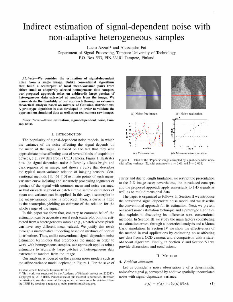
(a) Out-of-focus image. (b) Natural image. (c) Scatterplot and fitted lines.

(d) Out-of-focus image. (e) Natural image. (f) Scatterplot and fitted lines.

(g) Out-of-focus image. (h) Natural image. (i) Scatterplot and fitted lines.

Figure 6. Scatterplots and estimated functions for out-of-focus (red clouds and red continuous lines) and complex natural (blue clouds and blue continuouslines) images. The images have been taken with a Canon PowerShot S90, ISO 3200 (first row), ISO 2500 (second row), and ISO 200 (third row) usingexposure times respectively equal to 1/1000, 1/600, and 1/125. The estimation is performed using 2000 patches for each channel ([R,B;G1,G2]) of size64× 64. The dashed lines show the functions estimated by the ref. [1].

blocks of size 64× 64, and, in order to reduce the variabilityof the results on the particular random choice of the blockpositions, 2000 patches are extracted from each color channelof the images.

In Section III-A we discussed the theoretical behavior of ourmethod in the ideal conditions where the extracted patches arefree of edges (B% = 0 in Section III-B). In order to reproducethese assumptions, the raw images include 3 out-of-focus(OoF) pictures, shown in the leftmost column of Figure 6.The lines estimated by the two algorithms (red continuousand dashed lines) are always close to each other, confirmingthat, in the ideal case, the proposed algorithm gives resultscongruent to those of the reference algorithm.

The 3 pictures of a complex natural scene, shown in thecenter column of Figure 6 are used to investigate the practicalcase. The lines estimated with the proposed algorithm (blue

continuous lines) are again close to the reference ones (bluedashed lines), confirming that the proposed algorithm performssimilar to the reference algorithm also on complex images.

In Figure 6, the OoF and natural pictures that are on thesame row were acquired under the same operating conditions(ISO, exposure time, ambient temperature) and are hencecorrupted by noise with the same parameters [14]. Therefore,the blue solid and dashed lines in each subplot may beexpected to coincide with the respective red lines. Indeed,for large ISO (top and middle rows of Figure 6), the linesestimated from OoF and natural images are very close to eachother, because the large noise variance makes easier for thealgorithms to separate the noise from the noise-free signal.In case of small ISO (bottom row), instead, the estimationfrom the natural image diverges from the OoF ones, for bothproposed and reference algorithms, since the variance of the

7

0 0.1 0.2 0.3 0.40

1

2

3

4

5

6

7x 10

−5

(yi, σ2i ) (proposed)

(yi, σ2i ) (reference)

σ2pro(y)

σ2ref(y)

σ2(y)

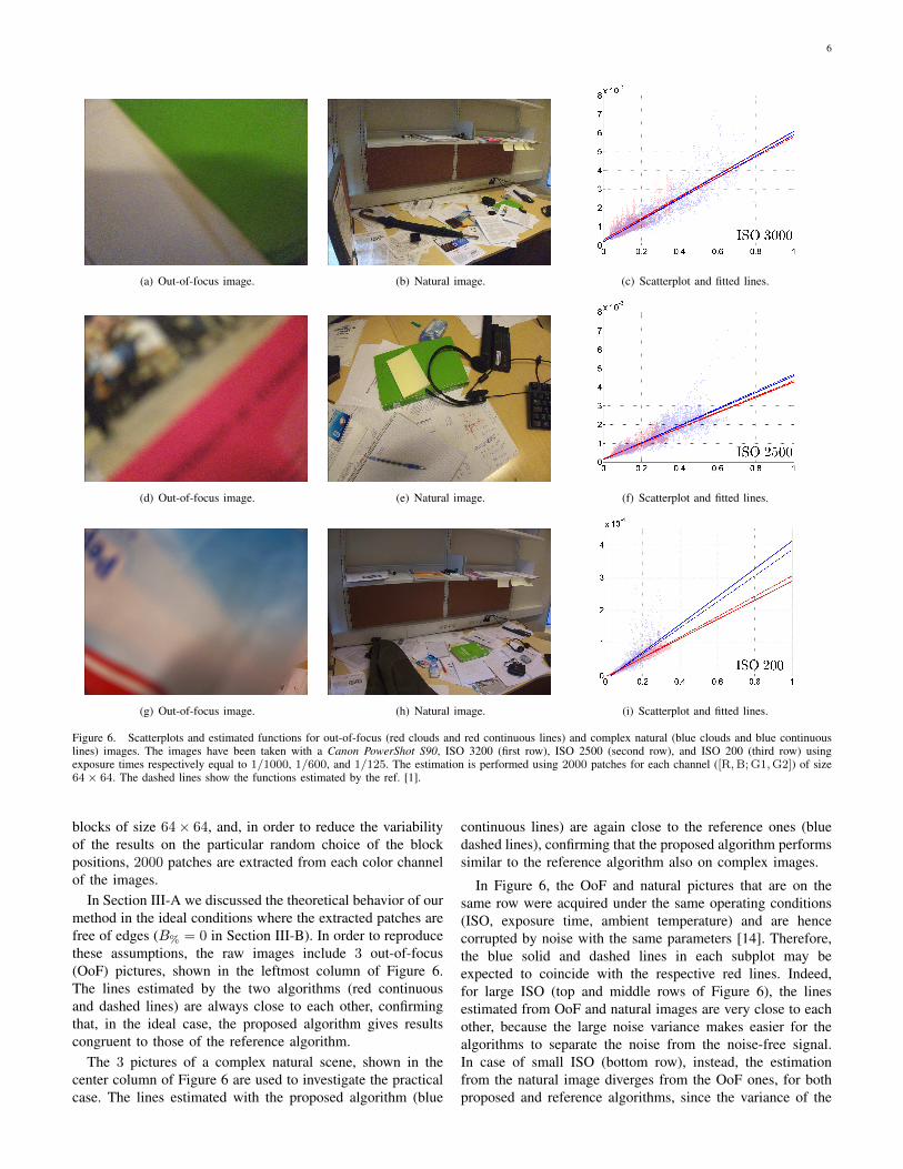
Figure 7. Example in which both proposed and reference algorithm failthe estimation due to the presence of several outliers. Top: image with largehighly textured areas from the NED dataset [20]. Bottom: scatterplot ofmean-variance pairs with corresponding noise line σ2

pro(y) estimated by theproposed prototype algorithm (red). The result is compared with the lineσ2ref(y) estimated using the reference algorithm (green) and the ground-truthσ2(y) (black). Due to the overwhelming presence of outliers in the scatterplot,both the proposed and the reference algorithm fail to correctly estimate thenoise line.

noise is small with respect to the signal. The degradation ofaccuracy of the proposed algorithm is comparable to that ofthe reference one.

In Figure 7 we report the result σ2pro(y) of the proposed

prototype algorithm applied to an image that contains largehighly textured areas. The image belongs to the NED dataset[20] of raw images with large areas of high-frequency texture,which makes noise estimation particularly challenging. Theimage has been captured with a Nikon D80 at ISO 125, andthe response of the sensor has been linearized by a calibratednonlinear correction function. In the same scatterplot we alsopresent the mean-variance pairs and the line σ2

ref(y) estimatedwith algorithm [1], and the ground-truth line σ2(y) too. Bothscatterplots reveal the presence of several outliers in the inten-sity range y ∈ [0, 0.1], mostly generated by textures present onthe mountains. These outliers cause the misestimation of thelines fitted by either the proposed and the reference algorithm4.This result confirms that textures and edges are the maincause of misestimation, since they affect similarly proposedand reference algorithm, and that the scatterplot points can beestimated using heterogeneous samples.

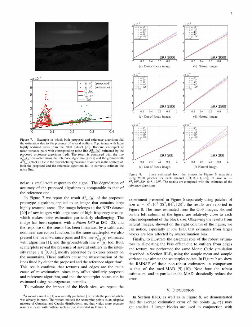
To evaluate the impact of the block size, we repeat the

4A robust variant of [1] was recently published [19] while the present articlewas already in press. The variant models the scatterplot points as an adaptivemixture of Gaussian and Cauchy distributions, and thus yields more accurateresults in cases with outliers such as that illustrated in Figure 7.

0 0.2 0.4 0.6 0.8 10

2

4

6

8x 10−3

ISO 3000

n = 82

n = 162

n = 322

n = 642

n = 1282

ref

(a) Out-of-focus image.

0 0.2 0.4 0.6 0.8 10

2

4

6

8x 10−3

ISO 3000

n = 82

n = 162

n = 322

n = 642

n = 1282

ref

(b) Natural image.

0 0.2 0.4 0.6 0.8 10

1

2

3

4

5x 10−3

ISO 2500

n = 82

n = 162

n = 322

n = 642

n = 1282

ref

(c) Out-of-focus image.

0 0.2 0.4 0.6 0.8 10

1

2

3

4

5x 10−3

ISO 2500

n = 82

n = 162

n = 322

n = 642

n = 1282

ref

(d) Natural image.

0 0.2 0.4 0.6 0.8 10

1

2

3

4

5x 10−4

ISO 200

n = 82

n = 162

n = 322

n = 642

n = 1282

ref

(e) Out-of-focus image.

0 0.2 0.4 0.6 0.8 10

1

2

3

4

5x 10−4

ISO 200

n = 82

n = 162

n = 322

n = 642

n = 1282

ref

(f) Natural image.

Figure 8. Lines estimated from the images in Figure 6 separatelyusing 2000 patches for each channel ([R,B;G1,G2]) of size n =82, 162, 322, 642, 1282. The results are compared with the estimates of thereference algorithm.

experiment presented in Figure 6 separately using patches ofsize n = 82, 162, 322, 642, 1282; the results are reported inFigure 8. The lines estimated from the OoF images, showedon the left column of the figure, are relatively close to eachother independent of the block size. Observing the results fromnatural images, showed on the right column of the figure, wecan notice, especially at low ISO, that estimates from largerblocks are less affected by overestimation bias.

Finally, to illustrate the essential role of the robust estima-tors in alleviating the bias effect due to outliers from edgesand texture, we performed the same Monte Carlo simulationdescribed in Section III-B, using the sample mean and samplevariance to estimate the scatterplot points. In Figure 9 we showthe RMNSE of these non-robust estimators in comparisonto that of the med-MAD (9)-(10). Note how the robustestimators, and in particular the MAD, drastically reduce theerror.

V. DISCUSSION

In Section III-B, as well as in Figure 8, we demonstratedthat the average estimation error of the points (yi,σ2

i ) mayget smaller if larger blocks are used in conjunction with

8

2% 6% 10% 14% 18%1

20

40

60

80

B%

RM

NSE

median-MADsample mean-sample variance

Figure 9. Root mean normalized square error (RMNSE) of the pairs median-MAD and sample mean-sample variance for blocks of size n = 322. Robustestimators lead to such a reduction of error also for the other block sizes.

robust estimators, in spite of the fact that the samples getmore heterogeneous. However, there is also an inevitabletrade-off in the choice of the block size: when using largepatches it is unlikely that the mean (or median) yi reachesthe extremes of the distribution of the image intensity valuesy. As a consequence, the scatterplot may cluster about thepoint (c, ac + b), c being the mean (or median) of y overthe whole image, and, thus, the accuracy of the estimated linemay be degraded. On the other hand, smaller patches allowthe scatterplot points to distribute on a wider interval, at theexpense of higher estimation variance for each point, and riskof larger bias on some of them. While the variance errorsmay cancel out through the curve fitting, the bias errors willeventually corrupt the final estimate unless a robust line fittingis utilized.

In Figure 9, the average error for robust and standardestimators are compared, demonstrating the complete failurecaused by non robust.

Our analysis and algorithm are developed and validatedon the specific affine-variance model (2), and may fail fora generic non-affine σ2(y). On the other hand, if σ2 is wellapproximated by a locally (i.e. separately on each block) affinefunction of y, we can still use the proposed algorithm, ensuringaccurate results. However, in many cases (e.g., in the case ofclipping) it can be difficult to verify the local affinity of σ2

without any strong assumptions on the image y.Let us discuss also about ways how to possibly improve

the estimation accuracy. In its prototype implementation, ouralgorithm is limited by the accuracy of the MAD estimator andthus cannot reach the accuracy of algorithms (e.g., [17]) thatadopt more sophisticated estimators for the estimation of thevariance. Likewise, the simplest LS fitting method is not robustto outliers in the scatterplot. Therefore, the use of a bettervariance estimator and a better (e.g., robust) fitting algorithm[19] could further improve the estimation, so to possibly dealwith highly textured images such as the example in Figure 7.

Adaptive procedures such as segmentation may be crucialfor alleviating the impact of high-frequency texture on thevariance estimation, but we especially emphasize that this is

not a peculiarity of signal-dependent noise models, and it ap-plies also to constant-variance (homoskedastic) noise models,including additive white Gaussian noise (AWGN). In fact, theadvanced methods [17] and [18] are developed for AWGNestimation. As shown in our theoretical and experimentalanalysis, the fact that the variance of the noise is not constant(heteroskedasticity), and depends instead on the signal, doesnot per se imply an additional need for adaptive segmentation.

Finally, let us note that the proposed model deals withthe estimation of signal-dependent noise that is spatiallyuncorrelated, i.e. noise with diagonal covariance matrix. It isnevertheless possible to extend the proposed approach alsoto the correlated-noise case. If the correlation model (i.e. theshape of the noise power spectral density (PSD)) is known,one can compute the noise energy in the high-pass image zH

from which the blocks WHi are extracted, and hence normalize

the output of the variance estimator based on the productof the PSD with the spectrum of ψ. This product can bepreconditioned by suitably downsampling the data prior toanalyzing the noise; downsampling may be also desirable, asa means to reduce the amount of data to be processed.

VI. CONCLUSIONS

As opposed to conventional methods that require homo-geneous samples for the estimation of mean-variance pairs,our approach to signal-dependent noise estimation utilizesarbitrarily large samples of possibly heterogeneous data. Theapproach is backed by a Gaussian-mixture modeling, whichshows that the individual mean-variance estimates computedfrom the heterogeneous samples are still representative of thetrue mean-variance curve. An elementary prototype algorithmbased on this modeling is presented for the estimation ofsignal-dependent noise from a single image. The algorithmextracts large heterogeneous samples from random locationsin the image. This corresponds to a fundamental differenceversus traditional algorithms, which often involve an adaptivesegmentation of the image into narrow homogeneous seg-ments, and it also results in a simplification of the estimationprocedure. This approach can be therefore suitable in allapplications where a simple noise estimation algorithm isrequired, and which has to operate on non-intelligent devices.Experiments on real data demonstrate the reliability of thealgorithm applied to natural images, showing that its resultsare comparable with those from a state-of-the-art method.

REFERENCES

[1] A. Foi, M. Trimeche, V. Katkovnik, and K. Egiazarian, PracticalPoissonian-Gaussian noise modeling and fitting for single image raw-data, IEEE Trans. Image Process., vol. 17, no. 10, pp. 1737-1754,October 2008.doi:10.1109/TIP.2008.2001399.

[2] A. Foi, Clipped noisy images: heteroskedastic modeling and practicaldenoising, Signal Processing, vol. 89, no. 12, pp. 2609-2629, Decem-ber 2009.doi:10.1016/j.sigpro.2009.04.035.

[3] D.L. Donoho and I.M. Johnstone, Ideal spatial adaptation via waveletshrinkage, Biometrika (1994) 81(3): 425-455.doi:10.1093/biomet/81.3.425.

[4] N. Johnson, S. Kotz, and N. Balakrishnan, Continuous UnivariateDistributions, vol. 1, Wiley & Sons, New York, Second edition, 1994,Section 13.10.

9

[5] G.K. Froehlich, J.F. Walkup, and R.B. Asher, Optimal estimation insignal-dependent noise, JOSA, Vol. 68, Issue 12, pp. 1665-1672, 1978.doi: 10.1364/JOSA.68.001665.

[6] C. Liu, W. T. Freeman, R. Szeliski and S. B. Kang, Noise Estimationfrom a Single Image, Proceedings of the 2006 IEEE Computer SocietyConference on Computer Vision and Pattern Recognition, CVPR ’06,vol. 1, pp. 901- 908, 17-22 June 2006.doi: 10.1109/CVPR.2006.207.

[7] A. Amer and E. Dubois, Fast and reliable structure-oriented videonoise estimation, IEEE Transactions on Circuits and Systems for VideoTechnology, vol. 15, no. 1, pp. 113-118, January 2005.doi: 10.1109/TCSVT.2004.837017(410) 1.

[8] S. Aja-Fernández, G. Vegas-Sánchez-Ferrero, M. Martín-Fernández andC. Alberola-López, Automatic noise estimation in images using localstatistics. Additive and multiplicative cases, Image and Vision Comput-ing, vol. 27, Issue 6, pp. 756-770, ISSN 0262-8856, 4 May 2009.doi: 10.1016/j.imavis.2008.08.002.

[9] J.S. Lee and K. Hoppel, Noise Modeling and Estimation of Remotely-Sensed Images, Geoscience and Remote Sensing Symposium, 1989.IGARSS’89. International 12th Canadian Symposium on Remote Sens-ing, vol.2, no., pp.1005-1008, 10-14 July 1989.doi: 10.1109/IGARSS.1989.579061.

[10] P. Gravel, G. Beaudoin and J.A. De Guise, A method for modeling noisein medical images, Medical Imaging, on IEEE Transactions, vol.23,no.10, pp.1221-1232, October 2004.doi: 10.1109/TMI.2004.832656.

[11] B. Aiazzi, L. Alparone, S. Baronti, M. Selva and L. Stefani, Unsu-pervised estimation of signal-dependent CCD camera noise, SpringerInternational Publishing AG, EURASIP Journal on Advances in SignalProcessing, No.1, pp. 1-11, 2012.doi: 10.1186/1687-6180-2012-231.

[12] M. Uss, B. Vozel, V. Lukin, S. Abramov, I. Baryshev, K. Chehdi, ImageInformative Maps for Estimating Noise Standard Deviation and TextureParameters, EURASIP Journal on Advances in Signal Processing, No.1, vol. 2011, p. 806516, 2011.doi: 10.1155/2011/806516.

[13] T. Buades, Y. Lou, J.M. Morel, Zhongwei Tang, A note on multi-image denoising, International Workshop on Local and Non-LocalApproximation in Image Processing, 2009. LNLA 2009, pp. 1-15, 2009.doi: 10.1109/LNLA.2009.5278408.

[14] P. Ojala, Dependence of the parameters of digital image noise modelon ISO number, temperature and shutter time, prepared for the 2008TUT/Nokia Mobile Imaging course.http://www.cs.tut.fi/∼foi/MobileImagingReport_PetteriOjala_Dec2008.pdf

[15] F. R. Hampel, The influence curve and its role in robust estimation,Journal of the American Statistical Association, vol. 69 (346), pp. 383-393, 1974.

[16] F. Mosteller and J.W. Tukey, Data Analysis and Regression: A SecondCourse in Statistics, Addison Wesley, 1997.

[17] A. Danielyan and A. Foi, Noise variance estimation in nonlocal trans-form domain, Proc. Int. Workshop on Local and Non-Local Approx. inImage Process., LNLA 2009, Tuusula, Finland, pp. 41-45, August 2009.doi:10.1109/LNLA.2009.5278404

[18] N.N. Ponomarenko, V.V. Lukin, M.S. Zriakhov, A. Kaarna and J.Astola, An automatic approach to lossy compression of AVIRIS images,Geoscience and Remote Sensing Symposium, 2007. IGARSS 2007.IEEE International. pp. 472-475, 2007.doi: 10.1109/IGARSS.2007.4422833.

[19] L. Azzari and A. Foi, Gaussian-Cauchy Mixture Modeling for RobustSignal-Dependent Noise Estimation, in Proc. IEEE ICASSP2014, pp.5394-5398, May 2014.

[20] Image database for benchmarking signal-dependent noise estimation al-gorithms: NED2012, Online: http://rsd.khai.edu/ned2012/ned2012.php.Accessed date: December 2013.