Embed Size (px)
Citation preview
HAL Id: tel-00746163https://tel.archives-ouvertes.fr/tel-00746163
Submitted on 27 Oct 2012
HAL is a multi-disciplinary open accessarchive for the deposit and dissemination of sci-entific research documents, whether they are pub-lished or not. The documents may come fromteaching and research institutions in France orabroad, or from public or private research centers.
L’archive ouverte pluridisciplinaire HAL, estdestinée au dépôt et à la diffusion de documentsscientifiques de niveau recherche, publiés ou non,émanant des établissements d’enseignement et derecherche français ou étrangers, des laboratoirespublics ou privés.
Indicators of Allophony and PhonemehoodLuc Boruta
To cite this version:Luc Boruta. Indicators of Allophony and Phonemehood. Linguistics. Université Paris-Diderot - ParisVII, 2012. English. <tel-00746163>
UNIVERSITÉ PARIS–DIDEROT (PARIS 7)ÉCOLE DOCTORALE INTERDISCIPLINAIRE EUROPÉENNE FRONTIÈRES DU VIVANT
DOCTORAT NOUVEAU RÉGIME— SCIENCES DU VIVANT
LUC BORUTA
INDICATORS ofALLOPHONY & PHONEMEHOOD
INDICATEURS D’ALLOPHONIE ET DE PHONÉMICITÉ
Thèse sous la direction deBenoît CRABBÉ & Emmanuel DUPOUX
Soutenue le 26 septembre 2012
JURYMme Martine ADDA-DECKER, rapporteuseMme Sharon PEPERKAMP, rapporteuseM. John NERBONNE, examinateurM. Benoît CRABBÉ, directeur de thèseM. Emmanuel DUPOUX, directeur de thèse

CONTENTS
Acknowledgements 5
Abstract 7
1 Introduction 111.1 Problem at hand . . . . . . . . . . . . . . . . . . . . . . . . . . . . . . . . . . . . . . 111.2 Motivation and contribution . . . . . . . . . . . . . . . . . . . . . . . . . . . . . . . 111.3 Structure of the dissertation . . . . . . . . . . . . . . . . . . . . . . . . . . . . . . . 12
2 Of Phones and Phonemes 132.1 The sounds of language . . . . . . . . . . . . . . . . . . . . . . . . . . . . . . . . . 13
2.1.1 Phones and phonemes . . . . . . . . . . . . . . . . . . . . . . . . . . . . . . 132.1.2 Allophony . . . . . . . . . . . . . . . . . . . . . . . . . . . . . . . . . . . . . 16
2.2 Early phonological acquisition: state of the art . . . . . . . . . . . . . . . . . . . . 172.2.1 Behavioral experiments . . . . . . . . . . . . . . . . . . . . . . . . . . . . . 182.2.2 Computational experiments . . . . . . . . . . . . . . . . . . . . . . . . . . . 20
3 Sources of Data 253.1 The Corpus of Spontaneous Japanese . . . . . . . . . . . . . . . . . . . . . . . . . 25
3.1.1 Data preprocessing . . . . . . . . . . . . . . . . . . . . . . . . . . . . . . . . 263.1.2 Data-driven phonemics . . . . . . . . . . . . . . . . . . . . . . . . . . . . . 273.1.3 The phonemic inventory of Japanese . . . . . . . . . . . . . . . . . . . . . . 31
3.2 Good allophones like yo momma used to cook . . . . . . . . . . . . . . . . . . . . 323.2.1 Old recipes for allophonic rules . . . . . . . . . . . . . . . . . . . . . . . . . 333.2.2 Allophonic rules redux . . . . . . . . . . . . . . . . . . . . . . . . . . . . . 35
3.3 Allophonic inventories . . . . . . . . . . . . . . . . . . . . . . . . . . . . . . . . . . 413.3.1 Data-driven phonotactics . . . . . . . . . . . . . . . . . . . . . . . . . . . . 423.3.2 O theory, where art thou? . . . . . . . . . . . . . . . . . . . . . . . . . . . . 45
4 Indicators of Allophony 514.1 Allophony: definitions and objectives . . . . . . . . . . . . . . . . . . . . . . . . . 51
4.1.1 Phones, phone pairs, and allophones . . . . . . . . . . . . . . . . . . . . . 514.1.2 Objectives: predicting allophony . . . . . . . . . . . . . . . . . . . . . . . . 52
4.2 Building indicators of allophony . . . . . . . . . . . . . . . . . . . . . . . . . . . . 544.2.1 Acoustic indicators . . . . . . . . . . . . . . . . . . . . . . . . . . . . . . . . 544.2.2 Temporal indicators . . . . . . . . . . . . . . . . . . . . . . . . . . . . . . . 564.2.3 Distributional indicators . . . . . . . . . . . . . . . . . . . . . . . . . . . . . 584.2.4 Lexical indicators . . . . . . . . . . . . . . . . . . . . . . . . . . . . . . . . . 61
4.3 Numerical recipes . . . . . . . . . . . . . . . . . . . . . . . . . . . . . . . . . . . . . 634.3.1 Turning similarities into dissimilarities . . . . . . . . . . . . . . . . . . . . 64
4 Contents
4.3.2 Standardizing indicators . . . . . . . . . . . . . . . . . . . . . . . . . . . . . 644.3.3 Addressing the frequency effect . . . . . . . . . . . . . . . . . . . . . . . . 65
4.4 Prognoses of allophony . . . . . . . . . . . . . . . . . . . . . . . . . . . . . . . . . . 684.4.1 Rank-sum test of class separation . . . . . . . . . . . . . . . . . . . . . . . . 684.4.2 Combining indicators of allophony . . . . . . . . . . . . . . . . . . . . . . . 754.4.3 Confusion plots: a look at indicators’ distributions . . . . . . . . . . . . . . 77
4.5 Predicting allophony: binary classification task . . . . . . . . . . . . . . . . . . . . 824.5.1 Binomial logistic regression . . . . . . . . . . . . . . . . . . . . . . . . . . . 834.5.2 Evaluation . . . . . . . . . . . . . . . . . . . . . . . . . . . . . . . . . . . . . 854.5.3 Results . . . . . . . . . . . . . . . . . . . . . . . . . . . . . . . . . . . . . . . 89
4.6 Overall assessment . . . . . . . . . . . . . . . . . . . . . . . . . . . . . . . . . . . . 95
5 Indicators of Phonemehood 975.1 Phonemehood: definitions and objectives . . . . . . . . . . . . . . . . . . . . . . . 97
5.1.1 Limitations of the pairwise framework . . . . . . . . . . . . . . . . . . . . 985.1.2 Objectives: predicting phonemehood . . . . . . . . . . . . . . . . . . . . . 99
5.2 Predicting phonemehood: (n+1)-ary classification task . . . . . . . . . . . . . . . 1015.2.1 Flat-response multinomial logistic regression . . . . . . . . . . . . . . . . . 1025.2.2 Nested-response multinomial logistic regression . . . . . . . . . . . . . . . 1035.2.3 Evaluation . . . . . . . . . . . . . . . . . . . . . . . . . . . . . . . . . . . . . 1045.2.4 Results . . . . . . . . . . . . . . . . . . . . . . . . . . . . . . . . . . . . . . . 106
5.3 Overall assessment . . . . . . . . . . . . . . . . . . . . . . . . . . . . . . . . . . . . 114
6 Phonemehood Redux 1156.1 Shifting the primitive data structure . . . . . . . . . . . . . . . . . . . . . . . . . . 115
6.1.1 Multidimensional scaling . . . . . . . . . . . . . . . . . . . . . . . . . . . . 1166.1.2 Visualizing phone configurations . . . . . . . . . . . . . . . . . . . . . . . . 121
6.2 Prognoses of phonemehood . . . . . . . . . . . . . . . . . . . . . . . . . . . . . . . 1256.3 Predicting phonemehood: n-ary classification task . . . . . . . . . . . . . . . . . . 127
6.3.1 Multinomial logistic regression . . . . . . . . . . . . . . . . . . . . . . . . . 1276.3.2 Evaluation . . . . . . . . . . . . . . . . . . . . . . . . . . . . . . . . . . . . . 1286.3.3 Results . . . . . . . . . . . . . . . . . . . . . . . . . . . . . . . . . . . . . . . 128
6.4 Predicting phonemehood: ?-ary clustering task . . . . . . . . . . . . . . . . . . . . 1326.4.1 Density-based clustering with DBSCAN . . . . . . . . . . . . . . . . . . . . 1336.4.2 Evaluation . . . . . . . . . . . . . . . . . . . . . . . . . . . . . . . . . . . . . 1356.4.3 Results . . . . . . . . . . . . . . . . . . . . . . . . . . . . . . . . . . . . . . . 137
6.5 Predicting phonemehood: n-ary clustering task . . . . . . . . . . . . . . . . . . . . 1416.5.1 Chances of phonemehood . . . . . . . . . . . . . . . . . . . . . . . . . . . . 1416.5.2 Complete-linkage hierarchical clustering . . . . . . . . . . . . . . . . . . . 1426.5.3 Evaluation . . . . . . . . . . . . . . . . . . . . . . . . . . . . . . . . . . . . . 1436.5.4 Results . . . . . . . . . . . . . . . . . . . . . . . . . . . . . . . . . . . . . . . 143
6.6 Overall assessment . . . . . . . . . . . . . . . . . . . . . . . . . . . . . . . . . . . . 150
7 Conclusion 1517.1 Indicators of allophony and phonemehood . . . . . . . . . . . . . . . . . . . . . . 1517.2 Future research . . . . . . . . . . . . . . . . . . . . . . . . . . . . . . . . . . . . . . 153
References 157

ACKNOWLEDGEMENTS
I had wonderful support and encouragement while preparing this dissertation. First and fore-most, Benoît Crabbé—my advisor and longtime maître à penser—provided invaluable feedback,expert insight, and inspirational discussion during the six years I spent working my way upthrough the computational linguistics program at Paris Diderot. His wise selection of textbooks,Belgian beers, and programming tips never proved wrong.
Emmanuel Dupoux—my other advisor—gave essential critical feedback throughout my grad-uate studies. He also provided me with a large quantity of excellent data on which to work.Sharon Peperkamp, Martine Adda-Decker, and John Nerbonne graciously agreed—and on
short notice—to carefully proofread my work with scientific rigour and a critical eye. I thankthem for their enthusiastic and constructive comments.François Taddei and Samuel Bottani welcomed me into a top-notch graduate school and an
even more exciting and accepting community of knowledge addicts. I learned a great deal intheir company, including new ways to learn. I owe them both a tremendous amount of gratitude.Charlotte Roze—my partner in misery—has been a constant source of support in and out of
the academic world. She knows that we can have it all, and everything will be alright.Finally, a big thank goes out to Benoît Healy who has supported me beyond measure, and
who spent hours considerately chasing the Frenglish in this dissertation. I know his brain hurts.So, come up to the lab, and see what’s on the slab...

ABSTRACT
Although we are only able to distinguish between a finite, small number of sound categories—i.e. a given language’s phonemes—no two sounds are actually identical in the messages wereceive. Given the pervasiveness of sound-altering processes across languages—and the fact thatevery language relies on its own set of phonemes—the question of the acquisition of allophonicrules by infants has received a considerable amount of attention in recent decades. How, forexample, do English-learning infants discover that the word forms [kæt] and [kat] refer to thesame animal species (i.e. cat), whereas [kæt] and [bæt] (i.e. cat ∼ bat) do not? What kind of cuesmay they rely on to learn that [sINkIN] and [TINkIN] (i.e. sinking ∼ thinking) can not refer to the sameaction? The work presented in this dissertation builds upon the line of computational studiesinitiated by Peperkamp et al. (2006), wherein research efforts have been concentrated on thedefinition of sound-to-sound dissimilarity measures indicating which sounds are realizations ofthe same phoneme. We show that solving Peperkamp et al.’s task does not yield a full answerto the problem of the discovery of phonemes, as formal and empirical limitations arise fromits pairwise formulation. We proceed to circumvent these limitations, reducing the task ofthe acquisition of phonemes to a partitioning-clustering problem and using multidimensionalscaling to allow for the use of individual phones as the elementary objects. The results ofvarious classification and clustering experiments consistently indicate that effective indicators ofallophony are not necessarily effective indicators of phonemehood. Altogether, the computationalresults we discuss suggest that allophony and phonemehood can only be discovered fromacoustic, temporal, distributional, or lexical indicators when—on average—phonemes do nothave many allophones in a quantized representation of the input.


In the beginning it was too far away for Shadow to focus on. Then itbecame a distant beam of hope, and he learned how to tell himself ‘thistoo shall pass’.~
—Neil Gaiman, in American Gods

CHAPTER 1INTRODUCTION
1.1 Problem at hand
Sounds are the backbone of daily linguistic communication. Not all natural languages havewritten forms; even if they do, speech remains the essential medium on which we rely todeliver information—mostly because it is always at one’s disposal, particularly when othercommunicationmedia are not. Furthermore, verbal communication often appears to be effortless,even to children with relatively little experience using their native language. We are hardlyconscious of the various linguistic processes at stake in the incessant two-way coding thattransforms our ideas into sounds, and vice versa.The elementary sound units that we use as the building blocks of our vocalized messages
are, however, subject to a considerable amount of variability. Although we are only able todistinguish between a finite, small number of sound categories—that linguists refer to as a givenlanguage’s phonemes—no two sounds are actually identical in the messages we receive. Soundsdo not only vary because everyone’s voice is unique and, to some extent, characterized by one’sgender, age, or mood, they also vary because each language’s grammar comprises a substantialnumber of so called allophonic rules that constrain the acoustic realization of given phonemes ingiven contexts. In English, for example, the first /t/ in tomato is—beyond one’s control—differentfrom the last: whereas the first, most likely transcribed as [th], is followed by a burst of air, thelast is a plain [t] sound. This discrepancy emblematizes a feature of the grammar of Englishwhereby the consonants /p/, /t/, and /k/ are followed by a burst of air—an aspiration—whenthey occur as the initial phoneme of a word or of a stressed syllable. Given the pervasiveness ofsuch sound-altering processes across languages—and the fact that every language relies on itsown set of phonemes—the question of the acquisition of allophonic rules by infants has receiveda considerable amount of attention in recent decades. How, for example, do English-learninginfants discover that the word forms [kæt] and [kat] refer to the same animal species (i.e. cat),whereas [kæt] and [bæt] (i.e. cat ∼ bat) do not ?
1.2 Motivation and contribution
Broadly speaking, research on early language acquisition falls into one of two categories: be-havioral experiments and computational experiments. The purpose of this dissertation is topresent work carried out for the computational modeling of the acquisition of allophonic rulesby infants, with a focus on the examination of the relative informativeness of different types ofcues on which infants may rely—viz. acoustic, temporal, distributional, and lexical cues.
The work presented in this dissertation builds upon the line of computational studies initiatedby Peperkamp et al. (2006), wherein research efforts have been concentrated on the definition ofsound-to-sound dissimilarity measures indicating which sounds are realizations of the same
12 Introduction
phoneme. The common hypothesis underlying this body of work is that infants are able tokeep track of—and rely on—such dissimilarity judgments in order to eventually cluster similarsounds into phonemic categories. Because no common framework had yet been proposed tosystematically define and evaluate such empirical measures, our focus throughout this studywas to introduce a flexible formal apparatus allowing for the specification, combination, andevaluation of what we refer to as indicators of allophony. In order to discover the phonemicinventory of a given language, the learning task introduced by Peperkamp et al. consists inpredicting—for every possible pair of sounds in a corpus, given various indicators of allophony—whether or not two sounds are realizations of the same phoneme. In this dissertation, weshow that solving this task does not yield a full answer to the problem of the discovery ofphonemes, as formal and empirical limitations arise from its pairwise formulation. We proceedto revise Peperkamp et al.’s framework and circumvent these limitations, reducing the task ofthe acquisition of phonemes to a partitioning-clustering problem.Let us emphasize immediately, however, that no experiment reported in this dissertation is
to be considered as a complete and plausible model of early language acquisition. The reasonfor this is twofold. First, there is no guarantee that the algorithms and data structures used inour simulations bear any resemblance to the cognitive processes and mental representationsavailable to or used by infants. Second, we focused on providing the first empirical boundson the learnability of allophony in Peperkamp et al.’s framework—relying, for instance, onsupervised learning techniques and non-trivial simplifying assumptions regarding the natureof phonological processes. Though motivated by psycholinguistic considerations, the presentstudy is thus to be considered a contribution to data-intensive experimental linguistics.
1.3 Structure of the dissertation
The body of this dissertation is divided into six main chapters, delimited according to thedifferent data representations and classification or clustering tasks we examined.In Chapter 2, we introduce the major concepts at play in the present study—viz. those of
phone, phoneme, and allophone. We also review in this chapter the state of the art in the fieldof computational modeling of early phonological acquisition. Chapter 3 is an introduction tothe corpus of Japanese speech we used throughout this study. Here, the focus is on discussingour preprocessing choices—especially regarding the definition of the phonemic inventory, themechanisms we used to control the limits of the phonetic similarity between the allophones of agiven phoneme, and how our data eventually relate to theoretical descriptions of the phonologyof Japanese. In Chapter 4, we report our preliminary experiments on the acquisition of allophony.We first define the core concepts of our contribution—viz. empirical measures of dissimilaritybetween phones referred to as indicators of allophony. Then, we evaluate these indicators inexperiments similar to the ones carried out by Peperkamp et al. (2006; and subsequent studies),and try to predict whether two phones are realizations of the same phoneme. Chapter 5 is dividedinto two main sections. In the first section, we discuss the limitations of Peperkamp et al.’spairwise framework, as well as our arguments in favor of a transition toward the fundamentalproposition of this study, i.e. not only predicting whether two phones are realizations of the samephoneme but, if so, of which phoneme they both are realizations. In the section that follows,we report various transitional experiments where, using the very same data as in Chapter 4, weattempt to classify phone pairs into phoneme-like categories. In Chapter 6, we start with a formaldescription of the techniques we used to obtain a novel, pair-free representation for the data athand that is more suitable to the prediction of phonemehood. We then go on to report variousclassification and clustering experiments aiming at partitioning a set of phones into a putativephonemic inventory. Finally, Chapter 7 contains a general conclusion in which we discuss thecontributions of the present study, as well as the limitations and possible improvements to ourcomputational model of the early acquisition of phonemes.
CHAPTER 2OF PHONES AND PHONEMES
When embarking on a study of sounds and sound systems, it is important to first define theobjects with which we will be dealing. As we are dealing with both tangible sound objectsand abstract sound categories, we need to define just what these objects are, as well as how weconceive the notion of sound category itself. Therefore, the aim of this chapter is to introduce themajor concepts at play in the present study (namely those of phone, phoneme, and allophone),and to review the state of the art in the area of computational modeling of early phonologicalacquisition.
2.1 The sounds of language
The subfields of linguistics can ideally be organized as a hierarchy wherein each level uses theunits of the lower level to make up its own, ranging from the tangible yet meaningless (at leastwhen considered in isolation) acoustic bits and pieces studied in phonetics, to the meaningful yetintangible abstract constructs studied in semantics and discourse. In this global hierarchy wherediscourses are made of utterances, utterances are made of words, etc., phonology and phoneticscan be thought of as the two (tightly related) subfields concerned with the smallest units: sounds.Before giving precise definitions for the sounds of language, it is worth emphasizing that, asfar as phonology and phonetics are concerned, words are made of sounds (more precisely,phonemes) rather than letters (graphemes). Not all natural languages have written forms (Eifring& Theil, 2004) and, if they do, the writing system and the orthography of a given language arenothing but agreed-upon symbols and conventions that do not necessarily reflect any aspect ofthe underlying structure of that language.
2.1.1 Phones and phonemes
In this study, we are interested in the tangible, vocalized aspects of natural languages. In thecontext of verbal communication, the speaker produces an acoustic signal with a certain meaningand, if communication is successful, the hearer is able to retrieve the intended meaning from thereceived signal. Communication is possible if, among other things, the hearer and the speakershare the common knowledge of the two-way coding scheme that is (unconsciously) used totransform themessage into sound, and vice versa. Such a process is one amongmany examples ofShannon’s (1948) noisy channel model which describes how communication can be successfullyachieved when the message is contaminated to a certain extent by noise or variation to a norm.Indeed, as mentioned by Coleman (1998; p. 49), it was remarked early on by linguists that
the meaning of a word or phrase is not signalled by exactly how it is pronounced—if it was,physiological differences between people and the acoustic consequences of those differenceswould make speech communication almost impossible— but how it differs from the otherwords or phrases which might have occurred instead.~
14 Of Phones and Phonemes
Russian Korean
[t] [d] [t] [d]
/t/ /d/ /t/
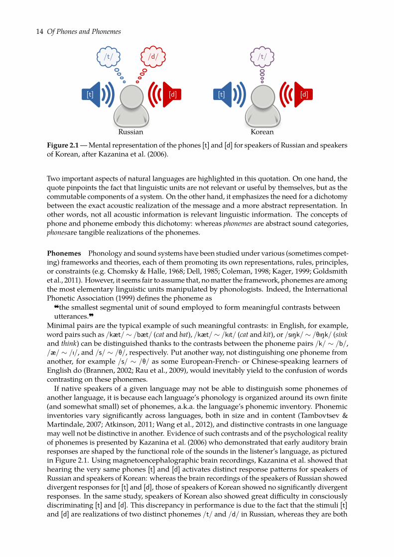
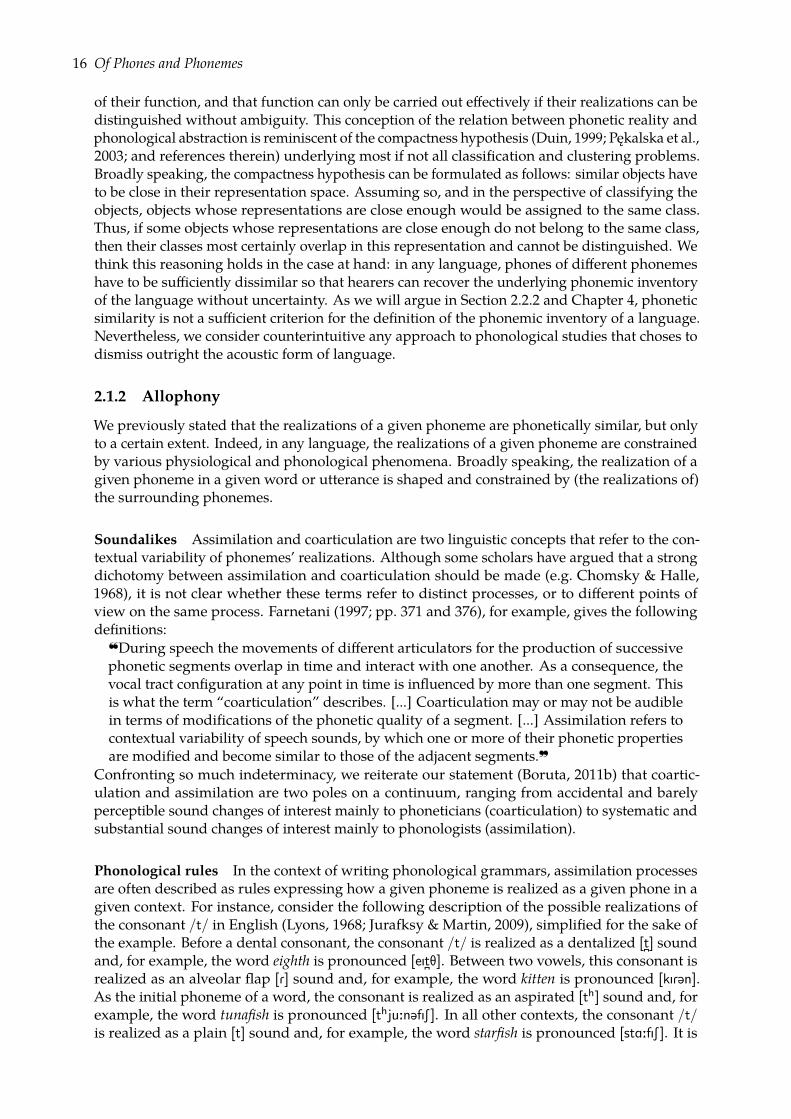
Figure 2.1—Mental representation of the phones [t] and [d] for speakers of Russian and speakersof Korean, after Kazanina et al. (2006).
Two important aspects of natural languages are highlighted in this quotation. On one hand, thequote pinpoints the fact that linguistic units are not relevant or useful by themselves, but as thecommutable components of a system. On the other hand, it emphasizes the need for a dichotomybetween the exact acoustic realization of the message and a more abstract representation. Inother words, not all acoustic information is relevant linguistic information. The concepts ofphone and phoneme embody this dichotomy: whereas phonemes are abstract sound categories,phonesare tangible realizations of the phonemes.
Phonemes Phonology and sound systems have been studied under various (sometimes compet-ing) frameworks and theories, each of them promoting its own representations, rules, principles,or constraints (e.g. Chomsky & Halle, 1968; Dell, 1985; Coleman, 1998; Kager, 1999; Goldsmithet al., 2011). However, it seems fair to assume that, nomatter the framework, phonemes are amongthe most elementary linguistic units manipulated by phonologists. Indeed, the InternationalPhonetic Association (1999) defines the phoneme as
the smallest segmental unit of sound employed to form meaningful contrasts betweenutterances.~
Minimal pairs are the typical example of such meaningful contrasts: in English, for example,word pairs such as /kæt/∼ /bæt/ (cat and bat), /kæt/∼ /kIt/ (cat and kit), or /sINk/∼ /TINk/ (sinkand think) can be distinguished thanks to the contrasts between the phoneme pairs /k/ ∼ /b/,/æ/ ∼ /I/, and /s/ ∼ /T/, respectively. Put another way, not distinguishing one phoneme fromanother, for example /s/ ∼ /T/ as some European-French- or Chinese-speaking learners ofEnglish do (Brannen, 2002; Rau et al., 2009), would inevitably yield to the confusion of wordscontrasting on these phonemes.If native speakers of a given language may not be able to distinguish some phonemes of
another language, it is because each language’s phonology is organized around its own finite(and somewhat small) set of phonemes, a.k.a. the language’s phonemic inventory. Phonemicinventories vary significantly across languages, both in size and in content (Tambovtsev &Martindale, 2007; Atkinson, 2011; Wang et al., 2012), and distinctive contrasts in one languagemay well not be distinctive in another. Evidence of such contrasts and of the psychological realityof phonemes is presented by Kazanina et al. (2006) who demonstrated that early auditory brainresponses are shaped by the functional role of the sounds in the listener’s language, as picturedin Figure 2.1. Using magnetoencephalographic brain recordings, Kazanina et al. showed thathearing the very same phones [t] and [d] activates distinct response patterns for speakers ofRussian and speakers of Korean: whereas the brain recordings of the speakers of Russian showeddivergent responses for [t] and [d], those of speakers of Korean showed no significantly divergentresponses. In the same study, speakers of Korean also showed great difficulty in consciouslydiscriminating [t] and [d]. This discrepancy in performance is due to the fact that the stimuli [t]and [d] are realizations of two distinct phonemes /t/ and /d/ in Russian, whereas they are both
The sounds of language 15
realizations of a single phoneme in Korean, here written as /t/. Indeed, as emphasized by Tobin(1997; p. 314):
native speakers are clearly aware of the phonemes of their language but are both unawareof and even shocked by the plethora of allophones and the minutiae needed to distinguishbetween them.~We previously stated that speakers of English are able to distinguish word pairs such as
/kæt/ ∼ /bæt/ because of the contrast between the phonemes /k/ ∼ /b/. In fact, the reciprocalof this statement may yield a more accurate definition of phonemes as linguistic units: in English,the contrast between sound categories such as /k/∼ /b/ is said to be phonemic because it allowsthe speakers to distinguish word pairs such as /kæt/ ∼ /bæt/. Phonemes do not exist for theirown sake, but for the purpose of producing distinct forms for messages with distinct meanings.
Phones Whereas each language’s sound system comprises a limited number of phonemes, thenumber of phones (a.k.a. speech sounds or segments) is unbounded. Due to many linguisticand extra-linguistic factors such as the speaker’s age, gender, social background, or mood, notwo realizations of the same abstract word or utterance can be strictly identical. Moreover, andnotwithstanding the difficulty of setting phone boundaries (Kuhl, 2004), we define phones asnothing but phoneme-sized chunks of acoustic signal. Thence, as argued by Lyons (1968; p. 100),the concept of phone accounts for a virtually infinite collection of language-independent objects:
The point at which the phonetician stops distinguishing different speech sounds is dictatedeither by the limits of his own capacities and those of his instruments or (more usually) bythe particular purpose of the analysis.~
To draw an analogy with computer science and information theory, phonemes can be thought ofas the optimal lossless compressed representation for human speech. Lossless data compressionrefers to the process of reducing the consumption of resources without losing information,identifying and eliminating redundancy (Wade, 1994; p. 34). In the case of verbal communication,the dispensable redundancy is made of the fine-grained acoustic information that is responsiblefor all conceivable phonetic contrasts, while the true information is made of the language’sphonemic contrasts. Whereas eliminating phonetic contrasts, e.g. [kæt] ∼ [kAt] or [kæt] ∼ [kæ
˚t],
would not result in any loss of linguistic information, no further simplification could be appliedonce the phonemic level has been reached without risking to confuse words, e.g. /kæt/ ∼ /bæt/.The concept of phoneme might be thus defined as the psychological representation for anaggregate of confusable phones. This conception of phonemes as composite constructs hasseldom been emphasized in the literature, though a notable example is Miller (1967; p. 229) who,describing the phonemic inventory of Japanese, denotes as “/i/ the syllabic high front vowels”(emphasis added). The point at which we stop distinguishing different phones in the presentstudy will be presented and discussed in Chapter 3.
Although any phoneme can virtually be realized by an infinite number of distinct phones, theone-to-many relation between sound categories and sound tokens is far from being random orarbitrary. First and foremost, the realizations of a given phoneme are phonetically (or acoustically,we consider both terms to be synonyms) similar, to a certain extent. However, it is worth notingthat the applicability of phonetic similarity as a criterion for the definition of phonemehood hasbeen sorely criticized by theoretical linguists such as Austin (1957; p. 538):
Phonemes are phonemes because of their function, their distribution, not because of theirphonetic similarity. Most linguists are arbitrary and ad hoc about the physical limits ofphonetic similarity.~
On the contrary, we argue in favor of the relevance of phonetic similarity on the grounds that itshould be considered an observable consequence rather than an underlying cause of phoneme-hood. We suggest the following reformulation of the phonetic criterion, already hinted at byMachata & Jelaska (2006): more than the phonetic similarity between the realizations of a givenphoneme, it is the phonetic dissimilarity between the realizations of different phonemes thatmay be used as a criterion for the definition of phonemehood. Phonemes are phonemes because
16 Of Phones and Phonemes
of their function, and that function can only be carried out effectively if their realizations can bedistinguished without ambiguity. This conception of the relation between phonetic reality andphonological abstraction is reminiscent of the compactness hypothesis (Duin, 1999; Pękalska et al.,2003; and references therein) underlying most if not all classification and clustering problems.Broadly speaking, the compactness hypothesis can be formulated as follows: similar objects haveto be close in their representation space. Assuming so, and in the perspective of classifying theobjects, objects whose representations are close enough would be assigned to the same class.Thus, if some objects whose representations are close enough do not belong to the same class,then their classes most certainly overlap in this representation and cannot be distinguished. Wethink this reasoning holds in the case at hand: in any language, phones of different phonemeshave to be sufficiently dissimilar so that hearers can recover the underlying phonemic inventoryof the language without uncertainty. As we will argue in Section 2.2.2 and Chapter 4, phoneticsimilarity is not a sufficient criterion for the definition of the phonemic inventory of a language.Nevertheless, we consider counterintuitive any approach to phonological studies that choses todismiss outright the acoustic form of language.
2.1.2 Allophony
We previously stated that the realizations of a given phoneme are phonetically similar, but onlyto a certain extent. Indeed, in any language, the realizations of a given phoneme are constrainedby various physiological and phonological phenomena. Broadly speaking, the realization of agiven phoneme in a given word or utterance is shaped and constrained by (the realizations of)the surrounding phonemes.
Soundalikes Assimilation and coarticulation are two linguistic concepts that refer to the con-textual variability of phonemes’ realizations. Although some scholars have argued that a strongdichotomy between assimilation and coarticulation should be made (e.g. Chomsky & Halle,1968), it is not clear whether these terms refer to distinct processes, or to different points ofview on the same process. Farnetani (1997; pp. 371 and 376), for example, gives the followingdefinitions:
During speech the movements of different articulators for the production of successivephonetic segments overlap in time and interact with one another. As a consequence, thevocal tract configuration at any point in time is influenced by more than one segment. Thisis what the term “coarticulation” describes. [...] Coarticulation may or may not be audiblein terms of modifications of the phonetic quality of a segment. [...] Assimilation refers tocontextual variability of speech sounds, by which one or more of their phonetic propertiesare modified and become similar to those of the adjacent segments.~
Confronting so much indeterminacy, we reiterate our statement (Boruta, 2011b) that coartic-ulation and assimilation are two poles on a continuum, ranging from accidental and barelyperceptible sound changes of interest mainly to phoneticians (coarticulation) to systematic andsubstantial sound changes of interest mainly to phonologists (assimilation).
Phonological rules In the context of writing phonological grammars, assimilation processesare often described as rules expressing how a given phoneme is realized as a given phone in agiven context. For instance, consider the following description of the possible realizations ofthe consonant /t/ in English (Lyons, 1968; Jurafksy & Martin, 2009), simplified for the sake ofthe example. Before a dental consonant, the consonant /t/ is realized as a dentalized [t”] soundand, for example, the word eighth is pronounced [eIt”T]. Between two vowels, this consonant isrealized as an alveolar flap [R] sound and, for example, the word kitten is pronounced [kIR@n].As the initial phoneme of a word, the consonant is realized as an aspirated [th] sound and, forexample, the word tunafish is pronounced [thju:n@fIS]. In all other contexts, the consonant /t/is realized as a plain [t] sound and, for example, the word starfish is pronounced [stA:fIS]. It is
Early phonological acquisition: state of the art 17
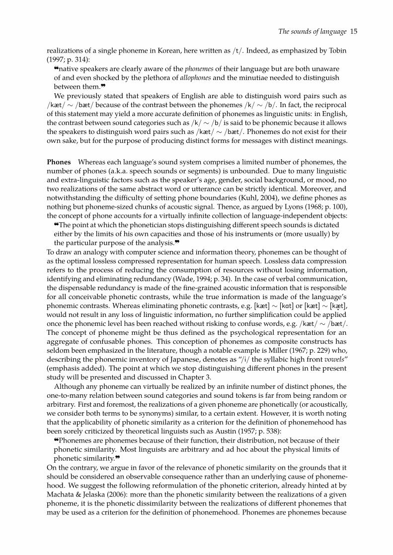
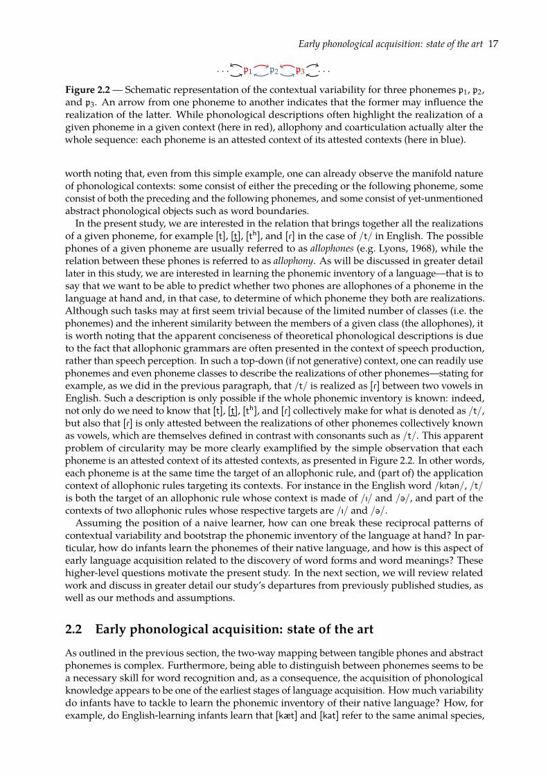
p2p1 p3· · · · · ·Figure 2.2— Schematic representation of the contextual variability for three phonemes p1, p2,and p3. An arrow from one phoneme to another indicates that the former may influence therealization of the latter. While phonological descriptions often highlight the realization of agiven phoneme in a given context (here in red), allophony and coarticulation actually alter thewhole sequence: each phoneme is an attested context of its attested contexts (here in blue).
worth noting that, even from this simple example, one can already observe the manifold natureof phonological contexts: some consist of either the preceding or the following phoneme, someconsist of both the preceding and the following phonemes, and some consist of yet-unmentionedabstract phonological objects such as word boundaries.In the present study, we are interested in the relation that brings together all the realizations
of a given phoneme, for example [t], [t”], [th], and [R] in the case of /t/ in English. The possiblephones of a given phoneme are usually referred to as allophones (e.g. Lyons, 1968), while therelation between these phones is referred to as allophony. As will be discussed in greater detaillater in this study, we are interested in learning the phonemic inventory of a language—that is tosay that we want to be able to predict whether two phones are allophones of a phoneme in thelanguage at hand and, in that case, to determine of which phoneme they both are realizations.Although such tasks may at first seem trivial because of the limited number of classes (i.e. thephonemes) and the inherent similarity between the members of a given class (the allophones), itis worth noting that the apparent conciseness of theoretical phonological descriptions is dueto the fact that allophonic grammars are often presented in the context of speech production,rather than speech perception. In such a top-down (if not generative) context, one can readily usephonemes and even phoneme classes to describe the realizations of other phonemes—stating forexample, as we did in the previous paragraph, that /t/ is realized as [R] between two vowels inEnglish. Such a description is only possible if the whole phonemic inventory is known: indeed,not only do we need to know that [t], [t”], [th], and [R] collectively make for what is denoted as /t/,but also that [R] is only attested between the realizations of other phonemes collectively knownas vowels, which are themselves defined in contrast with consonants such as /t/. This apparentproblem of circularity may be more clearly examplified by the simple observation that eachphoneme is an attested context of its attested contexts, as presented in Figure 2.2. In other words,each phoneme is at the same time the target of an allophonic rule, and (part of) the applicationcontext of allophonic rules targeting its contexts. For instance in the English word /kIt@n/, /t/is both the target of an allophonic rule whose context is made of /I/ and /@/, and part of thecontexts of two allophonic rules whose respective targets are /I/ and /@/.Assuming the position of a naive learner, how can one break these reciprocal patterns of
contextual variability and bootstrap the phonemic inventory of the language at hand? In par-ticular, how do infants learn the phonemes of their native language, and how is this aspect ofearly language acquisition related to the discovery of word forms and word meanings? Thesehigher-level questions motivate the present study. In the next section, we will review relatedwork and discuss in greater detail our study’s departures from previously published studies, aswell as our methods and assumptions.
2.2 Early phonological acquisition: state of the art
As outlined in the previous section, the two-way mapping between tangible phones and abstractphonemes is complex. Furthermore, being able to distinguish between phonemes seems to bea necessary skill for word recognition and, as a consequence, the acquisition of phonologicalknowledge appears to be one of the earliest stages of language acquisition. Howmuch variabilitydo infants have to tackle to learn the phonemic inventory of their native language? How, forexample, do English-learning infants learn that [kæt] and [kat] refer to the same animal species,
18 Of Phones and Phonemes
whereas [kæt] and [bæt] do not? What kind of cues may they rely on to learn that [sINkIN] and[TINkIN] can not refer to the same action?Broadly speaking, research on early language acquisition falls into one of two categories:
behavioral experiments and computational experiments. On one hand, behavioral experimentsare used to assess infants’ response to linguistic stimuli; however, in order to ensure that observedresponses are due solely to the specific linguistic phenomenon studied in the experiment, stimulihave to be thoroughly controlled, and experimental material often consists of synthesized speechor artificial languages. On the other hand, computational experiments allow for the use ofunaltered (yet digitized) natural language. However, conclusions regarding language acquisition(or any other psychological process) drawn from the output of a computer program should beconsidered with all proper reservations, as there is no guarantee that the algorithms and datastructures used in such simulations bear any resemblance to the cognitive processes and mentalrepresentations available to or used by infants. Because of this trade-off between the ecologicalvalidity of the learner and that of the learning material, in vivo and in silico experiments arecomplementary approaches for research on language acquisition. The outline of this sectionfollows this dichotomy: we will first provide a brief review of behavioral results in order to setthe scene, and we will then review computational results in order to discuss how our studydeparts from previously reported research efforts.
Babies, children and infants Throughout this study, young human learners will be uniformlyreferred to as infants, mainly because of the word’s latin etymology, infans, meaning “not able tospeak.” We henceforth use infant-directed speech as an umbrella term for motherese, child-directedspeech, or any other word used to describe infants’ linguistic input.It is also worth emphasizing immediately that, for the sake of simplicity, the present study
focuses on early language acquisition in a monolingual environment. As interesting as bi- orplurilingualism may be, learning the phonemic inventory of a single language is a dauntingenough task, as we will explain in the rest of this study.
2.2.1 Behavioral experiments
Although an extensive review of the literature on early language acquisition would require amonograph of its own, we will here review the major results in the field, focusing on speechperception and the emergence of phonemes. Furthermore, and for the sake of simplicity, we willmainly give references to a small number of systematic reviews (Plunkett, 1997; Werker & Tees,1999; Peperkamp, 2003; Clark, 2004; Kuhl, 2004), rather than to all original studies. For a reviewfocusing on the acquisition of speech production, see Macneilage (1997).
Cracking the speech code Remarkable results about infants’ innate linguistic skills have high-lighted their ability to discriminate among virtually all phones, including those illustratingcontrasts between phonemes of languages they have never heard (Kuhl, 2004). Nevertheless,some adaptation to their native language’s phonology occurs either in utero or immediately afterbirth; indeed, it has been observed that infants aged 2 days show a preference for listening to theirnative language (Werker & Tees, 1999). Afterwards, exposure to a specific language sharpensinfants’ perception of the boundaries between the phonemic categories of that language. Forexample, English-learning infants aged 2–4 months are able to perceptually group realizations ofthe vowel /i/ uttered by a man, woman, or child in different intonative contexts, distinguishingthese phones from realizations of the vowel /a/ (Werker & Tees, 1999). As they improve theirknowledge of their native language’s phonology, infants also gradually lose the ability to dis-criminate among all phones. While it has been shown, for instance, that English-learning infantsaged 6–8 months are able to distinguish the glottalized velar vs. uvular stop contrast [k’] ∼ [q’]in Nthlakapmx, a Pacific Northwest language, this ability declines after the age of 10–12 months(Plunkett, 1997). It is also worth noting that, throughout the course of language acquisition,
Early phonological acquisition: state of the art 19
infants learn not only the phonemes of their native language, but also how to recognize thesephonemes when uttered by different speakers and in different contexts (Kuhl, 2004), a taskthat has proven to be troublesome for computers (e.g. Woodland, 2001). As a whole, learningphonemes can be thought of as learning not to pay attention to (some) detail.
Stages of interest in Kuhl’s (2004) universal timeline of speech perception development canbe summarized as follows. From birth to the age of 5 months, infants virtually discriminatethe phonetic contrasts of all natural languages. Then, language-specific perception begins totake place for vowels from the age of 6 months onwards. This is also the time when statisticallearning can first be observed, most notably from distributional frequencies. The age of 8 monthsmarks a strong shift in the transition from universal to language-specific speech perception:now also relying on transitional probabilities, infants are able to recognize the prosody (viz. thetypical stress patterns) and the phonotactics (i.e. the admissible sound combinations) of theirnative language. From the age of 11 months onwards, infants’ sensitivity to the consonants oftheir native language increases, at the expense of the (universal) sensitivity to the consonantsin foreign languages. Finally, infants master the major aspects of the grammar of their nativelanguage by the age of 3 years (Peperkamp, 2003).
Statistical learning Infants’ ability to detect patterns and regularities in speech is often referredto as statistical learning, i.e. the acquisition of knowledge through the computation of informationabout the distributional frequency of certain items, or probabilistic information in sequencesof such items (Kuhl, 2004). In particular under a frequentist interpretation of probabilities(Hájek, 2012), this appealing learning hypothesis is corroborated by various experiments wherelanguage processing has been showed to be, in adults as in infants, intimately tuned to frequencyeffects (Ellis, 2002). Virtually all recent studies on early language acquisition whose models orassumptions rely on statistical learning build upon the seminal studies by Saffran et al. whoshowed that 8-month-old infants were able to segment words from fluent speech making onlyuse of the statistical relations between neighboring speech sounds, and after only two minutesof exposure (Saffran et al., 1996; Aslin et al., 1998; Saffran, 2002). However, as emphasized byKuhl (2004; pp. 831–832), infants’ learning abilities are also highly constrained:
Infants can not perceive all physical differences in speech sounds, and are not computa-tional slaves to learning all possible stochastic patterns in language input. [...] Infants donot discriminate all physically equal acoustic differences; they show heightened sensitivityto those that are important for language.~
Although it would be beyond the stated scope of this research to enter into the debate of naturevs. nurture, it is worth noting that various authors have proposed that the development of speechperception should be viewed as an innately guided learning process (Jusczyk & Bertoncini,1988; Gildea & Jurafsky, 1996; Plunkett, 1997; Bloom, 2010). Bloom, for instance, highlights thisapparent predisposition of infants for learning natural languages as follows:
One lesson from the study of artificial intelligence (and from cognitive science moregenerally) is that an empty head learns nothing: a system that is capable of rapidly absorbinginformation needs to have some prewired understanding of what to pay attention to andwhat generalizations to make. Babies might start off smart, then, because it enables them toget smarter.~
Furthermore, as prominent as Saffran et al.’s (1996) results may be, they should not be overinter-preted. Although it is a necessity for experimental studies to use controlled stimuli, it is worthpointing out that the stimuli used by Saffran et al. consisted in four three-syllable nonsense words(viz. /tupiro/, /bidaku/, /padoti/, and /golabu/ for one of the two counterbalanced conditions)whose acoustic forms were generated by a speech synthesizer in a monotone female voice at aconstant rate of 270 syllables per minute. As stated by the authors, the only cue to word bound-aries in this artificial language sample were the transitional probabilities between all syllablepairs. By contrast, natural infant-directed speech contains various cues to different aspects ofthe language’s grammar: stress, for example, is one of many cues for the discovery of word
20 Of Phones and Phonemes
boundaries in various languages, and it has been shown to collide with statistical regularities in(more plausible) settings where infants have to integrate multiple cues (Johnson & Jusczyk, 2001;Thiessen & Saffran, 2003). Additionally, not all statistically significant co-occurrence patterns arerelevant cues for learning the grammar of either the language at hand or, possibly, any otherlanguage. Indeed, as emphasized by Gambell & Yang (2004; p. 50):
While infants seem to keep track of statistical information, any conclusion drawn fromsuch findings must presuppose children knowing what kind of statistical information tokeep track of. After all, an infinite range of statistical correlations exists in the acoustic input:e.g., What is the probability of a syllable rhyming with the next? What is the probability oftwo adjacent vowels being both nasal?~
In the present study, we endorse the aforementioned views that the development of speechperception is an innately guided learning process and that statistical learning is a key componentof early language acquisition. The following section reviews previously published modelingefforts with the aim of making each study’s major assumptions explicit, thus specifying how thisstudy departs from the state of the art.
2.2.2 Computational experiments
As noted by Peperkamp (2003), experimental research on speech perception has shown a strongfocus on the acquisition and the mental representation of phonemes and allophones. Unfortu-nately, this observation does not hold for computational studies. Indeed, while a limited numberof studies attempting to model how infants may learn the phonemes of their native languagehave been reported so far, a tremendous number of studies on the acquisition of word segmenta-tion strategies have been published (e.g. Olivier, 1968; Elman, 1990; Brent & Cartwright, 1996;Christiansen et al., 1998; Brent, 1999; Venkataraman, 2001; Johnson, 2008b; Goldwater et al., 2009;Pearl et al., 2010; to cite but a few). In our opinion, this ongoing abundance of computationalmodels and experiments on word segmentation is due to the fact that merely splitting sequencesof characters requires more skills in stringology than in psychology or linguistics. Indeed, untilvery recently (Rytting et al., 2010; Daland & Pierrehumbert, 2011; Boruta et al., 2011; Elsner et al.,2012), most—if not all—models of word segmentation have used idealized input consisting inphonemic transcriptions and, as we have argued in a previous study (Boruta et al., 2011; p. 1):
these experiments [...] make the implicit simplifying assumption that, when children learnto segment speech into words, they have already learned phonological rules and know howto reduce the inherent variability in speech to a finite (and rather small) number of abstractcategories: the phonemes.~
The ultimate goal of the project reported in the present study is to develop and validate acomputational model of the acquisition of phonological knowledge that would precisely accountfor this assumption, mapping each phone to the phoneme of which it is a realization.Before reviewing related work, it is worth emphasizing immediately that the present study
departs from most research efforts on allophony and sound variability on one major point: weare interested in gaining valuable insights on human language and human language acquisition.Although our results were obtained through computational experiments, we have for this reasonlittle interest for performance-driven methods for phoneme recognition, as developed and usedin the field of automatic speech recognition (e.g. Waibel et al., 1989; Matsuda et al., 2000; Schwarzet al., 2004; Huijbregts et al., 2011). By contrast, our subject matter is language and, thence, thepresent study is to be considered a contribution to data-intensive experimental linguistics, in thesense of Abney (2011).
Related work Research efforts on models of the acquisition of phonology have been ratherscarce and uncoordinated: to our knowledge, no shared task or evaluation campaign has everbeen organized on such topics, while different studies have seldom used the same data oralgorithms. We will briefly review previously published models in this section, highlighting the
Early phonological acquisition: state of the art 21
similarities and discrepancies between them and the present study. For general discussions ofcategory learning and phonological acquisition, see Boersma (2010) and Ramus et al. (2010).At the pinnacle of structuralism, Harris (1951, 1955) presented a procedure for the discovery
of phonemes (and other linguistic units) that relies on successor counts, i.e. on the distributionalproperties of phones within words or utterances in a given language. Unfortunately, this discov-ery procedure is only meant to be applied by hand as too many details (e.g. concerning datarepresentation or the limit of phonetic similarity) were left unspecified as to be able to implementand validate a full computational model.To our knowledge, the first complete algorithms capable of learning allophonic rules were
proposed by Johnson (1984), Kaplan & Kay (1994) and Gildea & Jurafsky (1996): all threealgorithms examine the machine learning of symbolic phonological rules à la Chomsky &Halle (1968). However, as noted by Gildea & Jurafsky, these algorithms include no mechanismto account for the noise and the non-determinism inherent to linguistic data. An additionallimitation of Gildea & Jurafsky’s algorithm is that it performs supervised learning, i.e. it requiresa preliminary training step during which correct pairs of phonetic and phonological formsare processed; yet, performing unsupervised learning is an essential plausibility criterion forcomputational models of early language acquisition (Brent, 1999; Alishahi, 2011; Boruta et al.,2011) as infant-directed speech does not contain such ideal labeled data.A relatively high number of models of the acquisition of phonological knowledge (Tesar &
Smolensky, 1996; Boersma & Levelt, 2000, 2003; Boersma et al., 2003; Hayes, 2004; Boersma, 2011;Magri, 2012) have been developed in the framework of optimality theory (Prince & Smolensky,1993; Kager, 1999). Tesar & Smolensky’s (1996) model, for instance, is able to learn both themapping from phonetic to phonological forms and the phonotactics of the language at hand.It is however worth mentioning that optimality-theoretic models make various non-trivialassumptions—viz. regarding the availability of a phonemic inventory, distinctive features, wordsegmentation, and a mechanism recovering underlying word forms from their surface forms.For this reason, such models are not comparable with the work presented in this dissertation, aswe specifically address the question of the acquisition of a given language’s phonemic inventory.
In an original study, Goldsmith & Xanthos (2009) addressed the acquisition of higher-levelphonological units and phenomena, namely the pervasive vowel vs. consonant distinction, vowelharmony systems, and syllable structure. Doing so, they assume that the phonemic inventoryand a phonemic representation of the language at hand are readily available to the learner.Goldsmith & Xanthos’ matter of concern is hence one step ahead of ours.Building upon a prior theoretical discussion that infants may be able to undo (some) phono-
logical variation without having acquired a lexicon (Peperkamp & Dupoux, 2002), Peperkampet al. have developed across various studies a bottom-up, statistical model of the acquisitionof phonemes and allophonic rules relying on distributional and, more recently, acoustic andproto-lexical cues (Peperkamp et al., 2006; Le Calvez, 2007; Le Calvez et al., 2007; Dautriche,2009; Martin et al., 2009; Boruta, 2009, 2011b). Revamping Harris’ (1951) examination of everyphone’s attested contexts, Peperkamp et al.’s (2006) distributional learner looks for pairs ofphones with near-complementary distributions in a corpus. Because complementary distribu-tions is a necessary but not sufficient criterion, the algorithm then applies linguistic constraints todecide whether or not two phones are realizations of the same phoneme, checking, for example,that potential allophones share subsegmental phonetic or phonological features (cf. Gildea &Jurafsky’s faithfulness constraint). Further developments of this model include replacing apriori faithfulness constraints by an empirical measure of acoustic similarity between phones(Dautriche, 2009), and examining infants’ emerging lexicon (Martin et al., 2009; Boruta, 2009,2011b). Consider, for example, the allophonic rule of voicing in Mexican Spanish, as presentedby Le Calvez et al. (2007), by which /s/ is realized as [z] before voiced consonants (e.g. felizNavidad, “happy Christmas,” is pronounced as [feliz nabidad], ignoring other phonological pro-cesses for the sake of the example) and as [s] elsewhere (e.g. feliz cumpleaños, “happy birthday,”is pronounced as [felis kumpleaños]). Although it introduces the need for an ancillary word
22 Of Phones and Phonemes
segmentation procedure, Martin et al. (2009) showed that tracking alternations on the first orlast segment of otherwise identical word forms such as [feliz] ∼ [felis] (which are not minimalpairs stricto sensu) is a relevant cue in order to learn allophonic rules.
Except for Dautriche’s (2009) extension of Peperkamp et al.’s model, a stark limitation ofall aforementioned models is that they operate on transcriptions, and not on sounds. As weargued in a previous study (Boruta, 2011b), phones are nothing but abstract symbols in suchapproaches to speech processing, and the task is as hard for [a] ∼ [a
˚] as it is for [4] ∼ [k]. Despite
the fact that formal language theory has been at the heart of computational linguistics and,especially, computational phonology (Kaplan & Kay, 1994; Jurafksy & Martin, 2009; Wintner,2010; and references therein), we reiterate our argument that legitimate models of the acquisitionof phonological knowledge should not disregard the acoustic form of language.Several recent studies have addressed the issue of learning phonological knowledge from
speech: while Yu (2010) presented a case study with lexical tones in Cantonese, Vallabha et al.(2007) and Dillon et al. (2012) focused on learning phonemic categories from English or Japaneseinfant-directed speech and adult-directed Inuktitut, respectively. However, in all three studies,the linguistic material used as the models’ input was hand-annotated by trained phoneticians,thus hindering the reproducibility of these studies. Furthermore, and even if a model canonly capture certain aspects of the process of language acquisition, highlighting some whilemuting others (Yu, 2010; p. 11), both studies attempting to model the acquisition of phonemesrestricted the task to the acquisition of the vowels of the languages at hand (actually a subset ofthe vowel inventories in Vallabha et al.’s study). Although experimental studies have suggestedthat language-specific vowel categories might emerge earlier than other phonemes (Kuhl, 2004;and references therein), we consider that the phonemic inventory of any natural language is acohesive and integrative system that can not be split up without reserve. These computationalstudies offer interesting proof of concepts, but they give no guarantee as to the performanceof their respective models in the (plausible) case in which the learner’s goal is to discover thewhole phonemic inventory.
The overall goal of the present study is to build upon Peperkamp et al.’s experiments to proposea model of the acquisition of phonemes that supplements their distributional learner (Peperkampet al., 2006; Le Calvez, 2007; Le Calvez et al., 2007; Martin et al., 2009; Boruta, 2009, 2011b) withan examination of available acoustic information (Vallabha et al., 2007; Dautriche, 2009; Dillonet al., 2012). To do so, we introduce a (somewhat artificial) dichotomy between the conceptsof allophony and phonemehood, mainly because of the discrepancies between the state of theart and the aim of this project: whereas Peperkamp et al. have focused on predicting whethertwo phones are realizations of the same phoneme (what we will refer to as allophony), we areeventually interested in predicting which phoneme they both are realizations of (what we willrefer to as phonemehood). Bridging, to some extent, the gap between symbolic (i.e. phonology-driven) and numeric (i.e. phonetics-driven) approaches to the acquisition of phonology, we willalso address the issue of the limits of phonetic similarity by evaluating our model with dataundergoing different degrees of phonetic and phonological variability.
Models of the humanmind Cognitivemodeling and so called psychocomputational models oflanguage acquisition have received increasing attention in the last decade, as shown by the emer-gence (and continuance) of specialized conferences and workshops such as Cognitive Modelingand Computational Linguistics (CMCL), Psychocomputational Models of Human Language Acquisition(PsychoCompLA), or Architectures and Mechanisms for Language Processing (AMLaP). Because ofthe diversity in linguistic phenomena, theories of language acquisition, and available modelingtechniques, developing computational models of early language acquisition is an intrinsicallyinterdisciplinary task. Though computational approaches to language have sometimes beencriticized by linguists (e.g. Berdicevskis & Piperski, 2011), we nonetheless support Abney’s (2011)argumentation that data-intensive experimental linguistics is genuine linguistics, and we willhereby discuss the major points that distinguish a computational model of language processing
Early phonological acquisition: state of the art 23
from a linguistic theory.The objection that our conclusions are merely drawn from the output of a computer program
(rather than from observed behavioral responses) was raised various times during early pre-sentations of the work reported in this dissertation. Although this is true, by definition, of anycomputational study, it is not a strong argument, as pointed out by Hodges (2007; pp. 255–256;see also the discussion by Norris, 2005):
The fact that a prediction is run on a computer is not of primary significance. The validityof the model comes from the correctness of its mathematics and physics. Making predictionsis the business of science, and computers simply extend the scope of human mental facultiesfor doing that business. [...] Conversely, if a theory is wrong then running it on a computerwon’t make it come right.~
We nevertheless concede that a major issue faced by computational linguists is that our linguisticmaterial is not the kind of data that computers manipulate natively: while, broadly speaking,linguists are interested in sounds and words, computers only manipulate zeros and ones. Hence,to the bare minimum, the speech stream needs to be digitized; phones are represented as vectors,and words as sequences of such vectors. Put another way, words fly away, while numbers remain.Depending on the chosen numerical representation, adapting or transforming the input is notwithout consequences, as noted by Pękalska & Duin (2005; p. 163):
Such a simplification of an object to its numerical description (i.e. without any structuralinformation) precludes any inverse mapping to be able to retrieve the object itself.~
Therefore, throughout this study, a special emphasis will be put on discussing how phones andphonemes are represented in our simulations, as well as how these representations may impactthe performance of the models.
In addition to data representation, working hypotheses andmodeling assumptions are anotherpitfall for computational linguists. Indeed, an algorithm may impose preconditions on the inputdata (e.g. requirements for statistical independence of the observations, a given probabilitydistribution, or a minimum number of observations). Different algorithms solving the sameproblem may impose different preconditions on the data and, if one or more preconditions areviolated (or arbitrarily waived), the behavior of an algorithm may become flawed or unspecified.A potential issue lies in the fact that not all preconditions can be verified automatically: binomiallogistic regression, for example, assumes that the observations are independent (i.e. the outcomefor one observation does not affect the outcome for another; Agresti, 2007; p. 4), but this propertycan not be verified without expert knowledge, and any implementation would be able to fita binomial logistic regression model to some observations, no matter whether they are trulyindependent or not. In other words, the correctness of the program does not guarantee thecorrectness of the experiment, thus illustrating the previous quotation from Hodges (2007).Furthermore, making assumptions explicit is a methodological advantage of computationalmodels over theories, as argued by Alishahi (2011; p. 5):
This property distinguishes a computational model from a linguistic theory, which nor-mally deals with higher-level routines and does not delve into details, a fact that makes suchtheories hard to evaluate.~
This discrepancy may be reformulated in terms of Marr’s (1982) levels of analysis. Whereaslinguistic theories may only probe the computational level (i.e. a description of the problemand of the global logic of the strategy used to solve it), computational models must provide athorough and extensive discussion of the algorithmic level (i.e. a description of the operatedtransformations and of the representations for the input and the output). The last level, viz. theimplementation level, is beyond the stated scope of this research as it describes how the systemis physically realized and thus, in the case at hand, belongs to the field of neurolinguistics.For the aforementioned reasons, a special emphasis will also be put on making modeling
assumptions explicit throughout this study, highlighting them in the way that proofs or theo-rems are often highlighted in mathematics. For instance, we have already made the followingassumptions through the course of this chapter:

24 Of Phones and Phonemes
Assumption 2.1 The development of speech perception by infants is neither fully innate norfully acquired, but an innately guided learning process (cf. Jusczyk & Bertoncini, 1988; Gildea &Jurafsky, 1996; Plunkett, 1997; Bloom, 2010).
Assumption 2.2 Phonological processes only involve two levels of representation: the underly-ing, phonemic level and the surface, phonetic level (cf. Koskenniemi, 1983; Kaplan & Kay, 1994;Coleman, 1998).
Assumption 2.3 Phoneme-sized units are employed at all stages of phonological encoding anddecoding (cf. Ohala, 1997).
Assumption 2.4 Infants are innately able to segment the stream of speech into phoneme-sizedunits (cf. Peperkamp et al., 2006; Le Calvez, 2007).
Assumption 2.5 Infants are good statistical learners and are able to monitor, for example, phonefrequencies or transition probabilities between phones (cf. Saffran et al., 1996; Aslin et al., 1998;Saffran, 2002; Kuhl, 2004).
Assumption 2.6 Allophony and coarticulation processes can be reduced to strictly local, sound-altering processes that yield no segmental insertion or deletion (cf. Le Calvez, 2007; Goldsmith& Xanthos, 2009).
Assumption 2.7 Infants are able to undo (some) phonological variation without having yetacquired an adult-like lexicon (cf. Peperkamp & Dupoux, 2002; Peperkamp et al., 2006; Martinet al., 2009).
Assumption 2.8 Infants are able to acquire the phonemic inventory of their native languagewithout knowledge of any other phonological construct such as features, syllables, or foots (cf.Le Calvez, 2007; Goldsmith & Xanthos, 2009; Boersma, 2010).
CHAPTER 3SOURCES OF DATA
The aim of this chapter is to present the corpus of Japanese used throughout the present study,and to report all preprocessing steps applied to this master dataset. We also give an overviewof the principles involved in deriving the allophonic rules whose modeling and acquisition arediscussed in subsequent chapters. The focus is on presenting the similarities and discrepanciesbetween our data-driven allophonic rules and traditional, theoretical descriptions of allophony inJapanese. It is worth highlighting immediately that, contrary to other chapters, the methodologydiscussed and used in this chapter is to a certain extent specific to the particular dataset we used:replacing this corpus with another one should yield no loss in the generality of the models tobe further described except, obviously, with regard to conclusions drawn from quantitative orqualitative evaluations of the models’ performance.
This chapter is divided into three main sections. Section 3.1 contains a general description ofthe corpus we used. In Section 3.2, we discuss how we derived allophones and allophonic rulesfrom this corpus, aswell as themechanismswe used to control the limits of the phonetic similaritybetween the allophones of a given phoneme. Finally, Section 3.3 contains an examination of howour data eventually relate to theoretical descriptions of the phonology of Japanese.
3.1 The Corpus of Spontaneous Japanese
The corpus we used throughout this study to develop and validate our models is the Corpusof Spontaneous Japanese (henceforth CSJ; Maekawa et al., 2000; Maekawa, 2003), a large-scaleannotated corpus of Japanese speech. The whole CSJ contains about 650 hours of spontaneousspeech (corresponding to about 7 million word tokens) recorded using head-worn, close-talkingmicrophones and digital audio tapes, and down-sampled to 16 kHz, 16 bit accuracy (CSJ Website,2012). There is a true subset of the CSJ, referred to as the Core, which contains 45 hours of speech(about half a million words); it is the part of the corpus to which the cost of annotation wasconcentrated and, as a matter of fact, the only part where segment labels (i.e. phonetic andphonemic annotations) are provided. Therefore, from this point on, all mentions of the CSJ referto the Core only.
On using the CSJ Although, for the sake (no pun intended) of brevity, we only report experi-ments using Japanese data in the present study, our goal is to develop a language-independent(dare we say, universal) computational model of the early acquisition of allophony and phoneme-hood. In other words, the models to be presented in subsequent chapters were not tuned to thisspecific corpus of Japanese, nor to any property of the Japanese language. Despite the fact thatit has been argued, including by us, that computational models of early language acquisitionshould be evaluated using data from typologically different languages in order to assess their
26 Sources of Data
sensitivity to linguistic diversity (Gambell & Yang, 2004; Boruta et al., 2011), we leave this as arecommendation for future research.A more arguable choice was to use adult-directed speech as input data for models of early
language acquisition. Notwithstanding the ongoing debate about how infant-directed speechmight differ from adult-directed speech (Kuhl, 2004; Cristia, 2011), using infants’ linguistic inputto model infants’ linguistic behavior would have been a natural choice. However, in the caseat hand, our choice was constrained by the limited availability of transcribed speech databases.Indeed, to our knowledge, no database of infant-directed speech with aligned phonemic tran-scriptions was available in 2009, when the work reported in the present study was initiated. Inany case, we follow Daland & Pierrehumbert’s (2011) discussion, presented hereafter, concerningthe relevance of using adult-directed speech as input data to models of early language acquisition.Would infant-directed speech be no different from adult-directed speech, then all conclusionsdrawn from the models’ performance on the CSJ could be drawn for the acquisition of Japanesewithout loss of generality. On the contrary, would infant-directed speech indeed be differentfrom adult-directed speech, and because studies supporting this alternative have argued thatinfant-directed speech is hyperarticulated in order to facilitate language acquisition (Kuhl, 2004;and references therein), then our models would have been evaluated in a worst case scenario.
A word about reproducibility Unfortunately, the CSJ is not freely available. Nonethe-less, in order to guarantee the reproducibility of the work reported in this study, all pro-grams and derivative data were made available to the community on a public repository athttp://github.com/lucboruta.Our concern for reproducibility also dictated the level of detail in this chapter, as well as
our decision to report preprocessing operations from the beginning of this study, rather thanin an appendix. Indeed, as will be further mentioned, ambiguous linguistic compromises orunspecified implementation choices have proven to hinder the repeatability of and comparabilitywith previously reported experiments (viz. Dautriche, 2009; Martin et al., 2009).
3.1.1 Data preprocessing
Speech data in the CSJ were transcribed and annotated on various linguistic levels including,but not limited to, phonetics, phonology, morphology, syntax, and prosody. As the presentstudy focuses on lower linguistic levels, the rich XML-formatted transcripts of the CSJ werepreprocessed to extract information about phonemes, words, and (loosely defined) utterances.In order to train sound and accurate acoustic models, the focus of the preprocessing operationswas on removing non-speech passages, as well as keeping track of temporal annotations so thatthe modified transcripts could still be aligned with the original audio recordings. Moreover, it isworth mentioning that although Dautriche (2009), too, used the CSJ, our data were extractedfrom newer, updated transcripts of the corpus.
Phonemes As previously stated, wewant to address the issue of the limits of phonetic similarity,that is to say we want to control how varied and detailed our phonetic input will be. To do so,we follow a method initiated by Peperkamp et al. (2006) that we further systematized (Boruta,2009, 2011a,b; Boruta et al., 2011): we created phonetic transcriptions by applying allophonicrules to a phonemically transcribed corpus. The particular technique we used in this study ispresented in Section 3.2; here, our goal is to remove all phonetic annotations in the CSJ in orderto obtain our initial phonemically transcribed corpus.
In the XMLmarkup of the corpus, segmental data were annotated using two distinct elements:Phone and Phoneme. However, despite the names, a Phoneme element is made of one or moreembedded Phone elements, and Phone elements may actually describe subsegmental events suchas creakiness at the end of a vowel, or voicing that continues after the end of a vowel’s formants(CSJ DVD, 2004). Therefore, we extracted the information about a phone’s underlying phonemic
The Corpus of Spontaneous Japanese 27
category from the PhonemeEntity attribute of the Phoneme element. As Phoneme elements do notinclude temporal annotations, we derived the timestamps of a phoneme from the timestampsof the contained Phone elements: the extracted starting timestamp of a phoneme is the startingtimestamp of its first Phone and, mutatis mutandis, the ending timestamp of a phoneme is theending timestamp of its last Phone.
Words The word segmentation and part-of-speech analyses of the CSJ were conducted for twodifferent kinds of words: short-unit words (annotated as SUW) and long-unit words (annotated asLUW), which are defined as follows (CSJ Website, 2012):
Most of the SUW are mono-morphemic words or words made up of two consecutive mor-phemes, and approximate dictionary items of ordinary Japanese dictionaries. LUW, on theother hand, is for compounds.~
Therefore, what will from this point on be referred to as words were extracted from the SUW tags.Moreover, the content of a given word was made up as the sequence of all embedded Phonemeelements, ignoring intermediate XML elements such as TransSUW or Mora, if any.
Utterances In the CSJ annotations, utterances are defined as inter-pausal units (tagged as IPU).According to the documentation, an utterance is a speech unit bounded by pauses of morethan 200 ms (CSJ DVD, 2004). Nonetheless, extracting utterances and utterances’ content isnot a straightforward process as Noise tags were used as that level, too, to annotate unintelli-gible passages as well as anonymized data. Thence, an IPU element can be broken down intoa sequence of one or more chunks; each chunk being either noise or workable words. Fur-ther annotation of such noise chunks in terms of words and phonemes is often incomplete,if not inexistent. It is also worth noting that, in the recordings, the audio passages matchingsome Noise elements were covered with white noise, so that looking past Noise tags (as didDautriche, 2009) would surely compromise the training of acoustics-based models. For these rea-sons, all Noise chunks were discarded during preprocessing. For instance, an hypothetical IPUof the form <IPU><SUW>...</SUW><Noise>...</Noise><SUW>...</SUW><SUW>...</SUW></IPU>would be extracted as two distinct utterances: one containing only the first word, the othercontaining the two words appearing after the Noise chunk (unfortunately, the XML annotationsare too rich and verbose so that an actual example could be presented on a single page).
In order to detect inconsistent annotations and to ensure the quality and the coherence of theextracted corpus, we performed various sanity checks, discarding utterance chunks that did notmeet the following criteria:— utterance chunks must contain at least one word;— words must contain at least one phoneme;— within a word, the ending timestamp of a phoneme must match the starting timestamp of
the following phoneme;— phonemes’ timestamps must denote strictly positive durations;— utterance chunks must be at least 100 ms-long, a threshold suggested by Dupoux & Schatz
(priv. comm.).Further modifications were applied, on the basis of the labels of some phoneme-level units; theyare reported in the following section, together with a summary of all deletions in Table 3.1.
3.1.2 Data-driven phonemics
Completing the preprocessing operations described in the previous section yields a corpusreduced to three-level data: utterances that are made up of words that are made up of phonemes.Additional preprocessing is however necessary in order to obtain true phonemic transcriptions.The reason for this is twofold. On one hand, the categories gathered from the PhonemeEntityattributes do not only denote phonemic contrasts, but also allophonic contrasts. On the otherhand, some phonemes of the inventory used in the CSJ are heavily under-represented and, in
28 Sources of Data
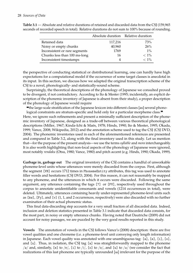
Table 3.1—Absolute and relative durations of retained and discarded data from the CSJ (159,965seconds of recorded speech in total). Relative durations do not sum to 100% because of rounding.
Absolute duration Relative duration
Retained data 117,216 73%Noisy or empty chunks 40,960 26%Inconsistent or rare segments 1769 1%Chunks less than 100 ms-long 16 < 1%Inconsistent timestamps 4 < 1%
the perspective of conducting statistical or distributional learning, one can hardly have highexpectations for a computational model if the occurrence of some target classes is anecdotal inits input. In this section, we discuss how we adapted the original transcription scheme of theCSJ to a novel, phonologically- and statistically-sound scheme.Surprisingly, the theoretical descriptions of the phonology of Japanese we consulted proved
to be divergent, if not contradictory. According to Ito & Mester (1995; incidentally, an explicit de-scription of the phonemic inventory of Japanese is absent from their study), a proper descriptionof the phonology of Japanese would require
the large-scale stratification of the Japanese lexicon into different classes [as] several phono-logical constraints are stratum-specific and hold only for a particular morpheme class.~
Here, we ignore such refinements and present a minimally sufficient description of the phone-mic inventory of Japanese, designed as a trade-off between various theoretical phonologicaldescriptions (Miller, 1967; Kinda-Ichi & Maës, 1978; Hinds, 1990; Ito & Mester, 1995; Okada,1999; Vance, 2008; Wikipedia, 2012) and the annotation scheme used to tag the CSJ (CSJ DVD,2004). The phonemic inventories used in each of the aforementioned references are presentedand compared in Table 3.2, along with the final inventory used in this study. Let us mentionthat—for the purpose of the present analysis—we use the terms syllable andmora interchangeably.It is also worth highlighting that non-local aspects of the phonology of Japanese were ignored,most notably rendaku (Otsu, 1980; Vance, 1980) and pitch accent (e.g. Hinds, 1990; Okada, 1999).
Garbage in, garbage out The original inventory of the CSJ contains a handful of unworkablephoneme-level units whose utterances were merely discarded from the corpus. First, althoughthe segment [VN] occurs 1712 times in PhonemeEntity attributes, this tag was used to annotatefiller words and hesitations (CSJ DVD, 2004). For this reason, it can not reasonably be mappedto any phoneme, and the utterances in which it occurs were discarded. Following the sameargument, any utterance containing the tags [?] or [FV], respectively used throughout thecorpus to annotate unidentifiable consonants and vowels (1214 occurrences in total), weredeleted. Ultimately, utterances containing heavily under-represented phoneme-level units suchas [kw], [Fy], and [v] (1, 1, and 2 occurrences, respectively) were also discarded with no furtherexamination of their actual phonemic status.
This final data-discarding step accounts for a very small fraction of all discarded data. Indeed,inclusion and deletion statistics presented in Table 3.1 indicate that discarded data consists, forthe most part, in noisy or empty utterance chunks. Having noted that Dautriche (2009) did notaccount for noisy passages, we are puzzled by the very good results reported in this study.
Vowels The annotation of vowels in the CSJ follows Vance’s (2008) description: there are fivevowel qualities and one chroneme (i.e. a phoneme-level unit conveying only length information)in Japanese. Each vowel quality was annotated with one unambiguous tag: [a], [e], [i], [o],and [u]. Thus, in isolation, the CSJ tag [a] was straightforwardly mapped to the phoneme/a/ and, similarly, [e] to /e/, [i] to /i/, [o] to /o/, and [u] to /u/ (we consider the fact thatrealizations of this last phoneme are typically unrounded [W] irrelevant for the purpose of the
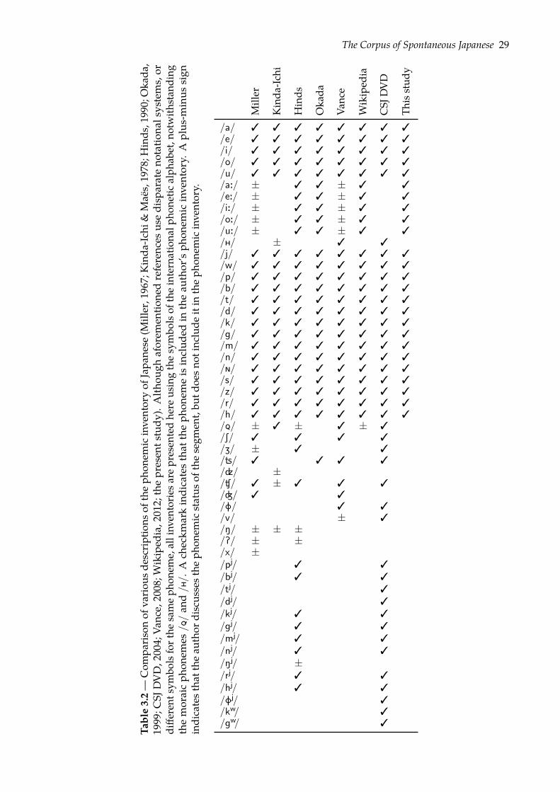
The Corpus of Spontaneous Japanese 29
Table3.2—
Com
paris
onof
vario
usde
scrip
tions
oftheph
onem
icinve
ntoryof
Japa
nese
(Miller,1967;Kinda
-Ichi
&Maës,1978;H
inds
,1990;Oka
da,
1999
;CSJ
DVD,2
004;
Vanc
e,20
08;W
ikiped
ia,2
012;
thepresen
tstudy
).Alth
ough
aforem
entio
nedreferenc
esus
edisp
arateno
tatio
nalsystems,or
diffe
rent
symbo
lsforthe
sameph
onem
e,allinv
entorie
sare
presen
tedhe
reus
ingthesymbo
lsof
theinternationa
lpho
netic
alph
abet,n
otwith
stan
ding
themoraicph
onem
es/y
/an
d/Ë
/.A
checkm
arkindicatesthat
theph
onem
eisinclud
edin
theau
thor’sph
onem
icinve
ntory.
Aplus
-minus
sign
indicatest
hatthe
author
discus
sest
heph
onem
icstatus
ofthesegm
ent,bu
tdoe
snot
includ
eitin
theph
onem
icinve
ntory.
Miller
Kinda
-Ichi
Hinds
Oka
da
Vanc
e
Wikiped
ia
CSJ
DVD
Thisstud
y
/a/ 3 3 3 3 3 3 3 3/e/ 3 3 3 3 3 3 3 3/i/ 3 3 3 3 3 3 3 3/o/ 3 3 3 3 3 3 3 3/u/ 3 3 3 3 3 3 3 3/a:/ ± 3 3 ± 3 3/e:/ ± 3 3 ± 3 3/i:/ ± 3 3 ± 3 3/o:/ ± 3 3 ± 3 3/u:/ ± 3 3 ± 3 3/Ë/ ± 3 3/j/ 3 3 3 3 3 3 3 3/w/ 3 3 3 3 3 3 3 3/p/ 3 3 3 3 3 3 3 3/b/ 3 3 3 3 3 3 3 3/t/ 3 3 3 3 3 3 3 3/d/ 3 3 3 3 3 3 3 3/k/ 3 3 3 3 3 3 3 3/g/ 3 3 3 3 3 3 3 3/m/ 3 3 3 3 3 3 3 3/n/ 3 3 3 3 3 3 3 3/ð/ 3 3 3 3 3 3 3 3/s/ 3 3 3 3 3 3 3 3/z/ 3 3 3 3 3 3 3 3/r/ 3 3 3 3 3 3 3 3/h/ 3 3 3 3 3 3 3 3/y/ ± 3 ± 3 ± 3/S/ 3 3 3 3/Z/ ± 3 3/ţ/ 3 3 3 3/dz/ ±/Ù/ 3 ± 3 3 3/Ã/ 3 3/F/ 3 3/v/ ± 3/N/ ± ± ±/P/ ± ±/x/ ±/pj/ 3 3/bj/ 3 3/tj/ 3/dj/ 3/kj/ 3 3/gj/ 3 3/mj/ 3 3/nj/ 3 3/Nj/ ±/rj/ 3 3/hj/ 3 3/Fj/ 3/kw/ 3/gw/ 3
30 Sources of Data
description of a phonemic inventory and, therefore, use the usual symbol for the cardinal vowel).The moraic chroneme tag [H] was used to annotate the second half of a long vowel and,
hence, serves as an abstract placeholder for the length mark /:/ in any of /a:, e:, i:, o:, u:/. Inthe perspective of training acoustics-based models, the problem with such a segment is that itsrealizations would encompass all possible vowel qualities. Therefore, in order to set all longvowels apart, this tag and the preceding one were mapped to a single long vowel whose qualityis described by the preceding tag. For instance, the sequences [aH], [eH], [iH], [oH], and [uH]were mapped to /a:/, /e:/, /i:/, /o:/, and /u:/, respectively. Because, in terms of segments, thismapping amounts to deleting themoraic chroneme, each long vowel’s timestampswere corrected,extending the ending timestamp of the vowel to the ending timestamp of the chroneme.
Plain consonants Each consonant’s default realization was annotated with an unambiguoustag. Hence, we straightforwardly mapped these tags to their respective phonemes: [p] to /p/,[t] to /t/, [k] to /k/, [b] to /b/, [d] to /d/, [g] to /g/, [m] to /m/, [n] to /n/, [r] to /r/, [h] to/h/, [s] to /s/, and [z] to /z/. Likewise, the approximants received no specific treatment: thetags [w] and [y]were mapped to /w/ and /j/, respectively. Finally, following all aforementionedgrammars of Japanese, the moraic nasal tag [N]was mapped as-is onto the phoneme /ð/.
Glottal fricatives The tagset of the CSJ uses the symbol [F] to represent a voiceless bilabialfricative. This segment is however not a phoneme in Japanese, but the allophonic realization [F]of the glottal fricative /h/ before /u/ (Kinda-Ichi & Maës, 1978; Okada, 1999; CSJ DVD, 2004).Therefore, both [h] and [F] tags were mapped to the phoneme /h/.
Yoon and palatalizations Yoon, literally “contracted sound” or “diphthong,” is a feature of thephonology of Japanese in which a mora is formed with an added yod after the initial consonant.Although actual realizations of such sequences result in the palatalization of the initial consonant,yoon should not be confused with allophonic palatalizations triggered by a following front vowel.Indeed, as exemplified by the minimal pair 〈ko〉 ∼ 〈kyo〉, “child” ∼ “hugeness” (we purposedlyuse angle brackets to temporarily sidestep the issue of the phonemic representation), yoon andplain consonants form distinct and contrastive groups for Japanese speakers (Nakamura–Delloye,priv. comm.). In the CSJ, each consonant may receive one of three atomic tags: plain consonant,e.g. [k] and [n], palatalized consonant, [kj] and [nj], or yoon, [ky] and [ny]. Although, as it isa phonemic contrast, distinguishing yoon from plain consonants is legitimate, tagging allophonicpalatalizations as phonemes is not. The annotation of consonantal phonemes was thus simplifiedto account for phonemic contrasts only: both [k] and [kj]were mapped to the phoneme /k/and, similarly, [g] and [gj] to /g/, [n] and [nj] to /n/, and [h] and [hj] to /h/; no allophonicpalatalization of /p/, /b/, /t/, /d/, /m/, or /r/ was tagged as such in the transcripts.
As for the yoon, although they can not be mapped to plain phonemes, it should be noted thatthey occur quite infrequently compared to their plain counterparts. Indeed, tallying occurrencefrequencies over all the transcripts of the CSJ, only 283 segments were tagged as [py] vs. 4453 as[p], 603 as [ty] vs. 96903 as [t], 3186 as [ky] vs. 99170 as [k] or [kj], 234 as [by] vs. 13061 as[b], 10 as [dy] vs. 47447 as [d], 598 as [gy] vs. 31416 as [g] or [gj], 1187 as [ry] vs. 57640 as [r],81 as [my] vs. 54932 as [m], 400 as [ny] vs. 91666 as [n] or [nj], and 1282 as [hy] vs. 21285 as [h],[hj], or [F]. Hence, the ratios of yoon to plain consonant range from 1:16 to 1:4748. However, inthe interest of conducting statistical learning, it is desirable to have a reasonably high number ofexamples for each phoneme and, thus, we need to attenuate the potential data-sparseness of ourdataset. Therefore, and although such segments were considered as atomic in the annotations ofthe CSJ, all yoon were mapped to a sequence of two phonemes consisting of the plain version ofthe consonant and a yod; i.e. the atomic tag [py] was mapped the bigram /pj/ and, similarly,[ty] to /tj/, [ky] to /kj/, [by] to /bj/, [dy] to /dj/, [gy] to /gj/, [ry] to /rj/, [my] to /mj/, [ny]to /nj/, and [hy] to /hj/. As a consequence, a new timestamp, marking the boundary betweenthe consonant and the yod, had to be created for each bigram. This additional timestamp was
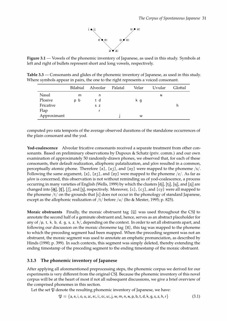
The Corpus of Spontaneous Japanese 31
i • i:
e • e:
a • a:
o • o:
u • u:
Figure 3.1—Vowels of the phonemic inventory of Japanese, as used in this study. Symbols atleft and right of bullets represent short and long vowels, respectively.
Table 3.3— Consonants and glides of the phonemic inventory of Japanese, as used in this study.Where symbols appear in pairs, the one to the right represents a voiced consonant.
Bilabial Alveolar Palatal Velar Uvular Glottal
Nasal m n ðPlosive p b t d k gFricative s z hFlap rApproximant j w
computed pro rata temporis of the average observed durations of the standalone occurrences ofthe plain consonant and the yod.
Yod-coalescence Alveolar fricative consonants received a separate treatment from other con-sonants. Based on preliminary observations by Dupoux & Schatz (priv. comm.) and our ownexamination of approximately 50 randomly-drawn phones, we observed that, for each of theseconsonants, their default realization, allophonic palatalization, and yoon resulted in a common,perceptually atomic phone. Therefore [s], [sj], and [sy] were mapped to the phoneme /s/.Following the same argument, [z], [zj], and [zy] were mapped to the phoneme /z/. As far asyoon is concerned, this observation is not without reminding us of yod-coalescence, a processoccurring in many varieties of English (Wells, 1999) by which the clusters [dj], [tj], [sj], and [zj] arechanged into [Ã], [Ù], [S], and [Z], respectively. Moreover, [c], [cj], and [cy]were all mapped tothe phoneme /t/ on the grounds that [c] does not occur in the phonology of standard Japanese,except as the allophonic realization of /t/ before /u/ (Ito & Mester, 1995; p. 825).
Moraic obstruents Finally, the moraic obstruent tag [Q] was used throughout the CSJ toannotate the second half of a geminate obstruent and, hence, serves as an abstract placeholder forany of /p, t, k, b, d, g, s, z, h/, depending on the context. In order to set all obstruents apart, andfollowing our discussion on the moraic chroneme tag [H], this tag was mapped to the phonemeto which the preceding segment had been mapped. When the preceding segment was not anobstruent, the moraic segment was used to annotate an emphatic pronunciation, as described byHinds (1990; p. 399). In such contexts, this segment was simply deleted, thereby extending theending timestamp of the preceding segment to the ending timestamp of the moraic obstruent.
3.1.3 The phonemic inventory of Japanese
After applying all aforementioned preprocessing steps, the phonemic corpus we derived for ourexperiments is very different from the original CSJ. Because the phonemic inventory of this novelcorpus will be at the heart of most if not all subsequent discussions, we give a brief overview ofthe comprised phonemes in this section.Let the set P denote the resulting phonemic inventory of Japanese, we have:
P ≡ a, e, i, o, u, a:, e:, i:, o:, u:, j, w, m, n, ð, p, b, t, d, k, g, s, z, h, r (3.1)
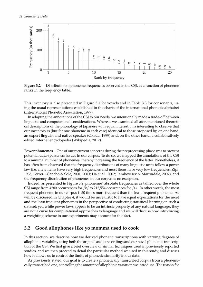
32 Sources of Data
1 5 10 15 20 250
100
200a
oi t
e ku s n
r m ð d o: g je: h z w u: b a: p i:
Rank by frequency
Freq
uenc
y(in
thou
sand
s)
Figure 3.2—Distribution of phoneme frequencies observed in the CSJ, as a function of phonemeranks in the frequency table.
This inventory is also presented in Figure 3.1 for vowels and in Table 3.3 for consonants, us-ing the usual representations established in the charts of the international phonetic alphabet(International Phonetic Association, 1999).
In adapting the annotations of the CSJ to our needs, we intentionally made a trade-off betweenlinguistic and computational considerations. Whereas we examined all aforementioned theoreti-cal descriptions of the phonology of Japanese with equal interest, it is interesting to observe thatour inventory is (but for one phoneme in each case) identical to those proposed by, on one hand,an expert linguist and native speaker (Okada, 1999) and, on the other hand, a collaborativelyedited Internet encyclopedia (Wikipedia, 2012).
Power phonemes One of our recurrent concerns during the preprocessing phasewas to preventpotential data-sparseness issues in our corpus. To do so, we mapped the annotations of the CSJto a minimal number of phonemes, thereby increasing the frequency of the latter. Nonetheless, ithas often been observed that the frequency distributions of many linguistic units follow a powerlaw (i.e. a few items have very high frequencies and most items have very low frequencies; Zipf,1935; Ferrer-i-Cancho & Solé, 2001, 2003; Ha et al., 2002; Tambovtsev & Martindale, 2007), andthe frequency distribution of phonemes in our corpus is no exception.Indeed, as presented in Figure 3.2, phonemes’ absolute frequencies as tallied over the whole
CSJ range from 4280 occurrences for /i:/ to 212,554 occurrences for /a/. In other words, the mostfrequent phoneme in our corpus is 50 times more frequent than the least frequent phoneme. Aswill be discussed in Chapter 4, it would be unrealistic to have equal expectations for the mostand the least frequent phonemes in the perspective of conducting statistical learning on such adataset; yet, while power laws appear to be an intrinsic property of any natural language, theyare not a curse for computational approaches to language and we will discuss how introducinga weighting scheme in our experiments may account for this fact.
3.2 Good allophones like yo momma used to cook
In this section, we describe how we derived phonetic transcriptions with varying degrees ofallophonic variability using both the original audio recordings and our novel phonemic transcrip-tion of the CSJ. We first give a brief overview of similar techniques used in previously reportedstudies, and we then proceed to detail the particular method we used in this study, and discusshow it allows us to control the limits of phonetic similarity in our data.As previously stated, our goal is to create a phonetically transcribed corpus from a phonemi-
cally transcribed one, controlling the amount of allophonic variationwe introduce. The reason for
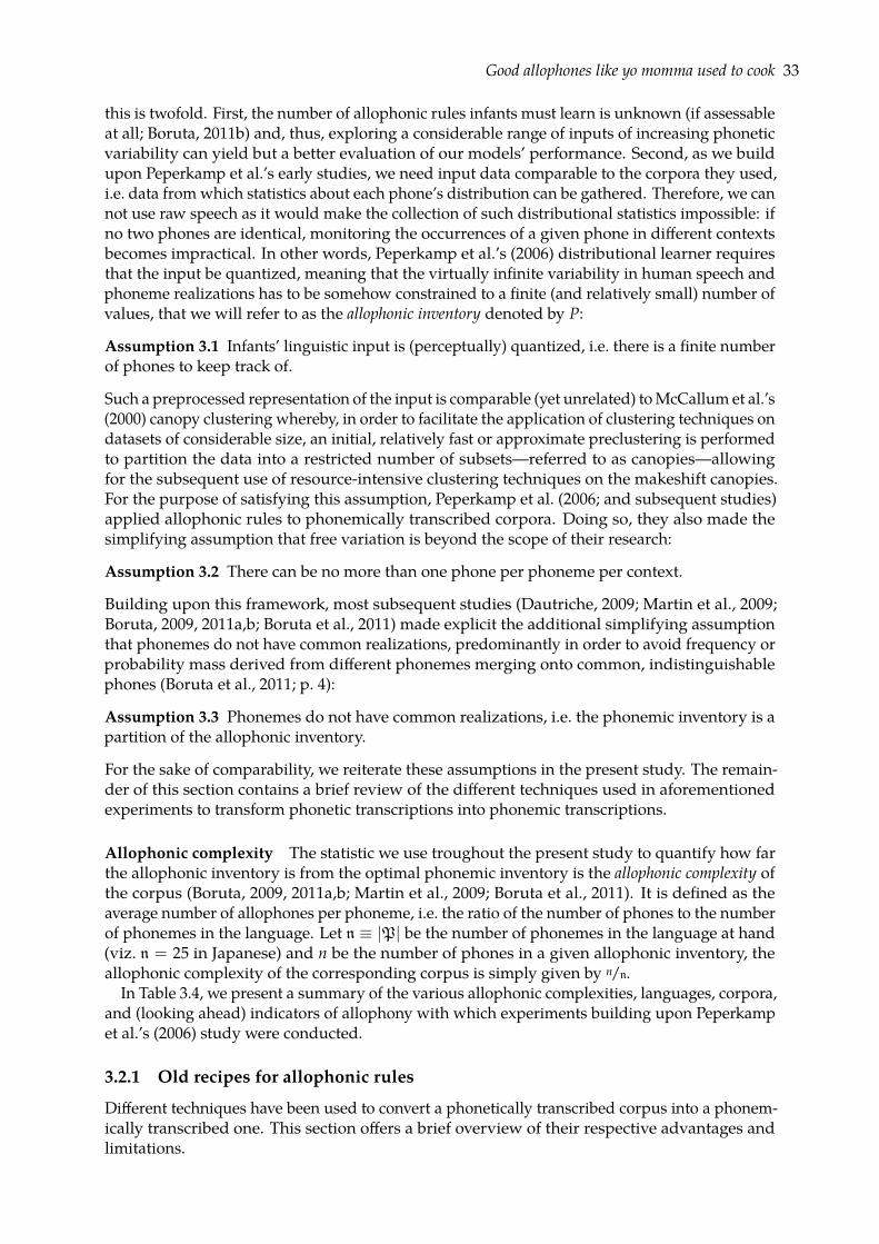
Good allophones like yo momma used to cook 33
this is twofold. First, the number of allophonic rules infants must learn is unknown (if assessableat all; Boruta, 2011b) and, thus, exploring a considerable range of inputs of increasing phoneticvariability can yield but a better evaluation of our models’ performance. Second, as we buildupon Peperkamp et al.’s early studies, we need input data comparable to the corpora they used,i.e. data from which statistics about each phone’s distribution can be gathered. Therefore, we cannot use raw speech as it would make the collection of such distributional statistics impossible: ifno two phones are identical, monitoring the occurrences of a given phone in different contextsbecomes impractical. In other words, Peperkamp et al.’s (2006) distributional learner requiresthat the input be quantized, meaning that the virtually infinite variability in human speech andphoneme realizations has to be somehow constrained to a finite (and relatively small) number ofvalues, that we will refer to as the allophonic inventory denoted by P:
Assumption 3.1 Infants’ linguistic input is (perceptually) quantized, i.e. there is a finite numberof phones to keep track of.
Such a preprocessed representation of the input is comparable (yet unrelated) toMcCallum et al.’s(2000) canopy clustering whereby, in order to facilitate the application of clustering techniques ondatasets of considerable size, an initial, relatively fast or approximate preclustering is performedto partition the data into a restricted number of subsets—referred to as canopies—allowingfor the subsequent use of resource-intensive clustering techniques on the makeshift canopies.For the purpose of satisfying this assumption, Peperkamp et al. (2006; and subsequent studies)applied allophonic rules to phonemically transcribed corpora. Doing so, they also made thesimplifying assumption that free variation is beyond the scope of their research:
Assumption 3.2 There can be no more than one phone per phoneme per context.
Building upon this framework, most subsequent studies (Dautriche, 2009; Martin et al., 2009;Boruta, 2009, 2011a,b; Boruta et al., 2011) made explicit the additional simplifying assumptionthat phonemes do not have common realizations, predominantly in order to avoid frequency orprobability mass derived from different phonemes merging onto common, indistinguishablephones (Boruta et al., 2011; p. 4):
Assumption 3.3 Phonemes do not have common realizations, i.e. the phonemic inventory is apartition of the allophonic inventory.
For the sake of comparability, we reiterate these assumptions in the present study. The remain-der of this section contains a brief review of the different techniques used in aforementionedexperiments to transform phonetic transcriptions into phonemic transcriptions.
Allophonic complexity The statistic we use troughout the present study to quantify how farthe allophonic inventory is from the optimal phonemic inventory is the allophonic complexity ofthe corpus (Boruta, 2009, 2011a,b; Martin et al., 2009; Boruta et al., 2011). It is defined as theaverage number of allophones per phoneme, i.e. the ratio of the number of phones to the numberof phonemes in the language. Let n ≡ |P| be the number of phonemes in the language at hand(viz. n = 25 in Japanese) and n be the number of phones in a given allophonic inventory, theallophonic complexity of the corresponding corpus is simply given by n/n.
In Table 3.4, we present a summary of the various allophonic complexities, languages, corpora,and (looking ahead) indicators of allophony with which experiments building upon Peperkampet al.’s (2006) study were conducted.
3.2.1 Old recipes for allophonic rules
Different techniques have been used to convert a phonetically transcribed corpus into a phonem-ically transcribed one. This section offers a brief overview of their respective advantages andlimitations.
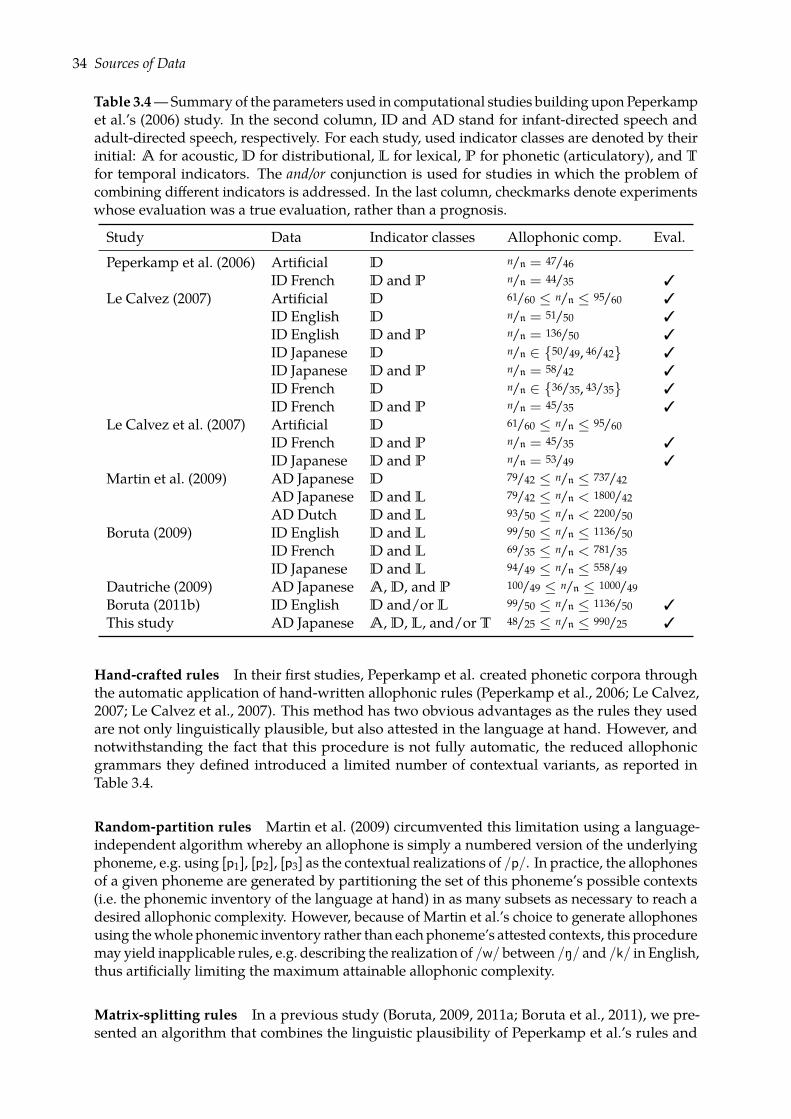
34 Sources of Data
Table 3.4—Summary of the parameters used in computational studies building upon Peperkampet al.’s (2006) study. In the second column, ID and AD stand for infant-directed speech andadult-directed speech, respectively. For each study, used indicator classes are denoted by theirinitial: A for acoustic, D for distributional, L for lexical, P for phonetic (articulatory), and T
for temporal indicators. The and/or conjunction is used for studies in which the problem ofcombining different indicators is addressed. In the last column, checkmarks denote experimentswhose evaluation was a true evaluation, rather than a prognosis.
Study Data Indicator classes Allophonic comp. Eval.
Peperkamp et al. (2006) Artificial D n/n = 47/46
ID French D and P n/n = 44/35 3
Le Calvez (2007) Artificial D 61/60 ≤ n/n ≤ 95/60 3
ID English D n/n = 51/50 3
ID English D and P n/n = 136/50 3
ID Japanese D n/n ∈ 50/49, 46/42 3
ID Japanese D and P n/n = 58/42 3
ID French D n/n ∈ 36/35, 43/35 3
ID French D and P n/n = 45/35 3
Le Calvez et al. (2007) Artificial D 61/60 ≤ n/n ≤ 95/60
ID French D and P n/n = 45/35 3
ID Japanese D and P n/n = 53/49 3
Martin et al. (2009) AD Japanese D 79/42 ≤ n/n ≤ 737/42
AD Japanese D and L 79/42 ≤ n/n < 1800/42
AD Dutch D and L 93/50 ≤ n/n < 2200/50
Boruta (2009) ID English D and L 99/50 ≤ n/n ≤ 1136/50
ID French D and L 69/35 ≤ n/n < 781/35
ID Japanese D and L 94/49 ≤ n/n ≤ 558/49
Dautriche (2009) AD Japanese A, D, and P 100/49 ≤ n/n ≤ 1000/49
Boruta (2011b) ID English D and/or L 99/50 ≤ n/n ≤ 1136/50 3
This study AD Japanese A, D, L, and/or T 48/25 ≤ n/n ≤ 990/25 3
Hand-crafted rules In their first studies, Peperkamp et al. created phonetic corpora throughthe automatic application of hand-written allophonic rules (Peperkamp et al., 2006; Le Calvez,2007; Le Calvez et al., 2007). This method has two obvious advantages as the rules they usedare not only linguistically plausible, but also attested in the language at hand. However, andnotwithstanding the fact that this procedure is not fully automatic, the reduced allophonicgrammars they defined introduced a limited number of contextual variants, as reported inTable 3.4.
Random-partition rules Martin et al. (2009) circumvented this limitation using a language-independent algorithm whereby an allophone is simply a numbered version of the underlyingphoneme, e.g. using [p1], [p2], [p3] as the contextual realizations of /p/. In practice, the allophonesof a given phoneme are generated by partitioning the set of this phoneme’s possible contexts(i.e. the phonemic inventory of the language at hand) in as many subsets as necessary to reach adesired allophonic complexity. However, because of Martin et al.’s choice to generate allophonesusing thewhole phonemic inventory rather than each phoneme’s attested contexts, this proceduremay yield inapplicable rules, e.g. describing the realization of /w/ between /N/ and /k/ in English,thus artificially limiting the maximum attainable allophonic complexity.
Matrix-splitting rules In a previous study (Boruta, 2009, 2011a; Boruta et al., 2011), we pre-sented an algorithm that combines the linguistic plausibility of Peperkamp et al.’s rules and
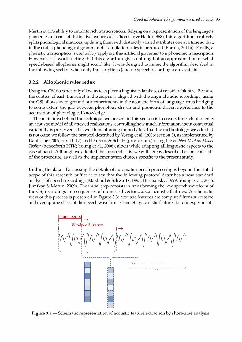
Good allophones like yo momma used to cook 35
Martin et al.’s ability to emulate rich transcriptions. Relying on a representation of the language’sphonemes in terms of distinctive features à la Chomsky & Halle (1968), this algorithm iterativelysplits phonological matrices, updating themwith distinctly valued attributes one at a time so that,in the end, a phonological grammar of assimilation rules is produced (Boruta, 2011a). Finally, aphonetic transcription is created by applying this artificial grammar to a phonemic transcription.However, it is worth noting that this algorithm gives nothing but an approximation of whatspeech-based allophones might sound like. It was designed to mimic the algorithm described inthe following section when only transcriptions (and no speech recordings) are available.
3.2.2 Allophonic rules redux
Using the CSJ does not only allow us to explore a linguistic database of considerable size. Becausethe content of each transcript in the corpus is aligned with the original audio recordings, usingthe CSJ allows us to ground our experiments in the acoustic form of language, thus bridgingto some extent the gap between phonology-driven and phonetics-driven approaches to theacquisition of phonological knowledge.
The main idea behind the technique we present in this section is to create, for each phoneme,an acoustic model of all attested realizations, controlling howmuch information about contextualvariability is preserved. It is worth mentioning immediately that the methodology we adoptedis not ours: we follow the protocol described by Young et al. (2006; section 3), as implemented byDautriche (2009; pp. 11–17) and Dupoux & Schatz (priv. comm.) using the Hidden Markov ModelToolkit (henceforth HTK; Young et al., 2006), albeit while adapting all linguistic aspects to thecase at hand. Although we adopted this protocol as-is, we will hereby describe the core conceptsof the procedure, as well as the implementation choices specific to the present study.
Coding the data Discussing the details of automatic speech processing is beyond the statedscope of this research; suffice it to say that the following protocol describes a now-standardanalysis of speech recordings (Makhoul & Schwartz, 1995; Hermansky, 1999; Young et al., 2006;Jurafksy & Martin, 2009). The initial step consists in transforming the raw speech waveform ofthe CSJ recordings into sequences of numerical vectors, a.k.a. acoustic features. A schematicview of this process is presented in Figure 3.3: acoustic features are computed from successiveand overlapping slices of the speech waveform. Concretely, acoustic features for our experiments
Frame period →Window duration →
Figure 3.3— Schematic representation of acoustic feature extraction by short-time analysis.
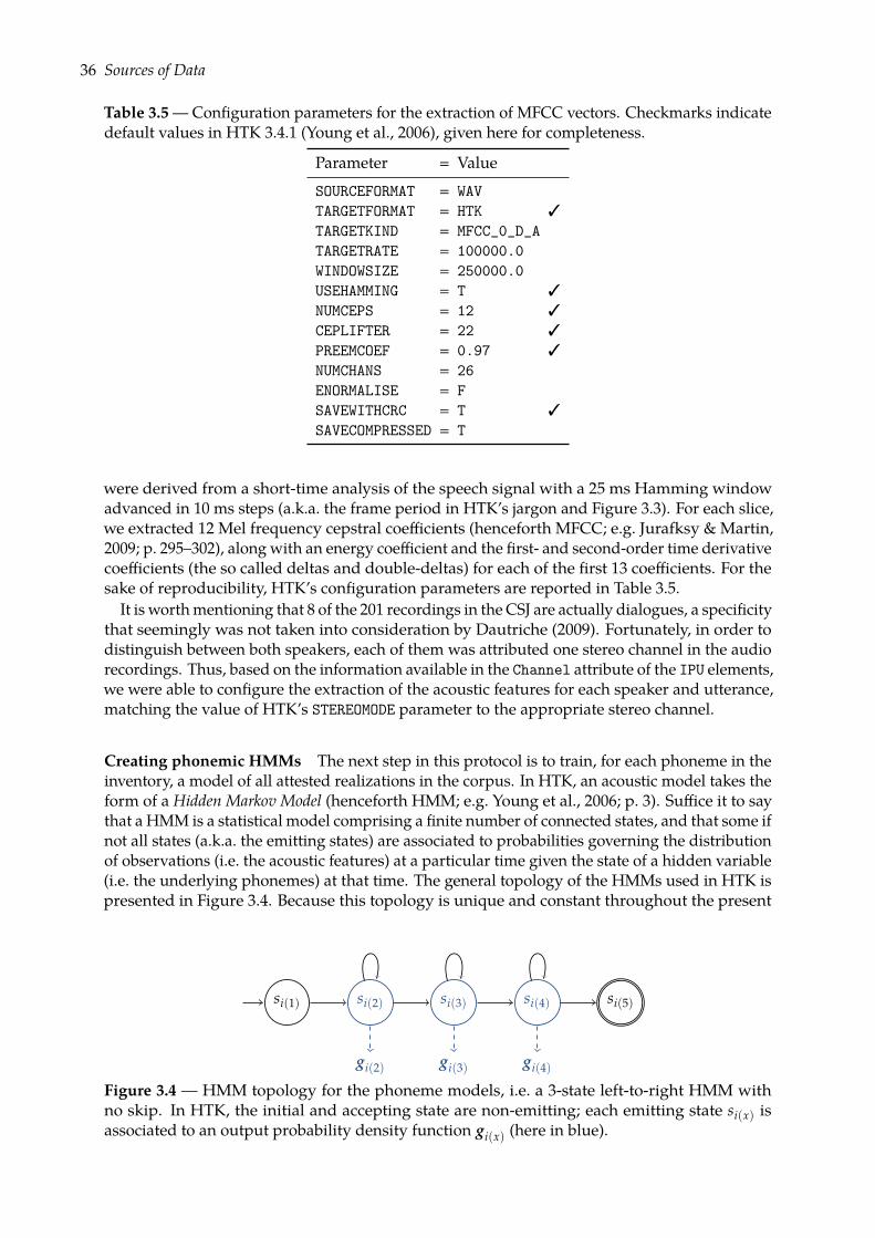
36 Sources of Data
Table 3.5 — Configuration parameters for the extraction of MFCC vectors. Checkmarks indicatedefault values in HTK 3.4.1 (Young et al., 2006), given here for completeness.
Parameter = Value
SOURCEFORMAT = WAVTARGETFORMAT = HTK 3
TARGETKIND = MFCC_0_D_ATARGETRATE = 100000.0WINDOWSIZE = 250000.0USEHAMMING = T 3
NUMCEPS = 12 3
CEPLIFTER = 22 3
PREEMCOEF = 0.97 3
NUMCHANS = 26ENORMALISE = FSAVEWITHCRC = T 3
SAVECOMPRESSED = T
were derived from a short-time analysis of the speech signal with a 25 ms Hamming windowadvanced in 10 ms steps (a.k.a. the frame period in HTK’s jargon and Figure 3.3). For each slice,we extracted 12 Mel frequency cepstral coefficients (henceforth MFCC; e.g. Jurafksy & Martin,2009; p. 295–302), along with an energy coefficient and the first- and second-order time derivativecoefficients (the so called deltas and double-deltas) for each of the first 13 coefficients. For thesake of reproducibility, HTK’s configuration parameters are reported in Table 3.5.
It is worthmentioning that 8 of the 201 recordings in the CSJ are actually dialogues, a specificitythat seemingly was not taken into consideration by Dautriche (2009). Fortunately, in order todistinguish between both speakers, each of them was attributed one stereo channel in the audiorecordings. Thus, based on the information available in the Channel attribute of the IPU elements,we were able to configure the extraction of the acoustic features for each speaker and utterance,matching the value of HTK’s STEREOMODE parameter to the appropriate stereo channel.
Creating phonemic HMMs The next step in this protocol is to train, for each phoneme in theinventory, a model of all attested realizations in the corpus. In HTK, an acoustic model takes theform of a Hidden Markov Model (henceforth HMM; e.g. Young et al., 2006; p. 3). Suffice it to saythat a HMM is a statistical model comprising a finite number of connected states, and that some ifnot all states (a.k.a. the emitting states) are associated to probabilities governing the distributionof observations (i.e. the acoustic features) at a particular time given the state of a hidden variable(i.e. the underlying phonemes) at that time. The general topology of the HMMs used in HTK ispresented in Figure 3.4. Because this topology is unique and constant throughout the present
si(1) si(2) si(3) si(4) si(5)
gi(2) gi(3) gi(4)
Figure 3.4 — HMM topology for the phoneme models, i.e. a 3-state left-to-right HMM withno skip. In HTK, the initial and accepting state are non-emitting; each emitting state si(x) isassociated to an output probability density function gi(x) (here in blue).
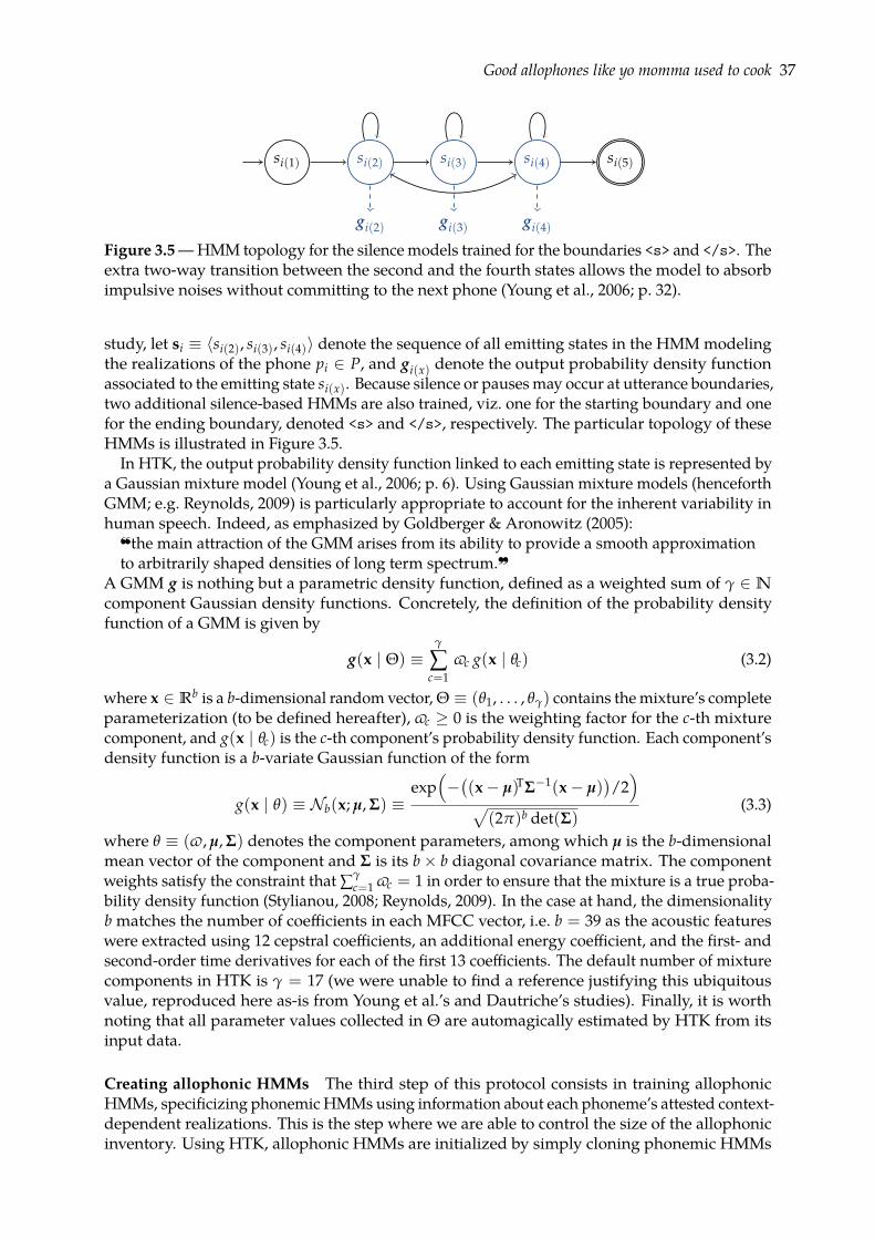
Good allophones like yo momma used to cook 37
si(1) si(2) si(3) si(4) si(5)
gi(2) gi(3) gi(4)
Figure 3.5—HMM topology for the silence models trained for the boundaries <s> and </s>. Theextra two-way transition between the second and the fourth states allows the model to absorbimpulsive noises without committing to the next phone (Young et al., 2006; p. 32).
study, let si ≡ 〈si(2), si(3), si(4)〉 denote the sequence of all emitting states in the HMM modelingthe realizations of the phone pi ∈ P, and gi(x) denote the output probability density functionassociated to the emitting state si(x). Because silence or pauses may occur at utterance boundaries,two additional silence-based HMMs are also trained, viz. one for the starting boundary and onefor the ending boundary, denoted <s> and </s>, respectively. The particular topology of theseHMMs is illustrated in Figure 3.5.
In HTK, the output probability density function linked to each emitting state is represented bya Gaussian mixture model (Young et al., 2006; p. 6). Using Gaussian mixture models (henceforthGMM; e.g. Reynolds, 2009) is particularly appropriate to account for the inherent variability inhuman speech. Indeed, as emphasized by Goldberger & Aronowitz (2005):
the main attraction of the GMM arises from its ability to provide a smooth approximationto arbitrarily shaped densities of long term spectrum.~
A GMM g is nothing but a parametric density function, defined as a weighted sum of γ ∈ N
component Gaussian density functions. Concretely, the definition of the probability densityfunction of a GMM is given by
g(x | Θ) ≡γ
∑c=1
vc g(x | θc) (3.2)
where x ∈ Rb is a b-dimensional random vector, Θ ≡ (θ1, . . . , θγ) contains themixture’s completeparameterization (to be defined hereafter), vc ≥ 0 is the weighting factor for the c-th mixturecomponent, and g(x | θc) is the c-th component’s probability density function. Each component’sdensity function is a b-variate Gaussian function of the form
g(x | θ) ≡ Nb(x; µ, Σ) ≡exp
(−((x− µ)TΣ−1(x− µ)
)/2)
√(2π)b det(Σ)
(3.3)
where θ ≡ (v, µ, Σ) denotes the component parameters, among which µ is the b-dimensionalmean vector of the component and Σ is its b× b diagonal covariance matrix. The componentweights satisfy the constraint that ∑γ
c=1 vc = 1 in order to ensure that the mixture is a true proba-bility density function (Stylianou, 2008; Reynolds, 2009). In the case at hand, the dimensionalityb matches the number of coefficients in each MFCC vector, i.e. b = 39 as the acoustic featureswere extracted using 12 cepstral coefficients, an additional energy coefficient, and the first- andsecond-order time derivatives for each of the first 13 coefficients. The default number of mixturecomponents in HTK is γ = 17 (we were unable to find a reference justifying this ubiquitousvalue, reproduced here as-is from Young et al.’s and Dautriche’s studies). Finally, it is worthnoting that all parameter values collected in Θ are automagically estimated by HTK from itsinput data.
Creating allophonic HMMs The third step of this protocol consists in training allophonicHMMs, specificizing phonemic HMMs using information about each phoneme’s attested context-dependent realizations. This is the step where we are able to control the size of the allophonicinventory. Using HTK, allophonic HMMs are initialized by simply cloning phonemic HMMs
38 Sources of Data
and then retraining all models using so called triphone transcriptions (Young et al., 2006; p. 34–36), i.e. phonetic transcriptions where each phone is denoted by the trigram made up of thepreceding phoneme, the target phoneme, and the following phoneme. For example, using HTK’sminus-plus notation and visible spaces to denote segment boundaries, an utterance consisting ofthe word /sake/, would be transcribed as <s>-s+as-a+ka-k+ek-e+</s>where s-a+k denotesthe realization of the phoneme /a/ between /s/ and /k/—the treatment of the initial and finalsegments was simplified for the sake of the example. It is worth noting that such a transcriptionyields the highest attainable allophonic complexity for any corpus. Indeed, following Peperkampet al. (2006; and subsequent studies), we assumed that there can be no more than one phone perphoneme per context (Assumption 3.2). In a triphone transcription, a phone is systematicallyrepresented by the trigrammade up of the underlying phoneme and its attested context. Overall,the allophonic inventory in such a transcription comprises, for every phoneme in the languageat hand, the set of all realizations in all attested contexts. Therefore, we can not further increasethe allophonic complexity of our dataset while still satisfying the aforementioned assumption.Having re-estimated the parameters of all allophonic HMMs, the next step consists in con-
trolling the overall allophonic complexity by merging, for each phoneme, some of these utterlyspecified allophones—a procedure known as state-tying in HTK’s jargon (Young et al., 2006;pp. 36–39, 144–146). For a given phoneme and a given emitting state position x ∈ 2, 3, 4,the x-th states of all allophonic HMMs of this phoneme are first pooled into a single cluster,and then iteratively partitioned into an arborescent structure resembling a decision tree; thisprocess is repeated for each phoneme and each of the three emitting states in the HMMs. Theiterative partitioning relies on a set of a priori linguistic questions ranging from natural classes(e.g. consonants, vowels, stops) to specific contexts; the questions we designed for the purposeof the present study are reported in Table 3.6 where each set of contexts was used to createquestions for both preceding and following contexts. For a given cluster, HTK applies eachquestion in turn, tentatively splitting the cluster into two new branches comprising, on one hand,phones whose realization context belongs the question’s application contexts (e.g. the phone’scontext is a voiced phoneme) and, on the other hand, phones whose realization context does notbelong to the question (e.g. the phone’s context is not a voiced phoneme). The question whichmaximizes the likelihood of the data—i.e. the probability of partitioning these given phones inthis particular way given the training data—is then effectively used to split the initial cluster, andthis process is repeated on every new branch until an a priori global threshold (to be discussedhereafter) is reached. In the end, for each leaf in this newly created decision tree, the HMMstates within that leaf are said to be tied in the sense that, during a final re-estimation of allmodels’ parameters, a single, common GMM is used for every set of tied states. The number ofallophones that were computed for a given phoneme is defined as the sum, for each emittingstate, of the number of distinct (i.e. not tied) leaves.Once all state-tying has been completed, some allophones may share the exact same HMM
and, in that case, the corresponding phones are indistinguishable (at least in our quantizedrepresentation). Following the work of Dautriche (2009) and Dupoux & Schatz (priv. comm.), ourtermination criterion for state-tying relies on the global number of such tied, indistinguishablephones: let n denote the desired number of phones in the allophonic inventory, our solutionconsists in the inventory that maximizes the overall likelihood of the tied allophonic HMMs giventhe CSJ, and whose size n is as close as possible to n. Indeed, because of unspecified reasons,Dautriche’s and Dupoux & Schatz’s programs, though determinist, do not always output aninventory comprising the exact desired number of phones; observed differences between thedesired and the actual number of phones range from −18 to +2.
As previously stated, our goal is to explore a considerable range of inputs of increasing phoneticvariability. In order to do so, we ran 20 distinct state-tying procedures controlling the a priorisize of the allophonic inventory, ranging from 50 phones to 1000 phones in increments of 50.Whereas the lower bound and the increment were chosen arbitrarily, it should be noted thatrequesting allophonic complexities higher than 1000/25 requires considerable computing time
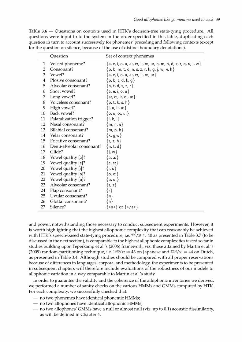
Good allophones like yo momma used to cook 39
Table 3.6 — Questions on contexts used in HTK’s decision-tree state-tying procedure. Allquestions were input to to the system in the order specified in this table, duplicating eachquestion in turn to account successively for phonemes’ preceding and following contexts (exceptfor the question on silence, because of the use of distinct boundary denotations).
Question Set of context phonemes
1 Voiced phoneme? a, e, i, o, u, a:, e:, i:, o:, u:, b, m, n, d, z, r, g, ð, j, w2 Consonant? p, b, m, t, d, n, s, z, r, k, g, j, w, ð, h3 Vowel? a, e, i, o, u, a:, e:, i:, o:, u:4 Plosive consonant? p, b, t, d, k, g5 Alveolar consonant? n, t, d, s, z, r6 Short vowel? a, e, i, o, u7 Long vowel? a:, e:, i:, o:, u:8 Voiceless consonant? p, t, k, s, h9 High vowel? i, u, i:, u:10 Back vowel? o, u, o:, u:11 Palatalization trigger? i, i:, j12 Nasal consonant? m, n, ð13 Bilabial consonant? m, p, b14 Velar consonant? k, g,w15 Fricative consonant? s, z, h16 Denti-alveolar consonant? n, t, d17 Glide? j, w18 Vowel quality [a]? a, a:19 Vowel quality [e]? e, e:20 Vowel quality [i]? i, i:21 Vowel quality [o]? o, o:22 Vowel quality [u]? u, u:23 Alveolar consonant? s, z24 Flap consonant? r25 Uvular consonant? ð26 Glottal consonant? h27 Silence? <s> or </s>
and power, notwithstanding those necessary to conduct subsequent experiments. However, itis worth highlighting that the highest allophonic complexity that can reasonably be achievedwith HTK’s speech-based state-tying procedure, i.e. 990/25 ≈ 40 as presented in Table 3.7 (to bediscussed in the next section), is comparable to the highest allophonic complexities tested so far instudies building upon Peperkamp et al.’s (2006) framework, viz. those attained by Martin et al.’s(2009) random-partitioning technique, i.e. 1800/42 ≈ 43 on Japanese and 2200/50 = 44 on Dutch,as presented in Table 3.4. Although studies should be compared with all proper reservationsbecause of differences in languages, corpora, and methodology, the experiments to be presentedin subsequent chapters will therefore include evaluations of the robustness of our models toallophonic variation in a way comparable to Martin et al.’s study.
In order to guarantee the validity and the coherence of the allophonic inventories we derived,we performed a number of sanity checks on the various HMMs and GMMs computed by HTK.For each complexity, we successfully checked that:— no two phonemes have identical phonemic HMMs;— no two allophones have identical allophonic HMMs;— no two allophones’ GMMs have a null or almost null (viz. up to 0.1) acoustic dissimilarity,
as will be defined in Chapter 4.
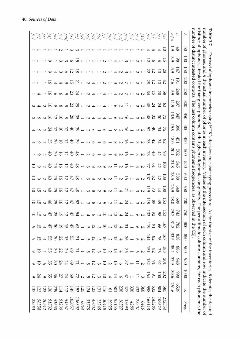
40 Sources of Data
Table3.7
—Derived
allophonicinventoriesusing
HTK
’sdecision-treestate-tying
procedure.Asforthe
sizeofthe
inventories,ndenotesthe
desirednum
berofphones,andnthe
actualnumberofphonesin
eachinventory.Valuesatthe
intersectionofeach
columnand
rowindicate
thenum
berofdistinctallophonesattested
forthatgivenphonem
eatthatgiven
allophoniccom
plexity.Thepenultim
atecolum
ncontains,foreach
phoneme,the
numberofdistinctattested
contexts.Thelastcolum
ncontainsphonem
efrequencies,asobserved
inthe
CSJ.
n50
100150
200250
300350
400450
500550
600650
700750
800850
900950
1000∞
Freq.
n48
98147
191248
297347
398451
502545
588648
699743
782838
886948
9906539
n/n
1.93.9
5.97.6
9.911.9
13.915.9
18.020.1
21.823.5
25.928.0
29.731.3
33.535.4
37.939.6
261.6
/a/10
1528
4258
6372
7282
98103
108130
153153
167167
183201
202585
212554/e/
46
1010
2024
3034
3442
4242
4449
5866
7676
92100
504109624
/i/4
612
1215
2432
4042
4861
6273
8992
9182
8291
91532
143285/o/
412
2228
3448
4852
7373
77107
119119
132119
144151
152164
598165113
/a:/1
11
12
22
22
22
22
22
22
22
3368
6416/e:/
12
22
22
22
33
33
33
66
66
1111
43223207
/i:/1
11
11
11
11
11
11
11
11
11
1338
4280/o:/
13
37
711
1616
1616
1616
2124
2431
3636
3737
47737693
/u:/1
12
22
22
22
22
24
44
44
46
6238
16527/u/
14
43
46
68
89
1111
1111
1313
1313
1514
50193155
/w/
11
11
11
11
11
22
22
22
22
24
6119925
/j/1
22
24
44
66
69
99
910
1010
1010
10116
30418/b/
11
11
11
11
11
22
22
23
33
33
13113248
/d/1
11
44
44
66
68
88
88
1212
1212
12123
47002/g/
11
12
22
22
22
33
33
45
55
55
12431778
/p/1
11
11
11
11
11
11
11
11
11
2125
6064/t/
315
1821
2429
3539
3948
4848
4852
5463
7171
7172
153136392
/k/3
612
1523
2328
4040
4040
4747
4747
4753
6969
69149
105057/m
/1
36
99
99
1212
1212
1212
1212
1515
2024
24112
54567/n/
23
34
68
1010
1016
1616
1616
1919
2222
2427
11491230
/ð/1
14
46
812
1220
2025
2525
2525
3030
3030
36239
51650/s/
19
916
1616
1624
3540
4040
4040
4747
5555
5555
13691532
/z/1
11
11
22
22
22
22
22
44
46
9123
20512/r/
11
11
44
99
99
99
1515
1515
1519
1924
12358354
/h/1
11
11
22
44
410
1010
1010
99
99
9137
22383
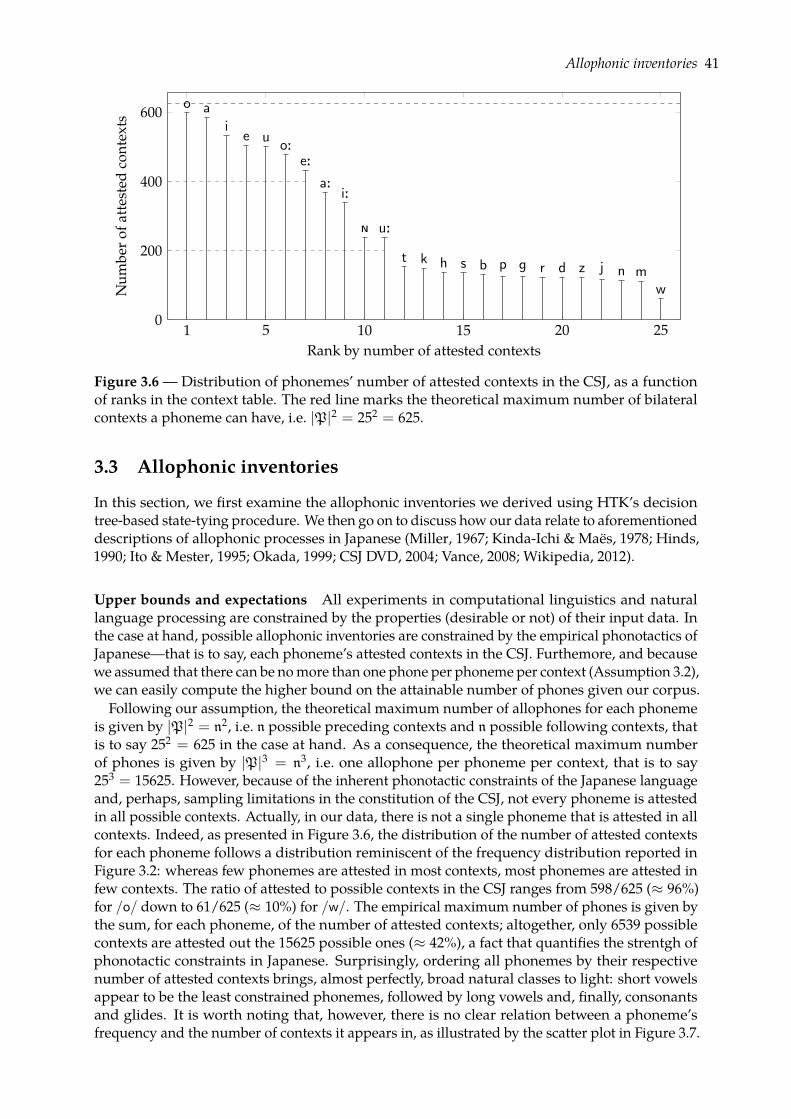
Allophonic inventories 41
1 5 10 15 20 250
200
400
600o a
ie u
o:e:
a:i:
ð u:
t k h s b p g r d z j n mw
Rank by number of attested contexts
Num
bero
fatte
sted
cont
exts
Figure 3.6 — Distribution of phonemes’ number of attested contexts in the CSJ, as a functionof ranks in the context table. The red line marks the theoretical maximum number of bilateralcontexts a phoneme can have, i.e. |P|2 = 252 = 625.
3.3 Allophonic inventories
In this section, we first examine the allophonic inventories we derived using HTK’s decisiontree-based state-tying procedure. We then go on to discuss how our data relate to aforementioneddescriptions of allophonic processes in Japanese (Miller, 1967; Kinda-Ichi & Maës, 1978; Hinds,1990; Ito & Mester, 1995; Okada, 1999; CSJ DVD, 2004; Vance, 2008; Wikipedia, 2012).
Upper bounds and expectations All experiments in computational linguistics and naturallanguage processing are constrained by the properties (desirable or not) of their input data. Inthe case at hand, possible allophonic inventories are constrained by the empirical phonotactics ofJapanese—that is to say, each phoneme’s attested contexts in the CSJ. Furthemore, and becausewe assumed that there can be nomore than one phone per phoneme per context (Assumption 3.2),we can easily compute the higher bound on the attainable number of phones given our corpus.
Following our assumption, the theoretical maximum number of allophones for each phonemeis given by |P|2 = n2, i.e. n possible preceding contexts and n possible following contexts, thatis to say 252 = 625 in the case at hand. As a consequence, the theoretical maximum numberof phones is given by |P|3 = n3, i.e. one allophone per phoneme per context, that is to say253 = 15625. However, because of the inherent phonotactic constraints of the Japanese languageand, perhaps, sampling limitations in the constitution of the CSJ, not every phoneme is attestedin all possible contexts. Actually, in our data, there is not a single phoneme that is attested in allcontexts. Indeed, as presented in Figure 3.6, the distribution of the number of attested contextsfor each phoneme follows a distribution reminiscent of the frequency distribution reported inFigure 3.2: whereas few phonemes are attested in most contexts, most phonemes are attested infew contexts. The ratio of attested to possible contexts in the CSJ ranges from 598/625 (≈ 96%)for /o/ down to 61/625 (≈ 10%) for /w/. The empirical maximum number of phones is given bythe sum, for each phoneme, of the number of attested contexts; altogether, only 6539 possiblecontexts are attested out the 15625 possible ones (≈ 42%), a fact that quantifies the strentgh ofphonotactic constraints in Japanese. Surprisingly, ordering all phonemes by their respectivenumber of attested contexts brings, almost perfectly, broad natural classes to light: short vowelsappear to be the least constrained phonemes, followed by long vowels and, finally, consonantsand glides. It is worth noting that, however, there is no clear relation between a phoneme’sfrequency and the number of contexts it appears in, as illustrated by the scatter plot in Figure 3.7.
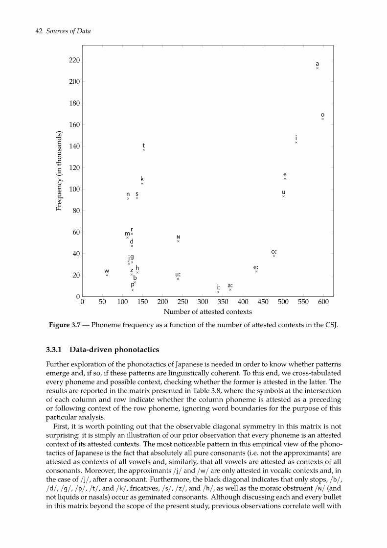
42 Sources of Data
0 50 100 150 200 250 300 350 400 450 500 550 6000
20
40
60
80
100
120
140
160
180
200
220
a:
e:
i:
o:
u:
a
e
i
o
u
w
j
b
d
g
p
t
k
m
n
ð
s
z
r
h
Number of attested contexts
Freq
uenc
y(in
thou
sand
s)
Figure 3.7 — Phoneme frequency as a function of the number of attested contexts in the CSJ.
3.3.1 Data-driven phonotactics
Further exploration of the phonotactics of Japanese is needed in order to know whether patternsemerge and, if so, if these patterns are linguistically coherent. To this end, we cross-tabulatedevery phoneme and possible context, checking whether the former is attested in the latter. Theresults are reported in the matrix presented in Table 3.8, where the symbols at the intersectionof each column and row indicate whether the column phoneme is attested as a precedingor following context of the row phoneme, ignoring word boundaries for the purpose of thisparticular analysis.
First, it is worth pointing out that the observable diagonal symmetry in this matrix is notsurprising: it is simply an illustration of our prior observation that every phoneme is an attestedcontext of its attested contexts. The most noticeable pattern in this empirical view of the phono-tactics of Japanese is the fact that absolutely all pure consonants (i.e. not the approximants) areattested as contexts of all vowels and, similarly, that all vowels are attested as contexts of allconsonants. Moreover, the approximants /j/ and /w/ are only attested in vocalic contexts and, inthe case of /j/, after a consonant. Furthermore, the black diagonal indicates that only stops, /b/,/d/, /g/, /p/, /t/, and /k/, fricatives, /s/, /z/, and /h/, as well as the moraic obstruent /ð/ (andnot liquids or nasals) occur as geminated consonants. Although discussing each and every bulletin this matrix beyond the scope of the present study, previous observations correlate well with
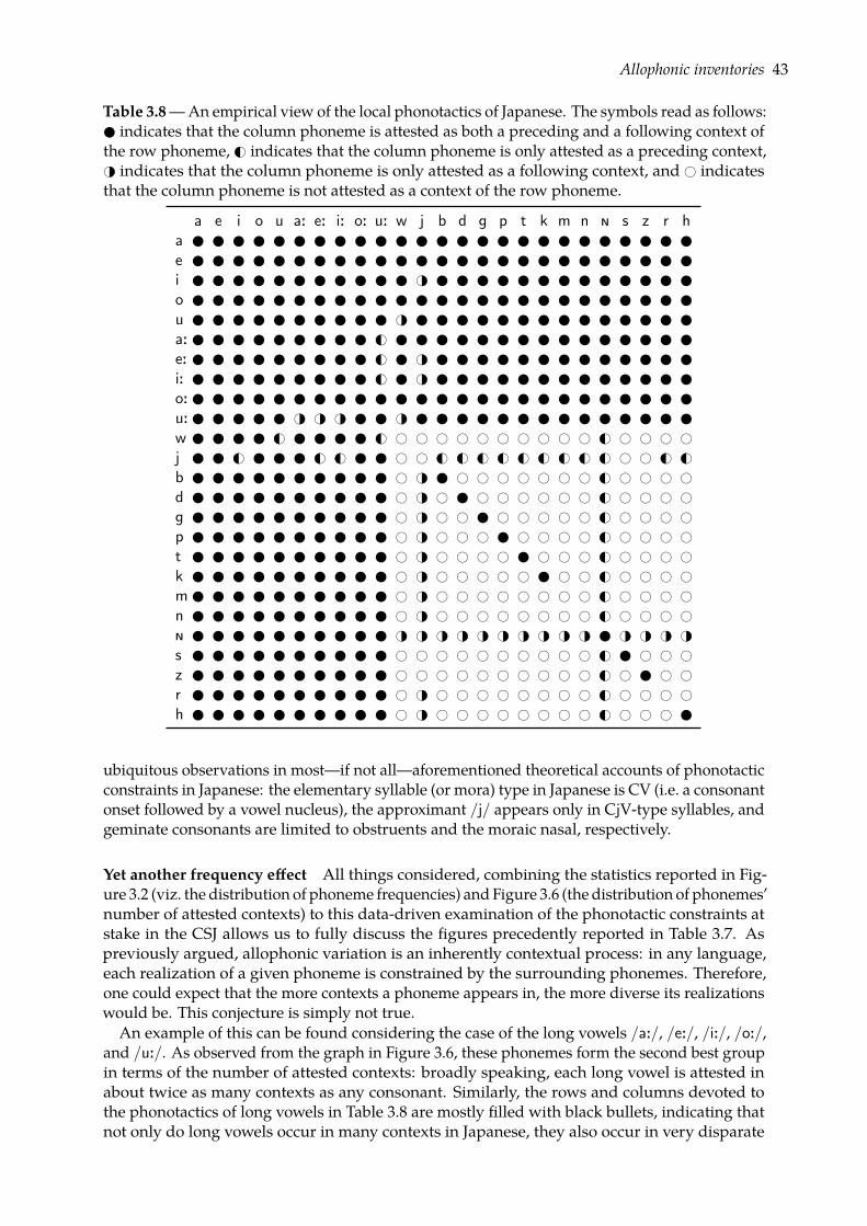
Allophonic inventories 43
Table 3.8—An empirical view of the local phonotactics of Japanese. The symbols read as follows: indicates that the column phoneme is attested as both a preceding and a following context ofthe row phoneme, G# indicates that the column phoneme is only attested as a preceding context,H# indicates that the column phoneme is only attested as a following context, and # indicatesthat the column phoneme is not attested as a context of the row phoneme.
a e i o u a: e: i: o: u: w j b d g p t k m n ð s z r ha e i H# o u H# a: G# e: G# H# i: G# H# o: u: H# H# H# H# w G# G# # # # # # # # # # # G# # # # #j G# G# G# # # G# G# G# G# G# G# G# G# G# # # G# G#b # H# # # # # # # # G# # # # #d # H# # # # # # # # G# # # # #g # H# # # # # # # # G# # # # #p # H# # # # # # # # G# # # # #t # H# # # # # # # # G# # # # #k # H# # # # # # # # G# # # # #m # H# # # # # # # # # G# # # # #n # H# # # # # # # # # G# # # # #ð H# H# H# H# H# H# H# H# H# H# H# H# H# H#s # # # # # # # # # # G# # # #z # # # # # # # # # # G# # # #r # H# # # # # # # # # G# # # # #h # H# # # # # # # # # G# # # #
ubiquitous observations in most—if not all—aforementioned theoretical accounts of phonotacticconstraints in Japanese: the elementary syllable (or mora) type in Japanese is CV (i.e. a consonantonset followed by a vowel nucleus), the approximant /j/ appears only in CjV-type syllables, andgeminate consonants are limited to obstruents and the moraic nasal, respectively.
Yet another frequency effect All things considered, combining the statistics reported in Fig-ure 3.2 (viz. the distribution of phoneme frequencies) and Figure 3.6 (the distribution of phonemes’number of attested contexts) to this data-driven examination of the phonotactic constraints atstake in the CSJ allows us to fully discuss the figures precedently reported in Table 3.7. Aspreviously argued, allophonic variation is an inherently contextual process: in any language,each realization of a given phoneme is constrained by the surrounding phonemes. Therefore,one could expect that the more contexts a phoneme appears in, the more diverse its realizationswould be. This conjecture is simply not true.
An example of this can be found considering the case of the long vowels /a:/, /e:/, /i:/, /o:/,and /u:/. As observed from the graph in Figure 3.6, these phonemes form the second best groupin terms of the number of attested contexts: broadly speaking, each long vowel is attested inabout twice as many contexts as any consonant. Similarly, the rows and columns devoted tothe phonotactics of long vowels in Table 3.8 are mostly filled with black bullets, indicating thatnot only do long vowels occur in many contexts in Japanese, they also occur in very disparate
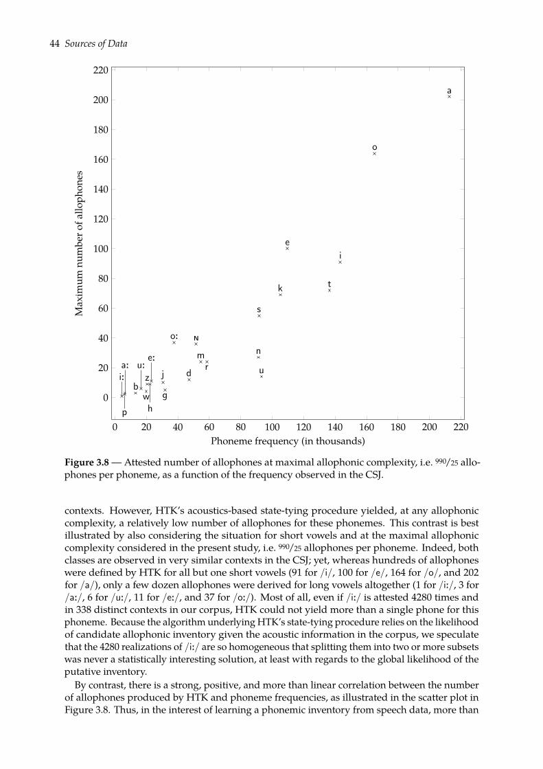
44 Sources of Data
0 20 40 60 80 100 120 140 160 180 200 220
0
20
40
60
80
100
120
140
160
180
200
220
r
gw
u:e:
h
a:
p
i:
o:
a
ei
o
u
bd
tk
m nð
s
z j
Phoneme frequency (in thousands)
Max
imum
num
bero
fallo
phon
es
Figure 3.8—Attested number of allophones at maximal allophonic complexity, i.e. 990/25 allo-phones per phoneme, as a function of the frequency observed in the CSJ.
contexts. However, HTK’s acoustics-based state-tying procedure yielded, at any allophoniccomplexity, a relatively low number of allophones for these phonemes. This contrast is bestillustrated by also considering the situation for short vowels and at the maximal allophoniccomplexity considered in the present study, i.e. 990/25 allophones per phoneme. Indeed, bothclasses are observed in very similar contexts in the CSJ; yet, whereas hundreds of allophoneswere defined by HTK for all but one short vowels (91 for /i/, 100 for /e/, 164 for /o/, and 202for /a/), only a few dozen allophones were derived for long vowels altogether (1 for /i:/, 3 for/a:/, 6 for /u:/, 11 for /e:/, and 37 for /o:/). Most of all, even if /i:/ is attested 4280 times andin 338 distinct contexts in our corpus, HTK could not yield more than a single phone for thisphoneme. Because the algorithm underlying HTK’s state-tying procedure relies on the likelihoodof candidate allophonic inventory given the acoustic information in the corpus, we speculatethat the 4280 realizations of /i:/ are so homogeneous that splitting them into two or more subsetswas never a statistically interesting solution, at least with regards to the global likelihood of theputative inventory.
By contrast, there is a strong, positive, and more than linear correlation between the numberof allophones produced by HTK and phoneme frequencies, as illustrated in the scatter plot inFigure 3.8. Thus, in the interest of learning a phonemic inventory from speech data, more than
Allophonic inventories 45
the number of attested phonemes, it appears to us that it is the frequency of a given phonemethat really dictates the variability in this phoneme’s realizations. However, further research onthis point would be needed, using other speech-processing techniques and corpora of differentsizes and languages, to be able to determine whether or not this observation is specific to ourparticular setup.
3.3.2 O theory, where art thou?
In the final section of this chapter, we attempt to compare the output of HTK’s acoustics-basedstate-tying procedure to allophonic rules presented in theoretical descriptions of allophonicprocesses in Japanese. However, it is worth immediately highlighting that a full qualitative(i.e. manual) examination of HTK’s output is hardly feasible. The reason for this is twofold.First, whereas theoretical descriptions of allophony include rules in which all elements (i.e. thetarget phoneme, the application context, and the resulting phone) are specified, e.g. h→ F / — uusing Chomsky & Halle’s (1968, p. 332) notation, HTK only instances the target phoneme andthe application contexts, the resulting allophone being represented by the HMM of its actualrealizations in the training data. Therefore, in HTK’s output, no phonetic symbol is (nor canbe) assigned to allophones, and their definition is limited to the set of all contexts in whichthey are realized. Second, and most importantly, the procedure we described in the precedingsection generates one decision tree for every phoneme, HMM emitting state, and allophoniccomplexity—that is to say 25× 3× 20 = 1500 different decision trees in the case at hand.
Established allophonic rules In Japanese, various allophonic rules constrain the realizationsof both consonants and vowels; we will review the most commonly discussed processes.As previously mentioned in this chapter, consonants are subject to a regular palatalization
process when followed by the customary palatalization triggers /i/ and /j/, e.g. s→ S / — i(Miller, 1967) and h→ ç / — i (Miller, 1967; Ito & Mester, 1995; Wikipedia, 2012). The vowel /u/,too, affects the consonants it follows by the application of allophonic rules such as h→ F / — u(Miller, 1967; Ito & Mester, 1995; Wikipedia, 2012) and t→ ţ / — u (Miller, 1967); this explainswhy, for example, the underlying form in Japanese of the English loanword tsunami is actually/tunami/. The process of lenition (a.k.a. weakening, whereby a consonant becomes more vowel-like) is also attested in Japanese for /b/ and /g/ when they occur in an intervocalic context, asexamplified by the rules b→ B / V — Vand g→ G / V — V (Kinda-Ichi&Maës, 1978;Wikipedia,2012). Finally, most if not all aforementioned sources state that the moraic nasal phoneme /ð/ issubject to strong assimilation processes: it is said to be bilabial before bilabial consonants, i.e.ð→ m / — p, b, m, coronal before coronals, i.e. ð→ n / — t, d, n, r, velar before velars, i.e.ð→ N / — k, g, and uvular [ð] in other contexts; put another way, this phoneme only carriesinformation about nasality and obstruction, its place of articulation depending on that of thefollowing phoneme.As far as vowels are concerned, the major allophonic process in Japanese is devoicing: short
vowels, and especially the high vowels /i/ and /u/, become devoiced between two voicelessconsonants (Kinda-Ichi & Maës, 1978; Wikipedia, 2012), e.g. i→ i
˚/ C
˚—C
˚and u→ u
˚/ C
˚—C
˚.
State-tying’s aftermath We now go on to examine whether these allophonic rules can be foundin HTK’s output. Before turning to the actual decision trees, the first step in our analysis concernsthe linguistic questions we provided to HTK, i.e. that we are interested in reviewing, for everyphoneme in the inventory, the questions that proved to be statistically relevant for an acoustics-based definition of its allophones. To this end, we cross-tabulated all questions and phonemes,distinguishing between questions that were actually used by HTK, questions that were not usedthough they define attested contexts for the phoneme at hand, and questions that could not beused because of phonotactic constraints on that phoneme. The results are reported in the matrixpresented in Table 3.9.
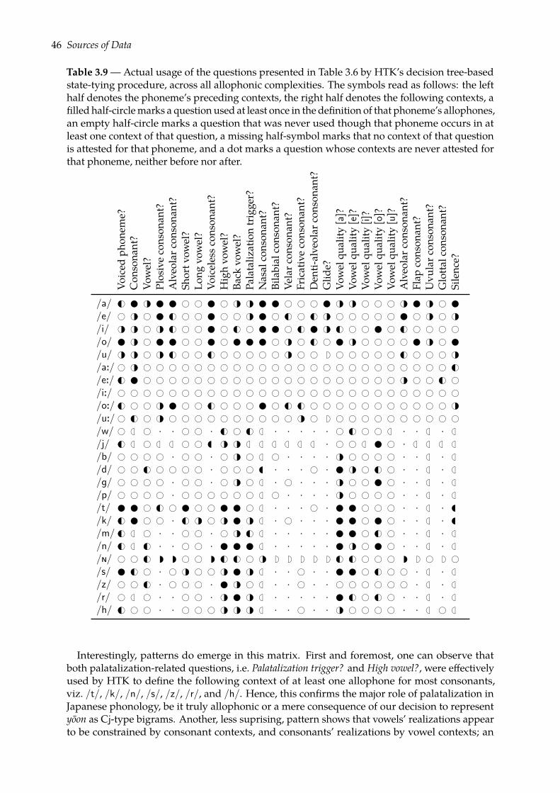
46 Sources of Data
Table 3.9—Actual usage of the questions presented in Table 3.6 by HTK’s decision tree-basedstate-tying procedure, across all allophonic complexities. The symbols read as follows: the lefthalf denotes the phoneme’s preceding contexts, the right half denotes the following contexts, afilled half-circlemarks a question used at least once in the definition of that phoneme’s allophones,an empty half-circle marks a question that was never used though that phoneme occurs in atleast one context of that question, a missing half-symbol marks that no context of that questionis attested for that phoneme, and a dot marks a question whose contexts are never attested forthat phoneme, neither before nor after.
Voiced
phon
eme?
Con
sona
nt?
Vowel?
Plosivecons
onan
t?Alveo
larc
onsona
nt?
Shortv
owel?
Long
vowel?
Voicelessc
onsona
nt?
Highvo
wel?
Back
vowel?
Palataliz
ationtrigge
r?Nasal
cons
onan
t?Bilabial
cons
onan
t?Ve
larc
onsona
nt?
Fricativecons
onan
t?Den
ti-alve
olar
cons
onan
t?Glid
e?Vo
wel
quality
[a]?
Vowel
quality
[e]?
Vowel
quality
[i]?
Vowel
quality
[o]?
Vowel
quality
[u]?
Alveo
larc
onsona
nt?
Flap
cons
onan
t?Uvu
larc
onsona
nt?
Glotta
lcon
sona
nt?
Silenc
e?
/a/ G# H# # # # H# H# # # # H# H# # # # H# H# # /e/ # H# # G# # # # # H# # G# # G# H# # # # # # # H# # H#/i/ H# H# # H# G# # # # G# # # G# H# G# # # # G# # # # #/o/ H# # # # # # H# # G# # H# # # # # H# # /u/ H# H# # H# G# # # G# # # # # # H# # # J # # # # # G# # # # H#/a:/ # H# # # # # # # # # # # # # # # # # # # # # # # # # G#/e:/ G# # # # # # # # # # # # # # # # # # # # # H# # # G# #/i:/ # # # # # # # # # # # # # # # # # # # # # # # # # # #/o:/ G# # # H# # # G# # # # # G# G# # # # # # # # # # # # H#/u:/ # G# # H# # # # # # # # # # # H# # J # # # # # # # # # #/w/ # I # · · # # · G# # G# I · · · · · # G# # # I · · I · I/j/ G# I # I I # # G H# H# I I I I I I · # # I # · I I I I/b/ # # # # · # # · # H# # I # · · · · H# # # # # · · I · I/d/ # # G# # # # # · # # # G · · · # · H# # G# # · · I · I/g/ # # # # · # # · # H# # I · # · · · H# # # # · · I · I/p/ # # # # · # # # # # # I # · · · · H# # # # # · · I · I/t/ # G# # # # # I · · · # · # # # · · I · G/k/ G# # # · G# H# # H# H# I · # · · · # # · · I · G/m/ G# I # · · # # · # H# G# I · · · · · # G# # · · I · I/n/ G# I G# · · # # · I · · · · · H# # # · · I · I/ð/ # # G# H H # # H G# G# # H# J J J J J G# G# # # # H J # J #/s/ G# # · # H# # # H# H# I · · # · · # G# # # · I · I/z/ # # G# · # # # · H# # I · · # · · # # # # # # · I · I/r/ # I # · · # # · H# H# I · · · · · G# # G# # · · I · I/h/ G# # # · · # # # H# H# H# I · · # · · H# # # # # · · I # I
Interestingly, patterns do emerge in this matrix. First and foremost, one can observe thatboth palatalization-related questions, i.e. Palatalization trigger? and High vowel?, were effectivelyused by HTK to define the following context of at least one allophone for most consonants,viz. /t/, /k/, /n/, /s/, /z/, /r/, and /h/. Hence, this confirms the major role of palatalization inJapanese phonology, be it truly allophonic or a mere consequence of our decision to representyoon as Cj-type bigrams. Another, less suprising, pattern shows that vowels’ realizations appearto be constrained by consonant contexts, and consonants’ realizations by vowel contexts; an
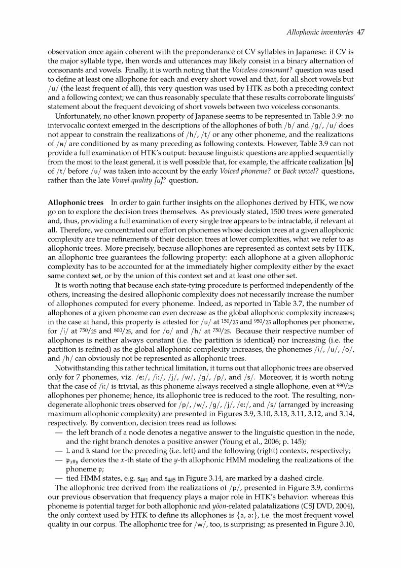
Allophonic inventories 47
observation once again coherent with the preponderance of CV syllables in Japanese: if CV isthe major syllable type, then words and utterances may likely consist in a binary alternation ofconsonants and vowels. Finally, it is worth noting that the Voiceless consonant? question was usedto define at least one allophone for each and every short vowel and that, for all short vowels but/u/ (the least frequent of all), this very question was used by HTK as both a preceding contextand a following context; we can thus reasonably speculate that these results corroborate linguists’statement about the frequent devoicing of short vowels between two voiceless consonants.
Unfortunately, no other known property of Japanese seems to be represented in Table 3.9: nointervocalic context emerged in the descriptions of the allophones of both /b/ and /g/, /u/ doesnot appear to constrain the realizations of /h/, /t/ or any other phoneme, and the realizationsof /ð/ are conditioned by as many preceding as following contexts. However, Table 3.9 can notprovide a full examination of HTK’s output: because linguistic questions are applied sequentiallyfrom the most to the least general, it is well possible that, for example, the affricate realization [ţ]of /t/ before /u/ was taken into account by the early Voiced phoneme? or Back vowel? questions,rather than the late Vowel quality [u]? question.
Allophonic trees In order to gain further insights on the allophones derived by HTK, we nowgo on to explore the decision trees themselves. As previously stated, 1500 trees were generatedand, thus, providing a full examination of every single tree appears to be intractable, if relevant atall. Therefore, we concentrated our effort on phonemeswhose decision trees at a given allophoniccomplexity are true refinements of their decision trees at lower complexities, what we refer to asallophonic trees. More precisely, because allophones are represented as context sets by HTK,an allophonic tree guarantees the following property: each allophone at a given allophoniccomplexity has to be accounted for at the immediately higher complexity either by the exactsame context set, or by the union of this context set and at least one other set.It is worth noting that because each state-tying procedure is performed independently of the
others, increasing the desired allophonic complexity does not necessarily increase the numberof allophones computed for every phoneme. Indeed, as reported in Table 3.7, the number ofallophones of a given phoneme can even decrease as the global allophonic complexity increases;in the case at hand, this property is attested for /u/ at 150/25 and 950/25 allophones per phoneme,for /i/ at 750/25 and 800/25, and for /o/ and /h/ at 750/25. Because their respective number ofallophones is neither always constant (i.e. the partition is identical) nor increasing (i.e. thepartition is refined) as the global allophonic complexity increases, the phonemes /i/, /u/, /o/,and /h/ can obviously not be represented as allophonic trees.
Notwithstanding this rather technical limitation, it turns out that allophonic trees are observedonly for 7 phonemes, viz. /e:/, /i:/, /j/, /w/, /g/, /p/, and /s/. Moreover, it is worth notingthat the case of /i:/ is trivial, as this phoneme always received a single allophone, even at 990/25
allophones per phoneme; hence, its allophonic tree is reduced to the root. The resulting, non-degenerate allophonic trees observed for /p/, /w/, /g/, /j/, /e:/, and /s/ (arranged by increasingmaximum allophonic complexity) are presented in Figures 3.9, 3.10, 3.13, 3.11, 3.12, and 3.14,respectively. By convention, decision trees read as follows:— the left branch of a node denotes a negative answer to the linguistic question in the node,
and the right branch denotes a positive answer (Young et al., 2006; p. 145);— L and R stand for the preceding (i.e. left) and the following (right) contexts, respectively;— px#y denotes the x-th state of the y-th allophonic HMMmodeling the realizations of the
phoneme p;— tied HMM states, e.g. s4#1 and s4#5 in Figure 3.14, are marked by a dashed circle.The allophonic tree derived from the realizations of /p/, presented in Figure 3.9, confirms
our previous observation that frequency plays a major role in HTK’s behavior: whereas thisphoneme is potential target for both allophonic and yoon-related palatalizations (CSJ DVD, 2004),the only context used by HTK to define its allophones is a, a:, i.e. the most frequent vowelquality in our corpus. The allophonic tree for /w/, too, is surprising; as presented in Figure 3.10,
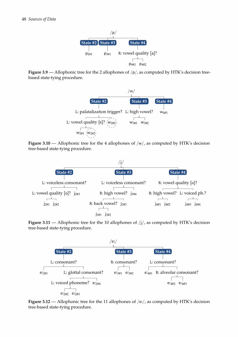
48 Sources of Data
/p/
State #4
R: vowel quality [a]?
p4#2p4#1
State #3
p3#1
State #2
p2#1
Figure 3.9—Allophonic tree for the 2 allophones of /p/, as computed by HTK’s decision tree-based state-tying procedure.
/w/
State #4
w4#1
State #3
L: high vowel?
w3#2w3#1
State #2
L: palatalization trigger?
w2#2L: vowel quality [e]?
w2#2w2#1
Figure 3.10 — Allophonic tree for the 4 allophones of /w/, as computed by HTK’s decisiontree-based state-tying procedure.
/j/
State #4
R: vowel quality [o]?
L: voiced ph.?
j4#4j4#3
R: high vowel?
j4#2j4#1
State #3
L: voiceless consonant?
j3#4R: high vowel?
j3#3R: back vowel?
j3#2j3#1
State #2
L: voiceless consonant?
j2#3L: vowel quality [o]?
j2#2j2#1
Figure 3.11 — Allophonic tree for the 10 allophones of /j/, as computed by HTK’s decisiontree-based state-tying procedure.
/e:/
State #4
L: consonant?
R: alveolar consonant?
e:4#3e:4#2
e:4#1
State #3
R: consonant?
e:3#2e:3#1
State #2
L: consonant?
L: glottal consonant?
e:2#4L: voiced phoneme?
e:2#3e:2#2
e:2#1
Figure 3.12 — Allophonic tree for the 11 allophones of /e:/, as computed by HTK’s decisiontree-based state-tying procedure.
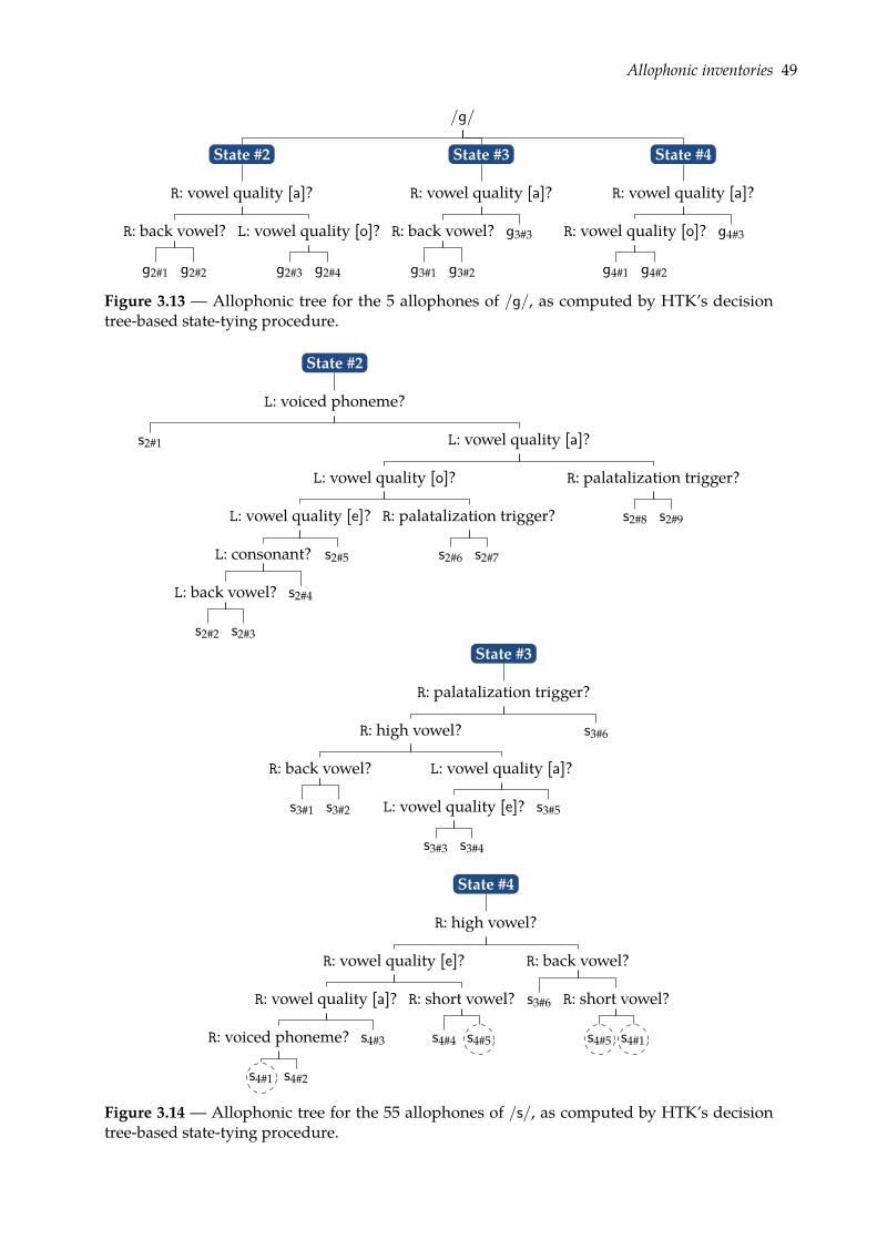
Allophonic inventories 49
/g/
State #4
R: vowel quality [a]?
g4#3R: vowel quality [o]?
g4#2g4#1
State #3
R: vowel quality [a]?
g3#3R: back vowel?
g3#2g3#1
State #2
R: vowel quality [a]?
L: vowel quality [o]?
g2#4g2#3
R: back vowel?
g2#2g2#1
Figure 3.13 — Allophonic tree for the 5 allophones of /g/, as computed by HTK’s decisiontree-based state-tying procedure.
State #2
L: voiced phoneme?
L: vowel quality [a]?
R: palatalization trigger?
s2#9s2#8
L: vowel quality [o]?
R: palatalization trigger?
s2#7s2#6
L: vowel quality [e]?
s2#5L: consonant?
s2#4L: back vowel?
s2#3s2#2
s2#1
State #3
R: palatalization trigger?
s3#6R: high vowel?
L: vowel quality [a]?
s3#5L: vowel quality [e]?
s3#4s3#3
R: back vowel?
s3#2s3#1
State #4
R: high vowel?
R: back vowel?
R: short vowel?
s4#1s4#5
s3#6
R: vowel quality [e]?
R: short vowel?
s4#5s4#4
R: vowel quality [a]?
s4#3R: voiced phoneme?
s4#2s4#1
Figure 3.14 — Allophonic tree for the 55 allophones of /s/, as computed by HTK’s decisiontree-based state-tying procedure.
50 Sources of Data
this phoneme’s realizations appear to be most constrained by preceding high or front vowels, afact that, to our knowledge, has never been discussed in the literature. Similarly, the allophonicprocesses underlying the realizations of the phoneme /j/ are unaccounted for; indeed, thevoiceness of the preceding phoneme and the height of the following vowel appear to be the mostrelevant contexts to model the different realizations of this phoneme, as attested by the repeatedusage of the questions Voiceless consonant?, Voiced phoneme?, and High vowel? in the decision treepresented in Figure 3.11. By contrast, the allophonic tree derived the long vowel /e:/ may denotea known phonemenon, though most commonly observed for short vowels, viz. vowel devoicingbetween voiceless consonants; as presented in Figure 3.12, most context sets comprise or consistin voiceless consonants as examplified by the use of the questions, Glottal consonant?, Consonant?and, to a lesser extent and by the negative, Voiced phoneme?. Although the realizations of /g/appear to be solely constrained by vowels, 6 out of 7 questions relate to the following context only,as presented in Figure 3.13; further examination of the recordings of the CSJ would be neededto determine whether the intervocalic lenition rule g→ G / V — V is attested for this phonemein the dataset. Gaining sense of all processes at stake in an allophonic tree as considerable asthe one derived for /s/ is not straightforward; however, a major feature of the phonology ofJapanese seems to be corroborated by HTK’s output: the highest-level questions defining thefollowing context of this phoneme’s realizations are Palatalization trigger? and High vowel?, onceagain confirming the ubiquity of palatalization processes in Japanese.
Data-driven linguistics All in all, although some properties of the allophonic inventories thatwere derived using HTK’s acoustics-based state-tying do relate to theoretical accounts of thephonology of Japanese, not all allophonic rules could be retrieved from the decision trees.
In our opinion, such observations do not hinder the plausibility of using allophones à la HTKto model early language acquisition. The reason for this is threefold. First, whereas the primarysource of data in HTK’s procedure is the audio recordings, most—if not all—aforementionedgrammars of the phonology of Japanese focus on articulatory descriptions of allophonic rules,relegating fine-grained acoustic considerations to the background (a notable exception beingVance, 2008). Second, we have shown that the computation of our acoustics-based allophones isheavily influenced by phoneme frequencies; thence, whereas it is surely appropriate to include arule such as h→ ç / — i in an allophonic grammar of Japanese, it is unlikely that a low-frequencyphoneme such as /h/ will have a significant weight during a global partitioning of all phones inthe CSJ. Finally, speech is the major medium by which infants receive linguistic input and, if ourallophones are acoustically different enough to be clustered in such a way by HTK, then it islikely that they are perceptually distinguishable by infants.
CHAPTER 4INDICATORS OF ALLOPHONY
Studies building upon Peperkamp et al.’s original experiments have defined various numericalcriteria that—tracking statistical regularities in a phonetically transcribed corpus—have beenused to discover which phones are actually allophones of some (yet to be discovered) phonemein the language at hand. For instance, these criteria include measures of near-complementarydistributions (Peperkamp et al., 2006; Le Calvez, 2007; Le Calvez et al., 2007; Dautriche, 2009;Martin et al., 2009; Boruta, 2009, 2011b), articulatory or acoustic similarity (Peperkamp et al., 2006;Le Calvez, 2007; Le Calvez et al., 2007; Dautriche, 2009), and, more recently, lexical dissimilarity(Martin et al., 2009; Boruta, 2009, 2011b). However, no common framework has yet been proposedto systematically define and evaluate these data-driven measures, and Peperkamp et al.’s (2006)original, distributional learner has been extended with so called constraints, filters, and cues. Inthis chapter, we show that all aforementionedmeasures indicating, to some extent, which phonesare allophones can actually be redefined as various instances of a single, cohesive concept, viz.phone-to-phone measures of dissimilarity referred to as indicators of allophony.
This chapter is divided into six main sections. In Section 4.1, we define our goals as well as theformal data structures that will be used throughout this study. Acoustic, temporal, distributionaland lexical indicators of allophony are then precisely defined in Section 4.2. Section 4.3 containsa discussion of the various standardization techniques we used so that a consistent examinationof indicators’ performance could be carried out. In Section 4.4, we present a first assessment ofindicators’ informativeness in terms of prognoses of allophony, i.e. preliminary inspections ofthe correlation between our indicators’ value and the allophony relation. Various classificationexperiments are then reported and discussed in Section 4.5. Finally, Section 4.6 contains a generalassessment of the work presented in this chapter.
4.1 Allophony: definitions and objectives
In this section, we first define the concept of indicator of allophony, as well as the mathematicalobjects we will use to represent and manipulate such indicators. We then go on to specify theobjectives of our artificial learner, viz. predicting whether or not two phones are allophones.
4.1.1 Phones, phone pairs, and allophones
As discussed in Chapter 2, the phonology of every natural language revolves around its owninventory of phonemes, i.e. a finite (and rather small) set of abstract sound categories. In turn,every phoneme can be realized by a (finite, following Assumption 3.1) number of differentphones, depending on its context. Indeed, as summarized by Lyons (1968; pp. 100–101):
the distinction between [two phones] never has the function of keeping apart differentwords [...]; it is not a functional difference: it is a phonetic difference, but not a phonological,
52 Indicators of Allophony
or phonemic, difference [...]. In cases of this kindwe say that the phonetically distinguishablepairs of speech sounds are positional variants, or allophones, of the same phoneme.~
Allophony can thus be thought of as a polyadic relation whereby allophones consist in sets ofphones brought together on the grounds that they all are realizations of the same, underlyingphoneme. To draw a non-technical analogy, the allophony relation sharesmany formal propertieswith the siblings relationship: a sibling (an allophone) is one of various inviduals (various phones)having a parent in common (having the same underlying representation). Moreover, just as thesiblings relationship may involve two or more individuals, the allophony relation may involvetwo or more phones. Indeed, we observed in Chapter 3 that not all phonemes have the samenumber of allophones (cf. Table 3.7). In fact, observing that two or more phonemes have thesame number of allophones would be nothing but a mere statistical accident.Despite this inherent property of natural languages, Peperkamp et al. (2006) introduced a
strictly pairwise computational framework whereby, for any phoneme, allophones are discoveredtwo by two. For instance, let p1, p2, p3 ⊆ P denote the phones accounting for the contextualrealizations of an hypothetical phoneme p ∈ P. In Peperkamp et al.’s framework, learning theallophony relation between these three phones amounts to learning that all three pairs p1, p2,p1, p3, and p2, p3 are each made up of two allophones. Let n ≡ |P| denote the size of a givenallophonic inventory P; put another way, the task of Peperkamp et al.’s artificial learner consistsin deciding for each of the n(n− 1)/2 possible pairs of phones whether or not the two phones itcomprises are allophones. It is worth pointing out that an additional step would be requiredto infer the phonemic inventory of the language at hand: detecting which pairs of phones areallophones is indeed insufficient to discover polyadic sets of allophones. In other words, thefact that p1 belongs to both p1, p2 and p1, p3 needs to be accounted for. In this chapter, thefocus in on Peperkamp et al.’s original pairwise allophony task. The limitations of this pairwiseapproach will be further discussed in Chapter 5 and circumvented in Chapter 6.
4.1.2 Objectives: predicting allophony
The overall goal of Peperkamp et al.’s (2006) artificial learner is to reduce the inherent variabilityin speech, represented in the present study as a set of n phones P ≡ p1, . . . , pn, to a finite setof abstract sound categories, i.e. the n phonemes P ≡ p1, . . . , pn of the target language. Let usmention that we make the trivial assumption that n > n throughout the present study, i.e. thatthere are strictly more phones than phonemes and, hence, that the problem is not already solved.Following the formal assumptions we made in Section 3.2, every phone is the realization of
one (and only one) phoneme, and every phoneme has at least one realization. Formally, we canthus define the set of phonemesP as a partition of the set of phones P. More precisely,P is a setof nonempty subsets of P such that every phone pi ∈ P belongs to exactly one of these subsets,i.e. the subset-like phonemes are both collectively exhaustive and mutually exclusive:⋃
ph = P and ph ∩ ph′ = ∅ if h 6= h′, h ∈ (1, 2, . . . , n). (4.1)Hence, under this representation of phonemes as sets, it is worth noting that the number ofallophones of a given phoneme ph is merely given by its cardinality |ph| ≥ 1.
A pairwise framework Formalizing the task introduced by Peperkamp et al. (2006), our goalis to learn an n× n symmetric Boolean matrix of allophony A ≡ [aij] where aij ∈ B denoteswhat will be referred to as the allophonic status of the pair of phones pi, pj ⊆ P. If aij = 1,the pair pi, pj is said to be allophonic (i.e. pi and pj are allophones) and, otherwise, it is saidto be non-allophonic (pi and pj are not allophones). The true, reference allophonic statuses canbe derived from the phonemic partition P of P into a reference matrix of allophony A∗ ≡ [a∗ij]whose values are given by
a∗ij ≡ J∃ h ∈ (1, 2, . . . , n), pi, pj ⊆ phK (4.2)where J · K, the evaluation function, denotes a number that is 1 if the condition within the doublebrackets is satisfied, and 0 otherwise.
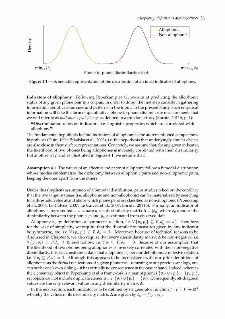
Allophony: definitions and objectives 53
mini<j δij maxi<j δijPhone-to-phone dissimilarities in ∆
Den
sity
AllophonicNon-allophonic
Figure 4.1— Schematic representation of the distribution of an ideal indicator of allophony.
Indicators of allophony Following Peperkamp et al., we aim at predicting the allophonicstatus of any given phone pair in a corpus. In order to do so, the first step consists in gatheringinformation about various cues and patterns in the input. In the present study, such empiricalinformation will take the form of quantitative, phone-to-phone dissimilarity measurements thatwe will refer to as indicators of allophony, as defined in a previous study (Boruta, 2011b; p. 1):
Discrimination relies on indicators, i.e. linguistic properties which are correlated withallophony.~
The fundamental hypothesis behind indicators of allophony is the aforementioned compactnesshypothesis (Duin, 1999; Pękalska et al., 2003), i.e. the hypothesis that underlyingly similar objectsare also close in their surface representations. Concretely, we assume that, for any given indicator,the likelihood of two phones being allophones is inversely correlated with their dissimilarity.Put another way, and as illustrated in Figure 4.1, we assume that:
Assumption 4.1 The values of an effective indicator of allophony follow a bimodal distributionwhose modes emblematize the dichotomy between allophonic pairs and non-allophonic pairs,keeping the ones apart from the others.
Under this (implicit) assumption of a bimodal distribution, prior studies relied on the corollarythat the two target statuses (i.e. allophonic and non-allophonic) can be materialized by searchingfor a threshold value at and abovewhich phone pairs are classified as non-allophonic (Peperkampet al., 2006; Le Calvez, 2007; Le Calvez et al., 2007; Boruta, 2011b). Formally, an indicator ofallophony is represented as a square n× n dissimilarity matrix ∆ ≡ [δij] where δij denotes thedissimilarity between the phones pi and pj, as estimated from observed data.Allophony is, by definition, a symmetric relation, i.e. ∀ pi, pj ⊆ P, a∗ij ⇒ a∗ji. Therefore,
for the sake of simplicity, we require that the dissimilarity measures given by any indicatorbe symmetric, too, i.e. ∀ pi, pj ⊆ P, δij = δji. Moreover, because of technical reasons to bediscussed in Chapter 6, we also require that every dissimilarity matrix ∆ be non-negative, i.e.∀ pi, pj ⊆ P, δij ≥ 0, and hollow, i.e. ∀ pi ⊆ P, δii = 0. Because of our assumption thatthe likelihood of two phones being allophones is inversely correlated with their non-negativedissimilarity, this last constraint entails that allophony is, per our definitions, a reflexive relation,i.e. ∀ pi ⊆ P, a∗ii = 1. Although this appears to be inconsistent with our prior definitions ofallophones as the distinct realizations of a given phoneme—returning to our previous analogy, onecan not be one’s own sibling—it has virtually no consequence in the case at hand. Indeed, whereasthe elementary object in Peperkamp et al.’s framework is a pair of phones pi ∪ pj = pi, pj,set objects can not include duplicate elements, i.e. pi∪ pi = pi. Consequently, off-diagonalvalues are the only relevant values in any dissimilarity matrix ∆.
In the next section, each indicator is to be defined by its generator function f : P× P→ R+
whereby the values of its dissimilarity matrix ∆ are given by δij = f (pi, pj).
54 Indicators of Allophony
4.2 Building indicators of allophony
Before turning to the actual definitions, let us revisit the nature and the form of the data that areavailable to us in order to build indicators of allophony. On one hand, we can rely on acoustics-based allophonic HMMs modeling the realizations of every single phone in the CSJ and, on theother hand, we can monitor statistical patterns in a phonetic transcription of the CSJ where datahave been coded at three different linguistic levels: phones, words, and utterances (cf. Chapter 3).For the sake of brevity, indicators of allophony are insignificantly defined in this section as
either similarity or dissimilarity measures; standardization issues will be discussed in Section 4.3.Furthermore, it is worthmentioning that each indicator’s name includes a prefix blackboard-boldletter reminiscent of the type of information this indicator relies on: A for acoustic indicators, T
for temporal indicators, D for distributional indicators, and L for lexical indicators.
4.2.1 Acoustic indicators
In this section, we describe the computation of two indicators relying on measures of the acousticdissimilarity between phones. Although the relevance of phonetic criteria for the definition ofphonemes has been discussed and, enventually, minimized in favor of an emphasis on distribu-tional and functional criteria (Trubetzkoy, 1939; Austin, 1957), we reiterate our argument thatdisregarding actual sounds in a study of sound categories would appear to be contrieved. More-over, and as previously stated, speech is the major medium by which infants receive linguisticinput. We therefore consider acoustic information to be a legitimate cue to keep track of.
Prior scholarship Using the data at hand, the act of measuring the acoustic dissimilaritybetween two phones amounts to measuring the dissimilarity between the two allophonic HMMsthat were trained to model their actual realizations in the recordings of the CSJ. We will thusfocus in the present study on the measure of acoustic dissimilarity described by Dautriche(2009; implementation by Dupoux & Schatz, priv. comm.), for the sake of comparability—eventhough various seminal acoustic distance measures have been defined (e.g. Gray & Markel, 1976;Mermelstein, 1976; Everson & Penzhorn, 1988; Mak & Barnard, 1996). For this particular measureas in Section 3.2.2, it is worth noting that the following protocol is not ours; it is only presentedhere in order to ensure the reproducibility of the results to be presented in subsequent sections.
Concretely, Dautriche (2009) defined the acoustic dissimilarity between two phones pi, pj ⊆P as the dissimilarity between their respective HMMs. In that study, the latter dissimilarityis given by the dynamic time warping between the two sequences si and sj made up of theirrespective emitting states, and using a symmetrization of the Kullback–Leibler divergencebetween the states’ output probability density functions as the local distance function. Thegenerator function of this indicator, which will be referred to as A-DTW, is given by
A-DTW(pi, pj) ≡ DTW(si, sj; SKLD) (4.3)where SKLD denotes Dautriche’s symmetrization of the Kullback–Leibler divergence (to beprecisely defined hereafter), and DTW(x, y; f ) denotes the value of the optimal symmetricdynamic time warping that completely maps the sequences x and y onto one another using f asthe local distance (Sakoe & Chiba, 1978; Giorgino, 2009). Here, dynamic time warping is used tofind the optimal path among all paths from both HMMs’ first emitting states to both HMMs’last emitting states. The search space of all such possible paths is illustrated in the lattice-likestructure in Figure 4.2.Dautriche’s symmetrized Kullback–Leibler divergence is a straightforward extension of the
original Kullback–Leibler divergence (henceforth KLD; Kullback & Leibler, 1951), a seminalmeasure of dissimilarity between two probability density functions. For two arbitrary densityfunctions f (x) and f ′(x), their KLD is given by
KLD( f ‖ f ′) ≡∫
f (x) logf (x)f ′(x)
dx (4.4)
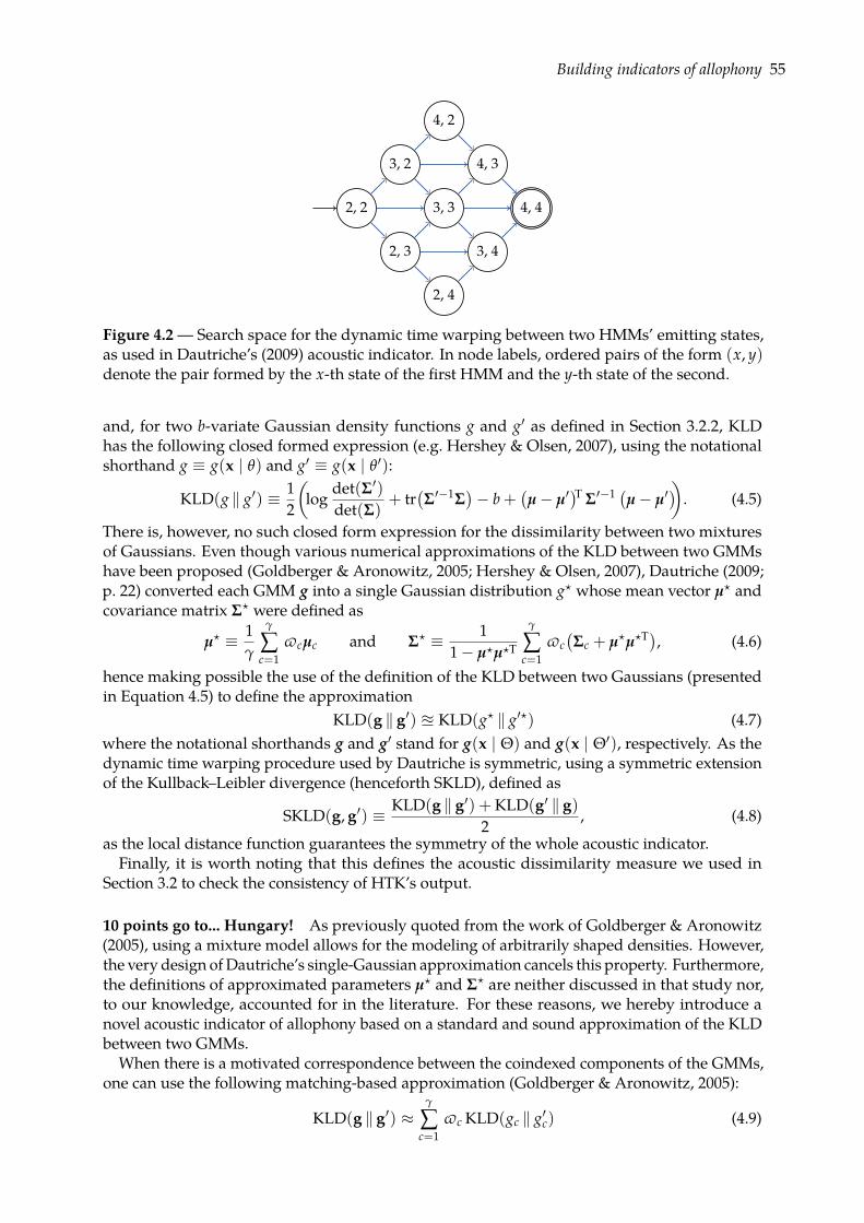
Building indicators of allophony 55
2, 2
2, 3
2, 4
3, 2
3, 3
3, 4
4, 2
4, 3
4, 4
Figure 4.2— Search space for the dynamic time warping between two HMMs’ emitting states,as used in Dautriche’s (2009) acoustic indicator. In node labels, ordered pairs of the form (x, y)denote the pair formed by the x-th state of the first HMM and the y-th state of the second.
and, for two b-variate Gaussian density functions g and g′ as defined in Section 3.2.2, KLDhas the following closed formed expression (e.g. Hershey & Olsen, 2007), using the notationalshorthand g ≡ g(x | θ) and g′ ≡ g(x | θ′):
KLD(g ‖ g′) ≡ 12
(log
det(Σ′)det(Σ)
+ tr(Σ′−1Σ
)− b +
(µ− µ′
)T Σ′−1 (µ− µ′))
. (4.5)
There is, however, no such closed form expression for the dissimilarity between two mixturesof Gaussians. Even though various numerical approximations of the KLD between two GMMshave been proposed (Goldberger & Aronowitz, 2005; Hershey & Olsen, 2007), Dautriche (2009;p. 22) converted each GMM g into a single Gaussian distribution g? whose mean vector µ? andcovariance matrix Σ? were defined as
µ? ≡ 1γ
γ
∑c=1
vcµc and Σ? ≡ 11− µ?µ?T
γ
∑c=1
vc(Σc + µ?µ?T), (4.6)
hence making possible the use of the definition of the KLD between two Gaussians (presentedin Equation 4.5) to define the approximation
KLD(g ‖ g′) u KLD(g? ‖ g′?) (4.7)where the notational shorthands g and g′ stand for g(x | Θ) and g(x | Θ′), respectively. As thedynamic time warping procedure used by Dautriche is symmetric, using a symmetric extensionof the Kullback–Leibler divergence (henceforth SKLD), defined as
SKLD(g, g′) ≡ KLD(g ‖ g′) + KLD(g′ ‖ g)2
, (4.8)
as the local distance function guarantees the symmetry of the whole acoustic indicator.Finally, it is worth noting that this defines the acoustic dissimilarity measure we used in
Section 3.2 to check the consistency of HTK’s output.
10 points go to... Hungary! As previously quoted from the work of Goldberger & Aronowitz(2005), using a mixture model allows for the modeling of arbitrarily shaped densities. However,the very design ofDautriche’s single-Gaussian approximation cancels this property. Furthermore,the definitions of approximated parameters µ? and Σ? are neither discussed in that study nor,to our knowledge, accounted for in the literature. For these reasons, we hereby introduce anovel acoustic indicator of allophony based on a standard and sound approximation of the KLDbetween two GMMs.
When there is a motivated correspondence between the coindexed components of the GMMs,one can use the following matching-based approximation (Goldberger & Aronowitz, 2005):
KLD(g ‖ g′) ≈γ
∑c=1
vc KLD(gc ‖ g′c) (4.9)
56 Indicators of Allophony
However, to our knowledge, we can not assume any correspondence between coindexed mixturecomponents in the GMMs produced by HTK (Young et al., 2006; pp. 156–157). Therefore, priorto approximating the KLD between two GMMs as the weighted sum of the KLDs between theircomponents, we need to specify how to pair each component of one GMM with one componentof the other. Goldberger & Aronowitz highlighted the fact that any permutation of a givenGMM’s components yields the exact same mixture of the probability density functions. Putanother way, two GMMs g and g with equal parameter values but different component orderingactually define the same probability density function. Relying on this property, they defined thefollowing approximation (Goldberger & Aronowitz, 2005; eq. 3):
KLD(g ‖ g′) ≈ ming′∈℘(g′)
γ
∑c=1
vc KLD(gc ‖ g′c), (4.10)
where ℘(g′) denotes the set of all possible permutations of the γ components in the mixture g′,and g′c denotes the c-th component of the permuted mixture g′. A naive implementation of thismatching-based approximation would require searching through all |℘(g′)| = γ! possible per-mutations of the components (i.e. 17! ≈ 3.5 · 1014 permutations in the case at hand). However, aswith any instance of the assignment problem, this search can be solved in only O(γ3) operations(i.e. 173 = 4913 operations, where O denotes the asymptotic upper bound on an algorithm’stime complexity; Cormen et al., 2001) using the so called Hungarian method (algorithm by Kuhn,1955, and Munkres, 1957; implementation by Clapper, 2009). Using a symmetrization similar tothe one used by Dautriche (2009), we approximate the SKLD between two GMMs g and g′ as
SKLD(g, g′) u 12
ming′∈℘(g′)
γ
∑c=1
(vc KLD(gc ‖ g′c) + v′c KLD(g′c ‖ gc)
), (4.11)
that is to say using the permutation g′ that minimizes the global sum, for each component, ofthe weighted sums of the component-wise, single-Gaussian KLDs.
Finally, our novel acoustic match-based indicator of allophony, dubbed A-MBD, is defined asthe sum of the SKLDs between the coindexed emitting states of both phones’ HMMs. Formally,its generator function is given by
A-MBD(pi, pj) ≡ ∑ı∈2,3,4
SKLD(gi(ı), gj(ı)), (4.12)
where gi(ı) denotes the GMM associated to the ı-th state of the HMMmodeling the phone pi.
4.2.2 Temporal indicators
Previously defined acoustic indicators rely on the comparison of probability distributions, viz.the GMMs assigned to the emitting states of both phones’ HMMs. By doing so, the underlyingdata they examine are the acoustic features we derived with HTK. However, to a certain extent,temporal information is not immediately accessible in a HMM. Whereas transition probabilitiesbetween states constrain the (mostly left-to-right) progression in the observations’ structure (i.e.the sequence of acoustic features extracted for each phone), retrieving information about eachphone’s attested durations in the CSJ from an allophonic HMM is impossible because of thegeneralization process inherent to any paramater estimation technique.
However, gathering information concerning phone durations might prove to be useful for thediscovery of allophony. Broadly speaking, relative durations can indeed be used to define anorder on some phoneme classes: the realizations of long vowels tend to be longer than thoseof short vowels—so we hope—and vowels tend to be longer than consonants (e.g. Grønnum &Basbøll, 2003; Kewley-Port et al., 2007). Thence, comparing two phones’ duration distributionsmay indicate whether or not they are allophones. To our knowledge, duration alone has neverbeen examined a potential cue for allophony. Throughout this study, we test the hypothesis thattemporal information can be used to derive effective indicators of allophony.
Building indicators of allophony 57
Defining phonemes in terms of time In this section, we introduce a novel class of indicatorsof allophony relying on phone duration information, viz. temporal indicators. It is worth notingimmediately that, by design, such indicators would fail to account for allophonic processes thataffect the duration of their target phonemes (e.g. shortening a long vowel). However, to ourknowledge, no such length-affecting process is attested in Japanese.The main attraction of temporal indicators arises from the simplicity of the data they
manipulate—especially compared to the considerable formal apparatus needed for the def-inition of acoustic indicators. Using the data at hand, information about each sound token’sduration is readily available. Indeed, two of our recurrent concerns during the preprocessingoperations reported in Section 3.1 concerned temporal annotation. On one hand, we focused onpreserving the alignement between the original audio recordings of the CSJ and our custom-built transcription as, in the latter, this alignement is materialized by a sequence of timestampsmarking the beginning and the end of each and every phone in the corpus. On the other hand,we successfully checked that all phones in the dataset have non-negative durations.
All temporal indicators to be defined hereafter rely on the same logic at the computationallevel (Marr, 1982). First, for each phone pi ∈ P, the exhaustive list of its attested durationsare collected in the vector ti. Then, we assess the temporal dissimilarity between two phonespi, pj ∈ P by comparing the value of a given statistic about each phone’s duration vector ti andtj. More precisely, given a scalar function f , we define the temporal dissimilarity T- f betweentwo phones pi and pj as
T- f (pi, pj) ≡ duratio(pi, pj; f ) with duratio(pi, pj; f ) ≡ min f (ti), f (tj)max f (ti), f (tj)
, (4.13)
where the minimum-over-maximum ratio guarantees the symmetry of all temporal indicators.We now go on to instantiate four temporal indicators of allophony, specifying a different
function f for each of them.
Duration tendency The first two temporal indicators we consider in the present study rely onmeasures of central tendency, i.e. estimates of the average duration aroundwhich a given phone’sdurations tend to cluster. Though many measures of central tendency have been proposed inthe field of descriptive statistics, we only define and evaluate two of them (the inclusion criteriawill be discussed hereafter). First, because it is a ubiquitous estimator of central tendency, wedefine a temporal indicator that relies on a comparison of the arithmetic means of both phones’duration vectors. Referred to as T-mean, its generator function is given by
T-mean(pi, pj) ≡ duratio(pi, pj; mean) with mean(t) ≡ 1|t||t|∑ι=1
tι. (4.14)
In spite of its popularity, the arithmetic mean has one major limitation: it is highly sensitive tooutliers (i.e. extreme values), in the sense that it yields an arbitrarily large estimate of centraltendency if the sample contains an arbitrarily large observation. By contrast, the median is oneof the most robust estimators of central tendency (Rousseeuw & Croux, 1992, 1993). Therefore,we also introduce a temporal indicator, dubbed T-median, that relies on the comparison of bothphones’ median duration. Its generator is given by
T-median(pi, pj) ≡ duratio(pi, pj; median) with median(t) ≡ t|t|/2, (4.15)assuming, for the sake of simplicity, that the values in the duration vector t are arranged inincreasing order.
Duration dispersion The second type of temporal indicators we will examine in the presentstudy rely on measures of statistical dispersion, i.e. estimates of the variability of a given phone’sdurations. Following the same argument as before, we introduce both a well-known (yet notrobust) temporal indicator, and a robust (yet less ubiquitous) indicator. The first dispersion-basedtemporal indicator we define relies on a comparison of the standard deviations of both phones’
58 Indicators of Allophony
durations. Referred to as T-stdev, its generator function is defined as
T-stdev(pi, pj) ≡ duratio(pi, pj; stdev) with stdev(t) ≡
√√√√ 1|t||t|∑ι=1
(tι −mean(t))2. (4.16)
Because it relies on the arithmetic mean, standard deviation suffers the same sensitivity tooutliers. Mirkin (2005; p. 65) recommends using the range (i.e. the difference between the highestand the lowest values) a simple yet effective estimator of dispersion, even though it amountsto comparing the most extreme values in the sample. The generator function of correspondingtemporal indicator, dubbed T-range, is straightforwardly given by
T-range(pi, pj) ≡ duratio(pi, pj; T-range) with range(t) ≡ max(t)−min(t). (4.17)
Population control As discussed in the first section of this chapter, the major assumptionbehind indicators of allophony is that their values follow a bimodal distribution whose modeskeep apart allophonic pairs from non-allophonic pairs. Consequently, the relative ranks ofan indicator’s values may matter more than the values themselves. Therefore, any indicatorof allophony whose generator function can be defined as a rank-preserving (i.e. monotonic)transformation of another indicator’s generator functionwould yield the exact same observations,at least as far as allophony is concerned. For example, the standard deviation of a given sampleis by definition equal to the square root of its variance: as the square root function is monotonic,we know in advance that both statistics would yield identical indicators. For this reason, and forthe sake of brevity, we limit our examination of the relevance of temporal information for thediscovery of allophony to the aforementioned temporal indicators.
4.2.3 Distributional indicators
Acoustic and temporal indicators of allophony rely on the examination of sound tokens, inthe sense that their values depend on the properties of every instance of every allophone ofevery phoneme in the corpus. In other words, one could argue that our previous assumptionof a quantized input (cf. Assumption 3.1) would have been dispensable, as far as acoustic andtemporal indicators are concerned. Our answer to this potential objection is that we build uponthe work of Peperkamp et al. (2006). As we argued in Section 3.2, only a quantized input allowsfor the collection of statiscal information about every phone’s context distribution, the very datatheir artificial learner examines.
In this section, we present the various distributional indicators of allophony used throughoutthe present study, i.e. indicators whose definition is based on a statistical assessment of phoneco-occurrence patterns. Even though Peperkamp et al.’s (2006) study contains, chronologicallyspeaking, the first account of a distributional learner of allophony (notwithstanding early workon successor counts byHarris, 1951), we base the following exposition on the extended discussiongiven in Le Calvez’s (2007; pp. 23–52) dissertation.
Complementary distributions The major idea behind Peperkamp et al.’s (2006) model of theacquisition of allophonic rules is to take advantage of the observation that the allophones of agiven phoneme have non-overlapping distributions (Peperkamp & Dupoux, 2002). Consider,for example, the aforementioned allophonic palatalization rule in Japanese whereby the alve-olar consonant /s/ is realized as an post-alveolar [S] before the high vowel /i/, i.e. s→ S / — i(Miller, 1967). By virtue of this rule, the words /miso/ and /mosi/ are to be realized as [miso](“miso,” a traditional Japanese seasoning) and [moSi] (as in [moSimoSi], “hello,” when answeringa telephone), respectively. Whereas [S] only occurs before (realizations of) /i/, [s] appears in allother contexts. Because, [S] and [s] occur in distinct contexts, they are said to have complementarydistributions and are thus potential allophones. What is also true for previously discussed lin-guistic cues of allophony is that complementary distribution is not a sufficient criterion for thediscovery of allophony, as highlighted by Peperkamp et al. (2006; p. B33):
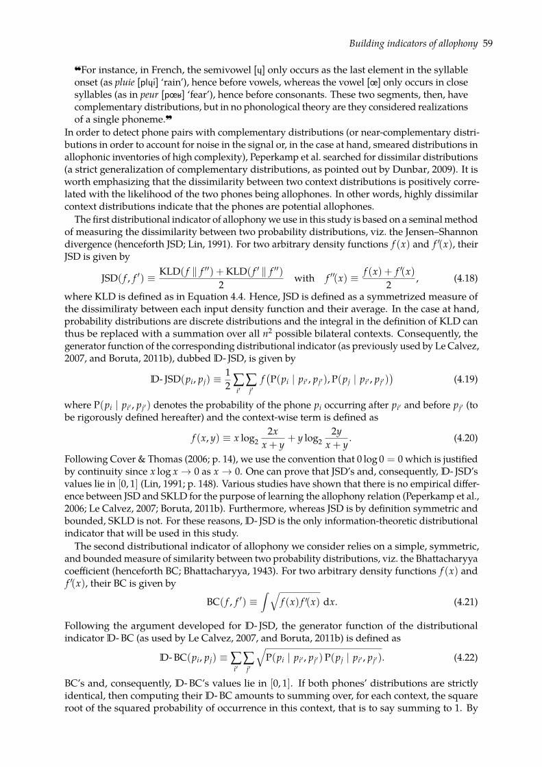
Building indicators of allophony 59
For instance, in French, the semivowel [4] only occurs as the last element in the syllableonset (as pluie [pl4i] ‘rain’), hence before vowels, whereas the vowel [œ] only occurs in closesyllables (as in peur [pœK] ‘fear’), hence before consonants. These two segments, then, havecomplementary distributions, but in no phonological theory are they considered realizationsof a single phoneme.~
In order to detect phone pairs with complementary distributions (or near-complementary distri-butions in order to account for noise in the signal or, in the case at hand, smeared distributions inallophonic inventories of high complexity), Peperkamp et al. searched for dissimilar distributions(a strict generalization of complementary distributions, as pointed out by Dunbar, 2009). It isworth emphasizing that the dissimilarity between two context distributions is positively corre-lated with the likelihood of the two phones being allophones. In other words, highly dissimilarcontext distributions indicate that the phones are potential allophones.
The first distributional indicator of allophonywe use in this study is based on a seminalmethodof measuring the dissimilarity between two probability distributions, viz. the Jensen–Shannondivergence (henceforth JSD; Lin, 1991). For two arbitrary density functions f (x) and f ′(x), theirJSD is given by
JSD( f , f ′) ≡ KLD( f ‖ f ′′) + KLD( f ′ ‖ f ′′)2
with f ′′(x) ≡ f (x) + f ′(x)2
, (4.18)
where KLD is defined as in Equation 4.4. Hence, JSD is defined as a symmetrized measure ofthe dissimiliraty between each input density function and their average. In the case at hand,probability distributions are discrete distributions and the integral in the definition of KLD canthus be replaced with a summation over all n2 possible bilateral contexts. Consequently, thegenerator function of the corresponding distributional indicator (as previously used by Le Calvez,2007, and Boruta, 2011b), dubbed D- JSD, is given by
D- JSD(pi, pj) ≡12 ∑
i′∑j′
f(P(pi | pi′ , pj′), P(pj | pi′ , pj′)
)(4.19)
where P(pi | pi′ , pj′) denotes the probability of the phone pi occurring after pi′ and before pj′ (tobe rigorously defined hereafter) and the context-wise term is defined as
f (x, y) ≡ x log22x
x + y+ y log2
2yx + y
. (4.20)
Following Cover & Thomas (2006; p. 14), we use the convention that 0 log 0 = 0 which is justifiedby continuity since x log x → 0 as x → 0. One can prove that JSD’s and, consequently, D- JSD’svalues lie in [0, 1] (Lin, 1991; p. 148). Various studies have shown that there is no empirical differ-ence between JSD and SKLD for the purpose of learning the allophony relation (Peperkamp et al.,2006; Le Calvez, 2007; Boruta, 2011b). Furthermore, whereas JSD is by definition symmetric andbounded, SKLD is not. For these reasons, D- JSD is the only information-theoretic distributionalindicator that will be used in this study.The second distributional indicator of allophony we consider relies on a simple, symmetric,
and boundedmeasure of similarity between two probability distributions, viz. the Bhattacharyyacoefficient (henceforth BC; Bhattacharyya, 1943). For two arbitrary density functions f (x) andf ′(x), their BC is given by
BC( f , f ′) ≡∫ √
f (x) f ′(x) dx. (4.21)
Following the argument developed for D- JSD, the generator function of the distributionalindicator D- BC (as used by Le Calvez, 2007, and Boruta, 2011b) is defined as
D- BC(pi, pj) ≡∑i′
∑j′
√P(pi | pi′ , pj′)P(pj | pi′ , pj′). (4.22)
BC’s and, consequently, D- BC’s values lie in [0, 1]. If both phones’ distributions are strictlyidentical, then computing their D- BC amounts to summing over, for each context, the squareroot of the squared probability of occurrence in this context, that is to say summing to 1. By
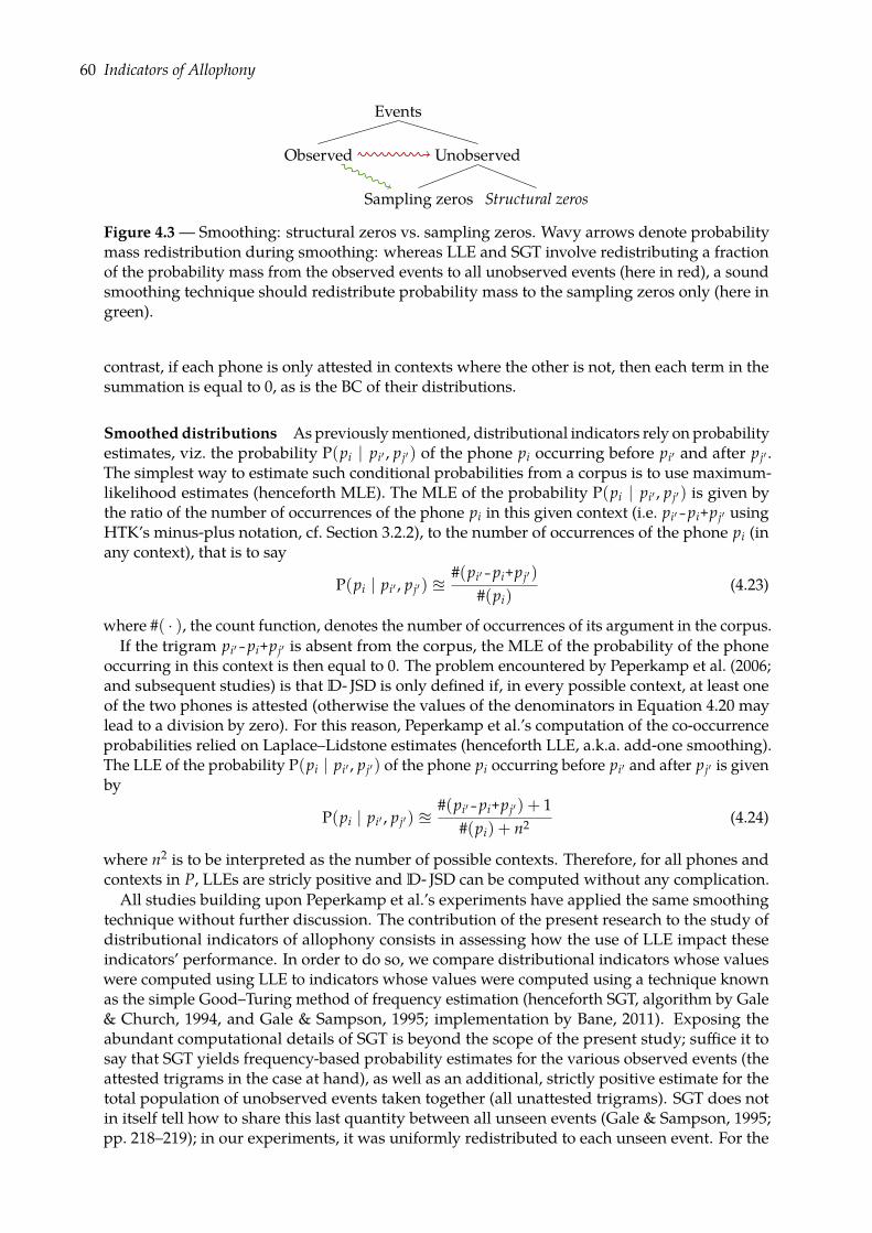
60 Indicators of Allophony
Events
Unobserved
Structural zerosSampling zeros
Observed
Figure 4.3— Smoothing: structural zeros vs. sampling zeros. Wavy arrows denote probabilitymass redistribution during smoothing: whereas LLE and SGT involve redistributing a fractionof the probability mass from the observed events to all unobserved events (here in red), a soundsmoothing technique should redistribute probability mass to the sampling zeros only (here ingreen).
contrast, if each phone is only attested in contexts where the other is not, then each term in thesummation is equal to 0, as is the BC of their distributions.
Smoothed distributions As previouslymentioned, distributional indicators rely on probabilityestimates, viz. the probability P(pi | pi′ , pj′) of the phone pi occurring before pi′ and after pj′ .The simplest way to estimate such conditional probabilities from a corpus is to use maximum-likelihood estimates (henceforth MLE). The MLE of the probability P(pi | pi′ , pj′) is given bythe ratio of the number of occurrences of the phone pi in this given context (i.e. pi′-pi+pj′ usingHTK’s minus-plus notation, cf. Section 3.2.2), to the number of occurrences of the phone pi (inany context), that is to say
P(pi | pi′ , pj′) u#(pi′-pi+pj′)
#(pi)(4.23)
where #( · ), the count function, denotes the number of occurrences of its argument in the corpus.If the trigram pi′-pi+pj′ is absent from the corpus, the MLE of the probability of the phone
occurring in this context is then equal to 0. The problem encountered by Peperkamp et al. (2006;and subsequent studies) is that D- JSD is only defined if, in every possible context, at least oneof the two phones is attested (otherwise the values of the denominators in Equation 4.20 maylead to a division by zero). For this reason, Peperkamp et al.’s computation of the co-occurrenceprobabilities relied on Laplace–Lidstone estimates (henceforth LLE, a.k.a. add-one smoothing).The LLE of the probability P(pi | pi′ , pj′) of the phone pi occurring before pi′ and after pj′ is givenby
P(pi | pi′ , pj′) u#(pi′-pi+pj′) + 1
#(pi) + n2 (4.24)
where n2 is to be interpreted as the number of possible contexts. Therefore, for all phones andcontexts in P, LLEs are stricly positive and D- JSD can be computed without any complication.All studies building upon Peperkamp et al.’s experiments have applied the same smoothing
technique without further discussion. The contribution of the present research to the study ofdistributional indicators of allophony consists in assessing how the use of LLE impact theseindicators’ performance. In order to do so, we compare distributional indicators whose valueswere computed using LLE to indicators whose values were computed using a technique knownas the simple Good–Turing method of frequency estimation (henceforth SGT, algorithm by Gale& Church, 1994, and Gale & Sampson, 1995; implementation by Bane, 2011). Exposing theabundant computational details of SGT is beyond the scope of the present study; suffice it tosay that SGT yields frequency-based probability estimates for the various observed events (theattested trigrams in the case at hand), as well as an additional, strictly positive estimate for thetotal population of unobserved events taken together (all unattested trigrams). SGT does notin itself tell how to share this last quantity between all unseen events (Gale & Sampson, 1995;pp. 218–219); in our experiments, it was uniformly redistributed to each unseen event. For the
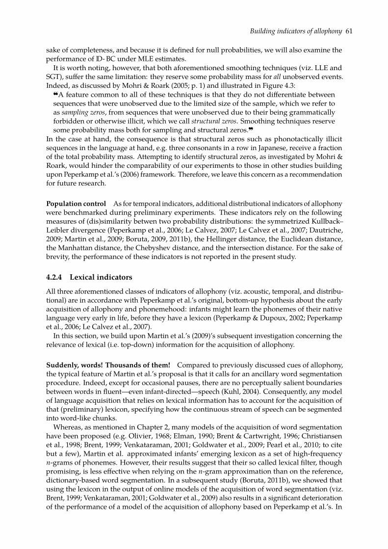
Building indicators of allophony 61
sake of completeness, and because it is defined for null probabilities, we will also examine theperformance of D- BC under MLE estimates.
It is worth noting, however, that both aforementioned smoothing techniques (viz. LLE andSGT), suffer the same limitation: they reserve some probability mass for all unobserved events.Indeed, as discussed by Mohri & Roark (2005; p. 1) and illustrated in Figure 4.3:
A feature common to all of these techniques is that they do not differentiate betweensequences that were unobserved due to the limited size of the sample, which we refer toas sampling zeros, from sequences that were unobserved due to their being grammaticallyforbidden or otherwise illicit, which we call structural zeros. Smoothing techniques reservesome probability mass both for sampling and structural zeros.~
In the case at hand, the consequence is that structural zeros such as phonotactically illicitsequences in the language at hand, e.g. three consonants in a row in Japanese, receive a fractionof the total probability mass. Attempting to identify structural zeros, as investigated by Mohri &Roark, would hinder the comparability of our experiments to those in other studies buildingupon Peperkamp et al.’s (2006) framework. Therefore, we leave this concern as a recommendationfor future research.
Population control As for temporal indicators, additional distributional indicators of allophonywere benchmarked during preliminary experiments. These indicators rely on the followingmeasures of (dis)similarity betwen two probability distributions: the symmetrized Kullback–Leibler divergence (Peperkamp et al., 2006; Le Calvez, 2007; Le Calvez et al., 2007; Dautriche,2009; Martin et al., 2009; Boruta, 2009, 2011b), the Hellinger distance, the Euclidean distance,the Manhattan distance, the Chebyshev distance, and the intersection distance. For the sake ofbrevity, the performance of these indicators is not reported in the present study.
4.2.4 Lexical indicators
All three aforementioned classes of indicators of allophony (viz. acoustic, temporal, and distribu-tional) are in accordance with Peperkamp et al.’s original, bottom-up hypothesis about the earlyacquisition of allophony and phonemehood: infants might learn the phonemes of their nativelanguage very early in life, before they have a lexicon (Peperkamp & Dupoux, 2002; Peperkampet al., 2006; Le Calvez et al., 2007).
In this section, we build upon Martin et al.’s (2009)’s subsequent investigation concerning therelevance of lexical (i.e. top-down) information for the acquisition of allophony.
Suddenly, words! Thousands of them! Compared to previously discussed cues of allophony,the typical feature of Martin et al.’s proposal is that it calls for an ancillary word segmentationprocedure. Indeed, except for occasional pauses, there are no perceptually salient boundariesbetween words in fluent—even infant-directed—speech (Kuhl, 2004). Consequently, any modelof language acquisition that relies on lexical information has to account for the acquisition ofthat (preliminary) lexicon, specifying how the continuous stream of speech can be segmentedinto word-like chunks.Whereas, as mentioned in Chapter 2, many models of the acquisition of word segmentation
have been proposed (e.g. Olivier, 1968; Elman, 1990; Brent & Cartwright, 1996; Christiansenet al., 1998; Brent, 1999; Venkataraman, 2001; Goldwater et al., 2009; Pearl et al., 2010; to citebut a few), Martin et al. approximated infants’ emerging lexicon as a set of high-frequencyn-grams of phonemes. However, their results suggest that their so called lexical filter, thoughpromising, is less effective when relying on the n-gram approximation than on the reference,dictionary-based word segmentation. In a subsequent study (Boruta, 2011b), we showed thatusing the lexicon in the output of online models of the acquisition of word segmentation (viz.Brent, 1999; Venkataraman, 2001; Goldwater et al., 2009) also results in a significant deteriorationof the performance of a model of the acquisition of allophony based on Peperkamp et al.’s. In
62 Indicators of Allophony
another study (Boruta, 2009; Boruta et al., 2011), we showed that the same models of wordsegmentation do not resist an increase in allophonic complexity: as the allophonic complexityof their input increases, their performance tends to that of baseline models that insert wordboundaries at random in an unsegmented corpus.
For these reasons, we rely on the dictionary-based segmentation provided in theCSJ to computethe values of all lexical indicators to be defined hereafter. Formally, we represent the lexiconL as a finite set of words L ≡ w1, . . . ,wl, associated to their respective relative frequenciesF ≡ f1, . . . , fl. Additionally, let L` and |w| denote the sublexicon of words of length ` and thelength of the word w, respectively.
Terminimal pairs Martin et al.’s lexicon-based learner of allophony is based on the observationthat the application of allophonic rules in the vicinity of word boundaries may create minimallydifferent word forms. Consequently, repeating our prior example concerning the allophonicrule of voicing in Mexican Spanish whereby /s/ is realized as [z] before voiced consonants,i.e. [feliz nabidad] ∼ [felis kumpleaños] (“happy Christmas” ∼ “happy birthday”), the intuitionis that tracking contrasts on the first or last segment of otherwise identical word forms suchas [feliz] ∼ [felis] (which is not a minimal pair stricto sensu) may be relevant in order to learnallophonic rules. In order to distinguish such word pairs from true minimal pairs (i.e. comprisingdistinct words) such as /felis/∼ /relis/ (“happy”∼ “landslide”, also inMexican Spanish), we willrefer to the former as terminimal pairs, following the terminology used in a prior study (Boruta,2009; pp. 38–39).
The more the merrier Martin et al.’s (2009) proposal is actually twofold. Not only do they relyon terminimal pairs, they also rely on word length. As they observed, the frequency distributionof word lengths follows a power law (i.e. most words are very short and few words are verylong) and, as a consequence, searching for terminimal pairs in very short words tend to generatemany false alarms. In order to account for this observation, Martin et al. set ad hoc bounds onthe length of the words they actually considered in their study; for instance, words less than 4phoneme-long were discarded. More surprisingly, they also introduced an upper bound: wordsless than 8 phoneme-long were discarded, too, on the grounds that they occur too infrequently tobe informative. Althoughwe consider Martin et al.’s argument about the limited informativenessof very shorts words to be acceptable, we do not endorse their views on long words. Whereasit is indeed unlikely that many terminimal pairs be attested on words of, for example, length10, setting an upper bound on word length amounts to denying oneself the access to preciousinformation in the eventuality of such a lexical contrast. The only word length to be trulyirrelevant for the search of terminimal pairs is ` = 1. Indeed, by definition, all words of length` = 1 form terminimal pairs as they contain no linguistic material apart from their contrastinginitial-and-final phone.The first lexical indicator of allophony to be considered in this study is a mere reformulation
of Martin et al.’s so called lexical filter albeit, for the aforementioned reasons, using all wordsin the lexicon but those comprising a single phone. This indicator, dubbed L-BTP, relies on aBoolean function whose value for a given phone pair pi, pj ⊆ P is 1 if the lexicon L contains atleast one terminimal pair of words contrasting on these phones, and 0 otherwise. Formally, itsgenerator function is given by
L-BTP(pi, pj) ≡ J∃ wı,w ⊆ L, |wı| > 1∧ |w| > 1∧ TP(wı,w, pi, pj)K (4.25)where TP(w,w′, p, p′) is 1 if and only if the words w and w′ for a terminimal pair contrasting onthe phones p and p′. It is worth noting that this indicator is included in the present study solelyfor the sake of comparability with Martin et al.’s experiments.Indeed, we showed (Boruta, 2011b) that the utterly limited number of values that L-BTP can
take, i.e. 0, 1, hinders its performance as, for any given phone pair, a single false alarm wouldswitch its value to 1. Therefore, we introduce a simple yet more descriptive lexical indicator of
Numerical recipes 63
allophony, dubbed L-NTP, whose generator function amounts to tallying, for a given phonepair, the number of terminimal pairs contrasting on those phones, that is to say
L-NTP(pi, pj) ≡∞
∑`=2
|L`|∑ı=1
|L`|∑
=ı+1TP(wı,w, pi, pj). (4.26)
Incidentally, L-BTP’s generator function can be defined as a stripped-down version of L-NTP’sby virtue of the following equality:
∀ pi, pj ⊆ P, L-BTP(pi, pj) = JL-NTP(pi, pj) > 0K. (4.27)Finally, in order to investigate Martin et al.’s intuition about word length, we also consider a
length-weighted lexical indicator of allophony. Referred to as L-WTP (originally FL*; Boruta,2011b), its generator function is given by
L-WTP(pi, pj) ≡∞
∑`=2
`|L`|∑ı=1
|L`|∑
=ı+1TP(wı,w, pi, pj). (4.28)
Functional load The final indicator of allophony to be considered in this study is based onHockett’s definition of functional load (Hockett, 1955; Surendran & Niyogi, 2006). Functionalload is an information-theoretic concept that accounts for the fraction of information contentthat is lost in a language when a contrast is cancelled out. In the case of allophony, it accountsfor the fraction of information content that is lost when the contrast between two given phonesis neutralized. As argued by Lyons (1968; p. 82):
It is to be expected therefore that children will tend to learn first those contrasts whichhave the highest functional load in the language that they hear about them [...]. The precisequantification of functional load is complicated, if not made absolutely impossible [...].~
Here, we follow the definitions given by Hockett (1955) and, more recently, Surendran & Niyogi(2006) whereby the information content of the language at hand is represented by its wordentropy. Using the available data structures, the language’s word entropy H(L) is given by
H(L) ≡ −|L|∑ı=1
fı log2 fı, (4.29)
treating the lexicon as a random variable L whose events w1, . . . ,wl have probabilitesf1, . . . , fl. The generator function of the corresponding indicator, referred to as L-HFL (origi-nally HFL; Boruta, 2011b) is then defined as
L-HFL(pi, pj) ≡H(L)−H
(f (L; pi, pj)
)
H(L), (4.30)
where f (L; pi, pj) denotes Coolen et al.’s (2005) broken-typewriter function. This function returnsa new random variable identical to L except that pi and pj are indistinguishable. L-HFL(pi, pj)is thus equal to the fraction of information content that is lost when the contrast between pi andpj is neutralized. One can prove that L-HFL’s values lie in [0, 1] (Coolen et al., 2005; p. 259).
4.3 Numerical recipes
For the sake of simplicity, and as summarized in Table 4.1, we insignificantly defined indicatorsof allophony as dissimilarity (A-DTW, A-MBD, D-BC-MLE, D-BC-LLE, and D-BC-SGT) or sim-ilarity (T-mean, T-median, T-stdev, T-range, D-JSD-LLE, D-JSD-SGT, L-BTP, L-NTP, L-WTP,and L-HFL) measures in the preceding section. Moreover, the possible values they can takerange from all non-negative reals down to the Boolean set 0, 1.
This short section contains an exposition of the various standardization techniques we appliedto our indicators of allophony so that a consistent examination of their performance could bedevelopped in the rest of this study.
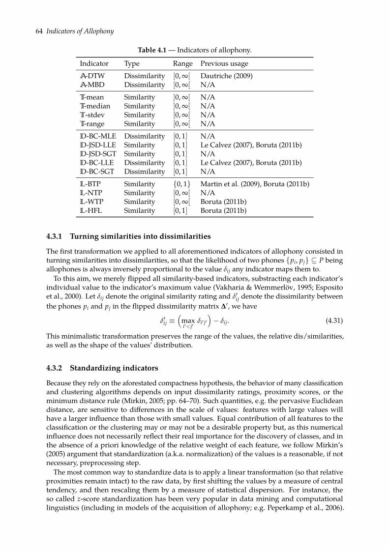
64 Indicators of Allophony
Table 4.1— Indicators of allophony.
Indicator Type Range Previous usage
A-DTW Dissimilarity [0, ∞[ Dautriche (2009)A-MBD Dissimilarity [0, ∞[ N/A
T-mean Similarity ]0, ∞[ N/AT-median Similarity ]0, ∞[ N/AT-stdev Similarity [0, ∞[ N/AT-range Similarity [0, ∞[ N/A
D-BC-MLE Dissimilarity [0, 1] N/AD-JSD-LLE Similarity [0, 1] Le Calvez (2007), Boruta (2011b)D-JSD-SGT Similarity [0, 1] N/AD-BC-LLE Dissimilarity [0, 1] Le Calvez (2007), Boruta (2011b)D-BC-SGT Dissimilarity [0, 1] N/A
L-BTP Similarity 0, 1 Martin et al. (2009), Boruta (2011b)L-NTP Similarity [0, ∞[ N/AL-WTP Similarity [0, ∞[ Boruta (2011b)L-HFL Similarity [0, 1] Boruta (2011b)
4.3.1 Turning similarities into dissimilarities
The first transformation we applied to all aforementioned indicators of allophony consisted inturning similarities into dissimilarities, so that the likelihood of two phones pi, pj ⊆ P beingallophones is always inversely proportional to the value δij any indicator maps them to.To this aim, we merely flipped all similarity-based indicators, substracting each indicator’s
individual value to the indicator’s maximum value (Vakharia & Wemmerlöv, 1995; Espositoet al., 2000). Let δij denote the original similarity rating and δ′ij denote the dissimilarity betweenthe phones pi and pj in the flipped dissimilarity matrix ∆′, we have
δ′ij ≡(
maxi′<j′
δi′ j′)− δij. (4.31)
This minimalistic transformation preserves the range of the values, the relative dis/similarities,as well as the shape of the values’ distribution.
4.3.2 Standardizing indicators
Because they rely on the aforestated compactness hypothesis, the behavior of many classificationand clustering algorithms depends on input dissimilarity ratings, proximity scores, or theminimum distance rule (Mirkin, 2005; pp. 64–70). Such quantities, e.g. the pervasive Euclideandistance, are sensitive to differences in the scale of values: features with large values willhave a larger influence than those with small values. Equal contribution of all features to theclassification or the clustering may or may not be a desirable property but, as this numericalinfluence does not necessarily reflect their real importance for the discovery of classes, and inthe absence of a priori knowledge of the relative weight of each feature, we follow Mirkin’s(2005) argument that standardization (a.k.a. normalization) of the values is a reasonable, if notnecessary, preprocessing step.
The most common way to standardize data is to apply a linear transformation (so that relativeproximities remain intact) to the raw data, by first shifting the values by a measure of centraltendency, and then rescaling them by a measure of statistical dispersion. For instance, theso called z-score standardization has been very popular in data mining and computationallinguistics (including in models of the acquisition of allophony; e.g. Peperkamp et al., 2006).
Numerical recipes 65
It relies on shifting the values by their arithmetic mean and rescaling them by their standarddeviation; yet, as argued by Mirkin (2005; p. 65):
Thus standardized, contributions of all features to data scatter become equal to each otherbecause of the proportionality of contributions and standard deviations. [However], bystandardizing with standard deviations, we deliberately bias data in favor of unimodaldistributions, although obviously it is the bimodal distribution that should contribute toclustering most.~
This observation is especially true in the case at hand, where features are the aforementionedindicators of allophony. Indeed, as stated in Section 4.1.2, our goal is to discover bimodaldistributions in the input data, distributions whose modes emblematize the dichotomy betweenallophonic and non-allophonic pairs of phones.
Range standardization In order to circumvent the limitations inherent to the use of standarddeviation as the scaling factor, Mirkin (2005) recommends using the values’ range as an appro-priate scaling factor. Hence, the first standardization technique we consider in the present studyconsists in first shifting by the minimum value and then rescaling by the range. Let δ′ij denotethe dissimilarity between the phones pi and pj in the range-standardized dissimilarity matrix ∆′,we have
δ′ij ≡δij − (mini′<j′ δi′ j′)
(maxi′<j′ δi′ j′)− (mini′<j′ δi′ j′). (4.32)
Using this standardization technique, both relative dissimilarities and the shape of the distribu-tions are preserved, but all values lie in the same range, i.e. [0, 1].
Ranks standardization Because of the assumptions underlying Peperkamp et al.’s (2006) frame-work, we introduce another standardization technique that we will refer to as rank standard-ization. All things considered, the main assumption behind what we refer to as indicators ofallophony is indeed that allophonic pairs should be more similar than non-allophonic pairs. Putanother way, allophonic pairs should rank lower than non-allophonic pairs in the arrangementof all phone pairs pi, pj ⊆ P by increasing order of the values to which a given indicator mapsthem. Thus, a transversal problem (that we address is this chapter and the next) is to determinewhether allophony and phonemehood can be learned by amere ranking of the candidate pairs, orif the actual dissimilarity ratings denoted by each indicator’s values are meaningful. To this aim,we will compare the results obtained with both range- and ranks-based standardizations. Let δ′ijdenote the dissimilarity between the phones pi and pj in the ranks-standardized dissimilaritymatrix ∆′. In the general case, we have
δ′ij ≡ 1 +∣∣pi′ , pj′ ⊆ P : δi′ j′ < δij
∣∣ , (4.33)that is to say the rank of the pair pi, pj is given by 1 plus the number of pairs with stricly lesservalues. In the case of tied values, the ranks of the corresponding pairs are averaged (Jones et al.,2001; cf. scipy.stats.mstats.rankdata); for example, if the minimal value a given indicatorcan take is attested for two distinct phone pairs, both pairs would receive the pseudorank of(1 + 2)/2 = 1.5.
4.3.3 Addressing the frequency effect
As highlighted in Sections 3.1.3 and 3.2, various frequency effects can be observed in our data:on one hand, the distribution of phoneme frequencies follows a power law (cf. Figure 3.2) and,on the other hand, the number of allophones HTK computes for a given phoneme appears to be,at any allophonic complexity, positively correlated with that phoneme’s frequency (cf. Table 3.7).However, having equal expectations for the performance of a computational model on the
least and the most frequent instances of the problem would be unrealistic. Indeed, trainingany such model on the CSJ implies examining 50 times less evidence for the allophones of /i:/
66 Indicators of Allophony
than for the allophones of /a/. Notwithstanding potential sampling issues in the constitution ofthe CSJ, we consider this lack of balance in our data to be an inherent property of the Japaneselanguage; yet, we will account for this imbalance by assigning a frequency-based weight to eachphone pair pi, pj in the allophonic inventory P.
Individual weights The weighting scheme we introduce in the present study relies on merefrequency counts. Concretely, for a given allophonic inventory P, the weight wi ∈N we assignto each phone pi ∈ P is given the frequency of occurrence of pi in the corpus, i.e. wi ≡ #(pi) (cf.Section 4.2.3). As all allophones were computed by HTK on the basis of the actual content of theCSJ (rather than using an a priori allophonic grammar of Japanese), all individual weights are,by definition, strictly positive. As a matter of convenience, let w denote the vector of length ncollecting all individual weights, i.e. w ≡ (w1, . . . , wn).Because such weights are estimated by the phones’ occurrence frequencies, they can be inter-
preted as instance weights. Repeating our prior analogy with canopy clustering (McCallum et al.,2000), any allophonic inventory can be considered as the output of a canopy clustering techniquewhereby the inherent variability in human speech was reduced to a finite, quantized set of objects(i.e. the allophones) complemented with information about the fraction of variability accountedfor by each canopy (i.e. the phones and their respective weights, the latter indicating how manysound tokens were used to estimate the parameters of each allophonic HMM).Compared to previous studies building upon Peperkamp et al.’s (2006) and, especially, those
where a systematic examination of the influence of the input’s allophonic complexity wasconducted (Martin et al., 2009; Boruta, 2009, 2011b), using frequency-based instance weights willfacilitate the comparability between a given model’s outputs at various complexities. Indeed,another consequence of using frequency-based instance weights is that the total number ofinstances (i.e. ∑i wi) is constant across all possible allophonic complexities, as it is equal to theoverall number of sound tokens in the input corpus.
Pairwiseweights In Peperkamp et al.’s framework, the core object to bemanipulated is a pair ofphones. Therefore, we propose the following straightforward extension of our frequency-baseddefinition of weights to phone pairs. We define the weight wij ∈N assigned to the phone pairpi, pj ⊆ P as the product of both phones’ individual weights, i.e. wij ≡ wiwj. As a matter ofconvenience, let W denote the symmetric n× n weight matrix W ≡ [wij] in which all pairwiseweights are collected.
Because the individual weight wi is given by the number of sound tokens that were canopy-clustered as the phone pi, the pairwise weight wij ≡ wiwj can also be interpreted as an instanceweight: indeed, wij is equal to the number of sound pairs in which one sound token was canopy-clustered as pi and the other as pj. For each tested allophonic complexity, the distribution of thepairwise weights is illustrated in Figure 4.4, using a logarithmic scale to account for the greatvariability between weights computed for pairs consisting in two high-frequency phones and forpairs consisting in two low-frequency phones. The box plots in Figure 4.4 suggest that, whereasthe median pairwise weight decreases as the allophonic complexity increases, pairwise weights’attested range enlarges until it plateaus, from 782/25 allophone per phoneme onwards.
There’s no such thing as a free lunch As far as allophony is concerned, the introduction ofpairwise weights in the framework has one major consequence: it alters the ratio of the numberof allophonic pairs to the number of non-allophonic pairs. In order to quantify the influence ofpairwise weights on class balance, we computed two such ratios. On one hand, we computed theallophonic to non-allophonic ratio as would be observed by Peperkamp et al.’s (2006) learner, i.e.
class-balance(A∗) ≡∑i<jJa∗ij = 1K
∑i<jJa∗ij = 0K, (4.34)
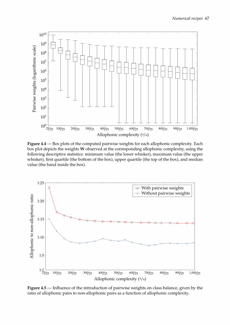
Numerical recipes 67
100/25 200/25 300/25 400/25 500/25 600/25 700/25 800/25 900/25 1,000/25100
101
102
103
104
105
106
107
108
109
1010
25/25
Allophonic complexity (n/n)
Pair
wis
ew
eigh
ts(lo
garit
hmic
scal
e)
Figure 4.4 — Box plots of the computed pairwise weights for each allophonic complexity. Eachbox plot depicts the weights W observed at the corresponding allophonic complexity, using thefollowing descriptive statistics: minimum value (the lower whisker), maximum value (the upperwhisker), first quartile (the bottom of the box), upper quartile (the top of the box), and medianvalue (the band inside the box).
100/25 200/25 300/25 400/25 500/25 600/25 700/25 800/25 900/25 1,000/25
1:5
1:10
1:15
1:20
1:25
25/251:1
Allophonic complexity (n/n)
Allo
phon
icto
non-
allo
phon
icra
tio
With pairwise weightsWithout pairwise weights
Figure 4.5 — Influence of the introduction of pairwise weights on class balance, given by theratio of allophonic pairs to non-allophonic pairs as a function of allophonic complexity.
68 Indicators of Allophony
and, on the other hand, we computed the updated allophonic to non-allophonic ratio, as will beobserved by our learner—that is to say, when pairwise weights are available, i.e.
class-balance(A∗, W) ≡∑i<j wijJa∗ij = 1K
∑i<j wijJa∗ij = 0K. (4.35)
The results are presented in Figure 4.5 as a function of the allophonic complexity of the testedinventories. Notwithstanding the lowest allophonic complexities such as 48/25 or 98/25 allophonesper phoneme, these ratios appear to be quite unchanging: while, broady speaking, not usingfrequency information yields a ratio of the number of allophonic pairs to the number of non-allophonic pairs approximately equal to 1:8, using frequency-based pairwise weights yields aratio approximately equal to 1:14.As will be further discussed in Chapter 5, one limitation of Peperkamp et al.’s framework is
that the learner has to process all possible phone pairs to discover which ones are allophones. Inthe case at hand, non-allophonic pairs are therefore useless, as no relation brings such phonestogether. Therefore, whereas an artificial learner à la Peperkamp et al. has to reject, on average,7 out of every 8 phone pairs, an artificial learner provided with frequency information wouldhave to reject 13 out of every 14 phone pairs. Hence, accounting for the power law in phonemefrequencies comes at the cost of increasing the proportion of negative objects in the input data,hence the title of this paragraph.
4.4 Prognoses of allophony
This section contains a preliminary examination of indicators’ performance for the discriminationof allophonic pairs vs. non-allophonic pairs. This examination is actually twofold. First, wereplicate part of Martin et al.’s (2009) experiments using a probabilistic assessment of classseparation that quantifies, for a given indicator of allophony, the probability of non-allophonicpairs being more dissimilar than allophonic pairs. Second, we introduce a novel visualizationtechnique allowing for the exploration of the classwise distribution of an indicator’s values.Our focus here is on emphasizing the distinction between such tools, that we refer to as
prognoses, and true evaluation methods. Whereas the purpose of an evaluation method isto judge the output of a given model or algorithm on a given task according to given qualitycriteria, the purpose of a prognosis method is to inspect the data in order to provide a betterunderstanding of its inner content and structure, and to hint at transformations or algorithmsthat would be relevant for the task at hand. In other words, a prognosis method does not suggestconclusions: it supports decision making and, at best, it suggests expectations.
4.4.1 Rank-sum test of class separation
The first prognosis of allophony we present is a rank-sum test, originally proposed by Herrnsteinet al. (1976), and first used in the context of allophony learning by Martin et al. (2009). Giventwo observation samples, this non-parametric test aims at assessing whether one of the twosamples tends to have larger values than the other. In the case at hand, we test the hypothesisthat non-allophonic pairs tend to be more dissimilar than allophonic pairs.
Definitions Herrnstein et al.’s (1976) statistic, denoted ρ, is equal to the probability of non-allophonic pairs being more dissimilar than allophonic pairs. Let A∗ and ∆ denote, respectively,the reference allophony matrix and the dissimilarity matrix collecting the values of a givenindicator of allophony. Concretely, ρ is a MLE of the probability that a randomly-drawn non-allophonic pair will score higher than a randomly-drawn allophonic pair in ∆. We first give adefinition of ρ without taking instance weights into account, i.e. as used by Martin et al. (2009).
Prognoses of allophony 69
In this case, we have
ρ(∆; A∗) ≡∑i<j ∑i′<j′Ja∗ij = 0KJa∗i′ j′ = 1KJδij > δi′ j′K(
∑i<jJa∗ij = 0K)(
∑i′<j′Ja∗i′ j′ = 1K) . (4.36)
To our knowledge, no formulation of ρ has been proposed so far to account for weighted obser-vation samples. Using the frequency-based instance weights collected in W, as defined in theprevious section, we propose the following weighted extension of the definition of ρ:
ρ(∆; A∗, W) ≡∑i<j ∑i′<j′ wijwi′ j′Ja∗ij = 0KJa∗i′ j′ = 1KJδij > δi′ j′K(
∑i<j wijJa∗ij = 0K)(
∑i′<j′ wi′ j′Ja∗i′ j′ = 1K) . (4.37)
This amended definition is consistent with our conception of weights as instance weights: wiwas defined as the number of sound tokens that were canopy-clustered as pi, wij ≡ wiwj wasdefined as the number of pairs of sound tokens in which one sound was canopy-clustered as piand the other as pj, and the product wijwi′ j′ in the numerator of Equation 4.37 is equal to thenumber of pairs of pairs of sound tokens in which the first pair was canopy-clustered as pi, pjand the other as pi′ , pj′.
It is worth mentioning that these definitions of ρ with a double summation are given here forthe sake of simplicity: a straightforward implementation of these definitions would howeverrequireO(n4) operations, as it would consist in iterating over all possible pairs of pairs of phones;yet, becauseHerrnstein et al.’s test relies on ranks, the time complexity of the computation of ρ canbe reduced to O(n2 log2 n) by first copying all pairwise dissimilarity ratings (the lower trianglein ∆) into a list, sorting this list—hence the linearithmic complexity—and then working on theranks of the values in the sorted list (Jones et al., 2001; cf. scipy.stats.mstats.mannwhitneyu).Being probability estimates, all ρ values (weighted or not) lie in [0, 1] and ρ = .5 indicates
chance. Whereas high and low values both indicate a significant separation of the two allophonicstatuses in ∆, it is worth noting that values strictly below .5 indicate a reverse separation ofstatuses; in that case, allophonic pairs tend to be mapped to larger dissimilarity ratings thannon-allophonic pairs and, thus, the indicator is in fact a similarity measure. While indicatorswith ρ < .5 could be turned into proper indicators of allophony by flipping their values (cf.Section 4.3.1), indicators with ρ = .5 simply contain no relevant information for the purpose ofseparating allophonic pairs from non-allophonic ones. For instance, a uniform, random drawingof dissimilarity ratings would yield a ρ value equal to .5.
Chances of allophony Herrnstein et al.’s rank-sum test is related to other statistics, viz. thearea under the receiver operating characteristic curve (a.k.a. the AUC) and the Mann–Whitney Utest. All these statistics, however, should not be considered as appropriate evaluation measuresin the case at hand, as they do not rely on a partition of all possible phone pairs into allophonicand non-allophonic pairs. Indeed, although we ambiguously argued in a previous study thatρ may be used to evaluate the performance of an indicator across all possible discriminationthresholds (Boruta, 2011b; p. 2), its limitation lies in the fact that no explicit discriminationthreshold is actually applied or even searched for. For this reason, ρ is nothing but a prognosisof allophony: it is a probabilistic assessment of how effective a given indicator may be, not acomplete algorithm that decides which pairs of phones are allophones and which are not.
Results Weighted ρ values are presented in Figures 4.6, 4.7, 4.8, and 4.9 as a function ofallophonic complexity for acoustic, temporal, distributional, and lexical indicators, respectively.Let us mention immediately that, throughout the present study, the y-axes of all plots illustratingprognoses or evaluation measures are annotated with an arrow indicating how the particularmeasure should be interpreted: ↑ for measures that are positively correlated with the quality ofthe underlying data (i.e. the higher the better), and ↓ for measures that are inversely correlatedwith the quality of the underlying data (the lower the better).
As presented in Figure 4.6, the prognosis of class separation for acoustic indicators is encour-aging. First and foremost, both acoustic indicators’ prognosis of allophony is significantly above
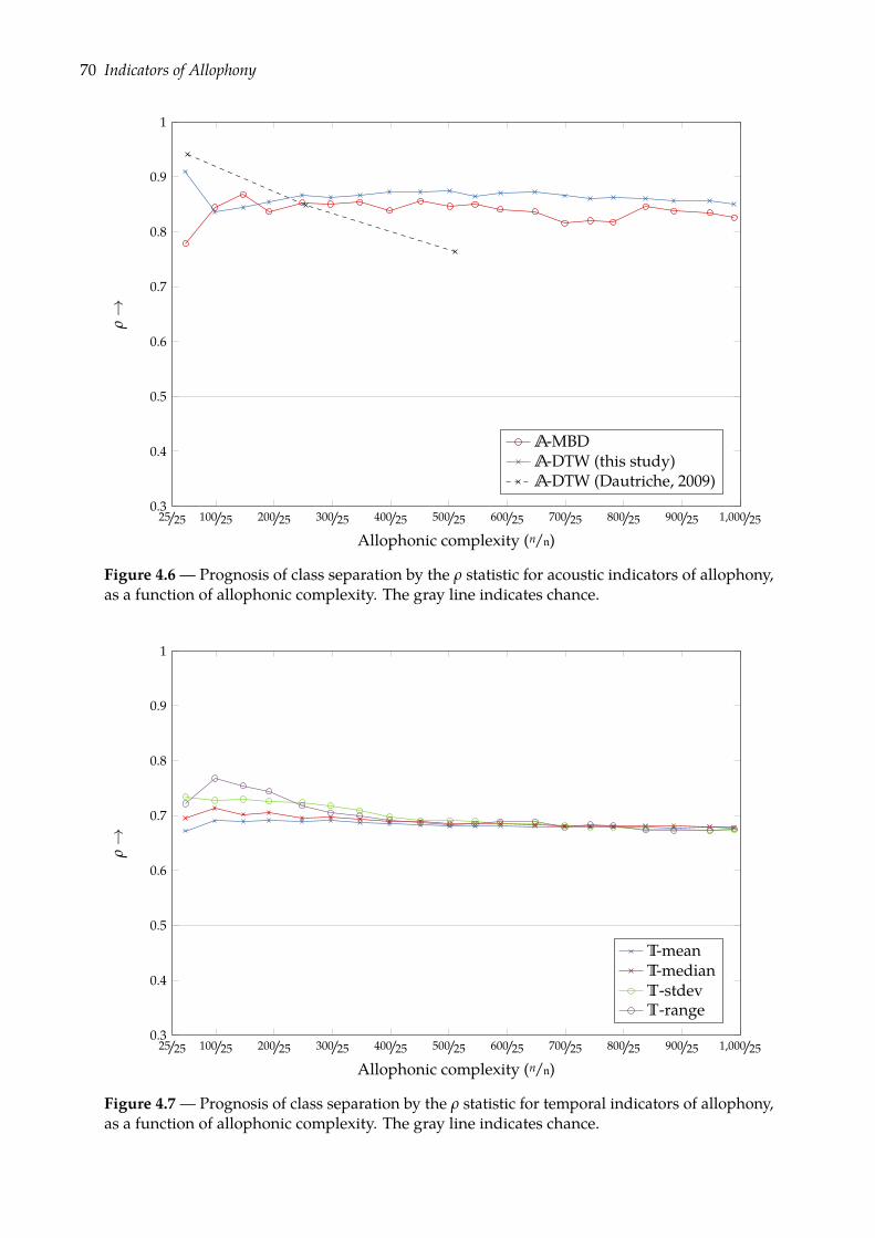
70 Indicators of Allophony
100/25 200/25 300/25 400/25 500/25 600/25 700/25 800/25 900/25 1,000/250.3
0.4
0.5
0.6
0.7
0.8
0.9
1
25/25
Allophonic complexity (n/n)
ρ→
A-MBDA-DTW (this study)A-DTW (Dautriche, 2009)
Figure 4.6 — Prognosis of class separation by the ρ statistic for acoustic indicators of allophony,as a function of allophonic complexity. The gray line indicates chance.
100/25 200/25 300/25 400/25 500/25 600/25 700/25 800/25 900/25 1,000/250.3
0.4
0.5
0.6
0.7
0.8
0.9
1
25/25
Allophonic complexity (n/n)
ρ→
T-meanT-medianT-stdevT-range
Figure 4.7 — Prognosis of class separation by the ρ statistic for temporal indicators of allophony,as a function of allophonic complexity. The gray line indicates chance.
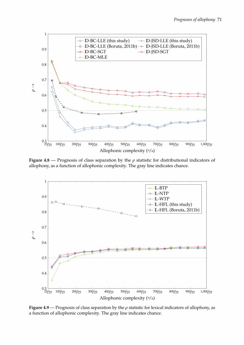
Prognoses of allophony 71
100/25 200/25 300/25 400/25 500/25 600/25 700/25 800/25 900/25 1,000/250.3
0.4
0.5
0.6
0.7
0.8
0.9
1
25/25
Allophonic complexity (n/n)
ρ→
D-BC-LLE (this study) D-JSD-LLE (this study)D-BC-LLE (Boruta, 2011b) D-JSD-LLE (Boruta, 2011b)D-BC-SGT D-JSD-SGTD-BC-MLE
Figure 4.8 — Prognosis of class separation by the ρ statistic for distributional indicators ofallophony, as a function of allophonic complexity. The gray line indicates chance.
100/25 200/25 300/25 400/25 500/25 600/25 700/25 800/25 900/25 1,000/250.3
0.4
0.5
0.6
0.7
0.8
0.9
1
25/25
Allophonic complexity (n/n)
ρ→
L-BTPL-NTPL-WTPL-HFL (this study)L-HFL (Boruta, 2011b)
Figure 4.9— Prognosis of class separation by the ρ statistic for lexical indicators of allophony, asa function of allophonic complexity. The gray line indicates chance.
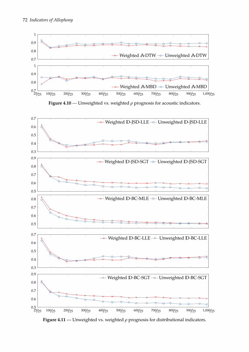
72 Indicators of Allophony
0.7
0.8
0.9
1
Weighted A-DTW Unweighted A-DTW
100/25 200/25 300/25 400/25 500/25 600/25 700/25 800/25 900/25 1,000/250.7
0.8
0.9
1
25/25
Weighted A-MBD Unweighted A-MBD
Figure 4.10—Unweighted vs. weighted ρ prognosis for acoustic indicators.
0.3
0.4
0.5
0.6
0.7Weighted D-JSD-LLE Unweighted D-JSD-LLE
0.5
0.6
0.7
0.8
0.9Weighted D-JSD-SGT Unweighted D-JSD-SGT
0.5
0.6
0.7
0.8 Weighted D-BC-MLE Unweighted D-BC-MLE
0.3
0.4
0.5
0.6
0.7Weighted D-BC-LLE Unweighted D-BC-LLE
100/25 200/25 300/25 400/25 500/25 600/25 700/25 800/25 900/25 1,000/250.5
0.6
0.7
0.8
0.9
25/25
Weighted D-BC-SGT Unweighted D-BC-SGT
Figure 4.11 —Unweighted vs. weighted ρ prognosis for distributional indicators.
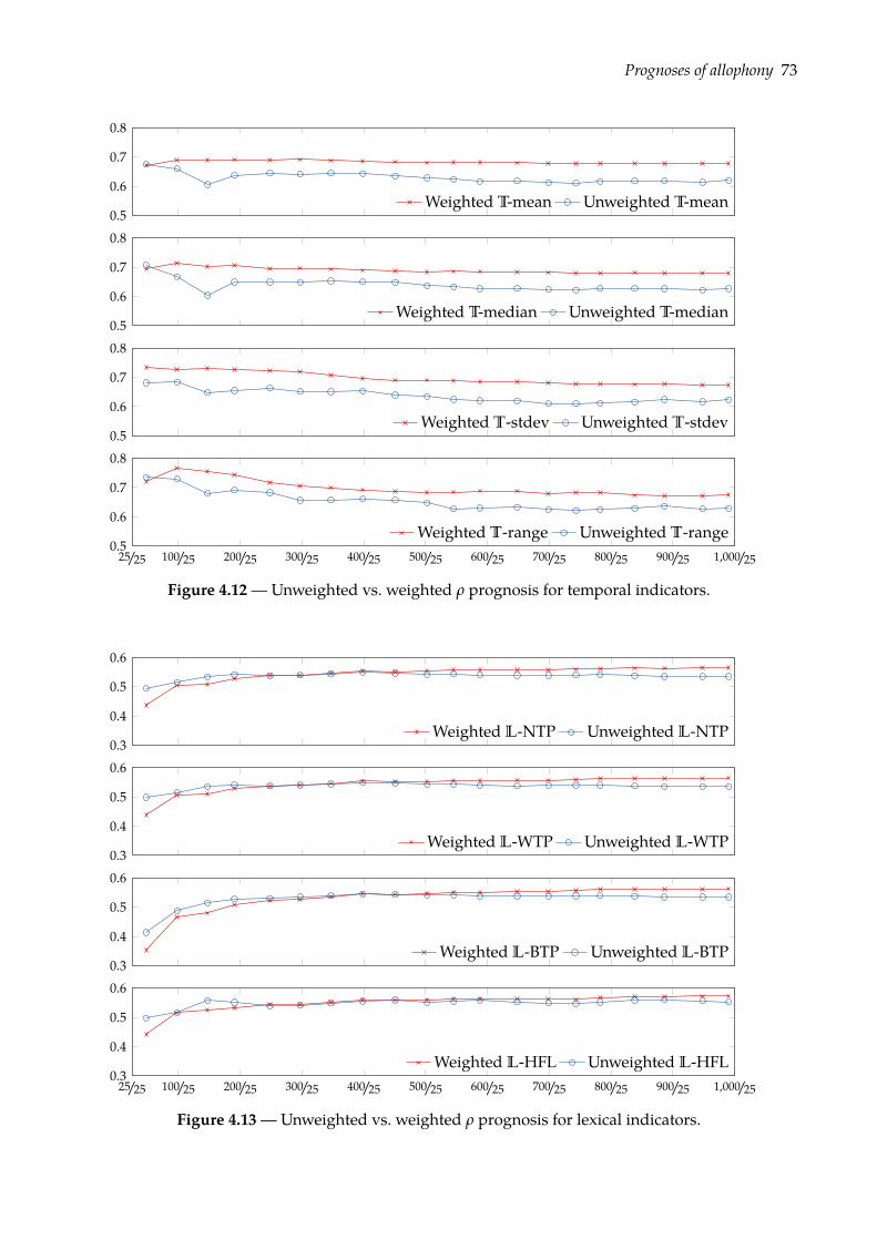
Prognoses of allophony 73
0.5
0.6
0.7
0.8
Weighted T-mean Unweighted T-mean
0.5
0.6
0.7
0.8
Weighted T-median Unweighted T-median
0.5
0.6
0.7
0.8
Weighted T-stdev Unweighted T-stdev
100/25 200/25 300/25 400/25 500/25 600/25 700/25 800/25 900/25 1,000/250.5
0.6
0.7
0.8
25/25
Weighted T-range Unweighted T-range
Figure 4.12 —Unweighted vs. weighted ρ prognosis for temporal indicators.
0.3
0.4
0.5
0.6
Weighted L-NTP Unweighted L-NTP
0.3
0.4
0.5
0.6
Weighted L-WTP Unweighted L-WTP
0.3
0.4
0.5
0.6
Weighted L-BTP Unweighted L-BTP
100/25 200/25 300/25 400/25 500/25 600/25 700/25 800/25 900/25 1,000/250.3
0.4
0.5
0.6
25/25
Weighted L-HFL Unweighted L-HFL
Figure 4.13 —Unweighted vs. weighted ρ prognosis for lexical indicators.
74 Indicators of Allophony
chance. Moreover, A-DTW and A-MBD seem to be resistant (if not insensitive) to an increasein allophonic complexity. Indeed, as the complexity of the input increases, ρ values tend tolie in the [.8, .9] band, indicating that there is more than 8 chances in 10 of a randomly-drawnnon-allophonic pair being acoustically more dissimilar than a randomly-drawn allophonic pair.Therefore, despite the fact that allophones were computed by HTK on the basis of the acousticdissimilarity between their realizations, it appears that any given phoneme’s allophones are still,on average, acoustically homogeneous. Because they were derived from a comparable corpus—viz. the CSJ, albeit using unmatchable preprocessing choices—we also report in Figure 4.6 the ρvalues obtained by Dautriche (2009) for A-DTW. These three points suffice to suggest that, inthat setup, A-DTW does not resist an increase in allophonic complexity. Because both studiesrely on the identical definitions of A-DTW, this discrepancy is necessarily due to Dautriche’stranscription scheme. Indeed, in that study, allophonic HMMswere trained for an inventory of 49phonemic categories in which, for example, allophonic palatalizations were kept transcribed as-is.We suspect that, because of this subphonemic transcription scheme, Dautriche’s experiments raninto the data sparseness problem we circumvented in Section 3.1: all other things being equal,doubling the number of phoneme-level categories can only scatter the information available inthe training corpus.
Although less impressive than that of the acoustic indicators, the prognosis of class separationfor temporal indicators is surprisingly good, especially considering the limited information onwhich these indicators rely. As presented in Figure 4.7, all four indicators’ ρ values tend to ρ ≈ .7as the allophonic complexity of their input increases. Indeed, T-mean, T-median, T-stdev, andT-range hardly suffer an increase in allophonic complexity and are virtually indistinguishablefrom 450/25 allophones per phoneme onwards. Not only do these indicators of allophony sharethe same underlying logic, they also appear to share the same behavior, regardless of the exactdefinition of their ancillary statistic and, more surprisingly, no matter whether the focus is oncomparing the central tendency or the statistical dispersion of both phones’ durations. It is worthnoting, however, that indicators relying on measures of statistical dispersion yield a slightlybetter separation of allophonic statuses at lower allophonic complexities.While the behavior of both acoustic and temporal indicators of allophony looks promising,
the same cannot be said for distributional indicators, as presented in Figure 4.8. Indeed, all fiveindicators’ prognoses drop significantly for the first increases in allophonic complexity. Martinet al. (2009) argued that this is due to the fact that, in corpora of high allophonic complexity,every phone has an extremely narrow distribution and, hence, having complementary (or, tosay the least, dissimilar) distributions is the rule rather than the exception. Notwithstandingthis sensitivity to allophonic complexity, the major observation is that while the very definitionof the measure used to compare both phones’ context distributions (viz. JSD or BC) appear tohave virtually no effect on the prognosis of class separation, the technique used to estimatethe probabilities has a significant impact. Indeed, three groups emerge in Figure 4.8: theindicators relying on SGT estimates whose ρ tend to values slightly above .6, the indicatorrelying on MLEs whose ρ tend to chance, and the indicators relying on LLEs whose ρ dropsbelow chance from 98/25 allophones per phoneme onwards. This last observation corroboratespreviously reported ρ values for distributional indicators relying on LLEs (Martin et al., 2009;Boruta, 2011b); yet, whereas we previously observed (Boruta, 2011b) that the prognosis of classseparation for indicators relying on LLEs of SKLD, JSD, or BC indeed drops below chance asthe complexity of their input increases (as reported in Figure 4.8 for comparable indicators),Martin et al.’s (2009) figures suggest that their SKLD-based indicator plateaus slightly abovechance. We are unfortunately unable to account for this discrepancy except, maybe, by an effectof the very different processes used to create the allophonic inventories (linguistic rules vs.random partitions, as presented in Section 3.2.1). Furthermore, while assessing the numericaldiscrepancies between LLE- and SGT-based smoothing would be intractable—as it amounts tothe examination of thousands of probability distributions—this shallow comparison is sufficientto show that Peperkamp et al.’s (2006) use of smoothing as a numerical recipe to avoid null
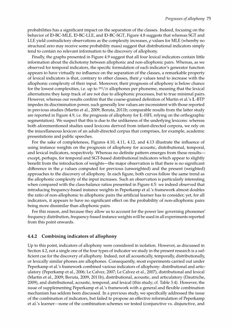
Prognoses of allophony 75
probabilities has a significant impact on the separation of the classes. Indeed, focusing on thebehavior of D-BC-MLE, D-BC-LLE, and D-BC-SGT, Figure 4.8 suggests that whereas SGT andLLE yield contradictory observations as the complexity increases, ρ values for MLE (whereby nostructural zero may receive some probability mass) suggest that distributional indicators simplytend to contain no relevant information to the discovery of allophony.
Finally, the graphs presented in Figure 4.9 suggest that all four lexical indicators contain littleinformation about the dichotomy between allophonic and non-allophonic pairs. Whereas, as weobserved for temporal indicators, the specific formulation of each indicator’s generator functionappears to have virtually no influence on the separation of the classes, a remarkable propertyof lexical indicators is that, contrary to other classes, their ρ values tend to increase with theallophonic complexity of their input. Moreover, their prognosis of allophony is below chancefor the lowest complexities, i.e. up to 191/25 allophones per phoneme, meaning that the lexicalalternations they keep track of are not due to allophonic processes, but to true minimal pairs.However, whereas our results confirm that the coarse-grained definition of Martin et al.’s L-BTPimpedes its discrimination power, such generally low values are inconsistent with those reportedin previous studies (Martin et al., 2009; Boruta, 2011b; comparable results from the latter studyare reported in Figure 4.9, i.e. the prognosis of allophony for L-HFL relying on the orthographicsegmentation). We suspect that this is due to the unlikeness of the underlying lexicons: whereasboth aforementioned studies used lexicons derived from infant-directed corpora, we rely onthe miscellaneous lexicon of an adult-directed corpus that comprises, for example, academicpresentations and public speeches.
For the sake of completeness, Figures 4.10, 4.11, 4.12, and 4.13 illustrate the influence ofusing instance weights on the prognosis of allophony for acoustic, distributional, temporal,and lexical indicators, respectively. Whereas no definite pattern emerges from these results—except, perhaps, for temporal and SGT-based distributional indicators which appear to slightlybenefit from the introduction of weights—the major observation is that there is no significantdifference in the ρ values computed for previous (unweighted) and the present (weighted)approaches to the discovery of allophony. In each figure, both curves follow the same trend asthe allophonic complexity of the input increases. Such an observation is particularly interestingwhen compared with the class-balance ratios presented in Figure 4.5: we indeed observed thatintroducing frequency-based instance weights in Peperkamp et al.’s framework almost doublesthe ratio of non-allophonic to allophonic pairs the artificial learner has to consider; yet, for allindicators, it appears to have no significant effect on the probability of non-allophonic pairsbeing more dissimilar than allophonic pairs.
For this reason, and because they allow us to account for the power law governing phonemes’frequency distribution, frequency-based instanceweightswill be used in all experiments reportedfrom this point onwards.
4.4.2 Combining indicators of allophony
Up to this point, indicators of allophony were considered in isolation. However, as discussed inSection 4.2, not a single one of the four types of indicator we study in the present research is a suf-ficient cue for the discovery of allophony. Indeed, not all acoustically, temporally, distributionally,or lexically similar phones are allophones. Consequently, most experiments carried out underPeperkamp et al.’s framework combined various indicators of allophony: distributional and artic-ulatory (Peperkamp et al., 2006; Le Calvez, 2007; Le Calvez et al., 2007), distributional and lexical(Martin et al., 2009; Boruta, 2009, 2011b), distributional, acoustic, and articulatory (Dautriche,2009), and distributional, acoustic, temporal, and lexical (this study; cf. Table 3.4). However, theissue of supplementing Peperkamp et al.’s framework with a general and flexible combinationmechanism has seldom been discussed. In a previous study, we specifically addressed the issueof the combination of indicators, but failed to propose an effective reformulation of Peperkampet al.’s learner—none of the combination schemes we tested (conjunctive vs. disjunctive, and
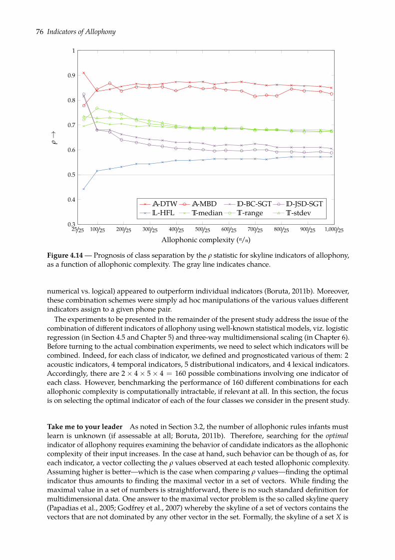
76 Indicators of Allophony
100/25 200/25 300/25 400/25 500/25 600/25 700/25 800/25 900/25 1,000/250.3
0.4
0.5
0.6
0.7
0.8
0.9
1
25/25
Allophonic complexity (n/n)
ρ→
A-DTW A-MBD D-BC-SGT D-JSD-SGTL-HFL T-median T-range T-stdev
Figure 4.14 — Prognosis of class separation by the ρ statistic for skyline indicators of allophony,as a function of allophonic complexity. The gray line indicates chance.
numerical vs. logical) appeared to outperform individual indicators (Boruta, 2011b). Moreover,these combination schemes were simply ad hoc manipulations of the various values differentindicators assign to a given phone pair.
The experiments to be presented in the remainder of the present study address the issue of thecombination of different indicators of allophony using well-known statistical models, viz. logisticregression (in Section 4.5 and Chapter 5) and three-way multidimensional scaling (in Chapter 6).Before turning to the actual combination experiments, we need to select which indicators will becombined. Indeed, for each class of indicator, we defined and prognosticated various of them: 2acoustic indicators, 4 temporal indicators, 5 distributional indicators, and 4 lexical indicators.Accordingly, there are 2× 4× 5× 4 = 160 possible combinations involving one indicator ofeach class. However, benchmarking the performance of 160 different combinations for eachallophonic complexity is computationally intractable, if relevant at all. In this section, the focusis on selecting the optimal indicator of each of the four classes we consider in the present study.
Take me to your leader As noted in Section 3.2, the number of allophonic rules infants mustlearn is unknown (if assessable at all; Boruta, 2011b). Therefore, searching for the optimalindicator of allophony requires examining the behavior of candidate indicators as the allophoniccomplexity of their input increases. In the case at hand, such behavior can be though of as, foreach indicator, a vector collecting the ρ values observed at each tested allophonic complexity.Assuming higher is better—which is the case when comparing ρ values—finding the optimalindicator thus amounts to finding the maximal vector in a set of vectors. While finding themaximal value in a set of numbers is straightforward, there is no such standard definition formultidimensional data. One answer to the maximal vector problem is the so called skyline query(Papadias et al., 2005; Godfrey et al., 2007) whereby the skyline of a set of vectors contains thevectors that are not dominated by any other vector in the set. Formally, the skyline of a set X is
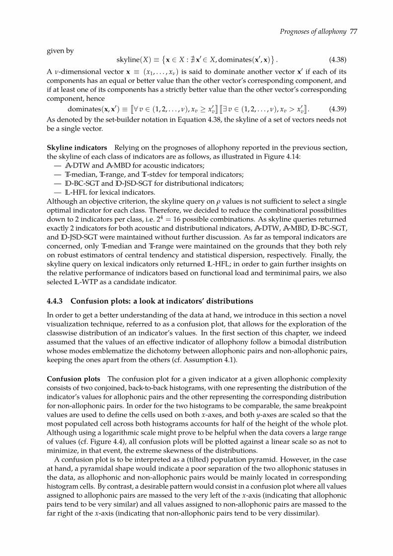
Prognoses of allophony 77
given byskyline(X) ≡
x ∈ X : @ x′∈ X, dominates(x′, x)
. (4.38)
A ν-dimensional vector x ≡ (x1, . . . , xν) is said to dominate another vector x′ if each of itscomponents has an equal or better value than the other vector’s corresponding component, andif at least one of its components has a strictly better value than the other vector’s correspondingcomponent, hence
dominates(x, x′) ≡q∀ v ∈ (1, 2, . . . , ν), xv ≥ x′v
yq∃ v ∈ (1, 2, . . . , ν), xv > x′v
y. (4.39)
As denoted by the set-builder notation in Equation 4.38, the skyline of a set of vectors needs notbe a single vector.
Skyline indicators Relying on the prognoses of allophony reported in the previous section,the skyline of each class of indicators are as follows, as illustrated in Figure 4.14:— A-DTW and A-MBD for acoustic indicators;— T-median, T-range, and T-stdev for temporal indicators;— D-BC-SGT and D-JSD-SGT for distributional indicators;— L-HFL for lexical indicators.
Although an objective criterion, the skyline query on ρ values is not sufficient to select a singleoptimal indicator for each class. Therefore, we decided to reduce the combinatioral possibilitiesdown to 2 indicators per class, i.e. 24 = 16 possible combinations. As skyline queries returnedexactly 2 indicators for both acoustic and distributional indicators, A-DTW, A-MBD, D-BC-SGT,and D-JSD-SGT were maintained without further discussion. As far as temporal indicators areconcerned, only T-median and T-range were maintained on the grounds that they both relyon robust estimators of central tendency and statistical dispersion, respectively. Finally, theskyline query on lexical indicators only returned L-HFL; in order to gain further insights onthe relative performance of indicators based on functional load and terminimal pairs, we alsoselected L-WTP as a candidate indicator.
4.4.3 Confusion plots: a look at indicators’ distributions
In order to get a better understanding of the data at hand, we introduce in this section a novelvisualization technique, referred to as a confusion plot, that allows for the exploration of theclasswise distribution of an indicator’s values. In the first section of this chapter, we indeedassumed that the values of an effective indicator of allophony follow a bimodal distributionwhose modes emblematize the dichotomy between allophonic pairs and non-allophonic pairs,keeping the ones apart from the others (cf. Assumption 4.1).
Confusion plots The confusion plot for a given indicator at a given allophonic complexityconsists of two conjoined, back-to-back histograms, with one representing the distribution of theindicator’s values for allophonic pairs and the other representing the corresponding distributionfor non-allophonic pairs. In order for the two histograms to be comparable, the same breakpointvalues are used to define the cells used on both x-axes, and both y-axes are scaled so that themost populated cell across both histograms accounts for half of the height of the whole plot.Although using a logarithmic scale might prove to be helpful when the data covers a large rangeof values (cf. Figure 4.4), all confusion plots will be plotted against a linear scale so as not tominimize, in that event, the extreme skewness of the distributions.A confusion plot is to be interpreted as a (tilted) population pyramid. However, in the case
at hand, a pyramidal shape would indicate a poor separation of the two allophonic statuses inthe data, as allophonic and non-allophonic pairs would be mainly located in correspondinghistogram cells. By contrast, a desirable patternwould consist in a confusion plot where all valuesassigned to allophonic pairs are massed to the very left of the x-axis (indicating that allophonicpairs tend to be very similar) and all values assigned to non-allophonic pairs are massed to thefar right of the x-axis (indicating that non-allophonic pairs tend to be very dissimilar).
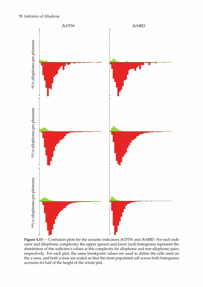
78 Indicators of Allophony
A-DTW A-MBD
48/2
5alloph
ones
perp
hone
me
502 /
25alloph
ones
perp
hone
me
990 /
25alloph
ones
perp
hone
me
Figure 4.15 —Confusion plots for the acoustic indicators A-DTW and A-MBD. For each indi-cator and allophonic complexity, the upper (green) and lower (red) histograms represent thedistribution of this indicator’s values at this complexity for allophonic and non-allophonic pairs,respectively. For each plot, the same breakpoint values are used to define the cells used onthe x-axes, and both y-axes are scaled so that the most populated cell across both histogramsaccounts for half of the height of the whole plot.
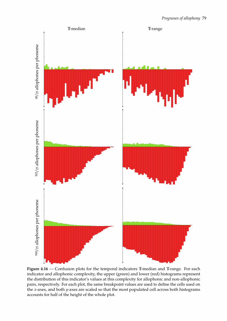
Prognoses of allophony 79
T-median T-range
48/2
5alloph
ones
perp
hone
me
502 /
25alloph
ones
perp
hone
me
990 /
25alloph
ones
perp
hone
me
Figure 4.16 — Confusion plots for the temporal indicators T-median and T-range. For eachindicator and allophonic complexity, the upper (green) and lower (red) histograms representthe distribution of this indicator’s values at this complexity for allophonic and non-allophonicpairs, respectively. For each plot, the same breakpoint values are used to define the cells used onthe x-axes, and both y-axes are scaled so that the most populated cell across both histogramsaccounts for half of the height of the whole plot.
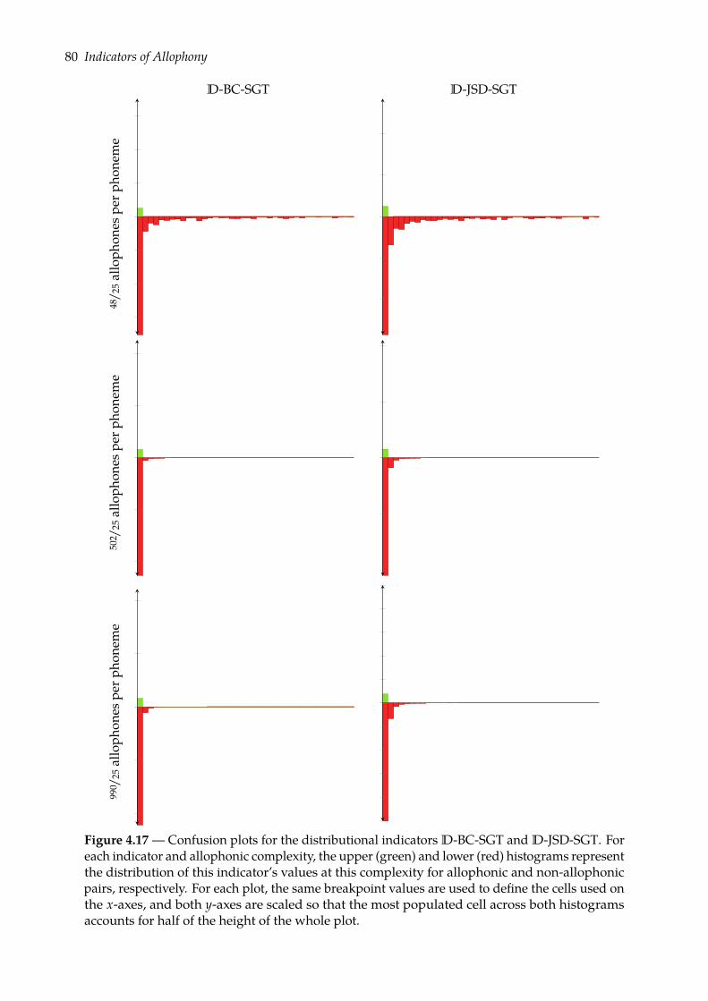
80 Indicators of Allophony
D-BC-SGT D-JSD-SGT
48/2
5alloph
ones
perp
hone
me
502 /
25alloph
ones
perp
hone
me
990 /
25alloph
ones
perp
hone
me
Figure 4.17 — Confusion plots for the distributional indicators D-BC-SGT and D-JSD-SGT. Foreach indicator and allophonic complexity, the upper (green) and lower (red) histograms representthe distribution of this indicator’s values at this complexity for allophonic and non-allophonicpairs, respectively. For each plot, the same breakpoint values are used to define the cells used onthe x-axes, and both y-axes are scaled so that the most populated cell across both histogramsaccounts for half of the height of the whole plot.
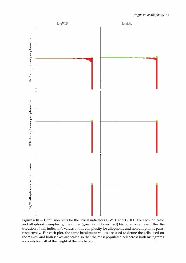
Prognoses of allophony 81
L-WTP L-HFL
48/2
5alloph
ones
perp
hone
me
502 /
25alloph
ones
perp
hone
me
990 /
25alloph
ones
perp
hone
me
Figure 4.18 — Confusion plots for the lexical indicators L-WTP and L-HFL. For each indicatorand allophonic complexity, the upper (green) and lower (red) histograms represent the dis-tribution of this indicator’s values at this complexity for allophonic and non-allophonic pairs,respectively. For each plot, the same breakpoint values are used to define the cells used onthe x-axes, and both y-axes are scaled so that the most populated cell across both histogramsaccounts for half of the height of the whole plot.
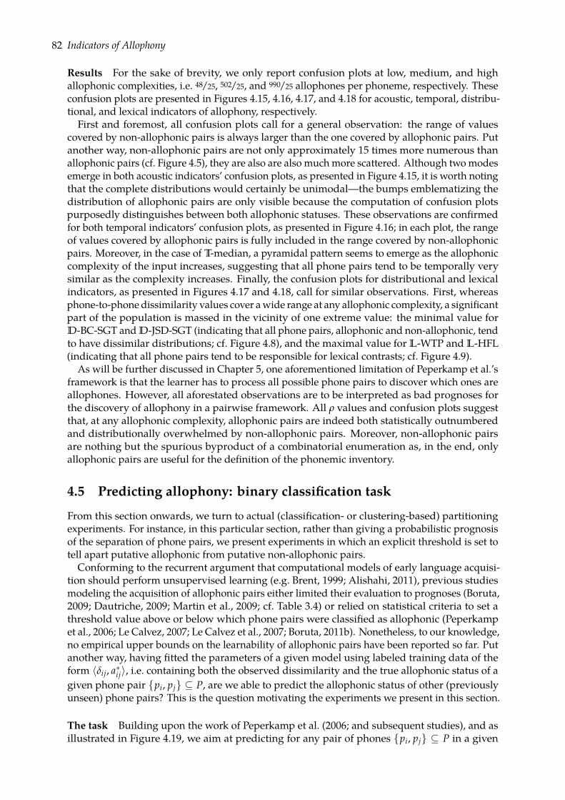
82 Indicators of Allophony
Results For the sake of brevity, we only report confusion plots at low, medium, and highallophonic complexities, i.e. 48/25, 502/25, and 990/25 allophones per phoneme, respectively. Theseconfusion plots are presented in Figures 4.15, 4.16, 4.17, and 4.18 for acoustic, temporal, distribu-tional, and lexical indicators of allophony, respectively.First and foremost, all confusion plots call for a general observation: the range of values
covered by non-allophonic pairs is always larger than the one covered by allophonic pairs. Putanother way, non-allophonic pairs are not only approximately 15 times more numerous thanallophonic pairs (cf. Figure 4.5), they are also are also muchmore scattered. Although twomodesemerge in both acoustic indicators’ confusion plots, as presented in Figure 4.15, it is worth notingthat the complete distributions would certainly be unimodal—the bumps emblematizing thedistribution of allophonic pairs are only visible because the computation of confusion plotspurposedly distinguishes between both allophonic statuses. These observations are confirmedfor both temporal indicators’ confusion plots, as presented in Figure 4.16; in each plot, the rangeof values covered by allophonic pairs is fully included in the range covered by non-allophonicpairs. Moreover, in the case of T-median, a pyramidal pattern seems to emerge as the allophoniccomplexity of the input increases, suggesting that all phone pairs tend to be temporally verysimilar as the complexity increases. Finally, the confusion plots for distributional and lexicalindicators, as presented in Figures 4.17 and 4.18, call for similar observations. First, whereasphone-to-phone dissimilarity values cover awide range at any allophonic complexity, a significantpart of the population is massed in the vicinity of one extreme value: the minimal value forD-BC-SGT and D-JSD-SGT (indicating that all phone pairs, allophonic and non-allophonic, tendto have dissimilar distributions; cf. Figure 4.8), and the maximal value for L-WTP and L-HFL(indicating that all phone pairs tend to be responsible for lexical contrasts; cf. Figure 4.9).
As will be further discussed in Chapter 5, one aforementioned limitation of Peperkamp et al.’sframework is that the learner has to process all possible phone pairs to discover which ones areallophones. However, all aforestated observations are to be interpreted as bad prognoses forthe discovery of allophony in a pairwise framework. All ρ values and confusion plots suggestthat, at any allophonic complexity, allophonic pairs are indeed both statistically outnumberedand distributionally overwhelmed by non-allophonic pairs. Moreover, non-allophonic pairsare nothing but the spurious byproduct of a combinatorial enumeration as, in the end, onlyallophonic pairs are useful for the definition of the phonemic inventory.
4.5 Predicting allophony: binary classification task
From this section onwards, we turn to actual (classification- or clustering-based) partitioningexperiments. For instance, in this particular section, rather than giving a probabilistic prognosisof the separation of phone pairs, we present experiments in which an explicit threshold is set totell apart putative allophonic from putative non-allophonic pairs.Conforming to the recurrent argument that computational models of early language acquisi-
tion should perform unsupervised learning (e.g. Brent, 1999; Alishahi, 2011), previous studiesmodeling the acquisition of allophonic pairs either limited their evaluation to prognoses (Boruta,2009; Dautriche, 2009; Martin et al., 2009; cf. Table 3.4) or relied on statistical criteria to set athreshold value above or below which phone pairs were classified as allophonic (Peperkampet al., 2006; Le Calvez, 2007; Le Calvez et al., 2007; Boruta, 2011b). Nonetheless, to our knowledge,no empirical upper bounds on the learnability of allophonic pairs have been reported so far. Putanother way, having fitted the parameters of a given model using labeled training data of theform 〈δij, a∗ij〉, i.e. containing both the observed dissimilarity and the true allophonic status of agiven phone pair pi, pj ⊆ P, are we able to predict the allophonic status of other (previouslyunseen) phone pairs? This is the question motivating the experiments we present in this section.
The task Building upon the work of Peperkamp et al. (2006; and subsequent studies), and asillustrated in Figure 4.19, we aim at predicting for any pair of phones pi, pj ⊆ P in a given
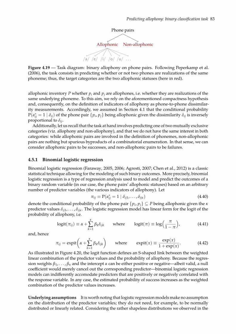
Predicting allophony: binary classification task 83
Phone pairs
Allophonic
/a/ /e/ /i/ /o/ /u/ . . .
Non-allophonic
Figure 4.19 — Task diagram: binary allophony on phone pairs. Following Peperkamp et al.(2006), the task consists in predicting whether or not two phones are realizations of the samephoneme; thus, the target categories are the two allophonic statuses (here in red).
allophonic inventory P whether pi and pj are allophones, i.e. whether they are realizations of thesame underlying phoneme. To this aim, we rely on the aforementioned compactness hypothesisand, consequently, on the definition of indicators of allophony as phone-to-phone dissimilar-ity measurements. Accordingly, we assumed in Section 4.1 that the conditional probabilityP(a∗ij = 1 | δij) of the phone pair pi, pj being allophonic given the dissimilarity δij is inverselyproportional to δij.
Additionally, let us recall that the task at hand involves predicting one of twomutually exclusivecategories (viz. allophony and non-allophony), and that we do not have the same interest in bothcategories: while allophonic pairs are involved in the definition of phonemes, non-allophonicpairs are nothing but spurious byproducts of a combinatorial enumeration. In that sense, we canconsider allophonic pairs to be successes, and non-allophonic pairs to be failures.
4.5.1 Binomial logistic regression
Binomial logistic regression (Faraway, 2005, 2006; Agresti, 2007; Chen et al., 2012) is a classicstatistical technique allowing for themodeling of such binary outcomes. More precisely, binomiallogistic regression is a type of regression analysis used to model and predict the outcomes of abinary random variable (in our case, the phone pairs’ allophonic statuses) based on an arbitrarynumber of predictor variables (the various indicators of allophony). Let
πij ≡ P(a∗ij = 1 | δij1, . . . , δijκ) (4.40)denote the conditional probability of the phone pair pi, pj ⊆ P being allophonic given the κpredictor values δij1, . . . , δijκ. The logistic regression model has linear form for the logit of theprobability of allophony, i.e.
logit(πij) ≡ α +κ
∑k=1
βkδijk where logit(π) ≡ log( π
1− π
), (4.41)
and, hence
πij = expit(
α +κ
∑k=1
βkδijk
)where expit(x) ≡ exp(x)
1 + exp(x). (4.42)
As illustrated in Figure 4.20, the logit function defines an S-shaped link between the weightedlinear combination of the predictor values and the probability of allophony. Because the regres-sion weights β1, . . . , βκ and the intercept α can be either positive or negative—albeit valid, a nullcoefficient would merely cancel out the corresponding predictor—binomial logistic regressionmodels can indifferently accomodate predictors that are positively or negatively correlated withthe response variable. In any case, the estimated probability of success increases as the weightedcombination of the predictor values increases.
Underlying assumptions It isworth noting that logistic regressionmodelsmake no assumptionon the distribution of the predictor variables; they do not need, for example, to be normallydistributed or linearly related. Considering the rather shapeless distributions we observed in the
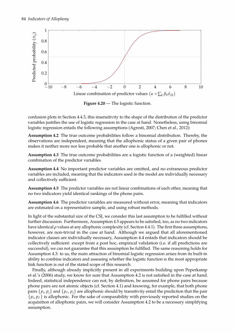
84 Indicators of Allophony
−10 −8 −6 −4 −2 0 2 4 6 8 100
0.2
0.4
0.6
0.8
1
Linear combination of predictor values(α +∑k βkδijk
)
Pred
icte
dpr
obab
ility
(πij)
Figure 4.20 — The logistic function.
confusion plots in Section 4.4.3, this insensitivity to the shape of the distribution of the predictorvariables justifies the use of logistic regression in the case at hand. Nonetheless, using binomiallogistic regression entails the following assumptions (Agresti, 2007; Chen et al., 2012):
Assumption 4.2 The true outcome probabilities follow a binomial distribution. Thereby, theobservations are independent, meaning that the allophonic status of a given pair of phonesmakes it neither more nor less probable that another one is allophonic or not.
Assumption 4.3 The true outcome probabilities are a logistic function of a (weighted) linearcombination of the predictor variables.
Assumption 4.4 No important predictor variables are omitted, and no extraneous predictorvariables are included, meaning that the indicators used in the model are individually necessaryand collectively sufficient.
Assumption 4.5 The predictor variables are not linear combinations of each other, meaning thatno two indicators yield identical rankings of the phone pairs.
Assumption 4.6 The predictor variables are measured without error, meaning that indicatorsare estimated on a representative sample, and using robust methods.
In light of the substantial size of the CSJ, we consider this last assumption to be fulfilled withoutfurther discussion. Furthermore, Assumption 4.5 appears to be satisfied, too, as no two indicatorshave identical ρ values at any allophonic complexity (cf. Section 4.4.1). The first three assumptions,however, are non-trivial in the case at hand. Although we argued that all aforementionedindicator classes are individually necessary, Assumption 4.4 entails that indicators should becollectively sufficient: except from a post hoc, empirical validation (i.e. if all predictions aresuccessful), we can not guarantee that this assumption be fulfilled. The same reasoning holds forAssumption 4.3: to us, the main attraction of binomial logistic regression arises from its built-inability to combine indicators and assessing whether the logistic function is the most appropriatelink function is out of the stated scope of this research.Finally, although already implicitly present in all experiments building upon Peperkamp
et al.’s (2006) study, we know for sure that Assumption 4.2 is not satisfied in the case at hand.Indeed, statistical independence can not, by definition, be assumed for phone pairs becausephone pairs are not atomic objects (cf. Section 4.1) and knowing, for example, that both phonepairs pi, pj and pi′ , pj are allophonic should by transitivity entail the prediction that the pairpi, pi′ is allophonic. For the sake of comparability with previously reported studies on theacquisition of allophonic pairs, we will consider Assumption 4.2 to be a necessary simplifyingassumption.
Predicting allophony: binary classification task 85
Model-fitting In the case of binomial logistic regression, fitting the model consists in esti-mating the regression parameters β1, . . . , βκ and the intercept α from a given a set of trainingobservations of the form 〈δij1, . . . , δijκ, wij, a∗ij〉, i.e. comprising the dissimilarity ratings assignedto a given phone pair pi, pj, its weight, and its true allophonic status. Exposing the detailsof the estimation process is beyond the scope of the present study. Suffice it to say that thenumerical algorithm we used outputs the parameter values that maximize the log-likelihoodof the parameters given the training data (Agresti, 2007; R Development Core Team, 2010; cf.stats::glm). Adapting the definition given by Faraway (2006; pp. 30, 129) to our notation, thelog-likelihood function is given by
log-likelihood(α, β1, . . . , βκ; A∗, W) ≡∑i<j
a∗ij logit(πij)− wij logit(πij) + log(
wij
a∗ijwij
). (4.43)
As pointed out by Agresti (2007), a desirable property of regression models is that they smooththe sample data, somewhat dampening the observed variability.
It is worth mentioning that if any predictor variable indicates a complete separation of the twoclasses (i.e. if there is a value at and abovewhich all observations are successes and belowwhich allobservations are failures, or vice versa), the estimation of the parameters by maximum likelihoodis made impossible (Chen et al., 2012). In the case at hand, however, we already observed that nopredictor contains such ideal data. Indeed, the probabilistic prognosis of allophony we presentedin Section 4.4.1 is nothing but a numerical assessement of class separation, and for no indicatordid we observe ρ values equal to 1, at any allophonic complexity.
Individual and quartet models Because, to our knowledge, these experiments are the firstattempt at using binomial logistic regression to model the acquisition of allophony, and becausemany indicators of allophony were introduced in the present study, we compare the performanceof regression models relying on a single indicator (i.e. κ = 1, referred to as individual models)to that of models relying on a combination comprising one indicator of each class (i.e. κ = 4,referred to as quartet models). As we reduced the number of indicators of allophony to twoindicators per class, viz.
A-DTWA-MBD
×
T-medianT-range
×
D-JSD-SGTD-BC-SGT
×
L-WTPL-HFL
,
there are 2× 4 = 8 possible individual models and, consequently, 24 = 16 possible quartetmodels. Unless otherwise specified, logistic regression models rely on the aforementioned rangestandardization of the indicators. However, as discussed in Section 4.3.2, these experimentsaddress an additional, transversal issue, viz. deciding whether allophony can be learned from amere ranking of an indicator’s values or if the relative values bring additional information. Forthis reason, each of the 8 + 16 = 24 regression models will be evaluated on both the range- andthe rank-based standardization of the indicators’ data.
4.5.2 Evaluation
In these experiments, we are not interested in the interpretation of the estimated regressionparameters, but in the predictive power of the regression models. For the purpose of classifyingcandidate phone pairs as allophonic or non-allophonic, we rely on the standard threshold ofπij > .5 whereby a given phone pair pi, pj is considered to be allophonic, i.e. when
P(a∗ij = 1 | δij1, . . . , δijκ) > P(a∗ij = 0 | δij1, . . . , δijκ). (4.44)As a matter of convenience, let A ≡ [aij] denote the predicted matrix of allophony whereaij ≡ Jπij > .5K denotes the predicted allophonic status of the pair pi, pj.
Confirmatory overfitting Generally speaking, predictive models are trained and tested ondistinct sets of observations so as to avoid overfitting, and binomial logistic regression models
86 Indicators of Allophony
are no exception. Overfitting can be defined as the discovery of apparent predictive relations inthe training data (i.e. between the predictor variables δij1, . . . , δijκ and the true outcome a∗ij) thatdo not hold in general. Using distinct yet comparable observation sets allows for an assessmentof the overfitting of the model parameters to the training data: if a given model fits both thetraining and the test data, it is unlikely that overfitting occurred; by contrast, if a model fits thetraining data much better than the test data, then one can suspect the model to be overfitted.
However, in the case at hand, we aim at providing empirical upper bounds on the learnabilityof allophony and, therefore, chose to perform supervised learning to place ourselves in a best-casescenario. To further help the discovery of the dichotomy between allophonic and non-allophonicpairs, we purposedly use all available data for both the training and the evaluation of ourregression models, a setup we tentatively refer to as confirmatory overfitting. Put another way,given all available data, and including the reference matrix of allophony A∗, can we tell apartallophonic and non-allophonic pairs?It is worth noting that we did perform more reasonable tests in preliminary experiments.
Indeed, for all individual and quartet models, we compared their predictive power using con-firmatory overfitting and two standard techniques of cross-validation. First, we carried outevaluations using a technique known as tenfold cross-validation, whereby all available observa-tions are partitioned into 10 subsamples, 1 subsample is reserved as the test set and the remaining9 are used as the training set; this process being repeated 10 times so that each subsample isused exactly once as the test set. Second, we carried out evaluations using a cross-validationtechnique known as leave-one-out validation, whereby a single observation is reserved as thetest set and all other observations are used as the training data; this process being repeated sothat each each observation is used exactly once as the test set. Because these techniques requirethat a considerable number of regression models be trained—10 and n(n − 1)/2 for tenfoldand leave-one-out cross-validation, respectively, for each of the 24 models and the 20 testedallophonic complexities—they are computationally prohibitive. Accordingly, these preliminaryexperiments were only carried out for the lowest allophonic complexities, viz. 48/25, 98/25, and147/25 allophones per phoneme. For all benchmarked models and complexities, the difference inperformance between confirmatory overfitting and both cross-validations techniques did notexceed ±2% of accuracy, thus indicating that confirmatory overfitting does not have a significantimpact on the predictive power of the models.
Goodness of fit The first quantitative criterion we use to assess the fit of a binomial logisticregression model to the reference outcomes collected in A∗ is known as the Akaike informationcriterion (henceforth AIC; Akaike, 1974). The major piece of information the AIC relies on is thepreviously defined likelihood function (cf. Equation 4.43). Indeed, the AIC of a given binomiallogistic regression model is given by the maximized value of the likelihood function for itsparameters, penalized by the number of such parameters. Concretely, it is defined as
AIC(α, β1, . . . , βκ; A∗, W) ≡ −2(log-likelihood(α, β1, . . . , βκ; A∗, W)− (κ + 1)
)(4.45)
where β1, . . . , βκ and α denote the estimated optimal paramater values. It is worth noting thatthe last term κ + 1 matches the number of such parameters in the model (κ distinct βk coefficients,plus one α coefficient). The penalty accounts for the fact that increasing the number of parameters(i.e. of predictor variables) tends to increase the goodness of fit, regardless of the true number ofparameters that may sufficiently account for the observations. Regression models with a goodfit tend to minimize the AIC (i.e. the lower the better; Faraway, 2005).Because the AIC does not rely on a partition of, for a given allophonic inventory, all possible
phone pairs into allophonic and non-allophonic pairs, and following the discussion in Section 4.4,this criterion is to be considered as a prognosis rather than as a true evaluation measure.
Contingency table The other quantitative criteria we use to assess the performance of binomiallogistic regression models rely on the models’ predictive power. For each model, a contingencytable (a.k.a. confusion matrix or classification table) is used to cross-classify the true outcomes
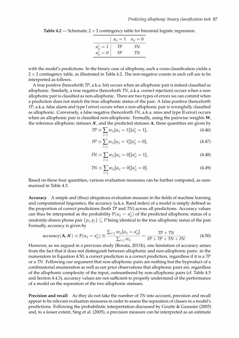
Predicting allophony: binary classification task 87
Table 4.2 — Schematic 2× 2 contingency table for binomial logistic regression.
aij = 1 aij = 0
a∗ij = 1 TP FNa∗ij = 0 FP TN
with the model’s predictions. In the binary case of allophony, such a cross-classification yields a2× 2 contingency table, as illustrated in Table 4.2. The non-negative counts in each cell are to beinterpreted as follows.
A true positive (henceforth TP, a.k.a. hit) occurs when an allophonic pair is indeed classified asallophonic. Similarly, a true negative (henceforth TN, a.k.a. correct rejection) occurs when a non-allophonic pair is classified as non-allophonic. There are two types of errors we can commit whena prediction does not match the true allophonic status of the pair. A false positive (henceforthFP, a.k.a. false alarm and type I error) occurs when a non-allophonic pair is wrongfully classifiedas allophonic. Conversely, a false negative (henceforth FN, a.k.a. miss and type II error) occurswhen an allophonic pair is classified non-allophonic. Formally, using the pairwise weights W,the reference allophonic statuses A∗, and the predicted statuses A, these quantities are given by
TP ≡∑i<j
wijJaij = 1KJa∗ij = 1K, (4.46)
FP ≡∑i<j
wijJaij = 1KJa∗ij = 0K, (4.47)
FN ≡∑i<j
wijJaij = 0KJa∗ij = 1K, (4.48)
TN ≡∑i<j
wijJaij = 0KJa∗ij = 0K. (4.49)
Based on these four quantities, various evaluation measures can be further computed, as sum-marized in Table 4.3.
Accuracy A simple and (thus) ubiquitous evaluation measure in the fields of machine learningand computational linguistics, the accuracy (a.k.a. Rand index) of a model is simply defined asthe proportion of correct predictions (both TP and TN) across all predictions. Accuracy valuescan thus be interpreted as the probability P(aij = a∗ij) of the predicted allophonic status of arandomly-drawn phone pair pi, pj ⊆ P being identical to the true allophonic status of the pair.Formally, accuracy is given by
accuracy(A, A∗) ≡ P(aij = a∗ij) u∑i<j wijJaij = a∗ijK
∑i<j wij=
TP + TNFP + TP + TN + FN
. (4.50)
However, as we argued in a previous study (Boruta, 2011b), one limitation of accuracy arisesfrom the fact that it does not distinguish between allophonic and non-allophonic pairs: in thenumerators in Equation 4.50, a correct prediction is a correct prediction, regardless if it is a TPor a TN. Following our argument that non-allophonic pairs are nothing but the byproduct of acombinatorial enumeration as well as our prior observations that allophonic pairs are, regardlessof the allophonic complexity of the input, outnumbered by non-allophonic pairs (cf. Table 4.5and Section 4.4.3), accuracy values are not sufficient to properly understand of the performanceof a model on the separation of the two allophonic statuses.
Precision and recall As they do not take the number of TN into account, precision and recallappear to be relevant evaluation measures in order to assess the separation of classes in a model’spredictions. Following the probabilistic interpretation discussed by Goutte & Gaussier (2005)and, to a lesser extent, Sing et al. (2005), a precision measure can be interpreted as an estimate
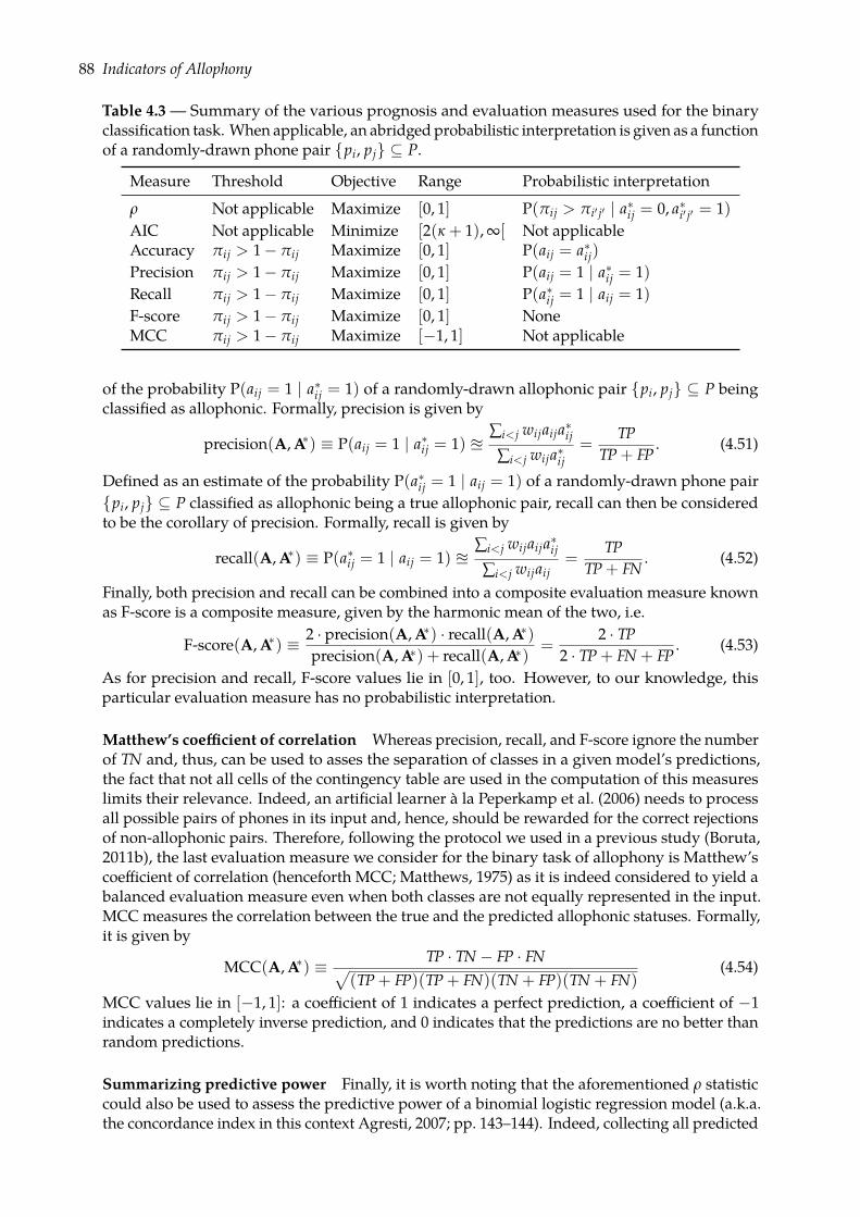
88 Indicators of Allophony
Table 4.3 — Summary of the various prognosis and evaluation measures used for the binaryclassification task. When applicable, an abridged probabilistic interpretation is given as a functionof a randomly-drawn phone pair pi, pj ⊆ P.
Measure Threshold Objective Range Probabilistic interpretation
ρ Not applicable Maximize [0, 1] P(πij > πi′ j′ | a∗ij = 0, a∗i′ j′ = 1)AIC Not applicable Minimize [2(κ + 1), ∞[ Not applicableAccuracy πij > 1− πij Maximize [0, 1] P(aij = a∗ij)Precision πij > 1− πij Maximize [0, 1] P(aij = 1 | a∗ij = 1)Recall πij > 1− πij Maximize [0, 1] P(a∗ij = 1 | aij = 1)F-score πij > 1− πij Maximize [0, 1] NoneMCC πij > 1− πij Maximize [−1, 1] Not applicable
of the probability P(aij = 1 | a∗ij = 1) of a randomly-drawn allophonic pair pi, pj ⊆ P beingclassified as allophonic. Formally, precision is given by
precision(A, A∗) ≡ P(aij = 1 | a∗ij = 1) u∑i<j wijaija∗ij∑i<j wija∗ij
=TP
TP + FP. (4.51)
Defined as an estimate of the probability P(a∗ij = 1 | aij = 1) of a randomly-drawn phone pairpi, pj ⊆ P classified as allophonic being a true allophonic pair, recall can then be consideredto be the corollary of precision. Formally, recall is given by
recall(A, A∗) ≡ P(a∗ij = 1 | aij = 1) u∑i<j wijaija∗ij∑i<j wijaij
=TP
TP + FN. (4.52)
Finally, both precision and recall can be combined into a composite evaluation measure knownas F-score is a composite measure, given by the harmonic mean of the two, i.e.
F-score(A, A∗) ≡ 2 · precision(A, A∗) · recall(A, A∗)precision(A, A∗) + recall(A, A∗)
=2 · TP
2 · TP + FN + FP. (4.53)
As for precision and recall, F-score values lie in [0, 1], too. However, to our knowledge, thisparticular evaluation measure has no probabilistic interpretation.
Matthew’s coefficient of correlation Whereas precision, recall, and F-score ignore the numberof TN and, thus, can be used to asses the separation of classes in a given model’s predictions,the fact that not all cells of the contingency table are used in the computation of this measureslimits their relevance. Indeed, an artificial learner à la Peperkamp et al. (2006) needs to processall possible pairs of phones in its input and, hence, should be rewarded for the correct rejectionsof non-allophonic pairs. Therefore, following the protocol we used in a previous study (Boruta,2011b), the last evaluation measure we consider for the binary task of allophony is Matthew’scoefficient of correlation (henceforth MCC; Matthews, 1975) as it is indeed considered to yield abalanced evaluation measure even when both classes are not equally represented in the input.MCC measures the correlation between the true and the predicted allophonic statuses. Formally,it is given by
MCC(A, A∗) ≡ TP · TN − FP · FN√(TP + FP)(TP + FN)(TN + FP)(TN + FN)
(4.54)
MCC values lie in [−1, 1]: a coefficient of 1 indicates a perfect prediction, a coefficient of −1indicates a completely inverse prediction, and 0 indicates that the predictions are no better thanrandom predictions.
Summarizing predictive power Finally, it is worth noting that the aforementioned ρ statisticcould also be used to assess the predictive power of a binomial logistic regression model (a.k.a.the concordance index in this context Agresti, 2007; pp. 143–144). Indeed, collecting all predicted
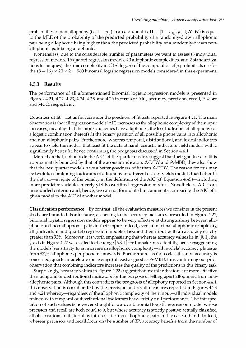
Predicting allophony: binary classification task 89
probabilities of non-allophony (i.e. 1− πij) in an n× n matrix Π ≡ [1− πij], ρ(Π; A∗, W) is equalto the MLE of the probability of the predicted probability of a randomly-drawn allophonicpair being allophonic being higher than the predicted probability of a randomly-drawn non-allophonic pair being allophonic.Nonetheless, due to the considerable number of parameters we want to assess (8 individual
regression models, 16 quartet regression models, 20 allophonic complexities, and 2 standardiza-tions techniques), the time complexity inO(n2 log2 n) of the computation of ρ prohibits its use forthe (8 + 16)× 20× 2 = 960 binomial logistic regression models considered in this experiment.
4.5.3 Results
The performance of all aforementioned binomial logistic regression models is presented inFigures 4.21, 4.22, 4.23, 4.24, 4.25, and 4.26 in terms of AIC, accuracy, precision, recall, F-scoreand MCC, respectively.
Goodness of fit Let us first consider the goodness of fit tests reported in Figure 4.21. The mainobservation is that all regressionmodels’ AIC increases as the allophonic complexity of their inputincreases, meaning that the more phonemes have allophones, the less indicators of allophony (ora logistic combination thereof) fit the binary partition of all possible phone pairs into allophonicand non-allophonic pairs. Furthermore, whereas temporal, distributional, and lexical indicatorsappear to yield the models that least fit the data at hand, acoustic indicators yield models with asignificantly better fit, hence confirming the prognosis discussed in Section 4.4.1.
More than that, not only do the AICs of the quartet models suggest that their goodness of fit isapproximately bounded by that of the acoustic indicators A-DTW and A-MBD, they also showthat the best quartet models have a better goodness of fit than A-DTW. The reason for this maybe twofold: combining indicators of allophony of different classes yields models that better fitthe data or—in spite of the penalty in the definition of the AIC (cf. Equation 4.45)—includingmore predictor variables merely yields overfitted regression models. Nonetheless, AIC is anunbounded criterion and, hence, we can not formulate but comments comparing the AIC of agiven model to the AIC of another model.
Classification performance By contrast, all the evaluation measures we consider in the presentstudy are bounded. For instance, according to the accuracy measures presented in Figure 4.22,binomial logistic regression models appear to be very effective at distinguishing between allo-phonic and non-allophonic pairs in their input: indeed, even at maximal allophonic complexity,all (individual and quartet) regression models classified their input with an accuracy strictlygreater than 93%. Moreover, it is worth emphasizing that whereas accuracy values lie in [0, 1], they-axis in Figure 4.22 was scaled to the range [.93, 1] for the sake of readability, hence exaggeratingthe models’ sensitivity to an increase in allophonic complexity—all models’ accuracy plateausfrom 450/25 allophones per phoneme onwards. Furthermore, as far as classification accuracy isconcerned, quartet models are (on average) at least as good as A-MBD, thus confirming our priorobservation that combining indicators increases the quality of the predictions in this binary task.Surprisingly, accuracy values in Figure 4.22 suggest that lexical indicators are more effective
than temporal or distributional indicators for the purpose of telling apart allophonic from non-allophonic pairs. Although this contradicts the prognosis of allophony reported in Section 4.4.1,this observation is corroborated by the precision and recall measures reported in Figures 4.23and 4.24 whereby—regardless of the allophonic complexity of their input—all individual modelstrained with temporal or distributional indicators have strictly null performance. The interpre-tation of such values is however straightforward: a binomial logistic regression model whoseprecision and recall are both equal to 0, but whose accuracy is strictly positive actually classifiedall observations in its input as failures—i.e. non-allophonic pairs in the case at hand. Indeed,whereas precision and recall focus on the number of TP, accuracy benefits from the number of
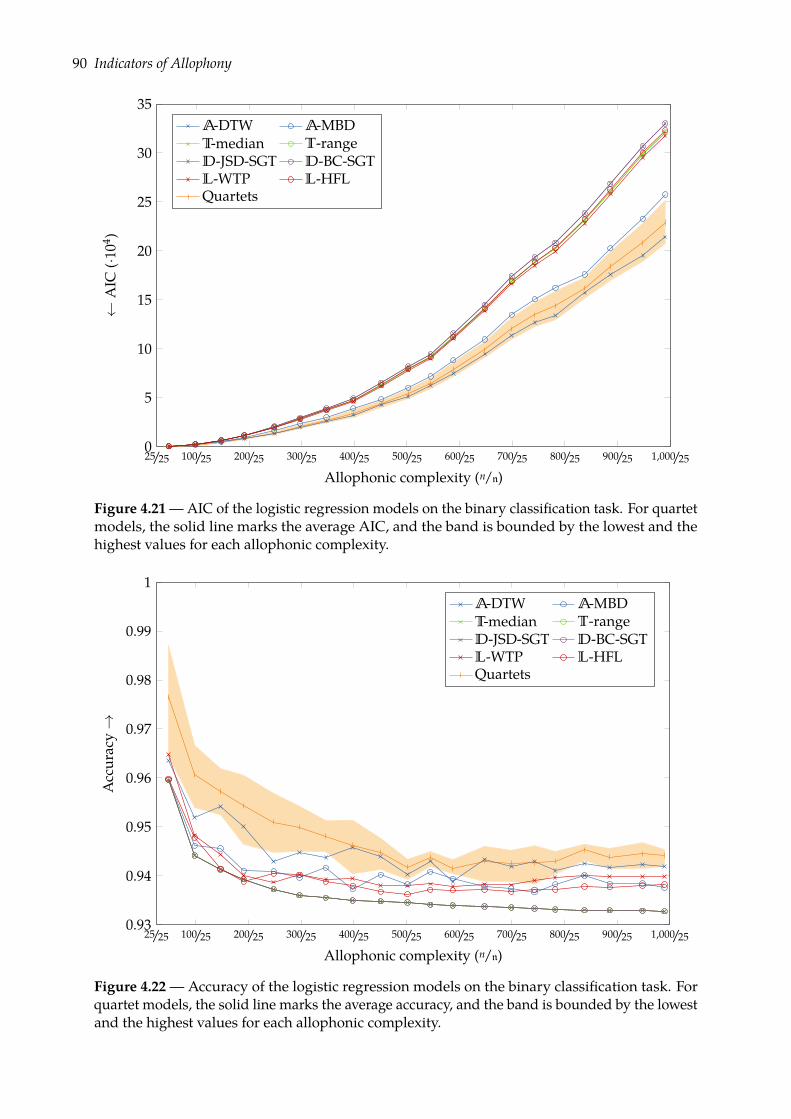
90 Indicators of Allophony
100/25 200/25 300/25 400/25 500/25 600/25 700/25 800/25 900/25 1,000/250
5
10
15
20
25
30
35
25/25
Allophonic complexity (n/n)
←A
IC(·1
04 )A-DTW A-MBDT-median T-rangeD-JSD-SGT D-BC-SGTL-WTP L-HFLQuartets
Figure 4.21—AIC of the logistic regression models on the binary classification task. For quartetmodels, the solid line marks the average AIC, and the band is bounded by the lowest and thehighest values for each allophonic complexity.
100/25 200/25 300/25 400/25 500/25 600/25 700/25 800/25 900/25 1,000/250.93
0.94
0.95
0.96
0.97
0.98
0.99
1
25/25
Allophonic complexity (n/n)
Acc
urac
y→
A-DTW A-MBDT-median T-rangeD-JSD-SGT D-BC-SGTL-WTP L-HFLQuartets
Figure 4.22—Accuracy of the logistic regression models on the binary classification task. Forquartet models, the solid line marks the average accuracy, and the band is bounded by the lowestand the highest values for each allophonic complexity.
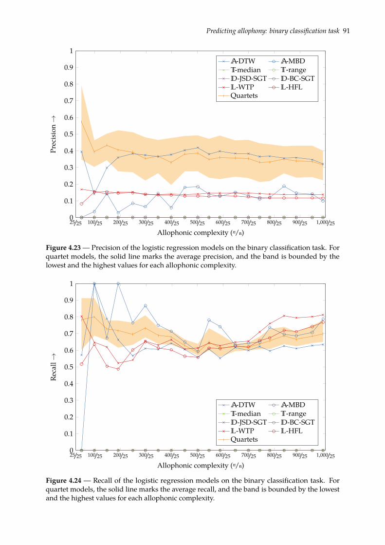
Predicting allophony: binary classification task 91
100/25 200/25 300/25 400/25 500/25 600/25 700/25 800/25 900/25 1,000/250
0.1
0.2
0.3
0.4
0.5
0.6
0.7
0.8
0.9
1
25/25
Allophonic complexity (n/n)
Prec
isio
n→
A-DTW A-MBDT-median T-rangeD-JSD-SGT D-BC-SGTL-WTP L-HFLQuartets
Figure 4.23— Precision of the logistic regression models on the binary classification task. Forquartet models, the solid line marks the average precision, and the band is bounded by thelowest and the highest values for each allophonic complexity.
100/25 200/25 300/25 400/25 500/25 600/25 700/25 800/25 900/25 1,000/250
0.1
0.2
0.3
0.4
0.5
0.6
0.7
0.8
0.9
1
25/25
Allophonic complexity (n/n)
Reca
ll→
A-DTW A-MBDT-median T-rangeD-JSD-SGT D-BC-SGTL-WTP L-HFLQuartets
Figure 4.24 — Recall of the logistic regression models on the binary classification task. Forquartet models, the solid line marks the average recall, and the band is bounded by the lowestand the highest values for each allophonic complexity.
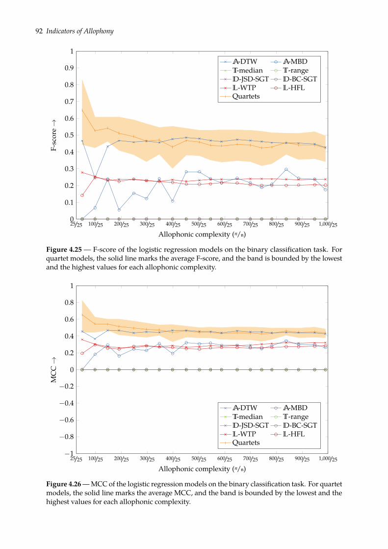
92 Indicators of Allophony
100/25 200/25 300/25 400/25 500/25 600/25 700/25 800/25 900/25 1,000/250
0.1
0.2
0.3
0.4
0.5
0.6
0.7
0.8
0.9
1
25/25
Allophonic complexity (n/n)
F-sc
ore→
A-DTW A-MBDT-median T-rangeD-JSD-SGT D-BC-SGTL-WTP L-HFLQuartets
Figure 4.25 — F-score of the logistic regression models on the binary classification task. Forquartet models, the solid line marks the average F-score, and the band is bounded by the lowestand the highest values for each allophonic complexity.
100/25 200/25 300/25 400/25 500/25 600/25 700/25 800/25 900/25 1,000/25−1
−0.8
−0.6
−0.4
−0.2
0
0.2
0.4
0.6
0.8
1
25/25
Allophonic complexity (n/n)
MC
C→
A-DTW A-MBDT-median T-rangeD-JSD-SGT D-BC-SGTL-WTP L-HFLQuartets
Figure 4.26—MCC of the logistic regressionmodels on the binary classification task. For quartetmodels, the solid line marks the average MCC, and the band is bounded by the lowest and thehighest values for each allophonic complexity.
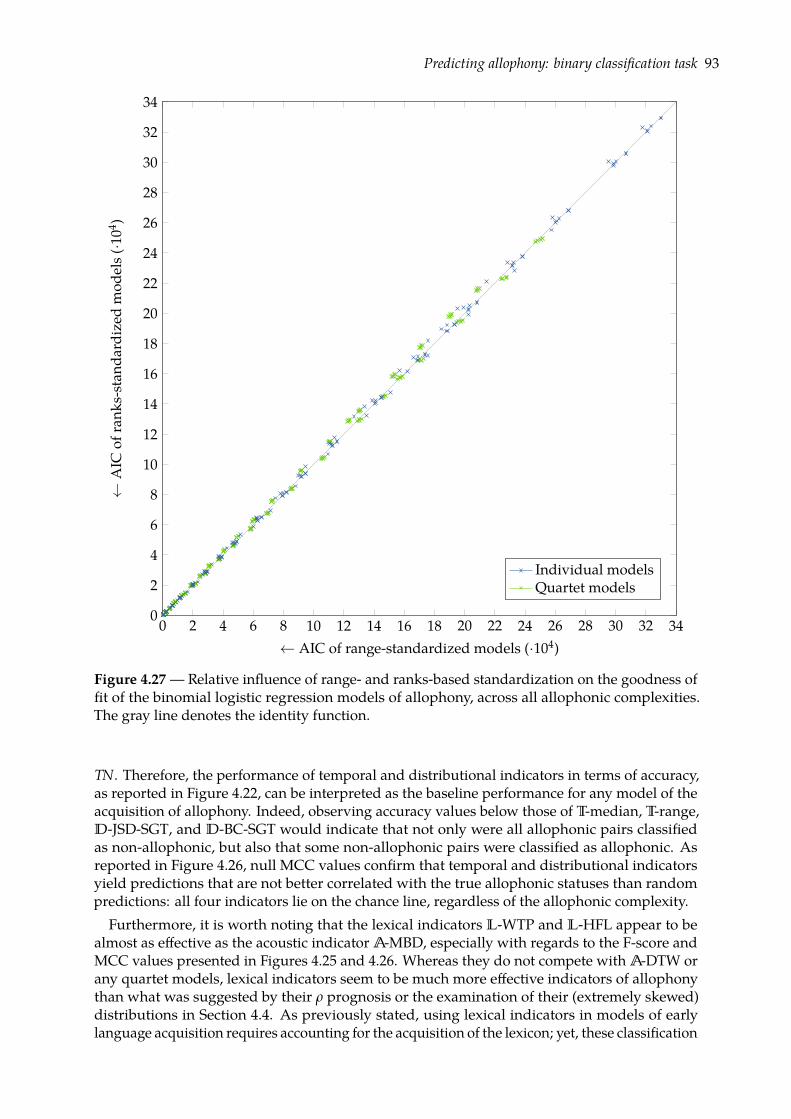
Predicting allophony: binary classification task 93
0 2 4 6 8 10 12 14 16 18 20 22 24 26 28 30 32 340
2
4
6
8
10
12
14
16
18
20
22
24
26
28
30
32
34
← AIC of range-standardized models (·104)
←A
ICof
rank
s-st
anda
rdiz
edm
odel
s(·10
4 )
Individual modelsQuartet models
Figure 4.27 — Relative influence of range- and ranks-based standardization on the goodness offit of the binomial logistic regression models of allophony, across all allophonic complexities.The gray line denotes the identity function.
TN. Therefore, the performance of temporal and distributional indicators in terms of accuracy,as reported in Figure 4.22, can be interpreted as the baseline performance for any model of theacquisition of allophony. Indeed, observing accuracy values below those of T-median, T-range,D-JSD-SGT, and D-BC-SGT would indicate that not only were all allophonic pairs classifiedas non-allophonic, but also that some non-allophonic pairs were classified as allophonic. Asreported in Figure 4.26, null MCC values confirm that temporal and distributional indicatorsyield predictions that are not better correlated with the true allophonic statuses than randompredictions: all four indicators lie on the chance line, regardless of the allophonic complexity.
Furthermore, it is worth noting that the lexical indicators L-WTP and L-HFL appear to bealmost as effective as the acoustic indicator A-MBD, especially with regards to the F-score andMCC values presented in Figures 4.25 and 4.26. Whereas they do not compete with A-DTW orany quartet models, lexical indicators seem to be much more effective indicators of allophonythan what was suggested by their ρ prognosis or the examination of their (extremely skewed)distributions in Section 4.4. As previously stated, using lexical indicators in models of earlylanguage acquisition requires accounting for the acquisition of the lexicon; yet, these classification
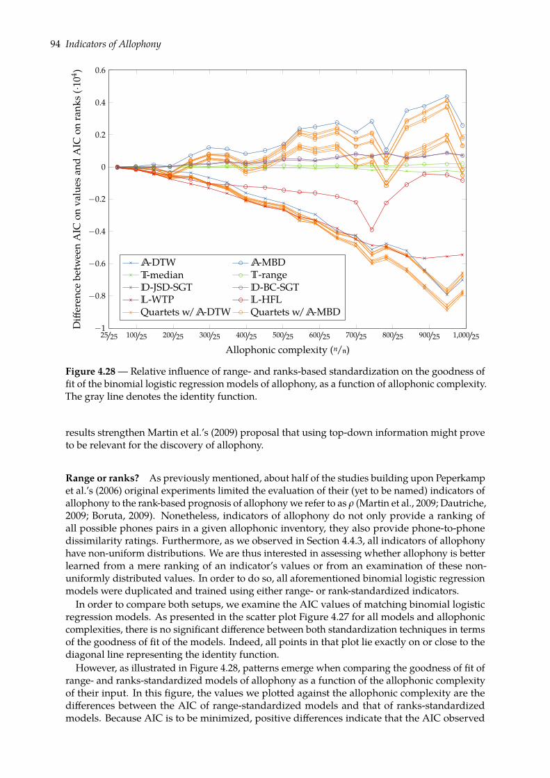
94 Indicators of Allophony
100/25 200/25 300/25 400/25 500/25 600/25 700/25 800/25 900/25 1,000/25−1
−0.8
−0.6
−0.4
−0.2
0
0.2
0.4
0.6
25/25
Allophonic complexity (n/n)
Differen
cebe
tweenAIC
onva
lues
andAIC
onrank
s(·10
4 )
A-DTW A-MBDT-median T-rangeD-JSD-SGT D-BC-SGTL-WTP L-HFLQuartets w/A-DTW Quartets w/A-MBD
Figure 4.28 — Relative influence of range- and ranks-based standardization on the goodness offit of the binomial logistic regression models of allophony, as a function of allophonic complexity.The gray line denotes the identity function.
results strengthen Martin et al.’s (2009) proposal that using top-down information might proveto be relevant for the discovery of allophony.
Range or ranks? As previously mentioned, about half of the studies building upon Peperkampet al.’s (2006) original experiments limited the evaluation of their (yet to be named) indicators ofallophony to the rank-based prognosis of allophonywe refer to as ρ (Martin et al., 2009; Dautriche,2009; Boruta, 2009). Nonetheless, indicators of allophony do not only provide a ranking ofall possible phones pairs in a given allophonic inventory, they also provide phone-to-phonedissimilarity ratings. Furthermore, as we observed in Section 4.4.3, all indicators of allophonyhave non-uniform distributions. We are thus interested in assessing whether allophony is betterlearned from a mere ranking of an indicator’s values or from an examination of these non-uniformly distributed values. In order to do so, all aforementioned binomial logistic regressionmodels were duplicated and trained using either range- or rank-standardized indicators.In order to compare both setups, we examine the AIC values of matching binomial logistic
regression models. As presented in the scatter plot Figure 4.27 for all models and allophoniccomplexities, there is no significant difference between both standardization techniques in termsof the goodness of fit of the models. Indeed, all points in that plot lie exactly on or close to thediagonal line representing the identity function.
However, as illustrated in Figure 4.28, patterns emerge when comparing the goodness of fit ofrange- and ranks-standardized models of allophony as a function of the allophonic complexityof their input. In this figure, the values we plotted against the allophonic complexity are thedifferences between the AIC of range-standardized models and that of ranks-standardizedmodels. Because AIC is to be minimized, positive differences indicate that the AIC observed
Overall assessment 95
on values is lesser than the AIC observed on ranks and, hence, that using the true values of thecorresponding indicator(s) yield a better-fitting model. Surprisingly, temporal indicators areinsensitive to both allophonic complexity and the standardization of their input. This observationis however supported by the confusion plots in Section 4.4.3 and, especially, Figure 4.16 wherebyT-median and T-range appear to have the most uniform distributions (yet shapeless). The moststriking pattern in Figure 4.28 is, however, that the goodness of fit values for quartet modelsfollow two strong, distinct trends depending on the acoustic indicator they comprise. On onehand, A-DTW and quartets that include A-DTW seem to benefit from a mere ranking of thevalues. On the other hand, A-MBD and quartets that include A-MBD seem to benefit from thetrue values of the indicators. Yet, both acoustic indicators have comparable confusion plots,as illustrated in Figure 4.15. Further research is thus needed to take a stance on the issue ofstandardization, as will be discussed in Chapter 5.
4.6 Overall assessment
In this chapter, we defined a common framework for all phone-to-phone (dis)similarity measuresproposed in studies building upon Peperkamp et al.’s original experiments (Peperkamp et al.,2006; Le Calvez, 2007; Le Calvez et al., 2007; Dautriche, 2009; Martin et al., 2009; Boruta, 2009,2011b; this study). We then carried out an extensive quantitative evaluation of the performanceof various indicators relying on acoustic, temporal, distributional, or lexical information. Forinstance, the experiments reported in Section 4.5 give, to our knowledge, the first empiricalbounds on the learnability of the allophony relation in this framework.In these experiments, we showed that whereas classifying all possible phone pairs in a given
allophonic inventory appears to be quite an easy task, the high performancewe observed ismostlydue to the correct rejection of non-allophonic pairs. Moreover, as we argued throughout thischapter, non-allophonic pairs are simply the spurious byproduct of a combinatioral enumerationas, in the perspective of the discovery of phonemes, only allophonic pairs are informative.Furthermore, it is worth noting that solving the task introduced by Peperkamp et al. (2006) doesnot provide a complete answer to the problem of the discovery of the phonemic inventory of agiven language as, in fact, an additional step would be required to reconstruct each and everyphoneme from the structureless set of all allophonic pairs.
For these reasons, the experiments to be presented in the next chapters depart from Peperkampet al.’s original experiments as we will specifically adress the problem of learning the polyadicrelation of phonemehood—that is to say, the whole phonemic inventory of the target language.In other words, do indicators of allophony contain information about phonemehood?

CHAPTER 5INDICATORS OF PHONEMEHOOD
The goal of this chapter is to assess whether previously defined indicators of allophony are alsoindicators of phonemehood. Concretely, we are interested in evaluating the informativenessof these indicators when the task does not only consist in predicting whether two phonesare allophones but, also, determining of which phoneme they both are realizations. Indeed,whether it is from the point of view of theoretical, computational, or developmental linguistics,learning the allophony relation is only the byproduct of or—following Peperkamp et al. (2006)—apreliminary step to the discovery of the phonemic inventory of the target language. However, forthe sake of comparability with previously reported experiments building upon Peperkamp et al.’spairwise framework—including the ones we presented in Chapter 4—we take an intermediatestep in this chapter, as we aim at predicting phoneme-like categories while retaining the pairwiseformulation of the indicators.This chapter is divided into three main sections. In Section 5.1, we discuss the formal and
empirical limitations of the pairwise framework, as well as the concepts and data structures weuse throughout this chapter. In Section 5.2, we then report various classification experimentsaimed at providing empirical upper bounds on the learnability of phonemehood in a pairwiseframework. Finally, Section 5.3 contains a general assessment of the work presented in thistransitional chapter.
5.1 Phonemehood: definitions and objectives
As discussed in Chapters 2 and 4, the phonemic inventory of a given language comprises a finitenumber of abstract sound categories (i.e. phonemes) whose tangent realizations in a word orutterance are conditioned by the surrounding phonemes (i.e. allophones). Following the work ofPeperkamp et al. (2006), and as presented in Chapter 3, we adopted a quantized representationof the input data whereby the variability in phoneme realizations is reduced to a finite set ofphones, a.k.a. the allophonic inventory. Because we further assumed that no two phonemes mayhave common realizations (cf. Assumption 3.3), the phonemic inventoryP of the target languagecan be formally defined as a partition of the allophonic inventory P. In other words, P is a set ofnon-empty subsets (i.e. the phonemes) of P such that every phone pi ∈ P belongs to exactly oneof these subsets.As a preliminary step to the discovery of the phonemic inventory P, Peperkamp et al. (2006)
introduced a pairwise taskwhereby the learner has to decide—for each of the n(n− 1)/2 possiblepairs of phones in P—whether or not two phones are allophones, hence defining a binary relationover P that we refer to as allophony. However, no linguistic theory would define phonemesas having exactly two realizations; as we observed in Chapter 3, the speech-based procedurewe used for the computation of putative allophonic inventories yielded phonemes with variednumber of allophones. In this chapter, we are thus interested in shifting the focus from allophony
98 Indicators of Phonemehood
to phonemehood, i.e. our goal is to learn phoneme-like categories resembling the true phonemicpartition P.
5.1.1 Limitations of the pairwise framework
In Chapter 4, we built upon Peperkamp et al.’s (2006) pairwise framework using—for the sake ofcomparability—the same assumptions, task, and (to a certain extent) methods without discussion.However, when shifting the learning objective from allophony to phonemehood, some empiricaland formal limitations arise. In this section, we examine the major limitations of the pairwiseframework.
The problem of transitivity We previously assumed that phone pairs are independent fromone another, meaning that the allophonic status a∗ij ∈ B (i.e. allophonic or non-allophonic) of agiven phone pair pi, pj ⊆ P makes it neither more nor less probable that another one is allo-phonic or not (cf. Assumption 4.2). In fact, all aforementioned studies building upon Peperkampet al.’s (2006) frameworkmade this—implicit—assumption (Le Calvez, 2007; Le Calvez et al., 2007;Dautriche, 2009; Martin et al., 2009; Boruta, 2009, 2011b). This assumption is, however, far frombeing trivial, as the two possible allophonic statuses do not actually describe a binary partition ofthe allophonic inventory P, but a binary relation over P. Indeed, whereas previous experimentstreated phone pairs such as pi, pj ⊆ P or pi, pj′ ⊆ P as atomic objects, a rigorous model ofallophony should not ignore that they both include the phone pi.Furthermore, let us recall a more fundamental assumption: no two phonemes have common
realizations (cf. Assumption 3.3). Therefore, the symmetric binary relation over P that we referto as allophony actually describes a (hopefully n-ary) partition of P into non-empty and mutually-exclusive putative phonemes, and the relation that we refer to as phonemehood describes theproperty shared by some phones of belonging to a given phoneme-like subset of this partition.Because we assumed that phonemehood describes a crisp partition of P, allophony can be but atransitive relation, that is
(aij = 1) ∧ (aij′ = 1)⇒ (ajj′ = 1). (5.1)
However, the assumption of independence and this (indirect) assumption of transitivity arecontradictory, as the former negates the underlying structure in the data that the latter demands.This problem arises from Peperkamp et al.’s (2006) formulation of the task whereby the first
step in the discovery of phonemes is the discovery of allophonic pairs. Even though learningwhich pairs of phones are realizations of the same phoneme is not irrelevant for the task at hand,it does not give a complete answer to the problem of learning phonemic categories. Indeed,whereas phonemehood is a polyadic relation that exhaustively describes the realizations ofevery phoneme in the target language, allophony is a binary relation that merely indicateswhether two phones are realizations of the same phoneme but—in that event—contains noinformation regarding the identity of the phoneme of which they both are realizations. Learningallophony is thus the first step of a more complex procedure. In that case, however, the formalproblem of transitivity arises. By contrast, directly learning phonemehood from the dissimilarityrepresentations given by the indicators would not yield such a problem, as it would involvelearning a partition of a set—rather than deriving a partition over a set from a binary relationover that set. In this chapter and the next, we precisely aim at learning phonemehood directlyfrom our indicators’ data.
It is worth mentioning that one answer to the problem of transitivity would consist in comput-ing the transitive closure of the binary relation described in a given matrix of allophony A, forexample using the Floyd–Warshall algorithm (Floyd, 1962; Warshall, 1962; Cormen et al., 2001).However, we chose not to explore such an approach to phonemehood in the present study, onthe grounds that transitive closure would propagate false positives in A—i.e. non-allophonicpairs wrongfully considered to be allophonic—and may eventually describe a binary relationover P whereby all phones are allophones of a unique phoneme.
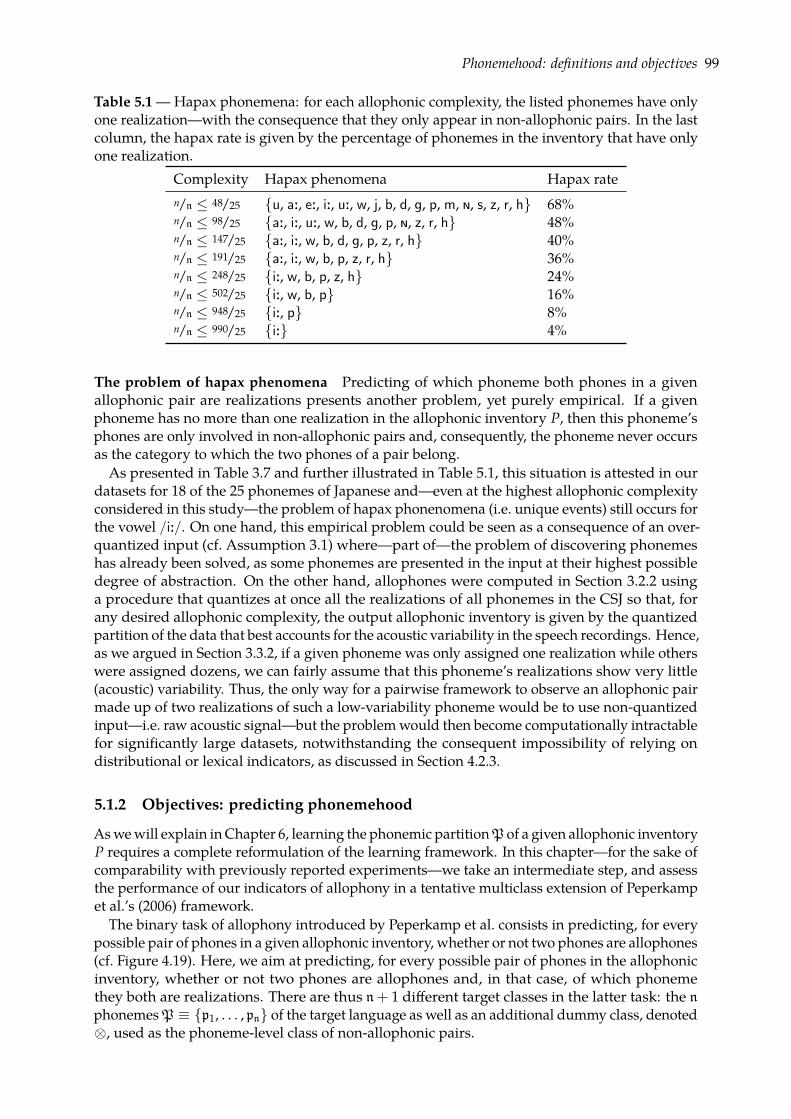
Phonemehood: definitions and objectives 99
Table 5.1 — Hapax phonemena: for each allophonic complexity, the listed phonemes have onlyone realization—with the consequence that they only appear in non-allophonic pairs. In the lastcolumn, the hapax rate is given by the percentage of phonemes in the inventory that have onlyone realization.
Complexity Hapax phenomena Hapax raten/n ≤ 48/25 u, a:, e:, i:, u:, w, j, b, d, g, p, m, ð, s, z, r, h 68%n/n ≤ 98/25 a:, i:, u:, w, b, d, g, p, ð, z, r, h 48%n/n ≤ 147/25 a:, i:, w, b, d, g, p, z, r, h 40%n/n ≤ 191/25 a:, i:, w, b, p, z, r, h 36%n/n ≤ 248/25 i:, w, b, p, z, h 24%n/n ≤ 502/25 i:, w, b, p 16%n/n ≤ 948/25 i:, p 8%n/n ≤ 990/25 i: 4%
The problem of hapax phenomena Predicting of which phoneme both phones in a givenallophonic pair are realizations presents another problem, yet purely empirical. If a givenphoneme has no more than one realization in the allophonic inventory P, then this phoneme’sphones are only involved in non-allophonic pairs and, consequently, the phoneme never occursas the category to which the two phones of a pair belong.As presented in Table 3.7 and further illustrated in Table 5.1, this situation is attested in our
datasets for 18 of the 25 phonemes of Japanese and—even at the highest allophonic complexityconsidered in this study—the problem of hapax phonenomena (i.e. unique events) still occurs forthe vowel /i:/. On one hand, this empirical problem could be seen as a consequence of an over-quantized input (cf. Assumption 3.1) where—part of—the problem of discovering phonemeshas already been solved, as some phonemes are presented in the input at their highest possibledegree of abstraction. On the other hand, allophones were computed in Section 3.2.2 usinga procedure that quantizes at once all the realizations of all phonemes in the CSJ so that, forany desired allophonic complexity, the output allophonic inventory is given by the quantizedpartition of the data that best accounts for the acoustic variability in the speech recordings. Hence,as we argued in Section 3.3.2, if a given phoneme was only assigned one realization while otherswere assigned dozens, we can fairly assume that this phoneme’s realizations show very little(acoustic) variability. Thus, the only way for a pairwise framework to observe an allophonic pairmade up of two realizations of such a low-variability phoneme would be to use non-quantizedinput—i.e. raw acoustic signal—but the problemwould then become computationally intractablefor significantly large datasets, notwithstanding the consequent impossibility of relying ondistributional or lexical indicators, as discussed in Section 4.2.3.
5.1.2 Objectives: predicting phonemehood
Aswewill explain in Chapter 6, learning the phonemic partitionP of a given allophonic inventoryP requires a complete reformulation of the learning framework. In this chapter—for the sake ofcomparability with previously reported experiments—we take an intermediate step, and assessthe performance of our indicators of allophony in a tentative multiclass extension of Peperkampet al.’s (2006) framework.
The binary task of allophony introduced by Peperkamp et al. consists in predicting, for everypossible pair of phones in a given allophonic inventory, whether or not two phones are allophones(cf. Figure 4.19). Here, we aim at predicting, for every possible pair of phones in the allophonicinventory, whether or not two phones are allophones and, in that case, of which phonemethey both are realizations. There are thus n+ 1 different target classes in the latter task: the nphonemesP ≡ p1, . . . , pn of the target language as well as an additional dummy class, denoted⊗, used as the phoneme-level class of non-allophonic pairs.
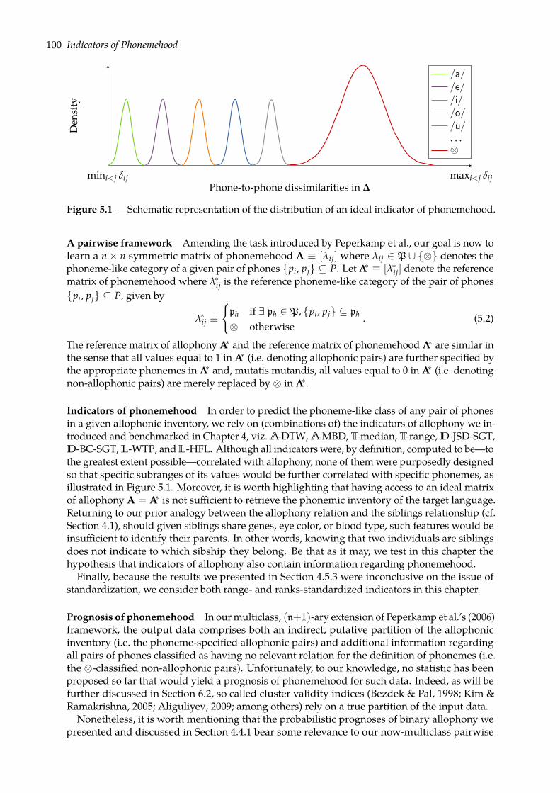
100 Indicators of Phonemehood
mini<j δij maxi<j δijPhone-to-phone dissimilarities in ∆
Den
sity
/a//e//i//o//u/. . .⊗
Figure 5.1— Schematic representation of the distribution of an ideal indicator of phonemehood.
A pairwise framework Amending the task introduced by Peperkamp et al., our goal is now tolearn a n× n symmetric matrix of phonemehood Λ ≡ [λij] where λij ∈ P ∪ ⊗ denotes thephoneme-like category of a given pair of phones pi, pj ⊆ P. Let Λ∗ ≡ [λ∗ij] denote the referencematrix of phonemehood where λ∗ij is the reference phoneme-like category of the pair of phonespi, pj ⊆ P, given by
λ∗ij ≡ph if ∃ ph ∈ P, pi, pj ⊆ ph
⊗ otherwise. (5.2)
The reference matrix of allophony A∗ and the reference matrix of phonemehood Λ∗ are similar inthe sense that all values equal to 1 in A∗ (i.e. denoting allophonic pairs) are further specified bythe appropriate phonemes in Λ∗ and, mutatis mutandis, all values equal to 0 in A∗ (i.e. denotingnon-allophonic pairs) are merely replaced by ⊗ in Λ∗.
Indicators of phonemehood In order to predict the phoneme-like class of any pair of phonesin a given allophonic inventory, we rely on (combinations of) the indicators of allophony we in-troduced and benchmarked in Chapter 4, viz. A-DTW, A-MBD, T-median, T-range, D-JSD-SGT,D-BC-SGT, L-WTP, and L-HFL. Although all indicators were, by definition, computed to be—tothe greatest extent possible—correlated with allophony, none of themwere purposedly designedso that specific subranges of its values would be further correlated with specific phonemes, asillustrated in Figure 5.1. Moreover, it is worth highlighting that having access to an ideal matrixof allophony A = A∗ is not sufficient to retrieve the phonemic inventory of the target language.Returning to our prior analogy between the allophony relation and the siblings relationship (cf.Section 4.1), should given siblings share genes, eye color, or blood type, such features would beinsufficient to identify their parents. In other words, knowing that two individuals are siblingsdoes not indicate to which sibship they belong. Be that as it may, we test in this chapter thehypothesis that indicators of allophony also contain information regarding phonemehood.Finally, because the results we presented in Section 4.5.3 were inconclusive on the issue of
standardization, we consider both range- and ranks-standardized indicators in this chapter.
Prognosis of phonemehood In ourmulticlass, (n+1)-ary extension of Peperkamp et al.’s (2006)framework, the output data comprises both an indirect, putative partition of the allophonicinventory (i.e. the phoneme-specified allophonic pairs) and additional information regardingall pairs of phones classified as having no relevant relation for the definition of phonemes (i.e.the ⊗-classified non-allophonic pairs). Unfortunately, to our knowledge, no statistic has beenproposed so far that would yield a prognosis of phonemehood for such data. Indeed, as will befurther discussed in Section 6.2, so called cluster validity indices (Bezdek & Pal, 1998; Kim &Ramakrishna, 2005; Aliguliyev, 2009; among others) rely on a true partition of the input data.Nonetheless, it is worth mentioning that the probabilistic prognoses of binary allophony we
presented and discussed in Section 4.4.1 bear some relevance to our now-multiclass pairwise
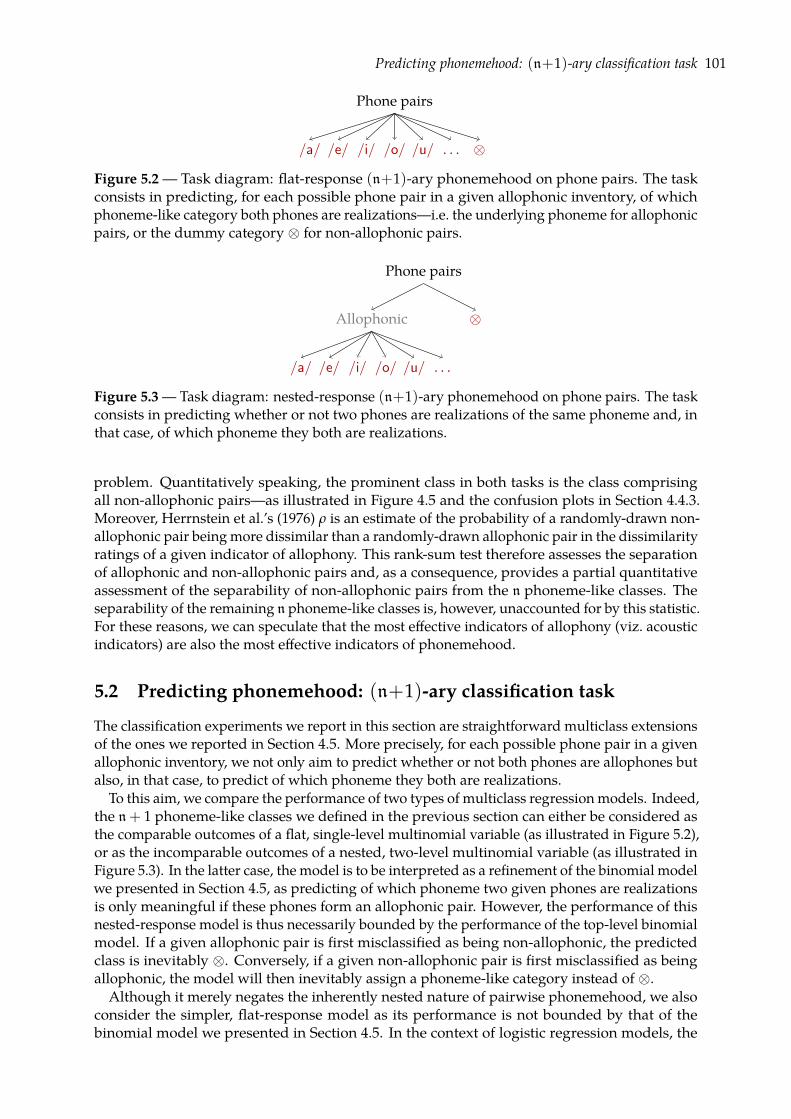
Predicting phonemehood: (n+1)-ary classification task 101
Phone pairs
/a/ /e/ /i/ /o/ /u/ . . . ⊗
Figure 5.2 — Task diagram: flat-response (n+1)-ary phonemehood on phone pairs. The taskconsists in predicting, for each possible phone pair in a given allophonic inventory, of whichphoneme-like category both phones are realizations—i.e. the underlying phoneme for allophonicpairs, or the dummy category ⊗ for non-allophonic pairs.
Phone pairs
Allophonic
/a/ /e/ /i/ /o/ /u/ . . .
⊗
Figure 5.3— Task diagram: nested-response (n+1)-ary phonemehood on phone pairs. The taskconsists in predicting whether or not two phones are realizations of the same phoneme and, inthat case, of which phoneme they both are realizations.
problem. Quantitatively speaking, the prominent class in both tasks is the class comprisingall non-allophonic pairs—as illustrated in Figure 4.5 and the confusion plots in Section 4.4.3.Moreover, Herrnstein et al.’s (1976) ρ is an estimate of the probability of a randomly-drawn non-allophonic pair beingmore dissimilar than a randomly-drawn allophonic pair in the dissimilarityratings of a given indicator of allophony. This rank-sum test therefore assesses the separationof allophonic and non-allophonic pairs and, as a consequence, provides a partial quantitativeassessment of the separability of non-allophonic pairs from the n phoneme-like classes. Theseparability of the remaining n phoneme-like classes is, however, unaccounted for by this statistic.For these reasons, we can speculate that the most effective indicators of allophony (viz. acousticindicators) are also the most effective indicators of phonemehood.
5.2 Predicting phonemehood: (n+1)-ary classification task
The classification experiments we report in this section are straightforward multiclass extensionsof the ones we reported in Section 4.5. More precisely, for each possible phone pair in a givenallophonic inventory, we not only aim to predict whether or not both phones are allophones butalso, in that case, to predict of which phoneme they both are realizations.
To this aim, we compare the performance of two types of multiclass regression models. Indeed,the n+ 1 phoneme-like classes we defined in the previous section can either be considered asthe comparable outcomes of a flat, single-level multinomial variable (as illustrated in Figure 5.2),or as the incomparable outcomes of a nested, two-level multinomial variable (as illustrated inFigure 5.3). In the latter case, the model is to be interpreted as a refinement of the binomial modelwe presented in Section 4.5, as predicting of which phoneme two given phones are realizationsis only meaningful if these phones form an allophonic pair. However, the performance of thisnested-response model is thus necessarily bounded by the performance of the top-level binomialmodel. If a given allophonic pair is first misclassified as being non-allophonic, the predictedclass is inevitably ⊗. Conversely, if a given non-allophonic pair is first misclassified as beingallophonic, the model will then inevitably assign a phoneme-like category instead of ⊗.Although it merely negates the inherently nested nature of pairwise phonemehood, we also
consider the simpler, flat-response model as its performance is not bounded by that of thebinomial model we presented in Section 4.5. In the context of logistic regression models, the
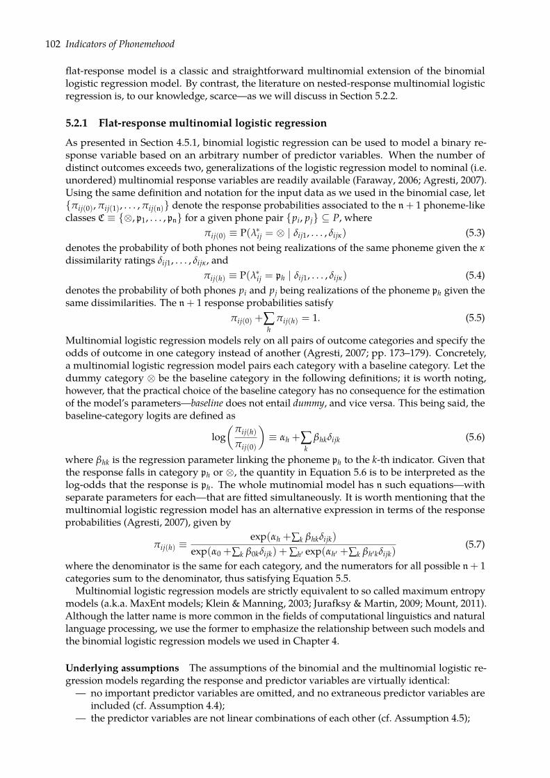
102 Indicators of Phonemehood
flat-response model is a classic and straightforward multinomial extension of the binomiallogistic regression model. By contrast, the literature on nested-response multinomial logisticregression is, to our knowledge, scarce—as we will discuss in Section 5.2.2.
5.2.1 Flat-response multinomial logistic regression
As presented in Section 4.5.1, binomial logistic regression can be used to model a binary re-sponse variable based on an arbitrary number of predictor variables. When the number ofdistinct outcomes exceeds two, generalizations of the logistic regression model to nominal (i.e.unordered) multinomial response variables are readily available (Faraway, 2006; Agresti, 2007).Using the same definition and notation for the input data as we used in the binomial case, letπij(0), πij(1), . . . , πij(n) denote the response probabilities associated to the n+ 1 phoneme-likeclasses C ≡ ⊗, p1, . . . , pn for a given phone pair pi, pj ⊆ P, where
πij(0) ≡ P(λ∗ij = ⊗ | δij1, . . . , δijκ) (5.3)denotes the probability of both phones not being realizations of the same phoneme given the κdissimilarity ratings δij1, . . . , δijκ, and
πij(h) ≡ P(λ∗ij = ph | δij1, . . . , δijκ) (5.4)denotes the probability of both phones pi and pj being realizations of the phoneme ph given thesame dissimilarities. The n+ 1 response probabilities satisfy
πij(0) +∑h
πij(h) = 1. (5.5)
Multinomial logistic regression models rely on all pairs of outcome categories and specify theodds of outcome in one category instead of another (Agresti, 2007; pp. 173–179). Concretely,a multinomial logistic regression model pairs each category with a baseline category. Let thedummy category ⊗ be the baseline category in the following definitions; it is worth noting,however, that the practical choice of the baseline category has no consequence for the estimationof the model’s parameters—baseline does not entail dummy, and vice versa. This being said, thebaseline-category logits are defined as
log(
πij(h)
πij(0)
)≡ αh +∑
kβhkδijk (5.6)
where βhk is the regression parameter linking the phoneme ph to the k-th indicator. Given thatthe response falls in category ph or ⊗, the quantity in Equation 5.6 is to be interpreted as thelog-odds that the response is ph. The whole mutinomial model has n such equations—withseparate parameters for each—that are fitted simultaneously. It is worth mentioning that themultinomial logistic regression model has an alternative expression in terms of the responseprobabilities (Agresti, 2007), given by
πij(h) ≡exp(αh +∑k βhkδijk)
exp(α0 +∑k β0kδijk) + ∑h′ exp(αh′ +∑k βh′kδijk)(5.7)
where the denominator is the same for each category, and the numerators for all possible n+ 1categories sum to the denominator, thus satisfying Equation 5.5.Multinomial logistic regression models are strictly equivalent to so called maximum entropy
models (a.k.a. MaxEnt models; Klein & Manning, 2003; Jurafksy & Martin, 2009; Mount, 2011).Although the latter name is more common in the fields of computational linguistics and naturallanguage processing, we use the former to emphasize the relationship between such models andthe binomial logistic regression models we used in Chapter 4.
Underlying assumptions The assumptions of the binomial and the multinomial logistic re-gression models regarding the response and predictor variables are virtually identical:— no important predictor variables are omitted, and no extraneous predictor variables are
included (cf. Assumption 4.4);— the predictor variables are not linear combinations of each other (cf. Assumption 4.5);
Predicting phonemehood: (n+1)-ary classification task 103
— the predictor variables are measured without error (cf. Assumption 4.6).The last two assumptions, however, need to be amended in order to account for the specificformulation of the multinomial model:
Assumption 5.1 The true outcome probabilities follow a multinomial distribution. Thereby, theobservations are independent, meaning that the outcome for a given observation does not affectthe outcome for another (cf. Assumption 4.2).
Assumption 5.2 The log-odds of the true outcomes against the baseline category are a functionof a (weighted) linear combination of the predictor variables (cf. Assumption 4.3).
We consider that the arguments we presented in Section 4.5.1 regarding the validity of theseassumptions in the binomial case also hold in the multinomial case.
Model-fitting Fitting a multinomial logistic regression model consists in estimating the nκregression parameters β11, . . . , βnκ as well as the n intercepts α1, . . . , αn. As in the case of binomiallogistic regression models, the estimation process relies on a given set of training observationsof the form 〈δij1, . . . , δijκ, wij, λ∗ij〉, i.e. comprising the dissimilarity ratings assigned to a givenphone pair pi, pj ∈ P, its weight, and its true phoneme-like category. The numerical algorithmwe used in these experiments outputs the n(κ + 1) values that maximize the likelihood of theparameters given the training data (Agresti, 2007; Venables & Ripley, 2002; cf. nnet::multinom).
Finally, for the sake of comparability with the experiments reported in Section 4.5, we reiterateour argument about the relevance of confirmatory overfitting and, accordingly, trained andtested all multinomial logistic regression models using all available data.
Predictions For the purpose of classifying all possible phone pairs in a given allophonic inven-tory P, the predicted phoneme-like category λij of a given pair pi, pj ⊆ P is simply defined asthe most probable one, i.e.
λij ≡ cτ where τ ≡ arg maxτ∈(0,1,...,n) πij(τ) (5.8)denotes the index of the most probable phoneme-like category.
5.2.2 Nested-response multinomial logistic regression
In the case of pairwise phonemehood, the phoneme-like outcomes form an intrinsically nestedvariable: the model first needs to determine whether two given phones are allophones and—inthat case, and only in that case—of which phoneme they both are realizations. Whereas thereis a considerable literature describing logistic regression models whose predictor variables arestructured (a.k.a. hierarchical, random-effects, andmixed-effectsmodels; Agresti, 2007; Gelman&Hill, 2007), logistic regression models whose response variable is structured are, to our knowledge,only (briefly) discussed by McCullagh & Nelder (1989; pp. 160–164), Faraway (2006; pp. 113–117),and Rodríguez (2007; ch. 6, pp. 11–15).Our methodology for such nested-response models follows Faraway’s analysis of the dataset
collected by Lowe et al. (1971) concerning live births with deformations of the central nervoussystem. Though completely unrelated, this dataset indeed shares many properties with thedata at hand in the present study: live births (pairs of phones) can occur with or withoutdeformations of the central nervous system (can be allophonic or not) and, in that case, variousdeformations (phonemes) are possible. Moreover, in both datasets, the outcome of lesser interest(no deformation and no allophony) numerically dominates all other possible outcomes.
Following Faraway (2006), we separately develop a binomial model for allophony and amultinomial model for phonemehood. Let
πij ≡ P(λ∗ij 6= ⊗ | δij1, . . . , δijκ) (5.9)
104 Indicators of Phonemehood
denote the conditional probability of the pair of phones pi, pj ⊆ P being allophonic giventhe κ predictor values δij1, . . . , δijκ. As discussed in Section 4.5.1, the top-level binomial logisticregression model has linear form for the logit of the probability of allophony, i.e.
logit(πij) ≡ α +κ
∑k=1
βkδijk. (5.10)
Furthermore, let πij(1), . . . , πij(n) denote the response probabilities associated to the nphonemicclasses P ≡ p1, . . . , pn for a given allophonic pair of phones pi, pj ⊆ P, where
πij(h) ≡ P(λ∗ij = ph | δij1, . . . , δijκ, λ∗ij 6= ⊗) (5.11)denotes the probability of both phones pi and pj being realizations of the phoneme ph given thesame dissimilarities. The n+ 1 response probabilities satisfy
∑h
πij(h) = 1 (5.12)
and, as presented in the previous section, the low-level multinomial logistic regression model asthe following expression in terms of the response probabilities:
πij(h) ≡exp(α′h +∑k β′hkδijk)
∑h′ exp(α′h′ +∑k β′h′kδijk). (5.13)
Finally, as emphasized by McCullagh & Nelder (1989), it is worth noting thatThere is no good reason here to expect that the coefficients [α, β1, . . . , βκ, and α′1, . . . , α′n,β′11, . . . , βnκ] might be equal or even comparable.~
Predictions For the purpose of classifying all possible phone pairs in a given allophonic inven-tory P, the predicted phoneme-like category λij of a given pair pi, pj ⊆ P is given by
λij ≡⊗ if πij ≤ .5ph otherwise, where h ≡ arg maxh πij(h)
(5.14)
denotes the index of the most probable phoneme for the pair of phones pi, pj.
5.2.3 Evaluation
In these experiments, as in the oneswe presented in Section 4.5, we are interested in the predictivepower of the regression models.
Goodness of fit The first quantitative criterion we use to assess the fit of a given multinomiallogistic regression model to the reference matrix of phonemehood Λ∗ is the aforementioned AIC.
The definition of the AIC in the flat-response multinomial case is a straightforward extensionof the definition given in Equation 4.45 for the binomial case: the AIC of a regression modelis a measure of the maximized likelihood of its parameters, penalized by the number of suchparameters. The only difference lies in the latter penalty: whereas a binomial logistic regressionmodel has κ + 1 parameters, a multinomial model has n(κ + 1) parameters.
To our knowledge, no extension of the definition of the AIC has yet been proposed for nested-response multinomial logistic regression models.
Contingency table The other two criteria we use to assess the performance of (combinationsof) indicators of phonemehood rely on an actual pairwise classification of their input into then+ 1 phoneme-like categories. These criteria are thus applicable to, and meaningful for, bothflat- and nested-response multinomial models. For each regression model, a contingency table isused to cross-classify the reference outcomes with the model’s predictions. In this multiclasssetup, this cross-classification yields a (n+1)× (n+1) contingency table. Let T ≡ [tτ′τ] denotesuch a contingency table where, by convention, τ denotes the index over reference classes and τ′
the index over predicted classes. The table is thus non-symmetric: while t0h denotes the numberof non-allophonic pairs that were misclassified as realizations of ph, th0 denotes the number of
Predicting phonemehood: (n+1)-ary classification task 105
realizations of ph that were misclassified as non-allophonic pairs. In each cell, the non-negativecount tτ′τ is given by
tτ′τ ≡∑i<j
wijJλ∗ij = cτ′KJλij = cτK. (5.15)
Pairwise evaluation The evaluation measures we defined in Section 4.5.2—viz. precision,recall, F-score, and MCC—are only appropriate when there are exactly two possible outcomes.Multiclass predictions can however be considered as a series of pairwise decisions, one for eachpair of observations in the test data (Manning et al., 2008). In that case, TP denotes the (weighted)number of pairs of observations of equal class that were classified as belonging to the same class,TN the number of pairs of observations of different classes that were classified as belonging todifferent classes, FP the number of pairs of observations of different classes that were classifiedas belonging to the same class, and FN the number of observations of equal class that wereclassified as belonging to different classes.Because our elementary observations consist in pairs of phones, such a pairwise evaluation
actually involves comparing the predictions for all pairs of pairs of phones. For a given allophonicinventory and a given regression model, computing the 2× 2 pairwise contingency table thusrequires O(n4) operations and, hence, becomes computationally intractable as the allophoniccomplexity of the input increases—especially considering the fact that this computation needsto be repeated for 24 different regression models, and 20 allophonic inventories.
Global accuracy Various evaluationmeasures can however be computed from a (n+1)× (n+1)contingency table. The first measure on which we rely is the global accuracy of the predictions,that is to say the average number of correct predictions across all phoneme-like classes. Formally,global accuracy is given by
accuracy(Λ, Λ∗) ≡ P(λij = λ∗ij) u∑τ tττ
∑τ ∑τ′ tτ′τ=
∑i<j wijJλij = λ∗ijK
∑i<j wij. (5.16)
In the manner of the pairwise accuracy presented in Section 4.5.2, the global multiclass accuracycan receive a probabilistic interpretation: it is an estimate of the probability P(λij = λ∗ij) ofthe predicted class λij of a randomly-drawn pair of phones pi, pj ⊆ P being equal to itsreference phoneme-like class λ∗ij. As far as the contingency table is concerned, a perfectlyaccurate classification Λ = Λ∗ would result in a strictly diagonal contingency table T. By contrast,the more off-diagonal observations, the less accurate the classification.
Classwise accuracy The second evaluation measure we rely on in these experiments is knownas classwise accuracy. For a given phoneme-like class cτ ∈ C, its classwise accuracy is an estimateof the probability P(λij = cτ | λ∗ij = cτ) of a randomly-drawn pair of phones pi, pj ⊆ P whosereference class is cτ being actually classified as cτ. Formally, classwise accuracy is given by
accuracy(cτ, Λ, Λ∗) ≡ P(λij = cτ | λ∗ij = cτ) utττ
∑τ′ tττ′=
∑i<j wijJλij = λ∗ij = cτK
∑i<j wijJλ∗ij = cτK. (5.17)
Whereas global accuracy aggregates all correct predictions—regardless of the predicted class—classwise accuracy allows for a fine-grained exploration of the performance of a multinomiallogistic regression model. For instance, we observed in Chapter 4 that the high performance ofbinomial logistic regression models was mainly due to the correct rejection of non-allophonicpairs. We can thus speculate that the global accuracy of any multinomial model’s predictionswill benefit from these correct rejections. Comparing the classwise accuracy of⊗ to the classwiseaccuracies of other phoneme-like categories will thus allow us to assess whether or not indicatorsof allophony are also indicators of phonemehood.
106 Indicators of Phonemehood
5.2.4 Results
The performance of all flat-response multinomial logistic regression models is presented in Fig-ure 5.4, Figure 5.6, Figure 5.5 and Table 5.2. The performance of all nested-response multinomiallogistic regression models is presented in Figure 5.6 and Table 5.3.
Goodness of fit Let us first consider the goodness of fit tests reported in Figure 5.4 for flat-response models. First, it is worth mentioning that this figure resembles the plot of the AICof binomial logistic regression models in Figure 4.21. Indeed, as we observed for binomialmodels, all flat-response models’ AIC increases with the allophonic complexity of their input,meaning that the more phonemes have allophones, the less a multinomial logistic regressionmodel is able to fit the phoneme-like partition of all possible pairs of phones. Moreover, acousticindicators appear to be, once again, the individual indicators that yield regression models withthe best fit, as well as the indicators whose AIC gives approximate bounds on that of the quartetmodels. However, it appears that combining indicators is—on average—nomore interesting thanonly using the acoustic indicator A-DTW. Finally, individual flat-response models relying ontemporal, distributional, and lexical indicators are indistinguishable, as far as AIC is concerned.However, the goodness of fit tests reported in Figure 5.4 depart from the ones in Figure 4.21
on two main points. First, is it worth noting that the AIC of multinomial models increases fasterthan that of binomial models. Consider, for example, the AIC values at the maximal allophoniccomplexity of 990/25 allophones per phoneme: whereas the AIC of individual binomial modelsis approximately equal to 35× 104, the AIC of individual multinomial models is greater than50× 104. While, to our knowledge, AIC values are not to be interpreted in isolation, a comparisonof both values at 990/25 allophones per phoneme suffice to show that logistic regression yieldsmodels with a fit almost 1.5 times better in the binomial case than in the flat-responsemultinomialcase.
Range or ranks? In the previous chapter, the results presented in Figures 4.27 and 4.28 wereinconclusive on the issue of standardization, i.e. assessing whether allophony can be learnedfrom a mere ranking of a given indicator’s values, or if the values themselves convey relevantinformation. To this aim, our methodology has consisted in examining the difference in AICbetween pairs of models trained with the same (combination of) indicators, but where one wastrained with range-standardized indicators and the other was trained with ranks-standardizedindicators. A negative difference indicates that the AIC observed on range-standardized indi-cators is lesser than the AIC observed on ranks-standardized indicators. Because the AIC is tobe minimized, a negative difference indicates that relying on indicators’ absolute values yieldsmodels with a better fit than relying on mere rankings of each indicator’s values or—to saythe least—that the (n+1)-ary phoneme-like classification of all phone pairs is more accuratelymodeled by a linear combination of values than by a linear combination of ranks.
As illustrated in Figure 5.5, a clear pattern emerges for multinomial logistic regression modelsfrom 300/25 allophones per phoneme onwards. Whereas individual models appear to be ratherinsensitive to the particular standardization technique used on the indicators (cf. Figure 4.28),we observe significant negative differences between the AIC of range- and ranks-standardizedindicators for all quartet models. Moreover, these differences tend to increase with the allophoniccomplexity of the input. Therefore, phonemehood appears to be better modeled by the truephone-to-phone dissimilarity ratings collected in each indicator of allophony than by the rankingthese values denote. This result is important in itself, as the evaluation of various studies buildingupon Peperkamp et al.’s (2006) framework was limited to the computation of Herrnstein et al.’s(1976) rank-sum test (Martin et al., 2009; Dautriche, 2009; Boruta, 2009, 2011b). Notwithstandingour prior theoretical argument that ρ is at best a prognosis of allophony—rather than a trueevaluation measure, cf. Section 4.4.1—we consider the results presented in Figure 5.5 to beempirical evidence against a mere examination of the ranking of phone pairs underlying each
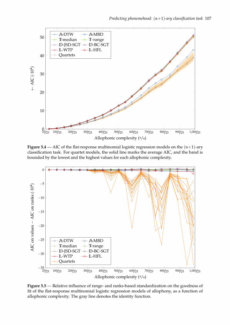
Predicting phonemehood: (n+1)-ary classification task 107
100/25 200/25 300/25 400/25 500/25 600/25 700/25 800/25 900/25 1,000/250
10
20
30
40
50
25/25
Allophonic complexity (n/n)
←A
IC(·1
04 )A-DTW A-MBDT-median T-rangeD-JSD-SGT D-BC-SGTL-WTP L-HFLQuartets
Figure 5.4 — AIC of the flat-response multinomial logistic regression models on the (n+1)-aryclassification task. For quartet models, the solid line marks the average AIC, and the band isbounded by the lowest and the highest values for each allophonic complexity.
100/25 200/25 300/25 400/25 500/25 600/25 700/25 800/25 900/25 1,000/25−35
−30
−25
−20
−15
−10
−5
0
25/25
Allophonic complexity (n/n)
AIC
onva
lues−
AIC
onra
nks(·10
4 )
A-DTW A-MBDT-median T-rangeD-JSD-SGT D-BC-SGTL-WTP L-HFLQuartets
Figure 5.5—Relative influence of range- and ranks-based standardization on the goodness offit of the flat-response multinomial logistic regression models of allophony, as a function ofallophonic complexity. The gray line denotes the identity function.
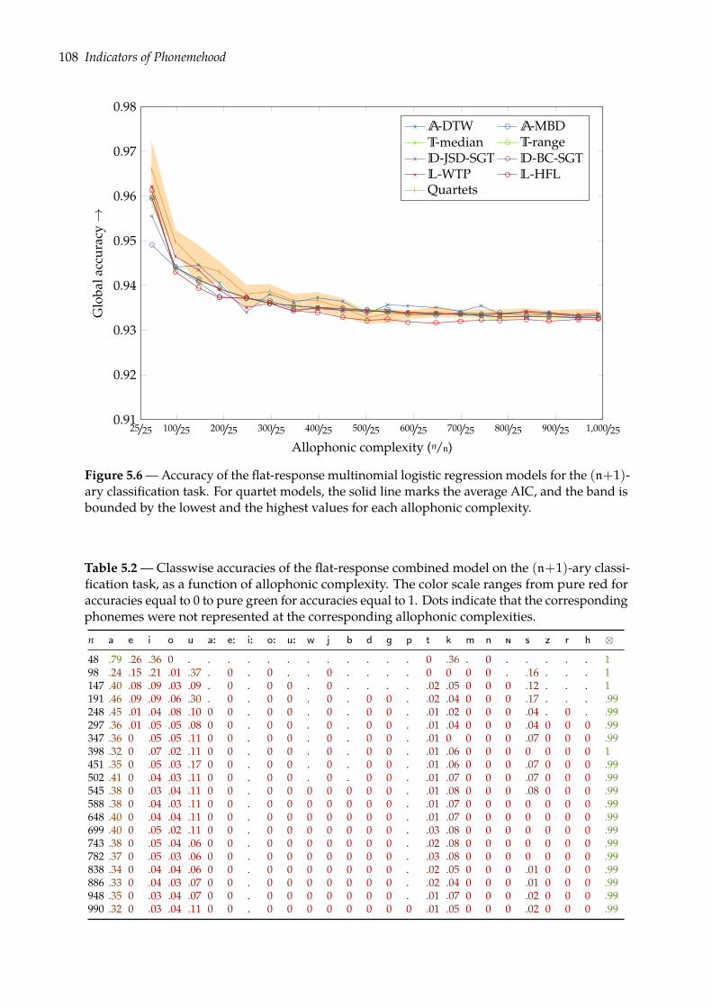
108 Indicators of Phonemehood
100/25 200/25 300/25 400/25 500/25 600/25 700/25 800/25 900/25 1,000/250.91
0.92
0.93
0.94
0.95
0.96
0.97
0.98
25/25
Allophonic complexity (n/n)
Glo
bala
ccur
acy→
A-DTW A-MBDT-median T-rangeD-JSD-SGT D-BC-SGTL-WTP L-HFLQuartets
Figure 5.6—Accuracy of the flat-response multinomial logistic regression models for the (n+1)-ary classification task. For quartet models, the solid line marks the average AIC, and the band isbounded by the lowest and the highest values for each allophonic complexity.
Table 5.2—Classwise accuracies of the flat-response combined model on the (n+1)-ary classi-fication task, as a function of allophonic complexity. The color scale ranges from pure red foraccuracies equal to 0 to pure green for accuracies equal to 1. Dots indicate that the correspondingphonemes were not represented at the corresponding allophonic complexities.n a e i o u a: e: i: o: u: w j b d g p t k m n ð s z r h ⊗48 .79 .26 .36 0 . . . . . . . . . . . . 0 .36 . 0 . . . . . 198 .24 .15 .21 .01 .37 . 0 . 0 . . 0 . . . . 0 0 0 0 . .16 . . . 1147 .40 .08 .09 .03 .09 . 0 . 0 0 . 0 . . . . .02 .05 0 0 0 .12 . . . 1191 .46 .09 .09 .06 .30 . 0 . 0 0 . 0 . 0 0 . .02 .04 0 0 0 .17 . . . .99248 .45 .01 .04 .08 .10 0 0 . 0 0 . 0 . 0 0 . .01 .02 0 0 0 .04 . 0 . .99297 .36 .01 .05 .05 .08 0 0 . 0 0 . 0 . 0 0 . .01 .04 0 0 0 .04 0 0 0 .99347 .36 0 .05 .05 .11 0 0 . 0 0 . 0 . 0 0 . .01 0 0 0 0 .07 0 0 0 .99398 .32 0 .07 .02 .11 0 0 . 0 0 . 0 . 0 0 . .01 .06 0 0 0 0 0 0 0 1451 .35 0 .05 .03 .17 0 0 . 0 0 . 0 . 0 0 . .01 .06 0 0 0 .07 0 0 0 .99502 .41 0 .04 .03 .11 0 0 . 0 0 . 0 . 0 0 . .01 .07 0 0 0 .07 0 0 0 .99545 .38 0 .03 .04 .11 0 0 . 0 0 0 0 0 0 0 . .01 .08 0 0 0 .08 0 0 0 .99588 .38 0 .04 .03 .11 0 0 . 0 0 0 0 0 0 0 . .01 .07 0 0 0 0 0 0 0 .99648 .40 0 .04 .04 .11 0 0 . 0 0 0 0 0 0 0 . .01 .07 0 0 0 0 0 0 0 .99699 .40 0 .05 .02 .11 0 0 . 0 0 0 0 0 0 0 . .03 .08 0 0 0 0 0 0 0 .99743 .38 0 .05 .04 .06 0 0 . 0 0 0 0 0 0 0 . .02 .08 0 0 0 0 0 0 0 .99782 .37 0 .05 .03 .06 0 0 . 0 0 0 0 0 0 0 . .03 .08 0 0 0 0 0 0 0 .99838 .34 0 .04 .04 .06 0 0 . 0 0 0 0 0 0 0 . .02 .05 0 0 0 .01 0 0 0 .99886 .33 0 .04 .03 .07 0 0 . 0 0 0 0 0 0 0 . .02 .04 0 0 0 .01 0 0 0 .99948 .35 0 .03 .04 .07 0 0 . 0 0 0 0 0 0 0 . .01 .07 0 0 0 .02 0 0 0 .99990 .32 0 .03 .04 .11 0 0 . 0 0 0 0 0 0 0 0 .01 .05 0 0 0 .02 0 0 0 .99
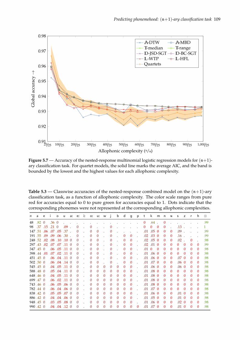
Predicting phonemehood: (n+1)-ary classification task 109
100/25 200/25 300/25 400/25 500/25 600/25 700/25 800/25 900/25 1,000/250.91
0.92
0.93
0.94
0.95
0.96
0.97
0.98
25/25
Allophonic complexity (n/n)
Glo
bala
ccur
acy→
A-DTW A-MBDT-median T-rangeD-JSD-SGT D-BC-SGTL-WTP L-HFLQuartets
Figure 5.7 —Accuracy of the nested-response multinomial logistic regression models for (n+1)-ary classification task. For quartet models, the solid line marks the average AIC, and the band isbounded by the lowest and the highest values for each allophonic complexity.
Table 5.3 — Classwise accuracies of the nested-response combined model on the (n+1)-aryclassification task, as a function of allophonic complexity. The color scale ranges from purered for accuracies equal to 0 to pure green for accuracies equal to 1. Dots indicate that thecorresponding phonemes were not represented at the corresponding allophonic complexities.n a e i o u a: e: i: o: u: w j b d g p t k m n ð s z r h ⊗48 .82 0 .36 0 . . . . . . . . . . . . 0 .64 . 0 . . . . . .9998 .37 .15 .21 0 .09 . 0 . 0 . . 0 . . . . 0 0 0 0 . .13 . . . 1147 .51 .06 .07 .05 .37 . 0 . 0 0 . 0 . . . . .01 .05 0 0 0 .09 . . . .99191 .55 .09 .09 .06 .30 . 0 . 0 0 . 0 . 0 0 . .02 .03 0 0 0 .16 . . . .99248 .52 .02 .08 .10 .10 0 0 . 0 0 . 0 . 0 0 . .02 .05 0 0 0 .02 . 0 . .98297 .43 .02 .07 .07 .11 0 0 . 0 0 . 0 . 0 0 . .02 .01 0 0 0 0 0 0 0 .99347 .45 0 .06 .05 .11 0 0 . 0 0 . 0 . 0 0 . .01 0 0 0 0 0 0 0 0 .98398 .44 .01 .07 .02 .11 0 0 . 0 0 . 0 . 0 0 . .01 .06 0 0 0 0 0 0 0 .98451 .45 0 .06 .04 .11 0 0 . 0 0 . 0 . 0 0 . .01 .06 0 0 0 .07 0 0 0 .98502 .50 0 .06 .04 .14 0 0 . 0 0 . 0 . 0 0 . .01 .07 0 0 0 .06 0 0 0 .98545 .45 0 .04 .05 .11 0 0 . 0 0 0 0 0 0 0 . .01 .06 0 0 0 .06 0 0 0 .98588 .48 0 .05 .04 .11 0 0 . 0 0 0 0 0 0 0 . .01 .08 0 0 0 0 0 0 0 .98648 .46 0 .04 .05 .11 0 0 . 0 0 0 0 0 0 0 . .01 .08 0 0 0 0 0 0 0 .98699 .47 0 .06 .02 .11 0 0 . 0 0 0 0 0 0 0 . .01 .08 0 0 0 0 0 0 0 .98743 .46 0 .06 .05 .06 0 0 . 0 0 0 0 0 0 0 . .01 .08 0 0 0 0 0 0 0 .98782 .44 0 .06 .04 .06 0 0 . 0 0 0 0 0 0 0 . .01 .07 0 0 0 0 0 0 0 .98838 .42 0 .05 .05 .07 0 0 . 0 0 0 0 0 0 0 . .01 .06 0 0 0 .01 0 0 0 .98886 .42 0 .04 .04 .06 0 0 . 0 0 0 0 0 0 0 . .01 .05 0 0 0 .01 0 0 0 .98948 .45 0 .03 .05 .08 0 0 . 0 0 0 0 0 0 0 . .01 .06 0 0 0 .02 0 0 0 .98990 .42 0 .04 .04 .12 0 0 . 0 0 0 0 0 0 0 0 .01 .07 0 0 0 .01 0 0 0 .98
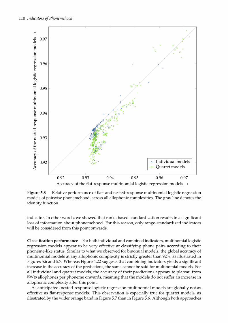
110 Indicators of Phonemehood
0.92 0.93 0.94 0.95 0.96 0.97
0.92
0.93
0.94
0.95
0.96
0.97
Accuracy of the flat-response multinomial logistic regression models→
Accuracyof
thene
sted
-respo
nsemultin
omiallog
istic
regression
mod
els→
Individual modelsQuartet models
Figure 5.8— Relative performance of flat- and nested-response multinomial logistic regressionmodels of pairwise phonemehood, across all allophonic complexities. The gray line denotes theidentity function.
indicator. In other words, we showed that ranks-based standardization results in a significantloss of information about phonemehood. For this reason, only range-standardized indicatorswill be considered from this point onwards.
Classification performance For both individual and combined indicators, multinomial logisticregression models appear to be very effective at classifying phone pairs according to theirphoneme-like status. Similar to what we observed for binomial models, the global accuracy ofmultinomial models at any allophonic complexity is strictly greater than 92%, as illustrated inFigures 5.6 and 5.7. Whereas Figure 4.22 suggests that combining indicators yields a significantincrease in the accuracy of the predictions, the same cannot be said for multinomial models. Forall individual and quartet models, the accuracy of their predictions appears to plateau from500/25 allophones per phoneme onwards, meaning that the models do not suffer an increase inallophonic complexity after this point.As anticipated, nested-response logistic regression multinomial models are globally not as
effective as flat-response models. This observation is especially true for quartet models, asillustrated by the wider orange band in Figure 5.7 than in Figure 5.6. Although both approaches
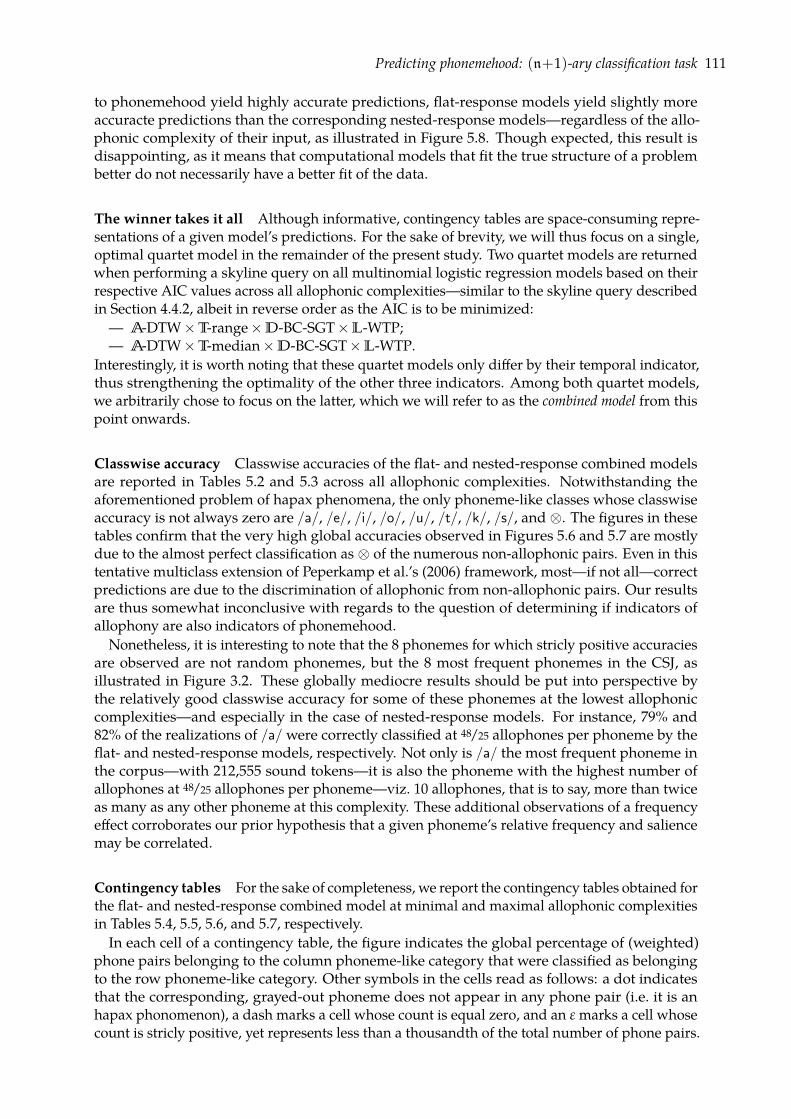
Predicting phonemehood: (n+1)-ary classification task 111
to phonemehood yield highly accurate predictions, flat-response models yield slightly moreaccuracte predictions than the corresponding nested-response models—regardless of the allo-phonic complexity of their input, as illustrated in Figure 5.8. Though expected, this result isdisappointing, as it means that computational models that fit the true structure of a problembetter do not necessarily have a better fit of the data.
The winner takes it all Although informative, contingency tables are space-consuming repre-sentations of a given model’s predictions. For the sake of brevity, we will thus focus on a single,optimal quartet model in the remainder of the present study. Two quartet models are returnedwhen performing a skyline query on all multinomial logistic regression models based on theirrespective AIC values across all allophonic complexities—similar to the skyline query describedin Section 4.4.2, albeit in reverse order as the AIC is to be minimized:— A-DTW×T-range×D-BC-SGT×L-WTP;— A-DTW×T-median×D-BC-SGT×L-WTP.
Interestingly, it is worth noting that these quartet models only differ by their temporal indicator,thus strengthening the optimality of the other three indicators. Among both quartet models,we arbitrarily chose to focus on the latter, which we will refer to as the combined model from thispoint onwards.
Classwise accuracy Classwise accuracies of the flat- and nested-response combined modelsare reported in Tables 5.2 and 5.3 across all allophonic complexities. Notwithstanding theaforementioned problem of hapax phenomena, the only phoneme-like classes whose classwiseaccuracy is not always zero are /a/, /e/, /i/, /o/, /u/, /t/, /k/, /s/, and ⊗. The figures in thesetables confirm that the very high global accuracies observed in Figures 5.6 and 5.7 are mostlydue to the almost perfect classification as ⊗ of the numerous non-allophonic pairs. Even in thistentative multiclass extension of Peperkamp et al.’s (2006) framework, most—if not all—correctpredictions are due to the discrimination of allophonic from non-allophonic pairs. Our resultsare thus somewhat inconclusive with regards to the question of determining if indicators ofallophony are also indicators of phonemehood.
Nonetheless, it is interesting to note that the 8 phonemes for which stricly positive accuraciesare observed are not random phonemes, but the 8 most frequent phonemes in the CSJ, asillustrated in Figure 3.2. These globally mediocre results should be put into perspective bythe relatively good classwise accuracy for some of these phonemes at the lowest allophoniccomplexities—and especially in the case of nested-response models. For instance, 79% and82% of the realizations of /a/ were correctly classified at 48/25 allophones per phoneme by theflat- and nested-response models, respectively. Not only is /a/ the most frequent phoneme inthe corpus—with 212,555 sound tokens—it is also the phoneme with the highest number ofallophones at 48/25 allophones per phoneme—viz. 10 allophones, that is to say, more than twiceas many as any other phoneme at this complexity. These additional observations of a frequencyeffect corroborates our prior hypothesis that a given phoneme’s relative frequency and saliencemay be correlated.
Contingency tables For the sake of completeness, we report the contingency tables obtained forthe flat- and nested-response combined model at minimal and maximal allophonic complexitiesin Tables 5.4, 5.5, 5.6, and 5.7, respectively.In each cell of a contingency table, the figure indicates the global percentage of (weighted)
phone pairs belonging to the column phoneme-like category that were classified as belongingto the row phoneme-like category. Other symbols in the cells read as follows: a dot indicatesthat the corresponding, grayed-out phoneme does not appear in any phone pair (i.e. it is anhapax phonomenon), a dash marks a cell whose count is equal zero, and an ε marks a cell whosecount is stricly positive, yet represents less than a thousandth of the total number of phone pairs.
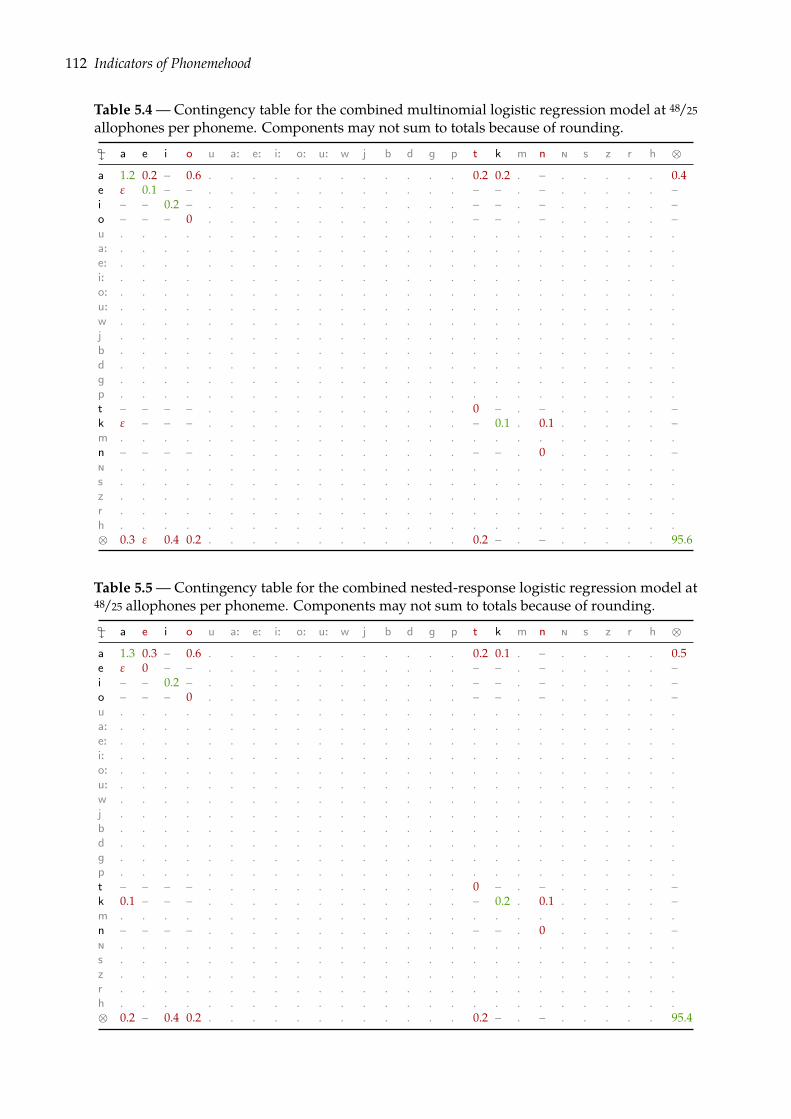
112 Indicators of Phonemehood
Table 5.4 — Contingency table for the combined multinomial logistic regression model at 48/25
allophones per phoneme. Components may not sum to totals because of rounding.
" a e i o u a: e: i: o: u: w j b d g p t k m n ð s z r h ⊗a 1.2 0.2 – 0.6 . . . . . . . . . . . . 0.2 0.2 . – . . . . . 0.4e ε 0.1 – – . . . . . . . . . . . . – – . – . . . . . –i – – 0.2 – . . . . . . . . . . . . – – . – . . . . . –o – – – 0 . . . . . . . . . . . . – – . – . . . . . –u . . . . . . . . . . . . . . . . . . . . . . . . . .a: . . . . . . . . . . . . . . . . . . . . . . . . . .e: . . . . . . . . . . . . . . . . . . . . . . . . . .i: . . . . . . . . . . . . . . . . . . . . . . . . . .o: . . . . . . . . . . . . . . . . . . . . . . . . . .u: . . . . . . . . . . . . . . . . . . . . . . . . . .w . . . . . . . . . . . . . . . . . . . . . . . . . .j . . . . . . . . . . . . . . . . . . . . . . . . . .b . . . . . . . . . . . . . . . . . . . . . . . . . .d . . . . . . . . . . . . . . . . . . . . . . . . . .g . . . . . . . . . . . . . . . . . . . . . . . . . .p . . . . . . . . . . . . . . . . . . . . . . . . . .t – – – – . . . . . . . . . . . . 0 – . – . . . . . –k ε – – – . . . . . . . . . . . . – 0.1 . 0.1 . . . . . –m . . . . . . . . . . . . . . . . . . . . . . . . . .n – – – – . . . . . . . . . . . . – – . 0 . . . . . –ð . . . . . . . . . . . . . . . . . . . . . . . . . .s . . . . . . . . . . . . . . . . . . . . . . . . . .z . . . . . . . . . . . . . . . . . . . . . . . . . .r . . . . . . . . . . . . . . . . . . . . . . . . . .h . . . . . . . . . . . . . . . . . . . . . . . . . .⊗ 0.3 ε 0.4 0.2 . . . . . . . . . . . . 0.2 – . – . . . . . 95.6
Table 5.5—Contingency table for the combined nested-response logistic regression model at48/25 allophones per phoneme. Components may not sum to totals because of rounding.
" a e i o u a: e: i: o: u: w j b d g p t k m n ð s z r h ⊗a 1.3 0.3 – 0.6 . . . . . . . . . . . . 0.2 0.1 . – . . . . . 0.5e ε 0 – – . . . . . . . . . . . . – – . – . . . . . –i – – 0.2 – . . . . . . . . . . . . – – . – . . . . . –o – – – 0 . . . . . . . . . . . . – – . – . . . . . –u . . . . . . . . . . . . . . . . . . . . . . . . . .a: . . . . . . . . . . . . . . . . . . . . . . . . . .e: . . . . . . . . . . . . . . . . . . . . . . . . . .i: . . . . . . . . . . . . . . . . . . . . . . . . . .o: . . . . . . . . . . . . . . . . . . . . . . . . . .u: . . . . . . . . . . . . . . . . . . . . . . . . . .w . . . . . . . . . . . . . . . . . . . . . . . . . .j . . . . . . . . . . . . . . . . . . . . . . . . . .b . . . . . . . . . . . . . . . . . . . . . . . . . .d . . . . . . . . . . . . . . . . . . . . . . . . . .g . . . . . . . . . . . . . . . . . . . . . . . . . .p . . . . . . . . . . . . . . . . . . . . . . . . . .t – – – – . . . . . . . . . . . . 0 – . – . . . . . –k 0.1 – – – . . . . . . . . . . . . – 0.2 . 0.1 . . . . . –m . . . . . . . . . . . . . . . . . . . . . . . . . .n – – – – . . . . . . . . . . . . – – . 0 . . . . . –ð . . . . . . . . . . . . . . . . . . . . . . . . . .s . . . . . . . . . . . . . . . . . . . . . . . . . .z . . . . . . . . . . . . . . . . . . . . . . . . . .r . . . . . . . . . . . . . . . . . . . . . . . . . .h . . . . . . . . . . . . . . . . . . . . . . . . . .⊗ 0.2 – 0.4 0.2 . . . . . . . . . . . . 0.2 – . – . . . . . 95.4
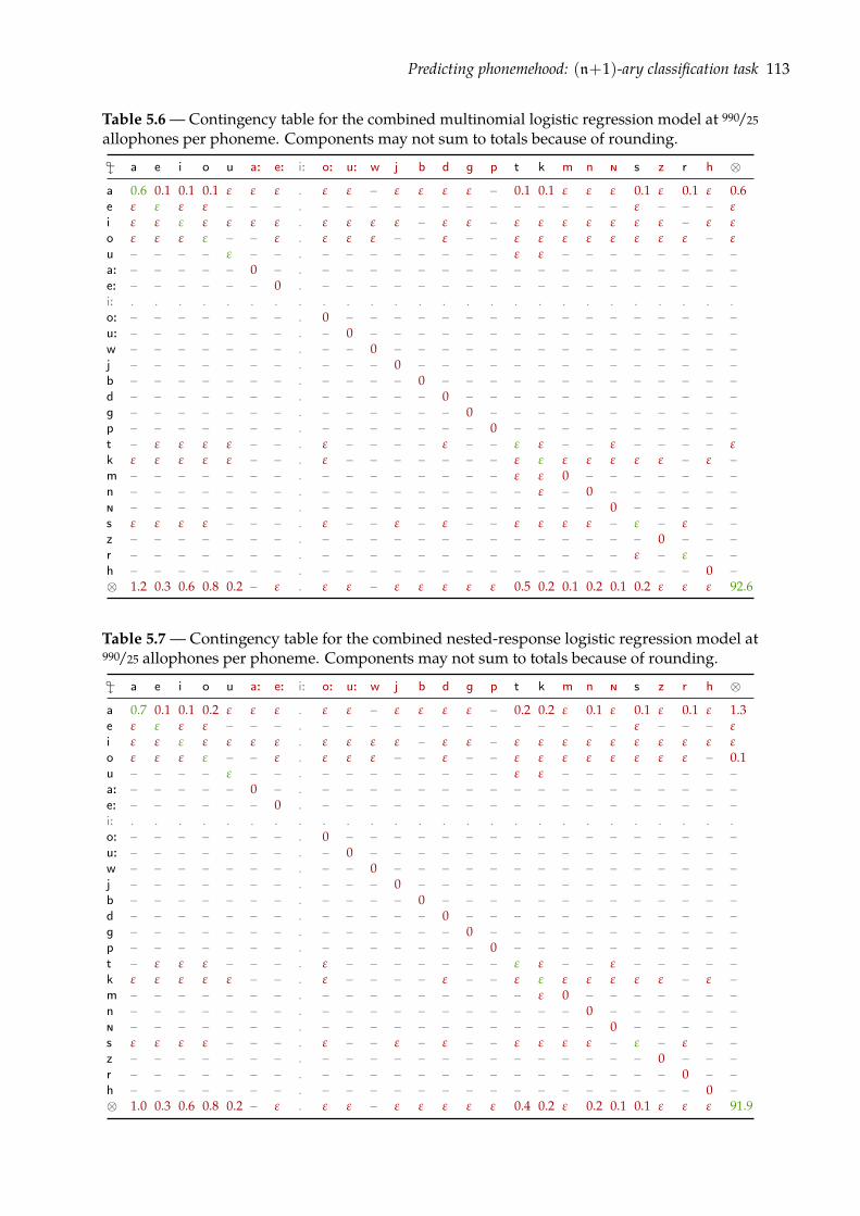
Predicting phonemehood: (n+1)-ary classification task 113
Table 5.6 — Contingency table for the combined multinomial logistic regression model at 990/25
allophones per phoneme. Components may not sum to totals because of rounding.
" a e i o u a: e: i: o: u: w j b d g p t k m n ð s z r h ⊗a 0.6 0.1 0.1 0.1 ε ε ε . ε ε – ε ε ε ε – 0.1 0.1 ε ε ε 0.1 ε 0.1 ε 0.6e ε ε ε ε – – – . – – – – – – – – – – – – – ε – – – εi ε ε ε ε ε ε ε . ε ε ε ε – ε ε – ε ε ε ε ε ε ε – ε εo ε ε ε ε – – ε . ε ε ε – – ε – – ε ε ε ε ε ε ε ε – εu – – – – ε – – . – – – – – – – – ε ε – – – – – – – –a: – – – – – 0 – . – – – – – – – – – – – – – – – – – –e: – – – – – – 0 . – – – – – – – – – – – – – – – – – –i: . . . . . . . . . . . . . . . . . . . . . . . . . .o: – – – – – – – . 0 – – – – – – – – – – – – – – – – –u: – – – – – – – . – 0 – – – – – – – – – – – – – – – –w – – – – – – – . – – 0 – – – – – – – – – – – – – – –j – – – – – – – . – – – 0 – – – – – – – – – – – – – –b – – – – – – – . – – – – 0 – – – – – – – – – – – – –d – – – – – – – . – – – – – 0 – – – – – – – – – – – –g – – – – – – – . – – – – – – 0 – – – – – – – – – – –p – – – – – – – . – – – – – – – 0 – – – – – – – – – –t – ε ε ε ε – – . ε – – – – ε – – ε ε – – ε – – – – εk ε ε ε ε ε – – . ε – – – – – – – ε ε ε ε ε ε ε – ε –m – – – – – – – . – – – – – – – – ε ε 0 – – – – – – –n – – – – – – – . – – – – – – – – – ε – 0 – – – – – –ð – – – – – – – . – – – – – – – – – – – – 0 – – – – –s ε ε ε ε – – – . ε – – ε – ε – – ε ε ε ε – ε – ε – –z – – – – – – – . – – – – – – – – – – – – – – 0 – – –r – – – – – – – . – – – – – – – – – – – – – ε – ε – –h – – – – – – – . – – – – – – – – – – – – – – – – 0 –⊗ 1.2 0.3 0.6 0.8 0.2 – ε . ε ε – ε ε ε ε ε 0.5 0.2 0.1 0.2 0.1 0.2 ε ε ε 92.6
Table 5.7 —Contingency table for the combined nested-response logistic regression model at990/25 allophones per phoneme. Components may not sum to totals because of rounding.
" a e i o u a: e: i: o: u: w j b d g p t k m n ð s z r h ⊗a 0.7 0.1 0.1 0.2 ε ε ε . ε ε – ε ε ε ε – 0.2 0.2 ε 0.1 ε 0.1 ε 0.1 ε 1.3e ε ε ε ε – – – . – – – – – – – – – – – – – ε – – – εi ε ε ε ε ε ε ε . ε ε ε ε – ε ε – ε ε ε ε ε ε ε ε ε εo ε ε ε ε – – ε . ε ε ε – – ε – – ε ε ε ε ε ε ε ε – 0.1u – – – – ε – – . – – – – – – – – ε ε – – – – – – – –a: – – – – – 0 – . – – – – – – – – – – – – – – – – – –e: – – – – – – 0 . – – – – – – – – – – – – – – – – – –i: . . . . . . . . . . . . . . . . . . . . . . . . . .o: – – – – – – – . 0 – – – – – – – – – – – – – – – – –u: – – – – – – – . – 0 – – – – – – – – – – – – – – – –w – – – – – – – . – – 0 – – – – – – – – – – – – – – –j – – – – – – – . – – – 0 – – – – – – – – – – – – – –b – – – – – – – . – – – – 0 – – – – – – – – – – – – –d – – – – – – – . – – – – – 0 – – – – – – – – – – – –g – – – – – – – . – – – – – – 0 – – – – – – – – – – –p – – – – – – – . – – – – – – – 0 – – – – – – – – – –t – ε ε ε – – – . ε – – – – – – – ε ε – – ε – – – – –k ε ε ε ε ε – – . ε – – – – ε – – ε ε ε ε ε ε ε – ε –m – – – – – – – . – – – – – – – – – ε 0 – – – – – – –n – – – – – – – . – – – – – – – – – – – 0 – – – – – –ð – – – – – – – . – – – – – – – – – – – – 0 – – – – –s ε ε ε ε – – – . ε – – ε – ε – – ε ε ε ε – ε – ε – –z – – – – – – – . – – – – – – – – – – – – – – 0 – – –r – – – – – – – . – – – – – – – – – – – – – – – 0 – –h – – – – – – – . – – – – – – – – – – – – – – – – 0 –⊗ 1.0 0.3 0.6 0.8 0.2 – ε . ε ε – ε ε ε ε ε 0.4 0.2 ε 0.2 0.1 0.1 ε ε ε 91.9
114 Indicators of Phonemehood
Finally, strictly positive off-diagonal elements (wrong classifications) are in red, and strictlypositive on-diagonal elements (accurate classifications) are in green.
All four tables corroborate our prior observations that multinomial logistic regression modelsare overwhelmed by non-allophonic pairs, and that the only phonemes whose performancedoes not appear to be due to chance are the most frequent ones. Indeed, even at maximalallophonic complexity, correctly rejected non-allophonic pairs account for approximately 92%of all predictions. Furthermore, the contingency tables for the nested-response model give anadditional example of a frequency effect: the only phonemes as which pairs of phones werewrongfully classified are the aforementioned most frequent phonemes in Japanese, i.e. /a/, /e/,/i/, /o/, /u/, /t/, /k/, and /s/. In order to allow for a better discovery of the phonemic inventory,it thus appears necessary to minimize the impact of non-allophonic pairs.
5.3 Overall assessment
In this chapter, we addressed the limitations of Peperkamp et al.’s (2006) framework for thediscovery of allophony and phonemehood. We showed in Section 5.1 that formal and empiricallimitations arise from its pairwise formulation. On one hand, Peperkamp et al.’s frameworkleaves unspecified the question of the transitivity of allophony. On the other hand, it cannotaccomodate low-variability phonemes or—to say the least—phonemes that received a singleallophone in the quantized representation of the input.
We then carried out various classification experiments whose results unambiguously indicatethat the pairwise formulation strongly impedes the discovery of the phonemic inventory of thetarget language. For instance, we showed in Section 5.2 that, whereas classifying all possiblephone pairs in a given allophonic inventory appears to be quite an easy task, the high performancein predictions we observed is mostly due to the correct ⊗-rejection of non-allophonic pairs.Moreover, as we have argued since Chapter 4, non-allophonic pairs are simply the spuriousbyproduct of a combinatioral enumeration as, in the perspective of the discovery of phonemes,only allophonic pairs are informative.For these reasons, the experiments to be presented in the next chapter consist in a complete
reformulation of Peperkamp et al.’s (2006) framework so that individual phones—rather thanpairs of phones—become the elementary objects to be manipulated. In order to do so, we willcreate a new representation for the input data, and recast the task of acquiring phonemes as astandard partitioning-clustering problem.
CHAPTER 6PHONEMEHOOD REDUX
In this chapter, we propose a complete reformulation of Peperkamp et al.’s (2006) frameworkso that individual phones—rather than pairs of phones—become the elementary objects to bemanipulated. We indeed showed in the preceding chapters of this study that Peperkamp et al.’sframework suffers from the considerable number and smeared distribution of non-allophonicpairs, for all (combinations of) indicators of allophony and at any allophonic complexity. More-over, we have argued that non-allophonic pairs are ultimately irrelevant for the purpose ofdiscovering the phonemic inventory of the target language as they are simply the spuriousbyproduct of a combinatorial enumeration. For these reasons, we shift the primitive data struc-ture from a pair of phones to a single phone. To this aim, we use the phone-to-phone dissimilarityratings provided by (a combination of) indicators of allophony to define points in a Euclideanspace so that each phone in the allophonic inventory is represented by a point in the Euclideanspace, and that the point-to-point distances correspond to the phone-to-phone dissimilarities.Under such a representation, the phonemic inventory of the target language can eventually belearned directly from a partition of a given allophonic inventory whereby each subset in thepartition is to be interpreted as a putative phoneme.
This chapter is divided into six main sections. In Section 6.1, we present the fundamentalprinciples of three-way multidimensional scaling, the statistical technique we used to computea novel, pair-free representation for each indicator of allophony (or combination thereof). InSection 6.2, we present a first assessment of indicators’ phoneme-wise informativeness in terms ofprognoses of phonemehood. Various classification and clustering experiments are then reportedin Sections 6.3, 6.4, and 6.5. Finally, Section 6.6 contains a general assessment of the workpresented in this chapter.
6.1 Shifting the primitive data structure
As we argued in Section 5.1.1, phonemehood is a polyadic relation that exhaustively describesthe realizations of each and every phoneme in the target language, whereas allophony is a binaryrelation that merely indicates whether two phones are realizations of the same phoneme but,in that event, contains no information regarding the identity of the phoneme of which theyboth are realizations. Furthermore, we showed that theoretical and empirical limitations arise(transitivity and hapax phonomena, respectively) when the first step in the discovery of thephonemic inventory of a given language consists in learning the allophony relation between allpossible pairs of phones. These limitations are due to the pairwise nature of Peperkamp et al.’s(2006) framework. For these reasons, our goal in this section is to define a new representation ofthe input data whereby the primitive data structure to be considered by the learner is not a pairof phones, but a single phone.
116 Phonemehood Redux
Unpairing phone pairs In Chapter 4, we showed that the phone-to-phone dissimilarity ratingswe refer to as indicators of allophony are indeed correlated with allophony: non-allophonic pairstend to be more dissimilar than allophonic pairs depending, to a certain extent, on the allophoniccomplexity of the input as well as the linguistic cue each indicator focuses on. As a consequence,we can reasonably consider that indicators of allophony confirm the aforementioned compactnesshypothesis (Duin, 1999; Pękalska et al., 2003) whereby objects that are underlyingly similar (agiven phoneme’s allophones) are also close in their representation (a given indicator’s phone-to-phone dissimilarities). Whereas indicators of allophony have proven to be accurate cuesfor the discovery of phonemes, they however offer no workable representation for the phonesthey rely on. To draw a non-technical analogy, examining an indicator of allophony is akin toobserving a matrix of city-to-city distances as the crow flies, but not having access to a map. Forexample, knowing that Paris is closer to Ruffec than to Los Angeles gives—at a first glance—noinformation on the location of each city. However, the complete matrix of all pairwise distances(e.g. Paris–Ruffec, Paris–Los Angeles, and Ruffec–Los Angeles) can be interpreted as a set ofrelative constraints on the estimation of each city’s location: assuming thatwework in a Euclidean2-dimensional projection of the surface of the Earth (i.e. a commonmap), those three cities definethe vertices of a triangle whose edges’ length are given by the pairwise distances between thecorresponding cities. In this section, we describe the positioning technique we used to infersuch Euclidean embeddings for our allophonic inventories, based on indicators of allophony’sdissimilarity ratings.
6.1.1 Multidimensional scaling
The classic Euclidean embedding technique we used is known as multidimensional scaling (hence-forth MDS; Torgerson, 1952; Groenen & van de Velden, 2004; Borg & Groenen, 2005). Generallyspeaking, the input data used for MDS consist in dissimilarities between pairs of objects, andthe objective of MDS is to represent these dissimilarities as distances between points in a mul-tidimensional Euclidean space such that the distance correspond as closely as possible to thedissimilarities. Following Borg & Groenen (2005), we use MDS as a psychological model that
[explains] perceived dissimilarity as the result of a mental arithmetic that mimic thedistance formula. According to thismodel, themind generates an impression of dissimilarityby adding up the perceived differences of the two objects over their properties.~
In the case at hand, the objective of MDS is to locate n points—i.e. one for each phone—in a low-dimensional Euclidean space in such away that the distances between the points approximate then× n input dissimilarities ∆ of a given indicator of allophony. It is worth noting that previouslydefined phone-to-phone dissimilarity matrices satisfy all the requirements of MDS, as they areby definition square, symmetric, non-negative, and hollow (cf. Section 4.1.2).More precisely, given an a priori dimensionality q ∈N such that 1 ≤ q < n− 1, we want to
find an n× q metric configuration matrix M ≡ [mil ] whereby each phone pi ∈ P in the allophonicinventory is represented by a point mi ≡ (mi1, . . . , miq) in a q-dimensional Euclidean space(if q ≥ n− 1, the solution is trivial; Borg & Groenen, 2005). Furthermore, we want the inputphone-to-phone dissimilarities to constrain the output point-to-point distances. Concretely, letdij(M) denote the Euclidean distance between the points mi and mj, given by
dij(M) ≡√
∑l(mil −mjl)2 where l ∈ (1, 2, . . . , q), (6.1)
we aim at finding the optimal Euclidean embedding of ∆, i.e. the embedding where the outputdistances dij(M) correspond as closely as possible to the input dissimilarities δij.
Stress and SMACOF Following de Leeuw & Mair (2009), we make the optimization problemmore precise by defining the objective stress function σ(M). The stress of a given metric configu-ration M with regards to the input pairwise dissimilarities ∆ and the pairwise weights W is givenby the weighted sum of the squared differences between the corresponding input dissimilarities
Shifting the primitive data structure 117
and output distances (a.k.a. the standard residual sum of squares; Pękalska & Duin, 2005; p. 136).Formally, we have
σ(M; ∆, W) ≡∑i<j
wij(δij − dij(M)
)2. (6.2)
It is worth mentioning that, in the case at hand, the previously defined n× n weight matrices Walso satisfy the assumptions of symmetry, non-negativity, and hollowness (cf. Section 4.3.3).
Because stress values are given by the added differences between corresponding input dissim-ilarities and output distances, this objective function is to be minimized. The iterative strategywe used to minimize the stress function is referred to in the MDS literature as SMACOF (shortfor scaling by majorizing a complicated function; de Leeuw & Mair, 2009). Although describingthe practical details behind this optimization strategy is beyond the scope of this research, it isworth highlighting the fact that SMACOF has the desirable property to guarantee a series ofnon-increasing stress values with a linear convergence rate (de Leeuw, 1988). Put another way,performing an additional iteration of the SMACOF algorithm can not decrease the quality of theoutput configuration. However, depending on the number n of objects in the dataset and thecomposition of the dissimilarity matrix, a large number of iterations may be required if a highaccuracy is needed (Groenen & Heiser, 2000; Bronstein et al., 2005; Rosman et al., 2008).It is worth noting that the optimality of the output metric configuration M only depends
on the input dissimilarities ∆ and the pairwise weights W—no reference data structure suchas P or A∗ is involved in the computation of the stress function. Though it is not a machinelearning technique stricto sensu, MDS is thus to be considered unsupervised or—to say theleast—unaware of the true structure of the data it manipulates.
Strike a pose, there’s nothing to it! Because Euclidean distances are preserved under rotation,translation, and reflection, these operations may be applied to a given metric configurationwithout affecting its stress. Extending our prior analogy with geographic distances, the distancebetween Paris and Los Angeles is not affected by turning the map upside down or, simply,the rotation of the Earth. Most MDS programs rely on this insensitivity to distance-preservingtransformations (i.e. isometries) and, for the sake of efficiency, computemetric configurations thatare only determined up to location (Venables & Ripley, 2002; R Development Core Team, 2010;cf. stats::cmdscale and mass::isoMDS). In other words, distinct metric configurations may haveequal (and optimal) stress valueswith regards to a given input dissimilaritymatrix. Consequently,it is worth noting that althoughMDS outputs workable location estimates, individual coordinatesand dimensions are not meaningful.
Non-metric SMACOF In Chapter 4, we only constrained indicators of allophony to be symmet-ric, non-negative dissimilarity measures. Therefore, we did not constrain indicators to be truemetrics as neither the identity of indiscernibles (i.e. ∀ pi, pj ⊆ P, δij = 0 ⇒ pi = pj) nor thetriangle inequality (i.e. ∀ pi, pi′ , pj ⊆ P, δij ≤ δii′ + δi′ j) were enforced. In the perspective of aEuclidean—hence metric—embedding, such dissimilarities are considered to convey qualitativeinstead of quantitative information (Pękalska & Duin, 2005): whereas dissimilarities conveymore information than a mere pairwise ranking (cf. Section 5.2), they can not be used as theyare to infer sound location estimates. We can consequently think of transformations of thedissimilarities that—while preserving the pairwise ranking, to the bare minimum—allow fora better fit of the configuration M in the Euclidean space. If such a transformation f obeysthe monotonicity constraint that δij < δi′ j′ ⇒ f (δij) < f (δi′ j′), the MDS procedure is referredto as non-metric (Shepard, 1962a,b; Borg & Groenen, 2005; de Leeuw & Mair, 2009) and thecorresponding non-metric stress function becomes
σ(M, f ; ∆, W) ≡∑i<j
wij(
f (δij)− dij(M))2. (6.3)
In non-metric MDS, the monotonic transformation f is determined and optimized by the pro-gram together with the metric configuration M. In our experiments, the optimal monotonic
118 Phonemehood Redux
transformation f was recomputed after each SMACOF iteration (setting the parameter modulusto 1 in smacof; de Leeuw &Mair, 2009).
Transforming the observed dissimilarity matrix ∆ calls for a proper treatment of tied values, i.e.when δij = δi′ j′ for two phone pairs pi, pj and pi′ , pj′. In that case, two different approachesare commonly suggested in the MDS literature: the unrestrictive (a.k.a. primary) approach thatdoes not necessarily requires that transforming ties yields ties, i.e. δij = δi′ j′ ; f (δij) = f (δi′ j′),and the restrictive (a.k.a. secondary) approach that does (de Leeuw &Mair, 2009). In the absenceof a priori linguistic knowledge that would justify the use of the restrictive approach—we can notinterpret ties in a given indicator’s values, except as numerical accidents—we chose to consideronly the unrestrictive approach in our experiments.
Three-way SMACOF In its classic definition, MDS can only accomodate one input dissimilaritymatrix ∆, and this approach to Euclidean embedding is known as two-way (i.e. phone to phone)MDS. Various extensions of the original MDS procedure have been proposed to infer a singlemetric configuration from various dissimilarity matrices. In the case at hand, such extensionsallow us to combine κ different indicators of allophony ∆1, . . . , ∆κ (typically an acoustic, atemporal, a distributional, and a lexical indicator) into a single metric configuration.Combining κ separate n× n dissimilarity matrices into a single n× q group configuration
Z, to be defined hereafter, is known as MDS for individual differences and three-way MDS (i.e.phone to phone to indicator; Horan, 1969; Borg & Groenen, 2005; de Leeuw & Mair, 2009). Thetypical setting for three-way MDS arises when n× n dissimilarity ratings are available from κdifferent—yet comparable—data sources, e.g. subjects, replications, or indicators of allophony.The objective of three-way MDS is best summarized in the title of Horan’s (1969) seminal study:
Combining observations when individuals have different perceptual structures.~Indeed, the major assumption behind three-way MDS is that individual spaces are systematicaldistortions of a shared space (MDS(X) User Manual, 1981). Thus, even though the optimizationinvolves the computation of a configuration matrix Mk for each individual, the standard strategyconsists in introducing restrictions on the configurations Mk in terms of a linear decomposition
Mk ≡ ZRk, (6.4)where Z ≡ [zil ] is the n × q shared group configuration and each Rk ≡ [rll′k] is an individualq× q regression weight matrix to be estimated simultaneously (de Leeuw & Mair, 2009). Asemphasized in the MDS(X) User Manual (1981), the group configuration Z is a compromisebetween all individuals’ configurations, and it may conceivably describe the configuration of nosingle individual.
In the case of three-way MDS, the stress of the group configuration is given by the sum of thestress values of the individual configurations. Formally, we have
σ(Z, R1, f1, . . . , Rκ, fκ; ∆1, . . . , ∆κ, W) ≡ ∑k
σ(ZRk, fk; ∆k, W) (6.5)
= ∑i<j
wij
(∑
k
(fk(δijk)− dij(ZRk)
)2)
(6.6)
It is worth noting that this definition is somewhat simpler than the one given by de Leeuw &Mair (2009; eq. 21, p. 7). This simplification arises from the fact that, in the case at hand, weightsare not conditional on the individuals (i.e. all indicators share the same weighting scheme) and,hence, we rely on a single weight matrix W rather than κ different weight matrices.All in all, given weighted three-way dissimilarities data, the objective of a three-way MDS
procedure is to solve simultaneously for the group configuration Z, the individual regressionmatrices R1, . . . , Rκ, and the monotonic transformations f1, . . . , fκ, so as to optimize the fit of thegroup configuration to the (monotonically transformed) dissimilarities data.
Individual differences In order to control to which extent each individual space is a distortionof the underlying group space, we introduce further restrictions in the definition of three-way
Shifting the primitive data structure 119
MDS. To do so, we constrain the form of the individual regression matrices R1, . . . , Rκ (Horan,1969; Carroll & Chang, 1970; MDS(X) User Manual, 1981; de Leeuw & Mair, 2009). We considerthree standard variations of the abovementioned model, ranging from fully unconstrained tofully constrained.If no constraint is imposed, i.e. every regression matrix Rk is a general matrix, the model
is known as the generalized Euclidean model (a.k.a. IDIOSCAL, short for individual differences inorientation scaling) as it relies on the generalized Euclidean distance
dij(Mk) ≡ dij(ZRk) ≡√
∑l
∑l′
ull′k(zil − zjl)(zil′ − zjl′), (6.7)
where Uk ≡ RkRTk . Under this unconstrained model, every individual systematically transforms
the group space first by a rotation or a reflection, and then by scaling each dimension.If every regression matrix Rk is constrained to be a diagonal matrix, then Uk ≡ RkRT
k = R2k is
also diagonal. The corresponding MDS model is known as the weighted Euclidean model (a.k.a.INDSCAL, short for individual differences scaling), and the underlyingweighted Euclidean distancecan straightforwardly be defined as
dij(Mk) ≡ dij(ZRk) ≡√
∑l
r2llk(zil − zjl)2. (6.8)
Under this model, scaling becomes the only possible individual transformation. In other words,thismodel explains differences between individuals by a differential weighting of each dimensionby each individual (MDS(X) User Manual, 1981), i.e. all indicators rely on the same underlyinggroup space, but different dimensions of that space may be more or less salient to each indicator.Finally, if every regression matrix Rk is further constrained to be an identity matrix, we have
Mk ≡ ZRk = Z. This model, the simplest of all three-way MDS models we consider in this study,is known as the unweighted Euclidean model (a.k.a. the identity model), and the definition of thedistance function can be simplified to the usual Euclidean distance, i.e.
dij(Mk) ≡ dij(Z) ≡√
∑l(zil − zjl)2 (6.9)
Under this very constrained model, no individual transformation is allowed and, hence, individ-ual spaces do not depart from the group space.
In Chapter 4, we computed various (acoustic, temporal, distributional, and lexical) indicatorsto assess the allophonic dissimilarity of all pairs of phones in a given allophonic inventory. Weare however unable not assert that indicators of different classes use the response scale andthe underlying (phonological) group space in identical ways. In fact, in light of the recurrentdiscrepancies in performance we observed in Chapters 4 and 5 between all four indicator classes,we are able to assert that they do not use the group space identically. Our dissimilarity mea-surements are thus conditional on each indicator: all observations within a dissimilarity matrixare comparable, but not corresponding observations between matrices (a property commonlyreferred to as matrix-conditionality or split-by-matrices in the three-way MDS literature; Borg &Groenen, 2005). Whereas, for instance, it would be meaningful to say that a given phone pairis acoustically twice as dissimilar as another phone pair, it would make no sense to say that agiven phone pair is acoustically twice as dissimilar as it is distributionally.For this reason, the unweighted Euclidean model—whereby no individual transformation is
possible—appears to be too restrictive for the case at hand, especially compared to the generalizedEuclidean (IDIOSCAL) and the weighted Euclidean (INDSCAL) models. The difference betweenthese two models arises from the fact that scaling, rotations, and reflections are permissible inthe former, while only scaling is permissible in the latter. As in the case of tied values, we favoredan unrestricted approach in our experiments: in the absence of a priori linguistic knowledge thatwould oppose the use of rotations and reflections in the computation of the optimal Euclideanembedding of an allophonic inventory from three-way dissimilarity data, all MDS configurationsto be further examined were computed under the generalized Euclidean model.
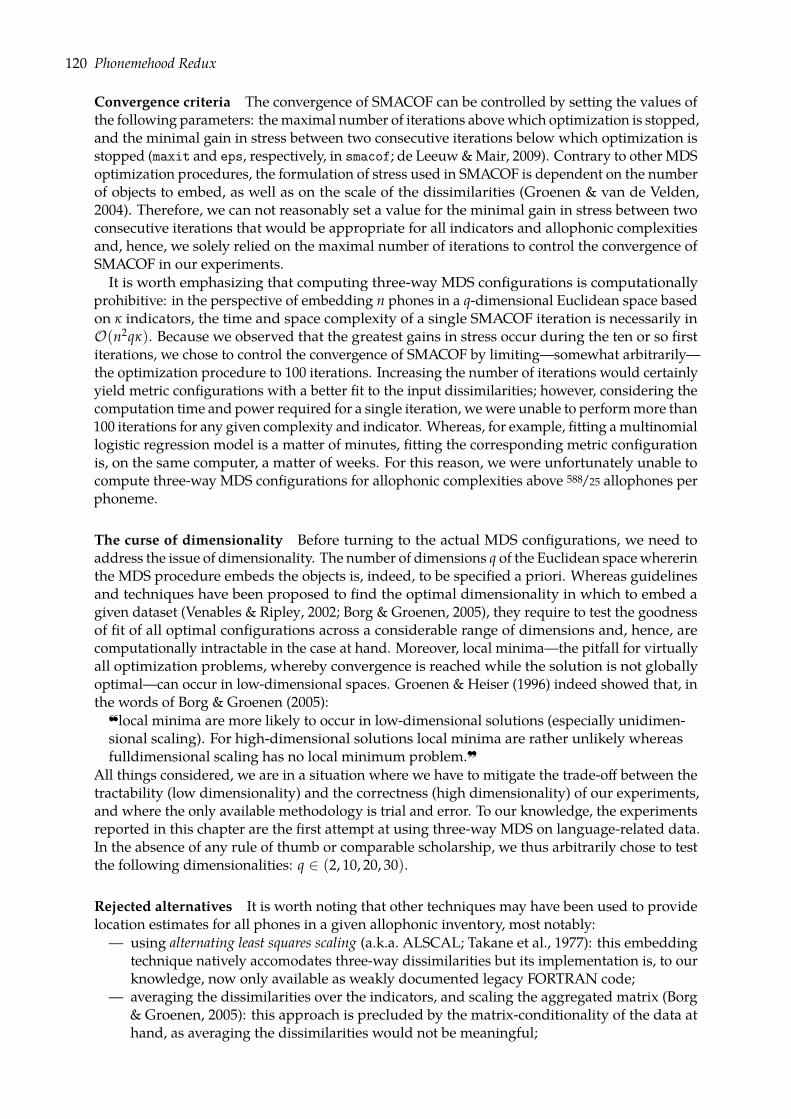
120 Phonemehood Redux
Convergence criteria The convergence of SMACOF can be controlled by setting the values ofthe following parameters: themaximal number of iterations abovewhich optimization is stopped,and the minimal gain in stress between two consecutive iterations below which optimization isstopped (maxit and eps, respectively, in smacof; de Leeuw&Mair, 2009). Contrary to other MDSoptimization procedures, the formulation of stress used in SMACOF is dependent on the numberof objects to embed, as well as on the scale of the dissimilarities (Groenen & van de Velden,2004). Therefore, we can not reasonably set a value for the minimal gain in stress between twoconsecutive iterations that would be appropriate for all indicators and allophonic complexitiesand, hence, we solely relied on the maximal number of iterations to control the convergence ofSMACOF in our experiments.It is worth emphasizing that computing three-way MDS configurations is computationally
prohibitive: in the perspective of embedding n phones in a q-dimensional Euclidean space basedon κ indicators, the time and space complexity of a single SMACOF iteration is necessarily inO(n2qκ). Because we observed that the greatest gains in stress occur during the ten or so firstiterations, we chose to control the convergence of SMACOF by limiting—somewhat arbitrarily—the optimization procedure to 100 iterations. Increasing the number of iterations would certainlyyield metric configurations with a better fit to the input dissimilarities; however, considering thecomputation time and power required for a single iteration, wewere unable to performmore than100 iterations for any given complexity and indicator. Whereas, for example, fitting amultinomiallogistic regression model is a matter of minutes, fitting the corresponding metric configurationis, on the same computer, a matter of weeks. For this reason, we were unfortunately unable tocompute three-way MDS configurations for allophonic complexities above 588/25 allophones perphoneme.
The curse of dimensionality Before turning to the actual MDS configurations, we need toaddress the issue of dimensionality. The number of dimensions q of the Euclidean spacewhererinthe MDS procedure embeds the objects is, indeed, to be specified a priori. Whereas guidelinesand techniques have been proposed to find the optimal dimensionality in which to embed agiven dataset (Venables & Ripley, 2002; Borg & Groenen, 2005), they require to test the goodnessof fit of all optimal configurations across a considerable range of dimensions and, hence, arecomputationally intractable in the case at hand. Moreover, local minima—the pitfall for virtuallyall optimization problems, whereby convergence is reached while the solution is not globallyoptimal—can occur in low-dimensional spaces. Groenen & Heiser (1996) indeed showed that, inthe words of Borg & Groenen (2005):
local minima are more likely to occur in low-dimensional solutions (especially unidimen-sional scaling). For high-dimensional solutions local minima are rather unlikely whereasfulldimensional scaling has no local minimum problem.~
All things considered, we are in a situation where we have to mitigate the trade-off between thetractability (low dimensionality) and the correctness (high dimensionality) of our experiments,and where the only available methodology is trial and error. To our knowledge, the experimentsreported in this chapter are the first attempt at using three-way MDS on language-related data.In the absence of any rule of thumb or comparable scholarship, we thus arbitrarily chose to testthe following dimensionalities: q ∈ (2, 10, 20, 30).
Rejected alternatives It is worth noting that other techniques may have been used to providelocation estimates for all phones in a given allophonic inventory, most notably:— using alternating least squares scaling (a.k.a. ALSCAL; Takane et al., 1977): this embedding
technique natively accomodates three-way dissimilarities but its implementation is, to ourknowledge, now only available as weakly documented legacy FORTRAN code;
— averaging the dissimilarities over the indicators, and scaling the aggregated matrix (Borg& Groenen, 2005): this approach is precluded by the matrix-conditionality of the data athand, as averaging the dissimilarities would not be meaningful;
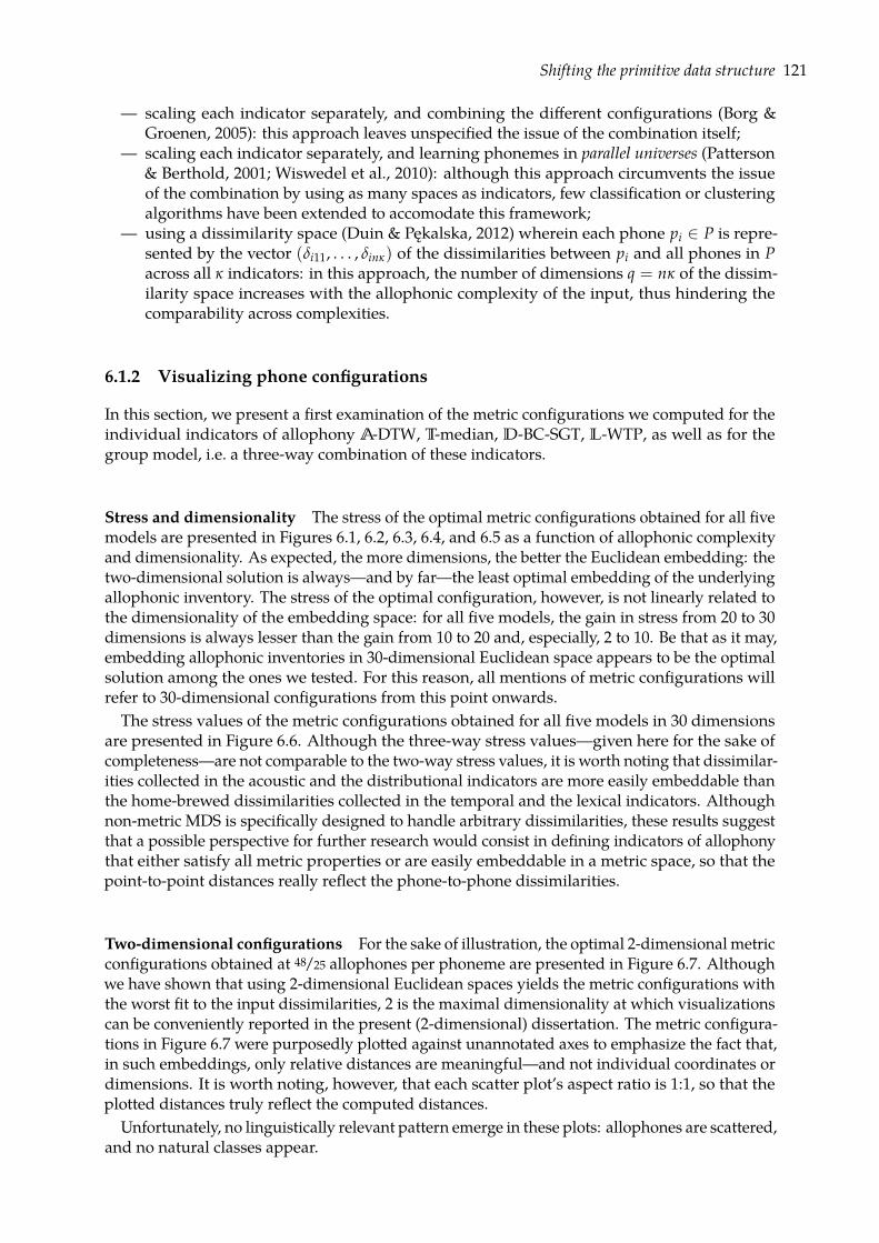
Shifting the primitive data structure 121
— scaling each indicator separately, and combining the different configurations (Borg &Groenen, 2005): this approach leaves unspecified the issue of the combination itself;
— scaling each indicator separately, and learning phonemes in parallel universes (Patterson& Berthold, 2001; Wiswedel et al., 2010): although this approach circumvents the issueof the combination by using as many spaces as indicators, few classification or clusteringalgorithms have been extended to accomodate this framework;
— using a dissimilarity space (Duin & Pękalska, 2012) wherein each phone pi ∈ P is repre-sented by the vector (δi11, . . . , δinκ) of the dissimilarities between pi and all phones in Pacross all κ indicators: in this approach, the number of dimensions q = nκ of the dissim-ilarity space increases with the allophonic complexity of the input, thus hindering thecomparability across complexities.
6.1.2 Visualizing phone configurations
In this section, we present a first examination of the metric configurations we computed for theindividual indicators of allophony A-DTW, T-median, D-BC-SGT, L-WTP, as well as for thegroup model, i.e. a three-way combination of these indicators.
Stress and dimensionality The stress of the optimal metric configurations obtained for all fivemodels are presented in Figures 6.1, 6.2, 6.3, 6.4, and 6.5 as a function of allophonic complexityand dimensionality. As expected, the more dimensions, the better the Euclidean embedding: thetwo-dimensional solution is always—and by far—the least optimal embedding of the underlyingallophonic inventory. The stress of the optimal configuration, however, is not linearly related tothe dimensionality of the embedding space: for all five models, the gain in stress from 20 to 30dimensions is always lesser than the gain from 10 to 20 and, especially, 2 to 10. Be that as it may,embedding allophonic inventories in 30-dimensional Euclidean space appears to be the optimalsolution among the ones we tested. For this reason, all mentions of metric configurations willrefer to 30-dimensional configurations from this point onwards.The stress values of the metric configurations obtained for all five models in 30 dimensions
are presented in Figure 6.6. Although the three-way stress values—given here for the sake ofcompleteness—are not comparable to the two-way stress values, it is worth noting that dissimilar-ities collected in the acoustic and the distributional indicators are more easily embeddable thanthe home-brewed dissimilarities collected in the temporal and the lexical indicators. Althoughnon-metric MDS is specifically designed to handle arbitrary dissimilarities, these results suggestthat a possible perspective for further research would consist in defining indicators of allophonythat either satisfy all metric properties or are easily embeddable in a metric space, so that thepoint-to-point distances really reflect the phone-to-phone dissimilarities.
Two-dimensional configurations For the sake of illustration, the optimal 2-dimensional metricconfigurations obtained at 48/25 allophones per phoneme are presented in Figure 6.7. Althoughwe have shown that using 2-dimensional Euclidean spaces yields the metric configurations withthe worst fit to the input dissimilarities, 2 is the maximal dimensionality at which visualizationscan be conveniently reported in the present (2-dimensional) dissertation. The metric configura-tions in Figure 6.7 were purposedly plotted against unannotated axes to emphasize the fact that,in such embeddings, only relative distances are meaningful—and not individual coordinates ordimensions. It is worth noting, however, that each scatter plot’s aspect ratio is 1:1, so that theplotted distances truly reflect the computed distances.
Unfortunately, no linguistically relevant pattern emerge in these plots: allophones are scattered,and no natural classes appear.
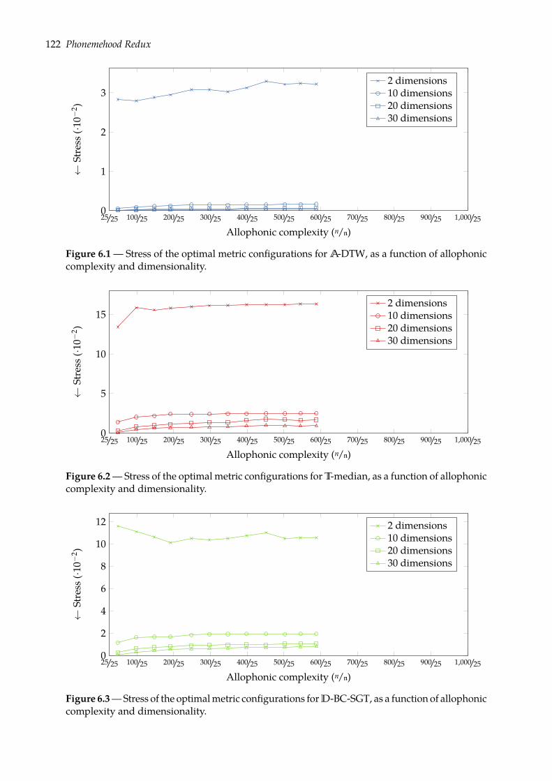
122 Phonemehood Redux
100/25 200/25 300/25 400/25 500/25 600/25 700/25 800/25 900/25 1,000/250
1
2
3
25/25
Allophonic complexity (n/n)
←St
ress
(·10−
2 )2 dimensions10 dimensions20 dimensions30 dimensions
Figure 6.1 — Stress of the optimal metric configurations for A-DTW, as a function of allophoniccomplexity and dimensionality.
100/25 200/25 300/25 400/25 500/25 600/25 700/25 800/25 900/25 1,000/250
5
10
15
25/25
Allophonic complexity (n/n)
←St
ress
(·10−
2 )
2 dimensions10 dimensions20 dimensions30 dimensions
Figure 6.2—Stress of the optimal metric configurations for T-median, as a function of allophoniccomplexity and dimensionality.
100/25 200/25 300/25 400/25 500/25 600/25 700/25 800/25 900/25 1,000/250
2
4
6
8
10
12
25/25
Allophonic complexity (n/n)
←St
ress
(·10−
2 )
2 dimensions10 dimensions20 dimensions30 dimensions
Figure 6.3—Stress of the optimalmetric configurations forD-BC-SGT, as a function of allophoniccomplexity and dimensionality.
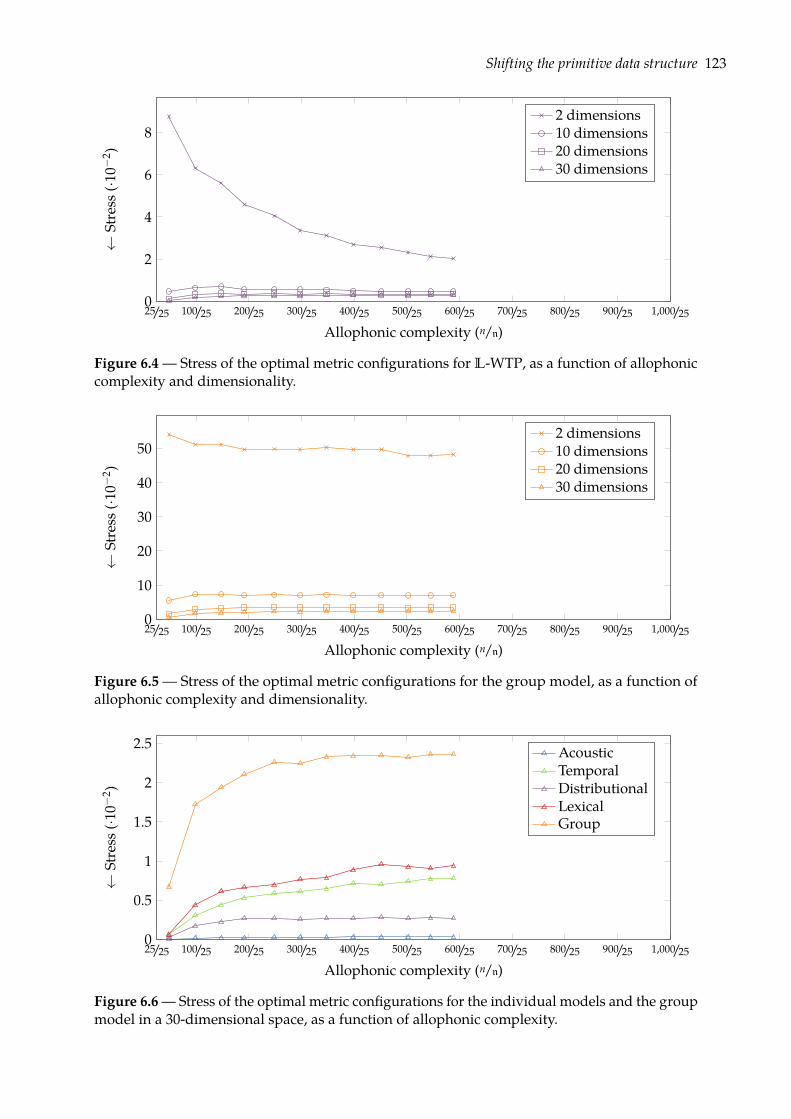
Shifting the primitive data structure 123
100/25 200/25 300/25 400/25 500/25 600/25 700/25 800/25 900/25 1,000/250
2
4
6
8
25/25
Allophonic complexity (n/n)
←St
ress
(·10−
2 )2 dimensions10 dimensions20 dimensions30 dimensions
Figure 6.4 — Stress of the optimal metric configurations for L-WTP, as a function of allophoniccomplexity and dimensionality.
100/25 200/25 300/25 400/25 500/25 600/25 700/25 800/25 900/25 1,000/250
10
20
30
40
50
25/25
Allophonic complexity (n/n)
←St
ress
(·10−
2 )
2 dimensions10 dimensions20 dimensions30 dimensions
Figure 6.5— Stress of the optimal metric configurations for the group model, as a function ofallophonic complexity and dimensionality.
100/25 200/25 300/25 400/25 500/25 600/25 700/25 800/25 900/25 1,000/250
0.5
1
1.5
2
2.5
25/25
Allophonic complexity (n/n)
←St
ress
(·10−
2 )
AcousticTemporalDistributionalLexicalGroup
Figure 6.6—Stress of the optimal metric configurations for the individual models and the groupmodel in a 30-dimensional space, as a function of allophonic complexity.
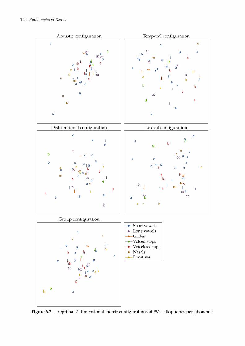
124 Phonemehood Redux
Acoustic configuration Temporal configuration
a
a
a
aa
a
a
a
a
a
e
e
ee
i
i
ii
o
o
o
o
u
a:e:
i:o:
u:w
j
bd
g
pt
t
t
k
kk
m
n
n
ð
sz
r
ha
aaa
a a
a
a
a
a
e
ee
e
i
i
i
i
o
o
o
o
u
a:
e:
i:
o:
u:
w
j
b
d
g
p
t
t
t
k
k
k
m
nn
ð
s
z rh
Distributional configuration Lexical configuration
a
a
a
a
a
a
a a
a a
e
e
e
e
i
i
i
i
o
o
o
ou
a:e:
i:
o:
u:
w
j
b
d
g
p
tt
t
k
k
km
n
n
ð
s
z r h
a
a
a
a
a
aa
a
a
ae
e
e
e
i i ii
o
o
oo
u
a: e:
i:
o:
u:
w
j
b
dg
p
t
t
t
k
kk
m
nn
ð
s
z
r h
Group configuration
a
a
a
a
a
a
a
a
a
ae
e
e
ei
i
ii
o
o
oo
u
a:e:
i:
o:
u:
w
j
b
d
g
p
t
tt
kk
k
m
n
n
ð
szr
h
Short vowelsLong vowelsGlidesVoiced stopsVoiceless stopsNasalsFricatives
Figure 6.7 —Optimal 2-dimensional metric configurations at 48/25 allophones per phoneme.
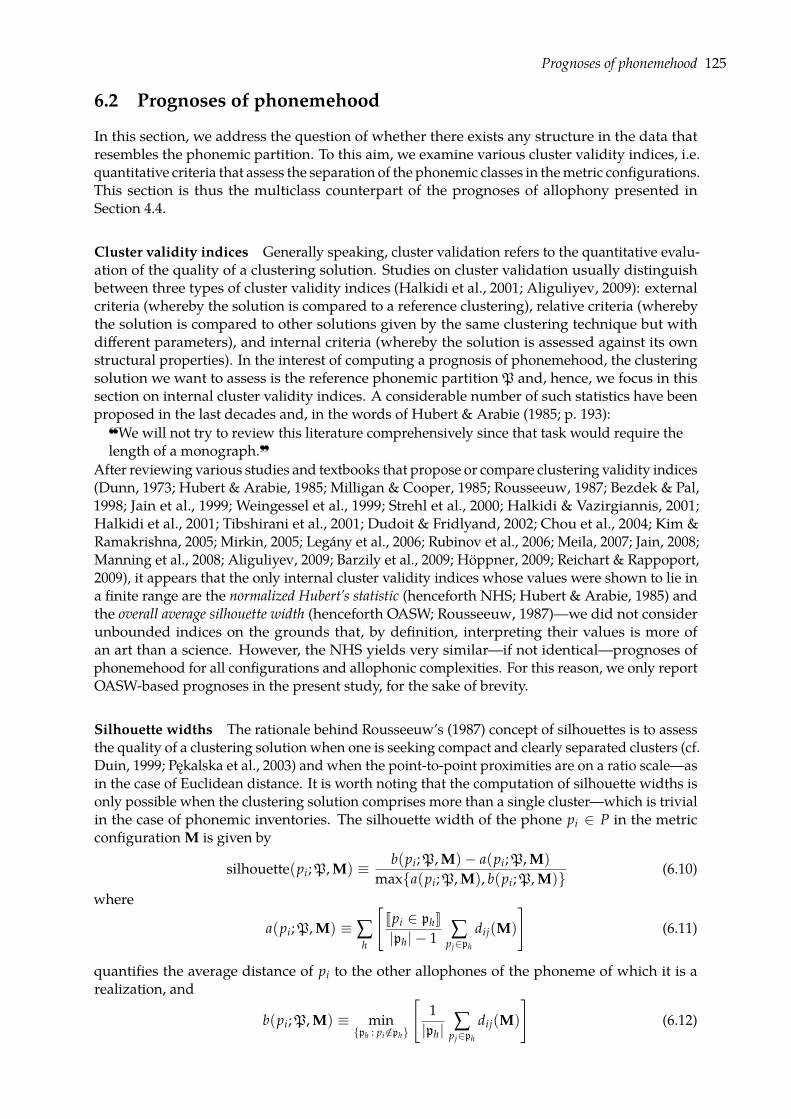
Prognoses of phonemehood 125
6.2 Prognoses of phonemehood
In this section, we address the question of whether there exists any structure in the data thatresembles the phonemic partition. To this aim, we examine various cluster validity indices, i.e.quantitative criteria that assess the separation of the phonemic classes in themetric configurations.This section is thus the multiclass counterpart of the prognoses of allophony presented inSection 4.4.
Cluster validity indices Generally speaking, cluster validation refers to the quantitative evalu-ation of the quality of a clustering solution. Studies on cluster validation usually distinguishbetween three types of cluster validity indices (Halkidi et al., 2001; Aliguliyev, 2009): externalcriteria (whereby the solution is compared to a reference clustering), relative criteria (wherebythe solution is compared to other solutions given by the same clustering technique but withdifferent parameters), and internal criteria (whereby the solution is assessed against its ownstructural properties). In the interest of computing a prognosis of phonemehood, the clusteringsolution we want to assess is the reference phonemic partition P and, hence, we focus in thissection on internal cluster validity indices. A considerable number of such statistics have beenproposed in the last decades and, in the words of Hubert & Arabie (1985; p. 193):
We will not try to review this literature comprehensively since that task would require thelength of a monograph.~
After reviewing various studies and textbooks that propose or compare clustering validity indices(Dunn, 1973; Hubert & Arabie, 1985; Milligan & Cooper, 1985; Rousseeuw, 1987; Bezdek & Pal,1998; Jain et al., 1999; Weingessel et al., 1999; Strehl et al., 2000; Halkidi & Vazirgiannis, 2001;Halkidi et al., 2001; Tibshirani et al., 2001; Dudoit & Fridlyand, 2002; Chou et al., 2004; Kim &Ramakrishna, 2005; Mirkin, 2005; Legány et al., 2006; Rubinov et al., 2006; Meila, 2007; Jain, 2008;Manning et al., 2008; Aliguliyev, 2009; Barzily et al., 2009; Höppner, 2009; Reichart & Rappoport,2009), it appears that the only internal cluster validity indices whose values were shown to lie ina finite range are the normalized Hubert’s statistic (henceforth NHS; Hubert & Arabie, 1985) andthe overall average silhouette width (henceforth OASW; Rousseeuw, 1987)—we did not considerunbounded indices on the grounds that, by definition, interpreting their values is more ofan art than a science. However, the NHS yields very similar—if not identical—prognoses ofphonemehood for all configurations and allophonic complexities. For this reason, we only reportOASW-based prognoses in the present study, for the sake of brevity.
Silhouette widths The rationale behind Rousseeuw’s (1987) concept of silhouettes is to assessthe quality of a clustering solution when one is seeking compact and clearly separated clusters (cf.Duin, 1999; Pękalska et al., 2003) and when the point-to-point proximities are on a ratio scale—asin the case of Euclidean distance. It is worth noting that the computation of silhouette widths isonly possible when the clustering solution comprises more than a single cluster—which is trivialin the case of phonemic inventories. The silhouette width of the phone pi ∈ P in the metricconfiguration M is given by
silhouette(pi;P, M) ≡ b(pi;P, M)− a(pi;P, M)
maxa(pi;P, M), b(pi;P, M) (6.10)
where
a(pi;P, M) ≡∑h
[Jpi ∈ phK|ph| − 1 ∑
pj∈ph
dij(M)
](6.11)
quantifies the average distance of pi to the other allophones of the phoneme of which it is arealization, and
b(pi;P, M) ≡ minph : pi /∈ph
[1|ph| ∑
pj∈ph
dij(M)
](6.12)
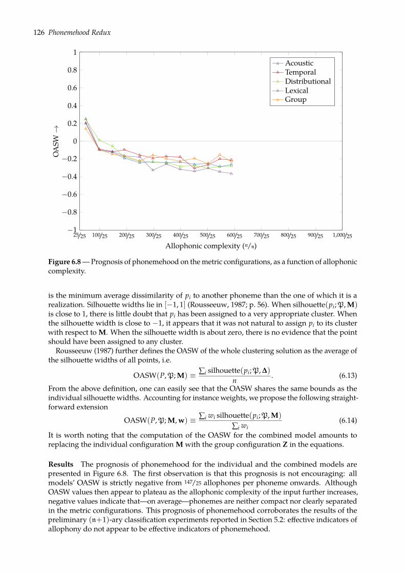
126 Phonemehood Redux
100/25 200/25 300/25 400/25 500/25 600/25 700/25 800/25 900/25 1,000/25−1
−0.8
−0.6
−0.4
−0.2
0
0.2
0.4
0.6
0.8
1
25/25
Allophonic complexity (n/n)
OA
SW→
AcousticTemporalDistributionalLexicalGroup
Figure 6.8—Prognosis of phonemehood on themetric configurations, as a function of allophoniccomplexity.
is the minimum average dissimilarity of pi to another phoneme than the one of which it is arealization. Silhouette widths lie in [−1, 1] (Rousseeuw, 1987; p. 56). When silhouette(pi;P, M)is close to 1, there is little doubt that pi has been assigned to a very appropriate cluster. Whenthe silhouette width is close to −1, it appears that it was not natural to assign pi to its clusterwith respect to M. When the silhouette width is about zero, there is no evidence that the pointshould have been assigned to any cluster.
Rousseeuw (1987) further defines the OASW of the whole clustering solution as the average ofthe silhouette widths of all points, i.e.
OASW(P,P; M) ≡ ∑i silhouette(pi;P, ∆)
n. (6.13)
From the above definition, one can easily see that the OASW shares the same bounds as theindividual silhouette widths. Accounting for instance weights, we propose the following straight-forward extension
OASW(P,P; M, w) ≡ ∑i wi silhouette(pi;P, M)
∑i wi(6.14)
It is worth noting that the computation of the OASW for the combined model amounts toreplacing the individual configuration M with the group configuration Z in the equations.
Results The prognosis of phonemehood for the individual and the combined models arepresented in Figure 6.8. The first observation is that this prognosis is not encouraging: allmodels’ OASW is strictly negative from 147/25 allophones per phoneme onwards. AlthoughOASW values then appear to plateau as the allophonic complexity of the input further increases,negative values indicate that—on average—phonemes are neither compact nor clearly separatedin the metric configurations. This prognosis of phonemehood corroborates the results of thepreliminary (n+1)-ary classification experiments reported in Section 5.2: effective indicators ofallophony do not appear to be effective indicators of phonemehood.
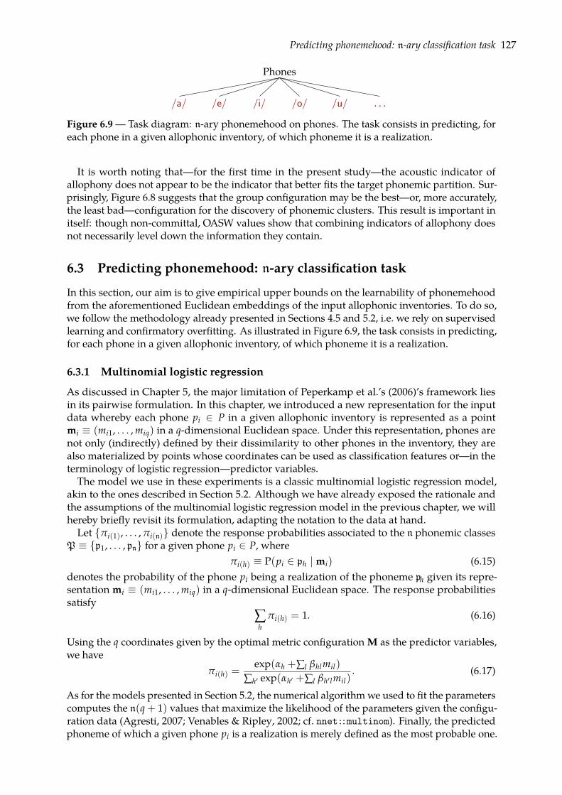
Predicting phonemehood: n-ary classification task 127
Phones
/a/ /e/ /i/ /o/ /u/ . . .
Figure 6.9 — Task diagram: n-ary phonemehood on phones. The task consists in predicting, foreach phone in a given allophonic inventory, of which phoneme it is a realization.
It is worth noting that—for the first time in the present study—the acoustic indicator ofallophony does not appear to be the indicator that better fits the target phonemic partition. Sur-prisingly, Figure 6.8 suggests that the group configuration may be the best—or, more accurately,the least bad—configuration for the discovery of phonemic clusters. This result is important initself: though non-committal, OASW values show that combining indicators of allophony doesnot necessarily level down the information they contain.
6.3 Predicting phonemehood: n-ary classification task
In this section, our aim is to give empirical upper bounds on the learnability of phonemehoodfrom the aforementioned Euclidean embeddings of the input allophonic inventories. To do so,we follow the methodology already presented in Sections 4.5 and 5.2, i.e. we rely on supervisedlearning and confirmatory overfitting. As illustrated in Figure 6.9, the task consists in predicting,for each phone in a given allophonic inventory, of which phoneme it is a realization.
6.3.1 Multinomial logistic regression
As discussed in Chapter 5, the major limitation of Peperkamp et al.’s (2006)’s framework liesin its pairwise formulation. In this chapter, we introduced a new representation for the inputdata whereby each phone pi ∈ P in a given allophonic inventory is represented as a pointmi ≡ (mi1, . . . , miq) in a q-dimensional Euclidean space. Under this representation, phones arenot only (indirectly) defined by their dissimilarity to other phones in the inventory, they arealso materialized by points whose coordinates can be used as classification features or—in theterminology of logistic regression—predictor variables.The model we use in these experiments is a classic multinomial logistic regression model,
akin to the ones described in Section 5.2. Although we have already exposed the rationale andthe assumptions of the multinomial logistic regression model in the previous chapter, we willhereby briefly revisit its formulation, adapting the notation to the data at hand.Let πi(1), . . . , πi(n) denote the response probabilities associated to the n phonemic classes
P ≡ p1, . . . , pn for a given phone pi ∈ P, whereπi(h) ≡ P(pi ∈ ph | mi) (6.15)
denotes the probability of the phone pi being a realization of the phoneme ph given its repre-sentation mi ≡ (mi1, . . . , miq) in a q-dimensional Euclidean space. The response probabilitiessatisfy
∑h
πi(h) = 1. (6.16)
Using the q coordinates given by the optimal metric configuration M as the predictor variables,we have
πi(h) =exp(αh +∑l βhlmil)
∑h′ exp(αh′ +∑l βh′ lmil). (6.17)
As for the models presented in Section 5.2, the numerical algorithmwe used to fit the parameterscomputes the n(q + 1) values that maximize the likelihood of the parameters given the configu-ration data (Agresti, 2007; Venables & Ripley, 2002; cf. nnet::multinom). Finally, the predictedphoneme of which a given phone pi is a realization is merely defined as the most probable one.
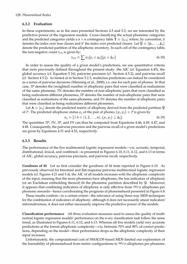
128 Phonemehood Redux
6.3.2 Evaluation
In these experiments, as in the ones presented Sections 4.5 and 5.2, we are interested by thepredictive power of the regression models. Cross-classifying the actual phonemic categoriesand the predicted categories yields a n× n contingency table T ≡ [th′h] where, by convention, hdenotes the index over true classes and h′ the index over predicted classes. Let P ≡ p1, . . . , pndenote the predicted partition of the allophonic inventory. In each cell of the contingency table,the non-negative count th′h is given by:
th′h ≡∑i
wiJpi ∈ phKJpi ∈ ph′K (6.18)
In order to assess the quality of a given model’s predictions, we use quantitative criteriathat were previously defined throughout the present study: the AIC (cf. Equation 4.45), theglobal accuracy (cf. Equation 5.16), pairwise precision (cf. Section 4.5.2), and pairwise recall(cf. Section 4.5.2). As hinted at in Section 5.2.3, multiclass predictions can indeed be consideredas a series of pairwise decisions (Manning et al., 2008), i.e. one for each pair of phones. In thatcase, TP denotes the (weighted) number of allophonic pairs that were classified as realizationsof the same phoneme, TN denotes the number of non-allophonic pairs that were classified asbeing realizations different phonemes, FP denotes the number of non-allophonic pairs that wereclassified as realizations of the same phoneme, and FN denotes the number of allophonic pairsthat were classified as being realizations different phonemes.
Let A ≡ [aij] denote the predicted matrix of allophony derived from the predicted partition Pof P. The predicted allophonic status aij of the pair of phones pi, pj ∈ P is given by
aij ≡ J∃ h ∈ (1, 2, . . . , n), pi, pj ⊆ phK. (6.19)The quantities TP, TN, FP, and FN can thus be computed from Equations 4.46, 4.49, 4.47, and4.48. Consequently, the pairwise precision and the pairwise recall of a given model’s predictionsare given by Equations 4.51 and 4.52, respectively.
6.3.3 Results
The performance of the five multinomial logistic regression models—viz. acoustic, temporal,distributional, lexical, and combined—is presented in Figures 6.10, 6.11, 6.12, and 6.13 in termsof AIC, global accuracy, pairwise precision, and pairwise recall, respectively.
Goodness of fit Let us first consider the goodness of fit tests reported in Figure 6.10. Aspreviously observed for binomial and flat-response pairwise multinomial logistic regressionmodels (cf. Figures 4.21 and 5.4), the AIC of all models increases with the allophonic complexityof the input, meaning that the more phonemes have allophones, the less indicators of allophony(or an Euclidean embedding thereof) fit the phonemic partition described by P. Moreover,it appears that combining indicators of allophony is only effective from 248/25 allophones perphoneme onwards—hence corroborating the prognosis of phonemehood presented in Figure 6.8.
These results confirm—to a certain extent—the relevance of using three-way MDS techniquesfor the combination of indicators of allophony: although it does not necessarily smear indicators’informativeness, it does not either necessarily improve the predictive power of the models.
Classification performance All three evaluation measures used to assess the quality of multi-nomial logistic regression models’ performance on the n-ary classification task follow the sametrend, as illustrated in Figures 6.11, 6.12, and 6.13. Whereas all five models yield very accuratepredictions at the lowest allophonic complexity—viz. between 70% and 90% of correct predic-tions, depending on the model—their performance drops as the allophonic complexity of theirinput increases.Unfortunately, the computational cost of SMACOF-based MDS limited our exploration of
the learnability of phonemehood from metric configurations to 588/25 allophones per phoneme.
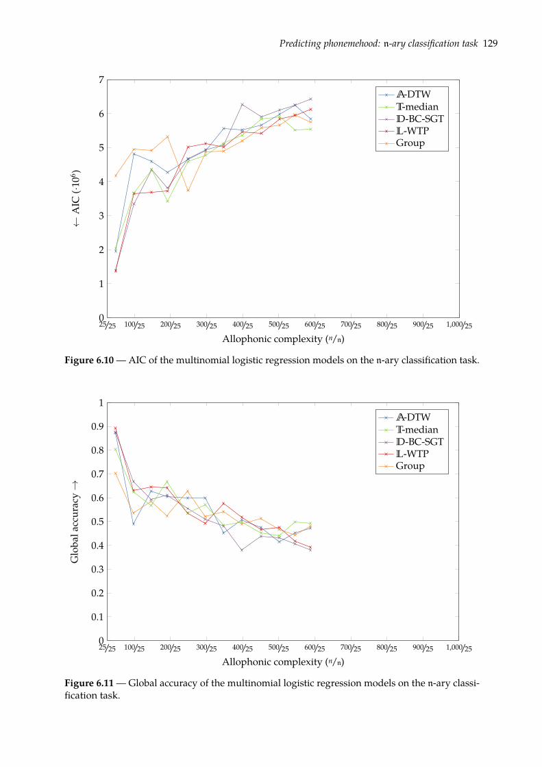
Predicting phonemehood: n-ary classification task 129
100/25 200/25 300/25 400/25 500/25 600/25 700/25 800/25 900/25 1,000/250
1
2
3
4
5
6
7
25/25
Allophonic complexity (n/n)
←A
IC(·1
06 )
A-DTWT-medianD-BC-SGTL-WTPGroup
Figure 6.10 — AIC of the multinomial logistic regression models on the n-ary classification task.
100/25 200/25 300/25 400/25 500/25 600/25 700/25 800/25 900/25 1,000/250
0.1
0.2
0.3
0.4
0.5
0.6
0.7
0.8
0.9
1
25/25
Allophonic complexity (n/n)
Glo
bala
ccur
acy→
A-DTWT-medianD-BC-SGTL-WTPGroup
Figure 6.11 — Global accuracy of the multinomial logistic regression models on the n-ary classi-fication task.
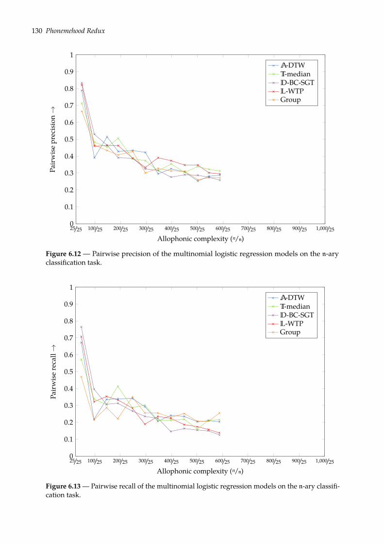
130 Phonemehood Redux
100/25 200/25 300/25 400/25 500/25 600/25 700/25 800/25 900/25 1,000/250
0.1
0.2
0.3
0.4
0.5
0.6
0.7
0.8
0.9
1
25/25
Allophonic complexity (n/n)
Pair
wis
epr
ecis
ion→
A-DTWT-medianD-BC-SGTL-WTPGroup
Figure 6.12 — Pairwise precision of the multinomial logistic regression models on the n-aryclassification task.
100/25 200/25 300/25 400/25 500/25 600/25 700/25 800/25 900/25 1,000/250
0.1
0.2
0.3
0.4
0.5
0.6
0.7
0.8
0.9
1
25/25
Allophonic complexity (n/n)
Pair
wis
ere
call→
A-DTWT-medianD-BC-SGTL-WTPGroup
Figure 6.13 — Pairwise recall of the multinomial logistic regression models on the n-ary classifi-cation task.
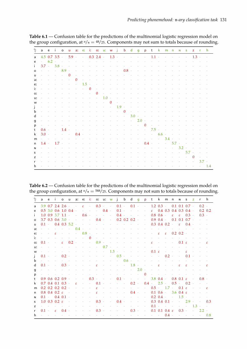
Predicting phonemehood: n-ary classification task 131
Table 6.1 — Confusion table for the predictions of the multinomial logistic regression model onthe group configuration, at n/n = 48/25. Components may not sum to totals because of rounding.
" a e i o u a: e: i: o: u: w j b d g p t k m n ð s z r h
a 4.5 0.7 3.5 - 5.9 - - 0.3 2.4 - 1.3 - - - - - 1.1 - - - - - 1.3 - -e - 6.2 - - - - - - - - - - - - - - - - - - - - - - -i 3.7 - 3.8 - - - - - - - - - - - - - - - - - - - - - -o - - - 8.9 - - - - - - - - 0.8 - - - - - - - - - - - -u - - - - 0 - - - - - - - - - - - - - - - - - - - -a: - - - - - 0 - - - - - - - - - - - - - - - - - - -e: - - - - - - 1.5 - - - - - - - - - - - - - - - - - -i: - - - - - - - 0 - - - - - - - - - - - - - - - - -o: - - - - - - - - 0 - - - - - - - - - - - - - - - -u: - - - - - - - - - 1.0 - - - - - - - - - - - - - - -w - - - - - - - - - - 0 - - - - - - - - - - - - - -j - - - - - - - - - - - 1.9 - - - - - - - - - - - - -b - - - - - - - - - - - - 0 - - - - - - - - - - - -d - - - - - - - - - - - - - 3.0 - - - - - - - - - - -g - - - - - - - - - - - - - - 2.0 - - - - - - - - - -p - - - - - - - - - - - - - - - 0 - - - - - - - - -t 0.6 - - 1.4 - - - - - - - - - - - - 7.5 - - - - - - - -k 3.0 - - - - 0.4 - - - - - - - - - - - 6.6 - - - - - - -m - - - - - - - - - - - - - - - - - - 3.4 - - - - - -n 1.4 - 1.7 - - - - - - - - - - - - 0.4 - - - 5.7 - - - - -ð - - - - - - - - - - - - - - - - - - - - 3.2 - - - -s - - - - - - - - - - - - - - - - - - - - - 5.7 - - -z - - - - - - - - - - - - - - - - - - - - - - 0 - -r - - - - - - - - - - - - - - - - - - - - - - - 3.7 -h - - - - - - - - - - - - - - - - - - - - - - - - 1.4
Table 6.2 — Confusion table for the predictions of the multinomial logistic regression model onthe group configuration, at n/n = 588/25. Components may not sum to totals because of rounding.
" a e i o u a: e: i: o: u: w j b d g p t k m n ð s z r h
a 3.9 0.7 2.4 2.6 - - ε - 0.3 - - 0.1 - 0.1 - - 1.2 0.3 - 0.1 0.1 0.7 - 0.2 -e 0.5 3.0 0.6 1.0 0.4 - - - - 0.4 - 0.1 - - - - ε 0.4 0.3 0.4 0.3 0.4 - 0.2 0.2i 1.0 0.9 3.7 1.1 - - 0.6 - - - - 0.4 - - - - 0.8 0.6 - ε ε 0.3 - 0.3 -o 3.7 0.3 0.6 3.0 - - - - 0.4 - - 0.2 0.2 0.2 - - 0.9 0.4 - 0.1 0.1 0.7 - - -u 0.1 - 0.4 0.3 5.2 - - - - - - - - - - - 0.3 0.4 0.2 - ε 0.4 - - -a: - - - - - 0.4 - - - - - - - - - - - - - - - - - - -e: - - ε - - - 0.8 - - - - - - - - - - ε ε 0.2 0.2 - - - -i: - - - - - - - 0 - - - - - - - - - - - - - - - - -o: 0.1 - - ε 0.2 - - - 0.9 - - - - - - - ε - - - 0.1 ε - - εu: - - - - - - - - - 0.7 - - - - - - - - - - - - - - -w - - - - - - - - - - 1.3 - - - - - 0.1 ε - - - ε - - -j 0.1 - - 0.2 - - - - - - - 0.5 - - - - - - 0.2 - - 0.1 - - -b - - - - - - - - - - - - 0.6 - - - - - - - - - - - -d 0.1 - - 0.3 - - - - ε - - - - 1.8 - - - ε - - ε ε - - εg - - - - - - - - - - - - - - 2.0 - - - - - - - - - -p - - - - - - - - - - - - - - - 0 - - - - - - - - -t 0.9 0.6 0.2 0.9 - - - 0.3 - - - 0.1 - - - - 3.8 0.4 - 0.8 0.1 ε - 0.8 -k 0.7 0.4 0.1 0.3 - ε - - 0.1 - - - - 0.2 - 0.4 - 2.5 - 0.5 - 0.2 - - -m 0.2 0.2 0.2 0.2 - - - - ε - - - - - - - 0.5 - 1.7 - 0.1 ε - - εn 0.8 0.4 0.2 ε - - - - ε - - - - 0.4 - - 0.1 0.6 - 3.6 0.4 ε - - -ð 0.1 - 0.4 0.1 - - - - - - - - - - - - 0.2 0.4 - - 1.5 - - - -s 1.0 0.3 0.2 ε - - - - 0.3 - - 0.4 - - - - 0.3 0.4 0.1 - - 2.9 - - 0.3z - - - - - - - - - - - - - - - - 0.1 - - - - - 1.3 - -r 0.1 - ε 0.4 - - - - 0.3 - - - - 0.3 - - 0.1 0.1 0.4 ε 0.3 - - 2.2 -h - - - - - - - - - - - - - - - - - - 0.4 - - - - - 0.8
132 Phonemehood Redux
We are thus unable to assess whether the performance of our models keeps decreasing as theallophonic complexity of the input increases, or if it plateaus from 588/25 allophones per phonemeonwards—as observed, for example, in Figures 5.7 and 5.7, for the (n+1)-ary classification tasks.Finally, it is worth noting that Figures 6.11, 6.12, and 6.13 appear to be chaotic, as no definite
pattern emerges regarding the identity of the optimal model, and the least performant modelat a given allophonic complexity may well be the most performant one at the next complexity.We speculate that this is due to our (forced) choice to end the optimization process of eachmetric configuration after 100 SMACOF iterations—regardless of the concurrent gain in stress.Discussing the relative influence of SMACOF’s convergence criteria is an issue we leave as arecommendation for future research.
Contingency tables For the sake of illustration, we report the contingency tables obtainedfor the combined model at minimal and maximal allophonic complexities in Tables 6.1 and6.2, respectively. At 48/25 allophones per phoneme, all allophones of 12 out of 25 phonemes(in green in the table header) are perfectly classified. By contrast, not a single allophone of 8out of 25 phonemes was correctly classified (in red in the table header). Moreover, is is worthnoting that misclassifications tend to consist in phones being predicted as being realizationsof the most frequent phonemes in Japanese, viz. /a/, /i/, /o/, /t/, /k/, and /n/, as observed inSection 5.2.4. In other words, /a/ is the new ⊗. The figures reported in Table 6.2 confirm thatthis frequency-magnet effect still occurs at 588/25 allophones per phoneme, as the same frequentphonemes account for most misclassifications.
All things considered, these results indicate that aggregating all phones in a given allophonicinventory into phoneme-like categories is not an easy task—even in a best-case scenario werelabeled data is available (logistic regression is a supervised technique) and confirmatory overfit-ting is conducted. We can thus be but skeptical as to the learnability of phonemehood from thesame data (and representation thereof), but in a unsupervised setup.
6.4 Predicting phonemehood: ?-ary clustering task
Up to this point, all experiments reported in this dissertation consisted in supervised learningtechniques—actually variations on a single technique, i.e. logistic regression. However, from theperspective of early language acquisition, no labeled data should be available to the learner. Theexperiments we present in this section aim at assessing whether compact and well-separatedclusters can be inferred from the indicators’ metric configurations. As emphasized by Höppner(2009; p. 386):
We are not interested in artificially dividing the [objects] into similar groups, but we wantto know if the data itself supports a partition into different groups,~
hence the jocular arity in the title of this section.
Definitions and objectives Clustering—a classic approach to unsupervised learning—refers tothe problemof trying to find hidden structure in unlabeled data (e.g. Jain et al., 1999;Mirkin, 2005).In the case at hand, we aim at partitioning the allophonic inventory P into a set Ω ≡ ω1, . . . , ωηof η collectively exhaustive and mutually exclusive clusters. As previously discussed throughoutthe present study, the optimal partition of any given allophonic inventory P is the phonemicinventory P of the language at hand. Moreover, the quality of the clustering solution Ω isbounded by the following limiting cases (Reichart & Rappoport, 2009): the single cluster solution,whereby all phones are assigned to the same unique cluster, i.e.
Ω = P, (6.20)and the singletons solution, whereby each phone is assigned to a cluster of its own, i.e.
Ω = pi : pi ∈ P. (6.21)
Predicting phonemehood: ?-ary clustering task 133
Furthermore, we refer to a partition whereby each cluster contains only allophones as beinghomogeneous, and to a partition whereby, for each phoneme, all its allophones are assigned to thesame cluster as being complete (Meila, 2007; Rosenberg &Hirschberg, 2007; Reichart & Rappoport,2009). Consequently, whereas the single cluster solution is only complete and the singletonssolution is only homogeneous, the reference phonemic partition P is both fully homogeneousand fully complete.
6.4.1 Density-based clustering with DBSCAN
In order to assess whether the data at hand supports a partition into different groups, we usethe DBSCAN algorithm (Ester et al., 1996), a classic density-based clustering algorithm that isable to discover clusters of arbitrary shapes. Whereas other density-based clustering algorithmshave been proposed (e.g. CLARANS; Ng & Han, 1994), DBSCAN’s main attraction arises fromits efficiency on large datasets, as its average time complexity is in O(n log2 n).Another remarkable property of DBSCAN is that this algorithm does not require locations
estimates, but only object-to-object dissimilarities. In the case at hand, this property allows forthe comparison of clustering solutions obtained for both the original dissimilarities and thecomputed Euclidean distances. In this section, let ∆ ≡ [δij] denote the input dissimilarity ordistance matrix, regardless of its true nature. The original formulation of DBSCAN does notaccommodate weighted objects. For this reason, we hereby give a detailed presentation of theweighted extension of DBSCAN we propose, emphasizing the discrepancies with Ester et al.’s(1996) formulation.
Density-based clustering The notion of spatial density in DBSCAN resembles the notion ofpopulation density in demographic studies, in the sense that it is defined as a combination ofpopulation and volume: given objects must be close enough and numerous enough in order toform a dense cluster. In DBSCAN, density is further defined by two parameters, viz. ε ∈ R+
which controls how far two points can be so that they may still be assigned to the same cluster,and φ ∈N which controls how many close-enough points are required to start a cluster.One of the two major concepts shared by DBSCAN and its extensions is the ε-neighborhood
of an object. Using Kailing et al.’s (2004b) notation, let N ∆ε (pi) denote the ε-neighborhood of a
given phone pi ∈ P with respect to the representation ∆. The ε-neighborhood of pi is defined asthe set of objects whose distance to pi is less than or equal to ε, i.e.
N ∆ε (pi) ≡
pj ∈ P : δij ≤ ε
. (6.22)
It is worth highlighting that, according to this definition, any object belongs to its own ε-neighborhood.The other major concept allowing for the definition of density in DBSCAN is core objects. In
the original formulation of the algorithm, a core object with respect to ∆, ε, and φ was definedas an object whose ε-neighborhood contains at least φ other phones, that is
core(pi; ∆, ε, φ) ≡q
φ ≤ |N ∆ε (pi)|
y. (6.23)
In the case at hand, we amend this definition so that each phone’s instance weight impacts thecomputation of the density in its vicinity. One solution would consist in replicating wi timesthe point mi representing a given phone pi ∈ P. However, this solution is not desirable at thetime complexity of the clustering procedure would thus be in O(∑i wi log2 ∑i wi)—rather thanin O(n log2 n). In our weighted extension of DBSCAN, a core object with respect to ∆, w, ε, andφ is therefore defined as an object whose ε-neighborhood weighs at least φ, i.e.
core(pi; ∆, w, ε, φ) ≡t
φ ≤ ∑pj ∈N ∆
ε (pi)
wj
|
(6.24)
It is worth noting that the latter definition is similar to the weight function used in Sander et al.’s(1998) density-based clustering algorithm.
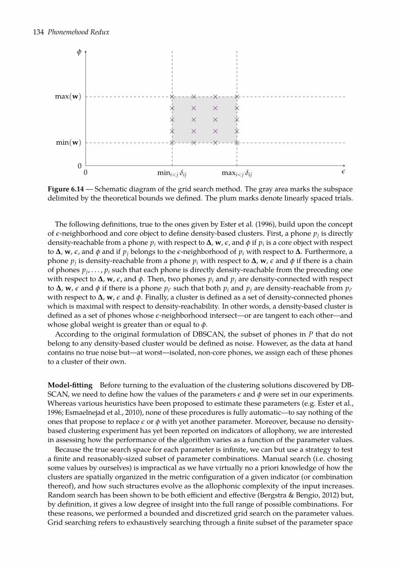
134 Phonemehood Redux
0 mini<j δij maxi<j δij ε0
min(w)
max(w)
φ
×××××
×××××
×××××
×××××
Figure 6.14 — Schematic diagram of the grid search method. The gray area marks the subspacedelimited by the theoretical bounds we defined. The plum marks denote linearly spaced trials.
The following definitions, true to the ones given by Ester et al. (1996), build upon the conceptof ε-neighborhood and core object to define density-based clusters. First, a phone pj is directlydensity-reachable from a phone pi with respect to ∆, w, ε, and φ if pi is a core object with respectto ∆, w, ε, and φ and if pj belongs to the ε-neighborhood of pi with respect to ∆. Furthermore, aphone pj is density-reachable from a phone pi with respect to ∆, w, ε and φ if there is a chainof phones pj, . . . , pi such that each phone is directly density-reachable from the preceding onewith respect to ∆, w, ε, and φ. Then, two phones pi and pj are density-connected with respectto ∆, w, ε and φ if there is a phone pi′ such that both pi and pj are density-reachable from pi′
with respect to ∆, w, ε and φ. Finally, a cluster is defined as a set of density-connected phoneswhich is maximal with respect to density-reachability. In other words, a density-based cluster isdefined as a set of phones whose ε-neighborhood intersect—or are tangent to each other—andwhose global weight is greater than or equal to φ.
According to the original formulation of DBSCAN, the subset of phones in P that do notbelong to any density-based cluster would be defined as noise. However, as the data at handcontains no true noise but—at worst—isolated, non-core phones, we assign each of these phonesto a cluster of their own.
Model-fitting Before turning to the evaluation of the clustering solutions discovered by DB-SCAN, we need to define how the values of the parameters ε and φ were set in our experiments.Whereas various heuristics have been proposed to estimate these parameters (e.g. Ester et al.,1996; Esmaelnejad et al., 2010), none of these procedures is fully automatic—to say nothing of theones that propose to replace ε or φ with yet another parameter. Moreover, because no density-based clustering experiment has yet been reported on indicators of allophony, we are interestedin assessing how the performance of the algorithm varies as a function of the parameter values.Because the true search space for each parameter is infinite, we can but use a strategy to test
a finite and reasonably-sized subset of parameter combinations. Manual search (i.e. chosingsome values by ourselves) is impractical as we have virtually no a priori knowledge of how theclusters are spatially organized in the metric configuration of a given indicator (or combinationthereof), and how such structures evolve as the allophonic complexity of the input increases.Random search has been shown to be both efficient and effective (Bergstra & Bengio, 2012) but,by definition, it gives a low degree of insight into the full range of possible combinations. Forthese reasons, we performed a bounded and discretized grid search on the parameter values.Grid searching refers to exhaustively searching through a finite subset of the parameter space
Predicting phonemehood: ?-ary clustering task 135
(e.g. Hsu et al., 2010), as illustrated in Figure 6.14. It is reliable in low-dimensional parameterspaces—as in the case at hand, where we have 2 parameters—and, from a technical perspective,it is simple to implement and parallelization is trivial (Bergstra & Bengio, 2012).
It order to guarantee the tractability and the relevance of our experiments, we first define, foreach parameter ε and φ, a range of relevant values to be tested. To our knowledge, the followinga priori bounds have never been described, neither for DBSCAN nor for derivatives thereof(Ester et al., 1996; Sander et al., 1998; Ankerst et al., 1999; Wang & Hamilton, 2003; Wang et al.,2004; Kailing et al., 2004a,b; Gorawski & Malczok, 2006a,b; Ruiz et al., 2007)—it is worth noting,however, that Esmaelnejad et al.’s (2010) heuristic for setting the value of ε has a similar rationale.
As aforestated, ε ∈ R+ controls how far two phones can be so that they may still be assignedto the same cluster. Thus, it mostly interacts with the distances or dissimilarities in ∆. Ifε < mini<j δij, no two phones are ε-reachable and, hence, each phone’s ε-neighborhood isreduced to the phone itself and the clustering solution can not be better than the singletonssolution. If ε = maxi<j δij, then the farthest phones are ε-reachable. Thus, all other things beingequal, clustering with ε > maxi<j δij can not yield better solutions than the one obtained withε = maxi<j δij. The relevant range of values for ε is hence bounded by the attested range ofdistance or dissimilarity values in ∆:
mini<j
δij ≤ ε ≤ maxi<j
δij. (6.25)
On the other hand, φ ∈N controls howmany close-enough phones are required to start a cluster.Thus, it mostly interacts with the weights in w to select core objects. The minimum weight ofall phones’ ε-neighborhoods is min(w). Therefore, all other things being equal, clustering withφ < min(w) can not yield clustering solutions different than the one obtained with φ = min(w).Similarly, if φ > max(w), then no phone can be a core object and no clustering solution can bedifferent from the singletons solutions. The relevant range of values for φ is hence bounded bythe attested range of distance or dissimilarity values in w:
min(w) ≤ φ ≤ max(w). (6.26)Relying on these a priori bounds on the parameters ε and φ, we tested 100 linearly-spaced
values for each parameter, i.e. we performed a grid search over 1002 = 10, 000 DBSCAN trialsfor each indicator of allophony (or combination thereof), and for each allophonic complexity.
6.4.2 Evaluation
Because providing a thorough examination of thousands of clustering solutions is unfeasible—ifrelevant at all—we only report the performance of DBSCAN for the optimal clustering solutioncomputed for each indicator and allophonic complexity.
Contingency table Cross-classifying a given clustering solution Ω and the reference phonemicpartition P yields an η × n contingency table T ≡ [toh] where o ∈ (1, 2, . . . , η) denotes the indexover the predicted clusters, and h ∈ (1, 2, . . . , n) denotes the index over the phonemes of thetarget language. In each cell, the non-negative count toh is given by the (weighted) number ofallophones of ph that were assigned to the cluster ωo, i.e.
toh ≡∑i
wiJpi ∈ phKJpi ∈ ωoK. (6.27)
Objective function The quantitative criterion we use as the objective function to retrieve theoptimal clustering solution in the grid search is known as the normalized variation of information(henceforth NVI; Reichart & Rappoport, 2009). NVI is an information-theoretic measure givenby:
NVI(Ω;P) ≡
H(P | Ω) + H(Ω | P)
H(P)if H(P) 6= 0
H(Ω) otherwise(6.28)
136 Phonemehood Redux
where
H(P) ≡ −∑h
[∑o toh
∑i wilog2
∑o toh
∑i wi
], (6.29)
H(P | Ω) ≡ −∑o
∑h
[toh
∑i wilog2
toh
∑′h toh
], (6.30)
H(Ω) ≡ −∑o
[∑h toh
nlog2
∑h toh
∑i wi
], (6.31)
H(Ω | P) ≡ −∑o
∑h
[toh
∑i wilog2
toh
∑′o toh
]. (6.32)
Although discussing the rationale of the computation of NVI is beyond the scope of this dis-sertation, it is worth highlighting that NVI values decrease as the clustering solution becomesmore complete and more homogeneous and, hence, that the reference phonemic partition Phas a NVI equal to 0. For each indicator of allophony (or combination thereof) and allophoniccomplexity, the optimal clustering solution is thus the one that minimizes the NVI. Moreover,the single cluster solution has a NVI equal to 1. Although Reichart & Rappoport (2009) give noupper bound for NVI, they indicate that all clustering solutions of higher quality than the singlecluster solution are scored by NVI in the range [0, 1].Because NVI is an external cluster validity index, one could object that performing a grid
search whose objective function relies on the reference clustering solution—i.e. P—is akin toperforming supervised learning. It is however worth noting that each DBSCAN trial is trulyunsupervised. Furthermore, in light of the results presented in Sections 6.2 and 6.3, we knowthat none of the metric configurations we computed from our indicators of allophony supports acomplete and homogeneous phonemic partition of the allophonic inventories. The results to befurther reported in this section are thus the best among the worst.
Purity For the sake of comparability with previously reported experiments in this study, wealso use other evaluation measures to assess the quality of the density-based clustering solutions.Whereas accuracy is only relevant in supervised learning setups—i.e. when each predictedcategory can be matched to a reference category—purity can be interpreted as its unsupervisedcounterpart (Manning et al., 2008). To compute the purity of a clustering solution, each cluster isassigned to the phoneme which is most frequent in the cluster, and then the accuracy of thisassignment is measured by counting the (weighted) number of correctly assigned phones anddividing by the number of phones. Formally, we have:
purity(T) ≡ 1∑i wi
∑o
(max
htoh
)(6.33)
From this definition, one can easily see that purity values lie in [0, 1]: bad clustering solutionshave purity values close to 0, and the reference phonemic partition P has a purity of 1. Asemphasized by (Reichart&Rappoport, 2009), purity evaluates homogeneity, but does not evaluatecompleteness at all. Whereas the purity of the singletons solutions is, by definition, equal to 1,the purity of the single cluster solution depends on the dataset at hand. More precisely, it isgiven by the ratio of the frequency of the most frequent phoneme to the sum of all phonemes’frequency, i.e.
maxh ∑i wiJpi ∈ phK∑i wi
=2125541591966
≈ 0.13 (6.34)
Pairwise evaluation As with any multiclass problem, the predictions can be considered as aseries of pairwise decision. Using the same rationale as in Section 6.3, the quantities TP, TN, FP,
Predicting phonemehood: ?-ary clustering task 137
and FN are given by
TP ≡∑h, o
(tho
2
)(6.35)
FP ≡ −TP + ∑h
(∑o tho
2
)(6.36)
FN ≡ −TP + ∑o
(∑h tho
2
)(6.37)
TN ≡(
∑h, o tho
2
)− TP− FP− FN (6.38)
Consequently, the pairwise precision and the pairwise recall of a given model’s predictions aregiven by Equations 4.51 and 4.52, respectively.
6.4.3 Results
The performance of the density-based clustering model on all aforementioned metric configu-rations is presented in Figures 6.16, 6.17, 6.18, and 6.19 in terms of NVI, purity, precision, andrecall, respectively.
Grid search Let us first consider the results of the grid searches, as illustrated in Figure 6.15where—for the sake of brevity—we only present the surface responses for a subset of the testedallophonic complexities. For each model and allophonic complexity, the surface response is agraphical representation of the result of the corresponding grid search whereby the observedNVI values for all tested parameter values are cross-classified. NVI values are mapped to alinear grayscale whereby values equal to 0 are mapped to black and values greater than or equalto 1 to white. Because NVI is to be minimized, dark areas thus indicate effective parametercombinations.
All surface response call for a general observation: the value of ε is irrelevant for the purposeof clustering any given allophonic inventory into a phoneme-like partition. Indeed, if it is notcompletely blank, each response surface shows a horizontal pattern, meaning that only theparameter on the y-axis (i.e. φ) has an impact on the quality of the clustering solution. Because φmostly interacts with the weights in w, this result corroborates—once again—the influence ofthe frequency-based instance weights on the discovery of phonemes.Another interesting observation is that, except for the acoustic indicator, the 30-dimensional
metric configurations appear to yield better density-based clustering solutions than the corre-sponding original dissimilarities. Whereas a dark horizontal pattern appears, for instance, in theresponse surfaces for themetric configurations of the distributional and lexical indicators, the cor-responding response surfaces for their original dissimilarities are completely blank—regardlessof the allophonic complexity of their input. By contrast, Figure 6.15 suggests that the effective-ness of the acoustic indicator for the discovery of phonemes suffers—to some extent—fromthe Euclidean embedding, as the corresponding response surfaces fade to white as allophoniccomplexity increases. This result is important in itself, and we consider it to be a validation of ourMDS-based reformulation of Peperkamp et al.’s (2006) framework. Indeed, the response surfacespresented in Figure 6.15 show that embedding indicators of allophony in a multidimensionalEuclidean space does not smear the information they contain—to say nothing of the availabilityof three-way extension allowing for the combinations of various indicators.
Clustering quality All other evaluation measures give a similar assessment of the quality ofthe density-based phoneme-like clustering solutions, as illustrated in Figures 6.16, 6.17, 6.18, and6.19. Except for the acoustic indicator, DBSCAN always outputs the singletons solution, i.e. thelimiting case whereby each phone in the allophonic inventory is assigned to its own cluster.
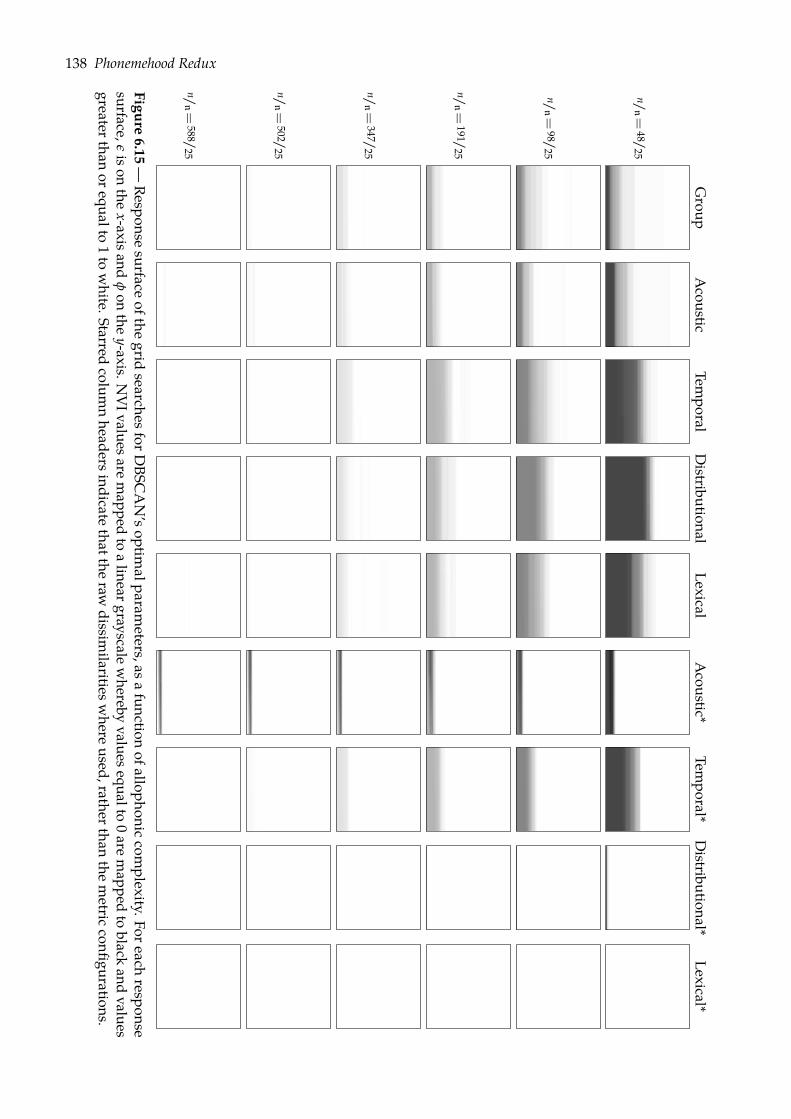
138 Phonemehood Redux
Group
Acoustic
Temporal
Distributional
LexicalAcoustic*
Temporal*
Distributional*
Lexical*
n/n=
48/25
n/n=
98/25
n/n=
191/25
n/n=
347/25
n/n=
502/25
n/n=
588/25
Figure6.15
—Response
surfaceofthe
gridsearchesforD
BSCAN’soptim
alparameters,asa
functionofallophonic
complexity.Foreach
responsesurface,
εison
thex-axisand
φon
they-axis.N
VIvaluesare
mapped
toalineargrayscale
whereby
valuesequalto0are
mapped
toblack
andvalues
greaterthanorequalto
1to
white.Starred
columnheadersindicate
thattheraw
dissimilaritiesw
hereused,ratherthan
themetric
configurations.
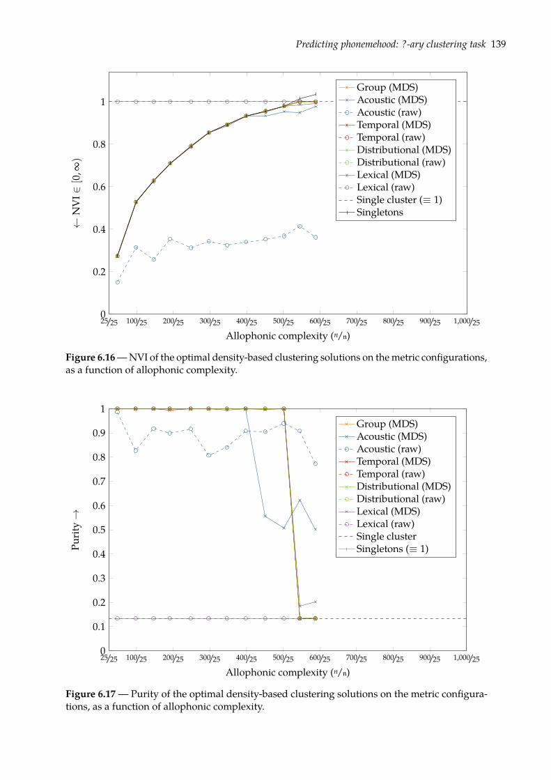
Predicting phonemehood: ?-ary clustering task 139
100/25 200/25 300/25 400/25 500/25 600/25 700/25 800/25 900/25 1,000/250
0.2
0.4
0.6
0.8
1
25/25
Allophonic complexity (n/n)
←N
VI∈
[0,∞
)Group (MDS)Acoustic (MDS)Acoustic (raw)Temporal (MDS)Temporal (raw)Distributional (MDS)Distributional (raw)Lexical (MDS)Lexical (raw)Single cluster (≡ 1)Singletons
Figure 6.16—NVI of the optimal density-based clustering solutions on themetric configurations,as a function of allophonic complexity.
100/25 200/25 300/25 400/25 500/25 600/25 700/25 800/25 900/25 1,000/250
0.1
0.2
0.3
0.4
0.5
0.6
0.7
0.8
0.9
1
25/25
Allophonic complexity (n/n)
Purit
y→
Group (MDS)Acoustic (MDS)Acoustic (raw)Temporal (MDS)Temporal (raw)Distributional (MDS)Distributional (raw)Lexical (MDS)Lexical (raw)Single clusterSingletons (≡ 1)
Figure 6.17 — Purity of the optimal density-based clustering solutions on the metric configura-tions, as a function of allophonic complexity.
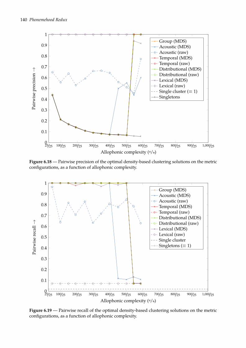
140 Phonemehood Redux
100/25 200/25 300/25 400/25 500/25 600/25 700/25 800/25 900/25 1,000/250
0.1
0.2
0.3
0.4
0.5
0.6
0.7
0.8
0.9
1
25/25
Allophonic complexity (n/n)
Pair
wis
epr
ecis
ion→
Group (MDS)Acoustic (MDS)Acoustic (raw)Temporal (MDS)Temporal (raw)Distributional (MDS)Distributional (raw)Lexical (MDS)Lexical (raw)Single cluster (≡ 1)Singletons
Figure 6.18— Pairwise precision of the optimal density-based clustering solutions on the metricconfigurations, as a function of allophonic complexity.
100/25 200/25 300/25 400/25 500/25 600/25 700/25 800/25 900/25 1,000/250
0.1
0.2
0.3
0.4
0.5
0.6
0.7
0.8
0.9
1
25/25
Allophonic complexity (n/n)
Pair
wis
ere
call→
Group (MDS)Acoustic (MDS)Acoustic (raw)Temporal (MDS)Temporal (raw)Distributional (MDS)Distributional (raw)Lexical (MDS)Lexical (raw)Single clusterSingletons (≡ 1)
Figure 6.19 — Pairwise recall of the optimal density-based clustering solutions on the metricconfigurations, as a function of allophonic complexity.
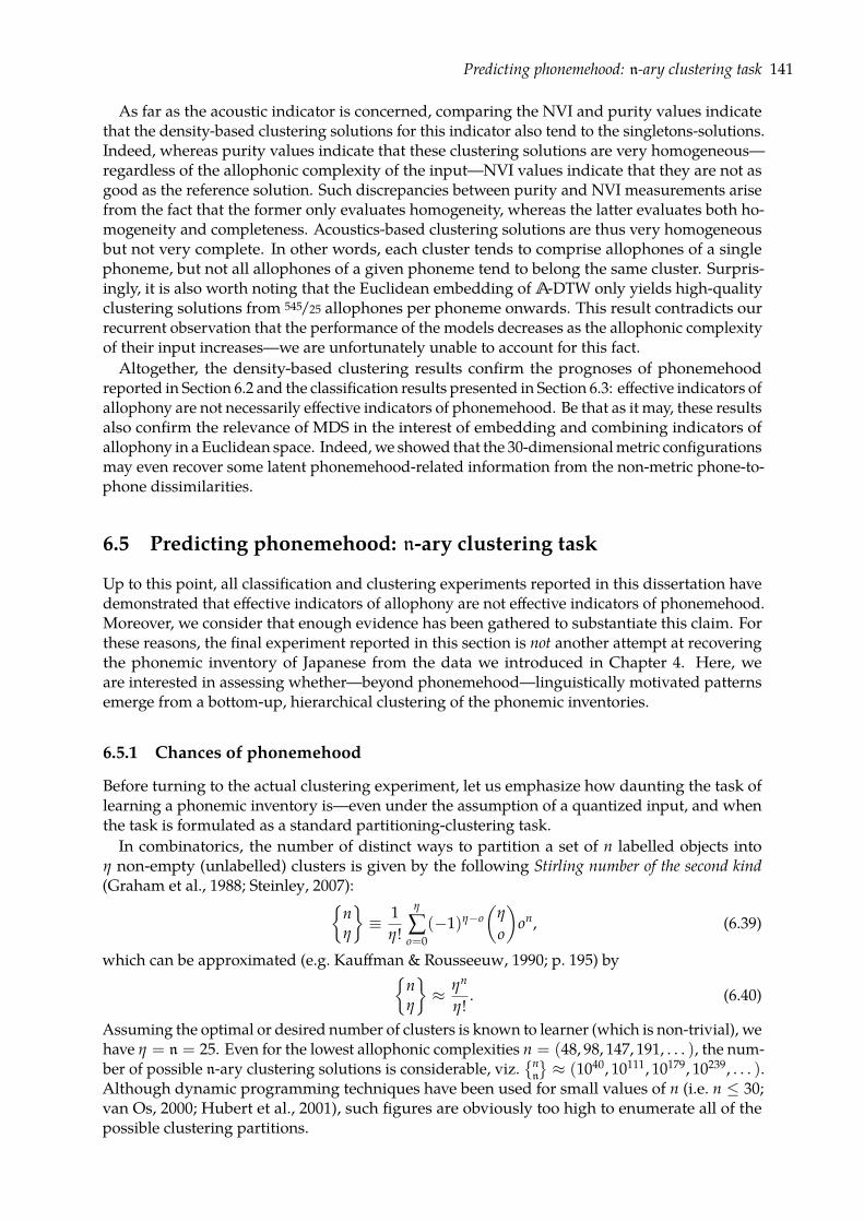
Predicting phonemehood: n-ary clustering task 141
As far as the acoustic indicator is concerned, comparing the NVI and purity values indicatethat the density-based clustering solutions for this indicator also tend to the singletons-solutions.Indeed, whereas purity values indicate that these clustering solutions are very homogeneous—regardless of the allophonic complexity of the input—NVI values indicate that they are not asgood as the reference solution. Such discrepancies between purity and NVI measurements arisefrom the fact that the former only evaluates homogeneity, whereas the latter evaluates both ho-mogeneity and completeness. Acoustics-based clustering solutions are thus very homogeneousbut not very complete. In other words, each cluster tends to comprise allophones of a singlephoneme, but not all allophones of a given phoneme tend to belong the same cluster. Surpris-ingly, it is also worth noting that the Euclidean embedding of A-DTW only yields high-qualityclustering solutions from 545/25 allophones per phoneme onwards. This result contradicts ourrecurrent observation that the performance of the models decreases as the allophonic complexityof their input increases—we are unfortunately unable to account for this fact.Altogether, the density-based clustering results confirm the prognoses of phonemehood
reported in Section 6.2 and the classification results presented in Section 6.3: effective indicators ofallophony are not necessarily effective indicators of phonemehood. Be that as it may, these resultsalso confirm the relevance of MDS in the interest of embedding and combining indicators ofallophony in a Euclidean space. Indeed, we showed that the 30-dimensionalmetric configurationsmay even recover some latent phonemehood-related information from the non-metric phone-to-phone dissimilarities.
6.5 Predicting phonemehood: n-ary clustering task
Up to this point, all classification and clustering experiments reported in this dissertation havedemonstrated that effective indicators of allophony are not effective indicators of phonemehood.Moreover, we consider that enough evidence has been gathered to substantiate this claim. Forthese reasons, the final experiment reported in this section is not another attempt at recoveringthe phonemic inventory of Japanese from the data we introduced in Chapter 4. Here, weare interested in assessing whether—beyond phonemehood—linguistically motivated patternsemerge from a bottom-up, hierarchical clustering of the phonemic inventories.
6.5.1 Chances of phonemehood
Before turning to the actual clustering experiment, let us emphasize how daunting the task oflearning a phonemic inventory is—even under the assumption of a quantized input, and whenthe task is formulated as a standard partitioning-clustering task.In combinatorics, the number of distinct ways to partition a set of n labelled objects into
η non-empty (unlabelled) clusters is given by the following Stirling number of the second kind(Graham et al., 1988; Steinley, 2007):
nη
≡ 1
η!
η
∑o=0
(−1)η−o(
η
o
)on, (6.39)
which can be approximated (e.g. Kauffman & Rousseeuw, 1990; p. 195) by
nη
≈ ηn
η!. (6.40)
Assuming the optimal or desired number of clusters is known to learner (which is non-trivial), wehave η = n = 25. Even for the lowest allophonic complexities n = (48, 98, 147, 191, . . . ), the num-ber of possible n-ary clustering solutions is considerable, viz.
nn
≈ (1040, 10111, 10179, 10239, . . . ).
Although dynamic programming techniques have been used for small values of n (i.e. n ≤ 30;van Os, 2000; Hubert et al., 2001), such figures are obviously too high to enumerate all of thepossible clustering partitions.
142 Phonemehood Redux
When the number of cluster is unknown, the number of distinct ways to partition a set of nlabelled objects into non-empty (unlabelled) clusters is known as the n-th Bell number, denotedBn. Such a number is defined as the sum of all Stirling numbers of the second kind from 0 to n(Graham et al., 1988; p. 359), i.e.
Bn ≡n
∑η=0
nη
. (6.41)
One can easily see from this last equation that such figures grow even faster than the correspond-ing Stirling numbers.The purpose of this brief analysis is to emphasize the fact that partitioning-clustering—and,
generally speaking, unsupervised learning—is a hard task. Throughout the present study, wehave further assumed that only one partition is correct, viz. P. Consequently, for the lowestallophonic complexities n = (48, 98, 147, 191, . . . ), the odds of randomly discovering the phone-mic partition are virtually null, viz.
nn
−1 ≈ (10−40, 10−111, 10−179, 10−239, . . . ). In light of theaforestated prognosis, classification, and clustering results, we can assert that the data at hand(i.e. acoustic, temporal, distributional, and lexical indicators) are simply insufficient for theacquisition of phonemes.
n-means clustering algorithm It is worth noting that we did, however, perform additionalpartitioning-clustering experiments, using the seminal K-means clustering algorithm (algorithmby Lloyd, 1957; Forgy, 1965; MacQueen, 1967; and Hartigan &Wong, 1979; implementation byPardo & DelCampo, 2007), and setting the desired number of clusters K to the true number ofphonemes n. As emphasized by Mirkin (2005),
[the underlying model is] based on the somewhat simplistic claim that entities can berepresented by their cluster’s centroids, up to residuals.~
Although provided with the optimal number of clusters, n-means clustering is indeed simplisticto discover the phonemic inventory of the target language. Compared to the previously reporteddensity-based clustering experiments, the use of n-means yielded no significantly differentresults, which—for the sake of brevity—are not reported here.
6.5.2 Complete-linkage hierarchical clustering
In order to assess whether linguistically relevant patterns, e.g. the pervasive consonants vs.vowels dichotomy, may emerge from our data, we performed agglomerative (i.e. bottom-up)hierarchical clustering on the metric configurations.
Agglomerative clustering Hierarchical clustering techniques differ from partitioning-clustering techniques in the sense that the clustering solution the former techniques output donot consist in a partition of the input data, but in a dendrogram—a tree structure whose leavescontains the input objects, and whose branching nodes are to be interpreted as traces of thesuccessive clustering decisions (splits or merges) taken to produce the tree.As far as agglomerative clustering is concerned, all techniques start from the singletons
solutions, i.e.Ω = pi : pi ∈ P. (6.42)
Clusters are then iteratively merged until only one large cluster remains which contains allthe observations (R Development Core Team, 2010; cf. stats::hclust). At each stage, the twonearest clusters in Ω are combined to form one larger cluster. In this context, various formaldefinitions of the word nearest—referred to as linkage functions—are possible. We hereby brieflyreview the most popular linkage functions.The most intuitive linkage function is known as single-linkage, and is given by
linkage(ω, ω′; M) ≡ min
dij(M) : pi ∈ ω, pj ∈ ω′
. (6.43)
Predicting phonemehood: n-ary clustering task 143
This strategy is to be interpreted as a friends-of-friends approach whereby the distance betweentwo clusters is computed as the distance between the two closest phones in the two clusters.An undesirable side-effect of using single-linkage—referred to as the chaining effect—is thatclusters may be forced to merge due to single phones being close to one another, even if mostphones in each cluster are very distant to each other (e.g. Lupşa, 2005; Manning et al., 2008).
Ward’s criterion is another classic linkage function (Ward, 1963; Mirkin, 2005). Formally,Ward’s criterion between two clusters is given by
linkage(ω, ω′; M) ≡ |ω| |ω′||ω|+ |ω′| d
(ω, ω′
)where ω ≡ 1
|ω| ∑pi∈ω
mi. (6.44)
It is worth noting, however, that using this linkage function is unsuitable in the case at hand,as it relies on the centroids ω and ω′. We have indeed shown in Sections 6.2 and 6.3 that ourdata violate the compactness hypothesis, as the true phonemic clusters are neither compact norwell-separated. This approach would thus suffer the same limitations as K-means (Mirkin, 2005).
Finally, the linkage function we use in this experiment is known as the complete-linkage. Inthis approach to agglomerative clustering, the distance between two clusters is computed as thedistance between the two farthest phones in the two clusters, i.e.
linkage(ω, ω′; M) ≡ max
dij(M) : pi ∈ ω, pj ∈ ω′
. (6.45)Complete-linkage tends to produce tightly bound clusters and, to our knowledge, has no knownundesirable side-effect (Lupşa, 2005).
Phonemic cut Hierarchical clustering techniques yield dendrograms with as many leaves asthere are phones in the input allophonic inventory. For the sake of simplicity, we therefore cuteach dendrogram so as to obtain a canopy-clustered dendrogram with n = 25 leaves only.
6.5.3 Evaluation
For the purpose of the present analysis, no quantitative criteria appeared to be appropriate. Wetherefore limited the evaluation of the hierarchical clustering solutions to a visual examination ofthe output dendrograms. Because such dendrograms are space-consuming data representations,we further limited our examination to the group configurations of the combined model.
6.5.4 Results
The resulting dendrograms for the group configurations are presented in Figures 6.20, 6.21,6.22, 6.23, 6.24, and 6.25 at allophonic complexities of 48/25, 98/25, 191/25, 347/25, 502/25, and 588/25
allophones per phoneme, respectively. In each dendrogram, branches are ordered so that, foreach internal node, the tighter cluster is on the left. Subscript figures indicate, for each phoneme,the percentage of its (weighted) occurrences falling in that cluster; ε denotes quantities less thana percent. Components may not sum to totals because of rounding.
Unfortunately, no definite pattern emerges in these dendrograms—regardless of the allophoniccomplexity of the input. On one hand, many leaf-clusters are individually complete and homo-geneous. On the other hand, all dendrograms contain one or more catch-all clusters whereinmost—if not all—occurrences of varied phonemes are aggregated. Moreover, no natural class isfurther revealed by the arborescent structure of the dendrograms. The ubiquitous dichotomy be-tween consonants and vowels, for example, is never accounted for by the higher-level branchingnodes of the dendrograms. All in all, these additional negative results confirm our recurrentconclusion throughout this chapter: effective indicators of allophony are not effective indicatorsof phonemehood.
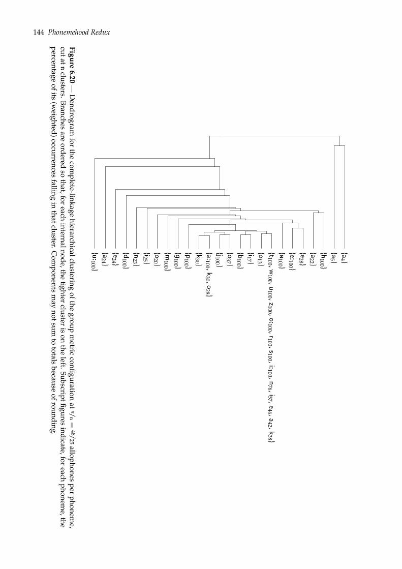
144 Phonemehood Redux
u:100 a
24 e24 d
100 n
23 i25 o
20 m
100 g
100 p
100 k
30 a:100 ,k
30 ,o28
j100 o
37 b
100 i17 o
13 t100 ,w
100 ,u100 ,z100 ,o:100 ,r100 ,s100 ,i:100 ,n
76 ,i57 ,e46 ,a42 ,k
38 ð
100 e:100 e28 a
22 h
100 a
5 a
4
Figure6.20
—Dendrogram
forthecom
plete-linkagehierarchicalclustering
ofthegroup
metric
configurationat
n/n=
48/25allophonesperphonem
e,cutat
nclusters.Branchesare
orderedso
that,foreachinternalnode,the
tighterclusterisonthe
left.Subscriptfiguresindicate,foreachphonem
e,thepercentage
ofits(weighted)occurrencesfalling
inthatcluster.C
omponentsm
aynotsum
tototalsbecause
ofrounding.
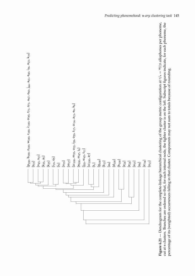
Predicting phonemehood: n-ary clustering task 145
o13
e
: 54
a8
a15
e
24
e24
h
100
d10
0a
9k
13
g10
0t
εu
: 100
,a7
j 55,
e:45
,t11
ð
100,
m47
,i6
a: 1
00,m
35,u
32,i
28,o
20,t
17,o
: 14,
a 13,
e 9,k
6m
17
n33
i 9
i 1
9,o 5
k
25
k35
,a3
n43
,s13
s
15
p10
0,b 1
00,z
100,
w10
0,r 1
00,i
: 100
,o: 8
5,t 7
1,s 7
1,u 6
7,o 6
0,j 4
4,a 4
1,e 4
0,i 3
6,n 2
3,k 1
9
Figu
re6.21
—Den
drog
ram
forthe
complete-lin
kage
hierarch
ical
clus
terin
gof
thegrou
pmetric
confi
guratio
nat
n /n=
98/2
5alloph
ones
perp
hone
me,
cuta
tnclus
ters.B
ranc
hesa
reorde
redso
that,for
each
internal
node
,the
tighter
clus
teriso
ntheleft.
Subscriptfi
guresind
icate,fore
achph
onem
e,the
percen
tage
ofits
(weigh
ted)
occu
rren
cesfallin
gin
that
clus
ter.Com
pone
ntsm
ayno
tsum
tototalsbe
caus
eof
roun
ding
.
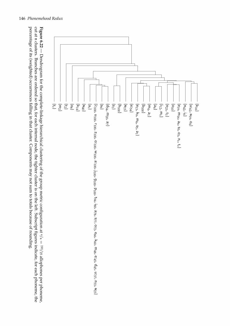
146 Phonemehood Redux
tε
m2
t2 o
8 k
14 ð
40 a
ε i:100 ,u
100 ,r100 ,z100 ,o:100 ,w100 ,a:100 ,j100 ,g
100 ,p100 ,t94 ,i80 ,a
78 ,s77 ,o72 ,e66 ,k
60 ,m48 ,e:45 ,d
45 ,u:37 ,n33 ,ð
23 s9 d
54 ,m20 ,a
7 s1 h
100 ð
15 e:54 e13 ,k
9 ,m6 ,s5 ,a
1 b
100 m
4 ,a1
a4
i12 ,mε
n23 ,t1
o10
e19 ,m16 ,a
6 ,s5 ,o3 ,n
ε ,tε
n42 ,i6
u:62 ,ð19 ,o
4 k
16
Figure6.22
—Dendrogram
forthecom
plete-linkagehierarchicalclustering
ofthegroup
metricconfiguration
atn/
n=
191/25allophonesperphonem
e,cutat
nclusters.Branchesare
orderedso
that,foreachinternalnode,the
tighterclusterisonthe
left.Subscriptfiguresindicate,foreachphonem
e,thepercentage
ofits(weighted)occurrencesfalling
inthatcluster.C
omponentsm
aynotsum
tototalsbecause
ofrounding.
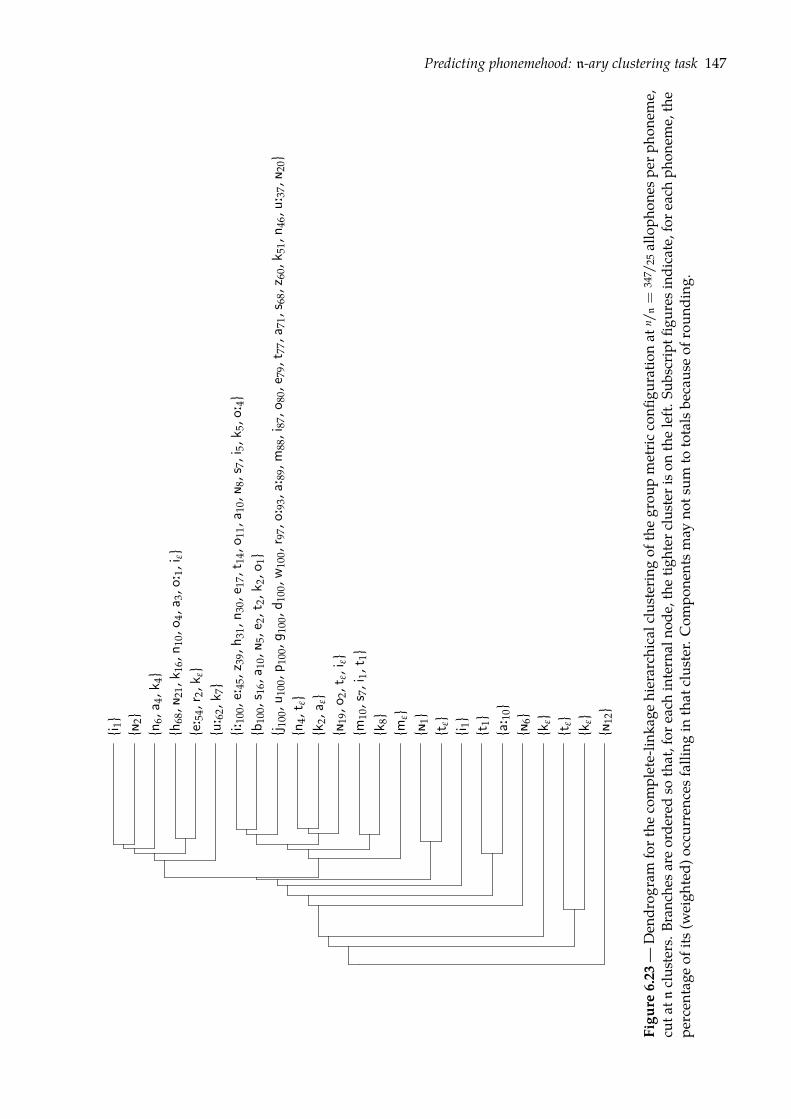
Predicting phonemehood: n-ary clustering task 147
ð12
k
εt
εk
εð
6a
: 10
t1
i 1
tε
ð1
mε
k8
m10
,s7,
i 1,t
1ð
19,o
2,t ε
,iε
k2,
a ε
n4,
t ε
j 100
,u10
0,p 1
00,g
100,
d 100
,w10
0,r 9
7,o:
93,a
: 89,
m88
,i87
,o80
,e79
,t77
,a71
,s68
,z60
,k51
,n46
,u: 3
7,ð 2
0b
100,
s 16,
a 10,
ð 5,e
2,t 2
,k2,
o 1
i:10
0,e:
45,z
39,h
31,n
30,e
17,t
14,o
11,a
10,ð
8,s 7
,i5,
k 5,o
: 4
u: 6
2,k 7
e
: 54,
r 2,k
εh
68,ð
21,k
16,n
10,o
4,a 3
,o: 1
,iε
n6,
a 4,k
4ð
2i 1
Figu
re6.23
—Den
drog
ram
forthe
complete-lin
kage
hierarch
ical
clus
terin
gof
thegrou
pmetric
confi
guratio
nat
n /n=
347 /
25alloph
ones
perp
hone
me,
cuta
tnclus
ters.B
ranc
hesa
reorde
redso
that,for
each
internal
node
,the
tighter
clus
teriso
ntheleft.
Subscriptfi
guresind
icate,fore
achph
onem
e,the
percen
tage
ofits
(weigh
ted)
occu
rren
cesfallin
gin
that
clus
ter.Com
pone
ntsm
ayno
tsum
tototalsbe
caus
eof
roun
ding
.
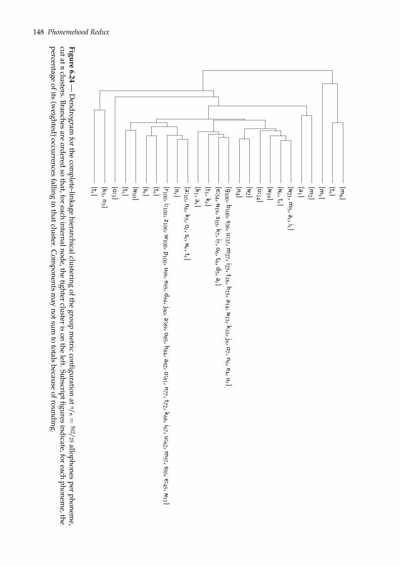
148 Phonemehood Redux
tε
k5 ,n
3 o:3 t
ε ð
10 s
ε t
ε r100 ,i:100 ,z100 ,w
100 ,p100 ,u
99 ,e95 ,d94 ,j90 ,a:89 ,o
85 ,h84 ,a
82 ,o:81 ,n77 ,t72 ,k
68 ,i67 ,u:62 ,m57 ,s50 ,e:45 ,ð
11 n
ε a:10 ,n
6 ,k5 ,o
ε ,sε ,ð
ε ,tε
k1 ,a
ε t1 ,k
ε e:54 ,ð
19 ,s10 ,k7 ,i7 ,o
6 ,t6 ,d5 ,a
ε g
100 ,b100 ,s38 ,u:37 ,m
27 ,i25 ,t18 ,h15 ,a
14 ,ð13 ,k
10 ,j9 ,o7 ,n
6 ,e4 ,uε
n4
ð2
o:14 ð
19 ð
ε ,tε
ð21 ,m
5 ,aε ,iε
a1
m2
mε
tε
m6
Figure6.24
—Dendrogram
forthecom
plete-linkagehierarchicalclustering
ofthegroup
metricconfiguration
atn/
n=
502/25allophonesperphonem
e,cutat
nclusters.Branchesare
orderedso
that,foreachinternalnode,the
tighterclusterisonthe
left.Subscriptfiguresindicate,foreachphonem
e,thepercentage
ofits(weighted)occurrencesfalling
inthatcluster.C
omponentsm
aynotsum
tototalsbecause
ofrounding.
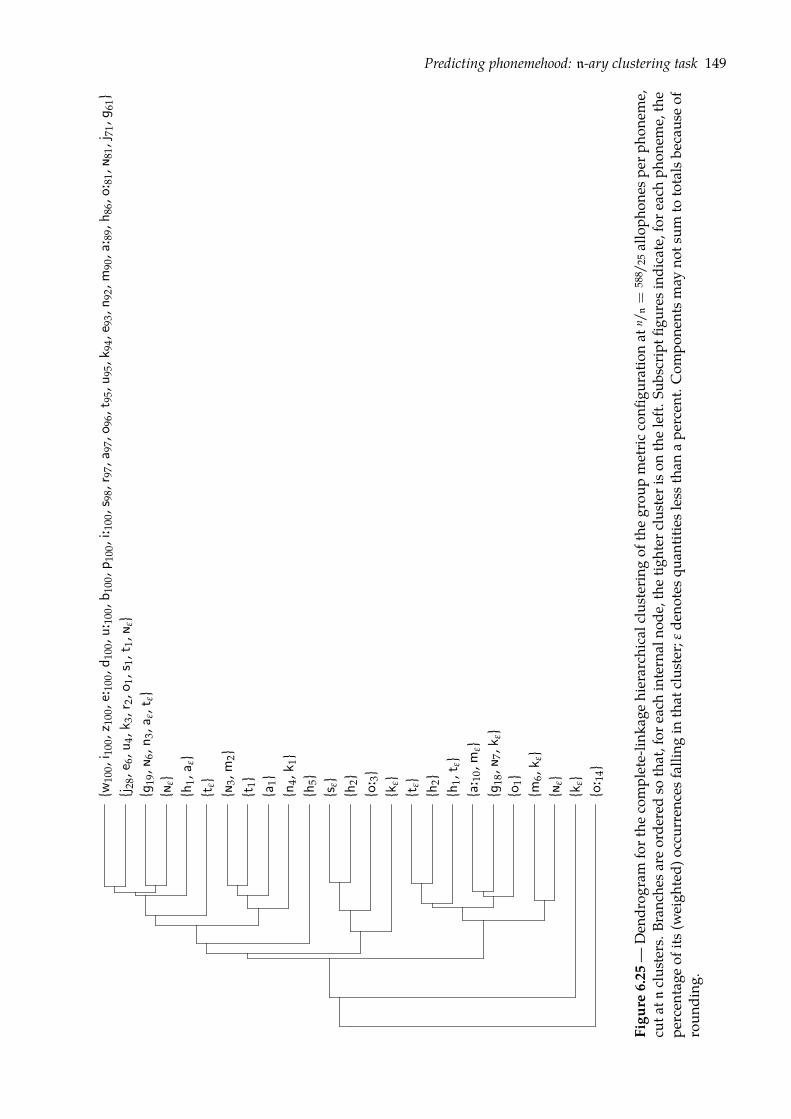
Predicting phonemehood: n-ary clustering task 149
o: 1
4k
εð
εm
6,k ε
o
1g
18,ð
7,k ε
a
: 10,
mε
h1,
t ε
h2
tε
kε
o: 3
h
2s
εh
5n
4,k 1
a
1t
1ð
3,m
2t
εh
1,a ε
ð
εg
19,ð
6,n 3
,aε,
t ε
j 28,
e 6,u
4,k 3
,r2,
o 1,s
1,t 1
,ðε
w10
0,i 1
00,z
100,
e:10
0,d 1
00,u
: 100
,b10
0,p 1
00,i
: 100
,s98
,r97
,a97
,o96
,t95
,u95
,k94
,e93
,n92
,m90
,a: 8
9,h 8
6,o:
81,ð
81,j
71,g
61
Figu
re6.25
—Den
drog
ram
forthe
complete-lin
kage
hierarch
ical
clus
terin
gof
thegrou
pmetric
confi
guratio
nat
n /n=
588 /
25alloph
ones
perp
hone
me,
cuta
tnclus
ters.B
ranc
hesa
reorde
redso
that,for
each
internal
node
,the
tighter
clus
teriso
ntheleft.
Subscriptfi
guresind
icate,fore
achph
onem
e,the
percen
tage
ofits
(weigh
ted)
occu
rren
cesfallin
gin
that
clus
ter;
εde
notesq
uantities
less
than
ape
rcen
t.Com
pone
ntsm
ayno
tsum
tototalsbe
caus
eof
roun
ding
.

150 Phonemehood Redux
6.6 Overall assessment
In this chapter, we presented the major contribution of the present study, i.e. a complete refor-mulation of Peperkamp et al.’s (2006) framework based on three-way MDS. Given three-wayinput dissimilarities, MDS models yield metric configurations in Euclidean spaces of arbitrarydimensionality, so that the point-to-point distances in that space account for the input phone-to-phone dissimilarities. We further showed in Section 6.4 that such Euclidean embeddings of ourindicators of allophony do not smear the information contained in the indicators.
The main conclusions of this chapter, however, that indicators of allophony are not indicatorsof phonemehood—as uniformly showed by the various prognosis, classification, and clusteringresults presented in Sections 6.2, 6.3, 6.4, and 6.5. Although such results are, at a first glance,disappointing, we argued in Section 6.5.1 that the odds of randomly discovering the referencephonemic partition P are virtually null.
Further research is thus needed in order to develop indicators that are not only stronglycorrelated with allophony, but also with phonemehood, i.e. with the identity of phonemes.
CHAPTER 7CONCLUSION
The pervasiveness of allophonic processes in natural languages is undeniable. In light of priorscholarship and of the experiments presented throughout this dissertation, the question of howinfants may acquire the phonemic inventory of their native language remains an open question.The general conclusion of our work is indeed that no acoustic, temporal, distributional, or lexicalindicator of allophony (or any combination thereof) appears to contain enough information forthe discovery of well-separated, phoneme-like sound categories.
In this final chapter, we review the scientific question motivating the present study, as well asour contribution to knowledge. We then go on to discuss recommendations for future research,notably in view of the various linguistic and computational limitations of our work.
7.1 Indicators of allophony and phonemehood
This dissertation describes a modeling project aimed at assessing the relevance and effectivenessof various linguistic cues, in the interest of reducing the considerable, inherent variabilityin speech to a small number of sounds categories, i.e. the phonemes of the target language.Throughout the present study, we assumed the position of a naive learner—more precisely,that of an infant acquiring its native language. Indeed, having observed that the realizationsof a given phoneme are constrained by the surrounding phonemes (or the realizations thereof,cf. Figure 2.2), one can but be puzzled by the apparent ease with which infants bootstrap intolanguage. How, for instance, do Japanese-learning infants discover that the third sounds in[miso] ∼ [moSi] (miso ∼ moshi) are both to be processed as realizations of the same abstract soundcategory? What kind of cues may English-learning infants rely on to learn that [sINkIN] ∼ [TINkIN](sinking ∼ thinking) can not refer to the same action?
The work presented in this dissertation builds upon the line of computational studies initiatedby Peperkamp et al. (2006). The common hypothesis underlying this body of work is that infantsare able to keep track of—and rely on—phone-to-phone dissimilarity judgments in order toeventually cluster similar phones into phonemic categories. In Chapter 4, we showed that allpreviously proposed phone-to-phone dissimilarities can actually be reformulated as variousinstances of a single, cohesive concept, viz. indicators of allophony. In that chapter, we thenbenchmarked the (relative) efficiency of indicators of allophony that rely on different typesof linguistic cues, i.e. measures of near-complementary distributions (Peperkamp et al., 2006;Le Calvez et al., 2007), acoustic similarity (Dautriche, 2009), lexical dissimilarity (Martin et al.,2009; Boruta, 2011b), and temporal similarity—a novel class of indicators introduced in this study.To this aim, we amended Peperkamp et al.’s (2006) artificial learner in order to obtain empiricalupper bounds on the learnability of the allophony relation, i.e. the binary relation that bringstogether phones that are realizations of the same phoneme. Throughout the extensive evaluationcarried out in Chapter 4, we showed that indicators’ effectiveness at distinguishing between
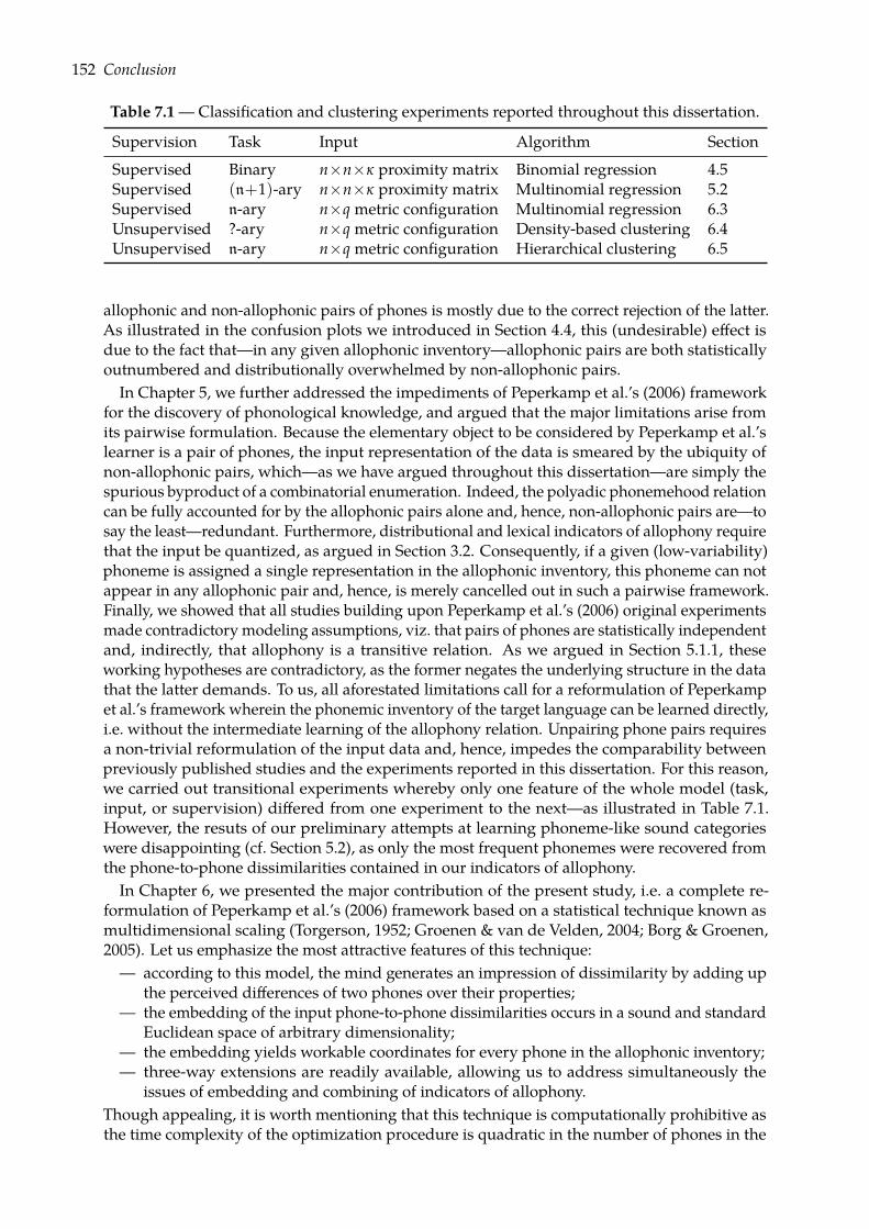
152 Conclusion
Table 7.1 —Classification and clustering experiments reported throughout this dissertation.
Supervision Task Input Algorithm Section
Supervised Binary n×n×κ proximity matrix Binomial regression 4.5Supervised (n+1)-ary n×n×κ proximity matrix Multinomial regression 5.2Supervised n-ary n×q metric configuration Multinomial regression 6.3Unsupervised ?-ary n×q metric configuration Density-based clustering 6.4Unsupervised n-ary n×q metric configuration Hierarchical clustering 6.5
allophonic and non-allophonic pairs of phones is mostly due to the correct rejection of the latter.As illustrated in the confusion plots we introduced in Section 4.4, this (undesirable) effect isdue to the fact that—in any given allophonic inventory—allophonic pairs are both statisticallyoutnumbered and distributionally overwhelmed by non-allophonic pairs.In Chapter 5, we further addressed the impediments of Peperkamp et al.’s (2006) framework
for the discovery of phonological knowledge, and argued that the major limitations arise fromits pairwise formulation. Because the elementary object to be considered by Peperkamp et al.’slearner is a pair of phones, the input representation of the data is smeared by the ubiquity ofnon-allophonic pairs, which—as we have argued throughout this dissertation—are simply thespurious byproduct of a combinatorial enumeration. Indeed, the polyadic phonemehood relationcan be fully accounted for by the allophonic pairs alone and, hence, non-allophonic pairs are—tosay the least—redundant. Furthermore, distributional and lexical indicators of allophony requirethat the input be quantized, as argued in Section 3.2. Consequently, if a given (low-variability)phoneme is assigned a single representation in the allophonic inventory, this phoneme can notappear in any allophonic pair and, hence, is merely cancelled out in such a pairwise framework.Finally, we showed that all studies building upon Peperkamp et al.’s (2006) original experimentsmade contradictory modeling assumptions, viz. that pairs of phones are statistically independentand, indirectly, that allophony is a transitive relation. As we argued in Section 5.1.1, theseworking hypotheses are contradictory, as the former negates the underlying structure in the datathat the latter demands. To us, all aforestated limitations call for a reformulation of Peperkampet al.’s framework wherein the phonemic inventory of the target language can be learned directly,i.e. without the intermediate learning of the allophony relation. Unpairing phone pairs requiresa non-trivial reformulation of the input data and, hence, impedes the comparability betweenpreviously published studies and the experiments reported in this dissertation. For this reason,we carried out transitional experiments whereby only one feature of the whole model (task,input, or supervision) differed from one experiment to the next—as illustrated in Table 7.1.However, the resuts of our preliminary attempts at learning phoneme-like sound categorieswere disappointing (cf. Section 5.2), as only the most frequent phonemes were recovered fromthe phone-to-phone dissimilarities contained in our indicators of allophony.In Chapter 6, we presented the major contribution of the present study, i.e. a complete re-
formulation of Peperkamp et al.’s (2006) framework based on a statistical technique known asmultidimensional scaling (Torgerson, 1952; Groenen & van de Velden, 2004; Borg & Groenen,2005). Let us emphasize the most attractive features of this technique:— according to this model, the mind generates an impression of dissimilarity by adding up
the perceived differences of two phones over their properties;— the embedding of the input phone-to-phone dissimilarities occurs in a sound and standard
Euclidean space of arbitrary dimensionality;— the embedding yields workable coordinates for every phone in the allophonic inventory;— three-way extensions are readily available, allowing us to address simultaneously the
issues of embedding and combining of indicators of allophony.Though appealing, it is worth mentioning that this technique is computationally prohibitive asthe time complexity of the optimization procedure is quadratic in the number of phones in the
Future research 153
allophonic inventory—to say nothing of the number of iterations, dimensions, and combinedindicators. Be that as it may, we consider multidimensional scaling an effective technique, chieflyon the grounds that it allows for the use of individual phones as the elementary objects to beconsidered by the learner. Relying on such Euclidean embeddings of indicators of allophony (andcombinations thereof), we further argued in Chapter 6 that the task of learning the phonemicinventory of the target language can in fact be recast as a standard partitioning-clustering task,whereby the learner has to partition a set of phones into collectively exhaustive and mutuallyexclusive phonemes. We then carried out various classification and clustering experimentswhose results consistently indicate that effective indicators of allophony are not necessarilyeffective indicators of phonemehood. Indeed, none of the indicators of allophony we consideredin the present study appears to provide compact or well-separated phoneme-like clusters. Inother words, our input data violate the compactness hypothesis that underlies most clusteringproblems (Duin, 1999; Pękalska et al., 2003) and, as we argued in Section 2.1, early languageacquisition. Although attempting to learn the phonemehood relation from such data thusappears to be in vain, it is worth highlighting our explanation in Section 6.4 that the mediocreperformance we observed throughout Chapter 6 is not the consequence of our embedding-basedreformulation of the problem: using the original phone-to-phone dissimilarities does not yieldmodels with a better predictive power in the interest of discovering phonemes.Altogether, the computational results we discussed throughout this dissertation suggest that
allophony and phonemehood can only be discovered from acoustic, temporal, distributional, orlexical indicators at low allophonic complexities, i.e. when—on average—phonemes do not havemany allophones in the quantized representation of the input. Two competing explanationsmay account for this fact. Were infants to tackle a considerable number of allophones, the workreported in this dissertation would fail to propose a plausible account of early phonologicalacquisition. On the contrary, were infants to tackle a number of allophones commensurable withthe allophonic complexities at which our models were evaluated, then the point at which theperformance of our models suffer a significant drop would be interpreted as an assessment ofthe number of allophonic processes at stake in infant-directed speech.
7.2 Future research
A number of issues and limitations have been brought to light during this work. First, becauseof the limited availability of databases of infant-directed speech with aligned transcriptions, wehave used a corpus of adult-directed speech, viz. the Corpus of Spontaneous Japanese (Maekawaet al., 2000; Maekawa, 2003). However, as we argued in Section 3.1, using infants’ linguistic inputto model infants’ linguistic behavior would be a more plausible alternative. Furthermore, weconsider that computational models of early language acquisition should be evaluated usingdata from typologically different languages in order to assess their sensitivity to linguisticdiversity (Gambell & Yang, 2004; Boruta et al., 2011). We therefore leave as a recommendation forfuture research the task of reproducing the work presented throughout this dissertation usingother corpora in order to assess whether our conclusions can be applied generally to languageacquisition, or if they are mere numerical accidents due to the serendipitous, conjoint use of thisparticular corpus of Japanese and, for example, density-based clustering.
Moreover, we have shown in the present study that acoustic, temporal, distributional, orlexical indicators of allophony yield dissimilarity judgments whereby non-allophonic pairsof phones tend to be more dissimilar that allophonic pairs—hence confirming the relevanceof Peperkamp et al.’s (2006) proposal. We have also shown that such indicators are, however,perfectible, as they do not yield an acceptable separation of the phonemes of the target language.Further research is thus needed to fully transform indicators of allophony into indicators ofphonemehood. Regarding the particular framework upon which our work builds, anotheradvancement would consist in examining the relative influence of the constraints one can put onthe three-way multidimensional scaling models. In the absence of a priori linguistic knowledge—
154 Conclusion
as well as prior scholarship on the use of such models for language-related problems—we indeedfavored the least constrained three-way model. Though non-trivial, we acknowledge that thischoice was arbitrary and, thus, that its consequences need to be further investigated.
Finally, let us revisit a fundamental assumption of the work presented in this dissertation: thedevelopment of speech perception is an innately guided learning process (Jusczyk & Bertoncini,1988; Gildea & Jurafsky, 1996; Plunkett, 1997; Bloom, 2010). Our results confirm this assumptionin the sense that density-based clustering, i.e. the least constrained of all algorithms we used,yielded the least accurate predictions. The crucial point here is that the discovery of linguis-tic knowledge is facilitated—if not simply made possible—by a priori linguistic constraints.Interestingly enough, Johnson et al. (2007) recently proposed a class of probabilistic modelsof language, referred to as adaptor grammars, that can be constrained so as to account forsome given linguistic structure. This approach has been used to develop and validate variouscomputational models of the acquisition of word segmentation (Johnson, 2008a,b) but, to ourknowledge, no experiment focusing on the acquisition of phonological categories has yet beenreported. We therefore leave as a recommendation for future research the task of assessingwhether providing an artificial learner with computational constraints or linguistic structurefacilitates the acquisition of phonemes, as, in the words of Bloom (2010):
One lesson from the study of artificial intelligence [...] is that an empty head learns nothing:a system that is capable of rapidly absorbing information needs to have some prewiredunderstanding of what to pay attention to and what generalizations to make. Babies mightstart off smart, then, because it enables them to get smarter.~

Shadow didn’t wait to see. He walked away and he kept on walking.~—Neil Gaiman, in American Gods

REFERENCES
Nota bene Numbers in square brackets are backreferences to the main text.
Abney, S. (2011). Data-intensive experimental linguistics. Linguistic Issues in Language Technol-ogy 6(2). [pp. 20 and 22]
Agresti, A. (2007). An Introduction to Categorical Data Analysis (second ed.). Hoboken, New Jersey:John Wiley & Sons, Inc. [pp. 23, 83, 84, 85, 88, 102, 103, and 127]
Akaike, H. (1974). A new look at the statistical model identification. IEEE Transactions onAutomatic Control 19(6), 716–723. [p. 86]
Aliguliyev, R.M. (2009). Performance evaluation of density-based clusteringmethods. InformationSciences 179, 3583–3602. [pp. 100 and 125]
Alishahi, A. (2011). Computational Modeling of Human Language Acquisition. Synthesis Lectureson Human Language Technologies. Morgan & Claypool. [pp. 21, 23, and 82]
AMLaP. Architectures and mechanisms for language processing. http://www.amlap.org/.[p. 22]
Ankerst, M., M. M. Breunig, H.-P. Kriegel, and J. Sander (1999). OPTICS: ordering points toidentify the clustering structure. In Proceedings of the ACM SIGMOD International Conference onManagement of data, pp. 49–60. ACM Press. [p. 135]
Aslin, R. N., J. R. Saffran, and E. L. Newport (1998). Computation of conditional probabilitystatistics by 8-month old infants. Psychological Science 9, 321–324. [pp. 19 and 24]
Atkinson, Q. D. (2011). Phonemic diversity supports a serial founder effect model of languageexpansion from Africa. Science 332(6027), 346–349. [pp. 14 and 157]
Austin, W. M. (1957). Criteria for phonetic similarity. Language 33(4), 538–544. [pp. 15 and 54]Bane, M. (2011). simplegoodturing: a Python module implementing the “Simple Good–Turing”method of frequency estimation described by Gale & Sampson (1995), version 0.3. RetrievedOctober 21, 2011. https://github.com/maxbane/simplegoodturing. [p. 60]
Barzily, Z., Z. Volkovich, B. Akteke-Öztürk, and G.-W. Weber (2009). On a minimal spanningtree approach in the cluster validation problem. Informatica 20(2), 187–202. [p. 125]
Berdicevskis, A. andA. C. Piperski (2011). Doubts about a serial founder-effect model of languageexpansion. Science. Response to Atkinson’s (2011) article. Published online 8 December 2011.http://www.sciencemag.org/content/332/6027/346.abstract/reply. [p. 22]
Bergstra, J. and Y. Bengio (2012). Random search for hyper-parameter optimization. Journal ofMachine Learning Research 13, 281–305. [pp. 134 and 135]
Bezdek, J. C. and N. R. Pal (1998). Some new indices of cluster validity. IEEE Transactions onSystems, Man and Cybernetics 28(3), 301–315. [pp. 100 and 125]
Bhattacharyya, A. (1943). On ameasure of divergence between two statistical populations definedby their probability distributions. Bulletin of the Calcutta Mathematical Society 35, 99–109. [p. 59]
158 References
Bloom, P. (2010). The moral life of babies. The New York Times Magazine, MM44. May 9, 2010.[pp. 19, 24, and 154]
Boersma, P. (2010). Modelling phonological category learning. Accessed March 15, 2012.http://www.fon.hum.uva.nl/paul/. [pp. 21 and 24]
Boersma, P. (2011). A programme for bidirectional phonology and phonetics and their acquisitionand evolution. In A. Benz and J. Mattausch (eds.), Bidirectional Optimality Theory, pp. 33–72.Amsterdam: John Benjamins. [p. 21]
Boersma, P., P. Escudero, and R. Hayes (2003). Learning abstract phonological from auditoryphonetic categories: an integrated model for the acquisition of language-specific sound cate-gories. In Proceedings of the Fifteenth International Congress of Phonetic Sciences, Barcelona, pp.1013–1016. [p. 21]
Boersma, P. and C. Levelt (2000). Gradual constraint-ranking learning algorithm predicts acqui-sition order. In Proceedings of Thirtieth Child Language Research Forum, Stanford, California, pp.229–237. [p. 21]
Boersma, P. and C. Levelt (2003). Optimality theory and phonological acquisition. Volume 3, pp.1–50. [p. 21]
Borg, I. and P. J. F. Groenen (2005). Modern Multidimensional Scaling: Theory and Applications(second ed.). Springer Series in Statistics. [pp. 116, 117, 118, 119, 120, 121, and 152]
Boruta, L. (2009). Acquisition précoce des règles allophoniques: approche computationnelle.Master’s thesis, Université Paris Diderot. [pp. 21, 22, 26, 33, 34, 51, 61, 62, 66, 75, 82, 94, 95, 98,and 106]
Boruta, L. (2011a). A note on the generation of allophonic rules. Technical Report #0401, INRIA.[pp. 26, 33, 34, and 35]
Boruta, L. (2011b). Combining indicators of allophony. In Proceedings of the ACL 2011 StudentSession, Portland, Oregon, pp. 88–93. Association for Computational Linguistics. [pp. 16, 21,22, 26, 33, 34, 51, 53, 59, 61, 62, 63, 64, 66, 69, 74, 75, 76, 82, 87, 88, 95, 98, 106, and 151]
Boruta, L., S. Peperkamp, B. Crabbé, and E. Dupoux (2011). Testing the robustness of onlineword segmentation: effects of linguistic diversity and phonetic variation. In Proceedings of the2nd Workshop on Cognitive Modeling and Computational Linguistics, Portland, Oregon, pp. 1–9.Association for Computational Linguistics. [pp. 20, 21, 26, 33, 34, 62, and 153]
Brannen, K. (2002). The role of perception in differential substitution. The Canadian Journal ofLinguistics 47(1/2), 1–46. [p. 14]
Brent, M. R. (1999). An efficient, probabilistically sound algorithm for segmentation and worddiscovery. Machine Learning 34(1–3), 71–105. [pp. 20, 21, 61, 82, and 166]
Brent, M. R. and T. A. Cartwright (1996). Distributional regularity and phonotactic constraintsare useful for segmentation. Cognition 61, 93–125. [pp. 20 and 61]
Bronstein, M. M., A. M. Bronstein, R. Kimmel, and I. Yavneh (2005). A multigrid approach formulti-dimensional scaling. In Proceedings of the Twelfth Copper Mountain Conference on MultigridMethods. [p. 117]
Carroll, J. D. and J.-J. Chang (1970). Analysis of individual differences in multidimensionalscaling via an n-way generalization of “Eckart-Young” decomposition. Psychometrika 35(2),283–319. [p. 119]
Chen, X., P. Ender, M. Mitchell, and C. Wells (2012). Logistic regression with Stata. UCLA:Academic Technology Services, Statistical Consulting Group. Accessed April 15, 2012.http://www.ats.ucla.edu/stat/stata/webbooks/logistic/. [pp. 83, 84, and 85]
Chomsky, N. and M. Halle (1968). The Sound Pattern of English (1991 ed.). The MIT Press. [pp. 14,16, 21, 35, and 45]
Chou, C.-H., M.-C. Su, and E. Lai (2004). A new cluster validity measure and its application to
References 159
image compression. Pattern Analysis and Applications 7, 205–220. [p. 125]Christiansen, M. H., J. Allen, and M. Seidenberg (1998). Learning to segment speech usingmultiple cues. Language and Cognitive Processes 13(2), 221–268. [pp. 20 and 61]
Clapper, B. M. (2009). munkres: a Python module implementing the “Hungarian method”described by Munkres (1957). Version 1.0.5.3. http://software.clapper.org/munkres/. [p. 56]
Clark, E. V. (2004). How language acquisition builds on cognitive development. Trends in CognitiveSciences 8(10), 472–478. [p. 18]
CMCL. Cognitive modeling and computational linguistics. http://www.psy.cmu.edu/~cmcl/.[p. 22]
Coleman, J. (1998). Phonological representations: their names, forms, and powers. Cambridge Studiesin Linguistics 85. Cambridge: Cambridge University Press. [pp. 13, 14, and 24]
Coolen, A. C. C., R. Kühn, and P. Sollich (2005). Theory of Neural Information Processing Systems.Oxford: Oxford University Press. [p. 63]
Cormen, T. H., C. E. Leiserson, R. L. Rivest, and C. Stein (2001). Introduction to Algorithms (seconded.). The MIT Press. [pp. 56 and 98]
Cover, T. M. and J. A. Thomas (2006). Elements of Information Theory (second ed.). Wiley–Interscience. [p. 59]
Cristia, A. (2011). Ongoing meta-analysis on the acoustics of infant-directed speech. AccessedSeptember 15, 2011. https://sites.google.com/site/acrsta/ids_meta-analysis. [p. 26]
CSJ DVD (2004). The Corpus of Spontaneous Japanese, offline documentation. A collection of 17 PDFfiles in Japanese, bundled in the /DOC directory of the DVD “Volume 1”. [pp. 26, 27, 28, 29, 30,41, and 47]
CSJ Website (2012). The Corpus of Spontaneous Japanese, online documentation. Accessed January 15,2012. http://www.ninjal.ac.jp/products-k/katsudo/seika/corpus/public/. [pp. 25 and 27]
Daland, R. and J. B. Pierrehumbert (2011). Learning diphone-based segmentation. CognitiveScience 35(1), 119–155. [pp. 20 and 26]
Dautriche, I. (2009). Modélisation des processus d’acquisition du langage par des méthodesstatistiques. Master’s thesis, Institut National des Sciences Appliquées, Toulouse. [pp. 21, 22,26, 27, 28, 33, 34, 35, 36, 37, 38, 51, 54, 55, 56, 61, 64, 74, 75, 82, 94, 95, 98, 106, and 151]
de Leeuw, J. (1988). Convergence of the majorization method for multidimensional scaling.Journal of Classification 5, 163–180. [p. 117]
de Leeuw, J. and P. Mair (2009). Multidimensional scaling using majorization: SMACOF in R.Journal of Statistical Software 31(3), 1–30. Version 1.0-0. [pp. 116, 117, 118, 119, and 120]
Dell, F. (1985). Les règles et les sons, introduction à la phonologie générative (second ed.). CollectionSavoir. Paris: Hermann. [p. 14]
Dillon, B., E. Dunbar, and W. Idsardi (2012). A single stage approach to learning phonologicalcategories: insights from Inuktitut. Cognitive Science. To appear. [p. 22]
Dudoit, S. and J. Fridlyand (2002). A prediction-based resampling method for estimating thenumber of clusters in a dataset. Genome Biology 3(7), 1–21. [p. 125]
Duin, R. P.W. (1999). Compactness and complexity of pattern recognition problems. In C. Perneel(ed.), Proceedings of the International Symposium on Pattern Recognition “In Memoriam PierreDevijver", Brussels, pp. 124–128. [pp. 16, 53, 116, 125, and 153]
Duin, R. P. W. and E. Pękalska (2012). The dissimilarity space: bridging structural and statisticalpattern recognition. Pattern Recognition Letters 33, 826–832. [p. 121]
Dunbar, E. (2009). Pitfalls of distributional allophone learning. Presentation given at theMontreal-Ottawa-Toronto Phonology Workshop. [p. 59]
Dunn, J. C. (1973). A fuzzy relative of the ISODATAprocess and its use in detectingwell-separated
160 References
clusters. Journal of Cybernetics 3(3), 32–57. [p. 125]Eifring, H. B. and R. Theil (2004). Linguistics for Students of Asian and African Languages. Instituttfor østeuropeiske og orientalske studier. [p. 13]
Ellis, N. C. (2002). Frequency effects in language processing: a review with implications fortheories of implicit and explicit language acquisition. Studies in Second Language Acquisition 24,143–188. [p. 19]
Elman, J. L. (1990). Finding structure in time. Cognitive Sciences 14, 179–211. [pp. 20 and 61]Elsner, M., S. Goldwater, and J. Eisenstein (2012). Bootstrapping a unified model of lexicaland phonetic acquisition. In Proceedings of the Fiftieth Annual Meeting of the Association ofComputational Linguistics, Jeju Island. [p. 20]
Esmaelnejad, J., J. Habibi, and S. H. Yeganeh (2010). A novel method to find appropriate for ε forDBSCAN. In N. T. Nguyen, M. T. Le, and J. Świątek (eds.), Proceedings of the Second InternationalConference on Intelligent Information and Database Systems: Part I, Berlin, Heidelberg, pp. 93–102.Springer-Verlag. [pp. 134 and 135]
Esposito, F., D. Malerba, V. Tamma, and H.-H. Bock (2000). Classical resemblance measures.In H.-H. Bock and E. Diday (eds.), Analysis of Symbolic Data. Exploratory methods for extractingstatistical information from complex data., Chapter 8. Heidelberg: Springer Verlag. [p. 64]
Ester, M., H.-P. Kriegel, J. Sander, and X. Xu (1996). A density-based algorithm for discoveringclusters in large spatial databases with noise. In Proceedings of the Second International Conferenceon Knowledge Discovery and Data Mining, Portland, Oregon. [pp. 133, 134, and 135]
Everson, L. R. H. and W. T. Penzhorn (1988). Experimental comparison on several distancemeasures for speech processing applications. In Proceedings of the Southern African Conferenceon Communications and Signal Processing, pp. 12–17. [p. 54]
Faraway, J. J. (2005). Linear Models with R. Boca Raton, Florida: Chapman & Hall / CRC. [pp. 83and 86]
Faraway, J. J. (2006). Extending the Linear Model with R: Generalized Linear, Mixed Effects andNonparametric Regression Models. Boca Raton, Florida: Chapman & Hall / CRC. [pp. 83, 85,102, and 103]
Farnetani, E. (1997). Coarticulation and connected speech processes. In W. J. Hardcastle andJ. Laver (eds.), The Handbook of Phonetic Sciences, Chapter 12, pp. 371–404. Blackwell Publishers.[p. 16]
Ferrer-i-Cancho, R. and R. V. Solé (2001). Two regimes in the frequency of words and the originsof complex lexicons: Zipf’s law revisited. Journal of Quantitative Linguistics 8(3), 165–173. [p. 32]
Ferrer-i-Cancho, R. and R. V. Solé (2003). Least effort and the origins of scaling in human language.Proceedings of the National Academy of Sciences of the United States of America (PNAS) 100(3), 788–791. [p. 32]
Floyd, R. W. (1962). Algorithm 97: shortest path. Communications of the ACM 5(6). [p. 98]Forgy, E. W. (1965). Cluster analysis of multivariate data: efficiency vs. interpretability ofclassifications. Biometrics 21, 768–769. [p. 142]
Gale, W. A. and K. Church (1994). What’s wrong with adding one? In N. Oostdijk and P. de Haan(eds.), Corpus-Based Research into Language: In honour of Jan Aarts, Amsterdam, pp. 189–200.[p. 60]
Gale, W. A. and G. Sampson (1995). Good–turing frequency estimation without tears. Journal ofQuantitative Linguistics 2, 217–237. [pp. 60 and 157]
Gambell, T. and C. Yang (2004). Statistics learning and universal grammar: modeling wordsegmentation. In Proceedings of the Twentieth International Conference on Computational Linguistics,pp. 49–52. [pp. 20, 26, and 153]
Gelman, A. and J. Hill (2007). Data analysis using regression and multilevel/hierarchical models.
References 161
Analytical methods for social research. New York: Cambridge University Press. [p. 103]Gildea, D. and D. Jurafsky (1996). Learning bias and phonological-rule induction. ComputationalLinguistics 22, 497–530. [pp. 19, 21, 24, and 154]
Giorgino, T. (2009). Computing and visualizing dynamic time warping alignments in R: the dtwpackage. Journal of Statistical Software 31(7), 1–24. [p. 54]
Godfrey, P., R. Shipley, and J. Gryz (2007). Algorithms and analyses for maximal vector compu-tation. The International Journal on Very Large Data Bases 16(1), 5–28. [p. 76]
Goldberger, J. and H. Aronowitz (2005). A distance measure between GMMs based on theunscented transform and its application to speaker recognition. In Proceedings of the 9thEuropean Conference on Speech Communication and Technology, pp. 1985–1989. [pp. 37, 55, and 56]
Goldsmith, J. and A. Xanthos (2009). Learning phonological categories. Language 85(1), 4–38.[pp. 21 and 24]
Goldsmith, J. A., J. Riggle, and A. C. L. Yu (eds.) (2011). The Handbook of Phonological Theory(second ed.). Wiley–Blackwell. [p. 14]
Goldwater, S., T. L. Griffiths, and M. Johnson (2009). A Bayesian framework for word segmenta-tion: exploring the effects of context. Cognition 112(1), 21–54. [pp. 20 and 61]
Gorawski, M. and R. Malczok (2006a). Towards automatic ε calculation in density-based cluster-ing. In Y. Manolopoulos, J. Pokorný, and T. Sellis (eds.), Advances in Databases and InformationSystems, Volume 4152 of Lecture Notes in Computer Science, pp. 313–328. Berlin, Heidelberg:Springer. [p. 135]
Gorawski, M. andR.Malczok (2006b). AEC algorithm: a heuristic approach to calculating density-based clustering ε parameter. In T. Yakhno and E. Neuhold (eds.), Advances in InformationSystems, Volume 4243 of Lecture Notes in Computer Science, pp. 90–99. Berlin, Heidelberg:Springer. [p. 135]
Goutte, C. and E. Gaussier (2005). A probabilistic interpretation of precision, recall and F-score,with implication for evaluation. In Proceedings of the 27th European Conference on InformationRetrieval, pp. 345–359. [p. 87]
Graham, R. L., D. E. Knuth, and O. Patashnik (1988). Concrete Mathematics. Reading, Mas-sachusetts: Addison–Wesley. Sixth printing, with corrections. [pp. 141 and 142]
Gray, A. and J. Markel (1976). Distance measures for speech processing. IEEE Transactions onAcoustics, Speech, and Signal Processing 24(5). [p. 54]
Groenen, P. J. F. and W. J. Heiser (1996). The tunneling method for global optimization inmultidimensional scaling. Psychometrika 61(3), 529–550. [p. 120]
Groenen, P. J. F. and W. J. Heiser (2000). “Optimization transfer using surrogate objectivefunctions:” discussion. Journal of Computational and Graphical Statistics 9(1), 44–48. [p. 117]
Groenen, P. J. F. and M. van de Velden (2004). Multidimensional scaling. Technical Report EI2004-15, Econometric Institute, Erasmus University Rotterdam. [pp. 116, 120, and 152]
Grønnum, N. and H. Basbøll (2003). Two-phased stød vowels—a cognitive reality? Phonum 9,33–36. Umeå University, Department of Philosophy and Linguistics. [p. 56]
Ha, L. Q., E. I. Sicilia-Garcia, J. Ming, and F. J. Smith (2002). Extension of Zipf’s law to words andphrases. In Proceedings of the Nineteenth International Conference on Computational Linguistics, pp.315–320. [p. 32]
Halkidi, M., Y. Batistakis, and M. Vazirgiannis (2001). On clustering validation techniques.Intelligent Information Systems Journal 17(2–3), 107–145. [p. 125]
Halkidi, M. and M. Vazirgiannis (2001). Clustering validity assessment: finding the optimalpartitioning of a data set. In Proceedings of the IEEE International Conference on Data Mining, pp.187–194. [p. 125]
Harris, Z. S. (1951). Methods in Structural Linguistics. Chicago: University of Chicago Press.
162 References
[pp. 21 and 58]Harris, Z. S. (1955). From phoneme to morpheme. Language 31, 192–222. [p. 21]Hartigan, J. A. and M. A. Wong (1979). A K-means clustering algorithm. Applied Statistics 28,100–108. [p. 142]
Hayes, B. (2004). Phonological acquisition in optimality theory: the early stages. In R. Kager, J. Pa-ter, andW. Zonneveld (eds.), Fixing Priorities: Constraints in Phonological Acquisition. Cambridge:Cambridge University Press. [p. 21]
Hermansky, H. (1999). Mel cepstrum, deltas, double-deltas, ... what else is new? In Proceedingsof the Workshop on Robust Methods for Speech Recognition in Adverse Conditions, Tampere. [p. 35]
Herrnstein, R. J., D. H. Loveland, and C. Cable (1976). Natural concepts in pigeons. Journal ofExperimental Psychology: Animal Behavior Processes 2(4), 285–302. Inaccessible, cited by Martinet al. (2009). [pp. 68, 69, 101, and 106]
Hershey, J. R. and P. A. Olsen (2007). Approximating the Kullback–Leibler divergence betweenGaussian mixture models. In Proceedings of the IEEE International Conference on Acoustics, Speechand Signal Processing, Volume 4, pp. 317–320. [p. 55]
Hinds, J. (1990). Japanese. Croom Helm descriptive grammars. Croom Helm. [pp. 28, 29, 31,and 41]
Hockett, C. (1955). A manual of phonology. International Journal of American Linguistics 21(4).[p. 63]
Hodges, A. (2007). One to Nine: the Inner Life of Numbers. New York & London: W. W. Norton &Company. [p. 23]
Horan, C. B. (1969). Multidimensional scaling: Combining observations when individuals havedifferent perceptual structures. Psychometrika 34, 139–65. [pp. 118 and 119]
Hsu, C.-W., C.-C. Chang, and C.-J. Lin (2010). A practical guide to support vector classification.Technical report, National Taiwan University. [p. 135]
Hubert, L. J. and P. Arabie (1985). Comparing partitions. Journal of Classification 2, 193–218.[p. 125]
Hubert, L. J., P. Arabie, and J. Meulman (2001). Combinatorial data analysis: optimization by dynamicprogramming. Philadelphia: SIAM. [p. 141]
Huijbregts, M., M. McLaren, and D. van Leeuwen (2011). Unsupervised acoustic sub-word unitdetection for query-by-example spoken term detection. In Proceedings of the IEEE InternationalConference on Acoustics, Speech and Signal Processing, pp. 4436–4439. [p. 20]
Hájek, A. (2012). Interpretations of probability. In E. N. Zalta (ed.), The Stanford Encyclopedia ofPhilosophy (Summer 2012 ed.). [p. 19]
Höppner, F. (2009). How much true structure has been discovered? In P. Perner (ed.),MachineLearning and Data Mining in Pattern Recognition, Volume 5632 of Lecture Notes in ComputerScience, pp. 385–397. Springer Berlin / Heidelberg. [pp. 125 and 132]
International Phonetic Association (1999). Phonetic description and the IPA chart. In Handbookof the International Phonetic Association: a guide to the use of the international phonetic alphabet.Cambridge University Press. [pp. 14 and 32]
Ito, J. andA.Mester (1995). Japanese phonology. In J. Goldsmith (ed.), TheHandbook of PhonologicalTheory, pp. 817–838. Blackwell. [pp. 28, 31, 41, and 45]
Jain, A. K. (2008). Data clustering: 50 years beyond k-means. In Proceedings of the 2008 EuropeanConference on Machine Learning and Knowledge Discovery in Databases: Part I, Berlin, Heidelberg,pp. 3–4. Springer-Verlag. [p. 125]
Jain, A. K., M. N. Murty, and P. J. Flynn (1999). Data clustering: a review. ACM ComputingSurveys 31(3), 264–323. [pp. 125 and 132]
Johnson, E. K. and P. W. Jusczyk (2001). Word segmentation by 8-month olds: when speech cues
References 163
count more than statistics. Journal of Memory and Language 44, 548–567. [p. 20]Johnson, M. (1984). A discovery procedure for certain phonological rules. In Proceedings of theTenth International Conference on Computational Linguistics and Twenty-Second Annual Meeting ofthe Association for Computational Linguistics, pp. 344–347. [p. 21]
Johnson, M. (2008a). Using adaptor grammars to identify synergies in the unsupervised ac-quisition of linguistic structure. In Proceedings of Forty-Sixth Annual Meeting of the Associationfor Computational Linguistics, Columbus, Ohio, pp. 398–406. Association for ComputationalLinguistics. [p. 154]
Johnson, M. (2008b). Unsupervised word segmentation for Sesotho using adaptor grammars. InProceedings of the Tenth Meeting of ACL Special Interest Group on Computational Morphology andPhonology, pp. 20–27. [pp. 20 and 154]
Johnson, M., T. L. Griffiths, and S. Goldwater (2007). Adaptor grammars: a framework forspecifying compositional nonparametric bayesian models. In B. Schoelkopf, J. Platt, andT. Hoffman (eds.), Advances in Neural Information Processing Systems, Volume 19. The MIT Press.[p. 154]
Jones, E., T. Oliphant, P. Peterson, et al. (2001). SciPy: open source scientific tools for Python.http://www.scipy.org/. [pp. 65 and 69]
Jurafksy, D. and J. H. Martin (2009). Speech and Language Processing: An Introduction to NaturalLanguage Processing, Computational Linguistics, and Speech Processing (second ed.). Upper SaddleRiver, New Jersey: Prentice Hall. [pp. 16, 22, 35, 36, and 102]
Jusczyk, P. W. and J. Bertoncini (1988). Viewing the development of speech perception as aninnately guided process. Language and Speech 31, 217–238. [pp. 19, 24, and 154]
Kager, R. (1999). Optimality Theory. Cambridge Textbooks in Linguistics. Cambridge: CambridgeUniversity Press. [pp. 14 and 21]
Kailing, K., H.-P. Kriegel, and P. Krögers (2004a). Density-connected subspace clustering forhigh-dimensional data. In Proceedings of the SIAM International Conference on Data Mining, pp.246–257. [p. 135]
Kailing, K., H.-P. Kriegel, A. Pryakhin, and M. Schubert (2004b). Clustering multi-representedobjects with noise. In Proceedings of the Eighth Pacific-Asia Conference on Knowledge Discovery andData Mining, Sydney, pp. 394–403. [pp. 133 and 135]
Kaplan, R. M. and M. Kay (1994). Regular models of phonological rule systems. ComputationalLinguistics 20(3), 331–378. [pp. 21, 22, and 24]
Kauffman, L. and P. J. Rousseeuw (1990). Finding groups in data: an introduction to cluster analysis.New York: Wiley. [p. 141]
Kazanina, N., C. Phillips, and W. Idsardi (2006). The influence of meaning on the perceptionof speech sounds. Proceedings of the National Academy of Sciences of the United States of America(PNAS) 103(30), 11381–11386. [p. 14]
Kewley-Port, D., T. Z. Burkle, and J. H. Lee (2007). Contribution of consonant versus vowelinformation to sentence intelligibility for young normal-hearing and elderly hearing-impairedlisteners. Journal of the Acoustical Society of America 122, 2365–2375. [p. 56]
Kim, M. and R. S. Ramakrishna (2005). New indices from cluster validity assessment. PatternRecognition Letters 26, 2353–2363. [pp. 100 and 125]
Kinda-Ichi, H. and H. Maës (1978). Phonologie du japonais standard. Volume V of Travaux delinguistique japonaise. Université de Paris 7. [pp. 28, 29, 30, 41, and 45]
Klein, D. and C. Manning (2003). MaxEnt models, conditional estimation, and optimizationwithout the magic. Tutorial given at ACL 2003. [p. 102]
Koskenniemi, K. (1983). Two-level morphology: a general computational model of word-formrecognition and production. Technical Report #11, Department of General Linguistics, Univer-
164 References
sity of Helsinki. [p. 24]Kuhl, P. K. (2004). Early language acquisition: Cracking the speech code. Nature ReviewsNeuroscience 5(11), 831–843. [pp. 15, 18, 19, 22, 24, 26, and 61]
Kuhn, H. W. (1955). The Hungarian method for the assignment problem. Naval Research LogisticsQuarterly 2, 83–97. [p. 56]
Kullback, S. and R. Leibler (1951). On information and sufficiency. Annals of MathematicalStatistics 22, 76–86. [p. 54]
Le Calvez, R. (2007). Approche computationnelle de l’acquisition précoce des phonèmes. Ph. D. thesis,Université Pierre et Marie Curie, Paris. [pp. 21, 22, 24, 34, 51, 53, 58, 59, 61, 64, 75, 82, 95,and 98]
Le Calvez, R., S. Peperkamp, and E. Dupoux (2007). Bottom-up learning of phonemes: Acomputational study. In Proceedings of the Second European Cognitive Science Conference, pp.167–172. [pp. 21, 22, 34, 51, 53, 61, 75, 82, 95, 98, and 151]
Legány, C., S. Juhász, and A. Babos (2006). Cluster validity measurement techniques. InProceedings of the Fifth International Conference on Artificial Intelligence, Knowledge Engineering andData Bases, Stevens Point, Wisconsin, pp. 388–393. World Scientific and Engineering Academyand Society. [p. 125]
Lin, J. (1991). Divergencemeasures based on the Shannon entropy. IEEE Transactions of InformationTheory 37(1), 145–151. [p. 59]
Lloyd, S. P. (1957). Least squares quantization in PCM. Technical report, Bell Laboratories.Published in 1982 in IEEE Transactions on Information Theory 28, 128-137. [p. 142]
Lowe, C. R., C. J. Roberts, and S. Lloyd (1971). Malformations of central nervous system andsoftness of local water supplies. British Medical Journal 2, 357–361. [p. 103]
Lupşa, D. A. (2005). Unsupervised single-link hierarchical clustering. Studia Universitatis Babes-Bolyai, Series Informatica L(2), 11–22. [p. 143]
Lyons, J. (1968). Introduction to Theoretical Linguistics (1995 ed.). Cambridge University Press.[pp. 15, 16, 17, 51, and 63]
Machata, M. and Z. Jelaska (2006). Prototypicality and the concept of phoneme. Glossos 6. [p. 15]Macneilage, P. F. (1997). Acquisition of speech. In W. J. Hardcastle and J. Laver (eds.), TheHandbook of Phonetic Sciences, Chapter 10, pp. 301–332. Blackwell Publishers. [p. 18]
MacQueen, J. (1967). Some methods for classification and analysis of multivariate observations.In L. M. Le Cam and J. Neyma (eds.), Proceedings of the Fifth Berkeley Symposium on MathematicalStatistics and Probability, Volume 1, Berkeley, California, pp. 281–297. University of CaliforniaPress. [p. 142]
Maekawa, K. (2003). Corpus of spontaneous Japanese: Its design and evaluation. In Proceedingsof the ISCA & IEEE Workshop on Spontaneous Speech Processing and Recognition, Tokyo. [pp. 25and 153]
Maekawa, K., H. Koiso, S. Furui, and H. Isahara (2000). Spontaneous speech corpus of Japanese.In Proceedings of the Second International Conference of Language Resources and Evaluation, Athens,pp. 947–952. [pp. 25 and 153]
Magri, G. (2012). The error-driven rankingmodel of the acquisition of phonotactics. In Proceedingsof the Sixth Workshop on Psychocomputational Models of Human Language Acquisition, Portland,Oregon. [p. 21]
Mak, B. and E. Barnard (1996). Phone clustering using the Bhattacharyya distance. In Proceedingsof the Fourth International Conference on Spoken Language Processing, Philadelphia, Pennsylvania.International Speech Communication Association. [p. 54]
Makhoul, J. and R. Schwartz (1995). State of the art in continuous speech recognition. Proceedingsof the National Academy of Sciences of the United States of America (PNAS) 92, 9956–9963. [p. 35]
References 165
Manning, C. D., P. Raghavan, and H. Schütze (2008). Introduction to Information Retrieval. Cam-bridge University Press. [pp. 105, 125, 128, 136, and 143]
Marr, D. (1982). Vision: a Computational Investigation into the Human Representation and Processingof Visual Information. San Francisco: W. H. Freeman & Company. [pp. 23 and 57]
Martin, A., S. Peperkamp, and E. Dupoux (2009). Learning phonemes with a pseudo-lexicon.Submitted. [pp. 21, 22, 24, 26, 33, 34, 35, 39, 51, 61, 62, 63, 64, 66, 68, 74, 75, 82, 94, 95, 98, 106,151, and 162]
Matsuda, S., M. Nakai, H. Shimodaira, and S. Sagayama (2000). Feature-dependent allophoneclustering. In Proceedings of the Sixth International Conference on Spoken Language Processing,Volume 1, pp. 413–416. International Speech Communication Association. [p. 20]
Matthews, B. W. (1975). Comparison of the predicted and observed secondary structure of T4phage lysozyme. Biochimica et Biophysica Acta, Protein Structure 405(2), 442–451. [p. 88]
McCallum, A., K. Nigam, and L. H. Ungar (2000). Efficient clustering of high-dimensionaldata sets with application to reference matching. In Proceedings of the sixth ACM SIGKDDinternational conference on Knowledge discovery and data mining, NewYork, NewYork, pp. 169–178.ACM. [pp. 33 and 66]
McCullagh, P. and J. A. Nelder (1989). Generalized Linear Models (second ed.). London: Chapman& Hall / CRC. [pp. 103 and 104]
MDS(X) User Manual (1981). The MDS(X) User Manual. Edinburgh. [pp. 118 and 119]Meila, M. (2007). Comparing clusterings: an information-based distance. Journal of MultivariateAnalysis 98, 873–895. [pp. 125 and 133]
Mermelstein, P. (1976). Distancemeasures for speech recognition, psychological and instrumental.In Proceedings of the Joint Workshop on Pattern Recognition and Artificial Intelligence, pp. 374–388.[p. 54]
Miller, R. A. (1967). The Japanese Language. History and Structure of Languages. Midway reprints.Chicago & London: The University of Chicago Press. [pp. 15, 28, 29, 41, 45, and 58]
Milligan, G. W. and M. C. Cooper (1985). An examination of procedures for determining thenumber of clusters in a data set. Psychometrika 50(2), 159–179. [p. 125]
Mirkin, B. G. (2005). Clustering for Data Mining: A Data Recovery Approach. Boca Raton, Florida:Chapman & Hall / CRC. [pp. 58, 64, 65, 125, 132, 142, and 143]
Mohri, M. and B. Roark (2005). Structural zeros versus sampling zeros. Technical Report#CSE-05-003, Computer Science & Electrical Engineering, Oregon Health & Science University.[p. 61]
Mount, J. (2011). The equivalence of logistic regression and maximum entropy models. AccessedApril 15, 2012. http://www.win-vector.com/dfiles/LogisticRegressionMaxEnt.pdf. [p. 102]
Munkres, J. (1957). Algorithms for the assignment and transportation problems. Journal of theSociety for Industrial and Applied Mathematics 5(1), 32–38. [pp. 56 and 159]
Ng, R. T. and J. Han (1994). Efficient and effective clustering methods for spatial data mining.In Proceedings of the Twentieth International Conference on Very Large Data Bases, Santiago, pp.144–155. [p. 133]
Norris, D. (2005). How do computational models help us build better theories? In A. Cutler(ed.), Twenty-First Century Psycholinguistics: Four Cornerstones, Chapter 20. [p. 23]
Ohala, J. J. (1997). The relation between phonetics and phonology. InW. J. Hardcastle and J. Laver(eds.), The Handbook of Phonetic Sciences, Chapter 22, pp. 674–694. Blackwell Publishers. [p. 24]
Okada, H. (1999). Japanese. In Handbook of the International Phonetic Association: A guide to theusage of the International Phonetic Alphabet, pp. 117–119. Cambridge: Cambridge UniversityPress. [pp. 28, 29, 30, 32, and 41]
Olivier, D. C. (1968). Stochastic Grammars and Language Acquisition Mechanisms. Ph. D. thesis,
166 References
Harvard University. Inaccessible, cited by Brent (1999). [pp. 20 and 61]Otsu, Y. (1980). Some aspects of rendaku in Japanese and related problems. In Y. Otsu andA. Farmer (eds.), Theoretical Issues in Japanese Linguistics, MIT Working Papers in Linguistics(third ed.), Volume 2, pp. 207–227. [p. 28]
Papadias, D., Y. Tao, G. Fu, and B. Seeger (2005). Progressive skyline computation in databasesystems. ACM Transactions on Database Systems 30(1), 41–82. [p. 76]
Pardo, C. E. and P. C. DelCampo (2007). Combinacion de metodos factoriales y de analisis deconglomerados en R: el paquete FactoClass. Revista Colombiana de Estadistica 30(2), 231–245.Version 1.0.8. [p. 142]
Patterson, D. E. and M. R. Berthold (2001). Clustering in parallel universes. In IEEE Conferenceon Systems, Man and Cybernetics. IEEE Press. [p. 121]
Pearl, L., S. Goldwater, and M. Steyvers (2010). Online learning mechanisms for Bayesian modelsof word segmentation. Research on Language and Computation 8(2), 107–132. [pp. 20 and 61]
Pękalska, E. and R. P. W. Duin (2005). The Dissimilarity Representation for Pattern Recognition.Foundations and Applications. Singapore: World Scientific. [pp. 23 and 117]
Pękalska, E., D. M. J. Tax, and R. P. W. Duin (2003). One-class LP classifiers for dissimilarityrepresentations. In S. Becker, S. Thrun, and K. Obermayer (eds.), Advances in Neural InformationProcessing Systems, Volume 15, Cambridge, pp. 761–768. MIT Press. [pp. 16, 53, 116, 125,and 153]
Peperkamp, S. (2003). Phonological acquisition: recent attainments and new challenges. Languageand Speech 46(2–3), 87–113. [pp. 18, 19, and 20]
Peperkamp, S. and E. Dupoux (2002). Coping with phonological variation in early lexicalacquisition. In I. Lasser (ed.), The Process of Language Acquisition, pp. 359–385. Frankfurt: PeterLang. [pp. 21, 24, 58, and 61]
Peperkamp, S., R. Le Calvez, J.-P. Nadal, and E. Dupoux (2006). The acquisition of allophonicrules: statistical learning with linguistic constraints. Cognition 101(3), B31–B41. [pp. 7, 11, 12,21, 22, 24, 26, 33, 34, 38, 39, 51, 52, 53, 58, 59, 60, 61, 64, 65, 66, 68, 74, 75, 82, 83, 84, 88, 94, 95,97, 98, 99, 100, 106, 111, 114, 115, 127, 137, 150, 151, 152, and 153]
Plunkett, K. (1997). Theories of early language acquisition. Trends in Cognitive Sciences 1(4),146–153. [pp. 18, 19, 24, and 154]
Prince, A. and P. Smolensky (1993). Optimality theory: constraint interaction in generativegrammar. ROA version, #ROA-537, Rutgers, The State University of New Jersey. [p. 21]
PsychoCompLA. Psychocomputational models of human language acquisition.http://www.colag.cs.hunter.cuny.edu/psychocomp/. [p. 22]
R Development Core Team (2010). R: a Language and Environment for Statistical Computing. Vienna,Austria: R Foundation for Statistical Computing. Version 2.12.1. http://www.R-project.org/.[pp. 85, 117, and 142]
Ramus, F., S. Peperkamp, A. Christophe, C. Jacquemot, S. Kouider, and E. Dupoux (2010). Apsycholinguistic perspective on the acquisition of phonology. In C. Fougeron, B. Kühnert,M. D’Imperio, and N. Vallé (eds.), Laboratory Phonology 10, pp. 311–340. Berlin: Mouton deGruyter. [p. 21]
Rau, D. V., H.-H. A. Chang, and E. E. Tarone (2009). Think or sink: Chinese learners’ acquisitionof the english voiceless interdental fricative. Language Learning 59(3), 581–621. [p. 14]
Reichart, R. and A. Rappoport (2009). The NVI clustering evaluation measure. In Proceedings ofthe Thirteenth Conference on Computational Natural Language Learning. [pp. 125, 132, 133, 135,and 136]
Reynolds, D. A. (2009). Gaussian mixture models. In Encyclopedia of Biometrics, pp. 659–663.[p. 37]
References 167
Rodríguez, G. (2007). Lecture notes on generalized linear models. Accessed April 15, 2012.http://data.princeton.edu/wws509/notes/. [p. 103]
Rosenberg, A. and J. Hirschberg (2007). V-measure: a conditional entropy-based external clusterevaluation measure. In Proceedings of the Conference on Empirical Methods in Natural LanguageProcessing. [p. 133]
Rosman, G., A. M. Bronstein, M. M. Bronstein, A. Sidi, and R. Kimmel (2008). Fast multidimen-sional scaling using vector extrapolation. Technical Report CIS-2008-01, Technion, ComputerScience Department. [p. 117]
Rousseeuw, P. J. (1987). Silhouettes: a graphical aid to the interpretation and validation of clusteranalysis. Journal of Computational and Applied Mathematics 20, 53–65. [pp. 125 and 126]
Rousseeuw, P. J. and C. Croux (1992). Explicit scale estimators with high breakdown point.In Y. Dodge (ed.), L1-Statistical Analysis and Related Methods, pp. 77–92. Amsterdam: NorthHolland. [p. 57]
Rousseeuw, P. J. and C. Croux (1993). Alternatives to the median absolute deviation. Journal ofthe American Statistical Association 88(424), 1273–1283. [p. 57]
Rubinov, A., N. Soukhoroukova, and J. Ugon (2006). Classes and clusters in data analysis.European Journal of Operational Research 173, 849–865. [p. 125]
Ruiz, C., M. Spiliopoulou, and E. Menasalvas (2007). C-DBSCAN: Density-based clustering withconstraints. In A. An, J. Stefanowski, S. Ramanna, C. Butz, W. Pedrycz, and G. Wang (eds.),Rough Sets, Fuzzy Sets, Data Mining and Granular Computing, Volume 4482 of Lecture Notes inComputer Science, pp. 216–223. Berlin, Heidelberg: Springer. [p. 135]
Rytting, C. A., C. Brew, and E. Fosler-Lussier (2010). Segmenting words from natural speech:subsegmental variation in segmental cues. Journal of Child Language 37, 513–543. [p. 20]
Saffran, J. R. (2002). Constraints on statistical language learning. Journal ofMemory and Language 47,172–196. [pp. 19 and 24]
Saffran, J. R., R. N. Aslin, and E. L. Newport (1996). Statistical learning by 8-month-old infants.Science 274, 1926–1928. [pp. 19 and 24]
Sakoe, H. and S. Chiba (1978). Dynamic programming algorithm optimization for spoken wordrecognition. IEEE Transactions on Acoustics, Speech, and Signal Processing 26(1), 43–49. [p. 54]
Sander, J., M. Ester, H.-P. Kriegel, and X. Xu (1998). Density-based clustering in spatial databases:the algorithm GDBSCAN and its applications. Data Mining and Knowledge Discovery 2(2),169–194. [pp. 133 and 135]
Schwarz, P., P.Matějka, and J. Černocký (2004). Towards lower error rates in phoneme recognition.In P. Sojka, I. Kopecek, and K. Pala (eds.), Text, Speech and Dialogue, Volume 3206 of LectureNotes in Computer Science, pp. 465–472. Berlin, Heidelberg: Springer. [p. 20]
Shannon, C. E. (1948). A mathematical theory of communication. The Bell System TechnicalJournal 27, 379–423, 623–656. [p. 13]
Shepard, R. N. (1962a). The analysis of proximities: multidimensional scaling with an unknowndistance function. I. Psychometrika 27(2), 125–140. [p. 117]
Shepard, R. N. (1962b). The analysis of proximities: multidimensional scaling with an unknowndistance function. II. Psychometrika 27(3), 219–246. [p. 117]
Sing, T., O. Sander, N. Beerenwinkel, and T. Lengauer (2005). ROCR: visualizing classifier perfor-mance in R. Bioinformatics 21(20), 3940–3941. http://rocr.bioinf.mpi-sb.mpg.de/. [p. 87]
Steinley, D. (2007). Validating clusters with the lower bound for sum-of-squares error. Psychome-trika 72(1), 93–106. [p. 141]
Strehl, A., J. Ghosh, and R. J. Mooney (2000). Impact of similarity measures on web-pageclustering. In Proceedings of the AAAI Workshop on Artificial Intelligence for Web Search, Austin,Texas, pp. 58–64. AAAI/MIT Press. [p. 125]

168 References
Stylianou, Y. (2008). Voice transformation. In J. Benesty, M. M. Sondhi, and Y. Huand (eds.),Springer handbook of speech processing, Chapter 24, pp. 489–503. Springer Verlag. [p. 37]
Surendran, D. and P. Niyogi (2006). Quantifying the functional load of phonemic oppositions,distinctive features, and suprasegmentals. In O. Nedergaard Thomsen (ed.), Competing Modelsof Language Change: Evolution and Beyond, Amsterdam & Philadelphia. John Benjamins. [p. 63]
Takane, Y., F. W. Young, and J. de Leeuw (1977). Nonmetric individual differences multidimen-sional scaling: an alternating least squares method with optimal scaling features. Psychome-trika 42(1), 7–67. [p. 120]
Tambovtsev, Y. and C.Martindale (2007). Phoneme frequencies follow a Yule distribution. SKASEJournal of Theoretical Linguistics 4(2), 1–11. [pp. 14 and 32]
Tesar, B. and P. Smolensky (1996). Learnability in optimality theory. Technical Report #JHU-CogSci-96-3, Johns Hopkins University. [p. 21]
Thiessen, E. D. and J. R. Saffran (2003). When cues collide: use of stress and statistical cues toword boundaries by 7- to 9-month old infants. Developmental Psychology 39(4), 706–716. [p. 20]
Tibshirani, R., G. Walther, and T. Hastie (2001). Estimating the number of clusters in a data setvia the gap statistic. Journal of the Royal Statistical Society B 63(2), 441–423. [p. 125]
Tobin, Y. (1997). Phonology as Human Behavior: Theoretical Implications and Clinical Applications.Sound and Meaning: The Roman Jakobson Series in Linguistics and Poetics. Durham, NorthCarolina: Duke University Press. [p. 15]
Torgerson, W. S. (1952). Multidimensional scaling: I. Theory and method. Psychometrika 17,401–419. [pp. 116 and 152]
Trubetzkoy, N. (1939). Principles of Phonology (Grundzüge der Phonologie) (sixth ed.). University ofCalifornia Press. [p. 54]
Vakharia, A. J. and U. Wemmerlöv (1995). A comparative investigation of hierarchical clusteringtechniques and dissimilarity measures applied to the cell formation problem. Journal ofOperations Management 13(2), 117–138. [p. 64]
Vallabha, G. K., J. L. McClelland, F. Pons, J. F. Werker, and S. Amano (2007). Unsupervisedlearning of vowel categories from infant-directed speech. Proceedings of the National Academy ofSciences of the United States of America (PNAS) 104(33), 13273–13278. [p. 22]
van Os, B. J. (2000). Dynamic programming for partitioning in multivariate data analysis. LeidenUniversity Press. [p. 141]
Vance, T. J. (1980). Comments on “Some aspects of rendaku in Japanese and related problems”.In Y. Otsu and A. Farmer (eds.), Theoretical Issues in Japanese Linguistics, MIT Working Papers inLinguistics (third ed.), Volume 2, pp. 229–236. [p. 28]
Vance, T. J. (2008). The Sounds of Japanese. Cambridge University Press. [pp. 28, 29, 41, and 50]Venables, W. N. and B. D. Ripley (2002). Modern Applied Statistics with S (4th ed.). New York:Springer. http://www.stats.ox.ac.uk/pub/MASS4. [pp. 103, 117, 120, and 127]
Venkataraman, A. (2001). A statistical model for word discovery in transcribed speech. Computa-tional Linguistics 27(3), 351–372. [pp. 20 and 61]
Wade, G. (1994). Signal coding and processing (second ed.). Cambridge University Press. [p. 15]Waibel, A., T. Hanazawa, G.Hinton, K. Shikano, andK. J. Lang (1989). Phoneme recognition using
time-delay neural networks. IEEE Transactions on Acoustics, Speech, and Signal Processing 37(3),328–339. [p. 20]
Wang, C.-C., Q.-L. Ding, H. Tao, and H. Li (2012). Comment on “Phonemic diversity supports aserial founder effect model of language expansion from Africa”. Science 335(6069), 657. [p. 14]
Wang, X. and H. J. Hamilton (2003). DBRS: a density-based spatial clustering method withrandom sampling. Technical Report #CS-2003-13, Department of Computer Science, Universityof Regina. [p. 135]
References 169
Wang, X., C. Rostoker, and H. J. Hamilton (2004). Density-based spatial clustering in the presenceof obstacles and facilitators. Technical Report #CS-2004-9, Department of Computer Science,University of Regina. [p. 135]
Ward, Jr., J. H. (1963). Hierarchical grouping to optimize an objective function. Journal of theAmerican Statistical Association 58(301), 236–244. [p. 143]
Warshall, S. (1962). A theorem on Boolean matrices. Journal of the ACM 9(1), 11–12. [p. 98]Weingessel, A., E. Dimitriadou, and S.Dolnicar (1999). An examination of indexes for determining
the number of clusters in binary data sets. Working Paper #29, Vienna University of Economics.[p. 125]
Wells, J. C. (1999). British English pronunciation preferences: a changing scene. Journal of theInternational Phonetic Association 29, 33–50. [p. 31]
Werker, J. F. and R. C. Tees (1999). Influences on infant speech processing: toward a new synthesis.Annual Review of Psychology 50, 509–535. [p. 18]
Wikipedia (2012). Japanese phonology. In Wikipedia, the free encyclopedia. Accessed March 15,2012. http://en.wikipedia.org/w/index.php?title=Japanese_phonology&oldid=482078373.[pp. 28, 29, 32, 41, and 45]
Wintner, S. (2010). Formal language theory. In A. Clark, C. Fox, and S. Lappin (eds.), TheHandbook of Computational Linguistics and Natural Language Processing, Chapter 1, pp. 9–42.Wiley-Blackwell. [p. 22]
Wiswedel, B., F. Hoeppner, and M. R. Berthold (2010). Learning in parallel universes. DataMining and Knowledge Discovery 21, 130–150. [p. 121]
Woodland, P. C. (2001). Speaker adaptation for continuous density HMMs: a review. In Pro-ceedings of the ISCA Tutorial and Research Workshop on Adaptation Methods for Speech Recognition,Sophia Antipolis, pp. 11–19. [p. 19]
Young, S., G. Evermann, M. Gales, T. Hain, D. Kershaw, X. A. Liu, G. Moore, J. Odell, D. Ollason,D. Povey, V. Valtchev, and P.Woodland (2006). TheHTKBook (for HTK version 3.4). CambridgeUniversity Engineering Department. [pp. 35, 36, 37, 38, 47, and 56]
Yu, K. M. (2010). Representational maps from the speech signal to phonological categories: acase study with lexical tones. UCLA Working Papers in Linguistics 15(5), 1–30. [p. 22]
Zipf, G. K. (1935). The Psychobiology of Language. The International Library of Psychology. London:Routledge. 2002 reprint. [p. 32]