UNCTAD

THE RISE OF THE SOUTH AND NEW PATHS OF

DEVELOPMENT IN THE 21ST CENTURY

BACKGROUND PAPER

INDIA’S STRUCTURAL

TRANSFORMATION AND ROLE IN THE

WORLD ECONOMY

Codrina Rada and Rudi von Arnim

University of Utah, UT

BACKGROUND PAPER NO. 5

INDIA’S STRUCTURAL TRANSFORMATION AND

This study was prepared for UNCTAD as a background paper for to the ECIDC Report 2012. The

financial support of the Rockefeller Brothers Fund is gratefully acknowledged. The views in this paper are

those of the author and not necessarily those of UNCTAD or its member states. The designations,

terminology and format employed are also those of the author.

2

ROLE IN THE WORLD ECONOMY

Codrina Rada and Rudi von Arnim∗∗∗∗

UNCTAD AND SOUTH CENTRE

MARCH 2012

∗

Rada and von Arnim are both Assistant Professors of Economics at the University of Utah, UT.

Corresponding author: Codrina Rada (rada@economics.utah.edu), The University of Utah, Department of

Economics, 260 Central Campus Drive, Orson Spencer Hall, Salt Lake City, UT 84112. This paper was

prepared as a background paper for UNCTAD. Financial support is gratefully acknowledged. The global

model applied here was developed for a study for International Institute of Labour Studies (IILS). Financial

support is gratefully acknowledged.

3

India’s structural transformation and role in the world economy

Abstract

This paper employs (1) a three-sector structuralist model of development with informal and

formal activities and (2) a global one-sector model with demand determined outputs and

bargained distribution to investigate whether India’s growth performance can be sustained,

where the country might face constraints to growth, and how India’s growth matters in the

global economy.

4

Introduction

Four years ago the collapse of Lehman Brothers has set off the most severe global

financial crisis since the Great Depression. Developed economies slid into a deep recession

and policy makers took over the reins of their economies. Today, recovery in the

industrialized world remains fragile, and divergence within the club of rich countries is

becoming the rule: Europe remains in disarray while the US and until recently, Japan, show

sign of steady, albeit tepid growth. What is different about this global crisis is that, so far, a

significant share of the developing world has avoided a prolonged economic collapse. A

voluminous amount of research points to the resilience of developing economies--especially

China, India and Brazil—and even suggests that a decoupling of the South from the North is

underway.

India, next to China, is touted as a potential source of regional economic growth and

demand. While some of this optimism is warranted, a closer look at its performance in

several dimensions is necessary in order to assess its chances for sustainable growth and

development. Specifically, we address a) India’s structural transformation and b) its

regional and global linkages. The importance of each of these aspects and our approach to

analyzing them are as follows:

On structural transformation: Sustainable growth and development requires a

continuous transformation of the economy towards higher value-added sectors and activities

that produce income elastic goods, have an advantage in terms of dynamic economies of

scale, create inter- and intra-sectoral linkages and provide incentives for innovation and

learning. Industries in general and manufacturing in particular are the sectors that

historically meet these criteria. More recently, progress in information and computing

5

technology has advanced some services to the status of dynamic sectors. While these sectors

are the core components of an economy’s engine of economic and productivity growth they

are also very capital intensive. Hence, direct employment creation by high productivity

sectors is limited. To avoid a sectoral enclave trap, policy coordination is necessary to

promote and sustain linkages between high-productivity dynamic sectors and labor intensive

sectors. Such policy approach is especially needed in an economy with a large and

expanding labor force as that of India’s.

The movement of labor from low to high productivity sectors generally aids growth

through several channels. First, it acts through the demand channel—higher wages imply

higher aggregate demand but also shifts in demand patterns towards goods with higher

technological content, thus stimulating structural change and creating economy-wide

benefits as discussed above. Second, it acts through a rise in overall productivity growth

along the lines of Verdoorn-Kaldor. Third, it provides the means for human capital

accumulation at the microeconomic level. Fourth, through income and demand channels

combined it reduces the degree to which non-industrialized economies are dependent on the

goods and financial markets of the North.

To explore these important aspects of development we employ a three-sector model for

India to illustrate the differences between a ’high road’ equilibrium, where growth is

accompanied by structural change in terms of employment, and cumulative causation

sustains it; and a ’low road’ equilibrium where output growth is too weak in comparison to

productivity to lead to labor transfer. In this latter case, growth but no structural change

occurs. This jobless growth perpetuates underemployment and poverty which can stall

development and eventually growth itself.

6

On regional and global linkages: India has deepening ties with the global economy.

Service activities especially have been crucial. A significant export surplus in this sector,

however, has not been sufficiently large to create an external surplus. The deficit might be

driven by the capital account. It is clear, however, that India as a motor of growth both

globally and regionally plays a very different role than other countries. In this section, we

investigate the regional trade structure and propagation of shocks, using a multi-country one

sector model with demand determined output. The focus here shifts from India to the four

oft-discussed BRICs: Brazil, Russia, India and China.

Growth and structural transformation in India

The Indian economy has followed the classical patterns of transformation towards

secondary and tertiary sectors in terms of contribution to overall output but not so much in

terms of employment. Despite impressive expansion in production, job creation in the

formal or the organized sector has been less than extraordinary for the last two decades.

India’s workforce remains employed in relatively low-productivity, low-pay jobs even if

organized activities output has expanded annually at an average rate of more than six per

cent. Labor productivity in the organized sector grew only slightly slower, leaving little need

for additional employment.1 By 2005, more than 90 per cent of India’s labor force is in the

unorganized sector. The implications of these patterns of development are many.

First, a widening gap between India’s skilled and well-paid on the one hand and those

unskilled and mostly poor on the other hand has been on the rise. It can have dire

implications for the social milieu but also for the sustainability of growth (Breman (2010)

1 The reason for high productivity growth can be explained by Kaldor-Verdoorn effects as explained later on,

but potentially also by a palpable shift towards capital-intensive techniques which boosted growth and

productivity at the expense of potential employment (Alessandrini, 2009).

7

and Chandrasekhar & Gosh (2007), Ranis et.al. (2000)). Without a more uniform increase in

labor productivity and therefore incomes, economic expansion is eventually brought to a halt

by either a lack of growth in demand or by skilled labor supply constraints; or, by a

combination of the two. While overall inequality has been well documented, Deaton &

Dreze (2002) find that regional and state inequality is increasingly apparent and is driven by

changes in the sectoral configuration of local economies. Southern and Western states tend

to be more successful in reducing poverty—which is not surprising, since many

high–productivity jobs in the IT and business services are concentrated in these states. It

remains to be seen if these hubs of fast growth remain enclaves or if stronger linkages can be

built with the rest of the economy such that growth accelerations become more uniform. As

of now however the impact of trade in services on the Indian economy, with respect to

output growth and more importantly, employment, remains relatively weak. Mitra (2011) in

fact points out that because of its negligible effect on job creation the export-oriented service

sector is far from being inclusive.

Second, there are significant gaps between labor productivity in the organized versus

unorganized sectors. A formal sector worker produces on average eight times the output of

an informal worker (Rada (2010)). The gap is even more astonishing if we compare labor

productivity in the organized with unorganized manufacturing. Based on Trivedi et al (2012)

the difference was on the order of fourteen folds in 2004-05. These numbers underline the

profound heterogeneity of the Indian economy and which may further reflect in a lack of

demand linkages between unorganized and organized sectors.

We can dissect the macroeconomy further to capture the effects of a lagging agricultural

productivity on industrial growth potential. This aspect has long been at the heart of the

8

development debate which points out that the price of food in terms of the industrial wage

acts as a crucial constraint to industrial expansion (Kalecki (1976)). Consequently, there is

the possibility that food price inflation disrupts a virtuous cycle of formal/organized sector

output and employment growth. Hence, appropriate policies should be designed to aid

agriculture in supporting formal and industrial growth in general.

Structural change in a three-sector model

To explore structural change in the Indian economy and the likely impact of different

policies on growth sustainability we use an open economy model fed by the Social

Accounting Matrix (SAM) presented in Table 1. The equations of the model, values for key

parameters and a more technical presentation can be found in the appendix.

We distinguish between agricultural and non-agricultural activities and divide the latter

further into two separate sectors, organized and unorganized. Hence, the economy consists

of three productive sectors, the organized or formal sector (�), the unorganized or informal

sector (�) and agriculture (�) each producing one commodity; and four households

defined in terms of their primary source of income i.e. formal/organized households,

informal/unorganized non-agricultural households, agricultural households and capitalist

households. In what follows we will use the subscripts �, �, � for all variables pertaining

to the organized, unorganized and agricultural sector respectively.

Organized and unorganized sectors produce distinguishable and non-substitutable

tradable goods using capital and labor. Agriculture utilizes labor only to produce a

nontradable, agricultural good. Commodities produced by the organized and unorganized

activities can be consumed, invested or exported. The foreign sector supplies intermediate

inputs used in the production of all three goods. Capitalists and workers are two distinct

9

classes within the organized sector only; capitalists own capital, save and invest; workers

which make up the rest of the three households—organized, unorganized, and

agricultural—receive a wage and a profit in the case of informal households which they

spend entirely on consumption of all three sectors’ products. Having been informed by the

data for 2003-04 the model departs from the classical assumption that workers do not save,

and instead adopts a constant saving rate that corresponds with the Keynesian theory of

consumption.

Consumption demand by working households is determined by a standard Linear

Expenditure System (LES) (Taylor (1979)). All households, aside capitalists, consume a

minimum amount of food produced by the agricultural sector. Under the assumption that

agricultural output is fixed, prices have to adjust to bring excess demand to zero as explained

below. In this setup overall growth is constrained if households have a high consumption

floor which acts as a limit on their ability to substitute away from food (von Arnim & Rada

(2011)). Finally, there is a government which collects direct and indirect taxes, purchases

goods and services from organized and unorganized activities only and makes transfers to

households and productive sectors in form of subsidies and other transfers.

Macro equilibrium in our model is equivalent with simultaneous zero excess demands in

all three sectors. In line with standard fixed-flex price models (Hicks (1965), Taylor (1983))

excess capacity in the organized sector implies that equilibrium in the sector is attained

through quantity adjustments. The same type of adjustment is applied to the unorganized

non-agricultural activities.2 Our modeling choices in this paper are made in an attempt to

conform as best as possible with the current structure of the Indian economy. First, the

2 This is a departure from previous structuralist models such as those discussed in Taylor (1983), Rada (2007)

or Rada & von Arnim (forthcoming), and which assume that informal or subsistence sectors are supply

constrained.

10

unorganized sector in India is vast and contributing roughly half to the economy-wide GDP.

Hence, we expect that given our broad aggregation there is a large degree of heterogeneity

within the unorganized sector itself. In this sense activities that are supply constrained are

expected to co-exist with those activities that are demand-constrained. In general, and

second, the unorganized sector tends to be labor intensive. In the context of a large reserve

army of labor in the agriculture and in activities at the bottom of the unorganized sector, we

ignore those few supply constraints on production that may exist and, instead, assume that

the magnitude of quantity adjustment happening in the unorganized sector is superior to the

price adjustment. Finally, agriculture is expected to encounter constraints on the supply side

and therefore equilibrium in this sector is re-established through changes in its price level.

There are several ideas behind the workings of the economy in this model. First, the

Kaldor-Verdoorn (KV) relation postulates that overall productivity growth responds to

higher output growth in the industrial or formal sector and therefore is endogenous.3 Since

capital accumulation is a feature of organized and unorganized activities, we assume the

existence of economies of scale and therefore allow productivity to grow along

Kaldor-Verdoorn lines in both sectors. However, differences in technological adoption and

learning by doing exist between the two sectors. The organized sector is better equipped to

take advantage of economies of scale and new knowledge and therefore its labor

productivity expands at a faster rate compared to the labor productivity in the unorganized

sector.

Second, labor productivity in the agriculture responds to the amount of employment (Sen

3 Due to “…dynamic economies of scale of a microeconomic character, associated with learning and induced

innovations; those associated with the exploitation of intra- and inter-sectoral external economies […]; and the

positive links generated by variations in underemployment.” Ocampo (2005)

11

(1966)). For example, a transfer of labor to the formal or unorganized sectors eventually

leads to a rise in the average product in agriculture as a smaller number of workers can

produce the same amount of output as before. Given that labor productivity changes with the

number of workers, overall output remains fixed.

Third, employment growth in the organized and unorganized activities follows from the

output-productivity dynamics. Organized jobs are lost if productivity grows faster than

output or if output declines due to an exogenous shock such as a collapse in the external

demand. The outcome is an increase in the structural heterogeneity of the economy with

potential negative consequences on long-run development. The released labor ends up in the

subsistence agricultural sector which has adverse effects on both overall productivity growth

and output—the latter due to a loss in purchasing power and therefore a further decline in

demand. The vicious circle replicates itself as lower output further spreads into falling rates

of productivity growth unless macroeconomic policies to stimulate aggregate demand are

implemented.4

Lastly, we assume that each sector aside of agriculture engages in capital accumulation,

however, investment demand in each sector is associated only with its own produced capital

goods. In line with the Keynesian-Kaleckian approach to macroeconomic modeling

investment is an independent variable in the sense that it does not respond to changes in

saving rates. In this sense, Say’s law does not apply. In the next section we see the model at

work in terms of the results it produces in the aftermath of an exogenous shock.

4 A more advanced setup of the labor market can be assumed if for example the reserve army from the

agricultural sector gets exhausted and which is equivalent with either the disappearance of the agriculture

sector or its transformation into a high-productivity, organized sector. If this was the case, the transfer of labor

would take place entirely from the unorganized to the organized activities.

12

Simulations results and sensitivity analysis

The purpose of our three-sector model is to explore how the current structure of India’s

economy affects its potential for growth and structural change. We discuss four scenarios.

The first two are positive demand shocks coming from investment in both sectors. Next, we

consider two price shocks: a rise in the nominal wage of organized labor representing a

domestic shock; and a nominal depreciation of the currency which amounts to an external

shock. The simulation exercises are completed with sensitivity analyses of the model’s

results with respect to price elasticities of trade and the Kaldor-Verdoorn effects on

productivity in the organized and unorganized sectors.

Simulation results are presented in Table 2 below. The numbers in column (1) of each

scenario are obtained under the assumption of zero elasticities across the board; column (2)

results introduce Kaldor-Verdoorn effects; and column (3) turns on trade responses to

changes in prices in addition to the productivity rules in the two sectors explored in the

previous calibration. This last exercise represents the baseline calibration of the model

where price elasticities of trade (import and export respectively) for organized sector output

are set to | − ��| = �� = 0.75. The same price elasticities for the unorganized sector

import and export demand, and for imports by the agricultural sector, are | − ��| = �� =0.3 and | − ��| = 0.3 respectively.

Productivity responds more strongly to economic expansion in the organized sector.

Using empirical evidence from a prolific literature on the Kaldor-Verdoorn effects, the

parameter is set to �� = 0.5. In the unorganized sector the same parameter is lower,

�� = 0.2. Other relevant parameters are found in the appendix. The analysis at the end of the

paper sheds further light on the sensitivity of the model’s results to changes in these

13

elasticities.

Demand shock

Demand shocks in Table 2 capture effects of a 7 per cent increase in investment demand

in the organized and unorganized sector respectively. Relative to the size of GDP each of

these shocks amount to about 10 per cent of output. The two experiments are taken

separately.

A first observation is that across the three columns for each demand-shock scenario, the

growth in real GDP is relatively modest and in the order of 1 to 1.5 per cent. In fact a demand

shock in the unorganized sector has a slightly stronger effect on economy-wide output

although lower on the share of organized employment. These results have several causes.

First, they reflects weaker backward or demand linkages from organized activities to the rest

of the economy which is worrisome especially in the context of a very sizable unorganized

sector. In addition, recall that each sector purchases its own-produced capital good. Hence,

there is also a lack of direct demand stemming from investment between the two sectors. The

concern is especially about demand for capital goods produced by organized activities. If a

case is to be made for specialization, preference should be given to the organized sector as

the location of investment goods production. The organized sector has an advantage in terms

of knowledge and skilled labor which translates in higher labor productivity. Indeed, this is a

modeling choice we made to underline the implications of a substantial degree of structural

heterogeneity. One policy conclusion is that India’s growth and transformation efforts can

benefit from more demand linkages for intermediate and capital goods being established

between the two sectors, and especially from the unorganized to the organized sector.

A second general observation is that investment demand growth in either sectors has

14

negligible effects on structural change in terms of employment. The numbers quantifying the

changes relative to the base year in the organized sector share in employment are on the

order of 0.2 percentage points. A low initial share is partially responsible for this

disheartening result.5 To produce more palpable changes in the structure of employment

India needs more aggressive macroeconomic policies both in terms of demand injections as

well as a result of strengthened linkages among sectors.

We explore now several other results from the three calibrations. These are related to

changes in prices, changes in labor productivity and movements in sectoral net borrowing

relative to GDP. Demand shocks are accompanied by a more rapid increase in the GDP

deflator as can be observed from the numbers along the second row.6 Demand originating

from the unorganized sector leads to a more rapid increase in prices. This result follows from

our assumption that informal or unorganized households have a higher consumption floor of

agricultural or food products. Overall, inflation is the result of higher prices for the

agricultural product in response to higher intermediate demand from the productive sectors

and higher final demand from households. The latter is due to the following chain of events:

a) a demand shock in either sector leads to a transfer of labor from low to higher pay jobs; b)

a higher household income implies a higher demand for all three commodities; c) a fixed

output in agriculture finally means that equilibrium can be re-established only through a rise

in prices for agricultural products. Next, domestic price inflation translates into a real

5 Take for instance column (1) belonging to the first scenario where all elasticities are turned off. Results (not

reported in the table) show an increase in organized sector output of 1.7 per cent. In the context of no

Kaldor-Verdoorn effects employment grew at the rate of output, or in other words, at a rate of 1.7 per cent as

can be observed in Figure 1. However, with a 15 per cent initial share of organized labor, the final effect from

the demand shock translated in a mere 0.3 percentage points increase. 6 As a reminder, the inflation numbers reported in Table 2 are calculated based on an economy-wide price

index that has been constructed as a Fisher-index of prices in the three sectors. The Fisher index is the square

root of the product of Laspeyres and Paasche indexes.

15

appreciation of the exchange rate—which is equivalent to a decline in the real exchange rate

given the definition � = ��∗/�.7

One thing to notice is that inflation and consequently the appreciation of the real

exchange rate is considerably lower in columns (2) and (3) compared to the first

calibration. The difference is due to Kaldor-Verdoorn effects which now kick in. Higher

labor productivity reduces unit labor costs and therefore production prices for organized and

unorganized goods. Exports are stimulated by this boost in competitiveness, an effect owed

to a negative price elasticity of exports in the third calibration exercise. Higher export

demand in response to more competitive prices feeds back into the productivity rule through

an ’economies of scale’ effect. A stronger Kaldor-Verdoorn elasticity in the organized sector

also means a larger productivity increase when the demand shock originates in the organized

sector itself—1 per cent compared to 0.7 per cent in the case of a rise in investment demand

in the unorganized sector. On the other hand, Kaldor-Verdoorn effects while helping on the

external demand front limit the need for labor transfer to these sectors and therefore may

suppress structural change.

Moving on to saving-investment balances for institutional sectors, the private sector

experiences a deterioration of its balance (� − �) relative to GDP, between 0.6 to 0.7

percentage points. A rise in private investment leads to an economic expansion which

benefits government revenues. As a result the public balance ( − !) rises by about 0.4

percentage points. Finally, the economy is running a larger deficit (or a smaller surplus,

depending on the starting point) with the rest of the world. This is true even if trade is

inelastic with respect to prices since imports are proportional to output and thus expand

7 However, changes in prices affect import and export demand only under the third calibration.

16

when output expands.

The above results are not very encouraging, or at least not with respect to the prospects

for a swift change in the structure of the Indian economy in general, and more importantly in

the sectoral employment along the lines of Chenery (1960), Chenery et.al. (1987) and

Kaldor (1966). Overall, policy efforts are constrained by the limited size of the organized

sector employment. A big-push policy approach may therefore be temporarily necessary

although one has to ask to what extent is India capable of financing capital accumulation.

FDI has been a major source for the last decade and a half although it has been slowing down

recently and, truth be told, most of the growth in FDI has been increasingly directed towards

services instead of manufacturing. Export-led growth on the other hand is certainly not a

much heralded strength of the Indian economy. Nonetheless, financial constraints, if any,

may be less important than a more coordinated strategy of investment at the sectoral and

macroeconomic level. In fact India’s outward FDI has been increasing at a rapid pace which

points out that financial capital is available (Athukorala (2009)). The question is if first,

outward FDI crowds out domestic investment; and second how foreign investment can be

relinked to the domestic activity.

Price shocks - the nominal wage and the exchange rate

Price shocks tend to have contractionary effects on the Indian economy. Organized

employment in particular takes a hard hit as can be noticed in Figure 1.

A negative response from output after an upward shock in the nominal wage in the organized

sector suggests significant structural bottlenecks and a redistribution of income across

sectors that eventually hurt the economy. To begin with, nominal wage increases produce

strong inflation for all calibrations. Consequently the real average wage for the economy

17

declines despite a 10 percent increase in wages of organized sector workers. The reason has

to do with the presence of a very large share of workers in the unorganized sector. The

purchasing power of these workers is hurt by the rise in prices. The overall decline in

consumption demand eventually translates into lower output. A second outcome of inflation

is a strong real exchange rate appreciation. As a result, the decline in economic activity is

more pronounced when trade responds to prices.

A perverse effect is observed in terms of sectoral balances which improve visibly,

especially for the first two calibrations—between 0.5 and 1 percentage point of overall

output. A rise in the ratio of net exports to GDP is expected since imports contract in the

aftermath of a decline in output, while at the same time exports experience no

changes—recall that results in columns (1) and (2) are obtained on the basis of inelastic

import and export demand with respect to prices. The private balance improves by half a

percentage point relative to GDP as a result of a redistribution of income towards organized

sector incomes. A forced saving mechanism seems to be at work. A rise in the nominal wage

in the organized sector leads to an increase in the value added price for the sector "�, and

therefore to an increase in the amount of nominal saving by wage-earners and capitalists in

the sector at the expense of saving in the rest of the economy. A higher saving rate in the

organized sector together with a pre-determined investment demand and a decrease in GDP

give rise to a positive change in the saving-investment balance. A similar reasoning applies

in the case of public net lending—tax revenues increase simply because there is a

redistribution towards economic classes that are taxed at a higher rate. Nonetheless, these

results are obtained in the condition of an economic decline.

Together with the overall economy labor productivity suffers across all sectors. The

18

decline in demand in the organized and unorganized sectors translates into a loss of

efficiency through the Kaldor-Verdoorn effect. For agriculture, a loss of productivity comes

as a result of labor being transferred to the sector. These negative results on the economy are

especially pronounced when trade is sensitive to price changes.

What are the policy lessons we can draw from these results? First, a positive nominal

shock in the organized sector can have adverse effects on the economy in the presence of

significant structural constraints, and a large share of the labor force in the unorganized

sector. In other words, policy should be alert to existing structural bottlenecks and, it should

target the purchasing power of those who make up the largest share of consumers. In India

these are the unorganized workers. To have an impact on the economy through demand

channels, policy would do better if it aimed to create a strong middle class. Second, to avoid

inflation and the negative results described above a nominal wage increase should be

accompanied by measures that increase productivity. In this way, a rise in the purchasing

power of labor is obtained without a rise in unit costs and therefore prices.

With trade elasticities turned off a nominal exchange rate depreciation produces similar

results for the real economy—contraction, declining presence of organized activities and a

drop in labor productivity in each sector. Nominal or price effects are different. The

economy is undergoing deflation when all key elasticities are zero or very low inflation

when Kaldor-Verdoorn effects are on; the real exchange rate depreciates; and all sectoral

balances switch sign. Deflation happens because of contraction despite the fact that costs

with imports have gone up. However, there is no wage inflation in this case to counteract the

negative nominal effect of the decline in output. With a decline in real income and no

redistribution as in the previous case, private and public balances deteriorate. The same is

19

true for the external balance which now worsens by about 1.5 percentage points of GDP.

The only case, and arguably the relevant one, when a price shock has a positive effect on

the economy is under the conditions of price-sensitive import and export demand. The

results appear in the last column of Table 2. The economy does expand although only

slightly—by 0.1 percent, organized sector increases its share of output and employment, and

its labor becomes more productive by 0.4 per cent. The unorganized sector on the other hand

suffers as a result of higher costs with imports. Contraction in the unorganized sector means

a loss of employment which ends up in the agriculture. Hence, we observe a negative effect

on productivity in both unorganized and agricultural sector.

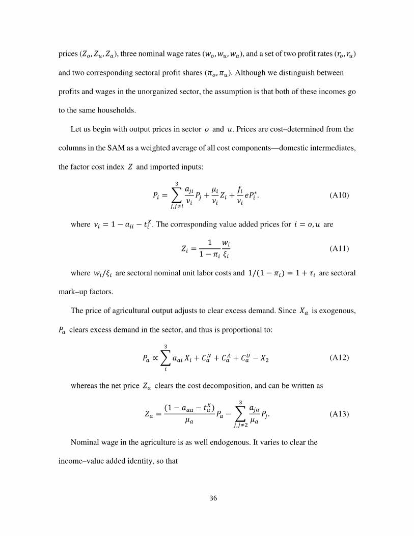
Sensitivity analysis

In this section we briefly discuss the relevance of several key parameters --

Kaldor-Verdoorn elasticities and price elasticities of import and export demand in the

organized and unorganized sectors. Figures 2 through 5 capture the effect of changing

elasticities on the real economy. The focus on growth rates of overall GDP and employment

in the organized sector. Shocks for all figures correspond to the simulation exercises in

Table 2. We discuss the two demand shocks but only one price shock—a nominal exchange

rate depreciation.

All figures show how the relevant variable (output or organized employment) is

changing in response to a varying parameter, given the shock. In all figures the values taken

by the key parameter appear on the horizontal axis, while the response of the variable is

plotted on the vertical axis.

Figures 2 and 3 correspond to the sensitivity analyses on trade elasticities in the

organized and unorganized and agricultural sectors respectively. As expected there is a

20

threshold above which a nominal depreciation becomes expansionary. This can be seen in

the top two diagrams of each figure. Given an exchange rate shock the simulation results are

more sensitive to changes in trade elasticities in the organized sector, but overall, the

magnitude of the expansion is larger in the presence of varying trade elasticities for the

unorganized sector. The economy responds visibly to changes in price elasticities of import

and export demand of organized sector when a demand shock is applied in either

sectors—the two lower panels (b.1,b.2, c.1, c.2) in Figure 2. The bottom line is that the larger

are price elasticities the more pronounced is the expansion. A positive demand shock

induces a rise in labor productivity through the Kaldor-Verdoorn rule which is set to 0.5 for

the organized sector and 0.2 for the unorganized sector. Consequently, there is a gain in

competitiveness which becomes ever more beneficial the higher is price elasticity of export

demand. In contrast to these results, different levels of elasticity in the unorganized sectors

produce no distinguishable reaction from the economy. The reason is that trade of

unorganized sector in the base year is only a fraction of the organized sector’s trade with the

rest of the world. Hence, its weight vis a vis trade and GDP is too small to make a visible

difference when its import and export demand elasticities are changing.

The effects of a varying Kaldor-Verdoorn coefficient in the organized sector are shown

in Figure 4. The relevant graphs for the unorganized sector are in Figure 5. Both sets of

results are obtained under the baseline configuration (3) for trade elasticities. What

transpires rather clearly is that the more sensitive labor productivity is to demand the more

pronounced is the slowdown in organized employment growth. This presents yet another

challenge for policy makers. On one hand a sustainable increase in incomes and especially

wages is not feasible in the long run without a rise in labor productivity as suggested by the

21

impact of a nominal wage shock in the previous section. On the other hand, labor

productivity increases reduce the need for employment growth and therefore stifles

structural change.

India in the world economy

What does India’s rise mean for the world economy? What role can India play in support

of global growth? These and related questions are addressed in this and a subsequent section

with a model for the world economy. The motivation is simple, and can be looked at from (at

least) two different angles. First, the global financial crisis, emanating from the US, had

large output effects both in the US and Europe. The question arose whether fast growing

large emerging economies would be able to decouple from these adverse shocks. Second,

both US and European economies remain weighed down by the toxic combination of

balance-sheet recessions and fiscal contraction. The question arises whether fast growing

large emerging economies will be able to sustain global growth; i.e. become an engine of

demand. These fast growing large emerging economies are of course the BRICs: Brazil,

Russia, India, China.

The following section presents a real-side one sector multi-country model of the world

economy with demand-determined output, bargained distribution and endogenous

productivity. The model is used further below for simulation analysis of BRICS country

performance. The exposition proceeds along the following steps: First, we present a one

country version in two dimensions—with all the necessary (and defensible) simplifications.

The purpose is to expound the core theoretical structure of the model. We briefly discuss the

multi-country model as well as the underlying data. In the following section, we motivate

and analyze relevant simulations.

22

A global model

The model covers product and labor markets in simple but comprehensive fashion. Let

us consider price and quantity setting in both markets.8 Product markets feature a

“macroeconomic firm” that uses domestic factors and imported intermediates from all other

regions to produce domestic value added. The firm marks up on domestic labor costs; the

supply price is then a weighted average of domestic factor and import cost. Foreign cost

pass-through is limited by the cost structure. The size of the mark-up depends on the degree

of competition in product markets. If the firm faces little competition and as a result has high

pricing power, its mark-up rate is high. High mark-ups, of course, imply high profit shares.

The level of aggregate demand for the firm’s product is a function of expenditure levels,

the multiplier and the real exchange rate. Expenditure levels—real private investment and

real public expenditures—are exogenous in this model. The multiplier, however, increases

with redistribution towards wage earners, due to their lower propensity to save. In that

fashion, expenditures, prices and distribution all affect the level of demand, and household’s

income.

There are two households, workers and capital owners. The two bargain in labor markets

over nominal wages, the single argument being the rate of unemployment. The lower the rate

of unemployment, the higher nominal wages, and vice versa. Further, labor productivity

depends on demand conditions, due to labor hoarding as well as overhead labor. Labor

hoarding refers to the fact that the firm retains skilled employees throughout a downturn

because retraining new employees in the upturn would be costlier; overhead labor refers to

the fact that firms usually have some back-office and managerial staff not easily made

8 The discussion of the model here largely follows von Arnim (2010) and von Arnim (2011). Financial support

from the International Institute for Labour Studies (IILS, ILO) for those studies is gratefully acknowledged.

23

expendable. The ratio of the real wage and labor productivity is equal to real unit labor cost,

or, in other words, the wage share.

We can think through an example to tie it all together. Suppose that business confidence

improves and investment increases. Unemployment decreases with the expansion of

demand. As just laid out, nominal wages rise. Output prices rise, but moderately, so that real

wages increase. On the other hand, productivity increases as well with the expansion of

demand. Whichever increases faster determines whether the distribution of income tilts in

favor of owners or workers. Internationally, the increase in demand leads to higher imports.

The rise in prices domestically leads to some real appreciation, which further increases

imports—and decreases exports. The fall in the current account is equivalent to a rise in

capital inflows, which in part finance the original outlays for business investment. Below we

present a stylized one country model in order to set the stage for what follows in

multi-country contexts further below. The model is presented in two dimensions: the rate of

utilization and the labor share.9

Let us begin with the components of effective demand:

# = $% = (1 − &'())� (1)

+ = �/, = + (2)

. = (/ − 0)/, = .'�, (), (3)

where #, +, . are consumption 2, (gross) investment � and net exports / − 0 relative

to capital stock ,. #, .are functions of the rate of utilization � = 3/, and the labor share

(.10

The signs of the partial derivates of these demand functions are standard: &4 < 0, since

9 The relevant literature is long; it shall suffice here to mention Rowthorn (1982), Dutt (1984), Taylor (1985),

Bhaduri & Marglin (1990) and Barbosa & Taylor (2007) as selected seminal papers. 10

The rate of utilization is proxied by the income-capital ratio. The actual rate of utilization is the ratio of

24

redistribution towards wage earners reduces the average savings propensity;.� > 0 through

the import channel, and .4 < 0 through the export channel, since higher real unit labor

costs represent a loss of price competitiveness.

Real unit labor costis defined as ( = 789: = ;< ,where

= = >/� = ='�, () (4)

? = 3/@ = ?'�, (), (5)

meaning both the real wage = and labor productivity ? are functions of the rate of

utilization and costs.The real wage responds positively to demand (=� > 0) due to the link

from goods to labor markets. Higher demand leads to higher activity, which necessitates

hiring—which in turn improves employee's bargaining position. Thus, the relevant variable

is the employment rate, but for the sake of simplicity, the chain of causation is summarized

here by �. Workers, obviously, can bargain only for nominal wages, so to simplify in this

manner it is further necessary to assume that firms can recoup at most a fraction of nominal

wage increases by price rises, and that these are anticipated.Further, the real wage responds

positively to labor productivity, =< > 0. Simply put, workers demand to share productivity

gains; such bargaining behavior is observed and is consistent with the desire (and tendency)

to maintain stable income shares. It implies that the real wage responds negatively to the

labor share, =4 < 0. In other words, elevated real unit labor costs—high real wages

relative to labor productivity—lead to decreases in real wages, and vice versa.

Labor productivity, in turn, is a positive function of demand along well known lines.

Okun’s Law provides empirical evidence for a short-run positive relationship between

current to full employment output; multiplying it by the (constant and normalized to unity) full

employment-capital ratio we get u as defined.

25

economic activity and labor productivity. It is primarily due to labor hoarding: Firms retain

skilled and overhead labor in a downturn, and as they are “getting busy again” in the upturn,

average employee productivity rises. Kaldor-Verdoorn effects are relevant over longer time

horizons, and due to specialization, learning by doing etc. In summary, ?� > 0. Further,

labor productivity responds positively to costs, ?4 > 0: High real unit labor costs provide

incentives for firms to “squeeze labor for effort,” rather than hire.

To assess characteristics and stability of the model, let us specify functions for the time

rate of change A�/AB = �C and A(/AB = (C :

�C = D(�E − �) = D((1 − &'())� + + + .'�, () − �) (6)

(C = G((E − () = G H;'�,4)<'�,4) − (I, (7)

where �E and (E are the rate of utilization and the labor share implied by effective

demand and distribution (real wage bargaining and productivity). The change in � and (

follows as the difference between these and current levels of output and the prevailing

distribution, respectively. The speed of adjustment depends on the magnitude of

sign-preserving coefficents D, G > 0. �C is a standard excess demand function, and (C is a

partial adjustment equation for the labor share. The Jacobian matrix (with D = G = 1

without loss of generality) of this two-dimensional system of differential equations is

J = K.� − & .4 − &4�=� 4; − ?� 4< =4 4; − ?4 4< − 1L = MN�CN� < 0 N�CN4 ≷ 0 PL/WLN4CN� ≷ 0 FS/PS N4CN4 < 0 U (8)

The top left entry is the dynamic multiplier. For stability in the goods market, it must be

negative; meaning the sum of the propensities to save (&) and import (.� < 0) must be

negative. The bottom right entry describes distributive own-feedback. For stability, its sign

26

must be negative. Since =4 < 0 and ?4 > 0, it must be negative.The off-diagonal entries

describe cross feedbacks. On the top right, (net) export response to labor share increases is

negative, but−&4� > 0, so that the aggregate sign depends on relative magnitudes. As is

standard in the Neo-Kaleckian literature, an overall negative (positive) sign denotes

profit-led (wage-led) demand. Second, on the bottom left, both real wages and productivity

respond positively to higher demand. The sign of the entry will depend on the relative

magnitudes of the two effects. A positive sign suggests successful employee bargaining, a

negative sign suggests successful firm bargaining, relative to demand-induced productivity

gains. The former is often labelled as a profit squeeze, the latter as forced

saving—summarized in the inequalities of the Jacobian above.

For stability, the determinant of the Jacobian must be positive, |J| > 0, and the trace of

the Jacobian must be negative, V'J) < 0. The latter will always be satisfied, since both

entries along the main diagonal are less than zero. The determinant will be positive if the

off-diagional entries are of opposite sign or small relative to the main diagonal.

From this one-sector one-country model, it is fairly straightforward to transition to the

multi-country model. The equations of the multi-country model are presented in Table 3.

Importantly, all equations are specified in levels, rather than rates of change.11

The dynamic

specification above provided simple conclusions on behavior and stability for the

one-country model. However, the dynamics evolve around an equilibrium, so that the

comparative static exercises of the static multi-country model are qualitatively the same. For

11The model falls within the general category of empirical economy-wide models, often labeled Computable

General Equilibrium (CGE) models. A CGE model is based on a Social Accounting Matrix (SAM), which

depicts detailed data on relations of production and distribution between main socio-economic agents in an

economy. The model adds behavioral relationships to the accounting; econometric evidence is applied to

calibrate relevant parameters. The complete model can then be used to calculate counterfactuals in response to

assumed shocks and policies. For standard discussions of the methodology, see Robinson (2003) and Taylor

(2004).

27

stability, it is sufficient to have positive multipliers in all countries, and not to have “large”

distributive feedbacks. Of course, the larger model permits endogenous determination of

prices: bargaining concerns nominal wages; and, given the mark-up, firms pass on changes

in nominal unit labor costs.12

The global data set covers a large share of the world’s national economies—one hundred

and sixty countries. Their relative size and their geographical trade relationships play a

crucial role. The model dataset is aggregated into sixteen countries and regions; the

countries are US, Japan, Canada, and the BRICS (Brazil, Russia, India, China and South

Africa),13

the regions Africa, Asia, Eurozone, the rest of Europe, and Latin America and the

Carribean. Countries with more than half of their exports concentrated in petroleum and

related products as well as natural gas are grouped together. Asia and the Eurozone are

further disaggregated into surplus and deficit regions. The principal source for the bilateral

trade matrix is the IMF’s Direction of Trade Statistics. The trade data is presented by

“reporting countries” and “partner countries” for exports and imports. Labor market data is

summarized by the unemployment rate. It is based on population, labor force, employment

and unemployment data from national statistics offices, regional development banks as well

as ILO’s Laborsta and EAPEP databases. Reported unemployment rates are used where

available, estimates based on the highest quality underlying data where not. For most data,

the base year is 2008. For a thorough discussion of the data set, see the appendix in von

12 The nominal wage increases with higher labor productivity. In the model above, that was expressed through

a negative response of the real wage to the wage share. Here, the nominal wage is a positive function of

employment rate and labor productivity. Labor productivity, in turn, depends in standard fashion on demand

conditions, due to labor hoarding as well as overhead labor—but further increases in the real wage. Since value

added (and output) prices follow “passively,” this setup produces a positive feedback between real wages and

labor productivity. 13

The original BRICs do not include South Africa. Since South Africa is so crucial an economy on the African

continent, it is included here as a single country.

28

Arnim (2010).

Simulations and discussion

Let us restate the central question to be addressed here: What does India’s rise mean for

the world economy? What role can India—and other BRIC countries—play in support of

global growth? To anticipate our conclusions: Probably a limited role. While growth in

many emerging markets has remained strong or recovered quickly, it appears that this might

be due in large part due to successful stimulus efforts. Global demand links from and to

BRIC countries are still weak relative to global demand links from and to US and Europe.

We can have a first look at this through the lens of linkage analysis. The method was

suggested in

Chenery & Watanabe (1958) and, for example, further developed in Syrquin &Chenery

(1989). Usually, the goal is to identify strength of inter-sectoral demand links in an

input-output table. Here, we apply the same concepts to the trade matrix to identify

backward and forward demand linkages between a set of countries and regions.

Linkages through trade

Direct backward (forward) linkages are column (row) sums of the trade flow matrix

divided by column (row) country. Indirect backward (forward) linkages are column (row)

sums (� − 0)WX, where � is the identity matrix and 0 the trade flow matrix scaled by

column (i.e. importing) country. Direct and indirect linkages are weighted by country GDP

(relative to US GDP), and then normalized around zero: A positive and high value indicates

existing and strong linkages. Backward linkages indicate the impact of a unit increase of

demand of a country on all other countries; forward linkages indicate the impact of a unit

increase of demand in all other countries on the country under consideration. Put differently,

29

backward linkages show a demand “pull” effect—the degree to which a country’s growth

requires other countries’ outputs, and forward linkages a demand “push” effect—the degree

to which a country’s output is required as in input to other countries’ growth.

Table 4 summarizes results: Europe and US have very strong backward and forward

linkages. The BRICs appear in the lower part of the table; all with very weak linkages. China

proves the exception: the manufacturing giant’s large trade surplus implies at least weak

forward linkages. (The countries and regions are ranked by the sum of the averages of direct

and indirect backward and forward linkages, thus measuring the overall importance through

demand “pull and push” effects.) The ranking in the table is dominated by country GDP size.

The larger a country’s GDP, the greater the weight on the linkages. Unweighted linkage

measures, however, indicate the impact of a unit change of the country’s GDP. Weighted

linkage measures indicate the impact of such a change relative to world GDP, which is

obviously the relevant metric. It follows that the ranking in the table is influenced as well by

the aggregation scheme. Individual European countries would be ranked lower than if

weighing in as a bloc.

It does, however, make sense to use this aggregation scheme. Obviously, the US features

large as an individual country. Europe acts globally as a trading bloc, rather than individual

countries; and it has a single currency. This does not apply to the same degree to the

composite region of Asia, but the relevant comparison is between US and Europe on the one

hand, and individual BRIC countries on the other. In summary, US and Europe tend to

benefit strongly from global growth through forward linkages, and the world benefits from

US and European growth through backward linkages. The reverse conclusion matters in

current circumstances: US and Europe in recession limit global growth. Growth in the BRIC

30

countries and especially India, on the other hand, has only a limited impact on global growth.

Demand shocks: Local and global impact

Simulation results confirm these insights.14

Tables 5 and 6 summarize simulation results

for an investment expansion in BRIC countries and the developed world, respectively. In

both cases, investment in each country is increased by one percent of GDP, simply to

compare the global effects of growth in the BRIC countries and the developed world (US,

Europe, Japan).

In the “BRIC growth” scenario, BRIC countries experience growth. Since wages and

prices (and real wages) are pro-cyclical, all countries see some real appreciation. The

price-adjusted multiplier, however, is still larger than one in all countries. Across the four

BRIC countries, the external balance relative to GDP worsens: capital inflows must partially

finance the private investment increase. The private balance (saving—investment) relative

to GDP falls. The expansion increases government revenue, so that with constant real public

expenditures the public balance improves. (Overall, the sum of the changes in public and

private balances is equal to the change in the foreign balance.) Crucially, the model suggests

that BRIC growth leads to negligible developed country growth, and that global growth is

very weak.

In sharp contrast, the “developed country growth” scenario shows not only significant

global growth but as well growth in the developing world—including the BRIC countries.

To be sure, the result is driven by the relative size of developed economies, which implies

that the one-percent-of-GDP investment expansion is larger in absolute terms. That,

however, is exactly the point: A “regular” expansion in these regions has a significant

14 We will not discuss model calibration here. Von Arnim (2010, 2011) present details on behavioral

parameters as well as sensitivity analysis.

31

impact on BRIC countries and the rest of the world, whereas the same cannot be said to

apply in reverse. Furthermore, due to strong backward linkages especially from US and

Europe to the rest of the world, repercussion multipliers lead to a strong full multiplier (in

excess of two) in the developed world. (Repercussion multipliers include the positive

demand effect from abroad after a domestic positive demand shock.) In summary, the model

suggests that growth (or the lack thereof) in developed countries has relatively strong

positive (adverse) affects in BRIC countries.

Tables 7-10 further corroborate these results. Each of these tables focuses on a demand

injection in one BRIC country in detail. Figure 6 provides a different look at the same theme.

The chart summarizes model results in response to a one-percent-of-GDP investment shock

in each region or country. The statistic considered is global real GDP growth (top left cell in

the tables above), indexed by Europe’s result. As an example, consider Japan: A positive

investment demand shock of 1% of Japan’s GDP in Japan leads to global real GDP growth

roughly one quarter as strong as a positive investment demand shock of 1% of Europe’s

GDP in Europe. The BRICs rank low, and India third from the bottom—in line with relative

GDP size.

To conclude, BRIC countries might well matter at the margin for global growth.

Certainly, BRIC country growth matters greatly for BRIC country residents. But overall,

growth from a lower base and with still weaker trade links suggests that talk of

decoupling—in the sense of being shielded from US and Europe recessions as well as acting

as a global growth engine—is premature.

Conclusions

This paper addresses India’s structural transformation and role in the world economy.

32

India’s accelerated growth in recent years has lead to much praise, but as well to questions

about sustainability, resilience and inclusiveness of that performance. Based on simulation

results from the structuralist three sector model of development employed here, sustained

growth requires strengthened links between formal and informal activities. Further, based on

simulation results from a global model with demand determined output and distributive

bargaining, India—and other BRIC countries—are unlikely to take over as engines of

growth in the world economy. Their relative size is still too small; indeed, the lack of global

linkages suggests that the old adage of the US sneezing and the world catching a cold might

still matter.

Appendix: A three-sector model

The three-sector model adopted in this paper borrows the modeling framework and setup

from von Arnim & Rada (2011). At the origin it is the standard fixed-flex price model

developed by Taylor (1983) and later explored by Rada (2007) and Rada & von Arnim

(forthcoming).

The structure of the economy is presented in the SAM in Table 1 and has been briefly

discussed above. The data comes from Saluja & Yadav (2006) and Ojha et.al. (2009). We

focus on three productive sectors: (1) organized activities, (2) agriculture and (3)

unorganized non-agricultural activities; and six institutional sectors—four types of

households, government and the rest of the world.

The SAM meets the basic accounting constraints. The NW three by three matrix is the

input-output table which captures intermediate demands. Along the top three rows we have

final sales by sectors, while along the three columns we observe production

costs—intermediates, factor costs, production taxes (net of subsidies), and imports.

33

Transfers from government and from the rest of the world to households are found in the

middle cells of the SAM. Lastly, the Y�Y row capture saving by each institutional sector.

Organized and unorganized activities are similar in the sense that each are assumed to

hold excess capacity and that each can take advantage of dynamic economies of scale as

captured by the Kaldor-Verdoorn effects. As discussed by von Arnim & Rada (2011) the

assumption of a fixed technology and limited fertile land implies that agricultural output is

pre–determined, and does not vary with changing levels of labor supply. Agricultural labor

productivity is endogenous, and responds negatively to a demand expansion in the other

sectors which leads to hiring there, and therefore to a reduction of surplus labor in

agriculture. However, average labor productivity increases automatically such that

agricultural output, indeed, remains constant.

The above story can be specified formally as follows. Let 3 be the real GDP and @ an

index of total employment. We define the level of labor productivity as ?8 = :8 which

through log–differentiation leads to its growth rate ex-post:

?Z8 = 3[ − @[,  (A1)

where a "hat" over a variable indicates the growth rate of said variable. Adopting the

Kaldor-Verdoorn specification for labor productivity in the organized and unorganized

sectors we get:

?8] = �^3]_` (A2)

where the sub–index i denotes the sector, �^ is the productivity trend and �] is the

sectoral demand elasticity of productivity. The behavioral function (2) means in growth

terms that ?Z] = �Z^ + �]3[]and further that employment in the sector a follows from

@[] = 3[] − ?Z8], or, in level terms:

34

@] = �WX3]XW_`  (A3)

for a = �, �, where ?] is sectoral labor productivity. For the agriculture the relevant closure

is:

?� = 3�@�  (A4)

where 3� is pre-determined in real terms and @� is obtained as a residual after employment

in the organized and unorganized sectors have been calculated according to (A3).

Output and employment

Real output in the organized and unorganized sectors b] is calculated from the demand

side as the sum of intermediate demands, consumption 2]c where d specifies the type of

household, investment �], government expenditures !] and exports /]:

b] = e �]cfc b^ + 2]c + !] + �] + /] where i = o, u, and j

= o, u, a

(A5)

Total consumption of the sector’s product decomposes by sources of demand, 2] = 2]� +2]� + 2]�, where subscripts denote the type of product, and (capitalized) superscripts the

origin of demand for that product in this case the three consuming households

—wage-earning households from the organized sector, agricultural households and

unorganized households respectively. We provide further details on the specification of the

consumption functions later on. Unlike the organized and unorganized sectors, the level of

agricultural output is capacity–constrained, and just proportional to inherited capital:

b� = r,� = bs�  (A6)

Value added in the three sectors is proportional to real outputs. Having used already the

35

degree of freedom from the cost decomposition along each sector’s column for the

determination of the output price, we adopt a behavioral relationship to determine the

sectoral value added. We can write the share of domestic value added in supply as:

tc = 3cbc = 1 − Me �c]fc + Bcu + vc�U  where i = j = o, u, a  (A7)

where Bcu is a production tax net of subsidies, vc = 0c/bc is the sectoral import propensity

and �is the nominal exchange rate, quoted as the domestic currency price of a unit of foreign

currency. Further, value added is then determined from 3c = wcbc. Unless either the

nominal exchange rate � or vc varies, wc takes the base year value.

Next, and identical to von Arnim & Rada (2011), trade responds to price changes based

on standard specifications:

0c = �c �cWxybc (A8)

/c = �c �czybc{ ,  (A9)

where ��c∗ is the foreign price of tradable goods expressed in the domestic currency, �c

is the domestic goods price, and �c = |9y∗9y is the sector’s relative price or a measure of the

real exchange rate. Price elasticities of import demand �c and export demand �c can vary

substantially across sectors and are some of our key parameters in the model.

Lastly, and as already stated, investment and government expenditures on industry

output are exogenous. Consumption is determined by a standard Linear Expenditure System

(LES) as explained below.

Prices and distribution

The model features three sectoral output prices (�� , ��, ��), three sectoral value added

36

prices ("� , "�, "�), three nominal wage rates (>� , >�, >�), and a set of two profit rates (V� , V�)

and two corresponding sectoral profit shares (}� , }�). Although we distinguish between

profits and wages in the unorganized sector, the assumption is that both of these incomes go

to the same households.

Let us begin with output prices in sector � and �. Prices are cost–determined from the

columns in the SAM as a weighted average of all cost components—domestic intermediates,

the factor cost index " and imported inputs:

�] = e �c].]f

c,c~] �c + t].] "] + v].] ��]∗.  (A10)

where .] = 1 − �]] − B]u. The corresponding value added prices for a = �, � are

"] = 11 − }]>]?]   (A11)

where >]/?] are sectoral nominal unit labor costs and 1/(1 − }]) = 1 + �] are sectoral

mark–up factors.

The price of agricultural output adjusts to clear excess demand. Since b� is exogenous,

�� clears excess demand in the sector, and thus is proportional to:

�� ∝ e ��]f] b] + 2�� + 2�� + 2�� − b�  (A12)

whereas the net price "� clears the cost decomposition, and can be written as

"� = (1 − ��� − B�u)t� �� − e �c�t�f

c,c~� �c . (A13)

Nominal wage in the agriculture is as well endogenous. It varies to clear the

income–value added identity, so that

37

>� = "�3�@� = ��?�  (A14)

Hence, the real wage per worker expands at the same pace as the labor productivity in the

sector, which itself is determined by the flow of labor to and from the agricultural sector. In

summary, �� responds to demand; "� responds net income per unit, in other words, to the

excess of �� over costs; and >� responds to "� and labor productivity.

Nominal wages in the other two sectors are exogenous, but profit rates vary with the

distribution of income and economic activity as in the standard Kaleckian models. The two

sectoral profit rates are allowed to differ. From the definition of the capital share, the profit

rates can then be written as

V� = }� "�3���,�  and (A15)

V� = }� "�3���,� .  (A16)

The mark–up rates �� and �� are exogenous, implying that the distribution of factor

income in these two sectors is exogenous. The overall profit share } is just total profit

income as a share of aggregate GDP, ��3. The GDP–deflator �� is calculated as a

Fisher–index of the three sectoral prices (see von Arnim & Rada (2011) for details).

Consumption equations

Demand functions for consumer households are derived from a standard Linear

Expenditure (LES) system. A generic system of demand for a three commodities economy

is:

2�c = #�c 3Ec − ��2�c�� (A17)

38

2�c = #�c 3Ec − ��2�c�� (A18)

2�c = (#�c + #�c)2�c + (1 − #�c − #�c) 3Ec�� . (A19)

where d is the type of household and 2�c is its consumption floor of agricultural product

which is assumed to be food or food-related, and 3E is the household’s disposable income.

Saving takes place in all households across sectors. The data for 2003-04 shows that

saving rates as a percentage of gross income, including transfers from the government and

the rest of the world, varies between 5 per cent of the income of some of the rural households

to over 30 per cent for the urban organized households or the self-employed.

A first assumption is that in the organized sector only the wage earners consume.

Organized working households disposable income is 3E� = (1 − B:� − &7� )((1 − }�)"�3� +Vw� + BV�), where }� = 1 − 7�8���:� is the sectoral capital share, B:� is the tax rate on sectoral

wage income, &7 is the saving rate of working households in the organized sector, and Vw�

and BV� are transfers from the rest of the world and government respectively. Organized

households demand all three goods, and consume a minimum "floor" amount of agricultural

product, 2��. Analogously, �– and �– households disposable income are 3E� = (1 − B:� −&�)"�3� + Vw� + BV� and 3E� = (1 − B:� − &�)"�3� + Vw� + BV� respectively, and their

floor consumption of agricultural product are 2�� and 2��.

Organized sector profit recipients, the 2–households, do not consume. Their income is

3$ = }�"�3� + BV�. Finally, profit income is taxed at the rate B:� .

39

References

Athukorala, P.-C. (2009). Outward foreign direct investment from india. Asian

Development Review, 26, no. 2:125–153.

Barbosa-Filho, N. H. and Taylor, L. (2007). Distributive and Demand Cycles in the

US-Economy—A Structuralist Goodwin Model. Metroeconomica, 57:389-411.

Bhaduri, A. and Marglin, S. (1990). Unemployment and the Real Wage: The Economic

Basis for Contesting Political Ideologies. Cambridge Journal of Economics,

14(4):375-393.

Breman, J. (2010). Indias’s social question in a state of denial. Economic and Political

Weekly, 45:42–46.

Chandrasekhar, C. P. and Ghosh, J. (2007). Recent employment trends in India and China:

An unfortunate convergence? Social Scientist, 35:19–46.

Chenery, H. B. (1960). Patterns of industrial growth. The American Economic Review,

50(4):624–654.

Chenery, H., Robinson, S., and Syrquin, M. (1987). Industrialization and Growth: A

Comparative Study. A World Bank Publication.

Chenery, H. B. & Watanabe, T. (1958). International Comparisons of the Structure of

Production. Econometrica, 26, 487-521

Deaton, A. and Drèze, J. (2002). Poverty and inequality in india: A reexamination.

Economic and Political Weekly, 7 September:3729–3748.

Dutt, A. K. (1984). Stagnation, Income Distribution and Monopoly Power. Cambridge

Journal of Economics, 8(1):25-40.

Gandolfo, G. (2010). Economic Dynamics. Springer, 4th edition.

Hicks, J. (1965). Capital and Growth. Oxford University Press.

Kaldor, N. (1966). Causes of the Slow Rate of Growth of the United Kingdom. Cambridge,

UK: Cambridge University Press, London.

Kalecki, M. (1976). Essays on developing economies. Humanities Press.

Mitra, A. (2011). Trade in services: Impact on employment in india. The Social Science

Journal, 48(1):72—93.

Naastepad, C. W. M. (2006). Technology, Demand and Distribution: A Cumulative Growth

Model with an Application to the Dutch Productivity Growth Slowdown. Cambridge

Journal of Economics, 30(3):403-434.

Ocampo, J. A. (2005). Beyond Reforms. Structural Dynamics and Macroeconomics

Vulnerability, chapter The Quest for Dynamic Efficieny: Structural Dynamics and

Economic Growth in Developing Countries, pages 3–43. Stanford University Press.

Ojha, V., Pal, B. D., Pohit, S., and Roy, J. (2009). Social accounting matrix for india. mime.

Pyatt, G. 1988. The SAM Approach to Modeling. Journal of Policy Modeling, 10, 327–352

Rada, C. (2007). Stagnation or Transformation of a Dual Economy through Endogenous

Productivity Growth. Cambridge Journal of Economics, 31:711–40.

Rada, C. (2010). Formal and informal sectors in China and India. Economic Systems

Research, 22:129–53.

Rada, C. and von Arnim, R. L. (forthcoming). Structural transformation in china and india:

A note on macroeconomic policies. Structural Change and Economic Dynamics.

Ranis, G., Stewart, F., and Ramirez, A. (2000). Economic growth and human development.

World Development, 28(2):197–219.

40

Robinson, S. 2003. Macro Models and Multipliers: Leontief, Stone, Keynes, and CGE

Models. International Food Policy Research Institute (IFPRI)

Rowthorn, R. E. (1982). Demand, Real Wages and Economic Growth. Studi Economici,

18:3-53.

Saluja, M. R. and Yadav, B. (2006). Social accounting matrix for india 2003-04. India

Development Foundation.

Sen, A. K. (1966). Peasants and dualism with or without surplus labor. Journal of Political

Economy, 74.

Syrquin, M. &Chenery, H. B. (1989) Patterns of Development, 1950 to 1983. World Bank.

Taylor, L. (1979). Macro models for developing countries. Mc.

Taylor, L. (1983). Structuralist Macroeconomics: Applicable Models for the Third World.

Basic Books.

Taylor, L. (1985). A Stagnationist Model of Economic Growth. Cambridge Journal of

Economics, 9:383-403.

Taylor, L. (2004). Reconstructing Macroeconomics: Structuralist Proposals and Critiques

of the Mainstream. Harvard University Press.

Trivedi, Pushpa,L. Lakshmanan, R. Jain and Y.K. Gupta (2012), Productivity, Efficiency

and Competitiveness of the Indian Manufacturing Sector, Study No. 37, Development

Research Group.

von Arnim, R. (2010) Employment prospects: A global model of recovery and

rebalancing.International Institute for Labour Studies (IILS, ILO) Discussion Paper

No.203

von Arnim, R. (2011) Core labor standards, wage-productivity linkages and growth. Mimeo,

International Institute for Labour Studies (IILS, ILO)

von Arnim, R. and Rada, C. (2011). Labour productivity and energy use in a three-sector

model: An application to Egypt.

Development and Change, 42(6):1323–1348.

41

Tables and figures

10 bill. Rs

Org

anized

Ag

ricultu

re

Un

org

anized

Org

-HH

Ag

ric-HH

Un

org

-HH

Cap

-HH

Go

vern

men

t

RO

W

Investm

ent

Total

Organized 623.9 64.1 544.1 149.3 154.7 322.5 151.4 337.9 359.5 2,707.3

Agriculture 83.7 146.3 86.4 81.1 127.7 194.2 719.3

Unorganized 447.2 57.3 423.5 150.3 154.8 324.3 153.7 73.8 364.9 2,149.7

W-agriculture 479.3

65.6 9.4

554.3

W-organized 733.2 58.7 38.9 830.8

W-unorganized 301.0 129.0 70.6 500.6

Profits 410.8 579.0

33.4

1,023.2

Government 120.4 (36.5) 65.9 66.0 34.2 42.8 63.6 49.8 406.3

ROW 288.1 8.9 149.9

446.9

FOF

384.3 82.9 195.6 380.7 (185.5) (83.7) 774.1

Total 2,707.3 719.3 2,149 830.8 554.3 1,079.6 444.2 406.3 446.9 774.1

Table 1: A Social Accounting Matrix for 2003-04. Source: Aggregation based on Ojha, V., Pal, B. D., Pohit, S., and Roy, J. (2009).

Social accounting matrix for India. mimeo, and Saluja, M. R. and Yadav, B. (2006). Social accounting matrix for india 2003-04. India

Development Foundation.

Figure 1: Simulation results. The rate of expansion in organized employment under different shock scenarios and calibrations.

42

Demand Wage Exchange rate

7% real investment

increase in the

organized sector

7% real

Investment

increase in the

unorganized sector

10% nominal wage

increase inthe

organized sector

10% nominal

exchange

depreciation (rise)

1 2 3 1 2 3 1 2 3 1 2 3

Macroeconomic statistics

Real GDP growth 1.1 1.2 1.3 1.4 1.4 1.5 -1.0 -1.0 -3.0 -2.8 -2.9 0.1

Inflation 0.6 0.1 0.1 0.9 0.4 0.4 4.6 5.2 5.3 -1.0 0.2 0.1

Real exchange rate -0.6 -0.1 -0.1 -0.9 -0.4 -0.4 -4.4 -4.9 -5.1 11.1 9.8 9.9

Private balance (∆ in % pts of GDP) -0.6 -0.7 -0.6 -0.7 -0.7 -0.7 0.5 0.5 0.0 -0.8 -0.7 0.1

Public balance (∆ in % pts of GDP) 0.4 0.3 0.3 0.4 0.4 0.4 0.5 0.5 0.1 -0.7 -0.6 0.1

External balance (∆ in % pts of GDP) -0.3 -0.4 -0.3 -0.3 -0.4 -0.3 1.0 1.1 0.1 -1.5 -1.3 0.2

Employment share of organized sec (∆ in % pts) 0.3 0.1 0.2 0.2 0.1 0.1 -0.2 -0.1 -0.4 -0.6 -0.3 0.1

Output share of organized sec(∆ in % pts) 0.3 0.3 0.4 -0.1 -0.1 -0.1 -0.3 -0.3 -0.9 -0.4 -0.5 0.3

Productivity

Organized & unorganized

Labor productivity growth - organized 0.0 0.9 1.0 0.0 0.6 0.7 0.0 -0.9 -2.5 0.0 -2.0 0.4

Labor productivity growth - unorganized 0.0 0.2 0.2 0.0 0.5 0.5 0.0 -0.1 -0.4 0.0 -0.6 -0.2

Agriculture

Labor productivity growth 0.8 0.5 0.6 1.3 1.0 1.0 -0.7 -0.5 -1.3 -2.3 -1.7 -0.3

Key parameters 1 2 3

Trade price elasticities in the organized sector 0 0 0.75

Trade price elasticities in the unorganized sector 0 0 0.30

Kaldor-Verdoorn elasticity organized 0 0.50 0.50

Kaldor-Verdoorn elasticity unorganized 0 0.20 0.20

Table 2: Simulation results (3-sector model). The simulations results are based on a three-sector model for India using data from a Social

Accounting Matrix or 2003-04. Four shocks are applied in the context of three different calibrations of key parameters. These parameters

and the values they take in each calibration are presented in the lower part of the table.

43

Figure 2: Sensitivity analysis on trade elasticities for the organized sector.

44

Figure 3: Sensitivity analysis on trade elasticities for the unorganized sectors (it includes agriculture).

45

Figure 4: Sensitivity analysis on Kaldor-Verdoorn coefficient for the organized sectors.

46

Figure 5: Sensitivity analysis on Kaldor-Verdoorn coefficient for the unorganized sectors (it includes agriculture).

47

�] = �1 − ∑ w]c�c�X ��] + ∑ w]c�c�X �]c�c (Equation 1: Supply or output price)

�] = '1 + �]) 7< = XXW�`7`<` (Equation 2: Mark-up price or GDP deflator)

>] = >]^ �8��7`� ?7`� (Equation 3: Nominal wage)

V] = }] �`:`9`%` (Equation 4: Profit rate)

}] = 1 − 7`8`�`:` = 1 − ;`<` (Equation 5: Profit share)

�] = ∑ B]c�]c�c�X (Equation 6: Trade-weighted nominal exchange rate

�] = ∑ B]c�]c 9y9`�c�X (Equation 7: Trade-weighted real exchange rate)

b] = 2] + �] + !] + /] (Equation 8: Real total supply)

2] = (1 − &] − B�])�]3]/�] (Equation 9: Real consumption)

3] = �](�] + !] + /]) (Equation 10: Real GDP)

�] = XW∑ �`y�y��XWHXW∑ �`y�y�� I(XW�`W��`)�`/9` (Equation 11: Multiplier)

0] = ∑ w]cb]�c�X = ∑ w]^�]cW�`yb]�`y�c�X (Equation 12: Real imports)

/] = ∑ wc]bc�c�X (Equation 13: Real exports)

B]c = 9`�y`uy |`y9y�`yu`9` ∑ �y`uy�y��  ∑ |`y9y�`yu`�y�� (Equation 14: Trade share)

�] = &]�]3] = �&]� − ¡&]� − &]4¢(1 − }])��]3] (Equation 15: Private saving)

�]£ = B�]�]3] − �]!] (Equation 16: Government (dis)saving)

?] = ?]^ �:`%`�<`� �7`�`�<`� (Equation 17: Labor productivity)

@] = :`<` (Equation 18: Employment)

2�] = �] ∑ wc]bc�c�X − ∑ �]c�cw]cb]�c�X = −�]{ (Equation 19: Current Account)

Table 3: Overview of model equations used for simulations. The model is identical to the one used in von Arnim (2011).

Backward

Direct Indirect

EUROPE 1.67 2.85

US 1.61 2.02

ASIA 0.88 0.23

ENERGY 0.32 -0.24

CHINA -0.02 0.02

JAPAN -0.22 0.04

LAC -0.26 -0.46

CANADA -0.43 -0.64

RUSSIA -0.52 -0.63

BRAZIL -0.68 -0.67

INDIA -0.69 -0.72

AFRICA -0.81 -0.86

S.

AFRICA -0.86 -0.93

Table 4: Trade linkages in the world economy.

divided by column (row) country. Indirect backward (forward) linkages are column (row) sums

and ¤ the trade flow matrix scaled by column (i.e. importing) country. Direct and indirect linkages are weighted by country GDP (re

to US GDP), and then normalized around zero: A positive and high value ind

highlighted in grey.

Figure 6: Simulation results. This chart summarizes model results in response to a one

respective region or country. The statistic considered here is global real GDP growth (top left cell in the tables above),

result. As an example, consider Japan: A positive investment demand shock of 1% of Japan’s GDP in

growth roughly one quarter as strong as a positive investment demand shock of 1% of Europe’s GDP in Europe.

48

Forward

Average Direct Indirect Average TOTAL

2.26 1.45 4.11 2.78 5.04

1.82 0.66 2.12 1.39 3.21

0.56 0.81 0.03 0.42 0.97

0.04 0.88 -0.39 0.25 0.29

0.00 0.53 -0.10 0.21 0.21

-0.09 -0.02 -0.14 -0.08 -0.17

-0.36 -0.30 -0.64 -0.47 -0.83

-0.54 -0.43 -0.78 -0.60 -1.14

-0.58 -0.40 -0.76 -0.58 -1.16

-0.67 -0.72 -0.77 -0.74 -1.42

-0.70 -0.72 -0.81 -0.77 -1.47

-0.84 -0.85 -0.91 -0.88 -1.72

-0.89 -0.89 -0.96 -0.92 -1.82

: Trade linkages in the world economy. Direct backward (forward) linkages are column (row) sums of the trade flow matrix

divided by column (row) country. Indirect backward (forward) linkages are column (row) sums (¥ − ¤)W¦, where ¥

the trade flow matrix scaled by column (i.e. importing) country. Direct and indirect linkages are weighted by country GDP (re

to US GDP), and then normalized around zero: A positive and high value indicates existing and strong linkages. BRIC countries are

This chart summarizes model results in response to a one-percent-of-GDP investment shock in each

untry. The statistic considered here is global real GDP growth (top left cell in the tables above),

. As an example, consider Japan: A positive investment demand shock of 1% of Japan’s GDP in Japan leads to global real GDP

growth roughly one quarter as strong as a positive investment demand shock of 1% of Europe’s GDP in Europe.

Classification

Very strong

Very strong

Strong

Strong

Weak

Weak

Weak

Very weak

Very weak

Very weak

Very weak

Very weak

Very weak

Direct backward (forward) linkages are column (row) sums of the trade flow matrix

is the identity matrix

the trade flow matrix scaled by column (i.e. importing) country. Direct and indirect linkages are weighted by country GDP (relative

icates existing and strong linkages. BRIC countries are

GDP investment shock in each

untry. The statistic considered here is global real GDP growth (top left cell in the tables above), indexed by Europe’s

apan leads to global real GDP

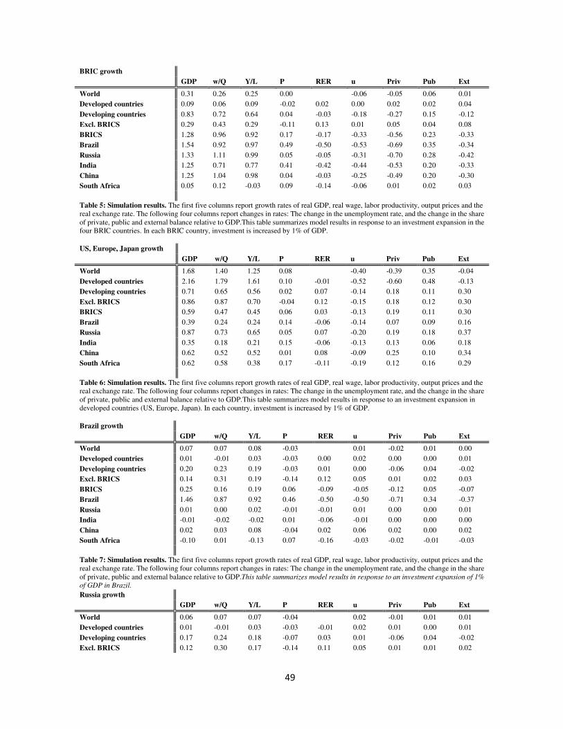
49

BRIC growth

GDP w/Q Y/L P RER u Priv Pub Ext

World 0.31 0.26 0.25 0.00 -0.06 -0.05 0.06 0.01

Developed countries 0.09 0.06 0.09 -0.02 0.02 0.00 0.02 0.02 0.04

Developing countries 0.83 0.72 0.64 0.04 -0.03 -0.18 -0.27 0.15 -0.12

Excl. BRICS 0.29 0.43 0.29 -0.11 0.13 0.01 0.05 0.04 0.08

BRICS 1.28 0.96 0.92 0.17 -0.17 -0.33 -0.56 0.23 -0.33

Brazil 1.54 0.92 0.97 0.49 -0.50 -0.53 -0.69 0.35 -0.34

Russia 1.33 1.11 0.99 0.05 -0.05 -0.31 -0.70 0.28 -0.42

India 1.25 0.71 0.77 0.41 -0.42 -0.44 -0.53 0.20 -0.33

China 1.25 1.04 0.98 0.04 -0.03 -0.25 -0.49 0.20 -0.30

South Africa 0.05 0.12 -0.03 0.09 -0.14 -0.06 0.01 0.02 0.03

Table 5: Simulation results. The first five columns report growth rates of real GDP, real wage, labor productivity, output prices and the

real exchange rate. The following four columns report changes in rates: The change in the unemployment rate, and the change in the share

of private, public and external balance relative to GDP.This table summarizes model results in response to an investment expansion in the

four BRIC countries. In each BRIC country, investment is increased by 1% of GDP.

US, Europe, Japan growth

GDP w/Q Y/L P RER u Priv Pub Ext

World 1.68 1.40 1.25 0.08 -0.40 -0.39 0.35 -0.04

Developed countries 2.16 1.79 1.61 0.10 -0.01 -0.52 -0.60 0.48 -0.13

Developing countries 0.71 0.65 0.56 0.02 0.07 -0.14 0.18 0.11 0.30

Excl. BRICS 0.86 0.87 0.70 -0.04 0.12 -0.15 0.18 0.12 0.30

BRICS 0.59 0.47 0.45 0.06 0.03 -0.13 0.19 0.11 0.30

Brazil 0.39 0.24 0.24 0.14 -0.06 -0.14 0.07 0.09 0.16

Russia 0.87 0.73 0.65 0.05 0.07 -0.20 0.19 0.18 0.37

India 0.35 0.18 0.21 0.15 -0.06 -0.13 0.13 0.06 0.18

China 0.62 0.52 0.52 0.01 0.08 -0.09 0.25 0.10 0.34

South Africa 0.62 0.58 0.38 0.17 -0.11 -0.19 0.12 0.16 0.29

Table 6: Simulation results. The first five columns report growth rates of real GDP, real wage, labor productivity, output prices and the

real exchange rate. The following four columns report changes in rates: The change in the unemployment rate, and the change in the share

of private, public and external balance relative to GDP.This table summarizes model results in response to an investment expansion in

developed countries (US, Europe, Japan). In each country, investment is increased by 1% of GDP.

Brazil growth

GDP w/Q Y/L P RER u Priv Pub Ext

World 0.07 0.07 0.08 -0.03 0.01 -0.02 0.01 0.00

Developed countries 0.01 -0.01 0.03 -0.03 0.00 0.02 0.00 0.00 0.01

Developing countries 0.20 0.23 0.19 -0.03 0.01 0.00 -0.06 0.04 -0.02

Excl. BRICS 0.14 0.31 0.19 -0.14 0.12 0.05 0.01 0.02 0.03

BRICS 0.25 0.16 0.19 0.06 -0.09 -0.05 -0.12 0.05 -0.07

Brazil 1.46 0.87 0.92 0.46 -0.50 -0.50 -0.71 0.34 -0.37

Russia 0.01 0.00 0.02 -0.01 -0.01 0.01 0.00 0.00 0.01

India -0.01 -0.02 -0.02 0.01 -0.06 -0.01 0.00 0.00 0.00

China 0.02 0.03 0.08 -0.04 0.02 0.06 0.02 0.00 0.02

South Africa -0.10 0.01 -0.13 0.07 -0.16 -0.03 -0.02 -0.01 -0.03

Table 7: Simulation results. The first five columns report growth rates of real GDP, real wage, labor productivity, output prices and the

real exchange rate. The following four columns report changes in rates: The change in the unemployment rate, and the change in the share

of private, public and external balance relative to GDP.This table summarizes model results in response to an investment expansion of 1%

of GDP in Brazil.

Russia growth

GDP w/Q Y/L P RER u Priv Pub Ext

World 0.06 0.07 0.07 -0.04 0.02 -0.01 0.01 0.01

Developed countries 0.01 -0.01 0.03 -0.03 -0.01 0.02 0.01 0.00 0.01

Developing countries 0.17 0.24 0.18 -0.07 0.03 0.01 -0.06 0.04 -0.02

Excl. BRICS 0.12 0.30 0.17 -0.14 0.11 0.05 0.01 0.01 0.02

50

BRICS 0.22 0.19 0.19 -0.01 -0.03 -0.02 -0.12 0.06 -0.07

Brazil 0.00 0.01 -0.01 0.00 -0.05 -0.01 0.00 0.00 0.00

Russia 1.23 1.03 0.92 0.04 -0.07 -0.29 -0.72 0.26 -0.45

India -0.02 -0.03 -0.03 0.01 -0.07 -0.01 0.00 0.00 0.00

China 0.02 0.03 0.09 -0.05 0.01 0.06 0.02 0.00 0.02

South Africa -0.11 0.00 -0.14 0.06 -0.17 -0.03 -0.02 -0.01 -0.03

Table 8: Simulation results. The first five columns report growth rates of real GDP, real wage, labor productivity, output prices and the

real exchange rate. The following four columns report changes in rates: The change in the unemployment rate, and the change in the share

of private, public and external balance relative to GDP.This table summarizes model results in response to an investment expansion of 1%

of GDP in Russia.

India growth

GDP w/Q Y/L P RER u Priv Pub Ext

World 0.05 0.05 0.06 -0.03 0.02 -0.01 0.01 0.00

Developed countries 0.00 -0.01 0.02 -0.03 0.00 0.02 0.00 0.00 0.00

Developing countries 0.15 0.19 0.16 -0.05 0.02 0.01 -0.03 0.02 -0.02

Excl. BRICS 0.13 0.30 0.18 -0.14 0.11 0.05 0.01 0.02 0.02

BRICS 0.16 0.11 0.14 0.03 -0.06 -0.02 -0.07 0.02 -0.06

Brazil -0.01 0.00 -0.02 0.00 -0.04 -0.01 0.00 0.00 0.00

Russia 0.01 0.00 0.02 -0.02 -0.01 0.01 0.00 0.00 0.00

India 1.16 0.66 0.72 0.38 -0.43 -0.41 -0.56 0.19 -0.37

China 0.02 0.03 0.08 -0.05 0.02 0.06 0.02 0.00 0.02

South Africa -0.08 0.02 -0.12 0.07 -0.16 -0.03 -0.01 -0.01 -0.02

Table 9: Simulation results. The first five columns report growth rates of real GDP, real wage, labor productivity, output prices and the

real exchange rate. The following four columns report changes in rates: The change in the unemployment rate, and the change in the share

of private, public and external balance relative to GDP.This table summarizes model results in response to an investment expansion of 1%

of GDP in India.

China growth

GDP w/Q Y/L P RER u Priv Pub Ext

World 0.14 0.14 0.13 -0.03 -0.01 -0.01 0.03 0.01

Developed countries 0.03 0.01 0.04 -0.02 0.00 0.01 0.01 0.01 0.01

Developing countries 0.41 0.43 0.36 -0.05 0.02 -0.06 -0.11 0.07 -0.05

Excl. BRICS 0.19 0.35 0.22 -0.13 0.11 0.04 0.02 0.02 0.05

BRICS 0.60 0.50 0.47 0.02 -0.05 -0.13 -0.24 0.10 -0.14

Brazil 0.03 0.03 0.01 0.01 -0.05 -0.02 0.01 0.01 0.01

Russia 0.04 0.03 0.04 -0.01 0.00 0.01 0.01 0.01 0.02

India 0.01 -0.02 -0.01 0.02 -0.07 -0.02 0.01 0.00 0.01

China 1.16 0.97 0.92 0.03 -0.06 -0.23 -0.52 0.19 -0.34

South Africa -0.05 0.04 -0.10 0.07 -0.16 -0.04 -0.01 0.00 -0.01

Table 10: Simulation results. The first five columns report growth rates of real GDP, real wage, labor productivity, output prices and the

real exchange rate. The following four columns report changes in rates: The change in the unemployment rate, and the change in the share

of private, public and external balance relative to GDP.This table summarizes model results in response to an investment expansion of 1%

of GDP in India.