Indian Ocean Dipole Response to Global Warming: Analysis of Ocean–AtmosphericFeedbacks in a Coupled Model*

XIAO-TONG ZHENG

Physical Oceanography Laboratory and Ocean–Atmosphere Interaction and Climate Laboratory, Ocean University of

China, Qingdao, China

SHANG-PING XIE

International Pacific Research Center and Department of Meteorology, School of Ocean and Earth Science and Technology,

University of Hawaii at Manoa, Honolulu, Hawaii

GABRIEL A. VECCHI

NOAA/Geophysical Fluid Dynamics Laboratory, Princeton, New Jersey

QINYU LIU

Physical Oceanography Laboratory and Ocean–Atmosphere Interaction and Climate Laboratory, Ocean University of

China, Qingdao, China

JAN HAFNER

International Pacific Research Center and Department of Meteorology, School of Ocean and Earth Science and Technology,

University of Hawaii at Manoa, Honolulu, Hawaii

(Manuscript received 1 July 2009, in final form 16 September 2009)

ABSTRACT

Low-frequency modulation and change under global warming of the Indian Ocean dipole (IOD) mode are

investigated with a pair of multicentury integrations of a coupled ocean–atmosphere general circulation

model: one under constant climate forcing and one forced by increasing greenhouse gas concentrations. In the

unforced simulation, there is significant decadal and multidecadal modulation of the IOD variance. The mean

thermocline depth in the eastern equatorial Indian Ocean (EEIO) is important for the slow modulation,

skewness, and ENSO correlation of the IOD. With a shoaling (deepening) of the EEIO thermocline, the

thermocline feedback strengthens, and this leads to an increase in IOD variance, a reduction of the negative

skewness of the IOD, and a weakening of the IOD–ENSO correlation.

In response to increasing greenhouse gases, a weakening of the Walker circulation leads to easterly wind

anomalies in the equatorial Indian Ocean; the oceanic response to weakened circulation is a thermocline

shoaling in the EEIO. Under greenhouse forcing, the thermocline feedback intensifies, but surprisingly IOD

variance does not. The zonal wind anomalies associated with IOD are found to weaken, likely due to in-

creased static stability of the troposphere from global warming. Linear model experiments confirm this sta-

bility effect to reduce circulation response to a sea surface temperature dipole. The opposing changes in

thermocline and atmospheric feedbacks result in little change in IOD variance, but the shoaling thermocline

weakens IOD skewness. Little change under global warming in IOD variance in the model suggests that the

apparent intensification of IOD activity during recent decades is likely part of natural, chaotic modulation of

the ocean–atmosphere system or the response to nongreenhouse gas radiative changes.

* International Pacific Research Center Publication Number 638 and School of Ocean and Earth Science and Technology Publication

Number 7821.

Corresponding author address: Xiao-Tong Zheng, College of Physical and Environmental Oceanography, Ocean University of China,

Qingdao, 266100, China.

E-mail: xzheng@hawaii.edu

1240 J O U R N A L O F C L I M A T E VOLUME 23

DOI: 10.1175/2009JCLI3326.1

� 2010 American Meteorological Society

1. Introduction

The Indian Ocean dipole (IOD) is a mode of inter-

annual variability over the tropical Indian Ocean that

involves ocean–atmosphere interaction in the zonal di-

rection (Saji et al. 1999; Webster et al. 1999; Murtugudde

et al. 2000). In a typical IOD event, negative anomalies of

sea surface temperature (SST) appear in the southeast

equatorial Indian Ocean, with weak positive anomalies in

the western part of the basin. By affecting atmospheric

convection, the IOD exerts considerable influences on

climate both locally and in remote regions. Yamagata

et al. (2004), Chang et al. (2006), and Schott et al. (2009)

review Indian Ocean climate variability and discuss its

phenomenology, dynamics, and predictability.

An east 2 west SST difference in the Indian Ocean is

an often-used IOD index (e.g., Saji et al. 1999; Ashok

et al. 2004; Song et al. 2007a), although the largest SST

anomalies and the most active ocean–atmosphere cou-

pling occur in the eastern part of the Indian Ocean basin

(e.g., Annamalai et al. 2005). In addition to its in-

terannual variations, the IOD exhibits variability on

decadal and multidecadal time scales. Ashok et al.

(2004) noted low-frequency (8–25 yr) variations in such

an IOD index and showed that they are highly corre-

lated with the thermocline depth in the Indian Ocean,

a result suggesting the importance of ocean dynamical

changes for decadal IOD. Using a high-resolution cou-

pled model, Tozuka et al. (2007) interpreted the decadal

IOD as decadal modulation of interannual IOD events

through asymmetric occurrence of positive and negative

events. IOD activity as measured by frequency of oc-

currence or variance also displays considerable decadal

and longer term variations (Ihara et al. 2008). Based on

ocean model experiments, Annamalai et al. (2005) in-

dicated that the shallow thermocline in the eastern

equatorial Indian Ocean (EEIO) is important for the

development of strong IOD events. Song et al. (2007a)

interpreted the statistics of decadal variability the IOD

in the Geophysical Fluid Dynamics Laboratory Climate

Model version 2.1 (GFDL CM2.1) coupled general cir-

culation model as consistent with chaotic variability,

without the need for an underlying oscillation; Song

et al. (2007b) found that an EEIO thermocline shoaling

resulting from the closure of the Indonesian Through-

flow in the GFDL CM2.1 model resulted in a large en-

hancement of IOD variability. As a recent example of

decadal modulation, two consecutive positive IOD events

took place in 2006 and 2007 with El Nino and La Nina in

the Pacific, respectively (Behera et al. 2008; Luo et al.

2008). Other epochs of strong IOD activity include the

1950s, early 1960s, and 1990s. Epochs of weak IOD ac-

tivity are the 1970s and 1980s.

Climate change in response to radiative forcing by in-

creasing greenhouse gas (GHG) concentrations could

influence IOD properties such as the amplitude and fre-

quency of occurrence. There are many studies of the re-

sponse of El Nino–Southern Oscillation (ENSO) to

global warming (Meehl et al. 1993; Knutson et al. 1997;

Timmermann et al. 1999; Fedorov and Philander 2000;

Collins 2005; van Oldenborgh et al. 2005; Capotondi et al.

2006; An et al. 2008), but considerable uncertainties re-

main in model response (Guilyardi et al. 2009). Several

recent studies examine Indian Ocean changes in response

to global warming. In particular, the thermocline appears

to shoal in the EEIO from limited observations for the

past ;50 years (Alory et al. 2007), a change that is often

seen in global warming model simulations (Vecchi and

Soden 2007a; Du and Xie 2008) and results from the

weakened Walker circulation. Some studies (Vecchi and

Soden 2007a; Ihara et al. 2008) hypothesize that the

thermocline shoaling in the EEIO, by enhancing ther-

mocline feedback, could strengthen IOD events in the

future. Based on coral oxygen-isotope records, Abram

et al. (2008) reported indications of an intensification of

IOD activity for the recent 150 years, a period during

which atmospheric greenhouse gas concentrations have

been increasing steadily. Peculiarly, however, IOD vari-

ance changes little in most global warming simulations

(Ihara et al. 2009) despite a pronounced shoaling of the

EEIO thermocline (Vecchi and Soden 2007a; Du and Xie

2008). This apparent paradox is the focus of this paper.

The present study examines the multidecadal modula-

tion of the IOD and its change under global warming,

using a state-of-the-art coupled general circulation model

(CGCM) that realistically simulates IOD. We develop a

method to evaluate ocean–atmospheric feedback based on

regression analysis. This feedback analysis is applied to a

long unforced control run and a global warming run forced

by increasing GHG. We show that, under global warming,

the thermocline shoaling in the EEIO indeed leads to a

strengthening of thermocline feedback, but this effect on the

IOD is countered by a decrease in atmospheric feedback.

The rest of the paper is organized as follows. Section 2

describes the model and simulations. Section 3 analyzes the

long control run and investigates the multidecadal modu-

lation of the IOD in the model. Section 4 examines changes

of the Indian Ocean–atmosphere system in global warming

and investigates why IOD activity does not intensify in

a warmer climate. Section 5 discusses IOD skewness and its

response to global warming. Section 6 is a summary.

2. Model and simulations

This study uses the outputs from GFDL CM2.1, a

global coupled ocean–atmosphere–land–ice model. The

1 MARCH 2010 Z H E N G E T A L . 1241

model formulation and simulation are documented in

Delworth et al. (2006). The atmospheric component of

the coupled model is the GFDL atmosphere model

version 2.1 (AM2.1) (GFDL Global Atmospheric Model

Development Team 2004). The model uses a finite-

volume dynamical core (Lin 2004), with 2.58 3 28 hor-

izontal resolution and 24 vertical layers. The oceanic

component of the model is based on the Modular

Ocean Model version 4 (MOM4) code (Griffies et al.

2003), which has a horizontal resolution of 18 3 18 and

50 vertical layers. In the meridional direction the res-

olution increases toward the equator to 1/38 between

308S and 308N. Two climate model (CM) simulations

are used in our study: a 500-yr-long ‘‘control run’’ un-

der constant radiative forcing in 1860 (see Table 1 of

Delworth et al. 2006) and a 440-yr-long ‘‘global warm-

ing run.’’ The latter is made up of two sections, both

from the World Climate Research Program (WCRP)

Third Coupled Model Intercomparison Project (CMIP3):

a 140-yr-long, climate of the twentieth-century run

(20C3M) forced by historical GHG from 1861 to 2000,

and a 300-yr projection under the Special Report on

Emissions Scenarios A1B (A1B) with a 720-ppm CO2

stabilization experiment. The initial conditions for the

A1B experiment are taken from 1 January 2001 of the

20C3M experiment. We combine the two experiments

to form a 440-yr-long dataset and examine the IOD re-

sponse to global warming.

This study focuses on changes in interannual vari-

ability. We perform a three-month running average to

reduce intraseasonal variability and calculate a 9-yr

running mean to remove decadal and longer variations,

which are significant over the tropical Indian Ocean

(Deser et al. 2004) in the control and global warming

runs. To examine multidecadal modulations of interan-

nual IOD variability, interannual variance is calculated

in 50-yr sliding windows at 10-yr intervals (i.e., years 1–50,

11–60, so on).

A linear baroclinic model (LBM) is also used to ex-

plore atmospheric dynamics. This model is linearized

around the September mean state as represented by

the GFDL CM2.1 output. A detailed description of the

linear model may be found in Watanabe and Kimoto

(2000). We use a version with T42 resolution in the

horizontal and 20 sigma levels in the vertical.

3. Multidecadal variability of the IOD inthe unforced simulation

The CM2.1 model simulates the climatology and in-

terannual variability of the tropical Indian Ocean (TIO)

well (Song et al. 2007a), although the simulated ENSO

events are too strong in equatorial SST variability

compared to observations (Wittenberg et al. 2006). We

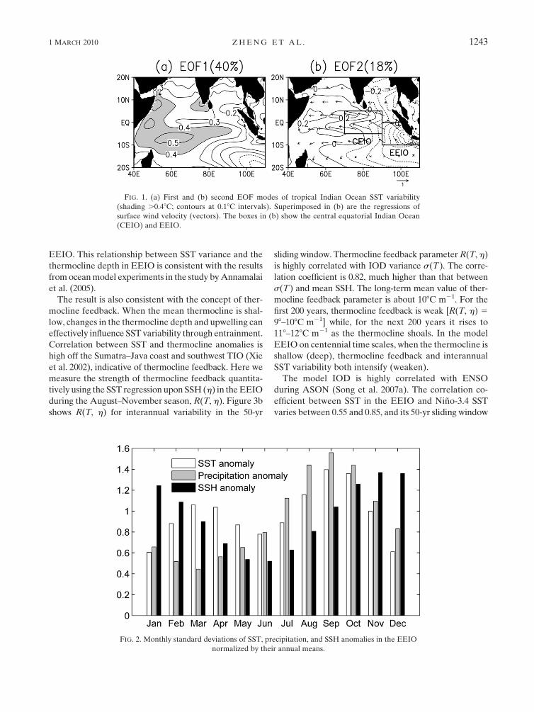
have performed an empirical orthogonal function anal-

ysis, and Fig. 1 shows the leading modes of interannual

SST variability over the TIO based on the 500-yr-long

control run1 with the CO2 level of year 1860. The first

EOF mode, explaining 40% of SST variance, exhibits a

basinwide warming. Previous studies (Klein et al. 1999;

Du et al. 2009) reported that this mode is a result of

ENSO forcing. Its correlation with the Nino-3.4 SST

index peaks when the basin mode lags by 4 months in the

model. The enhanced warming in the southwest TIO is

due to ocean Rossby wave propagation over the ther-

mocline ridge (Xie et al. 2002). The second EOF mode,

explaining 18% of SST variance, exhibits an east–west

dipole pattern with easterly wind anomalies along the

equator. The maximum negative SST anomalies are

located along the Java–Sumatra coasts where the wind-

forced upwelling occurs during June–October. The EOF

results are similar to those of Song et al. (2007a) and

comparable with observations.

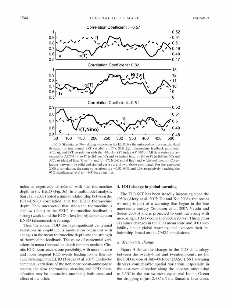
In addition to the spatial patterns, the model cap-

tures the IOD seasonality quite well. Figure 2 shows

monthly standard deviations of SST, precipitation, and

sea surface height (SSH) in the EEIO (108S-08, 908–

1108E), all displaying pronounced seasonality. SST

and precipitation variances are strong from August to

October, one month earlier than in observations. The

peak of SSH variance lags by 2–3 months in November–

December, a time delay due to equatorial wave propa-

gation (Yuan and Han 2006). In this paper, we use the

standard deviation of SST variability in the EEIO av-

eraged during August–October [ASON; s(T)] to rep-

resent IOD intensity. EEIO SST variability during

ASON is strongly affected by ocean upwelling and

thermocline feedback. EEIO SST and the Saji et al IOD

index based on the east 2 west SST difference are highly

correlated (r 5 0.96). The use of the latter index yields

the same results.

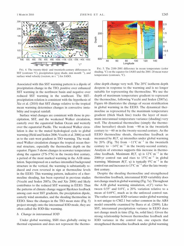
Figure 3a shows s(T) in 50-yr sliding windows. Cen-

tennial modulation is obvious: s(T) is about 0.658C in

the first 200 years and then rises above 0.88C from year

200 to 400. Overall s(T) varies between 0.68 and 0.98C,

a variation of 20% relative to the mean of 0.758C. Here

s(T) is correlated at 20.57 with sea surface height av-

eraged in sliding windows, which is taken as a proxy of

the thermocline depth in EEIO. The frequency of IOD

occurrence is also negatively correlated with time-mean

SSH (not shown), increasing as the thermocline shoals in

1 We have also examined an extended, 2000-yr-long control run,

and all the results reported in this section remain qualitatively the

same.

1242 J O U R N A L O F C L I M A T E VOLUME 23

EEIO. This relationship between SST variance and the

thermocline depth in EEIO is consistent with the results

from ocean model experiments in the study by Annamalai

et al. (2005).

The result is also consistent with the concept of ther-

mocline feedback. When the mean thermocline is shal-

low, changes in the thermocline depth and upwelling can

effectively influence SST variability through entrainment.

Correlation between SST and thermocline anomalies is

high off the Sumatra–Java coast and southwest TIO (Xie

et al. 2002), indicative of thermocline feedback. Here we

measure the strength of thermocline feedback quantita-

tively using the SST regression upon SSH (h) in the EEIO

during the August–November season, R(T, h). Figure 3b

shows R(T, h) for interannual variability in the 50-yr

sliding window. Thermocline feedback parameter R(T, h)

is highly correlated with IOD variance s(T). The corre-

lation coefficient is 0.82, much higher than that between

s(T) and mean SSH. The long-term mean value of ther-

mocline feedback parameter is about 108C m21. For the

first 200 years, thermocline feedback is weak [R(T, h) 5

98–108C m21] while, for the next 200 years it rises to

118–128C m21 as the thermocline shoals. In the model

EEIO on centennial time scales, when the thermocline is

shallow (deep), thermocline feedback and interannual

SST variability both intensify (weaken).

The model IOD is highly correlated with ENSO

during ASON (Song et al. 2007a). The correlation co-

efficient between SST in the EEIO and Nino-3.4 SST

varies between 0.55 and 0.85, and its 50-yr sliding window

FIG. 1. (a) First and (b) second EOF modes of tropical Indian Ocean SST variability

(shading .0.48C; contours at 0.18C intervals). Superimposed in (b) are the regressions of

surface wind velocity (vectors). The boxes in (b) show the central equatorial Indian Ocean

(CEIO) and EEIO.

FIG. 2. Monthly standard deviations of SST, precipitation, and SSH anomalies in the EEIO

normalized by their annual means.

1 MARCH 2010 Z H E N G E T A L . 1243

index is negatively correlated with the thermocline

depth in the EEIO (Fig. 3c). In a multimodel analysis,

Saji et al. (2006) noted a similar relationship between the

IOD–ENSO correlation and the EEIO thermocline

depth. They interpreted that, when the thermocline is

shallow (deep) in the EEIO, thermocline feedback is

strong (weak), and the IOD is less (more) dependent on

ENSO teleconnective forcing.

Thus the model IOD displays significant centennial

variations in amplitude, a modulation consistent with

changes in the mean thermocline depth and the strength

of thermocline feedback. The cause of centennial vari-

ations in mean thermocline depth remains unclear. Cha-

otic IOD occurrence is one possibility, with more intense

and more frequent IOD events leading to the thermo-

cline shoaling in the EEIO (Tozuka et al. 2007). In chaotic

centennial variations of the nonlinear ocean–atmosphere

system, the slow thermocline shoaling and IOD inten-

sification may be interactive, one being both cause and

effect of the other.

4. IOD change in global warming

The TIO SST has been steadily increasing since the

1950s (Alory et al. 2007; Du and Xie 2008); the recent

warming is part of a warming that began in the late

nineteenth century (Solomon et al. 2007; Vecchi and

Soden 2007b) and is projected to continue rising with

increasing GHG (Vecchi and Soden 2007a). This section

examines changes in the TIO mean state and IOD var-

iability under global warming and explores their re-

lationship, based on the CM2.1 simulations.

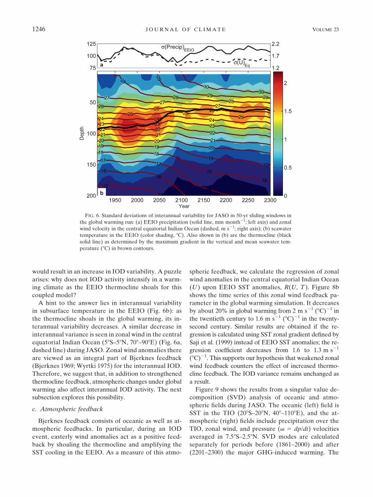
a. Mean state change

Figure 4 shows the change in the TIO climatology

between the twenty-third and twentieth centuries for

the IOD season of July–October (JASO). SST warming

displays considerable spatial variations, especially in

the east–west direction along the equator, amounting

to 3.68C in the northwestern equatorial Indian Ocean

but dropping to just 2.48C off the Sumatra–Java coast.

FIG. 3. Statistics in 50-yr sliding windows in the EEIO for the unforced control run: standard

deviation of interannual SST variability s(T ), SSH (h), thermocline feedback parameter

R(T, h), and SST correlation with the Nino-3.4 SST index r(T, Nino). All time series are av-

eraged for ASON: (a) s(T ) (solid line, 8C) and h (dashed line, m); (b) s(T ) (solid line, 8C) and

R(T, h) (dashed line, 8C m21); and (c) r(T, Nino) (solid line) and h (dashed line, m). Corre-

lations between the solid and dashed curves are shown above each panel. For the extended

2000-yr simulation, the same correlations are 20.32, 0.68, and 0.38, respectively, reaching the

95% significance level (r 5 0.3) based on t test.

1244 J O U R N A L O F C L I M A T E VOLUME 23

Associated with this SST warming pattern is a dipole of

precipitation change in the TIO, positive over enhanced

SST warming in the northwest basin and negative over

reduced SST warming in the southeast. The SST–

precipitation relation is consistent with the hypothesis of

Xie et al. (2010) that SST change relative to the tropical

mean warming determines changes in convective insta-

bility and tropical rainfall.

Surface wind changes are consistent with those in pre-

cipitation, SST, and the weakened Walker circulation,

easterly over the equatorial Indian Ocean and westerly

over the equatorial Pacific. The weakened Walker circu-

lation is due to the muted hydrological cycle to global

warming (Held and Soden 2006; Vecchi et al. 2006) as well

as to the east–west gradient in TIO warming. The weak-

ened Walker circulation changes the tropical ocean ther-

mal structure, especially the thermocline depth on the

equator. Figure 5 shows changes in seawater temperature

along the equator (58S–58N) in the twenty-first century,

a period of the most marked warming in the A1B simu-

lation. Superimposed on a surface-intensified background

structure in the vertical, the warming is substantially re-

duced and even reversed in sign at thermocline levels

in the EEIO. This warming pattern, indicative of a ther-

mocline shoaling, has been reported in previous studies

(Vecchi and Soden 2007a; Du and Xie 2008) and likely

contributes to the reduced SST warming in EEIO. Thus

the patterns of climate change suggest Bjerknes feedback

among east–west SST gradients, the precipitation dipole,

easterly wind anomalies, and the shoaling thermocline in

EEIO. Since the changes in the TIO mean state (Fig. 5)

project strongly onto the interannual IOD mode, they are

often called the IOD-like warming.

b. Change in interannual IOD

Under global warming, SSH rises globally owing to

thermal expansion and does not represent the thermo-

cline depth change very well. The 208C isotherm depth

deepens in response to the warming and is no longer

suitable for representing the thermocline. We use the

depth of maximum temperature gradient to represent

the thermocline, following Vecchi and Soden (2007a).

Figure 6b illustrates the change of ocean stratification

in global warming in the EEIO. The dynamical ther-

mocline as represented by the maximum temperature

gradient (thick black line) tracks the layer of maxi-

mum interannual temperature variance (shading) very

well. The dynamical thermocline (simply the thermo-

cline hereafter) shoals from ;90 m in the twentieth

century to ;60 m in the twenty-second century. As the

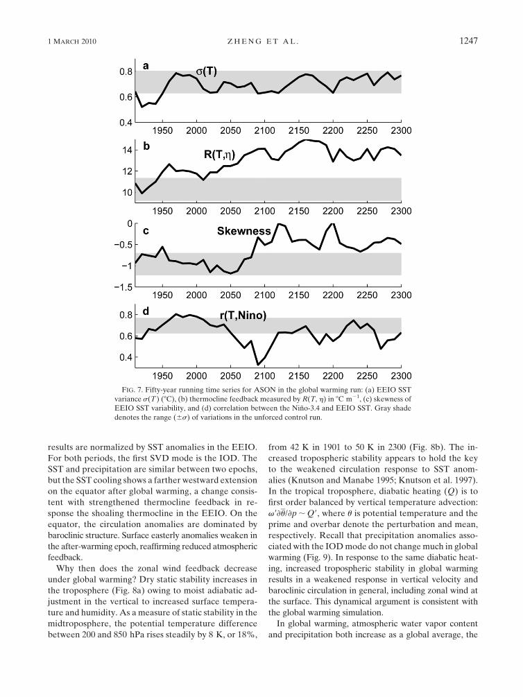
EEIO thermocline shoals, thermocline feedback as

measured by R(T, h) intensifies under global warming

by 20% (Fig. 7b) from ;118C m21 in the twentieth

century to ;148C m21 in the twenty-second century.

Analysis of extremes supports this increase in thermo-

cline feedback. Maximum R(T, h) is 128C m21 in the

2000-yr control run and rises to 158C m21 in global

warming. Minimum R(T, h) is typically 98C m21 in the

control run and increases to 138C m21 after the late twenty-

first century.

Despite the shoaling thermocline and strengthened

thermocline feedback, interannual IOD variability does

not change much in global warming (Fig. 7a). Throughout

the A1B global warming simulation, s(T) varies be-

tween 0.558 and 0.88C, a 20% variation relative to a

mean of 0.698C, much as in the unforced control run.

The rather constant IOD variance under global warming

is not unique to CM2.1 but rather common in the AR4

model ensemble examined by Ihara et al. (2009). Like

SST, interannual precipitation variance in EEIO does

not change much in time (Fig. 6a, solid line). Given the

strong relationship between thermocline feedback and

IOD variance in the control run, one expects that

strengthened thermocline feedback under global warming

FIG. 4. The twenty-third- and twentieth-century differences in

SST (contours 8C), precipitation (gray shade, mm month21), and

surface wind velocity (vectors, m s21) for JASO.

FIG. 5. The 2100–2001 difference in ocean temperature (color

shading, 8C) on the equator for JASO and the 2001–20 mean water

temperature (contours, 8C).

1 MARCH 2010 Z H E N G E T A L . 1245

would result in an increase in IOD variability. A puzzle

arises: why does not IOD activity intensify in a warm-

ing climate as the EEIO thermocline shoals for this

coupled model?

A hint to the answer lies in interannual variability

in subsurface temperature in the EEIO (Fig. 6b): as

the thermocline shoals in the global warming, its in-

terannual variability decreases. A similar decrease in

interannual variance is seen in zonal wind in the central

equatorial Indian Ocean (58S–58N, 708–908E) (Fig. 6a,

dashed line) during JASO. Zonal wind anomalies there

are viewed as an integral part of Bjerknes feedback

(Bjerknes 1969; Wyrtki 1975) for the interannual IOD.

Therefore, we suggest that, in addition to strengthened

thermocline feedback, atmospheric changes under global

warming also affect interannual IOD activity. The next

subsection explores this possibility.

c. Atmospheric feedback

Bjerknes feedback consists of oceanic as well as at-

mospheric feedbacks. In particular, during an IOD

event, easterly wind anomalies act as a positive feed-

back by shoaling the thermocline and amplifying the

SST cooling in the EEIO. As a measure of this atmo-

spheric feedback, we calculate the regression of zonal

wind anomalies in the central equatorial Indian Ocean

(U ) upon EEIO SST anomalies, R(U, T ). Figure 8b

shows the time series of this zonal wind feedback pa-

rameter in the global warming simulation. It decreases

by about 20% in global warming from 2 m s21 (8C)21 in

the twentieth century to 1.6 m s21 (8C)21 in the twenty-

second century. Similar results are obtained if the re-

gression is calculated using SST zonal gradient defined by

Saji et al. (1999) instead of EEIO SST anomalies; the re-

gression coefficient decreases from 1.6 to 1.3 m s21

(8C)21. This supports our hypothesis that weakened zonal

wind feedback counters the effect of increased thermo-

cline feedback. The IOD variance remains unchanged as

a result.

Figure 9 shows the results from a singular value de-

composition (SVD) analysis of oceanic and atmo-

spheric fields during JASO. The oceanic (left) field is

SST in the TIO (208S–208N, 408–1108E), and the at-

mospheric (right) fields include precipitation over the

TIO, zonal wind, and pressure (v 5 dp/dt) velocities

averaged in 7.58S–2.58N. SVD modes are calculated

separately for periods before (1861–2000) and after

(2201–2300) the major GHG-induced warming. The

FIG. 6. Standard deviations of interannual variability for JASO in 50-yr sliding windows in

the global warming run: (a) EEIO precipitation (solid line, mm month21; left axis) and zonal

wind velocity in the central equatorial Indian Ocean (dashed, m s21; right axis); (b) seawater

temperature in the EEIO (color shading, 8C). Also shown in (b) are the thermocline (black

solid line) as determined by the maximum gradient in the vertical and mean seawater tem-

perature (8C) in brown contours.

1246 J O U R N A L O F C L I M A T E VOLUME 23

results are normalized by SST anomalies in the EEIO.

For both periods, the first SVD mode is the IOD. The

SST and precipitation are similar between two epochs,

but the SST cooling shows a farther westward extension

on the equator after global warming, a change consis-

tent with strengthened thermocline feedback in re-

sponse the shoaling thermocline in the EEIO. On the

equator, the circulation anomalies are dominated by

baroclinic structure. Surface easterly anomalies weaken in

the after-warming epoch, reaffirming reduced atmospheric

feedback.

Why then does the zonal wind feedback decrease

under global warming? Dry static stability increases in

the troposphere (Fig. 8a) owing to moist adiabatic ad-

justment in the vertical to increased surface tempera-

ture and humidity. As a measure of static stability in the

midtroposphere, the potential temperature difference

between 200 and 850 hPa rises steadily by 8 K, or 18%,

from 42 K in 1901 to 50 K in 2300 (Fig. 8b). The in-

creased tropospheric stability appears to hold the key

to the weakened circulation response to SST anom-

alies (Knutson and Manabe 1995; Knutson et al. 1997).

In the tropical troposphere, diabatic heating (Q) is to

first order balanced by vertical temperature advection:

v9›u/›p ; Q9, where u is potential temperature and the

prime and overbar denote the perturbation and mean,

respectively. Recall that precipitation anomalies asso-

ciated with the IOD mode do not change much in global

warming (Fig. 9). In response to the same diabatic heat-

ing, increased tropospheric stability in global warming

results in a weakened response in vertical velocity and

baroclinic circulation in general, including zonal wind at

the surface. This dynamical argument is consistent with

the global warming simulation.

In global warming, atmospheric water vapor content

and precipitation both increase as a global average, the

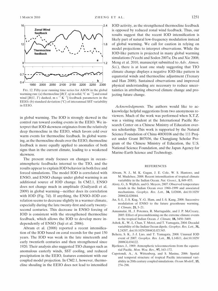
FIG. 7. Fifty-year running time series for ASON in the global warming run: (a) EEIO SST

variance s(T ) (8C), (b) thermocline feedback measured by R(T, h) in 8C m21, (c) skewness of

EEIO SST variability, and (d) correlation between the Nino-3.4 and EEIO SST. Gray shade

denotes the range (6s) of variations in the unforced control run.

1 MARCH 2010 Z H E N G E T A L . 1247

former following the Clausius–Clapeyron equation (Held

and Soden 2006; Vecchi and Soden 2007a; Richter and

Xie 2008). On regional scales, precipitation may increase

or decrease in global warming. Over the tropical Indian

Ocean, specifically, precipitation increases (decreases)

in the northwestern (southeastern) basin (Fig. 4). The

basin mean is nearly unchanged. As a result, precip-

itation response to IOD remains constant (Fig. 6a), and

FIG. 8. (a) Twenty-third minus twentieth-century difference in potential temperature (K)

averaged in the EEIO for JASO in the global warming run as a function of pressure (hPa);

(b) 50-yr running time series of �uj200 hPa850 hPa (dashed line, K) and zonal wind feedback parameter

R(U, T ) (solid line, m s21 K21) for JASO.

FIG. 9. First SVD mode between SST (color shading in bottom panel, 8C) and atmospheric

fields including precipitation (contours in bottom, mm month21) over the TIO, zonal (shading

in top, m s21) and vertical velocities (in Pa s21, vectors with zonal velocity) averaged in

58S–58N for ASON during (left) 1861–2000 and (right) 2201–2300.

1248 J O U R N A L O F C L I M A T E VOLUME 23

the tropospheric stability effect dominates atmospheric

feedback change.

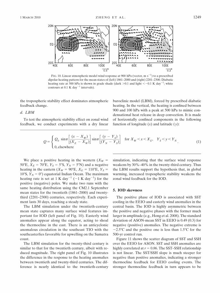
d. LBM

To test the atmospheric stability effect on zonal wind

feedback, we conduct experiments with a dry linear

baroclinic model (LBM), forced by prescribed diabatic

heating. In the vertical, the heating is confined between

900 and 100 hPa with a peak at 500 hPa to mimic con-

densational heat release in deep convection. It is made

of horizontally confined components in the following

function of longitude (x) and latitude (y):

Q 5Q

0sinp

(x � XW

)

(XE� X

W)

� �sinp

(y � YS)

(YN� Y

S)

� �for X

W, x , X

E, Y

S, y , Y

N

0, elsewhere

8<: . (1)

We place a positive heating in the western (XW 5

508E, XE 5 708E, YS 5 58S, YN 5 58N) and a negative

heating in the eastern (XW 5 908E, XE 5 1108E, YS 5

108S, YN 5 08) equatorial Indian Ocean. The maximum

heating rate is set at 1 K day21 (21 K day21) for the

positive (negative) poles. We make two runs with the

same heating distribution using the CM2.1 September

mean states for the twentieth (1861–2000) and twenty-

third (2201–2300) centuries, respectively. Each experi-

ment lasts 30 days, reaching a steady state.

The LBM simulation under the twentieth-century

mean state captures many surface wind features im-

portant for IOD (left panel of Fig. 10). Easterly wind

anomalies appear along the equator, acting to shoal

the thermocline in the east. There is an anticyclonic

anomalous circulation in the southeast TIO with the

southeasterlies favorable for upwelling on the Sumatra

coast.

The LBM simulation for the twenty-third century is

similar to that for the twentieth century, albeit with re-

duced magnitude. The right panel of Fig. 10 illustrates

the difference in the response to the heating anomalies

between twentieth and twenty-third centuries. The dif-

ference is nearly identical to the twentieth-century

simulation, indicating that the surface wind response

weakens by 30%–40% in the twenty-third century. Thus

the LBM results support the hypothesis that, in global

warming, increased tropospheric stability weakens the

zonal wind feedback for the IOD.

5. IOD skewness

The positive phase of IOD is associated with SST

cooling in the EEIO and easterly wind anomalies in the

central basin. The IOD is highly asymmetric between

the positive and negative phases with the former much

larger in amplitude (e.g., Hong et al. 2008). The standard

deviation of ASON-mean SST in EEIO is 0.49 (0.3) for

negative (positive) anomalies. The negative extreme is

22.58C and the positive one is less than 1.58C for the

500-yr control run.

Figure 11 shows the scatter diagram of SST and SSH

over the EEIO for ASON. SST and SSH anomalies are

highly correlated at r 5 0.86. The SST–SSH relationship

is not linear. The SST/SSH slope is much steeper for

negative than positive anomalies, indicating a stronger

thermocline feedback for EEIO cooling events. The

stronger thermocline feedback in turn appears to be

FIG. 10. Linear atmospheric model wind response at 900 hPa (vector, m s21) to a prescribed

dipolar heating pattern for the mean states of (left) 1861–2000 and (right) 2201–2300. Diabatic

heating rate at 500 hPa is shown in grade shade (dark .0.1 and light ,20.1 K day21; white

contours at 0.1 K day21 intervals).

1 MARCH 2010 Z H E N G E T A L . 1249

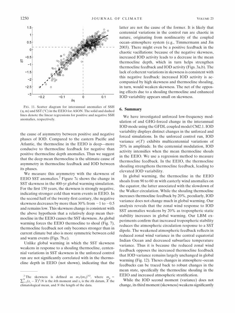
the cause of asymmetry between positive and negative

phases of IOD. Compared to the eastern Pacific and

Atlantic, the thermocline in the EEIO is deep—more

conducive to thermocline feedback for negative than

positive thermocline depth anomalies. Thus we suggest

that the deep mean thermocline is the ultimate cause of

asymmetry in thermocline feedback and IOD between

its phases.

We measure this asymmetry with the skewness of

EEIO SST anomalies.2 Figure 7c shows the change in

SST skewness in the 400-yr global warming simulation.

For the first 150 years, the skewness is strongly negative,

indicating stronger cold than warm events in EEIO. In

the second half of the twenty-first century, the negative

skewness decreases by more than 30% from 21 to 20.5

and remains low. This skewness change is consistent with

the above hypothesis that a relatively deep mean ther-

mocline in the EEIO causes the SST skewness. As global

warming forces the EEIO thermocline to shoal (Fig. 7),

thermocline feedback not only becomes stronger than in

current climate but also is more symmetric between cold

and warm events (Figs. 7b,c).

Unlike global warming in which the SST skewness

weakens in response to a shoaling thermocline, centen-

nial variations in SST skewness in the unforced control

run are not significantly correlated with in the thermo-

cline depth in EEIO (not shown), indicating that the

latter are not the cause of the former. It is likely that

centennial variations in the control run are chaotic in

nature, originating from nonlinearity of the coupled

ocean–atmosphere system (e.g., Timmermann and Jin

2003). There might even be a positive feedback in the

chaotic vacillations: because of the negative skewness,

increased IOD activity leads to a decrease in the mean

thermocline depth, which in turn helps strengthen

thermocline feedback and IOD activity (Figs. 3a,b). The

lack of coherent variations in skewness is consistent with

this negative feedback: increased IOD activity is ac-

companied by high skewness and thermocline shoaling,

in turn, would weaken skewness. The net of the oppos-

ing effects due to a shoaling thermocline and enhanced

IOD variability appears small on skewness.

6. Summary

We have investigated unforced low-frequency mod-

ulation of and GHG-forced change in the interannual

IOD mode using the GFDL coupled model CM2.1. IOD

variability displays distinct changes in the unforced and

forced simulations. In the unforced control run, IOD

variance s(T) exhibits multicentennial variations of

20% in amplitude. In the centennial modulation, IOD

activity intensifies when the mean thermocline shoals

in the EEIO. We use a regression method to measure

thermocline feedback. In the EEIO, the thermocline

shoaling strengthens thermocline feedback, leading to

elevated IOD variability.

In global warming, the thermocline in the EEIO

shoals from 90 to 60 m with easterly wind anomalies on

the equator, the latter associated with the slowdown of

the Walker circulation. While the shoaling thermocline

increases thermocline feedback by 20%, peculiarly, IOD

variance does not change much in global warming. Our

analysis reveals that the zonal wind response to IOD

SST anomalies weakens by 20% as tropospheric static

stability increases in global warming. Our LBM ex-

periments confirm that increased tropospheric stability

reduces the atmospheric circulation response to a SST

dipole. The weakened atmospheric feedback reflects in

reduced zonal wind variance in the central equatorial

Indian Ocean and decreased subsurface temperature

variance. Thus it is because the reduced zonal wind

feedback opposes the increased thermocline feedback

that IOD variance remains largely unchanged in global

warming (Fig. 12). Theses changes in atmosphere–ocean

feedbacks can be traced back to robust changes in the

mean state, specifically the thermocline shoaling in the

EEIO and increased atmospheric stratification.

While the IOD second moment (variance) does not

change, its third moment (skewness) weakens significantly

FIG. 11. Scatter diagram for interannual anomalies of SSH

(h, m) and SST (8C) in the EEIO for ASON. The solid and dashed

lines denote the linear regressions for positive and negative SSH

anomalies, respectively.

2 The skewness is defined as m3/(m2)3/2, where mk

5

�N

i51(xi�X)k/N is the kth moment and xi is the ith datum, X the

climatological mean, and N the length of the data.

1250 J O U R N A L O F C L I M A T E VOLUME 23

in global warming. The IOD is strongly skewed in the

control run toward cooling events in the EEIO. We in-

terpret that IOD skewness originates from the relatively

deep thermocline in the EEIO, which favors cold over

warm events for thermocline feedback. In global warm-

ing, as the thermocline shoals over the EEIO, thermocline

feedback is more equally applied to anomalies of both

signs than in the current climate, leading to a weakened

skewness.

The present study focuses on changes in ocean–

atmospheric feedbacks internal to the TIO, and the

results appear to explain IOD behavior in both free and

forced simulations. The model IOD is correlated with

ENSO, and ENSO change under global warming is an

additional source of IOD change. In CM2.1, ENSO

does not change much in amplitude (Guilyardi et al.

2009) in global warming—neither does its correlation

with IOD (Fig. 7d). If anything, the ENSO–IOD cor-

relation seems to decrease slightly in a warmer climate,

especially during the late twenty-first and early twenty-

second centuries. This decrease in ENSO forcing of

IOD is consistent with the strengthened thermocline

feedback, which allows the IOD to develop more in-

dependently of ENSO (Saji et al. 2006).

Abram et al. (2008) reported a recent intensifica-

tion of the IOD based on coral records for the past 150

years. The IOD was weak in the late nineteenth and

early twentieth centuries and then strengthened since

1920. Their analysis also suggested TIO changes such as

anomalous easterly winds, SST cooling, and reduced

precipitation in the EEIO, features consistent with our

coupled model projection. In CM2.1, however, thermo-

cline shoaling in the EEIO does not lead to intensified

IOD activity, as the strengthened thermocline feedback

is opposed by reduced zonal wind feedback. Thus, our

results suggest that the recent IOD intensification is

likely part of natural low-frequency modulation instead

of global warming. We call for caution in relying on

model projections to interpret observations. While the

IOD-like pattern is projected in many global warming

simulations (Vecchi and Soden 2007a; Du and Xie 2008;

Meng et al. 2010, manuscript submitted to Adv. Atmos.

Sci.), there is at least one study suggesting that TIO

climate change displays a negative IOD-like pattern in

equatorial winds and thermocline adjustment (Trenary

and Han 2008). Sustained observations and improved

physical understanding are necessary to reduce uncer-

tainties in attributing observed climate change and pro-

jecting future change.

Acknowledgments. The authors would like to ac-

knowledge helpful suggestions from two anonymous re-

viewers. Much of the work was performed when X.T.Z.

was a visiting student at the International Pacific Re-

search Center on a Chinese Ministry of Education over-

sea scholarship. This work is supported by the Natural

Science Foundation of China 40830106 and the 111 Proj-

ect under Grant B07036, the Changjiang Scholar Pro-

gram of the Chinese Ministry of Education, the U.S.

National Science Foundation, and the Japan Agency for

Marine-Earth Science and Technology.

REFERENCES

Abram, N. J., M. K. Gagan, J. E. Cole, W. S. Hantoro, and

M. Mudelsee, 2008: Recent intensification of tropical climate

variability in the Indian Ocean. Nat. Geosci., 1, 849–853.

Alory, G., S. Wijffels, and G. Meyers, 2007: Observed temperature

trends in the Indian Ocean over 1960–1999 and associated

mechanisms. Geophys. Res. Lett., 34, L02606, doi:10.1029/

2006GL028044.

An, S.-I., J.-S. Kug, Y.-G. Ham, and I.-S. Kang, 2008: Successive

modulation of ENSO to the future greenhouse warming.

J. Climate, 21, 3–21.

Annamalai, H., J. Potemra, R. Murtugudde, and J. P. McCreary,

2005: Effect of preconditioning on the extreme climate events

in the tropical Indian Ocean. J. Climate, 18, 3450–3469.

Ashok, K., W.-L. Chan, T. Motoi, and T. Yamagata, 2004: Decadal

variability of the Indian Ocean dipole. Geophys. Res. Lett., 31,

L24207, doi:10.1029/2004GL021345.

Behera, S. K., J.-J. Luo, and T. Yamagata, 2008: Unusual IOD

event of 2007. Geophys. Res. Lett., 35, L14S11, doi:10.1029/

2008GL034122.

Bjerknes, J., 1969: Atmospheric teleconnections from the equato-

rial Pacific. Mon. Wea. Rev., 97, 163–172.

Capotondi, A., A. Wittenberg, and S. Masina, 2006: Spatial

and temporal structure of tropical Pacific interannual vari-

ability in 20th century coupled simulations. Ocean Modell., 15,

274–298.

FIG. 12. Fifty-year running time series for ASON in the global

warming run: (a) thermocline [R(T, h) in solid, 8C m21] and zonal

wind [R(U, T ) dashed, m s21 K21] feedback parameters in the

EEIO; (b) standard deviation (8C) of interannual SST variability

in EEIO.

1 MARCH 2010 Z H E N G E T A L . 1251

Chang, P., and Coauthors, 2006: Climate fluctuations of tropical

coupled system—The role of ocean dynamics. J. Climate, 19,

5122–5174.

Collins, M., 2005: El Nino- or La Nina-like climate change? Climate

Dyn., 24, 89–104.

Delworth, T. L., and Coauthors, 2006: GFDL’s CM2 global coupled

climate models. Part I: Formulation and simulation character-

istics. J. Climate, 19, 643–674.

Deser, C., A. S. Phillips, and J. W. Hurrell, 2004: Pacific inter-

decadal climate variability: Linkages between the tropics and

the North Pacific during boreal winter since 1900. J. Climate,

17, 3109–3124.

Du, Y., and S.-P. Xie, 2008: Role of atmospheric adjustments in the

tropical Indian Ocean warming during the 20th century in

climate models. Geophys. Res. Lett., 35, L08712, doi:10.1029/

2008GL033631.

——, ——, G. Huang, and K. Hu, 2009: Role of air–sea interaction

in the long persistence of El Nino–induced north Indian Ocean

warming. J. Climate, 22, 2023–2038.

Fedorov, A. V., and S. G. Philander, 2000: Is El Nino changing?

Science, 288, 1997–2002.

GFDL Global Atmospheric Model Development Team, 2004:

The new GFDL global atmosphere and land model AM2–

LM2: Evaluation with prescribed SST simulations. J. Cli-

mate, 17, 4641–4673.

Griffies, S., M. J. Harrison, R. C. Pacanowski, and A. Rosati,

2003: A technical guide to MOM4. GFDL Ocean Group

Tech. Rep. 5, NOAA/Geophysical Fluid Dynamics Labora-

tory, 295 pp.

Guilyardi, E., A. Wittenberg, A. Fedorov, M. Collins, C. Wang,

A. Capotondi, G. J. van Oldenborgh, and T. Stockdale, 2009:

Understanding El Nino in ocean–atmosphere general circu-

lation models: Progress and challenges. Bull. Amer. Meteor.

Soc., 90, 325–340.

Held, I. M., and B. J. Soden, 2006: Robust responses of the hy-

drological cycle to global warming. J. Climate, 19, 5686–

5699.

Hong, C.-C., T. Li, LinHo, and J.-S. Kug, 2008: Asymmetry of the

Indian Ocean dipole. Part I: Observational analysis. J. Cli-

mate, 21, 4834–4848.

Ihara, C., Y. Kushnir, and M. A. Cane, 2008: Warming trend of the

Indian Ocean SST and Indian Ocean dipole from 1880 to 2004.

J. Climate, 21, 2035–2046.

——, ——, ——, and H. P. Victor, 2009: Climate change over

the equatorial Indo-Pacific in global warming. J. Climate, 22,

2678–2693.

Klein, S. A., B. J. Soden, and N.-C. Lau, 1999: Remote sea surface

temperature variations during ENSO: Evidence for a tropical

atmospheric bridge. J. Climate, 12, 917–932.

Knutson, T. R., and S. Manabe, 1995: Time-mean response over

the tropical Pacific to increased CO2 in a coupled ocean–

atmosphere model. J. Climate, 8, 2181–2199.

——, ——, and D. Gu, 1997: Simulated ENSO in a global

coupled ocean–atmosphere model: Multidecadal ampli-

tude modulation and CO2 sensitivity. J. Climate, 10, 138–

161.

Lin, S.-J., 2004: A ‘‘vertically Lagrangian’’ finite-volume dy-

namical core for global models. Mon. Wea. Rev., 132, 2293–

2307.

Luo, J. J., S. K. Behera, Y. Masumoto, H. Sakuma, and T. Yamagata,

2008: Successful prediction of the consecutive IOD in 2006

and 2007. Geophys. Res. Lett., 35, L14S02, doi:10.1029/

2007GL032793.

Meehl, G. A., G. W. Branstator, and W. M. Washington, 1993:

Tropical Pacific interannual variability and CO2 climate

change. J. Climate, 6, 42–63.

Murtugudde, R., J. P. McCreary, and A. J. Busalacchi, 2000:

Oceanic processes associated with anomalous events in the

Indian Ocean with relevance to 1997–1998. J. Geophys. Res.,

105, 3295–3306.

Richter, I., and S.-P. Xie, 2008: Muted precipitation increase in

global warming simulations: A surface evaporation perspective.

J. Geophys. Res., 113, D24118, doi:10.1029/2008JD010561.

Saji, N. H., B. N. Goswami, P. N. Vinayachandran, and T. Yamagata,

1999: A dipole mode in the tropical Indian Ocean. Nature, 401,

360–363.

——, S.-P. Xie, and T. Yamagata, 2006: Tropical Indian Ocean

variability in the IPCC twentieth-century climate simulations.

J. Climate, 19, 4397–4417.

Schott, F. A., S.-P. Xie, and J. P. McCreary, 2009: Indian Ocean

circulation and climate variability. Rev. Geophys., 47, RG1002,

doi:10.1029/2007RG000245.

Solomon, S., D. Qin, M. Manning, M. Marquis, K. Averyt,

M. M. B. Tignor, H. L. Miller Jr., and Z. Chen, Eds., 2007:

Climate Change 2007: The Physical Science Basis. Cambridge

University Press, 996 pp.

Song, Q. N., G. A. Vecchi, and A. Rosati, 2007a: Indian Ocean

variability in the GFDL CM2 coupled climate model. J. Cli-

mate, 20, 2895–2916.

——, ——, and ——, 2007b: The role of the Indonesian Through-

flow in the Indo–Pacific climate variability in the GFDL

Coupled Climate Model. J. Climate, 20, 2434–2451.

Timmermann, A., and F.-F. Jin, 2003: A nonlinear theory for

El Nino bursting. J. Atmos. Sci., 60, 152–165.

——, J. Oberhuber, A. Bacher, M. Esch, M. Latif, and E. Roeckner,

1999: Increased El Nino frequency in a climate model forced

by future greenhouse warming. Nature, 398, 694–697.

Tozuka, T., J. J. Luo, S. Masson, and T. Yamagata, 2007: Decadal

modulations of the Indian Ocean Dipole in the SINTEX-F1

coupled GCM. J. Climate, 20, 2881–2894.

Trenary, L. L., and W. Han, 2008: Causes of decadal subsurface

cooling in the tropical Indian Ocean during 1961–2000. Geo-

phys. Res. Lett., 35, L17602, doi:10.1029/2008GL034687.

van Oldenborgh, G. J., S. Philip, and M. Collins, 2005: El Nino

in a changing climate: A multi-model study. Ocean Sci., 1,

81–85.

Vecchi, G. A., and B. J. Soden, 2007a: Global warming and the

weakening of the tropical circulation. J. Climate, 20, 4316–

4340.

——, and ——, 2007b: Effect of remote sea surface temperature

change on tropical cyclone potential intensity. Nature, 450,

1066–1070.

——, ——, A. T. Wittenberg, I. M. Held, A. Leetmaa, and

M. J. Harrison, 2006: Weakening of tropical Pacific atmo-

spheric circulation due to anthropogenic forcing. Nature, 441,

73–76.

Watanabe, M., and M. Kimoto, 2000: Atmosphere-ocean thermal

coupling in the North Atlantic: A positive feedback. Quart.

J. Roy. Meteor. Soc., 126, 3343–3369.

Webster, P. J., A. M. Moore, J. P. Loschnigg, and R. R. Leben,

1999: Coupled ocean–atmosphere dynamics in the Indian

Ocean during 1997–98. Nature, 401, 356–360.

Wittenberg, A. T., A. Rosati, N.-C. Lau, and J. J. Ploshay, 2006:

GFDL’s CM2 global coupled climate models. Part III:

Tropical Pacific climate and ENSO. J. Climate, 19, 698–722.

1252 J O U R N A L O F C L I M A T E VOLUME 23

Wyrtki, K., 1975: El Nino—The dynamic response of the equatorial

Pacific Ocean to atmospheric forcing. J. Phys. Oceanogr., 5,

572–584.

Xie, S.-P., H. Annamalai, F. A. Schott, and J. P. McCreary, 2002:

Structure and mechanisms of south Indian Ocean climate

variability. J. Climate, 15, 864–878.

——, C. Deser, G. A. Vecchi, J. Ma, H. Teng, and A. T. Wittenberg,

2010: Global warming pattern formation: Sea surface temper-

ature and rainfall. J. Climate, 23, 966–986.

Yamagata, T., S. K. Behera, J.-J. Luo, S. Masson, M. Jury, and

S. A. Rao, 2004: Coupled ocean–atmosphere variability in the

tropical Indian Ocean. Earth Climate: The Ocean–Atmosphere

Interaction, Geophys. Monogr., Vol. 147, Amer. Geophys.

Union, 189–212.

Yuan, D., and W. Han, 2006: Roles of equatorial waves and

western boundary reflection in the seasonal circulation

of the equatorial Indian Ocean. J. Phys. Oceanogr., 36,930–944.

1 MARCH 2010 Z H E N G E T A L . 1253