Report No. 22171-IN INDIA POWER SUPPLY TO AGRICULTURE VOLUME 2 HARYANA CASE STUDY June 15, 2001 Energy Sector Unit South Asia Regional Office

Document of the World Bank

CONTENTS

Page No. CHAPTER 1 THE IMPORTANCE OF ELECTRICITY TO THE AGRICULTURE

SECTOR IN HARYANA A. Introduction .................................................................................................................................1 B. Methodology ...............................................................................................................................3 C. Characteristics of the Sampled Farmers .....................................................................................5

CHAPTER 2 CONSUMPTION OF POWER BY AGRICULTURE: MYTHS AND REALITIES

A. Introduction ...............................................................................................................................12 B. Electricity Sales to Agriculture Sector ......................................................................................12 C. Assessment of Realistic Levels of Electricity Consumption by Agriculture Sector .................13 D. Comparison of Study Results with Haryana Estimates .............................................................16 E. Actual Connected Load by Farmers ..........................................................................................18 F. Availability and Reliability of Power Supply to Agriculture.....................................................18 G. The Scope for End Use Efficiency Improvement......................................................................23 H. Metering Agriculture Consumers ..............................................................................................24

CHAPTER 3 HOW IRRIGATION TECHNOLOGY CHOICES AFFECT FARM INCOMES A. Introduction ...............................................................................................................................26 B. Gross Farm Income ...................................................................................................................26 C. Production Costs .......................................................................................................................27 D. Decomposition of Irrigation Costs ............................................................................................30 E. Variable Costs for Rice and Wheat Across Technologies .........................................................33 F. Costs of Poor Quality of Supply in Operation of Electric Pumps..............................................34 G. Transformer Burn Outs .............................................................................................................35 H. Per Unit Tariff Paid by farmers (including cost due to poor Quality).......................................37 I. Net farm income Across Farm Sizes...........................................................................................38 J. Non-Farm Sources of Income.....................................................................................................39

CHAPTER 4 DETERMINANTS OF CHOICE OF IRRIGATION TECHNOLOGY

AND FARM INCOMES A. Introduction ...............................................................................................................................41 B. Determinants of Technology Choices .......................................................................................41 C. Technology Choice Determinants .............................................................................................43 D. Determinants of Total Pump Capacity (HP) .............................................................................43 E. Diesel Pump as a Coping Strategy............................................................................................45 F. Investing in Diesel Pump by Non-Electric Pump Owners........................................................45 G. Net Farm income Determinants.................................................................................................46 H. Determinants of Short Run Electricity Consumption................................................................47 I. Policy Simulations ....................................................................................................................48 J. The Effects of Tariff Reforms and Electricity Supply Improvements on net farm income.......50

K. Returns from Improvements in Reliability and Quality of Power Supply: Comparison of Electric and Diesel Pumps .......................................................................53

CHAPTER 5 CONCLUSIONS AND RECOMMENDATIONS A. Introduction ...............................................................................................................................55 B. Metering Agriculture Consumers ..............................................................................................55 C. Tariff Structure .........................................................................................................................56 D. Raising Electricity Tariffs .........................................................................................................56 E. Canal Water Pricing...................................................................................................................57 F. Complementary Measures to Improve Returns to Agricultural Production Activities ..............57 G. Integrated Approaches to Energy Efficiency ............................................................................59

TABLES Table 1.1 Sample Distribution of all farmers in recall survey by regions .................................................4 Table 1.2 Average land owned (hectares)..................................................................................................6 Table 1.3 Average gross area cultivated annually (hectares).....................................................................7 Table 1.4 Average horsepower per unit of gross cultivated area by farm .................................................8 Table 2.1 Haryana: Electricity Consumption by Agriculture Sector .......................................................13 Table 2.2 FY2000 Sample results-Average consumption per pump (kWh/pump)..................................14 Table 2.3 Extrapolation of sample results: Electricity consumption by Agriculture Sector in Haryana ............................................................................................................15 Table 2.4 Comparison of study results with HVPN (FY99-2000) Total electricity sales (GWh) ...........16 Table 2.5 Comparison of study results with HVPN (FY99-2000) (kWh/kW) ........................................17 Table 2.6 Assessment of T&D losses in Haryana....................................................................................17 Table 2.7 Cost Recovery of Electricity Supply to Agriculture Sector.....................................................18 Table 2.8 Availability of Power in Haryana ............................................................................................20 Table 2.9 Availability and Reliability for four feeders of Haryana .........................................................21 Table 2.10 Energy savings from implementing comprehensive pumpset replace program ......................24 Table 2.11 Summary of types of benefits in Integrated Agricultural DSM Program................................24 Table 3.1 Average annual gross income by farm size (Rs) .....................................................................27 Table 3.2 Gross farm income per hectare of net cultivated area (Rs./Ha) ...............................................27 Table 3.3 Production Cost as percent of gross income............................................................................29 Table 3.4 Electricity tariffs for agricultural sector in Haryana in FY2000..............................................30 Table 3.5 Variable irrigation costs for Kharif paddy cultivation by farm size category in Haryana (Rs/Ha)..........................................................................................................33 Table 3.6 Variable irrigation costs per hectare for wheat in Haryana .....................................................34 Table 3.7 Frequency distribution of rewindings per pump by season .....................................................35 Table 3.8 Frequency of transformer burn-outs and time taken for rectification in Haryana ...................36 Table 3.9 Annual net farm income per farm............................................................................................38 Table 3.10 Net farm income per net cultivated area (Rs/ha) .....................................................................39 Table 3.11 Distribution of average non-farm income................................................................................40 Table 4.1 Short-term willingness to pay for improvement in different power supply indicators ............49 Table 4.2 Medium-term willingness to pay for improvement in different power supply indicators .......49 Table 4.3 Rates of tariff increase which would leave farmers no worse off in short-run........................50 Table 4.4 Medium term effect of policy scenarios I, II and III................................................................51 Table 4.5 Policy scenario I – No reform scenario ...................................................................................51 Table 4.6 Policy scenario II - Delayed reform scenario with aggressive tariff increase .........................52 Table 4.7 Policy scenario III - Delayed reform scenario with gradual tariff increase .............................52 Table 4.8 Policy scenario II – Accelerated reform scenario ....................................................................53

FIGURES Figure 1.1 Size Distribution of different sample categories of farmers (land owned) ................................6 Figure 1.2 Average horsepower of pumpsets by region and groundwater depth........................................9 Figure 1.3 Main reasons given for using diesel pump ..............................................................................10 Figure 1.4 Problems faced in getting electricity connection.....................................................................10 Figure 1.5 Terms on which non-electric diesel farmers would use electric pumpsets..............................11 Figure 2.2 The Range of supply voltage received at pumpsets.................................................................22 Figure 3.1 Electric pumps only: Irrigation cost as a percent of gross farm income..................................31 Figure 3.2 Electric with canal: Irrigation cost as a percent of gross farm income ....................................32 Figure 3.3 Electric with diesel pumps: Irrigation cost as a percent of gross farm income .......................32 Figure 3.4 Transformer burnout in Haryana ............................................................................................36 Figure 3.5 Percentage of farmers reporting non-farm income ..................................................................39 ANNEXES Annex 1: The Agriculture Sector in Haryana: An Overview .......................................................................... Annex 2: Characteristics of the Sample Farmers ............................................................................................ Annex 3: Metering Study Results ................................................................................................................... Annex 4: Methodology for Tariff Cost Computation...................................................................................... Annex 5: Statistical Tables.............................................................................................................................. Annex 6: Determinants of Choice of irrigation Technology and Farm Income.............................................. Annex 7: Economic Benefits of Metering…………………………………………………………………... Annex 8: Haryana's comments on the Report……………………………………………………………….

CHAPTER 1

THE IMPORTANCE OF ELECTRICITY TO THE AGRICULTURE SECTOR IN HARYANA

A. Introduction

1.1 The supply of electric power to agricultural consumers is often regarded as the root of the crisis of the power sector in India. The tariffs charged to agriculture (agricultural tariffs) are estimated to represent a fraction of the increasing cost of power supply, and some states like Tamil Nadu and Punjab supply power to agricultural consumers free of charge. In Haryana farmers pay just 12 per cent of the cost of supply yet they use nearly half of the electricity produced, according to the Haryana State Electricity Board (HSEB 1999). Obviously the decision to increase tariffs is among the measures that generate the strongest political opposition. Therefore, the urgent need for structural and policy reforms in the power sector has brought to the forefront the need to disentangle more clearly the interdependent relationship between the agricultural and power sectors. 1.2 The agricultural sector is key to the economic development of the state of Haryana. In FY1998, agriculture contributed to a 36 per cent share of the Gross State Domestic Product (GSDP) and employed 60 per cent of the workforce of the State. Over 70 per cent of the State’s population reside in the rural areas (CMIE 1999a); where in FY1994, 80 per cent of the poor lived (World Bank 1998). Continued agricultural growth is therefore viewed to be critical not only in sustaining Haryana’s economic growth, but also in reducing poverty, as it drives rural employment and income growth. Haryana’s agricultural performance also has important implications on the overall food security of the country. Haryana is one of the major surplus producers of basic staples, specifically rice and wheat: while accounting for only 1 per cent of the land area in India, it produces about 7 per cent of the rice and wheat in the country (CMIE 1999b). See Annex 1 for an overview of the Haryana agriculture sector. 1.3 The improvements in agriculture production have come primarily due to the expansion of irrigated agriculture. In FY1996 seventy seven per cent of the total net cropped area was irrigated, up 23 per cent from 1982. Irrigation has also led to an increase in cropping intensity. Of the area irrigated nearly half was irrigated using water supplied via pumps and the rest via canals. Canals cover close to three quarters of Haryana but only farmers closest to the canals can use the water efficiently and most farmers who use canal water supplement its use by pumping groundwater. In Haryana more farmers own electric pumps than diesel pumps and more than 40 per cent of diesel pump owners said that they would use electric pumps if they could get a connection. 1.4 The power sector, therefore, exerts a critical influence on the performance of the agricultural sector as it affects farmer access to and use of power for a variety of agricultural operations, but most importantly for pumping groundwater for irrigation purposes. This presents another area of concern. In the long term, the increased use of groundwater, a scarce resource in an arid state like Haryana, will eventually have negative effects on agricultural production. Tariff reform coupled with improvements in electricity supply will also ensure a better management of scarce groundwater resources for the future health of agricultural production in Haryana. 1.5 This study has been done in collaboration with the government of Haryana to assess the impact of power policy reforms on agriculture. It demonstrates how reforms of the electricity tariff structure, combined with an improvement in the quality of power supply can help maintain productivity gains in agriculture and increase farmers' incomes. At the same time, it will ensure a commercially viable power

-2-

sector. For the first time these results are based on solid empirical data collected through surveys of farmers and actual metering on the supply and use of power by farmers. 1.6 Based on an econometric model, developed to analyze data collection, three scenarios have been formulated to simulate the impact of different policies. The bottom line is clear: small and marginal farmers, who make up 40 per cent (Fig 1.1) of sampled farmers with electric pumpsets in Haryana, will suffer most if there are no reforms, whereas all farmers are expected to see improvements in their incomes with gradual adjustment of tariffs and a simultaneous improvement in service. At present it is the marginal and small farmers who are most adversely affected by the regressive nature of the current flat rate pricing for electricity. 1.7 What follows in this chapter is a resume of the methodology of the analysis undertaken, the profile of the farmers surveyed and their irrigation choices. A separate report describes in detail the methodology and sampling. This chapter shows that farmers who use electricity for pumping (either on its own or in conjunction with other sources of irrigation) cultivate more land than farmers who do not use electricity for irrigation and that farmers with electric pumps have the highest cropping intensity. As is shown in a subsequent chapter, the amount of land under cultivation and cropping patterns have a direct positive impact on farm incomes. 1.8 Chapter Two discusses the ways farmers use electricity, what is the impact of its availability and what is the impact of the reliability of that availability. It makes two conclusions: (i) farmers use less electricity than the utility attributes to them which means that part of the subsidies to agriculture goes in reality to finance theft of electricity, and (ii) the utility does not supply electricity when it says it would and the quality of supply is poor, consequently farmers spend significantly on coping strategies (i.e. extra pumps and higher horse powered pumps) and on repairs to equipment. 1.9 Chapter Three discusses the relationship between irrigation choices and farm incomes. It describes the regressive nature of the current flat rate tariff and shows the costs associated with the different irrigation choices. It also shows that farmers who use electric pumps have the highest incomes. In general farmers who use electric pumps have gross incomes five times that of farmers who purchase water or rely solely on rainfall. For marginal farmers, electric pump users have incomes three times higher than farmers that buy in water or rely solely on rainfall.

1.10 Chapter Four looks at the determinants for technology choices and their impact on farm incomes. The econometric model developed for this study from the primary data collected via metering and surveys is the first attempt to analyse the different parameters related to the condition of power supply on farm production and income. Chapter Five presents the main conclusions and recommendations.

-3-

B. Methodology

1.11 A partial equilibrium analysis is adopted to evaluate the impact of power policy reforms on agriculture. The focus is to examine the impact of policy reforms on the cost of production and on farm incomes for different categories of consumers (see The Report on Methodological Framework and Sampling Procedures). 1.12 The study examines how electricity supply conditions (availability, reliability, quality etc.) affect technology choices, farm incomes and electricity demand, controlling for other factors. Existing conditions of electricity supply affect farmers in several ways. Econometric anaylsis is, therefore, used to investigate the determinants of farmers' incomes as a result of irrigation technology choices. Over the long run, farmers are likely to choose the irrigation technology that maximizes the expected discounted

Map of Haryana

by Districts

-4-

value of future returns subject to the constraints that they face. Once these technology decisions are made, during any given season farmers choose: (i) how much land to cultivate (analysed through the net farm income in the econometric model); (ii) how much variable inputs (including electricity) to apply (analysed through the electricity consumption function in the econometric model). All these input and output choices, in turn, determine farm incomes in each season. 1.13 Collection of primary data consisted of (a) metering sample farm pump sets, and (b) metering a sample of rural feeders to monitor and evaluate the quality of power supply, and (c) conducting an Attitude and six Recall surveys of farmers. The sample and the sampling procedures were discussed and agreed with Haryana utilities. In November 1998, energy meters were installed on 600 pumpsets in Haryana. Staff of the Haryana Vidyut Prasaran Nigam Limited, HVPNL (HVPNL - the Haryana electricity utility) recorded the metered consumption every fortnight up to July 2000. A total of 1,659 farmers from the five different regions were surveyed (Table 1.1). A consulting firm conducted: (a) an attitude survey to assess the views of farmers on the supply of power to agriculture, (b) two recall surveys in each of the three cropping seasons in Haryana: Rabi season (December-April 1999-2000), Summer season (June-July 1999), and Kharif season (August-November 1999). These recall surveys covered a full-one year agriculture cycle. The recall surveys covered farmers using all irrigation technologies, such as rain, canal irrigation, diesel and electricity pump sets and water markets.

Table 1.1 - Sample distribution of all farmers in recall survey by regions

Pump owners Non-pump owners

Region Electric pump

owners

Non-electric diesel pump

owners

Canal users

Water purchasers Rainfed

Total

I 83 24 0 30 15 152 II 307 32 25 40 23 427 III 126 94 53 73 54 400 IV 191 36 18 87 26 358 V 70 63 155 15 19 322 Overall 777 249 251 245 137 1,659

Notes: This table includes only those sample farmers for whom complete land and cultivation data is available Source: Farmers’ recall data

1.14 Both the metering as well as the recall surveys were conducted on a sample of farmers from five different regions (See Map of Haryana). The regions were selected to ensure farming conditions, such as cropping patterns, types of irrigation used, rainfall and water quality, were similar within a region as compared to those in other regions1. Farmers were classified into several categories according to irrigation choices and the amount of land they owned and/or cultivated. Since the primary focus of this study is on farmers who own electric pumps, for this category a larger sample was chosen2. For the other categories, 883 farmers were surveyed, including 249 non-electric diesel pump owners, 251 non-pump canal users and 245 non-pump water purchasers. The sample also included 137 rainfed farmers.

1.15 The sample category of electric pump owners is defined as those farmers who have electric pumps. Some of these farmers may also have diesel pumps and/or use canal water. Similarly, the sample category of diesel pump owners is defined as those farmers who do not own electric pumps, but own diesel pumps. Some of these farmers may also use canal water in conjunction with pumps.

1 See Methodology Framework and Sampling Procedures, Table H-1 2 Sampling of farmers was done through a 2-stage stratified random sampling procedure, with regions as strata, group of villages served by a selected feeder as primary sampling unit (PSU) and farmers as defined above in the selected groups of villages, as secondary sampling units (SSUs). Villages served by selected feeders were completely enumerated and farmers classified according to irrigation status so as to generate lists of SSU's under each category of farmers for each selected feeder. From this list, the ratio of farmers under each sample category to total number of farmers was obtained for each region. Since the primary focus of this study is on farmers who own electric pumps, this category was over-sampled.

-5-

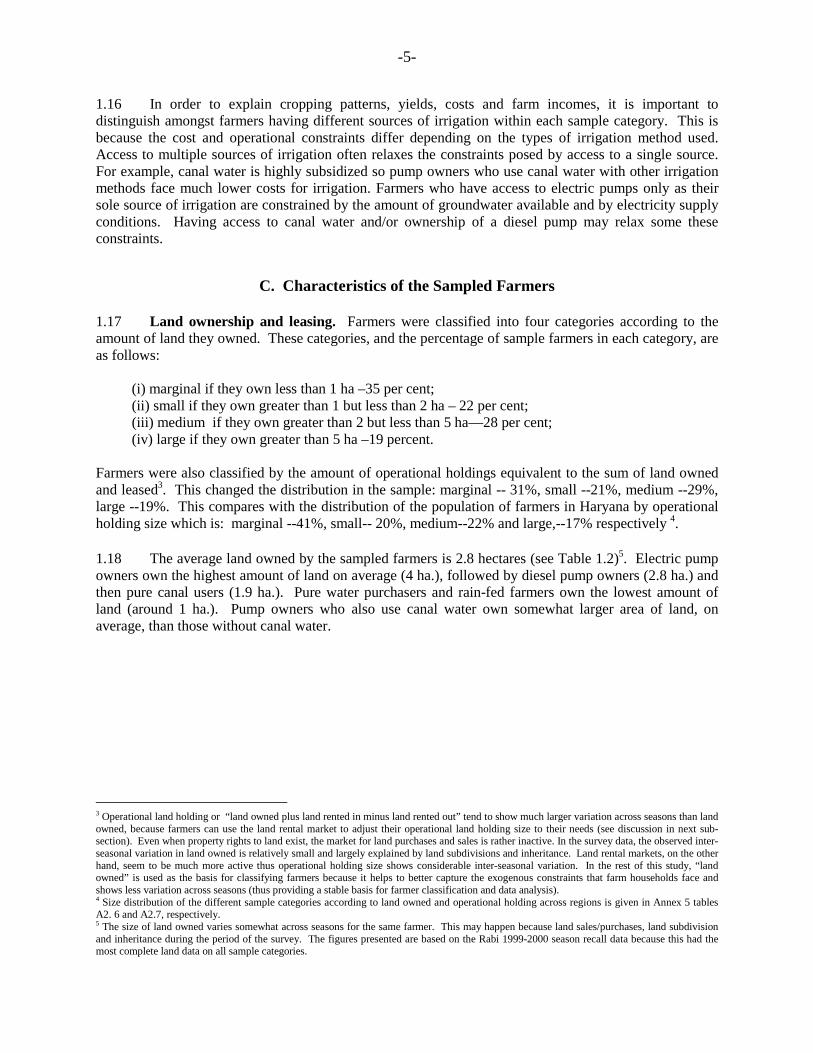
1.16 In order to explain cropping patterns, yields, costs and farm incomes, it is important to distinguish amongst farmers having different sources of irrigation within each sample category. This is because the cost and operational constraints differ depending on the types of irrigation method used. Access to multiple sources of irrigation often relaxes the constraints posed by access to a single source. For example, canal water is highly subsidized so pump owners who use canal water with other irrigation methods face much lower costs for irrigation. Farmers who have access to electric pumps only as their sole source of irrigation are constrained by the amount of groundwater available and by electricity supply conditions. Having access to canal water and/or ownership of a diesel pump may relax some these constraints.

C. Characteristics of the Sampled Farmers

1.17 Land ownership and leasing. Farmers were classified into four categories according to the amount of land they owned. These categories, and the percentage of sample farmers in each category, are as follows:

(i) marginal if they own less than 1 ha –35 per cent; (ii) small if they own greater than 1 but less than 2 ha – 22 per cent; (iii) medium if they own greater than 2 but less than 5 ha—28 per cent; (iv) large if they own greater than 5 ha –19 percent.

Farmers were also classified by the amount of operational holdings equivalent to the sum of land owned and leased3. This changed the distribution in the sample: marginal -- 31%, small --21%, medium --29%, large --19%. This compares with the distribution of the population of farmers in Haryana by operational holding size which is: marginal --41%, small-- 20%, medium--22% and large,--17% respectively 4. 1.18 The average land owned by the sampled farmers is 2.8 hectares (see Table 1.2)5. Electric pump owners own the highest amount of land on average (4 ha.), followed by diesel pump owners (2.8 ha.) and then pure canal users (1.9 ha.). Pure water purchasers and rain-fed farmers own the lowest amount of land (around 1 ha.). Pump owners who also use canal water own somewhat larger area of land, on average, than those without canal water.

3 Operational land holding or “land owned plus land rented in minus land rented out” tend to show much larger variation across seasons than land owned, because farmers can use the land rental market to adjust their operational land holding size to their needs (see discussion in next sub-section). Even when property rights to land exist, the market for land purchases and sales is rather inactive. In the survey data, the observed inter-seasonal variation in land owned is relatively small and largely explained by land subdivisions and inheritance. Land rental markets, on the other hand, seem to be much more active thus operational holding size shows considerable inter-seasonal variation. In the rest of this study, “land owned” is used as the basis for classifying farmers because it helps to better capture the exogenous constraints that farm households face and shows less variation across seasons (thus providing a stable basis for farmer classification and data analysis). 4 Size distribution of the different sample categories according to land owned and operational holding across regions is given in Annex 5 tables A2. 6 and A2.7, respectively. 5 The size of land owned varies somewhat across seasons for the same farmer. This may happen because land sales/purchases, land subdivision and inheritance during the period of the survey. The figures presented are based on the Rabi 1999-2000 season recall data because this had the most complete land data on all sample categories.

-6-

Table 1.2 - Average land owned (hectares)

Electric pump owners Non-electric diesel pump owners Farm size Category Electric

only

Electric and

canal

Electric and

diesel Total Diesel

only Diesel and

canal Total

Non-pump Canal Users

Non-pump Water

purchasers Rainfed Total

Marginal 0.5 0.7 0.5 0.5 0.6 0.6 0.6 0.5 0.5 0.5 0.5 Small 1.5 1.2 1.3 1.4 1.3 1.3 1.3 1.4 1.3 1.4 1.4 Medium 3.1 3.2 3.2 3.1 3.0 3.3 3.1 3.0 2.5 2.9 3.1 Large 9.6 11.8 10.3 10.1 7.2 9.6 8.7 7.8 7.0 7.9 9.7 Overall 3.4 5.9 4.7 4.0 2.2 4.4 2.8 1.9 1.0 1.1 2.8 Source: Rabi 99-00 recall data

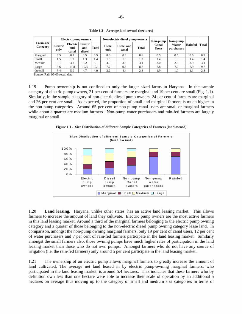
1.19 Pump ownership is not confined to only the larger sized farms in Haryana. In the sample category of electric pump owners, 21 per cent of farmers are marginal and 19 per cent are small (Fig. 1.1). Similarly, in the sample category of non-electric diesel pump owners, 24 per cent of farmers are marginal and 26 per cent are small. As expected, the proportion of small and marginal farmers is much higher in the non-pump categories. Around 65 per cent of non-pump canal users are small or marginal farmers while about a quarter are medium farmers. Non-pump water purchasers and rain-fed farmers are largely marginal or small.

Figure 1.1 - Size Distribution of different Sample Categories of Farmers (land owned)

1.20 Land leasing. Haryana, unlike other states, has an active land leasing market. This allows farmers to increase the amount of land they cultivate. Electric pump owners are the most active farmers in this land leasing market. Around a third of the marginal farmers belonging to the electric pump owning category and a quarter of those belonging to the non-electric diesel pump owning category lease land. In comparison, amongst the non-pump owning marginal farmers, only 19 per cent of canal users, 12 per cent of water purchasers and 7 per cent of rain-fed farmers participate in the land leasing market. Similarly amongst the small farmers also, those owning pumps have much higher rates of participation in the land leasing market than those who do not own pumps. Amongst farmers who do not have any source of irrigation (i.e. the rain-fed farmers) only around 5 per cent participate in the land leasing market. 1.21 The ownership of an electric pump allows marginal farmers to greatly increase the amount of land cultivated. The average net land leased in by electric pump-owning marginal farmers, who participated in the land leasing market, is around 5.4 hectares. This indicates that these farmers who by definition own less than one hectare were able to increase their scale of operation by an additional 5 hectares on average thus moving up to the category of small and medium size categories in terms of

S iz e D istr ib u tio n o f d i ffe re n t S a m p le C a te g o ri e s o f F a rm e rs (l a n d o w n e d )

0 %2 0 %4 0 %6 0 %8 0 %

1 0 0 %

E le c tr icp u m p

o wn e r s

D ie s e lp u m p

o wn e r s

No n p u m pC a n a l

o wn e r s

No n - p u m pwa te r

p u r c h a s e r s

R a in fe d

M a r g in a l S m a ll M e d iu m L a r g e

-7-

operational holding. In contrast, marginal farmers who do not own any pumps not only participate less in the land leasing market but also amongst those who do participate the net land leased in is much smaller (around 0.6 ha. for water purchasers and rain-fed). This shows that unlike their electric pump owning counterparts, these marginal farmers are less able to expand their operational holding through the land leasing market. The net leased in land by marginal farmers who own electric pumps is much higher than those who do not own electric pumps but own diesel pumps. 1.22 Gross cultivated area and cropping intensity. Farms with electric pumpsets are able to cultivate more acreage and more intensively than farms using other irrigation technology. In particular, marginal farmers with electric pumps were able to cultivate more than double the acreage of non-electric pump owners and six times that of marginal rain-fed farmers. In addition, the gross area cultivated by farmers who use electric pumps in conjunction with canal water cultivate double the amount of land than farmers who rely solely on electric pumps. Average gross cultivated area per farm, that is the sum of the area cultivated in the different seasons, is 5.7 hectares across the sample (Table 1.3). The average gross area cultivated by electric pump owners is 8.9 hectares. Within that category, the non pump water purchasers and rainfed farmers have the lowest gross area under cultivation. In the non-electric diesel pump category, the gross cultivated area by farmers who use diesel pumps in conjunction with canal water is more than double that for farmers who use diesel pumps alone. Use of multiple sources of irrigation clearly allows for a larger gross area under cultivation.

Table 1.3 - Average gross area cultivated annually (hectares)

Electric pump owners Non-electric diesel pump owners Region/

farm size category Electric

only

Electric and

canal

Electric and

diesel Total Diesel

only

Diesel and

canal Total

Non-pump Canal users

Non-pump Water

purchasers Rainfed Total

Marginal 2.4 3.8 3 2.9 1.3 1.7 1.6 1.5 1.1 0.5 1.5 Small 3.4 7 5.2 4 2.8 3 3 2.9 2.7 1 3.2 Medium 7.5 8 8.4 7.9 5 5.9 5.3 5.8 4.3 2.6 6.7 Large 17.5 22.8 20.7 19 8.5 14.9 12.1 7.4 6.9 2 16.6 Overall 7.4 14.8 10.9 8.9 3.7 7.7 4.9 3.6 1.9 0.9 5.7 Source: Farmers’ recall data

1.23 Farmers who own electric pumps have the highest cropping intensity, while rain-fed farmers have the lowest cropping intensity, i.e. cultivating the same land over different growing seasons. Farmers who own diesel pumps only, have the lowest cropping intensity amongst farmers who use some source of irrigation. Farmers who depend solely on purchased water as their source of irrigation have higher cropping intensities on average than farmers in all other categories except the electric pump owning farmers. Cropping intensity is about 200 per cent in all regions (Annex 5 table A2.18).

1.24 Cropping Patterns. By season, the major crops in the State are: in the Kharif season, rice and cotton, accounting respectively for 72 per cent and 24 per cent of cropped area; in the Rabi season, wheat, accounting for 86 per cent of cropped area; and in the Summer season, jowar and bajra accounting for 52 per cent and 30 per cent respectively of cropped area. The availability of water throughout the different growing seasons and the prevalence of pumps affects cropping decisions. For example, as rice is a water intensive crop, the proportion of irrigated area devoted to rice is inversely related to the relative costs of the water available. In areas where canal water (the cheapest source) is used for irrigation, 100 per cent of the area is cultivated with paddy, except in Region V. Electric pump users are able to irrigate 90 per cent of the rice area compared to diesel pump users who managed to cultivate between 40 per cent and 90 per cent of their rice area. Cropping patterns are detailed in Annex 5, tables A2.19-20. It appears a contradiction that in an arid state such as Haryana, and in particular in areas where the water table is decreasing, farmers can grow water intensive crops.

-8-

1.25 Pump ownership. The picture of pump ownership as observed by the sample across Haryana is complex. Around 47 per cent of farmers own more than one electric pump and some farmers may have complete or partial ownership in several pumps. There are several reasons why this might be so such as the need to deal with fragmented plots, inheritance, opportunities for joint ownership with other farms and the need for back up or coping strategies in response to poor quality electricity. As one would expect, marginal and small farmers own fewer pumps than medium and large farmers but some do own more than one. Around 18 per cent of marginal farmers who own electric pumps own more than one, whereas around 71 per cent of large farmers owned more than one electric pump.

Table 1.4 - Average Horsepower per Unit of Gross Cultivated area by Farm (HP/gross cultivated hectare)

Farm size categories Region Pump Type Marginal Small Medium Large All

Diesel 3.8 1.8 0.3 0.1 0.8 I Electric 1.4 0.6 0.9 0.7 0.9 Diesel 1 0.7 0.2 0 0.6 II Electric 1.2 1 0.6 0.4 0.9 Diesel 4.1 2.1 1.3 0.7 1.9 III Electric 0.7 0.3 0.4 0.4 0.5 Diesel 1 0.7 0.3 0.1 0.5 IV Electric 2.5 0.9 0.8 0.8 1.1 Diesel 3.8 1.6 1.2 0.4 1 V Electric 0.2 0.8 0.5 0.4 0.5 Diesel 1.8 1.1 0.7 0.3 0.9 All Electric 1.4 0.8 0.6 0.6 0.8

Source: Farmers’ recall data 1.26 Small farmers tend to invest in higher HP pumps than their farm size might warrant. (see Table 1.4). The reason for owning more than one pump and pumps of a higher HP is linked to the quality of the electricity supply in Haryana in addition to other factors. Farmers invest in extra pumping capacity, be it a larger pump or a second pump, in order to cope with the erratic pattern of power supply in the state. 1.27 Number and type of pumps owned. The sample farmers owned a total of 988 pumps 6. These included 670 electric pumps (of which 589 were metered as part of the metering study) and 318 diesel pumps. Electric and diesel pump ownership is not confined to only larger farmers. Of the 670 electric pumps in the sample, around a quarter are owned by small or marginal farmers. Furthermore, of the 217 diesel pumps that are owned by farmers who do not have electric pumps, close to half (around 52 per cent) are owned by small or marginal farmers. In addition, small and marginal farmers account for 11 per cent of the diesel pumps that are owned jointly with electric pumps7. 1.28 Distribution of pump horsepower (HP) reported by farmers8. The average size of electric pump motors in the sample is around 7 HP while that for diesel pumps is around 8 HP (Figure 1.3). There is considerable variation in pump size (as measured by pump HP) across regions. It seems to show some correlation with groundwater depth and farm size, as expected. In later chapters, the role of different factors (such as electricity supply conditions, landholding size and groundwater depth) in influencing the choice of pump type and size is examined.

6 Sample farmers were asked about their ownership share in each of the pump(s) they own. If a farmer owned one pump exclusively and another pump jointly with others, with the farmer’s ownership share in the joint pump being half, then the number of pumps owned was taken as 1.5. 7 Those who own diesel pumps only, were asked about the reasons why they invested in diesel pumps as opposed to electric pumps. These reasons are discussed in the next sub-section. 8 In general there have been discrepancies observed between the actual horsepower of the pump see Chapter Two (see para2.6) and that reported by farmers. Unless otherwise noted, the HP cited in this report is that reported by the farmers.

-9-

Figure 1. 2- Average horsepower of pumpsets by region and groundwater depth, ft.

Note: Groundwater depth-average for the year. Source: Haryana well investment recall data for HP distribution. Farmers’ summer-99 season recall data for groundwater depths.

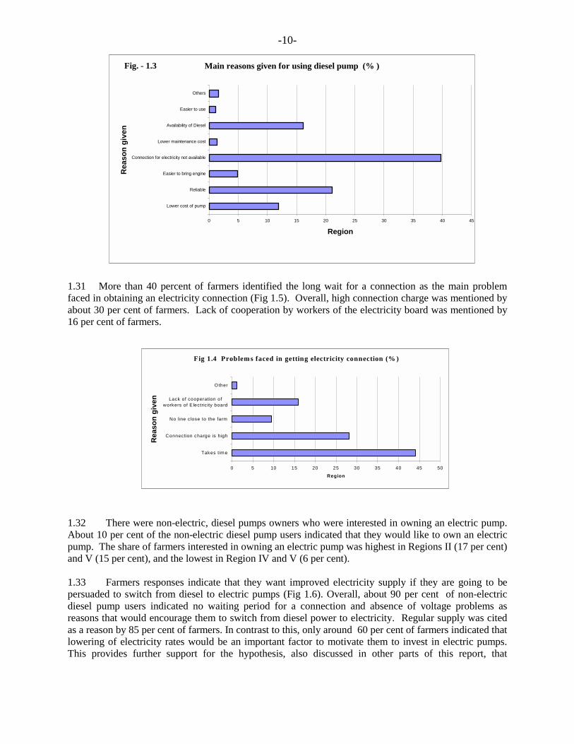
1.29 Although small and marginal farmers generally operate pumps with lower HP in absolute terms there appears to be an inverse relationship between farm size and the horsepower per hectare of gross cultivated area (see Table 1.7) 9. That is, smaller farmers tend to invest in higher HP per unit of gross cultivated area relative to larger farmers. There are several reasons for this. First, small and marginal farmers who tend to be more risk averse might be investing in high HP pumps to cope with the availability and uncertainty about power supply. In contrast to larger farmers who could invest in additional diesel pumps, smaller farmers are left to be more dependent purely on electric pumps. Second, given the minimum limited size of pumps available and the indivisibility in pump sizes available, farmers maybe compelled to purchase a larger pump than is economically justified by the area they are farming. Third, large HP pumps may be a necessity in regions where groundwater depth is very high, such as in Region V (see Fig. 1.3). 1.30 Farmer preferences for electric pumps versus diesel pumps. Diesel pump owning farmers who do not have electric pumps were asked why they had not invested in electric pumps. The biggest reason by far—cited by 40 per cent of farmers across all regions - was the unavailability of an electricity connection. This points to the large latent demand for electricity connections in rural Haryana (see Fig 1.4 below).

9 Gross cultivated area is defined as the sum of the area cultivated in the different seasons.

02468

10121416

I II III IV V Overall

Region

Hp

of p

ump

0

2040

60

80100

120

Gro

undw

ater

dep

th, f

t

Electric pumps Diesel pumpsGroundwater depth

-10-

1.31 More than 40 percent of farmers identified the long wait for a connection as the main problem faced in obtaining an electricity connection (Fig 1.5). Overall, high connection charge was mentioned by about 30 per cent of farmers. Lack of cooperation by workers of the electricity board was mentioned by 16 per cent of farmers.

1.32 There were non-electric, diesel pumps owners who were interested in owning an electric pump. About 10 per cent of the non-electric diesel pump users indicated that they would like to own an electric pump. The share of farmers interested in owning an electric pump was highest in Regions II (17 per cent) and V (15 per cent), and the lowest in Region IV and V (6 per cent). 1.33 Farmers responses indicate that they want improved electricity supply if they are going to be persuaded to switch from diesel to electric pumps (Fig 1.6). Overall, about 90 per cent of non-electric diesel pump users indicated no waiting period for a connection and absence of voltage problems as reasons that would encourage them to switch from diesel power to electricity. Regular supply was cited as a reason by 85 per cent of farmers. In contrast to this, only around 60 per cent of farmers indicated that lowering of electricity rates would be an important factor to motivate them to invest in electric pumps. This provides further support for the hypothesis, also discussed in other parts of this report, that

Fig 1.4 Problem s faced in getting electricity connection (% )

0 5 10 15 20 25 30 35 40 45 50

Takes tim e

Connection charge is high

No line c lose to the farm

Lack of cooperation ofworkers of E lectric ity board

O ther

Rea

son

give

n

Region

Main reasons given for using diesel pump (% )

0 5 10 15 20 25 30 35 40 45

Lower cost of pump

Reliable

Easier to bring engine

Connection for electricity not available

Lower maintenance cost

Availability of Diesel

Easier to use

Others

Rea

son

give

n

Region

Fig. - 1.3

-11-

improvements in quality and reliability of electricity are perceived by farmers to be of paramount importance. Around 56 per cent farmers also pointed to billing based on metered readings to be important.

Fig 1.5 - Terms on which non-electric diesel farmers would use electric pumpsets (%)

Note: Due to multiple responses percentages do not add up to 100. Source: Diesel farmers’ recall data

0 2 0 4 0 6 0 8 0 1 0 0

N o w a it in g p e rio d fo r C o n n e c tio n

N o V o lta g e p ro b le m s

R e g u la r su p p ly o f e le c tric ity

L o w e r co n n e c tio n ch a rg e s

L o w e r e le c tric ity ra te s

B ill b a se d o n m e te r

O th e r

-12-

CHAPTER 2

CONSUMPTION OF POWER BY AGRICULTURE: MYTHS AND REALITIES

A. Introduction 2.1 In India, the level of consumption of power by agriculture has been estimated by the utilities in the absence of systematic information and method. Because of the flat rate tariff structure and the lack of meters, there is no reliable estimate of how much electricity is used by farmers. This study uses a systematic collection of data from meters installed in a sample of pumpsets in Haryana that were chosen according to a rigorous statistical procedure. For the first time, therefore, the accuracy of the estimated electricity consumption by farmers in Haryana is based on a solid statistical method. The results show that farmers use less power than the utility estimates and that, therefore, transmission and distribution losses are higher than previously believed. A separate feeder study also demonstrates that farmers do not receive the amount of power promised by the utility and that the quality of power supply is poor and inconsistent.

B. Electricity Sales to Agriculture Sector 2.2 In Haryana, as in all other states in India10, electricity supply to agriculture consumers is mostly un-metered with a tariff based on the connected load (HP) of pumpsets. In the absence of metering, utilities just estimate the consumption by the agriculture sector. Usually, the amount of total electricity available for sale11 is allocated between sales to agriculture consumers and transmission and distribution losses, after aggregating the extent of metered sales to various categories of consumers. The tendency to under-estimate transmission and distribution (T&D) losses, in the absence of adequate system for accounting for flow of energy in the system, is widely apparent. A significant portion of non-technical loss, which essentially constitutes theft/ pilferage of electricity, is therefore camouflaged as consumption by the agriculture sector. 2.3 Official statistics show the growth rate in electricity consumption over the past thirty years does not correspond with the growth rate of either agricultural users, connected load or agricultural production. Table 2.1 shows the increase in electricity sales to the agriculture sector from 300 GWh in FY1971 to 950 GWh in FY1981 and to about 4,100 GWh in FY1999. This makes a compounded annual growth rate of about 10 per cent, compared to an overall growth rate of total sales of 8.4per cent. Accordingly the share of agriculture sector in the total electricity sales increased from 31 per cent in FY1971 to 46 per cent in FY1999, as per utility estimates.

10 During mid seventies to early eighties most of the State Electricity Boards in India shifted away from metering of electricity sales to agriculture consumers and introduced tariffs based on capacity of the pumps. This was undertaken apparently for administrative convenience and to minimize costs involved in metering, billing and collection of agriculture consumers scattered throughout the states in far and remote areas. Among the states who have high electricity consumption in the agriculture sector, Andhra Pradesh, Uttar Pradesh, Punjab, Tamil Nadu, and Karnataka do not meter any agriculture connections. Rajasthan is the only state which has about half of its agriculture connections metered, but they account for only one-fifth of the total electricity sales to agriculture consumers. Haryana, Maharasthra and Kerala also have some metered agriculture connections. 11 Total electricity available for sale for the utility is defined as the sum of generation (net of auxiliary consumption) from own power stations and power purchased from central generating stations, independent power producers (IPPs), and other utilities.

-13-

Table 2.1 - Haryana: Electricity Consumption by Agriculture Sector

FY1971 FY1981 FY1991 FY1996 FY1999 Growth Rate (%)

Total no. of consumers (’000) 544 1219 2514 3172 3381 6.7 Total no. of agriculture consumers (‘000) 86 226 345 376 359 5.2 % agriculture consumers 15.8 18.5 13.7 11.9 10.6 Total connected load (MW) 897 2358 4555 6193 6987 7.6 Connected load agriculture sector (MW) 389 1052 1618 2017 2045 6.1 % agriculture connected load 43.4 44.6 35.5 32.6 29.3 Total Sales (GWh) 939 2793 6134 8358 8900 8.4 Sales to Agriculture Sector (GWh) 299 954 2712 3094 4090 9.8 % sales to agriculture Sector 31.8 34.2 44.2 46.7 46.0 Specific electricity consumption per pump connection (kWh/pump) 3477 4221 7861 8229 11393

Specific consumption – kWh/kW 769 907 1676 1534 2000 Source: Haryana Vidyut Prasaran Nigam Ltd.

2.4 Haryana introduced the flat rate based tariff for agriculture consumers in 1978 and from that time there was a rapid growth rate in electricity consumption. But there is no similar trend in the growth rate of the number of consumers and connected load. The consumption trend was not mirrored in agricultural production. For example, the period FY1979 to FY 1998, the food grain production12 in Haryana increased at an annual growth rate of about 3 per cent, where as the utilities reported a growth rate of 8 per cent per annum in electricity consumption by the agriculture sector. During this period, the gross cropped area under food grain production remained more or less the same.

C. Assessment of Realistic Levels of Electricity Consumption by Agriculture Sector 2.5 The above analysis would lead one to assume that not all the power attributed by the utility to the agricultural sector is used by farmers. The on-farm metering of sample electric pump sets carried out for the FY2000 growing season quantified this assumption. Using the following analysis of data collected from a sample of electric pumps it is estimated that during FY2000 Haryana agriculture sector consumed 2,900 Gwh. The standard error of the estimate for total consumption, based on the sample, is equivalent to 12.5 per cent. 2.6 Sample Selection: The report on Methodology and Sampling details how electric pumps were selected and provides a more detailed look at the data collected. Following the subdivision into five agro-climatic zones, a total of 150 transformers were selected for metering and a sample of 600 pumpsets connected to the transformers were selected. 2.7 Meter Reading. The consumption pattern of the sample of 58413 electric pumps was monitored through installation of new meters. Even on pumps for which farmers have opted for metered tariffs and meters had been in place, new meters were installed for the study purpose. The meter readings were taken by the utility staff every fortnight starting from December 1998. The readings recorded by the utility staff were validated periodically by the consultants during their field visits as well as through regular review and check of the meter reading data sent by HVPN to identify possible obvious errors. The analysis of the meter readings of the sample presented here corresponds to one full year FY2000, covering three seasons - Summer, Kharif and Rabi, in order to understand and relate the pattern of electricity consumption to cropping pattern and agricultural activity in different seasons. 12 About two-third of the gross cropped area in Haryana is used for food grain cultivation. 13 Out of the total sample of 600 pumps, there were delays and problems in installation of meters on some pumps and therefore finally for the analysis under the study 584 pumps have been considered.

-14-

2.8 Results: Consumption per Pump. The electricity consumption estimates for the three seasons in the five regions is provided in Table 2.2. The average electricity consumption by pump set is estimated at about 8,150 kWh/pump. The recorded consumption is the highest during the Kharif season, which is agriculturally the most active season (this season corresponds with monsoon season) and with the water intensive crop paddy as the predominant crop; followed by the Rabi season with wheat as the main crop. Summer season (April to end June) is agriculturally not an active season (only about 56 per cent of the total farmers surveyed during this season were found to be cultivating, against 76 per cent in case of Kharif and 95 per cent in the case of Rabi season). The average operational holding 14 (this varies across season due to leasing in/out of land and differing amount of seasonal fallow left by the farmers) of the sample farmers also shows a corresponding trend, being estimated as the lowest in Summer at 3.5 ha, and the highest in Kharif and Rabi season at 4.5 ha.

Table 2.2 - FY2000 Sample Results – Average Consumption per Pump (kWh/pump) Regions Season

I II III IV V Total

Summer 3,123 1,500 736 1,490 3,540 1,855 Kharif 5,728 3,092 2,532 2,281 7,503 3,697 Rabi 3,392 1,251 1,289 3,764 5,100 2,622 Total FY2000 11,842 5,868 4,621 7,630 15,978 8,150

2.9 Hours of Pump Usage. To translate the above estimates of average consumption per pump across regions and seasons into hours of electric pump usage by farmers, the average connected load of the sample pumps (as reported by the utilities) is considered with respect to each of the regions. For the sample study, the average hours of operation by agriculture pumps is estimated to be 1,500 hours per annum or about 4 hours per day through out the year15. There are marked variations in the pump usage during different agricultural seasons; average hours of pump usage per day is estimated to be about 3.5 hours during the Summer and Rabi season and about 5 hours per day in the Kharif season. 2.10 Extrapolation of the Sample Results. The methodology of the aggregation for estimating average power consumption for each region is described in detail in the report on methodology and sampling. The meter readings of the sample pumps are used to estimate the average consumption per pump i.e. "kWh/pump"16. The average consumption per pump at the sample transformer level is based on the average kWh/pump of all the pumps attached to that transformer. The average consumption per pump at the feeder level is arrived based on weighted average consumption per pump of all the transformers (in the sample), the weight for each transformer defined as the proportion of pumps attached to that transformer to total pumps (in the sample at feeder level). Similarly, the average consumption per pump at the region level is arrived as the weighted average consumption per pump for each of the feeders in the sample. Finally the total electricity consumption in each of the regions is estimated as the product of

14 Operational holding is defined as land owned plus land leased in plus fallow land less land leased out less seasonal fallow. 15 This is the average hours of pump use per day on annual basis. During agriculturally active period during the year the farmers would tend to use pumps for much higher than 4 hours/day where as during non-active period they may not operate the pump at all. Thus it is important to note that even though the utility may be supplying power for 8 hours per day as per their supply regulation policy for agriculture sector, farmers would not run their pumps everyday for 8 hours and thus the average hours of usage for the year would be less . 16 For estimating electricity consumption by each pump, the fortnightly meter readings obtained from HVPN staff were reviewed carefully, to appropriately address the gaps in meter readings, if any. In case of a single gap in the meter reading, if prior / later readings are available, the missing reading is worked out by linear extrapolation. In case of multiple successive missing meter readings, the readings are extrapolated from the previous/later readings provided at least 50% of the readings are available for the particular season. In case some intermediate reading is smaller than its previous reading and shows gradual increase for next few fortnights, it is treated as a case of meter replacement, and the consumption for such a pump is obtained by aggregating the consumption figures for the sub-periods i.e. before and after the meter replacement. Any pump with missing readings not falling in these three categories is excluded from the estimation of electricity consumption. Accordingly, readings from 96%, 94% and 92% of the 584 sample meters installed under the study were considered for estimation of electricity consumption during summer, Kharif and Rabi season respectively.

-15-

average consumption per pump in each region (for Summer, Kharif and Rabi seasons) and the total number of electric pumps in the region17. 2.11 Based on the sample metering and the methodology summarized above, electricity consumption by agriculture sector in FY2000 is estimated at 2,900 GWh (see Table 2.3). Total electricity consumption in each region as well as for the state is estimated as the product of number of electric pumps and consumption per pump (kWh/pump). Regional differences are detailed in the methodology and sampling report. The standard error of the estimate for the total consumption is equivalent to 12.5 per cent.

Table 2.3 - Extrapolation of Sample Results: Electricity Consumption by

Agriculture Sector in Haryana (FY2000)

I II III IV V State No. of agriculture consumers 37,655 139,630 40,770 87,639 47,171 352,875

Consumption per pump (kWh) 11842 5868 4621 7630 15978 8150

Standard Error (%) 15.7% 10.6% 33.7% 24.6% 39.9% 12.5%

Consumption (Gwh) 446 (16%) 819 (28%) 188 (7%) 669 (23%) 754 (26%) 2,876 (100%)

Figures in bracket indicate the share of electricity consumption by agriculture sector in each of the regions in the aggregate electricity consumption by agriculture sector in the state.

2.12 Although the design of the sample was developed jointly, HVPN does not believe that the number and feeders selection is representative and adequate in number to extrapolate results at state level. Annex 8 present the detailed objections of Haryana. As presented in Box 2.1 and detailed in the Methodology Report, the sampling procedures adopted for the study are based on sound statistical principles and the estimates of the parameters are valid and reliable given a reasonable sample size.

17 An alternate approach to estimate electricity consumption could be to estimate kWh/hp based on the meter readings of the sample farmers and to work out total electricity sales as product of weighted average kWh/hp for the region and the total connected load of agriculture pumps in the region. This approach was not considered since it is evident that the pump capacity as per the records of the utility is in several cases is considerably lower than the actual capacity of the pump in the field. Thus using the pump capacity figures as reported by the utility would thus not give a correct representation of kWh/hp. This would be particularly true in regions where the extent of underreporting of the pump capacity is much wide spread, and thus analysis would not present meaningful regional differences of the consumption behavior of electric pump users. In the absence of reliable information on the capacity of pumps, the methodology thus considered for estimation of electricity consumption under this study is based on estimation of average consumption per pump. However, for the state as a whole, the estimation of total electricity consumption based on both the approaches – kWh/pump and kWh/hp show similar results.

-16-

Box 2.1 - A note on the Sampling Methodology for the Metering Study

The Sampling Methodology used for metering and recall survey is based on sound statistical principles to ensure that the estimates of parameters obtained are valid and reliable to the extent possible within the resources available for the study. The main objective of the study was to estimate power consumption in agriculture at the state level. It was also desired to estimate the T&D losses, particularly the losses on account of theft, pilferage, etc. For this purpose, a stratified two stage random sampling was used which is by the most commonly used design as it provides estimates which have all the desired properties like unbiasedness, consistency, good precision, etc. with a reasonable sample size. Stratification was done on the basis of characters highly correlated with power consumption (cropping pattern, rainfall, source of irrigation, etc.) which is bound to improve the precision of the estimates without any increase in the sample size. In Haryana, the sampling design adopted for the study catered to both these objectives. The design also provided a representative sample of the units at various stages since selection of units at all the sampling stages was done with equal probability without replacement i.e. all units in the population (feeders/villages in a region, transformers/tube wells in a feeder/village) had an equal probability of being selected in the sample. This also holds for the recall survey for which also the sampling design was the same. The sample size was determined on the basis of universally accepted criteria of Coefficient of Variation (CV) and Relative Error. Since no study has been carried out in the past on the variability of power consumption by tube wells at the district or state levels and therefore no prior idea of CV was available, a reasonable value of 0.3 for the CV was assumed to work out the sample size. Even though it was felt that the number of feeders in the study on metering should be increased, HVPNL showed their inability to cover a larger number of feeders within their available resources for recording meter readings at fortnightly intervals. The estimated power consumption in Haryana has a sampling error of about 12% as against 5-6% aimed at in the planning stage. This is because the actual CV in the consumption data based on meter readings was much higher. To obtain the estimate of power consumption with sampling error of 5-6% (half of the estimated S.E), the sample size would have to be 4 times of that taken in the study. The same result is obtained if we double the value of CV in the expression of sample size. The confidence interval for the estimated power consumption per pump at the state level in Haryana works out to 8151 +- 1995 KWh while that for the total consumption comes to 2876 +- 704 GWh. Similar values can be worked out at the region level using the formula (x +- 1.96 s) where x is the estimated value and s its standard error.

D. Comparison of Study Results with Haryana Estimates

2.13 According to Haryana, in FY2000 the total electricity consumption by agriculture was equivalent to 4,400 GWh. This is 53 per cent higher than the sample study estimates (see Table 2.4 below).

Table 2.4 - Comparison of study Results with HVPN (FY1999-2000) Total Electricity Sales (GWh)

Regions

I II III IV V Total

Study Results 446 819 188 669 754 2,876 HVPN Assessed 563 1510 468 907 953 4,401 % Variation 26% 84% 148% 35% 26% 53%

2.14 Haryana assesses the units consumed by the un-metered agriculture based on the assumptions on the number of hours of pump use as monthly defined by each circle, or regional division. The rationale for making these assumptions is not known because hours of usage are seen to vary significantly across circles, and even among circles in similar agro-climatic areas. HVPNL’s assessment for un-metered consumption (2,463 of kWh/kW) is 64 per cent higher than the study results (1500 kWhp/kW) based on sample metering as shown in Table 2.5 below. The consumption estimates as per the study are more or less similar to HVPN’s own assessment of electricity consumption by consumers who have metered connection.

-17-

Table 2.5 - Comparison of study Results with HVPN (FY1999-2000)(kWh/kW)

Regions I II III IV V

Total

Study results 1,448 1,417 1,094 1,564 1,732 1,500 HVPN-metered 1,486 1,344 1,463 1,481 1,371 1,438 % Variation from study results 3% -5% 34% -5% -21% -4% HVPN-un-metered 2,694 2,105 2,783 2,801 2,675 2463 % Variation from study results 86% 49% 154% 79% 54% 64%

2.15 Transmission and Distribution Losses. For FY2000, assuming the realistic estimation of power consumption by agriculture sector to be about 2876 GWh, as per the study result, and restatement of the unaccounted balance of 1,528 GWh as losses, the level of T&D losses works out to be about 47 per cent as compared to 36.8 per cent as attributed by HPVN (Table 2.6).

Table 2.6 - Assessment of T&D losses in Haryana

FY2000 A Units available for sale (GWh) (to HVPN) 15,204 B Metered sales (GWh) (as reported by HVPN) 5,196 C Sales to agriculture sector (as reported by HVPN) 4,401 D T&D losses (A-B-C) (GWh), (%) (as per HVPN) 5,607 (36.8%) E Sales to agriculture restated as per study results 2,876 F Total electricity sales (B+E) (as per study results) 8,072 G Restated T&D losses (A-F), (%) 7,132 (47%)

This under-estimate of T&D losses by the utilities could result in significant amount of financial loss for the utility if it is not recognized by the Haryana Electricity Regulatory Commission (HERC). In the annual revenue requirement for FY2000 and FY2001 which was submitted by HVPN and approved by Haryana Electricity Regulatory Commission (HERC), the transmission and distribution losses of the extent of 29.77 per cent and 24.69 per cent respectively have been considered 18. The estimated average cost of power supply at Rs. 2.80 / kWh19 (based on 29.77 per cent loss level), does not include a realistic level of T&D losses. If a 47 per cent T&D losses level is recognized, the estimated average cost of power supply for HVPN is estimated to be Rs. 3.70 /kWh20 (see Table 2.7). Understatement of T&D losses would thus result in a financial loss of the order of Rs. 700 crores per annum for the utility (over and above revenue gap approved by the Regulatory Commission). Overstatement of sales to agriculture sector (by 1,500 GWh) implies that a subsidy amount in the order of Rs. 550 crores finances non-technical losses. HVPN (and distribution companies) should therefore recognize the real level of T&D losses and accordingly restate the baseline of losses in the next revenue and tariff filings.

18 HVPN in its annual revenue requirement filing for FY2001 recognized the T&D losses of 33% (8% transmission and 25% distribution). Whereas the regulatory commission in its order has directed losses to be 24.69% (8% transmission and 16.69% distribution). 19 As per ARR for FY2000, total cost of power supply is Rs 27,900 million and total power procured by HVPN is 14,238 million kWh. 20 The cost of power supply to agriculture consumers is higher than the average cost of supply to all the consumers due to higher capital cost for provision of extended low voltage lines to supply power to the farmers in remote and rural areas and also higher distribution losses. According to cost to service estimates of HERC for FY2001, the average cost of power supply is Rs 3.89/kWh where as the average cost of supply to agriculture consumers are Rs 4.02/kWh.

-18-

Table 2.7 - Cost Recovery of Electricity Supply to Agriculture Sector

HVPN Study Estimates

A Cost of power supply (Rs million) 27,900 27,900 B Assessed revenue from agriculture (Rs million) 1,297 1,297

C Electricity sales to agriculture (GWh) 4,401 (HVPN estimates)

2,876 (study estimates)

D T&D losses (% of power procured by HVPN) 29.7% 47%

(in accordance with estimated sales to agri.)

E Average cost of supply (Rs/kWh) Rs 2.79 Rs 3.70 F Average revenue from agriculture (Rs /kWh) Rs 0.29 Rs 0.45 G Cost recovery from agriculture sector (%) 10.6% 12.2%

2.16 From the financial point of view, the recognition of a realistic level of electricity consumption by the agriculture sector, and a corresponding restatement of T&D losses to 47 per cent increases the average cost of power supply by the utility 21. The average tariff to farmers is estimated to cover just 12 per cent of the estimated cost of supply by the utility22. Such low level of cost recovery is not financially sustainable for the utility, also because the scope of increasing cross subsidies from industrial and commercial consumers has virtually disappeared23.

E. Actual Connected Load by Farmers 2.17 There is gross underestimation of the capacity (HP) of electric pump sets used by farmers, in the utility records. The readings of 78 electronic meters installed on agriculture pump sets under the metering study shows that, on average, the actual connected load is about 74per cent higher than the official utility record. The extent of variation between the actual pump capacity and the utility records is the lowest (about 22 per cent) in Region III (which accounts for 15 per cent of the connected load as per official records) and as high as 110 per cent in case of Region II (which accounts for 38% of the connected load as per official records). Under the present flat rate regime based on the pump horsepower level, the understated connected load results in a revenue loss from agriculture. State-wide metering would eliminate these mistakes because farmers would be billed for actual usage. Underreporting of connected load also adversely affects distribution planning by the utilities which follow the practice of designing their network based on connected loads data available in their records. The distribution system based on underreported load would be under-design and could attribute to the distribution transform over-loading and their high failure rate.

F. Availability and Reliability of Power Supply to Agriculture

2.18 In India, most power utilities are faced with a situation of power deficits in respect of both energy and peak demand. Utilities therefore resort to ad-hoc measures to restrict demand of various consumers (see Box 2.2 below). For industries common measures include peak load restrictions, demand cuts, staggering of holidays, etc. For domestic and commercial consumers, utilities normally resort to load shedding. For agriculture consumers, utilities restrict the number of hours of supply as well as limit supply to pre-determined areas at any point in time so that their cumulative impact on system demand is reduced. Generally, half of the geographical area gets supply only during the nighttime; while the other

21 Cost of supply is defined as embedded cost. 22 The extent of subsidy to farmers will be much larger since the cost of power supply to farmers is higher than the average cost due to additional capital investment required in low tension rural distribution network and the high distribution losses in the LT-network. 23 Any further increase in cross subsidies carries the risk of a revenue loss for the utility.

-19-

half receives power supply during the daytime, excluding evening peaking periods24. The utility has a declared policy of how much electricity is supply and at what times. This is extremely important to farmers who need to know when and for how long they can irrigate their fields. 2.19 Under the rostering arrangement for agriculture consumers in Haryana the rural areas are divided in two groups: (i) double crop area25 (paddy growing), and (ii) single crop area (non paddy growing). In the double crop area, with the peak irrigation starting in June/July, the demand for power is relatively higher in the Kharif season and lower in the Rabi (winter) season. In the single crop area, with the peak irrigation generally starting in November, peak power demand is recorded in the winter season. In each of the supply areas, consumers are further sub-divided into two groups: the day and the night group. Power supply to each group is rotated on alternate day or week, depending on the demand of the respective areas. However, uniformity is maintained within the districts.

Box 2.2 - Power Supply Rostering Arrangement for Agricultural Consumers

Agricultural pumping load is mostly supplied through three-phase system and the consumers use three phase induction motors of varying horsepower to suit their irrigation requirements. This unique technical arrangement used to restrict power supply hours to the agricultural consumers involves switching of specially designed load make/ break switches, which with the help of a single lever operation, snaps the power supply to one phase from the source and connects to one of the remaining two phases. Generally a three phase power supply system would have in each line power with same magnitude as the other line but with different directional orientation (technically with phase angle separation of 120 degrees from each other). These phases are traditionally known as R, Y & B designated with the name of three different colors, although the current European practice is to designate these as L1, L2 and L3. After this arrangement comes in operation, the feeder has all the three lines charged but two of them are running in same phase and in parallel. This arrangement hinders the farmers from running three phase motors, but allows other single phase supply users like domestic and shops etc. to use electricity. This arrangement puts tremendous stress on the phase, which supplies power to two lines and also could be a contributor for high equipment failure rate in the distribution system. It is learnt that some of the farmers have found a way out to pump water, when it is needed most by them, by converting this two phase system to three phase system by using phase split capacitors.

2.20 The metering survey results show that the official rostering of power availability followed by Haryana does not represent what actually happens in the field. The official rostering for the Kharif and Rabi seasons is detailed in the methodology and sampling paper. To summarize: during Kharif and summer season (1999), power supply was provided for 16 hours (8+8 hours alternate schedule) in a two day period to both the double and the single crop areas. During Rabi season (2000) supply was provided for 18 hours (10+8 hours alternate schedule) in a two day period to the single crop area and for 16 hours (9+7 hours alternate schedule) to the double crop area. For rest of the time during the day two phase supply was provided except during certain hours in the winter period when no power was provided to the rural areas. It should be noted that the rostering arrangement schedules have been changed frequently in Haryana. 2.21 Actual Availability of Power: Recall Survey Results. Farmers’ feedback from the recall and attitude surveys indicates that the availability of power supply to farmers varies significantly across regions as well as across seasons. Region-wise response regarding actual hours of power supply is summarized in Table 2.8 below. On average, farmers have reported that the three phase supply was available for 6-10 hours per day. This compares with the 8 to 9 hours promised by the official rostering policy. A significant exception is evident for the 1999 Kharif season, during which the duration of power supply across the state and for all seasons was considerably larger in the recall survey than that provided

24 Morning peak load restrictions are also imposed in winter in Haryana during November to mid March months. 25 Double crop area cover districts of Ambala, Panchkula, Yamunanagr (region I); Kurukshetra, Kaithal, Panipat (region II); Jind, Sonipat (part of region III); Sirsa, Hissar (region V); and some areas under Faridabad district (region IV).

-20-

in the attitude survey26. According to the recall survey, the number of hours of power supply across regions for the Summer and Rabi seasons, was lower than that assured by HVPNL. In region III, the scheduled hours of supply during the Rabi and Summers seasons were reported to be 5.7 and 6.6 hours in the recall survey compared to 10 - 11 hours in the attitude survey. These differences confirm that power supply availability may vary from year to year27.

Table 2.8 - Availability of Power in Haryana – Responses from the Attitude and Recall Survey

Region 1 Region 2 Region 3 Region 4 Region 5 State Average

Hours of power supply reported by farmers Attitude Survey Rabi season 8 8 11 7 6 8 Summer season 7 7 11 7 6 7 Kharif season 6 7 10 6 7 7 Recall survey Rabi season 7 6.2 5.7 6.6 6.3 6.3 Summer season 7.5 8.3 6.6 6.8 6.9 7.3 Kharif season 7.5 8.3 11.6 11 10 9.7 Source: Survey

2.22 The survey confirms that frequent power cuts even during the scheduled hours of power supply are imposed: respondents indicated that on average they face about 2 to 3.3 hours of power cuts during the scheduled period of power supply. 2.23 Results from 11kV Feeder Study. A detailed study was carried out on 4 sample feeders in Haryana using electronic meters with data logging facility specifically programmed to record information on the voltage and currents at five minutes interval. The four feeders studied were Kalyana (Region I), Nalikalan, Janesaroan (Region II) and Khijuri (Region IV). The study period coincided with the end of Kharif season and part of the Rabi season. Based on this metering data an attempt has been made to quantify the availability of power supply and its reliability. For this purpose, the indices (i) Availability and (ii) Reliability of Availability, have been defined to explain the duration and characteristics of the three phase power supplied to farmers. Availability is defined28 as the total hours of three phase power supply divided by the scheduled number of hours of three phase power; and Reliability of Availability is defined as the ratio between the number of hours of three-phase power supply during scheduled period divided by the scheduled number of three phase supply. 2.24 Although there are significant variations among the four feeders, The results indication that on average the availability of three phase power is found to be well below the policy announced by Haryana. According to the metering records, the number of hours of three phase power supply varies largely across days compared to the declared hours of supply as per the declared rostering arrangement. Availability index ranges from 0.4 to 2.88, indicating that power supply available at the substation varied from 3.629 hours to 23 hours per day (see Table 2.9 compared to a declared policy of 8 or 9 hours per day of three phase power supply per day. The average index (average for the duration of the study) for the four feeders ranges from 1.0 to 1.91 during Kharif, i.e. farmers on one feeder received on an average three phase power supply for 8 hours while farmers on another feeder received on an average 15 hours of three phase power supply in a day. The average availability index during Rabi ranged from 1.0 to 1.2. This

26 One possible reason for high availability perceived by farmers during kharif 1999 may be that the utilities supplied power for longer period due to ensuring state elections during that period. 27 Farmers responding to attitude survey carried out in 1999 may be referring to power supply conditions of the previous year compared to the subsequent recall survey. 28 A detailed description is included in Appendix 2 of the Methodological Framework Report, Part I. 29 3.6 hours is against scheduled average 9 hours of supply for Rabi.

-21-

indicates that supply of three-phase power is not uniform across feeders, days and seasons and not in conformity with the scheduled hours of supply declared by the utility.

Table 2.9 - Availability and Reliability for four feeders of Haryana

Feeder Study results Janesaron Nalikalan Kalyana Khijuri Availability of 3 phase supply (hours/day) Kharif Rabi Kharif Rabi Kharif Rabi Kharif Rabi Max. 11 9.8 21.6 13.9 15.3 14.4 23.0 12.0 Min. 6.6 6.9 3.8 3.6 7.3 6.4 8.8 7.3 AAvvgg. 8 8.2 8.9 9.0 1100..00 99..66 15.3 9.0 Reliability (%) Max. 100 100 100 98 100 100 100 100 Min. 52 83 13 34 51 33 69 73 AAvvgg.. 92 94 77 80 88 86 89 89

Scheduled period of supply: 8 hours per day for all feeders, except for Khijuri, where in Rabi season scheduled supply was for 9 hours per day

2.25 The same disparities in the reliability of power were also noted. During Kharif season, the reliability index varied from 13 per cent to 100 per cent, indicating 1 to 8 hours of supply during the scheduled period (8 hours), while during Rabi season, the index ranged from 34 per cent to 100 per cent (refer Table 2.9). Results show that during Rabi season, power supply to the Nalikalan feeder never coincided with the scheduled hours. Reliability of power supply during scheduled period ranged from 77 per cent to 92 per cent in the Kharif season and from 80 per cent to 94 per cent in the Rabi season. 2.26 Interruptions at substation. According to the results of the feeder study, there are frequent interruptions and power supply conditions to farmers are erratic. This reduces irrigation efficiency and shortens the life of pumpsets. The more frequent the interruptions, the more stress is imposed on the motor resulting in motor burnout. This leads to lost irrigation time due to motor repairs and higher maintenance costs. The probability of three phase power supply is above 30 per cent and not more than 80 per cent in any day, which implies that the probability of interruption ranges from a minimum of 20 per cent to a maximum of 70 per cent during the scheduled hours of three phase supply. 2.27 Two of the other three feeders studied exhibit similar supply probability, except that for around 3 hours, the supply probability is zero. In fact, farmers face higher interruptions probability as the above results do not account for interruptions in supply system beyond substation, e.g. at transformer level. It should be noted that notwithstanding the fixed scheduled hours of three phase supply, there is always some probability of getting power supply during most of the time in a day . These supply uncertainties may encourage farmers to keep their pumps switched on all the day during peak irrigation periods with a consequent high stress on the motors and distribution systems which would lead to high equipment failure. 2.28 Poor voltage conditions are among the major factors contributing to motor burn outs. Power supply quality is assessed in terms of its continuity, and conformity with the prescribed technical standards with regard to: (i) voltage fluctuations, (ii) frequency and waveform; and (iii) balanced three phase supply voltages. The following discussion on the quality of power supply in Haryana is based on the results of the attitude survey, a DSM study on one rural feeder, a metering study results from electronic meters on pump sets and metering at substation level for four rural feeders. It shows how farmers consistently found that the quality of power supplied to be poor. 2.29 Voltage Fluctuations. As frequent interruptions in the supply of electricity are harmful to the life of electric equipment, poor voltage conditions also increase the likelihood of motor burn outs.

-22-

Contributing factors include the load, duration of the low voltage condition and the general condition and design of the motor. Considering its importance, farmers tend to be particularly attentive about the voltage situation30. When power supply is available at poor voltages, farmers don’t have alternatives as they cannot postpone irrigation requirement given the already limited hours of supply. Technically, the problem of voltage fluctuation can be solved by using voltage stabilizer before the supply is connected to the motor. However, this would be a very expensive solution that farmers cannot afford . 2.30 Nearly half of the surveyed farmers reported voltage fluctuations to be ‘always occurring’, and one fourth reported them to be ‘frequently occurring’ (see Annex 5). Among regions, the problem of voltage fluctuations was perceived to be important (i.e. reported as always or frequently occurring) by 87 per cent of respondents in Region 1 and by only 44 per cent of respondents in Region V. In Region II and III, more than three fourth of the respondents reported to have experienced voltage fluctuation frequently or always. During the year, voltage fluctuations appear to be more serious during the summer season with 84 per cent of the respondents reported to have experienced voltage fluctuations everyday, while in the Rabi season 47 per cent respondents experienced voltage fluctuations every day. These results are confirmed by a field study31 carried out for the Rewar feeder, under which, the voltage level of power supply as received by all pump sets connected to the rural feeder were measured. 2.31 Fig.2.1 shows the range of minimum and maximum voltage levels recorded at the sample pump sets, from the electronic meters installed at sample pumps. This data shows that contrary to the general belief that the power supply to farmers is mostly provided at a very low voltage level, many pump sets also receive power at extremely high voltages (much above the prescribed standard). This implies that the pump sets motor face an even wider range of voltage levels32 and can be expected to burn out at even higher rates.

Fig. 2.1 - The Range of Supply Voltage Received at Pumpsets

Samples with electronic meters : Samples 1-14 - Region I , 15-36 - Region II , 37-48 - Region III, 49-59- Region IV & 60-76 - Region V

30 Some farmers during the attitude survey were reported to be using measuring devices like voltmeters to measure the voltage of power supply. Others are said to rely on visual dimming or brightening of a bulb installed at the top of the pumping house to provide an indication of power availability. 31 DSM feasibility report on Upgrading of Agricultural Distribution Network for Rewar Feeder, by International Resource Group and Energy Environment and Economy Consultants. 32 Electrical equipment is normally designed to operate safely at a voltage level up to 10% higher than the prescribed one.

0

50

100

150

200

250

300

350Maximum voltage

Normal Voltage(230 + 6%)

Normal voltage(230 - 6%)

Minimum voltage

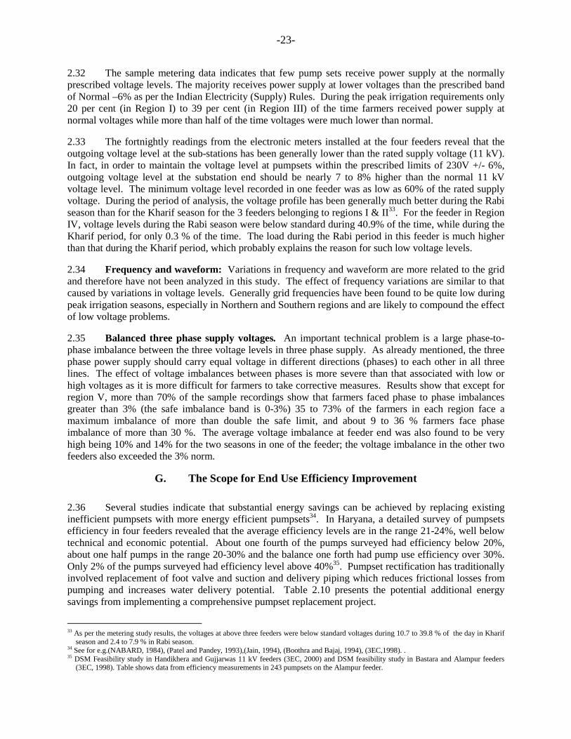
-23-

2.32 The sample metering data indicates that few pump sets receive power supply at the normally prescribed voltage levels. The majority receives power supply at lower voltages than the prescribed band of Normal –6% as per the Indian Electricity (Supply) Rules. During the peak irrigation requirements only 20 per cent (in Region I) to 39 per cent (in Region III) of the time farmers received power supply at normal voltages while more than half of the time voltages were much lower than normal. 2.33 The fortnightly readings from the electronic meters installed at the four feeders reveal that the outgoing voltage level at the sub-stations has been generally lower than the rated supply voltage (11 kV). In fact, in order to maintain the voltage level at pumpsets within the prescribed limits of 230V +/- 6%, outgoing voltage level at the substation end should be nearly 7 to 8% higher than the normal 11 kV voltage level. The minimum voltage level recorded in one feeder was as low as 60% of the rated supply voltage. During the period of analysis, the voltage profile has been generally much better during the Rabi season than for the Kharif season for the 3 feeders belonging to regions I & II33. For the feeder in Region IV, voltage levels during the Rabi season were below standard during 40.9% of the time, while during the Kharif period, for only 0.3 % of the time. The load during the Rabi period in this feeder is much higher than that during the Kharif period, which probably explains the reason for such low voltage levels. 2.34 Frequency and waveform: Variations in frequency and waveform are more related to the grid and therefore have not been analyzed in this study. The effect of frequency variations are similar to that caused by variations in voltage levels. Generally grid frequencies have been found to be quite low during peak irrigation seasons, especially in Northern and Southern regions and are likely to compound the effect of low voltage problems. 2.35 Balanced three phase supply voltages. An important technical problem is a large phase-to-phase imbalance between the three voltage levels in three phase supply. As already mentioned, the three phase power supply should carry equal voltage in different directions (phases) to each other in all three lines. The effect of voltage imbalances between phases is more severe than that associated with low or high voltages as it is more difficult for farmers to take corrective measures. Results show that except for region V, more than 70% of the sample recordings show that farmers faced phase to phase imbalances greater than 3% (the safe imbalance band is 0-3%) 35 to 73% of the farmers in each region face a maximum imbalance of more than double the safe limit, and about 9 to 36 % farmers face phase imbalance of more than 30 %. The average voltage imbalance at feeder end was also found to be very high being 10% and 14% for the two seasons in one of the feeder; the voltage imbalance in the other two feeders also exceeded the 3% norm.

G. The Scope for End Use Efficiency Improvement

2.36 Several studies indicate that substantial energy savings can be achieved by replacing existing inefficient pumpsets with more energy efficient pumpsets34. In Haryana, a detailed survey of pumpsets efficiency in four feeders revealed that the average efficiency levels are in the range 21-24%, well below technical and economic potential. About one fourth of the pumps surveyed had efficiency below 20%, about one half pumps in the range 20-30% and the balance one forth had pump use efficiency over 30%. Only 2% of the pumps surveyed had efficiency level above 40%35. Pumpset rectification has traditionally involved replacement of foot valve and suction and delivery piping which reduces frictional losses from pumping and increases water delivery potential. Table 2.10 presents the potential additional energy savings from implementing a comprehensive pumpset replacement project.

33 As per the metering study results, the voltages at above three feeders were below standard voltages during 10.7 to 39.8 % of the day in Kharif

season and 2.4 to 7.9 % in Rabi season. 34 See for e.g.(NABARD, 1984), (Patel and Pandey, 1993),(Jain, 1994), (Boothra and Bajaj, 1994), (3EC,1998). . 35 DSM Feasibility study in Handikhera and Gujjarwas 11 kV feeders (3EC, 2000) and DSM feasibility study in Bastara and Alampur feeders

(3EC, 1998). Table shows data from efficiency measurements in 243 pumpsets on the Alampur feeder.

-24-

Table 2.10 - Energy savings from implementing comprehensive pumpset replacement program

Step Measure Energy Conservation

Potential

1 Replacement of GI suction pipe and GI foot valve with low friction RPVC pipes and valve.

20%-25%

2 Replacement of suction pipe, foot valve, and delivery pipes. 30%-35%

3 Replacement of suction and delivery pipes, foot valve, and pump with properly sized energy efficient mono-block pump.

40%-45%

2.37 An Integrated Approach to Efficiency. The improvements in power supply quality will encourage the farmers not to install oversized (higher rated) motors, which are generally acquired, to protect against voltage fluctuations. Field studies in Haryana on four 11kV feeders (Bastara, Alampur, Handikera, Gujjarwas) indicate that replacement of pumpsets should be implemented in conjunction with the rehabilitation of the distribution system to maximize energy savings. The rehabilitation of the agricultural feeders will improve power quality supplied to the pumpsets36 to enable them to operate more efficiently, reduce the occurrence of burnouts and thus extend their operational life. A summary of the beneficial characteristics by various stakeholders is presented in Table 2.11 below.

Table 2.11 - Summary of Types of Benefits in Integrated Agricultural DSM Program

Benefit Types of Benefit Term Beneficiary Comments

No Motor Rewinding Rewinding costs eliminated Rs. 1,000-4,000 Annually Farmer Replaced by regular

maintenance

Delayed Pumpset Replacement

Delayed pumpset replacement costs Annually Farmer

Fraction of pumpsets normally replaced each

year

Lower Electricity Costs

Lower power use by metered pumpsets 20%-40%

Annually Farmer

Sales to higher tariff customers or reduced power purchases

Savings in pumpset consumption Annually Utility Depends on WTP, tariffs

and avoided costs

Reduced system losses and transformer failure rate

Lower losses in LT system37 and reduced transformer

failures38 Annually Utility/

farmers

H. Metering Agricultural Consumers

2.38 Metering electricity consumption by farmers will eliminate serious errors in consumption estimates and help conserve electricity and scarce groundwater resources. As earlier indicated, electricity supply to almost 90 per cent agricultural consumers (approx. 283,000) in Haryana is un-metered. The major draw back of not metering all the consumers is that over-estimation by the utilities of electricity sales to agriculture consumers and corresponding underreporting of the T&D losses. Secondly, under the flat rate tariff structure based on connected load of the pumps the marginal cost of electricity use by the consumers is close to zero. This does not provide much incentive to farmers to use electricity for ground water pumping more efficiently, and in fact often leads to wasteful use of not only electricity but precious groundwater. The benefits of DSM as well as its feasibility would be appreciated by the farmers only when the use of electricity is metered and the savings are measurable. Thirdly, flat rate based tariff

36 High efficiency motors are more likely to have higher outages when the quality of power supply is poor. 37 The upgrading to Less LT system lowered LT distribution system losses from 11.7% to 0.85%, in the four representative Haryana feeders

analyzed by USAID. 38 Distribution transformer failure would reduce due to reduction in simultaneous demand of pumpsets with reduced pump capacities.

-25-

structure tends to be more favorable to large farmers compared to small and marginal farmers, as is explained in greater depth in Chapter Three on Costs and Returns. Tariffs based on metering of consumption, can be used more effectively for better targeting of possible subsidies to small and marginal farmers, for instance through implementation of life line rates. Finally, the implementation of capacity based un-metered tariffs is seen to result in a significant loss of revenue for the utilities due to under-reporting of the actual capacity of pumps by the farmers. This tends to encourage discretion for the utility staff to monitor and verify the capacity of pumpsets in the field at regular intervals and may result in increased collusion between consumers and utility staff and corruption. 2.39 Under the farmers attitude survey conducted in Haryana under the study, about 69% of the farmers surveyed favored metered supply. The response is above 73% in regions II, III & IV, whereas in the regions I (46%) and V (29%) lesser proportion of farmers have shown preference for metering. While, no further reasons for the relatively low response in regions V & I have been investigated, both these regions have much higher installed average pump capacity; also in region V where the average groundwater depth is lower 100 feet, several farmers are benefit from the present flat rate tariff structure which provides subsidized tariffs based on depth of ground water. In the farmer’s opinion the main advantages of metering cited include payments related to consumption, reduce wastage of electricity and improvement in power distribution. The major hurdles cited were, meters will be faulty; farmers will directly connect to main line bypassing meter; payment amount would increase; billing will be irregular and readings will be faulty. 2.40 According to HVPN, however, these statements by farmers are not confirmed by the reality on the ground, that is farmers still prefer un-metered connections. For example, metered connections for tubewells has decreased from 107,075 in FY1996 to 73,948 in FY2001, compared to the un-metered connections, which have increased over the same period from 267,274 to 285,128. This, according to HVPN, demonstrates the preference by farmers to opt for un-metered connections rather than metered. Despite the initiation of a program to complete meter installation to all tubewells in two years, HVPN is encountering difficulties in its implementation and various remedial actions have been devised (see Box 2.3).

Box 2.3 – Problems encountered by HVPN in the meter installation and remedial steps

According to HVPN, there are several difficulties encountered in the installation of meters. First, it is necessary to house the meter in a safe weatherproof place, and farmers are not ready to construct the room or shed for the meters. Second, farmers apprehend that once the meter is installed they would be questioned for the extra-consumption for other purposes for the pumping load and their unauthorized load would be detected. Third, farmers do not own the responsibility of safe custody of the meters, as these are not covered under their Power Supply Contract for un-metered connections. Fourth, the utility is unable to recover he cost of the meter nor charge any meter rental or maintenance charges. Fifth, the cost for reading the meters would be an extra financial burden to the utility. Finally, in general most of the farmers oppose installation of meters. HVPN also proposes solutions to the above problems. For example, the un-metered tariff should be totally withdrawn and metering become compulsory that the metering program could become successful. In the meantime, HVPN has already started releasing new connections only on metered basis. In addition, HVPN has proposed the following: The limited purpose of installing the meters is to have an accurate energy audit for the power system. Accordingly, even after installation there will be any impact on consumers’ billing and farmers with un-metered connections will continue to enjoy the existing un-metered tariff. On certain locations where farmers have opposed installation of meters, extensive communication engagement by HVPN staff has resulted in successful installation. • The involvement of village Sarpanch and Member of the Legislative Assembly to persuade reluctant farmers to accept the meter installation

has given positive results.

• The meters are being provided in steel meter cupboards so as to take care of the weather conditions. • No meter security, rentals or upkeep charges are being levied on farmers so that they do not opposed the installation of these meters and the

entire expense is borne by the utility.

-26-

CHAPTER 3

HOW IRRIGATION TECHNOLOGY CHOICES AFFECT FARM INCOMES

A. Introduction 3.1 This chapter compares the gross and net returns to different sources of irrigation. A breakup of the different production costs (particularly, irrigation costs) is also presented to get an idea of much burden the current electricity tariff structure places on farmers and how it compares to the costs of other sources of irrigation available to them. Gross and net farm incomes are observed to vary significantly according to the irrigation technologies used by farmers. In general, electric pump owners in the sample had both the highest gross and the highest net annual farm incomes. Electric pumps owners have gross incomes five times that of farmers who rely on water purchases alone or are solely rain fed. Input costs for pump owners are also significantly higher, as one would expect. Analysis of the production cost components of pump owners indicates the relative importance of tariffs, rewinding expenses and pump maintenance costs and shows how the quality of the electricity supply adversely affects farmers’ bottom lines. Despite higher production costs, the net farm incomes for farmers who own pumps, and in particular electric pumps, are still higher than those of farmers who do not. . Under the current flat rate tariff structure for electricity, tariffs account for a small share of gross income of electric pump owners, but this share is highly regressive across farm sizes. For small and marginal farmers, tariffs account for 2.5 to 13 percent of gross farm income while for medium to large farmers these account for 1 to 6 percent of gross farm income.

B. Gross Farm Income

3.2 Access to irrigation is likely to increase gross returns to land due to several reasons. First, it is likely to lead to more intensive use of land through multiple cropping and cultivation of more water intensive and high valued crops. Second, it helps to reduce some of the risks associated with variation in rainfall. These benefits associated with irrigation are clearly demonstrated in table 3.1 which compares the gross farm income across technology groups and farm size categories. Gross farm income is defined as the sum of the price times the volume of all crops produced during the survey year, irrespective of whether these are self-consumed or sold in the market39. Electric pump owners have the highest average annual gross incomes (Rs.124,090), followed by diesel pump owners (Rs.90,780). Water purchasers and rain fed farmers have gross incomes (Rs. 25,800 and Rs. 27,300 respectively) that are about 20 per cent that of electric pump owners. Canal users’ gross incomes (Rs.76,250) are about 60 per cent) of that of electric pump owners. Among electric pump owners, those who have access to supplemental water, through diesel pumps or canal, have gross incomes about 58 per cent higher than those who are purely dependent on electric pumps. For diesel pump owners who have access to canal water, gross incomes are about 144 per cent higher than those who rely solely on diesel pumps.

39 The gross farm income does not include proceeds from the sale of crop by-products, non-crop activities (e.g. livestock) and sale of water. Total crop production was taken into account here irrespective of whether it was used for self-consumption, as seed for next year or as marketable surplus. Crop production was valued at the price as reported by farmer for the marketed portion.

-27-

Table 3.1: Average Annual Gross Income by Farm Size (Rs.)

Electric pump owners Non-electric diesel pump owners

Canal users

Water purchasers Rainfed Total

Farm size owned

Electric only

Electric and canal

Electric and diesel Total Diesel

only Diesel

and canal Total

Marginal 36,460 41,920 94,010 46,800 28,000 51,240 30,420 21,000 13,810 15,420 25,880 Small 40,520 72,800 65,080 45,980 41,970 66,360 46,840 70,020 30,850 36,680 49,340 Medium 110,480 90,540 111,070 109,520 93,000 147,540 110,480 122,270 69,060 67,770 108,290 Large 240,490 251,250 286,380 259,960 151,970 250,760 211,250 174,820 129,270 110,000 241,360 Overall 102,000 160,550 161,910 124,090 64,460 157,400 90,780 76,250 25,800 27,290 90,940 Gross income is defined as the sum of the price times the production volume of all crops produced. Source: Haryana farmers’ recall survey

3.3 The average gross income of marginal farmers who own electric pumps is almost three times that of their counterparts in the rainfed and water purchasers category. In particular, the gross income of marginal farmers owning both electric and diesel pumps is very high, almost 6 times that of the rainfed marginal farmers. One of the reasons for this is that ownership of pumps allows marginal farmers with very small landholdings to lease in more land and thus increase their scale of operation (see Chapter I). This is an important advantage associated with ownership of productive assets like wells and pumps for land-poor farmers.

3.4 Gross incomes are a function of not only the irrigation technology source but also the scale of cultivation, amongst other factors.40 Therefore, as expected, gross incomes increase with farm size within each technology group in table 3.1. To enable a better understanding of the gross returns to a unit of cultivated land across irrigation technologies, the above values are normalized to a per hectare basis in table 3.2. It is interesting to observe that on a per hectare basis, gross returns vary much less across technology groups. It is also noteworthy that gross returns per hectare are higher for pure canal users and diesel pump owners relative to electric pump owners. Within the category of electric pump owners, gross returns per hectare are highest for farmers who have both an electric pump and a diesel pump. In subsequent sections, it is discussed how diesel pumps increase the productivity of electric pump owners by helping to cope with poor conditions of electricity supply.

Table 3.2 Gross Farm Income per hectare of Net Cultivated Area (Rs./Ha.)

Electric pump owners Non-electric diesel pump owners Canal users

Water purchasers Rainfed Total Region/

farm size category Electric

only Electric and canal

Electric and diesel Total Diesel

only Diesel

and canal Total

Marginal 29,750 27,960 42,220 31,940 34,250 35,430 34,370 30,580 26,020 27,480 29,500 Small 24,950 27,400 25,650 25,170 27,130 41,260 29,960 51,950 22,870 27,270 31,980 Medium 33,120 26,210 30,470 31,710 30,830 37,650 33,020 41,140 29,690 28,340 33,120 Large 27,100 24,360 30,030 27,940 28,250 35,960 32,870 33,770 18,770 27,230 29,010 Overall 29,200 25,600 31,040 29,530 30,330 37,660 32,400 40,160 25,650 27,570 31,070 Source: Haryana farmers’ recall survey

C. Production Costs 3.5 This section examines the structure of production costs across different irrigation technology groups. Total farm production costs were aggregated into 4 major categories: hired labor, own labor, materials and irrigation costs. These costs are presented as a percentage of gross income to facilitate comparisons across different types of technologies in Table 3.3.

40 The separate impacts of these factors are tested more rigorously in Chapter 5.

-28-

3.6 Irrigation costs for pump users dwarf those for canal users and water purchasers.. The results also suggest that on average, all types of electric and diesel pump owners tend to use various materials (fertilizers, pesticides, farm cultivation services such as tractors and animal draft, non-irrigation diesel, etc) more intensively than non-pump owners (canal, water purchasers and rainfed). On average, these costs account for about 20-22 per cent of gross income for pump owners, compared to about 15-16 per cent of non-pump owners. There is greater variation in the share of labor (hired and own) in gross income among different technologies. Not only do canal users use materials less intensively, they also appear to use labor less intensively as well, having the lowest share of labor costs (5 per cent).

3.7 Among both electric and diesel pump owners, the share of irrigation cost in gross income is regressive, that is, it tends to increase as farm size decreases. But for electric pump owners this is more pronounced because of the regressive nature of the present flat rate tariff structure. The degree of disparity in share of irrigation costs between marginal and large farmers varies considerably by technology. Marginal farmers who only use electric pumps pay more than a third of their gross income for irrigation. This implies that small and marginal farmers, especially those purely dependent on electric or diesel pumps, would tend to be more vulnerable to increases in irrigation costs. The survey also shows that the cost share of irrigation is highest for the pure electric pump owners and the pure diesel pump owners (around 24 to 31 per cent)41. Access to complementary sources of water, especially canal, reduces irrigation cost share by 8 to 15 percentage points. The structure of production costs also varies across regions. Annexes 5, Tables A2.25-27 provide the regional results.

41 The decomposition of irrigation costs into fixed and variable costs is explained in greater detail in the next subsection.

-29-

Table 3.3 - Production Cost as Percent of Gross Income

Irrigation Cost Region/

farm size category

Hired Labor Own Labor* Materials Variable Costs

Annualized Fixed Cost

of Pump and Well

Total Total Cost

1. Electric pump users only Marginal 8.81 13.08 21.97 25.74 12.1 38.4 82.4 Small 7.20 10.43 22.53 16.07 11.9 28.7 68.7 Medium 6.33 5.90 21.06 9.08 8.6 18.3 51.7 Large 8.03 5.39 23.97 8.17 6 14.9 53.7 Overall 7.43 8.52 22.19 14.54 9.7 24.9 63.5 2.Electric and Canal users Marginal 10.72 7.06 19.44 8.38 3.6 12.2 49.2 Small 6.21 9.44 19.68 5.46 8.3 13.8 49.1 Medium 6.7 4.65 19.47 9.71 7.6 17.3 48.1 Large 7.13 5.26 21.55 5.53 3.1 8.8 40 Overall 7.02 5.71 20.46 7.15 5.4 12.7 44.6 3. Electric &Diesel pump users Marginal 6.29 6.55 20.1 11.06 3.9 15.7 48.4 Small 7.81 7 19.56 12.24 10.3 23.6 58.4 Medium 5.73 5.17 19.42 9.26 8.6 18 48.3 Large 6.75 4.32 19.81 6.2 5.8 12.4 43.5 Overall 6.33 5.22 19.63 8.71 7.4 16.5 47.8 4. Diesel pump users only Marginal 7.70 6.83 21.82 14.96 30.3 45.2 81.6 Small 10.10 6.68 20.34 12.22 19.1 31.3 68.4 Medium 12.69 8.16 24.46 10.99 13.2 24.2 69.5 Large 13.53 7.00 21.36 8.34 8.1 16.5 58.3 Overall 10.60 7.23 22.17 12.21 19.2 31.4 71.4 5. Diesel and Canal users Marginal 6.19 7.82 21.41 13.51 17.9 31.4 66.8 Small 9.09 5.99 20.24 12.24 14.2 26.5 61.8 Medium 11.50 7.41 22.03 9.22 8.4 17.6 58.6 Large 14.50 8.00 22.59 10.38 4.1 14.4 59.5 Overall 11.58 7.35 21.80 10.55 8.9 19.5 60.2 6. Canal users only Marginal 4.58 5.43 17.08 0.47 0.47 27.56 Small 5.47 4.94 14.29 0.42 0.42 25.13 Medium 6.27 5.98 15.63 0.51 0.51 28.39 Large 5.75 5.33 17.82 0.48 0.48 29.39 Overall 5.40 5.42 15.91 0.46 0.46 27.20 7. Water Purchasers Marginal 5.87 11.48 14.90 10.44 10.44 42.69 Small 10.00 11.12 20.26 8.76 8.76 50.15 Medium 8.54 8.35 14.36 4.16 4.16 35.41 Large 6.68 7.42 36.59 12.42 12.42 63.11 Overall 6.97 10.97 16.37 9.48 9.48 43.79 8. Rainfed Marginal 7.67 11.40 15.01 34.07 Small 10.26 6.09 15.75 32.10 Medium 7.63 5.86 16.31 29.80 Large 13.08 5.42 17.99 36.49 Overall 8.13 9.72 15.34 33.20 Notes: * Imputed at village level wages for male and female labor. Material costs include fertilizers, pesticides, etc. See Annex Tables A2.25-37 for disaggregated values by region.

-30-

D. Decomposition of Irrigation Costs 3.8 Total irrigation costs can be decomposed into two broad categories, fixed and variable costs. The fixed cost component of irrigation refers to the annualized amortized value of the initial investment in well, pumps and related equipment such as sheds, collection tank if any etc. For the non pump owning sample categories this component is almost zero. Variable costs include yearly expenses on electricity tariffs, motor rewinding after a burnout , pump maintenance, diesel used for pumping, water purchases and canal fees. For canal users, variable costs include canal fees. In Haryana, canal fees vary across crop and season and range from Rs.18/acre for wheat42 to Rs.45/acre for rice. Figures 3.1 and 3.2 illustrate the break down in irrigation costs as a percentage of gross farm income across farm sizes for electric pump owners. 3.9 Electricity tariff rates in Haryana. Farmers in Haryana have the choice of being charged for their consumption either on the basis of per unit of consumption (metered rate) or on the basis of a flat rate per installed HP per month43. In FY2000, there were 69,155 metered connections representing about 20 per cent of all connections.. Unmetered connections, which have been increasing over the past four years, were 283,720. At present there are no charges for getting a connection or for registration. However, if the connection is disconnected there is a re-connection charge of Rs 250 per connection. Farmers opting for metered tariff have to pay Rs 1,000 for security deposit, meter service charge of Rs 20 per month and minimum charge of Rs 540/BHP/year. Typically, in areas where a single crop is grown in the year, farmers prefer to opt for metered tariff. But there is no data available as to how many meters are actually working in the field. Among the sample of farmers in the survey, 94 per cent were not metered but rather billed on flat rates based on water table depth (see table 3.4).

Table 3.4. Electricity tariffs for agricultural sector in Haryana in FY2000

Depth of borewell in feet Metered charges (Rates/kWh) Fixed rates per BHP/month Upto 100 Rs 0.50 Rs 65

101 to 150 Rs 0.38 Rs 50 151 to 200 Rs 0.31 Rs 40 Above 200 Rs 0.23 Rs 30

3.10 In the survey, sample farmers were asked about the actual tariff they paid in each season. However, the data on this aspect has not been collected very well. 44 The procedure for imputing the cost of tariff is explained in the report on methodology. But for a variety of reasons, such as illegal connections or a discrepancy between the HP records of the utility and actual pump size, and non-full payment of bills etc., farmers often pay less than the tariff cost imputation. While it is difficult to explain the exact magnitude of the discrepancy between the actual amount paid by farmers and the tariff cost imputation, it is clear that the latter defines the upper bound on the actual cost borne by farmers. The results on tariff costs in this section need to be interpreted keeping this in mind. 3.11 Tariff share in gross income: For the average electric pump owner in the sample, electricity tariffs account at the low end for about 1 per cent (for those who use electric with diesel pumps) to 9 per

42 For wheat, in Kharif channels the cost is Rs. 18/acre. In non-Khraif channels the cost is Rs. 37/acre. 43 Interestingly, in the Attitude survey farmers reported that although theoretically they have a choice between metered and un-metered connections, the HVPNL field staff does not encourage metered power supply for agricultural consumers (ORG Attitude Survey Report, p.40). 44 This is because the period over which the bill is paid differs across farmers. It ranges from payment once every month in region I to payment once every 4 months in region 5 (ORG, Attitude Survey Report). Unfortunately the period over which the bill was paid by each farmer was not recorded satisfactorily in the recall survey. Also it was observed that farmers often do not pay the full amount due in any bill. Thus the amount reported by the farmer in any season may not be a true indicator of the total amount due to him.

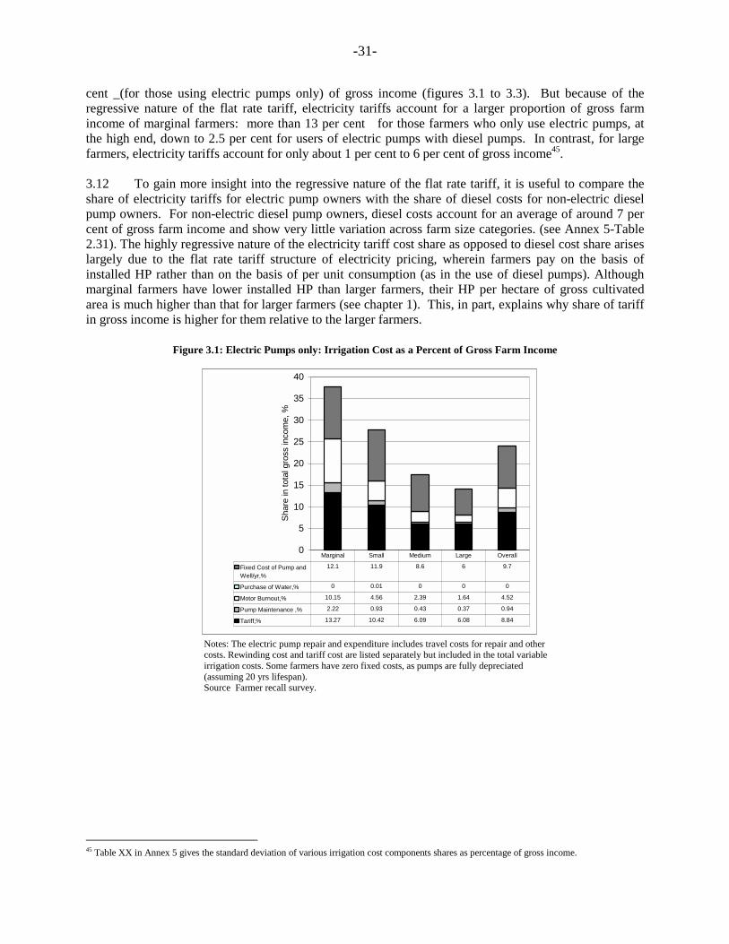
-31-

cent _(for those using electric pumps only) of gross income (figures 3.1 to 3.3). But because of the regressive nature of the flat rate tariff, electricity tariffs account for a larger proportion of gross farm income of marginal farmers: more than 13 per cent for those farmers who only use electric pumps, at the high end, down to 2.5 per cent for users of electric pumps with diesel pumps. In contrast, for large farmers, electricity tariffs account for only about 1 per cent to 6 per cent of gross income45. 3.12 To gain more insight into the regressive nature of the flat rate tariff, it is useful to compare the share of electricity tariffs for electric pump owners with the share of diesel costs for non-electric diesel pump owners. For non-electric diesel pump owners, diesel costs account for an average of around 7 per cent of gross farm income and show very little variation across farm size categories. (see Annex 5-Table 2.31). The highly regressive nature of the electricity tariff cost share as opposed to diesel cost share arises largely due to the flat rate tariff structure of electricity pricing, wherein farmers pay on the basis of installed HP rather than on the basis of per unit consumption (as in the use of diesel pumps). Although marginal farmers have lower installed HP than larger farmers, their HP per hectare of gross cultivated area is much higher than that for larger farmers (see chapter 1). This, in part, explains why share of tariff in gross income is higher for them relative to the larger farmers.

Figure 3.1: Electric Pumps only: Irrigation Cost as a Percent of Gross Farm Income

Notes: The electric pump repair and expenditure includes travel costs for repair and other costs. Rewinding cost and tariff cost are listed separately but included in the total variable irrigation costs. Some farmers have zero fixed costs, as pumps are fully depreciated (assuming 20 yrs lifespan). Source Farmer recall survey.

45 Table XX in Annex 5 gives the standard deviation of various irrigation cost components shares as percentage of gross income.

0

5

10

15

20

25

30

35

40

Shar

e in

tota

l gro

ss in

com

e, %

Fixed Cost of Pump andWell/yr,%

12.1 11.9 8.6 6 9.7

Purchase of Water,% 0 0.01 0 0 0

Motor Burnout,% 10.15 4.56 2.39 1.64 4.52

Pump Maintenance ,% 2.22 0.93 0.43 0.37 0.94

Tariff,% 13.27 10.42 6.09 6.08 8.84

Marginal Small Medium Large Overall

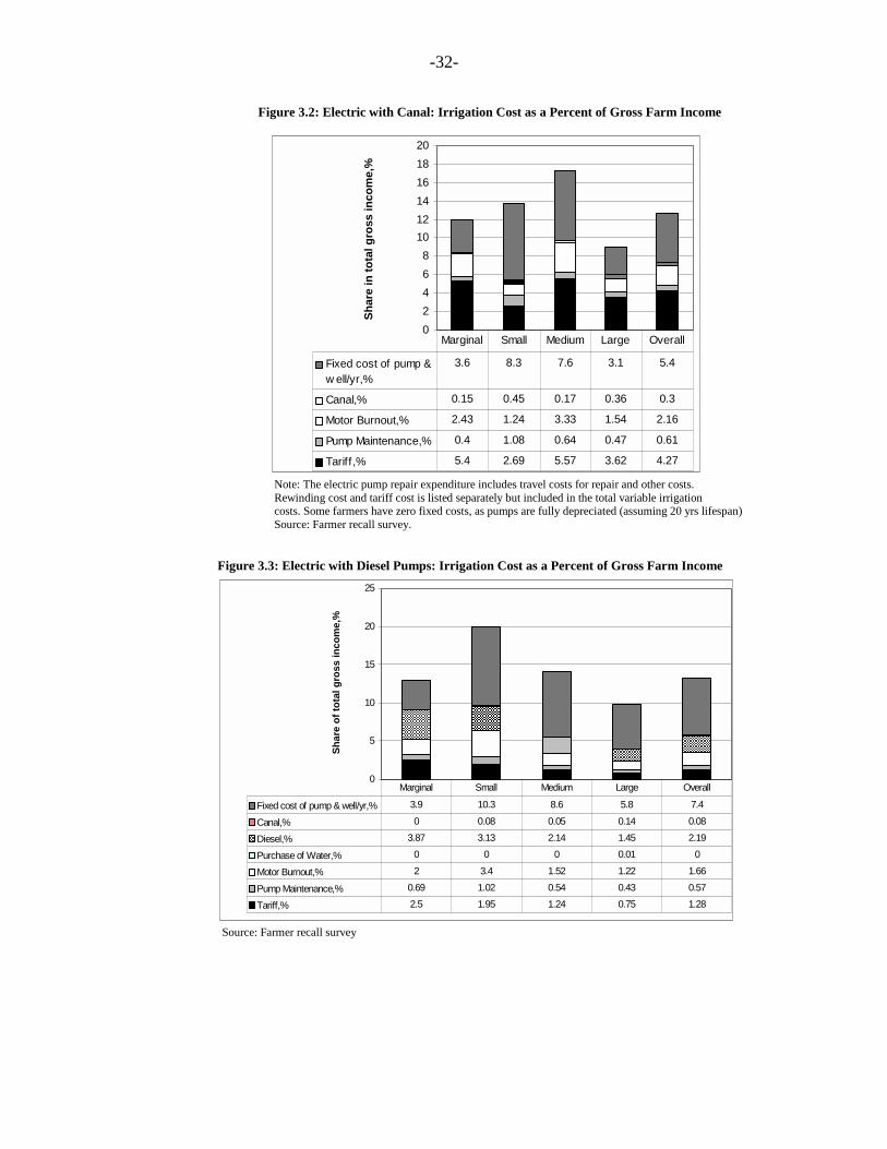
-32-

Figure 3.2: Electric with Canal: Irrigation Cost as a Percent of Gross Farm Income

Note: The electric pump repair expenditure includes travel costs for repair and other costs. Rewinding cost and tariff cost is listed separately but included in the total variable irrigation costs. Some farmers have zero fixed costs, as pumps are fully depreciated (assuming 20 yrs lifespan) Source: Farmer recall survey.

Figure 3.3: Electric with Diesel Pumps: Irrigation Cost as a Percent of Gross Farm Income

Source: Farmer recall survey

02468

101214161820

Shar

e in

tota

l gro

ss in

com

e,%

Fixed cost of pump &w ell/yr,%

3.6 8.3 7.6 3.1 5.4

Canal,% 0.15 0.45 0.17 0.36 0.3

Motor Burnout,% 2.43 1.24 3.33 1.54 2.16

Pump Maintenance,% 0.4 1.08 0.64 0.47 0.61

Tariff ,% 5.4 2.69 5.57 3.62 4.27

Marginal Small Medium Large Overall

0

5

10

15

20

25

Shar

e of

tota

l gro

ss in

com

e,%

Fixed cost of pump & well/yr,% 3.9 10.3 8.6 5.8 7.4

Canal,% 0 0.08 0.05 0.14 0.08

Diesel,% 3.87 3.13 2.14 1.45 2.19

Purchase of Water,% 0 0 0 0.01 0

Motor Burnout,% 2 3.4 1.52 1.22 1.66

Pump Maintenance,% 0.69 1.02 0.54 0.43 0.57

Tariff,% 2.5 1.95 1.24 0.75 1.28

Marginal Small Medium Large Overall

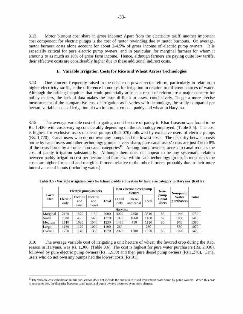
-33-

3.13 Motor burnout cost share in gross income: Apart from the electricity tariff, another important cost component for electric pumps is the cost of motor rewinding due to motor burnouts. On average, motor burnout costs alone account for about 2-4.5% of gross income of electric pump owners. It is especially critical for pure electric pump owners, and in particular, for marginal farmers for whom it amounts to as much as 10% of gross farm income. Hence, although farmers are paying quite low tariffs, their effective costs are considerably higher due to these additional indirect costs.

E. Variable Irrigation Costs for Rice and Wheat Across Technologies 3.14 One concern frequently raised in the debate on power sector reform, particularly in relation to higher electricity tariffs, is the difference in outlays for irrigation in relation to different sources of water. Although the pricing inequities that could potentially arise as a result of reform are a major concern for policy makers, the lack of data makes the issue difficult to assess conclusively. To get a more precise measurement of the comparative cost of irrigation as it varies with technology, the study compared per hectare variable costs of irrigation of two important crops – paddy and wheat in Haryana.

3.15 The average variable cost of irrigating a unit hectare of paddy in Kharif season was found to be Rs. 1,420, with costs varying considerably depending on the technology employed. (Table 3.5). The cost is highest for exclusive users of diesel pumps (Rs.2,070) followed by exclusive users of electric pumps (Rs. 1,720). Canal users who do not own any pumps had the lowest costs. The disparity between costs borne by canal users and other technology groups is very sharp; pure canal users’ costs are just 4% to 8% of the costs borne by all other non-canal categories46. Among pump owners, access to canal reduces the cost of paddy irrigation substantially. Although there does not appear to be any systematic relation between paddy irrigation cost per hectare and farm size within each technology group, in most cases the costs are higher for small and marginal farmers relative to the other farmers, probably due to their more intensive use of inputs (including water.)

Table 3.5 - Variable irrigation costs for Kharif paddy cultivation by farm size category in Haryana (Rs/Ha)

Electric pump owners Non-electric diesel pump owners

Farm Size Electric

only

Electric and

canal

Electric and

diesel Total Diesel

only Diesel

and canal Total

Non-pump Canal Users

Non-pump Water

purchasersTotal

Haryana Marginal 2160 1470 1150 2000 4000 2250 3810 86 1040 1730 Small 1940 450 1420 1770 1090 1660 1180 87 1090 1410 Medium 1510 1620 1540 1530 1460 410 1150 80 970 1360 Large 1180 1120 1000 1100 260 260 580 1070 Overall 1720 1140 1330 1570 2070 1200 1920 85 1020 1420

3.16 The average variable cost of irrigating a unit hectare of wheat, the favored crop during the Rabi season in Haryana, was Rs. 1,300. (Table 3.6) The cost is highest for pure water purchasers (Rs. 2,030), followed by pure electric pump owners (Rs. 1,930) and then pure diesel pump owners (Rs.1,270). Canal users who do not own any pumps had the lowest costs (Rs.91).

46 The variable cost calculation in this sub-section does not include the annualized fixed investment costs borne by pump owners. When this cost is accounted for, the disparity between canal users and pump owners becomes even more sharper.

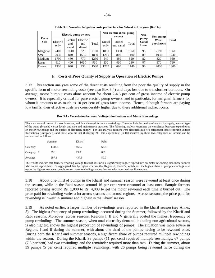
-34-

Table 3.6: Variable Irrigation costs per hectare for Wheat in Haryana (Rs/Ha)

Electric pump owners Non-electric diesel pump owners Farm

Size Electric only

Electric and

canal

Electric and

diesel Total Diesel

only Diesel

and canal Total

Non-pump Canal Users

Non-pump Water

purchasersTotal

Marginal 2400 1040 820 2100 1890 1350 1850 95 2190 1660 Small 2030 840 1630 1890 1210 800 1100 89 1930 1240 Medium 1790 480 770 1230 540 480 520 82 820 950 Large 910 400 1030 930 230 430 280 87 570 760 Overall 1930 640 930 1530 1270 690 1140 90 2030 1300

F. Costs of Poor Quality of Supply in Operation of Electric Pumps

3.17 This section analyzes some of the direct costs resulting from the poor the quality of supply in the specific form of motor rewinding costs (see also Box 3.4) and days lost due to transformer burnouts. On average, motor burnout costs alone account for about 2-4.5 per cent of gross income of electric pump owners. It is especially critical for pure electric pump owners, and in particular, for marginal farmers for whom it amounts to as much as 10 per cent of gross farm income. Hence, although farmers are paying low tariffs, their effective costs are considerably higher due to these additional indirect costs.

Box 3.4 - Correlation between Voltage Fluctuations and Motor Rewindings There are several causes of motor burnouts, and thus the need for motor rewindings. These include the quality of electricity supply, age and type of the pump (branded versus local), and care and maintenance practices. The following analysis examines the correlation between expenditures on motor rewindings and the quality of electricity supply. For this analysis, farmers were classified into two categories: those reporting voltage fluctuations (Category 1) and those who did not (Category 2). The expenditure (in Rs) incurred by these two categories of farmers can be summarized as follows:

Summer Kharif Rabi

Category 1344.5 468.7 63.8

Category 2 89.1 29.8 8.2

Average 297.1 437.3 59.9

The results indicate that farmers reporting voltage fluctuations incur a significantly higher expenditure on motor rewinding than those farmers who do not report them. Disaggregated data by region, confirm that Regions I, II and V, which post the highest share of pump rewindings, also report the highest average expenditures on motor rewindings among farmers who report voltage fluctuations.

3.18 About one-third of pumps in the Kharif and summer season were rewound at least once during the season, while in the Rabi season around 16 per cent were rewound at least once. Sample farmers reported paying around Rs. 1,000 to Rs. 4,000 to get the motor rewound each time it burned out. The price paid for rewinding varies a lot across seasons and across regions. Across seasons, the price paid for rewinding is lowest in summer and highest in the Kharif season. 3.19 As noted earlier, a larger number of rewindings were reported in the kharif season (see Annex 5). The highest frequency of pump rewindings occurred during the Summer, followed by the Kharif and Rabi seasons. Moreover, across seasons, Regions I, II and V generally posted the highest frequency of pump rewindings. The summer season, when total electricity demand, including non-agricultural sectors, is also highest, shows the highest proportion of rewindings of pumps. The situation was more severe in Regions I and II during the summer, with about one third of the pumps having to be rewound once. During both the Kharif and summer seasons, a significant share of pumps required multiple rewindings within the season. During the Kharif, 98 pumps (11 per cent) required multiple rewindings; 67 pumps (7.5 per cent) had two rewindings and the remainder required more than two. During the summer, about 39 pumps (5 per cent) required multiple rewindings, with 26 pumps being rewound twice during the

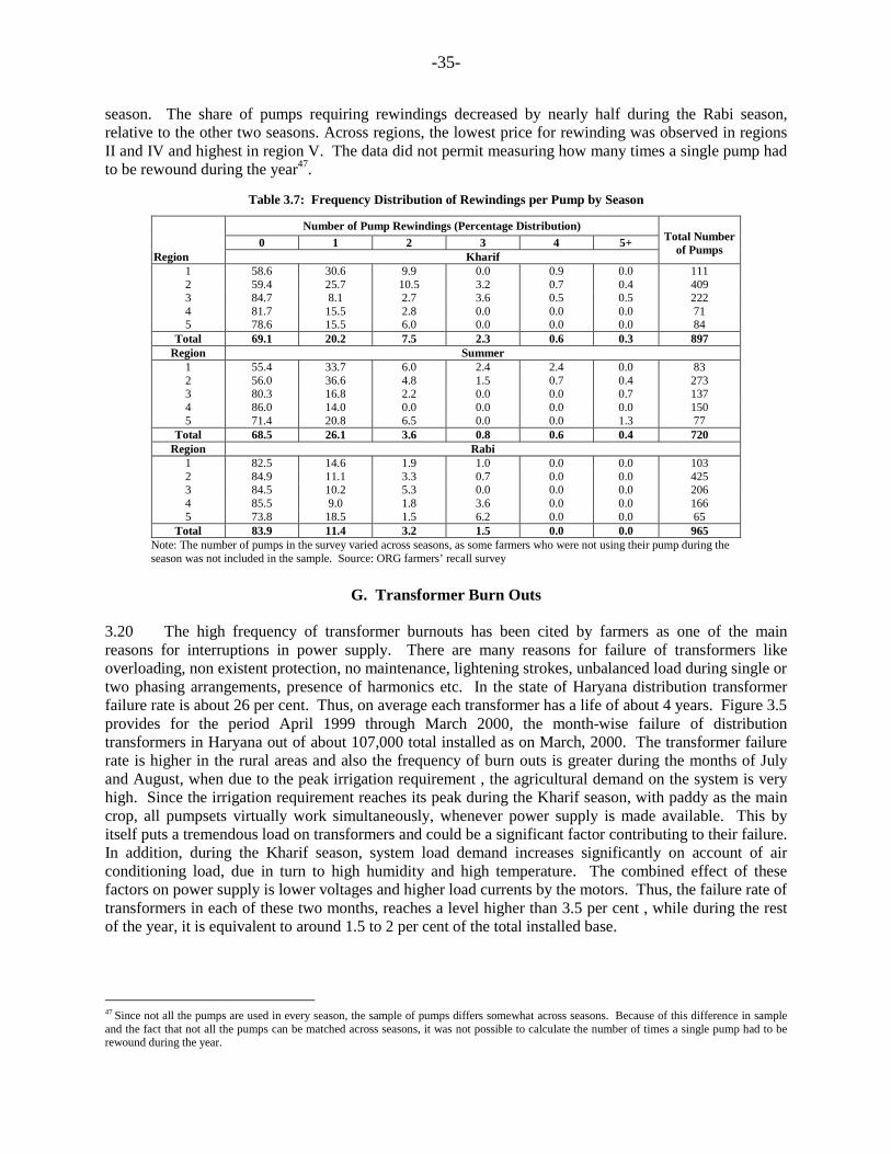
-35-

season. The share of pumps requiring rewindings decreased by nearly half during the Rabi season, relative to the other two seasons. Across regions, the lowest price for rewinding was observed in regions II and IV and highest in region V. The data did not permit measuring how many times a single pump had to be rewound during the year47.

Table 3.7: Frequency Distribution of Rewindings per Pump by Season

Number of Pump Rewindings (Percentage Distribution) 0 1 2 3 4 5+ Region Kharif

Total Number

of Pumps

1 58.6 30.6 9.9 0.0 0.9 0.0 111 2 59.4 25.7 10.5 3.2 0.7 0.4 409 3 84.7 8.1 2.7 3.6 0.5 0.5 222 4 81.7 15.5 2.8 0.0 0.0 0.0 71 5 78.6 15.5 6.0 0.0 0.0 0.0 84

Total 69.1 20.2 7.5 2.3 0.6 0.3 897 Region Summer

1 55.4 33.7 6.0 2.4 2.4 0.0 83 2 56.0 36.6 4.8 1.5 0.7 0.4 273 3 80.3 16.8 2.2 0.0 0.0 0.7 137 4 86.0 14.0 0.0 0.0 0.0 0.0 150 5 71.4 20.8 6.5 0.0 0.0 1.3 77

Total 68.5 26.1 3.6 0.8 0.6 0.4 720 Region Rabi

1 82.5 14.6 1.9 1.0 0.0 0.0 103 2 84.9 11.1 3.3 0.7 0.0 0.0 425 3 84.5 10.2 5.3 0.0 0.0 0.0 206 4 85.5 9.0 1.8 3.6 0.0 0.0 166 5 73.8 18.5 1.5 6.2 0.0 0.0 65

Total 83.9 11.4 3.2 1.5 0.0 0.0 965 Note: The number of pumps in the survey varied across seasons, as some farmers who were not using their pump during the season was not included in the sample. Source: ORG farmers’ recall survey

G. Transformer Burn Outs

3.20 The high frequency of transformer burnouts has been cited by farmers as one of the main reasons for interruptions in power supply. There are many reasons for failure of transformers like overloading, non existent protection, no maintenance, lightening strokes, unbalanced load during single or two phasing arrangements, presence of harmonics etc. In the state of Haryana distribution transformer failure rate is about 26 per cent. Thus, on average each transformer has a life of about 4 years. Figure 3.5 provides for the period April 1999 through March 2000, the month-wise failure of distribution transformers in Haryana out of about 107,000 total installed as on March, 2000. The transformer failure rate is higher in the rural areas and also the frequency of burn outs is greater during the months of July and August, when due to the peak irrigation requirement , the agricultural demand on the system is very high. Since the irrigation requirement reaches its peak during the Kharif season, with paddy as the main crop, all pumpsets virtually work simultaneously, whenever power supply is made available. This by itself puts a tremendous load on transformers and could be a significant factor contributing to their failure. In addition, during the Kharif season, system load demand increases significantly on account of air conditioning load, due in turn to high humidity and high temperature. The combined effect of these factors on power supply is lower voltages and higher load currents by the motors. Thus, the failure rate of transformers in each of these two months, reaches a level higher than 3.5 per cent , while during the rest of the year, it is equivalent to around 1.5 to 2 per cent of the total installed base.

47 Since not all the pumps are used in every season, the sample of pumps differs somewhat across seasons. Because of this difference in sample and the fact that not all the pumps can be matched across seasons, it was not possible to calculate the number of times a single pump had to be rewound during the year.

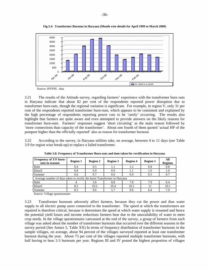
-36-

Fig.3.4: Transformer Burnout in Haryana (Month wise details for April 1999 to March 2000)

0500

100015002000

25003000

3500

4000

Apr-99

Jun-99

Aug-99Oct-

99

Dec-99

Feb-00

No. failed in a month Source: HVPNL data

3.21 The results of the Attitude survey, regarding farmers’ experience with the transformer burn outs in Haryana indicate that about 82 per cent of the respondents reported power disruption due to transformer burn-outs, though the regional variation is significant. For example, in region V, only 31 per cent of the respondents reported transformer burn-outs, which appears to be consistent and explained by the high percentage of respondents reporting power cuts to be ‘rarely’ occurring. The results also highlight that farmers are quite aware and even attempted to provide answers on the likely reasons for transformer burn-outs. Farmers’ responses suggest ‘short circuiting’ as the main reason followed by ‘more connections than capacity of the transformer’. About one fourth of them quoted ‘actual HP of the pumpset higher than the officially reported’ also as reason for transformer burnout. 3.22 According to the survey, in Haryana utilities take, on average, between 4 to 11 days (see Table 3.9 for region wise break-up) to replace a failed transformer.

Table 3.8: Frequency of Transformer Burn-outs and time taken for rectification in Haryana

Frequency of T/F burn-outs in seasons Region 1 Region 2 Region 3 Region 4 Region 5 All

Regions Rabi 0.4 0.5 1.1 1.2 0.8 0.8 Kharif 0.8 0.9 0.9 1.1 1.0 1.0 Summer 0.6 0.7 0.6 0.9 0.5 0.7 Average number of days taken to rectify the burnt Transformer in Haryana

Rabi 4 3.6 8.8 7.8 7.9 6.4 Kharif 8.5 10.5 10.4 10.1 11 10.1 Summer 8.3 9.6 5.7 9.6 6.4 7.9 Source: Village questionnaire

3.23 Transformer burnouts adversely affect farmers, because they cut the power and thus water supply to all electric pump users connected to the transformer. The speed at which the transformers are repaired is therefore critical, because it determines the speed at which water supply is resumed and hence the potential yield losses and income reductions farmers bear due to the unavailability of water to meet crop needs. In the village questionnaire canvassed at the end of the survey, a group of farmers from each village was asked about the number of transformer burnouts that occurred over the different seasons in the survey period (See Annex 5, Table XX) In terms of frequency distribution of transformer burnouts in the sample villages, on average, about 94 percent of the villages surveyed reported at least one transformer burnout during the year. About 73 per cent of the villages reported multiple transformer burnouts, with half having to bear 2-3 burnouts per year. Regions III and IV posted the highest proportion of villages

-37-

reporting multiple transformer burnouts. In Region III and IV respectively, about 32 per cent and 44 per cent of the villages reported 4-6 transformer burnouts per year. By contrast, Regions I, II and V, had relatively “better” performance mostly having to bear 2-3 transformer burnouts per year. 3.24 Across seasons, the largest share of villages reporting transformer burnouts was in Kharif, with 70 per cent of the villages reporting 1-2 burnouts (see Annex 5, Table 3.11). Regions II and IV had the highest share of villages with burnouts. In the summer time when overall electricity demand (including demand from non-agricultural sector) is highest, over 60 per cent of the villages in Regions I, II, IV reported transformer burnouts) By contrast, Regions III, IV and V exhibited the highest number of villages reporting transformer burnouts during the rabi season. 3.25 Average Number of Days Taken to Repair Transformers. On average, it takes about 6 days to repair burnt out transformers during the Rabi Season, 8 days during the Summer Season and 10 days during the Kharif season (Figure 3.6). These averages, however, mask the variability in time taken across different villages. Of the villages reporting a transformer burnout during the year, 41 per cent reported it took 10-12 days for the transformer to be repaired, 34 per cent reported 13-15 days and 25 per cent reported 7-9 days. As transformer burnouts are likely to occur during peak periods of water, and thus electricity demand among users, the long delays in resumption of power supply is likely to have a significant impact on yields. This is explored more rigorously in subsequent sections.

H. Per unit tariff paid by farmers (including cost due to poor quality) 3.26 The tariff paid by farmers per unit of electricity consumption, including and excluding the costs due to poor quality of supply in the form of motor rewinding costs, was analyzed to try to estimate how much poor quality supply increased per unit costs. The results (shown in Annex VI) show that poor quality of supply can increase per unit costs between 23 and 33 per cent.

3.27 The calculations are based only on the sample of pumps that were metered. Since it is not exactly clear as to what proportion of motor rewinding costs can be attributed to poor quality of supply and what can be attributed to factors such as age of motor, regular wear and tear, previous history of rewindings etc., several different assumptions are made regarding the proportion of costs that can be attributed to poor quality. The average per unit nominal tariff for the entire year is Rs. 0.66 per kWh. Under the most conservative scenario, where only 70 per cent of the entire costs of motor rewindings are attributed to poor quality of supply, the effective tariff works out to be Rs. 0.81 per kWh. Under this assumption, poor quality of supply raises the per unit tariff paid by farmers by around 23 per cent. On the other hand, if the entire cost of motor rewinding are attributed to poor quality of supply, effective per unit tariff works out to be Rs. 0.88 per kWh. Under this assumption, poor quality of supply raises the per unit tariff paid by farmers by around 33 per cent. Note that the poor quality of supply has several other important effects on farmers besides resulting in additional expenditures on motor rewindings. Thus, for instance, the loss in crop yields due to lack of water in the time period it takes to get the motor rewound also needs to be taken into account. (The loss in income due to these yield losses is estimated in the econometric model).

3.28 The tariff rate used here is based on average groundwater depth reported at district level. A weighted average of the different districts in each region was taken to estimate the tariff rate at the regional level. The weights here are proportional to the number of metered pumps in each district in the sample. The average cost of motor rewinding per pump is taken from the farmers’ recall data.

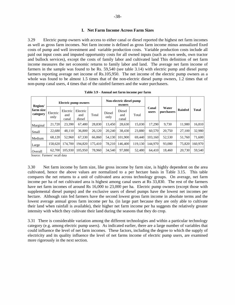
-38-

I. Net Farm Income Across Farm Sizes 3.29 Electric pump owners with access to either canal or diesel reported the highest net farm incomes as well as gross farm incomes. Net farm income is defined as gross farm income minus annualized fixed costs of pump and well investment and variable production costs. Variable production costs include all paid out input costs and imputed opportunity costs for all owned inputs (such as own seeds, own tractor and bullock services), except the costs of family labor and cultivated land This definition of net farm income measures the net economic returns to family labor and land. The average net farm income of farmers in the sample was found to be Rs. 59,540 (see table 3.14) with electric pump and diesel pump farmers reporting average net income of Rs.105,950. The net income of the electric pump owners as a whole was found to be almost 1.5 times that of the non-electric diesel pump owners, 1.2 times that of non-pump canal users, 4 times that of the rainfed farmers and the water purchasers.

Table 3.9 - Annual net farm income per farm

Electric pump owners Non-electric diesel pump owners Region/

farm size category Electric

only

Electric and

canal

Electric and

diesel Total Diesel

only

Diesel and

canal Total

Canal users

Water purchasers Rainfed Total

Marginal 21,720 23,390 67,480 28,830 13,450 28,630 15,030 17,290 9,730 11,980 16,810

Small 22,680 48,110 36,800 26,120 20,240 38,430 23,880 60,570 20,750 27,100 32,980

Medium 68,120 52,960 67,330 66,860 54,130 101,900 69,440 103,160 52,530 51,760 71,600

Large 158,620 174,700 194,820 175,410 78,210 146,400 119,130 144,970 93,080 75,820 160,970

Overall 62,700 105,930 105,950 78,960 34,540 97,880 52,480 64,410 18,460 20,730 59,540Source: Farmers’ recall data

3.30 Net farm income by farm size, like gross income by farm size, is highly dependent on the area cultivated, hence the above values are normalized to a per hectare basis in Table 3.15. This table compares the net returns to a unit of cultivated area across technology groups. On average, net farm income per ha of net cultivated area is highest among canal users at Rs 33,830. The rest of the farmers have net farm incomes of around Rs 16,000 to 23,000 per ha. Electric pump owners (except those with supplemental diesel pumps) and the exclusive users of diesel pumps have the lowest net incomes per hectare. Although rain fed farmers have the second lowest gross farm income in absolute terms and the lowest average annual gross farm income per ha. (in large part because they are only able to cultivate their land when rainfall is available), their higher net farm income per ha suggests the relatively greater intensity with which they cultivate their land during the seasons that they do crop. 3.31 There is considerable variation among the different technologies and within a particular technology category (e.g. among electric pump users). As indicated earlier, there are a large number of variables that could influence the level of net farm incomes. These factors, including the degree to which the supply of electricity and its quality influence the level of net farms income of electric pump users, are examined more rigorously in the next section.

-39-

Table 3.10 - Net Farm Income per Net Cultivated Area (Rs./Hectare)

Electric pump owners Non-electric diesel pump owners Region/

farm size category Electric

only Electric

and canal Electric

and diesel Total Diesel only

Diesel and canal Total

Canal users

Water purchasers Rainfed Total

Marginal 13,400 16,580 31,300 16,230 12,070 16,010 12,480 24,950 18,560 21,620 18,870

Small 13,010 17,020 12,180 13,080 12,330 23,050 14,470 45,120 15,700 20,260 21,400

Medium 20,130 15,240 18,450 19,160 16,630 24,400 19,120 34,330 22,770 21,740 21,700

Large 17,310 16,500 20,440 18,490 13,980 22,880 19,320 27,830 12,670 18,770 19,400

Overall 16,270 16,130 19,610 17,290 13,810 22,970 16,410 33,830 18,340 21,390 20,370 Source: Farmers’ recall data

J. Non-farm Sources of Income

3.32 An analysis of which farmers resort to non farm sources of income shows that those farmers who use electric pumpsets are least likely to supplement their incomes with non farm activities. About 23 per cent of sample farmers reported other sources of income, in addition to income from own farm activities (Annex 5, Table A2.8). About 50 per cent of all rainfed farmers reported non-farm sources of income, compared to about 20 per cent of non-electric diesel pump owners. This compares to about 10 per cent to 17 per cent of electric pump owners. In all regions, the percentage share of farmers reporting non-farm sources of income increases as the farm size decreases (Figure 3.7). At the state level, on average, about 33 per cent of marginal and 21 per cent of small farmers reported non-farm sources of income. This is in contrast to only 15 per cent of large farmers.

Figure 3.5: Percentage of farmers reporting non-farm income

Source: Farmer recall survey 3.33 In absolute terms, non-farm income appears to be somewhat higher among non-electric pump owners and rainfed farmers on average (see Annex 5). However, there is no clear relationship between the level of non-farm income and farm size. A larger share of total income of small and marginal farmers is accounted for by non-farm activities. On average, non-farm income accounts for about 21 per cent or Rs 5,500, of total income (farm and non-farm) of marginal farmers and 11 per cent or Rs 4,710 for small farmers. In contrast, for larger farmers, the share is only about 6 per cent of the average income of Rs, 175,000. In all regions and all categories of farmers, the dependence on non-farm sources of income is

010203040506070

Electric

Electric

&cana

l

Electric

&diese

l

Diesel

Diesel&

cana

lCan

al

Water p

urcha

sers

Rainfed Tota

l

Perc

ent r

epor

ting

non-

farm

inco

me

Marginal

Small

Medium

Large

-40-

generally higher for rainfed farmers than those with access to some form of irrigation. For small and marginal rainfed farmers in Regions I, III and V, non-farm income accounted from about 50 per cent to 80 per cent of total income. The constraints on water for production activities and the high production risks associated with rainfed farming likely increases the dependence by rainfed farmers on non-farm sources of income.

Table 3.11: Distribution of Average Non-farm Income (in Rs per year)

Electric pump owners Pure diesel pump owners Region/

farm size category

Electric only

Electric and

canal

Electric and diesel Total Diesel

only Diesel

and canal Total

Pure Canal users

Pure Water purchasers Rainfed Total

Average Non-farm Income’ (in Rs per year) Marginal 6,800 0 6,910 6,700 8,140 33,600 10,850 8,810 8,780 11,140 8,730 Small 13,210 10,330 1,710 11,220 6,260 6,150 6,240 4,870 4,740 13,420 8,060 Medium 5,350 2,570 7,500 6,010 10,160 9,080 9,800 4,860 7,220 9,300 6,680 Large 10,570 2,250 6,390 7,910 10,770 950 4,710 5,250 6,000 0 7,120 Overall 8,600 3,400 6,480 7,620 8,390 7,730 8,200 6,280 7,790 11,110 7,710

Total Income (in Rs per year) Marginal 30,270 24,450 72,240 36,650 25,260 65,380 29,530 26,100 18,510 23,050 26,270 Small 38,700 61,200 42,250 40,360 30,040 48,950 33,820 65,110 25,940 40,510 42,860 Medium 77,000 59,690 79,740 77,060 70,920 114,080 85,120 111,040 59,750 61,930 82,220 Large 174,620 182,190 209,550 189,840 97,400 151,390 130,750 157,390 99,080 75,820 174,770 Overall 74,590 114,960 117,760 90,600 47,510 109,290 65,320 71,320 26,330 31,620 70,020

Non-farm Income as Percentage of Total Income (%) Marginal 13.2 0 7.3 12.1 24 65 28.3 22.1 21.8 27.5 20.8 Small 14.5 13.9 3.6 12.8 12.1 10.9 11.9 6.7 11.3 18.4 11.2 Medium 5.8 2.7 7.3 6.2 9 9.7 9.2 5.9 10 16.2 7.2 Large 9.5 1.4 4.4 6.4 10.4 0.1 4.1 2 20 0 5.9 Overall 10.4 3.6 6 8.6 14.1 11.1 13.2 11.5 18.5 24.2 12.2 Note: Total income is the sum of farm and non-farm income. Source: Farmers’ recall survey

-41-

CHAPTER 4

DETERMINANTS OF CHOICE OF IRRIGATION TECHNOLOGY AND FARM INCOMES

A. Introduction

4.1 The extensive collection of primary data from meters both at the farm pumpsets and feeder level and the attitude and recall surveys have allowed for the development of an econometric model to analyze the role of power supply and other determinants in the irrigation choices of farmers and their effect on farm incomes. More importantly, the econometric model makes it possible to develop different policy scenarios under which it is possible to estimate the impact of changing tariff structure and quality of power supply on farm incomes.

4.2 A key result from the previous chapter is regarding how farm incomes differ depending on the irrigation technology adopted by the farmer. Accordingly, a two-step econometric model is developed in this chapter48. In the first step, the determinants of farmers’ choice of irrigation technology over the medium run are analyzed. In the second step, the determinants of farm incomes are analyzed, given the choice of a specific irrigation technology. In particular, the interest lies in analyzing how electricity supply conditions (availability, reliability, quality etc.) affect technology choices, farm incomes and electricity demand, controlling for other factors. Existing conditions of electricity supply are likely to affect farmers in several ways. Over the medium run, farmers are likely to choose the irrigation technology that maximizes the expected discounted value of future returns subject to the constraints that they face. Once these technology decisions have been made, then during any given season farmers choose: a) how much land to cultivate, b) what crop-mix to grow and c) how much variable inputs (including electricity) to apply. All these input and output choices, in turn, determine farm incomes in each season..

4.3 The parameter estimates obtained from the econometric model developed in this section are used to estimate farmers’ willingness to pay for power supply improvements and to conduct various policy simulation exercises.. Finally, to provide further support for the model’s predictions on gains from power supply improvements, costs and benefits under electric and diesel pumps are closely compared. Diesel pumps are a close technological substitute for electric pumps. The former have higher operating costs but none of the problems such as quality and reliability of supply associated with the latter. Thus this comparison between the two technologies provides an alternative measure of the impact of power supply improvements..

B. Determinants of Technology Choices 4.4 For the purposes of the study, it is important to understand whether farmers invest in electric pumps and if they do, what are the determinants of the pump capacity (horsepower) and its allocation to electric pump alone, or in conjunction with diesel pumps (Figure 4.2 in Annex 6 illustrates a simplified decision tree)). Farmers who do not invest in electric pumps can decide to either invest in diesel pumps or no pumps. Technology choices observed today are likely to have been influenced by past experiences with conditions of power supply and expectations regarding the future. An attitude survey was conducted before the start of the farmers’ recall survey in which farmers were asked about their perceptions

48 Annex 6 Section A presents a description of the conceptual framework underlying the econometric model. Further technical details on the econometric model can be found in the methodology report.

-42-

regarding past conditions of electricity supply49. In all the technology regressions reported in this chapter, these past values of power supply conditions are taken as explanatory variables.50 On the other hand, in the net income regressions, the current values of power supply indicators (as reported by farmers for each season in the survey year) were taken as explanatory variables. Electricity supply indicators are defined in the Box 4.1 below, for use in the regressions. Other variable definitions and summary statistics are given in Annex 6, Table A4.1.

Box - 4.1 - Electricity Supply Indicators

Availability per day in each season: is defined as the average number of hours per day for which power was available at the farm level during time periods when the transformer and the pump motor were in working condition.. It should be noted that availability as defined here includes the total number of hours of available supply per day at the farm level irrespective of whether that supply occurred during scheduled or unscheduled periods. Second, note that when either the transformer or the motor is not working then power is not available at the farm level for several days at a stretch until necessary repairs are undertaken. The effect of such continuous periods of lack of power, which is almost entirely random, is likely to be different from the effect of interruption of power that occurs as a result of regular power rostering. Therefore the effect of availability when transformer and motor is in working condition is defined and analyzed separately from the effect of interruption of power supply due to motor and transformer failures.

For the econometric modeling, it makes sense to look at availability at the farm level which, in general is different from availability at the substation level. Availability at the farm level, depends on availability at the substation level plus a host of other factors related to the transmission and distribution system. From a policy perspective, this suggests that availability at the farm level can be increased even if availability at the substation level stays constant provided improvements are made in the transmission and distribution system.

Unreliability of scheduled supply Average hours of power cuts (hours/day) during scheduled hours of supply in the different seasons, during time periods when motor and transformer was in working condition. In the attitude survey, farmers reported that on average, power was cut for two hours every day during scheduled hours of supply. There is a much larger inter-regional as opposed to inter-seasonal variation in this variable. In particular, power cuts ranged from 4-5 hours every day in region III to about 1 hour every day in Region V in the attitude survey.

Whether electricity was available during peak periods of agricultural demand in the different seasons? Demand for electricity for irrigation purposes shows a lot of intra-seasonal variation, with periods of almost zero demand and periods of very high demand, depending on the crops grown during that season. Given that farmers in a given region grow almost the same kind of crops, the peaks in electricity demand tend to be synchronous, putting a heavy pressure on the system. In the attitude survey, farmers were asked whether electricity was available during peak periods of agricultural demand in the different seasons. The poorest availability was reported in summer, with only around 19% of the sampled farmers reporting that electricity was available during peak periods of demand in summer.

Quality of supply: no precise measurements of voltage imbalance or voltage fluctuations were carried out at the farms of the sample farmers. In the attitude survey, sample farmers were just asked whether problems with voltage fluctuations occurred always, frequently, sometimes or never. Around 73% of sample farmers reported that voltage fluctuations occurred “frequently” or “always.” However, this is a very rough measure of the quality of supply and does not show much variation across the sample. One of the ways that voltage imbalance and voltage fluctuations affect farmers is through frequent motor burnouts. In the farmers’ recall survey, farmers were asked about the number of times during each season that their motor burnt out. This measure is taken as a proxy for poor quality of supply. The question on frequency of motor burnouts was not asked in the attitude survey.

Average frequency of transformer burnouts in the different seasons and the average time it took for rectification. In the attitude survey, farmers reported that on average a total of 16 days during the Kharif season were lost due to transformer burnouts . There was more inter-regional as opposed to inter-seasonal variability observed in this variable. The highest number of burnouts were reported in region II (around 3 per year) and the lowest were reported in region V (around 0.6 per year).

49 The attitude survey was conducted before the seasonal recall surveys. In order to avoid any biases in farmers’ responses, electric meters were not installed at the time of the attitude survey. These meters were subsequently installed before the start of the first recall survey. However, due to various administrative problems, some farmers had to be replaced and so the sample of farmers covered under the recall survey does not match exactly with those under the attitude survey. Of the total of 138 sample transformers in the recall survey for which there is complete data, around 107 were also included in the attitude survey. The ensuing analysis focuses on this common set of 107 sample transformers. 50 All of the questions about electricity supply relate to perceptions about past conditions and may be subject to reporting errors, which are largely farmer specific. Since all farmers connected to the same transformer face similar conditions of supply, transformer-level averages of the above variables were used. These averages smooth out some of the farmer specific reporting errors and hence are expected to provide better estimates.

-43-

C. Technology Choice Determinants 4.5 Who invests in electric pumps? A regression analysis has been developed to analyze the issue of who invests in electric pumps. Amongst the explanatory factors, the electricity supply indicators explained above, together with some region and farm specific factors were considered. Details on the technique used for estimation and the results are presented in Annex 6, section B. The overall fit of the regression is quite good as revealed by the Wald statistic. 4.6 Given that there is some rationing of new connections and a long waiting period, it is expected that some farmers may not currently own an electric pump because they could not get a connection. Therefore, in districts where a larger proportion of farmers reported that they could not get electricity connection, the probability of investing in an electric pump was found to be lower, everything else remaining constant.51. Around 56 per cent of the sample farmers who had invested in diesel pumps and not electric pumps, pointed out that they had done so because an electric connection was not available. This suggests that there is large latent demand for electricity and many farmers have invested in costlier technology like diesel pump because they cannot get electricity connection. This is an indication of the present inefficiencies in technology choice, because of electricity rationing. 4.7 Power supply conditions also exert a significant influence on farmer’s decisions to invest in electric pumps. The econometric model confirms that, everything else remaining constant, the likelihood of investing in an electric pump is lower in areas where transformer burnouts are more frequent, where power availability is lower and where power supply is more unreliable during the main growing seasons of Kharif and Rabi. These power supply indicators were also interacted with the land-owned variable to allow for the effects to vary across land size categories (i.e. marginal, small, medium and large farmers). The highly significant effect of the interaction variable between land owned and availability and unreliability of supply implies that investment decisions of marginal and small farmers are more sensitive to these power supply factors than the larger sized farmers52. 4.8 Besides these power sector related factors, a number of farm and region specific factors were also found to be significant in explaining the likelihood of investing in an electric pump. As expected, the amount of land owned by the farmer as well as the value of non-land assets owned by the farmer has a significant positive effect on the probability of investing in an electric pump. Thus, farmers who own greater wealth (in the form of land or non land assets) are more likely to invest in electric pumps. Education of the household head was found to have a significant negative effect. Larger sized households were also found to be less likely to invest in electric pumps. As expected, farmers who had access to canal are less likely to invest in an electric pump. Groundwater depth was not found to have a significant effect. The total annual rainfall and its variation across years were also not found to have a significant effect.

D. Determinants of Total Pump Capacity (HP) 4.9 A regression analysis has been developed to analyze the decision on how much HP to invest by those farmers who have opted to invest in an electric pumpset. Annex 6, Section C presents the results. 4.10 Amongst the power supply factors, unreliability of supply (as measured by the hours of power cuts per day during the scheduled period) during the two main growing season of Kharif and Rabi is

51 However, the significance level of this variable was found to be quite low, perhaps capturing the fact that this is a rather poor measure of the constraint that farmers face due to rationing of electricity connections 52 Squared terms on the power supply indicators were also tried to allow for the effect of these indicators to be non-linear. However these squared terms had very poor significance levels. .

-44-

positive and highly significant. This implies that in areas where power supply is more unreliable during these seasons, farmers invest in higher HP pumps. Everything else remaining constant, a higher HP pump can allow more water to be pumped out within a given unit of time. Thus, this finding provides strong support for the hypothesis (so far supported only weakly by anecdotal evidence) that farmers invest in higher HP pumps as a way to cope with the problem of unreliable supply during the main cultivation seasons.53 4.11 It was also found that in areas where power availability is lower in the main growing seasons of Rabi and Kharif, farmers invest in higher HP pumps, everything else remaining constant. Moroever, it is not average availability perse during a season that is critical for HP investment decisions but the expectations regarding whether power will be available during peak periods of demand in these seasons. Unlike the demand for electricity from the industrial sector, the demand from agricultural sector is highly non-linear in the sense that that there are very sharp peaks and troughs in the demand within a season. Moreover, since neighboring farmers tend to grow crops with similar irrigation requirements, the peaks and troughs roughly coincide for farmers within a region. This suggests that there are periods of very high and very low demands on the system within any given season. In the present situation, given the high load on the system during periods of peak demand, disruption of power due to transformer and motor burnouts also occurs most frequently during these peak periods. Since yields of several important crops (particularly high yielding varieties of wheat and paddy) is very sensitive to water availability during critical periods of growth, power availability during these peak demand periods is very important. This explains why farmers are willing to pay more and invest in higher HP just to insure themselves against the possibility of not having water during the critical periods of peak demand. 4.12 Days lost due to transformer burnout did not have a significant effect in any of the specifications that were tried. Some of the interaction effects of power supply factors with the land owned variables were found to be significant. In particular, it was found that the interaction effects of average availability during Rabi-Kharif and of unreliability of supply during Rabi-Kharif were significant. This suggests that the effect of these two power supply indicators varies with land owned and in absolute terms the effects are stronger for the smaller sized farmers. 4.13 As expected, the amount of land owned by the farmer has significant positive effect on HP investment. Large farmers seem to invest in higher HP relative to small and marginal farmers, everything else remaining constant. Also farmers with larger family size invest in higher HP. Also as expected, farmers invest in higher HP when they do not have access to canal water. Since the electricity tariff is charged on a per HP basis, it is likely that past tariff rates might have also influenced HP decisions. The flat rate tariff structure in Haryana was introduced in 1978. To test for the flat tariff rate effect, the rate prevailing prior to the oldest pump purchased by the farmer was taken as an explanatory variable. As expected, the effect of the tariff rate was found to be negative and significant.54 This suggests that the subsidized tariff rates in the past have encouraged investments in higher HP pumps and that tariff increases are likely to result in lower HP pumps over time. Besides the above dicussed factors, annual rainfall was found to have a significant negative influence on HP decisions.

53 Unreliability of power supply during the summer season has an opposite effect: farmers invest in lower HP the higher is the unreliability of supply, everything else (including reliability during other seasons) remaining constant. This is probably because of the reduced profitability of having higher HP if power is more unreliable during the lean season. 54 The interaction of the tariff rate variable with groundwater depth was found to be negative which implies that the higher is the tariff the lower is the HP investment but this negative effect is lower in areas where groundwater depth is higher.

-45-

E. Diesel Pump as a Coping Strategy 4.14 In Haryana, a number of electric pump-owning farmers also own diesel pumps. It has often been hypothesized that poor conditions of power supply (limited availability, poor reliability and quality) lead farmers to invest in diesel pumps as a coping strategy. Annex 6, section D presents the results of the regression analysis developed to test for this hypothesis. 4.15 The highly significant effect of power supply factors on the probability of investing in diesel pumps, provides strong support to the hypothesis that farmers invest in a costly technology such as diesel pumps, in spite of already owning electric pumps, in order to cope with the poor conditions of power supply. As expected, the likelihood of investing in supplemental diesel pumps is higher when more days are lost due to transformer burnouts in the year, the unreliability of power supply is greater and there is lower availability of power supply during the Rabi and Kharif seasons. The interaction effects of availability and unreliability with land owned are also significant suggesting that the effects of these variables are stronger for the smaller sized farmers. 4.16 Amongst the other explanatory variables. Total HP was found to have a positive significant effect. This suggests that the higher the total HP invested by the farmer, the greater the likelihood that some of it may be in the form of diesel HP. As expected the bill rate for electricity has a positive significant effect suggesting that higher the bill rate paid for electricity (everything else remaining constant), the greater the likelihood of investing in the substitute technology, namely diesel pumps.

F. Investing in Diesel Pumps by Non-Electric Pump Owners

4.17 As mentioned before, those farmers who do not invest in electric pumps have the choice of investing in diesel pumps or not (annex 6, figure 4.2). Annex 6, section E reports the results of determinants of this choice.

4.18 As expected, the amount of land owned by the farmer is an important determinant of whether he invests in a diesel pump. Larger farmers are more likely to invest in diesel pumps. Farm households where the household head is educated are also more likely to invest in diesel pumps. Farmers living in areas where groundwater is deeper are less likely to invest in diesel pumps. This may be explained by the fact that the costs of pumping from a diesel pump are much higher when groundwater has to be extracted from higher depths.55 4.19 The presence of canal network has two opposite effects on the likelihood of investing in diesel pump. On the one hand, the presence of canal offers an alternative less expensive source of irrigation, and thus lowers the relative net gain from investing in diesel pumps. On the other hand, the presence of canal network, most of which is unlined, recharges the groundwater and thus lowers the cost of pumping through diesel pumps. The canal dummy has a negative and significant effect implying that the former effect is stronger so that farmer who have access to canal are less likely to invest in a diesel pump. 4.20 Amongst the other region specific factors, rainfall and its variability across years does not seem to have a significant effect. The village water price as reported by buyers and sellers of water are also not significant. One would have expected that the higher is the price of water, the greater is the relative profitability of owning a diesel pump. However, it is possible that water price itself is endogenous since 55 In the recall survey, some farmers also complained that one of the problems with a diesel pump is its inability to extract from deeper aquifers

(see Section V).

-46-

it depends on various village specific factors such as well density relative to number of cultivators in the village, soil type, rainfall, presence of canal etc. In subsequent work, instrumental variable methods are used to correct for this potential endogeneity effect. It is also possible that this measure is poorly measured since the price paid for water may include monetary as well as kind payments (in form of labor services or other implicit obligations), which were not adequately captured in the survey. Amongst the various input prices, diesel price has a significant negative effect on the likelihood of investing in diesel pumps.56 None of the output prices were found to have a significant effect.

G. Net Farm Income Determinants

4.21 This section discusses the results of the regression analysis utilized to identify the main determinants of the short-term net farm income of electric pump owners.57 Since the effect of power and other farm and region specific factors on net farm incomes are likely to differ across farmers belonging to different size categories, a net farm income equation was estimated separately for a pooled sample of marginal and small farmers and a pooled sample of medium and large farmers58. Several different specifications of the net income regression were tried to test for the robustness of the results (see Annex 6, Section F for technical details and results). 4.22 The results were found to be quite robust across the different specifications and show that the effect of power supply factors differ significantly amongst farmers belonging to different size categories. Thus for instance, days lost due to transformer burnout during the Kharif season was found to have a significant negative effect on net farm incomes of medium and large farmers but not the small and marginal farmers. It is during the kharif season that rice, a highly water intensive crop, is cultivated in many areas. It is likely that when power is interrupted for a long stretch of time (it took on average around 10 days to rectify a burnt transformer in kharif-99), there is significant reduction in yields of water intensive crops, such as rice, due to water shortage. The effect of transformer burnouts was not found to be significant in the other seasons59. A table on the marginal willingness to pay for improvements in different power supply indicators is given later in this chapter.

4.23 In the short run, net incomes of smaller sized farms are affected most by the availability of power during the two main growing seasons of Kharif and Rabi. This suggests that in the short run when irrigation capital is held constant, only marginal and small farmers feel constrained by available power supply. Thus the potential of increasing net farm incomes in the short run by increasing availability seems to be limited to only the smaller sized farmers. 4.24 Unreliability of supply was found to have a significant negative effect on net incomes of only the medium and large farmers. In the short run, the net incomes of marginal and small farmers are not significantly affected by the reliability of supply. It is possible that given their limited capacity to bear shocks due to unreliability of supply, they make ex-ante technology choices (such as investing in larger sized pumps as discussed in section D) or cropping choices so as to insulate themselves from these shocks more than the larger sized farms. Over the medium run, improvements in reliability of supply are likely to lead them to invest in smaller sized pumps and thus increase their medium run incomes. This is discussed in greater detail in the policy simulation section.

56 This negative effect of diesel price was found to decrease with groundwater depth (as reflected by the positive sign on the interaction term between diesel price and groundwater). 57 The results on determinants of net farm income for non-electric pump owners are presented in Annex 6, section G. 58 Separate income equations were first estimated for all the four size categories. The results for small and marginal were found to be qualitatively similar, and so also the results for medium and large farmers. Given the small regression sample size for each category taken separately, two pooled samples were examined finally. 59 The frequency of transformer burnouts in kharif-99 season was around 0.92, which is somewhat higher than that reported for the other seasons in the survey year (Summer=0.7 ; Rabi=0.8). The days taken for repair was also reported to be higher in kharif (10 days)as opposed to other seasons during the survey year (Summer:8 days, Rabi: 6 days ).

-47-

4.25 The effect of poor quality of supply (as measured by the frequency of motor burnouts) was not found to be significant for any of the size categories. Field investigators have observed that in areas where motor burnouts are frequent (generally water intensive cropping areas with poor quality of supply), the motor repair mechanics keep some old motors for use as rolling stock and provide these to the farmers when their motor burns as a stop gap arrangement on a minimal rent basis. This ensures that farmers do not suffer much loss in crop production on account of motor burnout and the only income loss is in the form of expenses incurred in getting the motor rewound and rental for a temporary motor. 4.26 To test for the possibility that the elasticities of the various power supply indicators may not be constant, squared and higher order terms of the power supply indicators were also included as explanatory variables. However, the effects were not found to be significant. Power supply indicators were also interacted with other explanatory variables, such as land owned, total HP and diesel dummy, however again the effects were not found to be significant. 4.27 Amongst the non-power explanatory variables, land and non-land assets owned by the farmer were found to have a significant positive effect on net incomes of medium and large farmers. The education of the household head was not found to have a significant effect on farm incomes of any of the size categories.60 Amongst the various input prices that were tried, only wheat seed price was found to have a significant effect on farm incomes of small and marginal farmers. None of the output prices was found to have a significant effect apart from rice, which had a significant positive effect for small and marginal farmers. Wheat is also an important crop, but its price does not show much cross-sectional variability because of the government’s procurement policies. Thus the wheat price elasticity could not be estimated. Besides the above-discussed variables, several infrastructure variables, such as road density and market development at the district level were also tried but the effects were not significant. The groundwater quality, soil quality and annual rainfall variables were also not found to be significant.

H. Determinants of Short Run Electricity Consumption

4.28 Two alternative specifications were tried to estimate the short run electricity consumption for pumping purposes. In the first specification, power consumption measured in terms of total kWh per farmer during the year was taken as the dependant variable. In the second specification, kWh/HP was taken as the dependant variable. The first specification estimates the determinants of total short run power consumption while the second one estimates the determinants of consumption per load, which roughly corresponds to estimating the hours of electricity use per farmer. A detailed list of the variables analyzed, is presented in Annex 6, section G. 4.29 The effect of installed pump capacity (HP) has a positive and highly significant effect on total power consumption as measured in kWh units. This suggests that farmers with higher capacity pumps have higher power consumption. The effect of total HP on hours of pumping (kWh/HP) is also positive but is only marginally significant (p=11 per cent). The presence of a supplemental diesel pump has a negative effect on electric power consumption, but the effect is not significant in either regressions. 4.30 Among the power supply factors, days lost due to transformer burnouts has a negative and highly significant effect on the total consumption (kWh) regression. This suggests that in areas where farmers face greater problems due to transformer burnouts, power consumption is lower, everything else remaining constant. The effect of this variable in the hours of pumping (kWh/HP) regression is not significant. Power availability during the most constrained season of the year, i.e. summer, has a positive effect which is highly significant in the total consumption (kWh) regression but only marginally 60 The credit constraint variable was also not found to have a significant effect, probably because the way it was measured it reflects more the long term investment credit constraint rather than working capital constraint

-48-

significant in the hours of pumping (kWh/HP) regression. Power availability during the other seasons did not have a significant effect in either regressions. 4.31 Unreliability of supply (as measured by the average duration of unscheduled cuts during scheduled period of supply) during the Rabi season has a significant positive effect in both regressions, suggesting that the more unreliable is supply, the higher is power consumption. Wheat is the main (and in many areas the only) crop grown during the Rabi season. The yield of most varieties of wheat grown in Haryana is highly sensitive to water application at critical periods of growth such as root formation, flowering etc. Thus it is possible that in areas where power is more unreliable, farmers pump more water during the periods when power is available to cope with the risk of not having power supply when really needed. This is an important finding related to the overuse of critical resources such as water and power due to poor conditions of supply. Unreliability of supply during the Kharif season also has a positive and significant effect in total consumption (kWh) regression but not in the hours of pumping (kWh/HP) regression. In the summer season, unreliability of supply does have a significant effect in either regressions, suggesting that perhaps for Summer crops, which tend to be lightly irrigated and more resistant to water stress, overall power availability matters more than the unreliability of supply.

I. Policy Simulations

4.32 In this section the results from the econometric modeling in the previous section are used to predict the impact of different power sector policies on net farm income of electric pump owners in the short and medium term. Short run is defined as the time period over which irrigation technology remains constant. The short term would typically range from 0-3 years. Medium term is defined as a time period over which farmers adjust their irrigation technology to change power supply conditions. This would typically range from 3-6years. Over both the short and medium term it is assumed that everything else in the farm economy, such as output/ input prices, infrastructure variables and the overall regulatory framework, remains constant. Thus these effects can be regarded as partial equilibrium effects. An important advantage of the partial equilibrium approach is its empirical simplicity and also the fact that the first round effects are, in general, an acceptable first-order approximation of the total effects (Sadoulet and deJanvry). However, it is important to keep in mind that the partial equilibrium analysis does not take into account several important effects such as the income and cost changes that might shift the demand and supply curves and the interaction across markets with products or factors that are close substitutes or complements in consumption or production. For example, it is likely that policy reforms would affect agricultural production and hence lead to a change in the prices of major crops produced in the states. These price changes are not taken into account in the calculation of first round effects here. Although the effect of tariff increase is accounted for in the present analysis, it is assumed that the present flat rate structure remains in place. The effect of a move from flat rate to per unit pricing structure with metering could not be estimated due to data limitations. 4.33 If Y is the short run net farm income and I is a power supply indicator, then Short-term Willingness To Pay (SWTP) is defined as SWTP = ∂Y/∂I. These SWTP estimates thus indicate how much net income would increase as a result of a given change in I, everything else remaining constant. These SWTP estimates are derived from the coefficients on the power supply indicators in the net income regressions discussed in section G. Since several different specifications of net income regression were tried, a range of SWTP estimates are reported in table 4.1, based on results from these different specifications. The SWTP estimates assume that the irrigation technology remains constant. The Medium-term Willingness To Pay (SWTP) estimates (table 4.2) allow for adjustments in irrigation

-49-

technology and thus include the direct effect of change in I on net income as well as the indirect effect through change in irrigation technology.61

Table 4.1 - Short-term Willingness to Pay (in Rs.) for Improvement in different Power Supply Indicators

Farm Size Categories Marginal-Small Medium-Large Average

Base year incomes 33,400 119,000 94,500

Increase in power availability-by 1 hour per day for the year 9,400-9,700 ns 2,500-2,800

25% Improvement in reliability ns 14,900-19,400 10,600-13,800

25% Decrease in days lost due to transformer burnout- ns 10,900-11,800 7,800-8,400

25% Decrease in Frequency of motor-burnouts 244 462 382

Notes: n.s.: effect not different from zero at 10% significance level in net income regression

Table 4.2 – Medium-term Willingness to Pay (in Rs.) for Improvement in different Power Supply Indicators

Farm Size Categories Marginal-Small Medium-Large Average

Base year incomes 33,400 119,000 94,500

Increase in power availability-by 1 hour per day for the year 14,000-14,200 ns 4,000-4100

25% Improvement in reliability 8600-8700 14,900-19,400 13,100-16,300

25% Decrease in days lost due to transformer burnout- Ns 10,900-11,800 7,800-8,400

25% Decrease in Frequency of motor-burnouts 244 462 399 Notes: n.s.: effect not different from zero at 10% significance level in net income regression

4.34 Amongst the different power supply indicators, first consider the willingness to pay for an hour’s increase in power availability per day through out the year. Here note that the short run supply curve of electric pump owners has a mirrored L shape. This implies that for farmers whose demand curve intersects this supply curve on the horizontal part, the MWTP is equal to zero because these farmers are unconstrained and value water (and hence power) at zero value at the margin. On the other hand, for some other farmers it may be possible that their demand curve intersects their supply curve at the vertical part in which case they are constrained by available power supply and have a positive valuation for power.

4.35 Table 4.3 shows marginal and small farmers are willing to pay Rs. 9,690 for an hour/per day increase in availability of power in the short run. However, medium and large farmers seem to have a zero valuation for power availability at the margin. This implies that given their technology choices, they are not currently constrained by the available power supply. Thus increasing availability is not likely to have any short run effects on their net farm incomes62. This result has major implications on efficiency of resource use because it implies that important resources like water and power have a zero marginal valuation for around 60 per cent of the electric pump owning population in the short run. To improve conservation of these scarce resources, it is imperative that a shift be made to metering and per unit tariffs.

61 MWTP is calculated as: SWTP + (∂Y/∂T)(∂T/∂I) where T is the irrigation technology variable (such as total HP and diesel dummy). ∂Y/∂T is not significant in the net income regression for medium and large farmers, thus for these farmers SWTP=MWTP. 62 In the long run, however, when irrigation capital has adjusted to this higher level of availability, net incomes are likely to increase significantly for all size categories due to the reduced demand for total HP and other costly back up strategies such as supplemental diesel pumps. In addition, larger potential gains from improved availability are likely to occur when accompanied by improvement in marketing conditions, as explained elsewhere in the report in greater detail.

-50-

Table 4.3 - Rates of Tariff increase which would leave farmers no worse off in short run

Tariff rate increase across farm size categories

Marginal-Small

Medium-Large

Average

Base year tariff cost 2,410 5,650 4,470

Increase in power availability-by 1 hour per day for the year 390-400 ns 61-62

25% Improvement in reliability ns 260-350 230-310

25% Decrease in days lost due to transformer burnout- ns 190-210 170-190

25% Decrease in frequency of motor-burnouts 10 8 9

Notes: n.s.: effect not different from zero at 10% significance level in net income regression 4.36 The willingness to pay for improvements in reliability of supply is quite high for medium and large farms in the short run. For small and marginal farmers, the effect of improvement in reliability of supply was not found to be significant in the short run, but in the medium run when irrigation technology adjusts the effect is quite large. As pointed out before, small and marginal farmers have over-invested in electric HP as a way to cope with poor reliability of supply. Thus when reliability is improved it is expected that these farmers would shift to lower HP pumps over time and thus lower their costs. The willingness to pay for reduction in days lost due to transformer burnouts is also quite high for medium and large farmers. These results suggests that, in general, farmers value improvement in reliability and quality much more than increases in availability. 4.37 The willingness to pay scenarios have significant policy implications for tariff reform and the conservation of scarce resources. For example, one of way to understand the concept is to examine how much tariff rates can increase if accompanied by improvement in power conditions such that farmers are made no worse off. Table 4.2, if improvements in power supply conditions take place as shown. then tariff rates can increase by at least as much as 300 per cent without making farmers from any farm size category worse off. That is, improvements in the reliability and the quality of supply coupled with an increase in power availability of just one hour per day result in significantly higher incomes. In this scenario, the tariff increase would bring cost recovery to about 70% of the cost of supply, compared to the present estimated of about 20%. In the next section, policy reform scenarios are developed based on realistic assumptions regarding the feasibility of carrying out improvements in power supply conditions together with increases in tariffs.

J. The Effects of Tariff Reforms and Electricity Supply Improvements

on Net Farm Income

4.38 For the first time it has been possible to quantify the effect of tariff increase and improvements in quality and availability of power supply on net farm incomes in an econometric model. Based on the econometric model developed using the primary data collected through the metering and surveys, three policy scenarios have been devised that have been applied to net farm income model over a six-year period. These scenarios and their effects are summarized in Table 4.4. Tables 4.5 to 4.8 describe each of the scenarios in detail.

Table 4.4 - Medium Term Effect of Policy Scenarios I, II and III on Net Farm Incomes of

Different Farm Size Categories at the end of 6 years

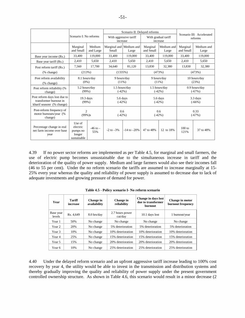
-51-

Scenario II: Delayed reforms Scenario I: No reforms With aggressive tariff

increase With gradual tariff

increase

Scenario III: Accelerated reforms

Marginal and Small

Medium and Large

Marginal and Small

Medium and Large

Marginal and Small

Medium and Large

Marginal and Small

Medium and Large

Base year income (Rs.) 33,400 119,000 33,400 119,000 33,400 119,000 33,400 119,000

Base year tariff (Rs.) 2,410 5,650 2,410 5,650 2,410 5,650 2,410 5,650

7,560 17,700 34,640 81,120 13,830 32,380 13,830 32,380 Post reform tariff (Rs.) (% change) (213%) (1335%) (473%) (473%)

Post reform availability (% change)

8.1 hours/day (0%)

9 hours/day (11%)

9 hours/day (11%)

10 hours/day (23%)

Post reform reliability (% change)

5.2 hours/day (99%)

1.5 hours/day (-42%)

1.5 hours/day (-42%)

0.9 hours/day (-67%)

Post reform days lost due to transformer burnout in

kharif seasonr (% change)

19.3 days (99%)

5.6 days (-42%)

5.6 days (-42%)

3.3 days (-66%)

Post-reform frequency of motor burnouts/year (%

change)

2 (99%)s

0.6 (-42%)

0.6 (-42%)

0.33 (-67%)

Percentage change in real net farm income over base

year

Use of electric

pumps no longer

sustainable

-46 to –55% -2 to –3% -14 to –20% 47 to 48% 12 to 18% 100 to

121% 37 to 48%

4.39 If no power sector reforms are implemented as per Table 4.5, for marginal and small farmers, the use of electric pump becomes unsustainable due to the simultaneous increase in tariff and the deterioration of the quality of power supply. Medium and large farmers would also see their incomes fall (46 to 55 per cent). Under the no reform scenario the tariffs are assumed to increase marginally at 15-25% every year whereas the quality and reliability of power supply is assumed to decrease due to lack of adequate investments and growing pressure of demand for power.

Table 4.5 - Policy scenario I- No reform scenario

Year Tariff increase

Change in availability

Change in reliability

Change in days lost due to transformer

burnout

Change in motor burnout frequency

Base year levels Rs. 4,649 8.0 hrs/day 2.7 hours power

cut/day 10.1 days lost 1 burnout/year

Year 1 50% No change No change No change No change Year 2 20% No change 5% deterioration 5% deterioration 5% deterioration Year 3 10% No change 10% deterioration 10% deterioration 10% deterioration Year 4 25% No change 15% deterioration 15% deterioration 15% deterioration Year 5 15% No change 20% deterioration 20% deterioration 20% deterioration

Year 6 10% No change 25% deterioration 25% deterioration 25% deterioration

4.40 Under the delayed reform scenario and an upfront aggressive tariff increase leading to 100% cost recovery by year 4, the utility would be able to invest in the transmission and distribution systems and thereby gradually improving the quality and reliability of power supply under the present government controlled ownership structure. As shown in Table 4.6, this scenario would result in a minor decrease (2

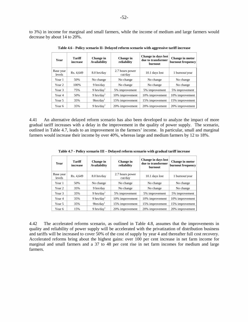
-52-

to 3%) in income for marginal and small farmers, while the income of medium and large farmers would decrease by about 14 to 20%.

Table 4.6 - Policy scenario II- Delayed reform scenario with aggressive tariff increase

Year Tariff increase

Change in Availability

Change in reliability

Change in days lost due to transformer

burnout

Change in motor burnout frequency

Base year levels Rs. 4,649 8.0 hrs/day 2.7 hours power

cut/day 10.1 days lost 1 burnout/year

Year 1 50% No change No change No change No change Year 2 100% 9 hrs/day No change No change No change Year 3 75% 9 hrs/day1 5% improvement 5% improvement 5% improvement Year 4 50% 9 hrs/day1 10% improvement 10% improvement 10% improvement Year 5 35% 9hrs/day1 15% improvement 15% improvement 15% improvement

Year 6 35% 9 hrs/day1 20% improvement 20% improvement 20% improvement

4.41 An alternative delayed reform scenario has also been developed to analyze the impact of more gradual tariff increases with a delay in the improvement in the quality of power supply. The scenario, outlined in Table 4.7, leads to an improvement in the farmers’ income. In particular, small and marginal farmers would increase their income by over 40%, whereas large and medium farmers by 12 to 18%.

Table 4.7 - Policy scenario III – Delayed reform scenario with gradual tariff increase

Year Tariff increase

Change in Availability

Change in reliability

Change in days lost due to transformer

burnout

Change in motor burnout frequency

Base year levels Rs. 4,649 8.0 hrs/day 2.7 hours power

cut/day 10.1 days lost 1 burnout/year

Year 1 50% No change No change No change No change Year 2 35% 9 hrs/day No change No change No change Year 3 35% 9 hrs/day1 5% improvement 5% improvement 5% improvement Year 4 35% 9 hrs/day1 10% improvement 10% improvement 10% improvement Year 5 35% 9hrs/day1 15% improvement 15% improvement 15% improvement Year 6 15% 9 hrs/day1 20% improvement 20% improvement 20% improvement

4.42 The accelerated reforms scenario, as outlined in Table 4.8, assumes that the improvements in quality and reliability of power supply will be accelerated with the privatization of distribution business and tariffs will be increased to cover 50% of the cost of supply by year 4 and thereafter full cost recovery. Accelerated reforms bring about the highest gains: over 100 per cent increase in net farm income for marginal and small farmers and a 37 to 48 per cent rise in net farm incomes for medium and large farmers.

-53-

Table 4.8 - Policy scenario III - Accelerated reform scenario

Year Tariff increase

Change in Availability

Change in reliability

Change in days lost due to transformer

burnout

Change in motor burnout frequency

Base year levels Rs. 4,649 8.0 hrs/day 2.7 hours power

cut/day 10.1 days lost 1 burnout/year

Year 1 50% No change No change No change No change Year 2 35% 9 hrs/day 25% improvement 25% improvement 25% improvement Year 3 35% 9 hrs/day1 20% improvement 25% improvement 20% improvement Year 4 35% 10 hrs/day1 20% improvement 25% improvement 20% improvement Year 5 35% 10 hrs/day1 20% improvement 25% improvement 20% improvement

Year 6 15% 10 hrs/day1 15% improvement 20% improvement 15% improvement

Notes: 1 Availability could increase considerably more, but since its effect is likely to diminish as hours available increase, only the reform scenario under 10 hours availability is considered

4.43 Marginal and small farmers, who account for more nearly two-thirds of all farmers in Haryana are most affected by these scenarios. According to the results, they could either face a significantly better life or farming with electric pumps would eventually become unsustainable for them.

K. Returns from Improvements in Reliability and Quality of Power Supply:

Comparison of Electric and Diesel Pumps 4.44 The policy simulations reported in the last section show the potential for large improvements in farm incomes if reforms are undertaken. An alternative way of cross-checking these results on gain from reforms is to compare the costs and returns associated with present day diesel and electric pump technology. Diesel pumps have close to 100% reliability, no problems associated with transformer burnouts and voltage fluctuations, and no problems of rationing in availability. However, the operating costs fo diesel pumps are much higher. Farmers also reported other problems such as problems in getting diesel, storing it and starting the diesel pump. Box 4.2 below summarizes some of the main differences between cost and return structure of electric and diesel pumps (Annex 6 section J describes these differences in detail). An econometric model was also developed to estimate the net income gain for electric pump owners if the reliability and quality of electricity supply is improved, all other things remaining constant, so as to make electric pumps comparable to diesel pumps (see Annex 6, section J for details on the model.)

4.45 The results of the analysis indicate that the average electric pump owner would gain round Rs. 82,000 in the short run if electricity power supply conditions (mainly reliability and quality of supply) are improved so as to mimic the conditions faced by diesel pump owners, but all other variables (including electricity tariffs) remain unchanged. Given the average current net income of electric pump owner of Rs.94,500, this premium for higher reliability and quality of supply represents a 87 per cent increase in net income in the short run for the average farmer. The effects could not be computed separately for small-marginal and medium-large farmers because of the small sample size of diesel pump owners. However, as shown earlier, it is likely that the effect would be much larger for small-marginal farmers and somewhat smaller for medium-large farmers63.

63 Also note that this estimate gives the short run effect. In the medium term, once irrigation technology adjusts, this effect is expected to be much larger.

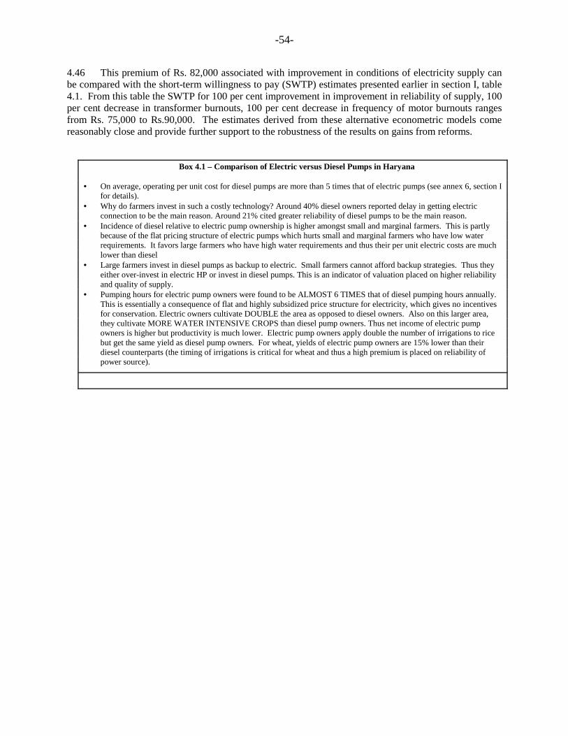
-54-

4.46 This premium of Rs. 82,000 associated with improvement in conditions of electricity supply can be compared with the short-term willingness to pay (SWTP) estimates presented earlier in section I, table 4.1. From this table the SWTP for 100 per cent improvement in improvement in reliability of supply, 100 per cent decrease in transformer burnouts, 100 per cent decrease in frequency of motor burnouts ranges from Rs. 75,000 to Rs.90,000. The estimates derived from these alternative econometric models come reasonably close and provide further support to the robustness of the results on gains from reforms.

Box 4.1 – Comparison of Electric versus Diesel Pumps in Haryana

• On average, operating per unit cost for diesel pumps are more than 5 times that of electric pumps (see annex 6, section I for details).

• Why do farmers invest in such a costly technology? Around 40% diesel owners reported delay in getting electric connection to be the main reason. Around 21% cited greater reliability of diesel pumps to be the main reason.

• Incidence of diesel relative to electric pump ownership is higher amongst small and marginal farmers. This is partly because of the flat pricing structure of electric pumps which hurts small and marginal farmers who have low water requirements. It favors large farmers who have high water requirements and thus their per unit electric costs are much lower than diesel

• Large farmers invest in diesel pumps as backup to electric. Small farmers cannot afford backup strategies. Thus they either over-invest in electric HP or invest in diesel pumps. This is an indicator of valuation placed on higher reliability and quality of supply.

• Pumping hours for electric pump owners were found to be ALMOST 6 TIMES that of diesel pumping hours annually. This is essentially a consequence of flat and highly subsidized price structure for electricity, which gives no incentives for conservation. Electric owners cultivate DOUBLE the area as opposed to diesel owners. Also on this larger area, they cultivate MORE WATER INTENSIVE CROPS than diesel pump owners. Thus net income of electric pump owners is higher but productivity is much lower. Electric pump owners apply double the number of irrigations to rice but get the same yield as diesel pump owners. For wheat, yields of electric pump owners are 15% lower than their diesel counterparts (the timing of irrigations is critical for wheat and thus a high premium is placed on reliability of power source).

-55-

CHAPTER 5

CONCLUSIONS AND RECOMMENDATIONS

A. Introduction 5.1 This chapter presents conclusions and recommendations in five areas: metering agriculture consumers, changing their tariff structure, raising electricity tariffs, adjusting canal water fees and it presents discussions on non-electricity specific complementary measures and an analysis of integrated demand side management programs.

B. Metering Agriculture Consumers 5.2 The lack of metering provides an incentive to utilities to camouflage non-technical losses (i.e. theft) under the estimated electricity consumption by agriculture consumers. This in turn, contributes to a lack of transparency in the operations of the utilities, a hidden inefficiency, and increasing financial losses. In Haryana, the metering study on a sample of farmers selected on the basis of a rigorous statistical analysis, indicates that in FY2000, the consumption by agriculture was about 2,876 GWh. The corresponding utility's estimate was Gwh 4,401 or 53 per cent higher. This would imply an overall level of transmission and distribution losses of 47 per cent compared to 37 per cent and equivalent to an additional financial burden for the utility of Rs.550 crores. While this estimate cannot be interpreted as a firm assessment of the electricity consumption by agriculture in Haryana, its order of magnitude is large enough to cast serious doubts on the accounts of the utilities. Regarding the acceptability of metering, according to the attitude survey in Haryana, the majority (69 per cent) of farmers who have a flat rate based power supply favor metered supply. 5.3 The benefits of Demand Side Management programs, will be effective and appreciated by farmers only when the use of electricity is metered and both costs and savings are measurable. 5.4 Metering of agriculture consumers is indispensable to quantify electricity consumption by agriculture and consequently to assess the level of system losses. Through metering, power utilities would be equipped with the necessary tool to plug commercial losses and benchmark their performance. Metering is also necessary for introducing appropriate price incentives for the efficient use of water drawn with electrical pumpsets and therefore for conservation of water and energy resources. 5.5 Traditionally, utilities have raised concerns regarding the acceptability of metering by farmers and the economic and financial via.bility to undertake universal metering, in view of the low density of consumers in the rural areas and the administrative costs related to metering, billing and collection. But research show that the metering program is undoubtedly an economic and financial sustainable investment. The economic and financial analyses presented in Annex 6 for Haryana, indicate that metering the present 283,000 flat rate agriculture consumers, at an initial investment of Rs. 1.4 Billion, would lead to net economic benefits (equivalent to the deadweight loss less the cost of meters) of about Rs.3.9 Billion. In financial terms, utilities would be able to gain more than Rs. 4 billion per annum on account of additional sales and purchase cost savings. 5.6 Apparently, the Government of Haryana has already decided to meter all new consumers, including agriculture consumers, though it is not clear whether the decision is being implemented and would be extended to all consumers. In Haryana, due to the favorable conditions of a relatively small number of tubewells to be metered and the greater accessibility in rural areas, the implementation of universal metering could take place over a two-year period.

-56-

C. Tariff Structure 5.7 The present tariff based on a flat rate structure is regressive, penalizing marginal and small farmers who are using less electricity for a given connected capacity. It also discourages farmers from conserving groundwater resources, as the marginal cost of pumping is zero. In an arid state like Haryana, water is a scarce resource and over-pumping in the long run will adversely affect agriculture. 5.8 Because the present tariff structure is based on the depth of the water table which varies during the year, it makes it impossible to make know exactly what to charge farmers. The flat rate tariff structure is also subjected to significant error. The utilities lose significant revenues because of equivalent under-reporting of HP. 5.9 The introduction of universal metering would allow utilities to charge agriculture consumers on the basis of the energy consumed and therefore remove the inequity associated with the present tariff regime. 5.10 Metering would also allow the Electricity Regulatory Commissions to devise methodologies and test different mechanisms for targeting subsidies more efficiently and effectively. For example, it could be possible to define "lifeline rates". A meter based tariff regime would also allow eliminating the present practice of declaring a lower installed horsepower capacity level by farmers. 5.11 A metered tariff would provide incentives for energy efficiency and thus for water conservation. Energy efficiency incentives would in turn allow for the introduction and implementation of end use efficiency initiatives, such as the replacement of old and inefficient pumpsets. 5.12 Recently, several State Electricity Regulatory Commissions64 have advocated or mandated the utilities to meter all tubewells and provided incentives to farmers to opt for meters through the provision of a lower metered tariff compared to the flat rate. However, more substantial financial incentives need to be introduced to facilitate the adoption of metered tariffs.

D. Raising Electricity Tariffs 5.13 The current tariff level for agriculture consumers in Haryana is inadequate to cover the cost of supply. As it represents only about 12 per cent of the embedded cost, it results in a significant burden on the finances of the utilities.

5.14 Raising electricity tariffs for agriculture is therefore essential for achieving the financial sustainability of electric (public and private) utilities. It is necessary to allow them to strengthen their capacity to undertake the needed investment to deliver adequate and reliable power to all consumers. And for the state as whole, increased cost recovery will reduce the fiscal subsidy required by the energy sector and thus help improve the overall fiscal health of the State to finance other productive investments, which due to fiscal constraints could not be supported. Utilities and governments can no longer support Rs 8 billion of annual subsidies to farmers, and the industrial sector can no longer cross subsidize them by Rs. 1.5 billion per year65.

5.15 Farmers are paying a higher price for electricity than stated by the utility because the poor quality of electricity supply increases the cost to farmers directly due to frequent pump motor burnouts and encourages them to adopt expensive coping strategies (such as additional diesel pump(s), larger capacity and more robust pumps) to deal with the erratic supply and quality of electricity. Poor power 64 See Tariff Orders of SERCs of Marahastra, Andhra Pradesh, Karnataka and Haryana itself. 65 The estimates are included in the Tariff Order of December 22 by the Haryana Electricity Regulatory Commission, section 6.3.5

-57-

supply conditions due to transformer burn outs and the long time required to repair them and other unscheduled power cuts, impose an additional cost to farmers due to the potential loss in crop yields. 5.16 Adopting measures to improve electricity supply conditions would increase the acceptability of power tariff increases. These could involve a number of technical measures such as reducing the number of days to complete transformer repair and improving the distribution infrastructure. For example, a tariff increase equivalent to the cost incurred by farmers for repairing their burnout motor would allow the utility to finance the investment required to improve the quality of power supply. This improvement would decrease farmers costs and therefore restore net income to their original levels. 5.17 The state should privatize the distribution companies to speed up the process of improving supply. A privatized distribution system would have greater incentives to limit theft and collect payments. The root cause of frequent transformer burn-outs is due to overloading as a result of unofficial connections or theft, imbalance in loads, lack of maintenance and protection. 5.18 Policy analysis demonstrated that farmers are demanding higher quality electricity supplies and are willing to pay. Increases though will have to come at a certain pace to that corresponds with an improvement in the service. But because of the highly politicized environment, the government and utilities will have to undertake information campaigns to ensure that the increases are understood. These campaigns could also inform users of a grace period to obtain official connections and the stiffer pre-announced penalties that would be levied on those who do not come forward.

E. Canal Water Pricing 5.19 The subsidized pricing of canal water puts electric pump owners at a disadvantage and does nothing to help conservation. Currently, water charges in Haryana cover only 49 per cent of the O&M costs (excluding interest and depreciation charges), of which 39 per cent is actually collected. 5.20 Over the short- to medium term, water prices should move towards full recovery of full operations and maintenance costs. This is in line with the on-going dialogue in the State to: (i) enable appropriate execution of O&M activities and thus ensure the longer term sustainability of surface irrigation systems; and (ii) eliminate the fiscal burden and contribute to the improved fiscal health in the State. It would also foster more efficient use of water in areas dependent on surface irrigation.

F. Complementary Measures to Improve Returns to Agricultural Production Activities

5.21 In the short to medium term, Haryana state should improve the delivery of agriculture support services and eliminate domestic restriction to trade by the Central and State government. This would improve the returns to agricultural production activities to enable full cost recovery of electricity tariffs and canal water prices. 5.22 In the short- to medium term, the state should invest in improving rural infrastructure such as all-weather rural roads, village markets, and telecommunications. These investments would significantly reduce the cost of marketing of both agricultural inputs (fertilizer, seeds, etc) and agricultural products. Poor infrastructure increases marketing costs due to associated higher physical losses (spoilage, spillage, wastage, etc) and bottlenecks (loading and transport) created in the system due to the inadequate capacity in meeting demand for marketing services. Such investments would in turn benefit both producers and consumers by reducing marketing margins, and translating to higher farm and lower consumer prices.

-58-

5.23 The state should increase efforts in the short to medium term to improve the delivery of public and private agricultural support services, particularly agricultural extension programs to increase the productivity of irrigated agriculture and to enhance farmer capabilities to diversify production to higher value crops. . For example, diversification to higher value crops and the adoption of improved agricultural technologies that would facilitate increased on-farm efficiency and productivity would enhance farm incomes and thus enable farmers absorb increasing electricity tariffs. Measures should include dissemination of improved technologies (such as higher yielding seeds, farm equipment, more efficient pumps), transferring knowledge to foster diversification to higher value crops and providing training on on-farm management practices, such as improved on-farm nutrient and water management, integrated pest management, and post-harvest practices. Government efforts could involve both improving public extension services as well as promoting the enabling environment for private delivery (including subcontracting to the private sector some activities). 5.24 Over the medium-term, the Government of India should lift various regulations related to marketing as this would improve marketing efficiency and would be critical to the longer term sustainability of power sector reform (See Box 5.1). These would include lifting controls on marketing activities, such as storage, movement, credit, export and import controls and the small-scale reservation of selected industries. At the state level, this would include phasing out the levy on rice mill output, currently at 75 per cent. Elimination of these controls will reduce transaction costs of marketing and hence allow better prices for farmers and consumers. They will also encourage greater private sector investments in marketing infrastructure (e.g. storage) that will reduce marketing losses. Improved electricity supply in rural areas would also facilitate growth of such industries. Progress in the reform of these restrictions, however, has been slow. The on-going WTO negotiations on agriculture is likely to necessitate some reform of domestic regulatory policies, thereby hastening the process. Collaborative efforts across states to move the reform process forward would be critical. 5.25 The State should not resort to offering higher commodity support prices to compensate farmers for the increase in power tariffs to agriculture for three key reasons. 5.26 First, the minimum support prices (MSP) are set by the Central Government, which in itself has created supply management problems for the GOI in terms of burgeoning buffer stocks and buffer stock cost. Should the Government of Haryana offer a support price higher the Central government MSP, the full cost of this price subsidy would have to be born by the Haryana budget. For example, In 1997/98, Haryana's rice and wheat production were 2.5 million mt and 7.6 million mt respectively (CMIE 1999). At an estimated marketed surplus of 73 per cent (Directorate of Economics and Statistics, GOI), this translates to about 7.4 million mt of grains that would be eligible for price support. Assuming the state government increases the support price by a mere 50 paise per kg over that of the GOI minimum support price for rice and wheat, this would at a minimum translate to a budgetary subsidy/cost of Rs 3.7 billion ($81 million) per year, equivalent to 0.01% of GSDP. This does not count the additional subsidy that would be required to cover the cost of storage and associated physical losses during storage. As illustrated by the high buffer stocking costs of the Government of India, such costs rise rapidly if the inventory is not sold quickly. These in turn could nullify much of the savings that may be generated from increased cost recovery achieved through increased power tariffs and impose an additional fiscal burden on an already precarious fiscal situation. 5.27 Second, enforcement of the higher support price would be extremely difficult. For example, currently the FCI and its designated Haryana State agencies are required to purchase at the support price whatever wheat or paddy is offered by farmers. Given that neighboring states (Rajasthan, Punjab, Uttar Pradesh) grow the same crops, the porous State borders would make it extremely difficult to stop "unofficial" inflows of grain from neighboring states that would be drawn by the higher offered prices.

-59-

The experience of the Maharashtra State Cotton Cooperative Grower's Marketing Federation's monopoly cotton procurement scheme, which offers higher cotton prices than that which prevails in the open market, shows that the fiscal subsidy burden increases rapidly in part due to difficulties in containing inflows of cotton from neighboring states (World Bank 1999c). Operating the necessary administrative system to enforce this policy would involve significant additional costs as well as open significant temptations for undesirable rent-seeking. 5.28 Third, disposal of the agricultural commodities could become a problem. As it is, the 1999 minimum support price for wheat in India is above world market prices, posing a major problem for the GOI in reducing its burgeoning buffer stocks through exports. A higher Haryana commodity support price could introduce similar or even more severe problems for the State.

G. Integrated Approaches to Energy Efficiency

5.29 There are several measures that would help improve the use of groundwater resources. Metering, as noted above, whether for surface irrigation or water extracted by electric pumps, would permit improved pricing of the water to better reflect its scarcity value. A further advancement of graduated tariff rates (higher per unit rates at higher consumption levels), could help deal with the "rebound effect", that is farmers will irrigate more area with improved electricity supply leading to groundwater resource degradation. 5.30 Regulating access to water through registration of wells and regulation of well depth, spacing and pump capacity could also help limit over use of water. These regulations, however, would be administratively difficult to enforce in India due to large number of small farmers. Equity is also an important concern, as registration would favor current pump owners vs new ones. 5.31 Organization of regional/local groundwater user groups could provide a mechanism for workable collective self-enforcement. The organization of community-based groundwater conservation districts is being piloted in Rajasthan and would provide useful lessons in the future. These could be complemented by information and education campaigns to generate greater awareness on the importance of sustainable groundwater use. 5.32 Pilot projects in Haryana have already demonstrated the benefits of Integrated Agricultural DSM (IADSM.), a program which consists of metering agriculture consumers, upgrading low voltage feeders to higher voltage and replacing irrigation pumps. The large scale implementation of such a project would get a demand push from farmers with the introduction of metered tariffs and tariff rationalization. The distribution system refurbishment, a prerequisite for DSM, would get stimulated with progressive increase in revenue for the utility from the agricultural consumers. The IADSM when implemented with metering and progressive rationalization of tariffs is a win win situation for the utility, farmer specially marginal and smaller, and the economy. The farmers would gain by improved quality and reliability of power supply, no motor burnings without much impact on their budgets. The utility would gain by lowering of costs towards electricity purchase, low failure rate of distribution transformers, increase in revenues and happy customers. The economic and financial analysis of IADSM for 15, 000 pumpsets program in Haryana is provided in the Box 5.2 below.

-60-

5.33 Water Supply side management. Important supply side initiatives could include the promotion of water conservation technologies in water short areas, such as water recharge structures, drip irrigation/sprinklers, and water recycling technologies. Fostering the adoption of these technologies is already currently being supported under watershed management and irrigation projects supported by the World Bank and other donors. Investments in drainage facilities are another option in waterlogged areas.

Box 5.2 - Economic and Financial Analysis of implementing Integrated Approaches to Efficiency

DSM benefits are particularly attractive in a peak deficit situation and more so in an energy and peak deficitsituation as in the Indian power sector. During the period of deficit, the economic benefit to the utilities throughIADSM would be equal to the WTP of HT customers. When the deficit in the sector is overcome, the economicbenefit would be equal to the avoided cost of new supply. Within this context, in an economic analysis of a proposed, 15,000 pumpset Agricultural DSM program in Haryana, thepower deficits were assumed to run up to 2008. The other economic benefits accrue to the farmers in the form ofeliminated rewind costs and delayed purchase of pumpsets. All benefits were assumed to start in year 2 ( the year afterconstruction) and last for the full life of the equipment (assumed to be 18 years). Economic costs include the installedcost of pumpsets, meters and Less LT system, (less taxes and adjusted), plus the maintenance costs borne first by theutility and then by the farmers over the 18 year life of the equipment.

Within this the reference case EIRR with the above assumptions was found to be 53 per cent with a total net

economic benefit (NPV) of Rs. 1,385 million. The cost of saved energy is 2.7 Rs/kWh. The economic returns appearto be robust to key parameters. Economic returns are always greater than 25 per cent even when contingencies of 30per cent are assumed, pmpset savings and LT loss reduction is lower, equipment life is only 10 years, and thewillingness to pay drops to 1.65 Rs.kWh.

The financial returns are less robust to key parameters than the economic returns, but still show excellent

returns under most circumstances. Only when revenue from the resale of savings drops below 2.0 Rs/kWh, or all of thekey parameters change, are the returns below the opportunity cost of capital. A tariff of 2.0 Rs/unit is, however, closeto the current average tariff in Haryana, showing how important the resale of saings to HT customers is to the viabilityof the program. Besides realized tariff, financial returns are most sensitive to pumpset savings and loss reduction. Lifeof equipment is only important if pumpset savings and loss reduction are lower than expected. This is because underthe reference case, most of the project benefits are achieved in the first 5-10 years.