Embed Size (px)
Citation preview

MODULATION FORMATS FOR
WAVELENGTH DIVISION MULTIPLEXING (WDM)
SYSTEMS
A THESIS SUBMITTED TO
THE GRADUATE SCHOOL OF NATURAL AND APPLIED SCIENCES
OF
MIDDLE EAST TECHNICAL UNIVERSITY
BY
F. FEZA BÜYÜKŞAHİN ÖNCEL
IN PARTIAL FULFILLMENT OF THE REQUIREMENTS
FOR
THE DEGREE OF DOCTOR OF PHILOSOPHY
IN
PHYSICS
SEPTEMBER 2009

Approval of the thesis:
MODULATION FORMATS FOR
WAVELENGTH DIVISION MULTIPLEXING (WDM) SYSTEMS
submitted by F. FEZA BÜYÜKŞAHİN ÖNCEL in partial fulfillment of the of the
requirements for the degree of Doctor of Philosophy in Physics Department,
Middle East Technical University by,
Prof. Dr. Canan Özgen _______________
Dean, Graduate School of Natural And Applied Sciences
Prof. Dr. Sinan Bilikmen _______________
Head of Department, Physics
Assoc. Prof. Dr. Serhat Çakır _______________
Supervisor, Physics Dept., METU
Examining Committee Members:
Prof. Dr. Sinan Bilikmen _______________
Physics Dept., METU
Assoc. Prof. Dr. Serhat Çakır _______________
Physics Dept., METU
Assist. Prof. Dr. Behzat Şahin _______________
Electrical and Electronics Engineering Dept., METU
Assoc. Prof. Dr. Akif Esendemir _______________
Physics Dept., METU
Assoc. Prof. Dr. Şemsettin Türköz _______________
Physics Dept., Ankara University
Date: _______________

iii
I hereby declare that all information in this document has been obtained and
presented in accordance with academic rules and ethical conduct. I also declare
that, as required by these rules and conduct, I have fully cited and referenced
all material and results that are not original to this work.
Name, Last name : F. Feza BÜYÜKŞAHİN ÖNCEL
Signature :

iv
ABSTRACT
MODULATION FORMATS FOR
WAVELENGTH DIVISION MULTIPLEXING (WDM) SYSTEMS
Büyükşahin Öncel, F. Feza
Ph.D, Department of Physics
Supervisor: Assoc. Prof. Dr. Serhat Çakır
September 2009, 159 pages
Optical communication networks are becoming the backbone of both national
and international telecommunication networks. With the progress of optical
communication systems, and the constraints brought by WDM transmissions and
increased bit rates, new ways to convert the binary data signal on the optical carrier
have been proposed.
There are different factors that should be considered for the right choice of
modulation format, such as information spectral density (ISD), power margin, and
tolerance against group-velocity dispersion (GVD) and against fiber nonlinear effects
like self-phase modulation (SPM), cross-phase modulation (XPM), four-wave
mixing (FWM), and stimulated Raman scattering (SRS).
In this dissertation, the several very important modulation formats such as
Non Return to Zero (NRZ), Return to Zero (RZ), Chirped Return to Zero (CRZ),
Carrier Suppressed Return to Zero (CSRZ), Differential Phase Shift Keying (PSK)
and Carrier Suppressed Return to Zero- Differential Phase Shift Keying (CSRZ-
DPSK) will be detailed and compared.
In order to make performance analysis of such modulation formats, the
simulation will be done by using VPItransmissionMakerTM
WDM software.
Keywords: Optical fiber communication, optical modulation, Wavelength
Division Multiplexing (WDM).

v
ÖZ
DALGA BOYU BÖLMELİ ÇOĞULLAMA (WDM) SİSTEMLERİ İÇİN
MODÜLASYON FORMATLARI
Büyükşahin Öncel, F. Feza
Doktora, Fizik Bölümü
Tez Yöneticisi: Doç. Dr. Serhat Çakır
Eylül 2009, 159 sayfa
Optik iletişim ağları hem ulusal hem de uluslararası iletişim ağlarının bel
kemiğini oluşturmaktadır. Optik iletişim sistemlerdeki gelişme, WDM iletimindeki
sınırlamalar ve artan bit oranları, optik taşıyıcı üzerindeki ikili veriyi çevirmede yeni
yollara gereksinim getirmektedir.
Modülasyon formatının seçiminde dikkat edilmesi gereken faktörler vardır.
Bilgi spektrumu yoğunluğu (ISD), güç payı, grup hız dağınımı (GVD) ve kendinden
kaymalı faz modülasyonu (SPM), karşı faz modülasyonu (XPM), dört-dalga karışımı
(FWM) ve uyarılmış Raman saçılımı (SRS), gibi lineer olmayan etkilere karşı direnç
dikkate alınmalıdır.
Bu tezde, önemli modülasyon formatlarından Non Return to Zero (NRZ),
Return to Zero (RZ), Chirped Return to Zero (CRZ), Carrier Suppressed Return to
Zero (CSRZ), Differential Phase Shift Keying (PSK) and Carrier Suppressed Return
to Zero- Differential Phase Shift Keying (CSRZ-DPSK) incelenerek, karşılaştırma
yapılacaktır.
WDM sistemlerinde, belirtilen modülasyon formatlarında performans analizi
yapmak için VPItransmissionMakerTM
WDM yazılımı kullanılarak simülasyon
yapılacaktır.
Anahtar Kelimeler: Fiber optik iletişim, optik modülasyon, Dalgaboyu
Bölmeli Çoğullama iletim sistemleri (WDM).

vi
ACKNOWLEDGMENTS
I would like to acknowledge gratefully to my supervisor Assoc. Prof. Dr.
Serhat Çakır for his guidance, support and encouragement during this dissertation.
I would also like to thank to Head of Department of Physics Prof. Dr. Sinan
Bilikmen for his financial support to buy simulation software.
I also wish to express my sincere appreciation to the other members of my
advisory committee, Assist. Prof. Dr. Behzat Şahin, Assoc. Prof Dr. Akif Esendemir
Assoc. Prof Dr. Şemsettin Türköz. I would like to thank Assist. Prof. Dr. Behzat
Şahin for his kindly helps, advice and guidance to use simulation software. I would
also like to thank Assoc. Prof. Dr. Akif Esendemir for his encouragement.
I am also grateful to my friend, Halil for his help, support and suggestions.
Finally, I want to thank to my parents, my sister Ayda, my brother Ufuk and
my husband Ömer for their supports and encouragements. To them, I dedicate this
dissertation.

vii
TABLE OF CONTENTS
ABSTRACT ................................................................................................................ iv
ÖZ ................................................................................................................................ v
ACKNOWLEDGMENTS .......................................................................................... vi
TABLE OF CONTENTS ........................................................................................... vii
CHAPTERS
1. WDM SYSTEMS ............................................................................................... 1
1.1 INTRODUCTION ....................................................................................... 1
1.2 TRANSMISSION IMPAIRMENTS ............................................................ 3
1.2.1 Linear Effects ..................................................................................... 3
1.2.1.1 Fiber Attenuation ................................................................. 3
1.2.1.2 Amplified Spontaneous Emission Noise (ASE) .................. 6
1.2.1.3 Dispersion ............................................................................ 7
1.2.1.3.1 Material Dispersion ................................................... 8
1.2.1.3.2 Waveguide Dispersion ............................................... 8
1.2.1.3.3 Modal Dispersion..................................................... 10
1.2.2 Nonlinear Effects ............................................................................. 11
1.2.2.1 Stimulated Brillouin Scattering (SBS) .............................. 11
1.2.2.2 Stimulated Raman Scattering (SRS) ................................. 11
1.2.2.3 Self-Phase Modulation (SPM) ........................................... 12
1.2.2.4 Cross Phase Modulation (XPM) ........................................ 13
1.2.2.5 Four Wave Mixing (FWM) ............................................... 13
2. MODULATION FORMATS IN WDM SYSTEMS ........................................ 14
2.1 INTRODUCTION ..................................................................................... 14
2.2 OPTICAL MODULATOR ........................................................................ 15
2.2.1 Direct Modulation ............................................................................ 15
2.2.2 External Modulation......................................................................... 16

viii
2.3 MODULATION FORMATS ..................................................................... 17
2.3.1 Non Return To Zero (NRZ) ............................................................. 19
2.3.2 Return To Zero (RZ) ........................................................................ 21
2.3.2.1 Chirped RZ (CRZ) ............................................................. 25
2.3.2.2 Carrier Suppressed RZ (CSRZ) ......................................... 26
2.3.3 Differential Phase Shift Key (DPSK) .............................................. 29
2.3.3.1 Non Return To Zero DPSK (NRZ-DPSK) ........................ 30
2.3.3.2 Return To Zero DPSK (RZ-DPSK) ................................... 32
2.3.3.3 Carrier Suppressed RZ-DPSK (CSRZ-DPSK) .................. 33
3. SIMULATIONS FOR MODULATION FORMATS ...................................... 35
3.1 SIMULATION MODEL ............................................................................ 35
3.2 PERFORMANCE ANALYSIS .................................................................. 37
3.3 40GB/S WDM SYSTEM ............................................................................ 41
3.3.1 Single Channel 40Gb/s WDM System ............................................. 41
3.3.1.1 NRZ Format ...................................................................... 41
3.3.1.2 RZ Format ......................................................................... 44
3.3.1.3 CRZ Format ....................................................................... 47
3.3.1.4 CSRZ Format .................................................................... 49
3.3.1.5 DPSK Format ................................................................... 51
3.3.1.6 CSRZ-DPSK Format ......................................................... 53
3.3.2 25 Channels 40Gb/s WDM System ................................................. 57
3.3.2.1 25 Channels NRZ Format .................................................. 57
3.3.2.2 25 Channels RZ Format .................................................... 60
3.3.2.3 25 Channels CRZ Format .................................................. 62
3.3.2.4 25 Channels CSRZ Format ................................................ 65
3.3.2.5 25 Channels DPSK Format ............................................... 67
3.3.2.6 25 Channels CSRZ DPSK Format .................................... 70
3.4 100 GB/S WDM SYSTEM ......................................................................... 74
3.3.1 Single Channel 100Gb/s WDM System ........................................... 74
3.3.1.1 NRZ Format ...................................................................... 75
3.3.1.2 RZ Format ......................................................................... 77
3.3.1.3 CRZ Format ....................................................................... 80

ix
3.3.1.4 CSRZ Format .................................................................... 83
3.3.1.5 DPSK Format .................................................................... 86
3.3.1.6 CSRZ DPSK Format ......................................................... 89
3.3.2 11 Channels 100Gb/s WDM System ............................................... 94
3.3.2.1 NRZ Format ...................................................................... 95
3.3.2.2 RZ Format ......................................................................... 97
3.3.2.3 CRZ Format ..................................................................... 100
3.3.2.4 CSRZ Format .................................................................. 103
3.3.2.5 DPSK Format .................................................................. 106
3.3.2.6 CSRZ DPSK Format ....................................................... 109
4. CONCLUSION ............................................................................................ 117
REFERENCES ......................................................................................................... 121
APPENDIX A .......................................................................................................... 124
CURRICULUM VITAE .......................................................................................... 139
x
LIST OF TABLES
TABLES
Table 3.1 Parameters of transmission fiber and dispersion compensating fiber at
1550nm. ...................................................................................................................... 35
Table 3. 2 Performance of 40 Gb/s and 100Gb/s WDM Systems with all Modulation
Formats and Compensating Configuration. ............................................................. 115

xi
LIST OF FIGURES
FIGURES
Figure 1.1 Implementation of typical WDM link [4]. .................................................. 3
Figure 1.2 Loss Spectrum of single mode fiber [2]. .................................................... 6
Figure 1.3 Loss and dispersion of dry fiber [2]. ........................................................... 6
Figure 1.4 Limitation of dispersion on information capacity [9]. ................................ 7
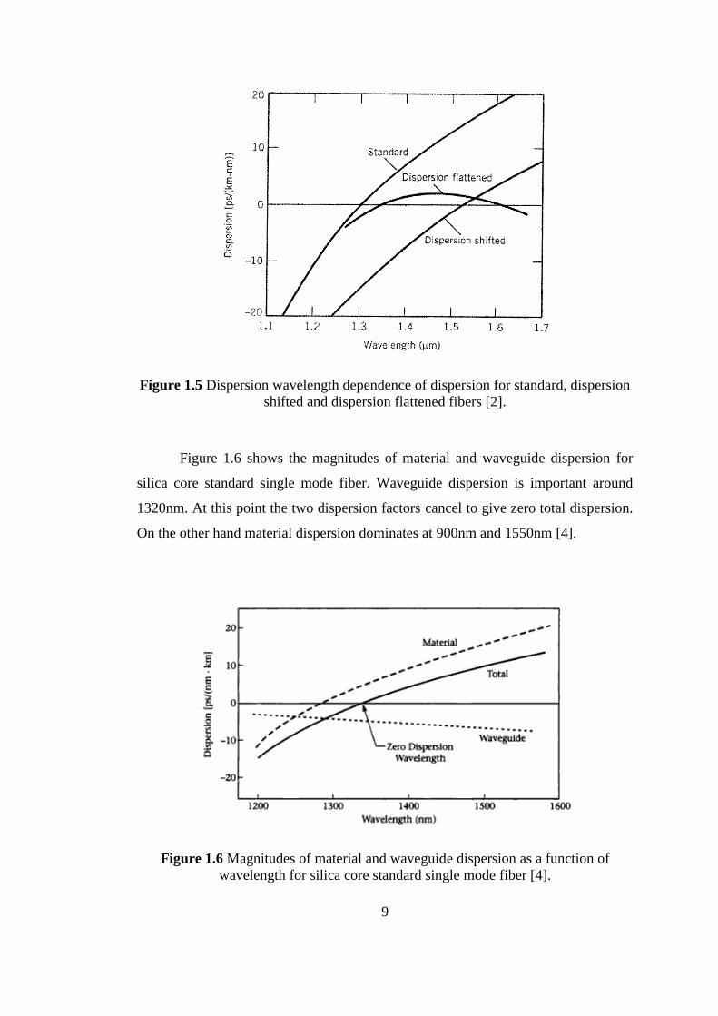
Figure 1.5 Dispersion wavelength dependence of dispersion for standard, dispersion
shifted and dispersion flattened fibers [2]. ................................................................... 9
Figure 1.6 Magnitudes of material and waveguide dispersion as a function of
wavelength for silica core standard single mode fiber [4]. .......................................... 9
Figure 2.1 Optical intensity modulator based on Mach- Zehnder interferometric
structure [15]. ............................................................................................................. 17
Figure 2.2 Representation of the NRZ code [19]. ...................................................... 19
Figure 2.3 NRZ transmitter diagram [13]. ................................................................. 19
Figure 2.4 The optical spectrum and waveform of 10Gb/s NRZ modulation
(simulated by VPItransmissionMakerTM
WDM and its simulation setup is shown in
Figure A.1 at Appendix A). ....................................................................................... 20
Figure 2.5 Representation of the RZ code [19]. ......................................................... 21
Figure 2.6 RZ transmitter [13]. .................................................................................. 21
Figure 2.7 The optical spectrum and waveform of 10Gb/s RZ (simulated by
VPItransmissionMakerTM
WDM and its simulation setup is shown in Figure A.2 at
Appendix A). .............................................................................................................. 22
Figure 2.8 Bandwidth of NRZ and RZ [6]. ................................................................ 23
Figure 2.9 Optical Spectrum and waveform of 10Gb/s RZ and NRZ (simulated by
VPItransmissionMakerTM
WDM). ............................................................................. 24
Figure 2.10 Chirped RZ transmitter [20]. .................................................................. 25

xii
Figure 2.11 The optical spectrum and waveform of 10Gb/s CRZ (simulated by
VPItransmissionMakerTM
WDM and its simulation setup is shown in Figure A.3 at
Appendix A). .............................................................................................................. 26
Figure 2. 12 Block diagram of CSRZ transmitter [17]. ............................................. 27
Figure 2.13 The optical spectrum and waveform of 10Gb/s CSRZ (simulated by
VPItransmissionMakerTM
WDM and its simulation setup is shown in Figure A.4 at
Appendix A). .............................................................................................................. 28
Figure 2.14 The optical spectrum and waveform of 10Gb/s DPSK (simulated by
VPItransmissionMakerTM
WDM and its simulation setup is shown in Figure A.5 at
Appendix A) ............................................................................................................... 30
Figure 2.15 Block diagrams of NRZ-DPSK transceiver and receiver [21]. .............. 31
Figure 2.16 Block diagram of RZ-DPSK transmitter [21]. ........................................ 33
Figure 2.17 The optical spectrum and waveform of 10Gb/s CSRZ DPSK (simulated
by VPItransmissionMakerTM
WDM and its simulation setup is shown in Figure A. 6
at Appendix A) ........................................................................................................... 34
Figure 3. 1 Configurations of the pre-, post-, and symmetrical compensation. ......... 36
Figure 3.2 General configuration of eye diagram. ..................................................... 38
Figure 3.3 Simplified eye diagram. ............................................................................ 38
Figure 3.4 Misinterpret transmitted digital data caused by jitter [25]. ...................... 39
Figure 3.5 BER versus Length with all dispersion compensating configuration. ...... 42
Figure 3.6 Eye diagrams of system for different fiber lengths. ................................. 43
Figure 3.7 BER versus Length with all dispersion compensating configuration. ...... 45
Figure 3.8 Eye diagrams of system for different fiber lengths. ................................. 46
Figure 3. 9 BER versus Length with all dispersion compensating configuration. ..... 47
Figure 3.10 Eye diagrams of system for different fiber lengths. ............................... 48
Figure 3. 11 BER versus Length with all dispersion compensating configuration. ... 49
Figure 3.12 Eye diagrams of system for different fiber lengths. ............................... 50
Figure 3.13 BER versus Length with all dispersion compensating configuration. .... 51
Figure 3.14 Eye diagrams of system for different fiber lengths. ............................... 52
Figure 3.15 BER versus Length with all dispersion compensating configuration. .... 53
Figure 3.16 Eye diagrams of system for different fiber lengths. ............................... 54
xiii
Figure 3.17 BER versus Length for single channel 40Gb/s system for all modulation
formats with pre-compensating configuration. .......................................................... 55
Figure 3.18 BER versus Length for single channel 40Gb/s system for all modulation
formats with post-compensating configuration. ......................................................... 56
Figure 3.19 BER versus Length for single channel 40Gb/s system for all modulation
formats with symmetrical compensating configuration. ............................................ 56
Figure 3.20 BER versus Length with all dispersion compensating configuration. .... 58
Figure 3.21 Eye diagrams of system for different fiber lengths. ............................... 59
Figure 3.22 BER versus Length with all dispersion compensating configuration. .... 60
Figure 3.23 Eye diagrams of system for different fiber lengths. ............................... 61
Figure 3.24 BER versus Length with all dispersion compensating configuration. .... 63
Figure 3.25 Eye diagrams of system for different fiber lengths. ............................... 64
Figure 3.26 BER versus Length with all dispersion compensating configuration. .... 65
Figure 3. 27 Eye diagrams of system for different fiber lengths. .............................. 66
Figure 3.28 BER versus Length with all dispersion compensating configuration. .... 68
Figure 3.29 Eye diagrams of system for different fiber lengths. ............................... 69
Figure 3.30 BER versus Length with all dispersion compensating configuration. .... 70
Figure 3.31 Eye diagrams of system for different fiber lengths. ............................... 71
Figure 3.32 BER versus Length for 25 channels 40Gb/s system for all modulation
formats with pre-compensating configuration. .......................................................... 72
Figure 3.33 BER versus Length for 25 channels 40Gb/s system for all modulation
formats with post-compensating configuration. ......................................................... 73
Figure 3.34 BER versus Length for 25 channels 40Gb/s system for all modulation
formats with symmetrical compensating configuration. ............................................ 74
Figure 3.35 BER versus Length with all dispersion compensating configuration. .... 75
Figure 3.36 Eye diagrams of system for different fiber lengths; (a) Pre-compensating
configuration, (b) Post-compensating configuration, (c) Symmetrical compensating
configuration. ............................................................................................................. 76
Figure 3.37 BER versus Length with all dispersion compensating configuration. .... 78
Figure 3.38 Eye diagrams of system for different fiber lengths; (a) Pre-compensating
configuration, (b) Post-compensating configuration, (c) Symmetrical compensating
configuration. ............................................................................................................. 79
xiv
Figure 3.39 BER versus Length with all dispersion compensating configuration. .... 81
Figure 3.40 Eye diagrams of system for different fiber lengths; (a) Pre-compensating
configuration, (b) Post-compensating configuration, (c) Symmetrical compensating
configuration. ............................................................................................................. 82
Figure 3.41 BER versus Length with all dispersion compensating configuration. .... 84
Figure 3.42 Eye diagrams of system for different fiber lengths; (a) Pre-compensating
configuration, (b) Post-compensating configuration, (c) Symmetrical compensating
configuration. ............................................................................................................. 85
Figure 3.43 BER versus Length with all dispersion compensating configuration. .... 87
Figure 3.44 Eye diagrams of system for different fiber lengths; (a) Pre-compensating
configuration, (b) Post-compensating configuration, (c) Symmetrical compensating
configuration. ............................................................................................................. 88
Figure 3.45 BER versus Length with all dispersion compensating configuration. .... 90
Figure 3.46 Eye diagrams of system for different fiber lengths; (a) Pre-compensating
configuration, (b) Post-compensating configuration, (c) Symmetrical compensating
configuration. ............................................................................................................. 91
Figure 3.47 BER versus Length for single channel 100Gb/s system for all modulation
formats with pre-compensating configuration. .......................................................... 92
Figure 3.48 BER versus Length for single channel 100Gb/s system for all modulation
formats with post-compensating configuration. ......................................................... 93
Figure 3.49 BER versus Length for single channel 100Gb/s system for all modulation
formats with symmetrical compensating configuration. ............................................ 94
Figure 3.50 BER versus Length with all dispersion compensating configuration. .... 95
Figure 3.51 Eye diagrams of system for different fiber lengths; (a) Pre-compensating
configuration, (b) Post-compensating configuration, (c) Symmetrical compensating
configuration. ............................................................................................................. 96
Figure 3.52 BER versus Length with all dispersion compensating configuration. .... 98
Figure 3.53 Eye diagrams of system for different fiber lengths; (a) Pre-compensating
configuration, (b) Post-compensating configuration, (c) Symmetrical compensating
configuration. ............................................................................................................. 99
Figure 3.54 BER versus Length with all dispersion compensating configuration. .. 101

xv
Figure 3.55 Eye diagrams of system for different fiber lengths; (a) Pre-compensating
configuration, (b) Post-compensating configuration, (c) Symmetrical compensating
configuration. ........................................................................................................... 102
Figure 3. 56 BER versus Length with all dispersion compensating configuration. . 104
Figure 3.57 Eye diagrams of system for different fiber lengths; (a) Pre-compensating
configuration, (b) Post-compensating configuration, (c) Symmetrical compensating
configuration. ........................................................................................................... 105
Figure 3.58 BER versus Length with all dispersion compensating configuration. .. 107
Figure 3.59 Eye diagrams of system for different fiber lengths; (a) Pre-compensating
configuration, (b) Post-compensating configuration, (c) Symmetrical compensating
configuration. ........................................................................................................... 108
Figure 3. 60 BER versus Length with all dispersion compensating configuration. . 110
Figure 3.61 Eye diagrams of system for different fiber lengths; (a) Pre-compensating
configuration, (b) Post-compensating configuration, (c) Symmetrical compensating
configuration. ........................................................................................................... 111
Figure 3.62 BER versus Length for 11 channels 100Gb/s system for all modulation
formats with pre-compensating configuration. ........................................................ 112
Figure 3.63 BER versus Length for 11channels 100Gb/s system for all modulation
formats with post-compensating configuration. ....................................................... 113
Figure 3.64 BER versus Length for 11 channels 100Gb/s system for all modulation
formats with symmetrical compensating configuration. .......................................... 114
Figure A.1 Simulation set up of 10 Gb/s NRZ modulation. .................................... 124
Figure A.2 Simulation set up of 10 Gb/s RZ modulation. ....................................... 124
Figure A.3 Simulation set up of 10 Gb/s CRZ modulation. .................................... 125
Figure A.4 Simulation set up of 10 Gb/s CSRZ modulation. .................................. 125
Figure A.5 Simulation set up of 10 Gb/s DPSK modulation. .................................. 126
Figure A. 6 Simulation set up of 10 Gb/s CSRZ DPSK modulation. ...................... 126
Figure A.7 Simulation set up of single channel 40 Gb/s NRZ (a) pre-compensating
configuration, (b) post-compensating configuration, (c) symmetrical compensating
configuration. ........................................................................................................... 127

xvi
Figure A.8 Simulation set up of single channel 40Gb/s RZ (a) pre-compensating
configuration, (b) post-compensating configuration, (c) symmetrical compensating
configuration. ........................................................................................................... 128
Figure A.9 Simulation set up of single channel 40Gb/s CRZ (a) pre-compensating
configuration, (b) post-compensating configuration, (c) symmetrical compensating
configuration. ........................................................................................................... 129
Figure A.10 Simulation set up of single channel 40Gb/s CSRZ (a) pre-compensating
configuration, (b) post-compensating configuration, (c) symmetrical compensating
configuration. ........................................................................................................... 130
Figure A.11 Simulation set up of single channel 40Gb/s DPSK (a) pre-compensating
configuration, (b) post-compensating configuration, (c) symmetrical compensating
configuration. ........................................................................................................... 131
Figure A. 12 Simulation set up of single channel 40Gb/s CSRZ-DPSK (a) pre-
compensating configuration, (b) post-compensating configuration, (c) symmetrical
compensating configuration. .................................................................................... 132
Figure A.13 Simulation set up of 25 channels 40Gb/s NRZ (a) pre-compensating
configuration, (b) post-compensating configuration, (c) symmetrical compensating
configuration. ........................................................................................................... 133
Figure A.14 Simulation set up of 25 channels 40Gb/s RZ (a) pre-compensating
configuration, (b) post-compensating configuration, (c) symmetrical compensating
configuration. ........................................................................................................... 134
Figure A.15 Simulation set up of 25 channels 40Gb/s CRZ (a) pre-compensating
configuration, (b) post-compensating configuration, (c) symmetrical compensating
configuration. ........................................................................................................... 135
Figure A.16 Simulation set up of 25 channels 40Gb/s CSRZ (a) pre-compensating
configuration, (b) post-compensating configuration, (c) symmetrical compensating
configuration. ........................................................................................................... 136
Figure A. 17 Simulation set up of 25 channels 40Gb/s DPSK (a) pre-compensating
configuration, (b) post-compensating configuration, (c) symmetrical compensating
configuration. ........................................................................................................... 137

xvii
Figure A. 18 Simulation set up of 25 channels 40Gb/s CSRZ-DPSK (a) pre-
compensating configuration, (b) post-compensating configuration, (c) symmetrical
compensating configuration. .................................................................................... 138

xviii
LIST OF ABBREVIATIONS
ASE Amplified Spontaneous Emission Noise.
ASK Amplitude Shift Keying.
BER Bit Error Rate.
CD Chromatic Dispersion.
CPFSK Continuous Phase Frequency Shift Keying.
CRZ Chirped Return to Zero.
CSRZ DPSK Carrier Suppressed Return to Zero Differential Phase Shift Key.
CSRZ Carrier Suppressed Return to Zero.
CWDM Coarse wavelength division multiplexing.
DCF Dispersion Compensating Fiber.
DMS-RZ Dispersion-Managed Soliton-Based Return to Zero.
DPSK Differential Phase Shift Key.
DQPSK Quaternary Phase Shift Keying.
DWDM Dense Wavelength Division Multiplexing.
EAM Electro-Absorption Modulator.
EDFA Erbium-Doped Fiber Amplifiers.
EOM Electro-Optic Modulators.
FEC Forward Error Correction.
FSK Frequency Shift Keying.
FWM Four Wave Mixing.
GVD Group-Velocity Dispersion.
IM/DD Intensity Modulated-Direct Detection.
ISD Information Spectral Density.
ISI Intersymbol Interference
ITU International Telecommunication Union.
MSK Minimum Shift Keying.
MZIM Mach-Zehnder Interferometer.
NF Noise Figure.

xix
NRZ DPSK Non Return to Zero Differential Phase Shift Key.
NRZ Non Return to Zero.
OOK On-Off Keying.
PMD Polarization Mode Dispersion.
PolSK Polarization Shift Keying.
PSK Phase Shift Keying.
RZ DPSK Return to Zero Differential Phase Shift Key.
RZ Return to Zero.
SBS Stimulated Brillouin Scattering.
SMF Single Mode Fiber.
SOP State of Polarization.
SPM Self-Phase Modulation.
SRS Stimulated Raman Scattering.
SSMF Standard Single Mode Fiber.
VSB-RZ Vestigial sideband Return to Zero.
WDM Wavelength Division Multiplexing.
XPM Cross Phase Modulation.

1
CHAPTER 1
WDM SYSTEMS
1.1 INTRODUCTION
Communication systems can be defined as the transfer of information from
one point to another. The information transfer is frequently achieved by
superimposing or modulating the information on to an electromagnetic wave acting
as a carrier for the information signal. This modulated carrier is then transmitted to
the required destination where it is received and the original information signal is
obtained by demodulation. Electromagnetic carrier wave can operate at radio
frequencies, microwave frequencies, millimeter wave frequencies and optical range
of frequencies [1]. Optical communication systems also called lightwave systems use
carrier frequencies in the visible or near infrared region of the electromagnetic
spectrum. Fiber optic communication systems are lightwave systems where the
information is transmitted through the optical fiber [2]. In recent years, fiber optic
communication systems become a most desirable communication system because of
the present and the future demand for combined voice, video and data transmission,
high-speed Internet access, multimedia broadcast systems, high-capacity data
networking for grid computing and remote storage.
The tremendous growth in demand for bandwidth has led to various
technologies to increase the capacity. The use of wavelength-division multiplexing
(WDM) technology, which supports multiple simultaneous channels on a single
fiber, offers a further boost in fiber transmission capacity. WDM transmission
systems with transmission capacity exceeding a Tera-bit per second are becoming
commercially available. Two different versions of WDM, defined by standards of
the International Telecommunication Union (ITU), are distinguished: Coarse
wavelength division multiplexing (CWDM) uses a relatively small number of
channels (four or eight), and a large channel spacing of 20 nm. The nominal

2
wavelengths range from 1310 nm to 1610 nm. The single channel bit rate is usually
between 1 and 3.125 Gb/s. Dense wavelength division multiplexing (DWDM)
enhance the total transmission capacity by increasing the number of multiplexed
channels. It uses large number of channels (40, 80, or 160), and a correspondingly
small channel spacing of 12.5GHz (0.1nm), 25 GHz (0.2nm), 50 GHz (0.4nm) or
100 GHz (0.8nm). All optical channel frequencies refer to a reference frequency of
193.10 THz (1552.5 nm). The single-channel bit rate can be 10 Gb/s, 20Gb/s, 40Gb/s
and also 100 Gb/s [3].
Figure 1.1 shows the implementation of typical WDM link. At the
transmitting end there are several independently modulated light sources, each
emitting signals at a unique wavelength. To combine these optical outputs into a
continuous spectrum of signals and couple them onto a single fiber, a multiplexer is
needed. To separate the optical signals into appropriate detection channels for signal
processing a demultiplexer is required at the receiving end. The fiber losses are
compensated for using the amplifier. Optical amplifiers are divided into three
categories in terms of the function they perform such as boosters or a post-amplifier,
in-line amplifiers, and preamplifiers. A post-amplifier is placed immediately after a
transmitter. A post-amplifier magnifies a signal before sending it down a fiber. Its
main function is to produce maximum optical power. An in-line amplifier is placed
in the middle of a fiber optic link to compensate for power losses caused by fiber
attenuation, connections, and signal distribution in networks. The number of in-line
amplifiers needed depends on the length of the fiber-optic link and the network‟s
configuration. For long-haul links, in-line amplifiers are usually installed every 80 to
100 km. These amplifiers compensate for losses caused by fiber attenuation and
splices. They are also needed for short-distance networks to compensate for losses
caused by signal distribution in a local area network. A preamplifier magnifies a
signal immediately before it reaches the receiver [4].

3
Figure 1.1 Implementation of typical WDM link [4].
1.2 TRANSMISSION IMPAIRMENTS
There are several factors that seriously degrade the WDM system
performance. When an optical signal transmits over a fiber, it suffers from linear and
nonlinear degrading effects in the fiber. Optical loss or attenuation, amplified
spontaneous emission noise (ASE), polarization mode dispersion (PMD), and
chromatic dispersion (CD) are linear degrading effects; Stimulated Raman scattering
(SRS), stimulated Brillouin scattering (SBS) and Kerr effect are nonlinear degrading
effects. The effects of self-phase modulation (SPM), cross-phase modulation (XPM)
and four-wave mixing (FWM), due to Kerr effect, and stimulated Raman scattering
(SRS) effects arise from the interaction two or more channels, so these effects are
particular concern in WDM systems [5]. In order to understand the requirements on
the modulation formats, it is important to know the limitations of optical
communication systems. Therefore, in this dissertation the various phenomena that
limit the transmission reach will be described.
1.2.1 Linear Effects
1.2.1.1 Fiber Attenuation
Attenuation is the most fundamental impairments that affect signal
propagation and limit transmission distance in fiber. It is given as a specification for

4
a particular fiber type. Attenuation is a property of the fiber, and it is result of the
various material, structural, and modular impairments in a fiber [6].
When optical signal is transmitted over fiber, its power is lost and its
amplitude is reduced. This amplitude reduction or attenuation coefficient α is
expressed in dB/km.
Power attenuation inside an optical fiber is governed by Beer‟s Law.
(1.1)
In Eq. (1.1) is the change in power with respect to length and α is the
attenuation coefficient. If Pin is the input optical power (W), Pout is the output optical
power (W) and L (km) is the total length of the fiber, we can express the output
power Pout as the following equation.
(1.2)
The attenuation constant α can be written in common units of dB/km. Decibel
is defined in terms of the logarithm of a power or intensity ratio. by using following
relation
(1.3)
and it is referred as fiber loss.
Thanks to the progress of fiber manufacturing, the attenuation of fibers has
gone down to slightly below 0.2 dB/km at 1.55 μm where the attenuation is nearly
minimum [2][6].
Material absorption and Rayleigh scattering are most important factors that
cause a fiber loss. Optical fiber absorption is material specific and can be divided
into two categories: intrinsic absorption and extrinsic absorption. Intrinsic absorption
results from the interaction of free electrons and the operating wavelength within the
fiber material. Extrinsic absorption results from the presence of the impurities. The

5
metal ions are most undesirable impurities in an optical fiber. Rayleigh scattering
arises from microscopic variations in the material density, from compositional
fluctuations and from structural inhomogenities. Rayleigh scattering causes a small
part of the optical ray to escape from its path thus, causing small attenuation [7].
Attenuation depends on the wavelength of transmitted light. Figure 1.2 shows
the loss spectrum of a single mode fiber. Attenuation at 1.55μm is only 0.2 dB/km,
the lowest value first realized in 1979. This value is close to the limit of the silica
fibers about 0.16dB/km. Attenuation has strong peak near 1.39μm and minimum
peak near 1.3μm where the attenuation is below 0.5dB/km. this low-loss window was
used for second-generation lightwave systems. For shorter wavelengths attenuation is
higher exceed 5dB/km in the visible region and this wavelengths are not suitable for
long-haul transmission. The material absorption and Rayleigh scattering are also
shown in this figure. The intrinsic material absorption for silica in the wavelength
range 0.8-1.6μm is below 0.1dB/km as shown in this figure. In fact, it is less than
0.03dB/km in the 1.3μm to 1.6μm wavelength range which are commonly used for
lightwave systems. The main source of extrinsic absorption in silica fiber is the
presence of water vapors. Its harmonic and combination tones with silica produce
absorption at the 1.39μm, 1.24μm and 0.95μm wavelengths. In dry fiber, the OH ion
concentration is reduced to low levels that the 1.39μm peak almost disappears as
shown in Figure 1.3. Any wavelength below 0.8μm is unusable for optical
communication because Rayleigh scattering is high. In addition propagation above
the 1.7μm is not possible because of high losses from infrared absorption [2].

6
Figure 1.2 Loss Spectrum of single mode fiber [2].
Figure 1.3 Loss and dispersion of dry fiber [2].
1.2.1.2 Amplified Spontaneous Emission Noise (ASE)
Amplified spontaneous emission (ASE) is the dominant noise generated in an
optical amplifier. The spontaneous recombination of electrons and holes in the
amplifier medium cause an ASE. Due to nonlinear interaction between the amplified
spontaneous emission (ASE) noise from optical amplifiers and the signal, the ASE
noise is being amplified by the signal during propagation.

7
The amount of noise generated by the amplifier depends on factors such as
the amplifier gain spectrum, the noise bandwidth, and the population inversion
parameter, which specifies the degree of population inversion that has been achieved
between two energy levels. If multiple optical amplifiers are cascaded to periodically
compensate for fiber loss, ASE builds up in the system. Each subsequent amplifier in
the cascade amplifies the noise generated by previous amplifiers.
Optical amplifiers based on erbium-doped fibers are now widely deployed
within terrestrial and submarine systems. They provide high gain, large optical
bandwidth, and low-noise figure (NF), and several tens of erbium-doped fiber
amplifiers (EDFA) can be cascaded [3][8].
1.2.1.3 Dispersion
Dispersion is the broadening of the signal pulse while through the fiber.
Figure 1.4 shows how dispersion limits the information capacity. Dispersion cause
pulses to spread in time. When pulses arrive at the output, they have broadened.
Figure 1.4 Limitation of dispersion on information capacity [9].
There are three types of dispersion in waveguides: material dispersion,
waveguide dispersion and modal dispersion.

8
1.2.1.3.1 Material Dispersion
In material dispersion, different wavelengths of light travel at different
velocities within a medium. In a dispersive medium pulse spread out in time and
space .
The index of refraction is the most widely used parameter for waveguide
design. Material dispersion occurs because of the variation of index of refraction as a
function of the optical wavelength [4][9]. The refractive index, n (w), is estimated by
the Sellmeier equation (Eq.(1.4)). Material dispersion is proportional to the
differential of the group index.
(1.4)
where wj is the resonance frequency and Bj is the oscillator strength [6].
1.2.1.3.2 Waveguide Dispersion
Waveguide dispersion is similar to material dispersion, in that different
wavelengths propagate at slightly different speeds. It is usually the smallest
magnitude compared to material and modal dispersion [9]. Waveguide dispersion can
be ignored in multimode fibers, but it is significant in single mode fibers. The
amount of waveguide dispersion depends on the fiber design and varies with
wavelength [4]. It is possible to design the fiber with low dispersion wavelength in
1.55μm, such fibers are called dispersion shifted fibers. It is also possible to design a
fiber with relatively small dispersion in the range of 1.3μm to 1.6μm. Such fibers are
called dispersion flattened fibers. Figure 1.5 shows the dispersion wavelength
dependence of dispersion for standard, dispersion shifted and dispersion flattened
fibers [2].
9
Figure 1.5 Dispersion wavelength dependence of dispersion for standard, dispersion
shifted and dispersion flattened fibers [2].
Figure 1.6 shows the magnitudes of material and waveguide dispersion for
silica core standard single mode fiber. Waveguide dispersion is important around
1320nm. At this point the two dispersion factors cancel to give zero total dispersion.
On the other hand material dispersion dominates at 900nm and 1550nm [4].
Figure 1.6 Magnitudes of material and waveguide dispersion as a function of
wavelength for silica core standard single mode fiber [4].

10
Chromatic dispersion includes both material and waveguide effects.
Chromatic dispersion is a pulse spreading that occurs within a single mode. This
pulse broadens lead to bit-to-bit overlaps and the information after detection may be
corrupted because of the intersymbol interference. Dispersion resulting from group
velocity is termed chromatic dispersion due to the wavelength dependence.
Chromatic dispersion depends on the wavelength, its effect on signal distortion
increases with the spectral width of the optical signal [4].
Chromatic dispersion is also effect the transmission length of an optical
system. Dispersion length LD (km) is a parameter that governs this effect. Dispersion
limit can be estimated by the following equation.
(1.5)
where B (Gb/s) is the bit rate and D (ps/nm/km) is the dispersion factor. It can be
seen from this equation that the effect of chromatic dispersion is increased with the
bit rate [3].
1.2.1.3.3 Modal Dispersion
Modal dispersion occurs when more than one propagation mode in a
waveguide with each travel with a different speeds [9].
A special case of modal dispersion Polarization mode dispersion (PMD). It is
a result of each mode having a different value of group velocity at a single
frequency. The asymmetry of the fiber core, the imperfections of fiber
manufacturing, fiber deformation also cause a PMD. Contrary to chromatic
dispersion, the PMD changes quickly with time [4].
Some techniques have been proposed to mitigate impairment of PMD. The
optical methods, which use one or several sections of birefringent elements which
have to be dynamically adjusted per channel to mitigate the impact of the PMD.
However, the cost associated with such optical PMD compensators appears too large
and they have not been used yet. The other method is using dispersion-maintaining

11
fiber commercially available. Another method is choosing a modulation format that
is more tolerant to PMD impairments [10].
1.2.2 Nonlinear Effects
The nonlinear effects can be divided into two categories as scattering effects
and optical Kerr effects. The latter is the result of intensity dependence of the
refractive index of an optical fiber leading to a phase constant, whereas the former is
a result of scattering leading to an intensity dependent attenuation constant.
Stimulated Brillouin scattering (SBS) and stimulated Raman scattering (SRS) are
scattering related nonlinearities. Self-phase modulation (SPM), cross phase
modulation (XPM) and four wave mixing (FWM) are refractive index-related
nonlinear effects. The greatest influences on efficiency of WDM transmission
systems are XPM and FWM phenomena. These effects grow with increasing number
of channels.
1.2.2.1 Stimulated Brillouin Scattering (SBS)
The stimulated Brillouin scattering is a single-channel effect caused by the
interaction between the optical signal and sound waves in the fiber. The result is that
power from the optical signal can be scattered back towards the transmitter. The SBS
effect has a high threshold, which also increases with the signal bandwidth.
Therefore, as long as the signal power in the WDM channels does not exceed the
threshold, the SBS does not cause significant impact on the system [11].
1.2.2.2 Stimulated Raman Scattering (SRS)
Stimulated Raman Scattering (SRS) is the nonlinear parametric interaction
between the light and vibrations of silica molecules. This interaction can lead to the
transfer of power from shorter wavelength, higher photon energy channels, to longer
wavelength, lower photon energy channels. The spectrum of equal amplitude
channels tilt as it moves through the fiber because of the SRS effect. It effect

12
becomes more significant when the WDM signal bandwidth is broad and the power
is increased [12].
1.2.2.3 Self-Phase Modulation (SPM)
The self phase modulation (SPM) is a single channel effect. It originates from
the intensity dependence of the refractive index in nonlinear fiber. The main effect of
SPM is to broaden the spectrum of optical pulses propagating through the fiber. SPM
leads to change in the optical frequency.
The refractive index, n, is dependent on the signal power, P. It increases with
the optical power:
(1.5)
where n2 is the nonlinear refractive index, n0 is the linear refractive index, Aeff is the
effective area of the optical mode in the fiber. The nonlinear refractive index causes a
phase change of the transmitted optical field over distance L.
(1.6)
where
, ,
and γ is the nonlinear coefficient, λ is the signal wavelength, Pav is the average signal
power, α is the fiber loss (attenuation), L is the fiber length, and Leff is the fiber
effective length [11].
13
1.2.2.4 Cross Phase Modulation (XPM)
As SPM, Cross-phase modulation (XPM) also originates from the intensity
dependence of the refractive index. Unlike SPM, XPM is caused by the signals in
other wavelengths. XPM is an interaction, via the nonlinear refractive index, between
the intensity of one lightwave and the optical phase of other lightwaves. It gradually
broadens the signal spectrum and cause crosstalk. XPM can be controlled by
increasing the channel spacing [11].
1.2.2.5 Four Wave Mixing (FWM)
Four-Wave Mixing (FWM) is due to multiple signals causing variations in
refractive index at their difference frequencies. The refractive index then modulates
the original carriers to produce sidebands at new frequencies. A number of new
frequencies are generated due to interaction of two or more frequencies in FWM.
Three frequencies (fi, fj, fk) co-propagate in the fiber, generate new frequencies (fi j k)
given by:
(1.7)
When the WDM channels are equally spaced, FWM cause nonlinear
crosstalk. One way to manage with FWM is to use unequal channel spacing so that
the mixing products do not coincide with signal frequencies. Another, and very
effective, way is fiber dispersion management method. This method is also effective
for SPM and XPM [13].

14
CHAPTER 2
MODULATION FORMATS IN WDM SYSTEMS
2.1 INTRODUCTION
High capacity WDM systems suffer from impairments arising from fiber
nonlinear effects, chromatic dispersion, polarization mode dispersion (PMD), and
amplified spontaneous emission noise. These factors limit the transmission capacity
and distance in WDM systems. To improve the transmission performance of WDM
systems, a wide variety of techniques have been proposed:
advanced modulation formats are used to trade off noise resilience, fiber
propagating characteristics,
fiber types reducing nonlinear signal distortions and enabling higher
signal launch power,
techniques for dispersion, dispersion slope, and PMD compensation;
management of nonlinear impairments,
distributed amplification scheme lower the noise accumulated along
transmission lines,
signal equalization,
forward error correction (FEC).
The use of advanced modulation formats is the most effective solution in
managing transmission impairments. In general, different data formats lead to
different signal quality at the receiver end for a given transmission link, because they
exhibit different waveforms and spectra. At the same time, links with different
system parameters (reach, channel spacing, fiber type, amplification schemes, etc.)
may also require different optimal data formats. The ideal modulation format for
long-haul, high-speed WDM transmission links is one that has a compact spectrum,
low susceptibility to fiber nonlinear effects, large dispersion tolerance, and simple
and cost-effective configurations for generation and detection [14].

15
In this dissertation, the important and most used modulation formats such as
NRZ, RZ, CRZ, CSRZ, DPSK and CSRZ-DPSK will be explained, and compared.
We will firstly focus on propagating single channel with known different modulation
techniques. And we gradually increase the number of channels, bitrates and system
complexity using different type of optical fibers, components and amplifiers.
Different fiber type and different modulation format could affect the system
performance. Therefore, there is a need to compare various modulation formats. And
we will make a detailed analysis required the investigation of optical linear and
nonlinear effects for optimal system performance, i.e., minimal bit error ratio (BER).
The system performance will be monitored by means of eye-diagram. Throughout
the research, VPItransmissionMakerTM
WDM software will be used for performance
analysis.
2.2 OPTICAL MODULATOR
There are two basic modulator technologies widely used: direct modulation
and external modulation.
2.2.1 Direct Modulation
In 1980s and 1990s, direct modulation of semiconductor lasers was the choice
for low capacity coherent optical systems over short transmission distance. For short
ranges, they are cost effective and useful. However, direct modulation induces
chirping that causes a signal carrier frequency to vary with time, thus causing pulse
broadening or dispersion of the signal. In addition, laser phase noise and induced also
limit the advance of direct modulation to higher capacity and higher bit rate
transmission. It cannot be used at bit rates that are greater than 2.5Gb/s. Moreover,
direct modulation creates nonlinearity especially SPM [15].

16
2.2.2 External Modulation
The limitations of direct modulation can be overcome by using the external
modulation technique. External Modulation avoids nonlinearities and excessive
chirp. External modulation can be implemented using either electro-optic modulators
(EOM) or electro-absorption (EA) modulator.
The EOM operate according to principles of electro optic effect. The change
of refractive index in solid state or polymeric or semiconductor material is
proportional to the applied electric field. Their performance in terms of chirp,
extinction ratio and modulation speed are better. Over the years, the waveguides of
the electro optic modulators are mainly integrated on the material platform of lithium
niobate (LiNbO3) which is high efficient, low loss, easy to fabricate. After the advent
of the Erbium-doped optical fiber amplifier (EDFA) in the late 1980s, it becomes
more popular. EOMs are utilized for modulation of either the phase or the intensity
of the lightwave carrier.
Electro optic phase modulator manipulates the phase of optical carrier signals
under the influence of an electric field created by the applied voltage. The refractive
index changes accordingly inducing variation amount of delays of the propagating
lightwave, when a RF driving voltage is applied onto the electrode. Electro optic
phase modulator is used to carry out the phase modulation of the optical carrier
because the delays correspond to the phase changes.
Optical intensity modulation is operating based on the principle of
interference of the optical field of the two lightwave components. Mach-Zehnder
interferometer (MZIM) based on LiNbO3 is most popular modulator. It is widely
used in 2.5, 10, and 40GB/s communication systems.
Figure 2.1 shows the structure of the Mach-Zehnder interferometer (MZIM)
based on LiNbO3. The incoming light is split into two arms when entering the
modulator. The power splitter splits the power of the optical signals. Each arm of the
LiNbO3 modulator employs an electro optic phase modulator in order to manipulate
the phase of the optical carrier if required. At the output of the MZIM, the lightwaves
of the two arm phase modulators are coupled and interfered with each other. V1(t)
and V2(t) are the input voltages launched into the arms of the modulator.

17
Figure 2.1 Optical intensity modulator based on Mach- Zehnder interferometric
structure [15].
The EA modulator is another external modulator that can be fabricated using
semiconductor laser technology. EA Modulators feature relatively low drive voltages
about 2-3V as compared to LiNbO3 type having 5-7V drive voltages. Also they are
cost-effective in volume production. However, similar to direct modulation
techniques, they produce some residual chirp. In addition the total insertion loss of
modulator is rather high. However, this loss can be compensated by the integration
with semiconductor optical amplifiers (SOAs). Moreover extension ratio is typically
not exceeding 10 dB, and limited optical power handling capabilities. The LiNbO3
type has 25 dB extension ratios [16][3].
2.3 MODULATION FORMATS
The modulation format describes how the data is coded onto the optical
signal. The amplitude, phase, frequency and state of polarization (SOP) of optical
signal can be modulated. The variety of modulation formats can be classified into the
following four categories, depending on which of the four optical properties of the
electric field of carrier belongs:
)(ˆ)( wtjAeetE (2-1)

18
A: Amplitude Shift Keying (ASK) or on-off keying (OOK)
: Phase Shift Keying (PSK)
: Frequency Shift Keying (FSK)
ê: Polarization Shift Keying (PolSK) [17].
ASK encodes data by turning on or off the amplitude of light, depending on
whether the symbol to be transmitted is a mark (“1”) or a space (“0”), at a rate equal
to the information frequency. In this modulation format, each binary symbol (“1” or
“0”) is represented by the presence or the absence of light. It includes non return to
zero (NRZ), return to zero (RZ), and duobinary formats. There are also a number of
variations of the RZ format. It includes simple RZ, carrier suppressed RZ (CSRZ),
chirped RZ (CRZ), vestigial sideband RZ (VSB-RZ), and dispersion-managed
soliton-based RZ (DMS-RZ).
PSK encodes data by modulating the phase of light. In this modulation
format, each binary symbol (“1” or “0”) is represented by light phase of “0” or “π”. It
includes differential PSK (DPSK), RZ-DPSK, CSRZ-DPSK, and differential
quaternary PSK (DQPSK) and its pulse-carved forms.
FSK encodes data via the modulation of the frequency of light, and includes
FSK, continuous phase FSK (CPFSK), and minimum shift keying (MSK) [14][17].
PolSK encodes data by the modulating the polarization of light. In
polarization shift keying, the modulator generates two orthogonal polarization states,
which correspond to “1” and “0” bits.
There is variety of factors that should be considered for the right choice of
modulation format: spectral efficiency, power margin, and tolerance against group-
velocity dispersion (GVD) and against fiber nonlinear effects like self-phase
modulation (SPM), cross-phase modulation (XPM), four-wave mixing (FWM), and
stimulated Raman scattering (SRS) [18].

19
2.3.1 Non Return To Zero (NRZ)
The non return to zero (NRZ) has been the dominant modulation format in
intensity modulated-direct detection (IM/DD) fiber-optical communication systems
for the last years because it is easy to generate, detect and process.
Figure 2.2 Representation of the NRZ code [19].
Figure 2.3 shows the diagram of the NRZ transmitter. The intensity of the
carrier light wave is modulated by the applied electric field which voltage varies with
a determined function. The Mach- Zehnder modulator (MZM) is driven at the
quadrature point of the modulator power transfer function with an electrical NRZ
signal.
Figure 2.3 NRZ transmitter diagram [13].
Figure 2.4 shows the optical spectrum and waveform of NRZ. The NRZ
pulses possess a narrow optical spectrum due to the lower on-off transitions. The
reduced spectral width improves the dispersion tolerance and enables higher spectral
efficiency, but on the other hand it affects the inter-symbol interference (ISI)

20
between the pulses. NRZ modulated optical signal is less resistive to fiber nonlinear
effect compared to its NR counterpart. On the other hand, NRZ has the simplest
configuration of transmitter and receiver. It requires a relatively law electrical
bandwidth for transmitters and receivers compared with RZ. NRZ requires roughly
half the bandwidth of RZ, and is thus easier to implement, and is less costly [17].
Figure 2.4 The optical spectrum and waveform of 10Gb/s NRZ modulation
(simulated by VPItransmissionMakerTM
WDM and its simulation setup is shown in
Figure A.1 at Appendix A).
21
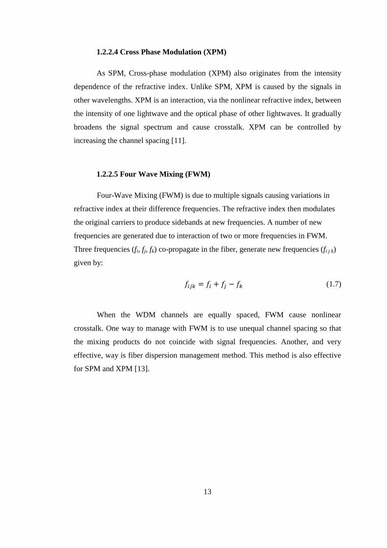
2.3.2 Return To Zero (RZ)
Recent analysis and investigations have shown that RZ turned out to be
superior compared to conventional NRZ systems. In RZ format for the logical 1 bit,
the power level returns to 0 after half of the period, whereas for the 0 bit, the power
level is 0 continuously. Binary 0 is represented by the absence of an optical pulse
during the entire bit duration.
Figure 2.5 Representation of the RZ code [19].
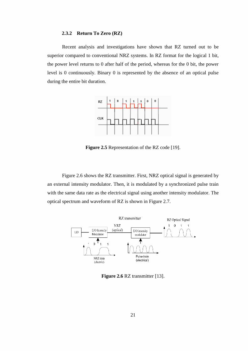
Figure 2.6 shows the RZ transmitter. First, NRZ optical signal is generated by
an external intensity modulator. Then, it is modulated by a synchronized pulse train
with the same data rate as the electrical signal using another intensity modulator. The
optical spectrum and waveform of RZ is shown in Figure 2.7.
Figure 2.6 RZ transmitter [13].
22
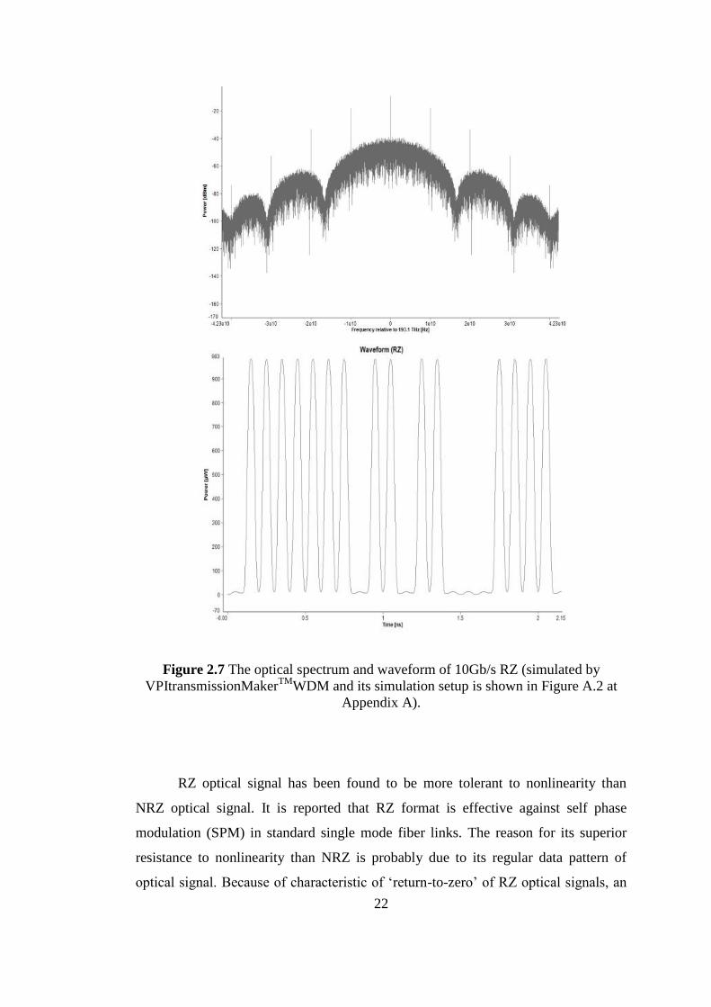
Figure 2.7 The optical spectrum and waveform of 10Gb/s RZ (simulated by
VPItransmissionMakerTM
WDM and its simulation setup is shown in Figure A.2 at
Appendix A).
RZ optical signal has been found to be more tolerant to nonlinearity than
NRZ optical signal. It is reported that RZ format is effective against self phase
modulation (SPM) in standard single mode fiber links. The reason for its superior
resistance to nonlinearity than NRZ is probably due to its regular data pattern of
optical signal. Because of characteristic of „return-to-zero‟ of RZ optical signals, an

23
isolated digital bit „1‟ and continuous digital “1”s would require the same amount of
optimal dispersion compensation for the best eye opening. So with the optimal
dispersion compensation in the system, RZ format shows better tolerance to
nonlinearity than NRZ [13].
The bandwidth required by RZ is twice larger than that of NRZ as shown in
Figure 2.8. Therefore it only requires half of NRZ power in transmission and twice
the switching time that required for NRZ. In addition RZ modulated signals is a
relatively broad optical spectrum, resulting in a reduced dispersion tolerance and a
reduced spectral efficiency.
Figure 2.8 Bandwidth of NRZ and RZ [6].
Figure 2.9 shows the optical spectrums and waveforms of a 10Gb/s RZ and
NRZ.
RZ modulation format is mostly preferred in submarine systems where more
costly transmitters and receivers are used. Terrestrial WDM transmission systems,
where cost is a primary driving factor, typically NRZ modulation format is employed
[18]. Chirped RZ (CRZ), Carrier Suppressed RZ (CSRZ) are some important
varieties of RZ format.

24
Figure 2.9 Optical Spectrum and waveform of 10Gb/s RZ and NRZ (simulated by
VPItransmissionMakerTM
WDM).

25
2.3.2.1 Chirped RZ (CRZ)
Chirped RZ (CRZ) is one of the variations of the RZ format. Figure 2.10
shows the diagram of the CRZ transmitter. The laser source is modulated with data to
create an NRZ signal, and then it enters to RZ modulator to create RZ pulses. Finally
a phase modulator is used to synchronously modulate the RZ pulse to chirp the
output with the center of the pulse having maximum chirp. The optimum phase
modulation is about 1.5 radians.
Figure 2.10 Chirped RZ transmitter [20].
In CRZ, bit-synchronous periodic chirp spectrally broadens the signal
bandwidth. Although this reduces the format‟s suitability for high spectral efficiency
WDM systems, it generally increases its robustness to fiber nonlinearity [16].
The optical spectrum and waveform of CRZ is shown in Figure 2.11.

26
Figure 2.11 The optical spectrum and waveform of 10Gb/s CRZ (simulated by
VPItransmissionMakerTM
WDM and its simulation setup is shown in Figure A.3 at
Appendix A).
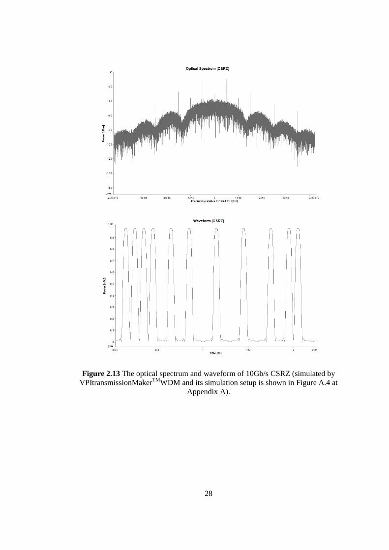
2.3.2.2 Carrier Suppressed RZ (CSRZ)
CSRZ is a special form of RZ where the carrier is suppressed. CSRZ format
reduces the nonlinear impairments in a channel and improves the spectral efficiency
in high bit rate systems. The difference between CSRZ and conventional RZ is that
the CSRZ signal has π phase shift between adjacent bits. This phase alternation, in
the optical domain, produces no DC component; thus, there is no carrier component
27
for CSRZ [17]. Phase alternating between adjacent bit slots reduces the fundamental
frequency components to half of the data rate. CSRZ has better tolerance to
chromatic dispersion due to its lower optical power, allowing for more channels
multiplexed in transmission. In addition, carrier suppression reduces the efficiency of
FWM in WDM systems [21].
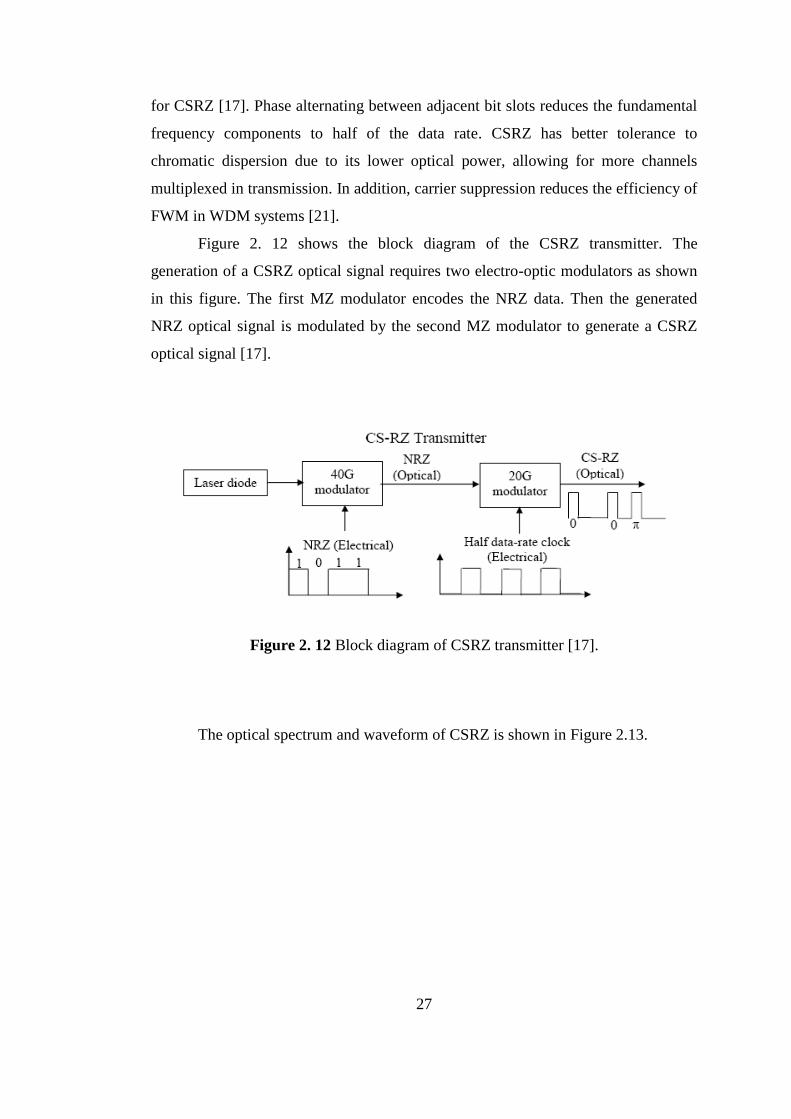
Figure 2. 12 shows the block diagram of the CSRZ transmitter. The
generation of a CSRZ optical signal requires two electro-optic modulators as shown
in this figure. The first MZ modulator encodes the NRZ data. Then the generated
NRZ optical signal is modulated by the second MZ modulator to generate a CSRZ
optical signal [17].
Figure 2. 12 Block diagram of CSRZ transmitter [17].
The optical spectrum and waveform of CSRZ is shown in Figure 2.13.
28
Figure 2.13 The optical spectrum and waveform of 10Gb/s CSRZ (simulated by
VPItransmissionMakerTM
WDM and its simulation setup is shown in Figure A.4 at
Appendix A).

29
2.3.3 Differential Phase Shift Key (DPSK)
Digital signal can be represented by instantaneous optical power levels with
optical intensity modulation. Similarly, digital signal can also be represented by the
phase of an optical carrier and this is commonly referred to as optical phase shift key
(PSK). In the early days of optical communications, the optical phase was not stable
enough for phase based modulation schemes, because of the immaturity of
semiconductor laser sources. In recent years, with the rapid improvement of single
frequency laser sources and the application of active optical phase locking, PSK
becomes feasible in practical optical systems. More specifically, differential phase
shift key (DPSK) is the most often used format [17].
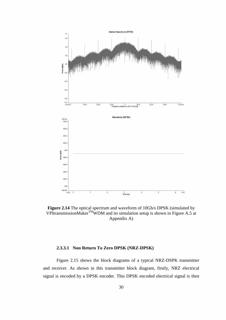
DPSK modulation is an encoding format which records changes in the binary
stream. DPSK encodes information on the binary phase change between adjacent
bits: a 1-bit is encoded onto a π phase change, whereas a 0-bit is represented by the
absence of a phase change. Like intensity modulation, DPSK can be implemented in
RZ and NRZ format. The main advantage of using DPSK with compared to intensity
modulation is a 3-dB receiver sensitivity improvement [16]. DPSK is also more
tolerant to nonlinear effects. It has better resilience to XPM and FWM, as compared
with intensity modulation formats. It has also been demonstrated that RZ-DPSK and
CSRZ-DPSK exhibit superior transmission performance than simple DPSK [14].
The optical spectrum and waveform of CSRZ is shown in Figure 2.14.
30
Figure 2.14 The optical spectrum and waveform of 10Gb/s DPSK (simulated by
VPItransmissionMakerTM
WDM and its simulation setup is shown in Figure A.5 at
Appendix A)
2.3.3.1 Non Return To Zero DPSK (NRZ-DPSK)
Figure 2.15 shows the block diagrams of a typical NRZ-DSPK transmitter
and receiver. As shown in this transmitter block diagram, firstly, NRZ electrical
signal is encoded by a DPSK encoder. This DPSK encoded electrical signal is then

31
used to drive an electro optic phase modulator to generate a DPSK optical signal. A
digital “1” is represented by a π phase change between the consecutive data bits in
the optical carrier, while there is no phase change between the consecutive data bits
in the optical carrier for a digital “0”. The important characteristic of NRZ-DPSK is
that its signal optical power is always constant [17].
Figure 2.15 Block diagrams of NRZ-DPSK transceiver and receiver [21].
As Shown in Figure 2.15, at a DPSK optical receiver, a one-bit-delay Mach-
Zehnder Interferometer (MZI) is usually used which correlates each bit with its
neighbor and makes the phase-to-intensity conversion. When the two consecutive
bits are in-phase, they are added constructively in the MZI and results in a high
signal level. Otherwise, if the there is a π phase difference between the two bits, they
cancel each other in the MZI and results in a low signal level. MZI has two balanced
output ports consist of constructive port and destructive port. A photodiode can be
used at each MZI output and then the two photocurrents are combined to double the
signal level. In this configuration, the receiver sensitivity is improved by 3dB
compared to using only a single photodiode. In a DPSK system, since signal
amplitude swings from “1” to “-1”, in the ideal case, when a balanced photo-

32
detection and matched optical filter is used, its receiver sensitivity is 3dB better than
a conventional NRZ system, where the signal swings only from “1” to “1”.
For NRZ-DPSK, the optical power is constant, however, the optical field
shifts between “1” and “-1” (or the phase shifts between “0” and “π”) and the
average optical field is zero. As a consequence, there is no carrier component in the
optical field spectrum. This differs from the spectrum of NRZ, where the carrier
component is strong [13].
The performance of NRZ-DPSK is not affected by optical power modulation
related nonlinear effect such as SPM and XPM, because of its constant optical
power. However, it is affected from chromatic dispersion. Phase modulations can be
converted into intensity modulation through group velocity dispersion (GVD), and
then SPM and XPM may contribute to waveform distortion to some extent. In a long
distance DPSK system with optical amplifiers, nonlinear phase noise is usually the
limiting factor for phase shift keying optical signals [22]. Amplified spontaneous
emission (ASE) noise generated by optical amplifiers are converted into phase noise
through the Kerr effect nonlinearity in the transmission fiber, this disturbs the signal
optical phase and causes waveform distortions [21].
2.3.3.2 Return To Zero DPSK (RZ-DPSK)
In order to improve system tolerance to nonlinear distortion and to achieve a
longer transmission distance, return-to-zero DPSK (RZ-DPSK) has been proposed.
Similar to NRZ-DPSK modulation format, the binary data is encoded as either a “0”
or a “π” phase shift between adjacent bits. In general, the width of the optical pulses
is narrower than the bit slot and therefore, the signal optical power returns to zero at
the edge of each bit slot.
Figure 2.16 shows the block diagram of a RZ-DPSK transmitter. In order to
generate the RZ-DPSK optical signal, one more intensity modulator has to be used
compare to the generation of NRZ-DPSK. First, a conventional NRZ-DPSK optical
signal is generated by an electro optic phase modulator, and then, this NRZ-DPSK
optical signal is sampled by a periodic pulse train at the clock rate through an electro
optic intensity modulator. In RZ-DPSK modulation format, the signal optical

33
intensity is no longer constant this will introduce the sensitivity to SPM. In addition,
due to the narrow pulse intensity sampling, the optical spectrum of RZ-DPSK is
wider than a conventional NRZ-DPSK. This cause more susceptibility to chromatic
dispersion. However, in long distance optical systems, periodic dispersion
compensation is often used and RZ modulation format makes it easy to find the
optimum dispersion compensation because of its regular bit patterns [21].
Figure 2.16 Block diagram of RZ-DPSK transmitter [21].
2.3.3.3 Carrier Suppressed RZ-DPSK (CSRZ-DPSK)
The significant progress made on DPSK modulation, where all formats of
ASK were tried onto the phase of the optical carrier. The transmitter consists of a
laser, followed by two dual-drive intensity modulators. This method produced phase
modulation with a near-perfect 180° phase shift. The CSRZ-DPSK pulses posses a
RZ signal shape and due to the reduced spectral width, CSRZ-DPSK modulation
shows an increased dispersion tolerance and it is more robust to nonlinear
impairments than conventional RZ format [17].
The optical spectrum and waveform of CSRZ DPSK is shown in Figure 2.17.

34
Figure 2.17 The optical spectrum and waveform of 10Gb/s CSRZ DPSK (simulated
by VPItransmissionMakerTM
WDM and its simulation setup is shown in Figure A. 6
at Appendix A)

35
CHAPTER 3
SIMULATIONS FOR MODULATION FORMATS
3.1 SIMULATION MODEL
In order to compare the transmission performances of modulation formats we
have performed a computer simulation. Firstly single channel for different modulation
formats were focused on. 40Gb/s, 100Gb/s data rate were considered. Then, channel
numbers were increased. For 40Gb/s data-rate, 25 channels were used with the channel
spacing of 160GHz (1.28nm) and total capacity was 1Tb/s. For 100Gb/s data-rate, 11
channels were used with the channel spacing of 400GHz (3.2nm) and total capacity was
1.1Tb/s. In all cases, simulations were performed in the C-band (1530nm – 1565nm).
Different fiber types and different modulation formats could affect the system
performance. In this simulations, Standard Single mode fiber (SSMF) was used.
In order to compensate the accumulated dispersion in the fiber, there are
several techniques, including Dispersion Compensating Fiber (DCF) or Fiber Bragg
Grating. In this dissertation three different schemes of dispersion compensating fiber
are used, pre-, post-, and symmetrical compensation, to compensate the fiber
dispersion. Table 3.1 lists the major physical parameters of transmission and
dispersion compensating fibers used simulations.
Table 3.1 Parameters of transmission fiber and dispersion compensating fiber at
1550nm.
Fiber Type
Dispersion
(D)
[ps/nm/km]
Dispersion
slope (S)
[ps/nm2/km]
Nonlinear
refractive
index (n2)
[10-20
m2/W]
Effective
core area
(Aeff)
[µm2]
Fiber
attenuation
(α) [dB/km]
SSMF 16x10-6
0.08x10³ 2.6x10
-20 80x10
-12 0.2x10
-3
DCF -90x10-6
0.21x10³ 2.6x10
-20 80x10
-12 0.5x10
-3

36
Pre-, post-, and symmetrical compensation configurations are shown in
Figure 3. 1 In our simulations we have used EDFA amplifiers after each fiber to
compensate for the span loss. It is the widely used amplifier type in optical
transmission systems because it provides an efficient optical amplification in the
1.55μm region.
Figure 3. 1 Configurations of the pre-, post-, and symmetrical compensation.
In pre-compensating case, DCF is precompensating the accumulated
dispersion of the transmission fiber. The gain G of the amplifier following the DCF
is balancing the fiber loss of the DCF and can be determined by:
(3.1)
where αDCF is the attenuation of the dispersion fiber, LDCF is the length of the
transmission fiber. For the gain of the amplifier succeeding the transmission fiber is a
similar equation holds. The linear dispersive compensation length of the DCF, LDCF,
should be chosen to compensate the dispersion of the transmission fiber:
(3.2)
where LTF is the length of the transmission fiber, DTF is the dispersion of the
transmission fiber, DDCF is the dispersion of the DCF.
Post-Compensating Configuration
Pre-Compensating Configuration
Symmetrical-Compensating Configuration

37
In post-compensating case, the dispersion compensating fiber (DCF) is
postcompensating the dispersion of the transmission fiber. The gain of the amplifier,
G, following the SMF compensates the fiber loss of the SMF and can be determined
by:
(3.3)
where αTF is the attenuation of the transmission fiber, LTF is the length of the
transmission fiber. For the gain of the amplifier succeeding the DCF a similar
equation holds on. The linear dispersive compensation length of the DCF should be
chosen to compensate completely the dispersion of the transmission fiber:
(3.4)
where LTF is the length of the transmission fiber, DTF is the dispersion of the
transmission fiber, DDCF is the dispersion of the DCF.
In the symmetrical compensation case, fiber placement follows the sequence
of, DCF, transmission fiber, transmission fiber, DCF [24].
3.2 PERFORMANCE ANALYSIS
The system performance was monitored by means of eye-diagram. The eye
diagram is a useful tool for the analysis of signal used in digital transmission. It
provides visual information that can be useful in the performance of transmission
systems. Many characteristics can be calculated from the eye diagram: eye width,
eye height, extinction ratio, jitter, crossing position, Q factor and bit error rate
(BER).
Figure 3.2 shows general configuration of the eye diagram and the simplified
drawing shown in Figure 3.3 [4].

38
Figure 3.2 General configuration of eye diagram.
Figure 3.3 Simplified eye diagram.
The following information can be determined from the eye diagram:
Time interval over which the received signal can be sampled without error
from intersymbol interference is defined with the width of the eye
opening.

39
The best time to sample the received waveform is when the height of the
eye opening is largest. Amplitude distortion in the data signal causes a
reduction in the height. The maximum distortion is determined from the
vertical distance between the top of the eye opening and the maximum
signal level.
The height of the eye opening at the specified sampling time shows the
noise margin or immunity to noise.
The rate at which the eye closes as the sampling time is varied determines
the sensitivity of the system to timing errors. The possibility of timing
errors increases as the slope becomes more horizontal.
Timing jitter is a phase distortion in an optical fiber system. Noise in the
receiver and pulse distortion in the optical fiber cause a jitter. Timing jitter
is thus given by
(2-3)
where ΔT is the amount of distortion at the threshold level, Tb is a bit
interval [4]. As shown in Figure 3.4, Jitter can cause a receiver to
misinterpret transmitted digital data [25].
Figure 3.4 Misinterpret transmitted digital data caused by jitter [25].

40
The rise time is defined as the time interval between the point where the
rising edge of the signal reaches 10 percent of its final amplitude and the
time it reaches 90 percent of its final amplitude. However, these points are
often obscured by noise and jitter effects so the more distinct values at the
20-percent and 80-percent threshold points are normally measured [4].
To analyze system performance BER is another method. BER is the ratio of
number of erroneous bits to the total number of bits transmitted. This error rate
depends on the signal-to-noise ratio at the receiver which is the ratio of signal power
to noise power. Q is the ratio of signal current to noise current, which is another way
to represent the signal-to-noise relationship. The larger Q is the less BER will be [4].
BER also can be evaluated by using the following formula [26].
22
1 QerfcBER
(3-5)
where erfc(x) denotes the complementary error function given by
0
22)( dyexerfc y
For telecommunications links BER of 10-9
acceptable. Typical error rates
ranges from 10-9
to 10-12
. For computer data communication links, a BER of a 10-15
is
specified. To achieve BER > 10-12
, we need to obtain Q > 7. BER of 10-9
requires
Q=6, BER of 10-15
requires Q=8 [27].
In WDM optical systems, because of the nonlinear crosstalk, the middle
channel generally has the worst performance. Channels that are far away do not
affect each other much because they pass through each other quickly due to the
dispersion. Therefore, in our simulations, we considered the middle channel of the
system.
In all simulations, VPItransmissionMakerTM
WDM software was used. The
basic mechanism behind the simulator is to solve the nonlinear Schrödinger equation
using the split-step Fourier Transformation.

41
3.3 40Gb/s WDM SYSTEM
For 40Gb/s data-rate, firstly single channel were analyzed for different
modulation formats with different compensation configuration. Then 25 channels
were used with the channel spacing of 160GHz (1.28nm) around the 193.100 THz
center frequency and total capacity was 1Tb/s.
3.3.1 Single Channel 40Gb/s WDM System
For single 40Gb/s WDM system, modulation formats of NRZ, RZ, CRZ,
CSRZ, DPSK and CSRZ-DPSK were analyzed with pre-, post- and symmetrical
compensation configurations. Total transmission distance is 12x80km=960km. for
each configuration.
3.3.1.1 NRZ Format
The simulation layouts for single channel 40Gb/s NRZ format with pre-, post
and symmetrical compensating configurations are shown in Figure A.7 at Appendix
A.
For pre- and post- compensating configurations transmission fiber length is
80km. and compensating fiber length is 14.2km evaluated using the Eq. (3.2) and Eq.
(3.4). For symmetrical compensating configuration, two transmission fibers length of
40km and two DCFs length of 7.1km were used. In all configurations, BER and eye
diagram analysis were done for 960km. fiber length.
For pre- compensating configuration, the gain of the EDFA‟s are 7.1dB and
16dB, for post- compensating configuration the gain of the EDFA‟s are 16dB and
7.1dB evaluated from Eq. (3.1) and Eq. (3.3).
The graph of BER versus Length for 40Gb/s single channel NRZ format with
all compensating configurations are shown in Figure 3.5. For all compensating case
BER is less than equal 10-9
up to 960km. As shown in this figure, BER values of pre-
and post- compensating configuration are nearly the same, post- compensating
configuration enables better performance compared to pre- compensating

42
configuration. Symmetrical compensating configuration represents the best case
among all considered configurations.
Figure 3.5 BER versus Length with all dispersion compensating configuration.
The eye diagrams of this system according to dispersion compensating
configurations are shown in Figure 3.6. The eye diagrams show the eye opening of
system for different fiber lengths. Each span is 80km. As seen from this figure eye
opening is good up to 960km.

43
Pre-compensating
configuration
Post- compensating configuration
Symmetrical- compensating
configuration
Fiber Length=80km. Fiber Length=80km. Fiber Length=80km.
Fiber Length=160km. Fiber Length=160km. Fiber Length=160km.
Fiber Length=320km. Fiber Length=320km. Fiber Length=320km.
Fiber Length=480km. Fiber Length=480km. Fiber Length=480km.
Fiber Length=720km. Fiber Length=720km Fiber Length=720km
Fiber Length=960km. Fiber Length=960km. Fiber Length=960km.
Figure 3.6 Eye diagrams of system for different fiber lengths.

44
3.3.1.2 RZ Format
The simulation layouts for single channel 40Gb/s RZ format with pre-, post
and symmetrical compensating configurations are shown in Figure A.8 at Appendix
A.
For pre- and post- compensating configurations transmission fiber length is
80km. and compensating fiber length is 14.2km evaluated using the Eq. (3.2) and Eq.
(3.4). For symmetrical compensating configuration, two transmission fibers length of
40km and two DCFs length of 7.1km were used. In all configurations, BER and eye
diagram analysis were done for 960km. fiber length.
For pre- compensating configuration, the gain of the EDFA‟s are 7.1dB and
16dB, for post- compensating configuration the gain of the EDFA‟s are 16dB and
7.1dB evaluated from Eq. (3.1) and Eq. (3.3).
The graph of BER versus Length for 40Gb/s single channel RZ format with
all compensating configurations are shown in Figure 3.7. For all compensating case
BER is less than equal 10-9
up to 960km. As shown in this figure, BER values of pre-
and post- compensating configuration are mostly the same. Symmetrical
compensating configuration represents the best case among all considered
configurations.

45
Figure 3.7 BER versus Length with all dispersion compensating configuration.
The eye diagrams of this system are shown in Figure 3.8. The eye diagrams
show the eye opening of system for different fiber lengths. Each span is 80km. As
seen from this figure eye opening is good up to 960km.

46
Pre-compensating
configuration
Post- compensating configuration
Symmetrical- compensating
configuration
Fiber Length=80km. Fiber Length=80km. Fiber Length=80km.
Fiber Length=160km. Fiber Length=160km. Fiber Length=160km.
Fiber Length=320km. Fiber Length=320km. Fiber Length=320km.
Fiber Length=480km. Fiber Length=480km. Fiber Length=480km.
Fiber Length=720km. Fiber Length=720km Fiber Length=720km
Fiber Length=960km. Fiber Length=960km. Fiber Length=960km.
Figure 3.8 Eye diagrams of system for different fiber lengths.

47
3.3.1.3 CRZ Format
The simulation layouts for single channel 40Gb/s CRZ format with pre-, post
and symmetrical compensating configurations are shown in Figure A.9 at Appendix
A.
For pre- and post- compensating configurations transmission fiber length is
80km. and compensating fiber length is 14.2km evaluated using the Eq. (3.2) and Eq.
(3.4). For symmetrical compensating configuration, two transmission fibers length of
40km and two DCFs length of 7.1km were used. In all configurations, BER and eye
diagram analysis were done for 960km. fiber length.
For pre- compensating configuration, the gain of the EDFA‟s are 7.1dB and
16dB, for post- compensating configuration the gain of the EDFA‟s are 16dB and
7.1dB evaluated from Eq. (3.1) and Eq. (3.3).
The graph of BER versus Length for 40Gb/s single channel CRZ format with
all compensating configurations are shown in Figure 3. 9. For all compensating case
BER is less than equal 10-9
up to 960km. As shown in this figure, BER values of pre-
and post- compensating configuration are mostly the same. Symmetrical
compensating configuration represents the best case among all considered
configurations.
Figure 3. 9 BER versus Length with all dispersion compensating configuration.

48
The eye diagrams of this system are shown in Figure 3.10. The eye diagrams
show the eye opening of system for different fiber lengths. Each span is 80km. As
seen from this figure eye opening is good up to 960km.
Pre-compensating
configuration
Post- compensating configuration
Symmetrical- compensating
configuration
Fiber Length=80km. Fiber Length=80km. Fiber Length=80km.
Fiber Length=160km. Fiber Length=160km. Fiber Length=160km.
Fiber Length=320km. Fiber Length=320km. Fiber Length=320km.
Fiber Length=480km. Fiber Length=480km. Fiber Length=480km.
Fiber Length=720km. Fiber Length=720km Fiber Length=720km
Fiber Length=960km. Fiber Length=960km. Fiber Length=960km.
Figure 3.10 Eye diagrams of system for different fiber lengths.
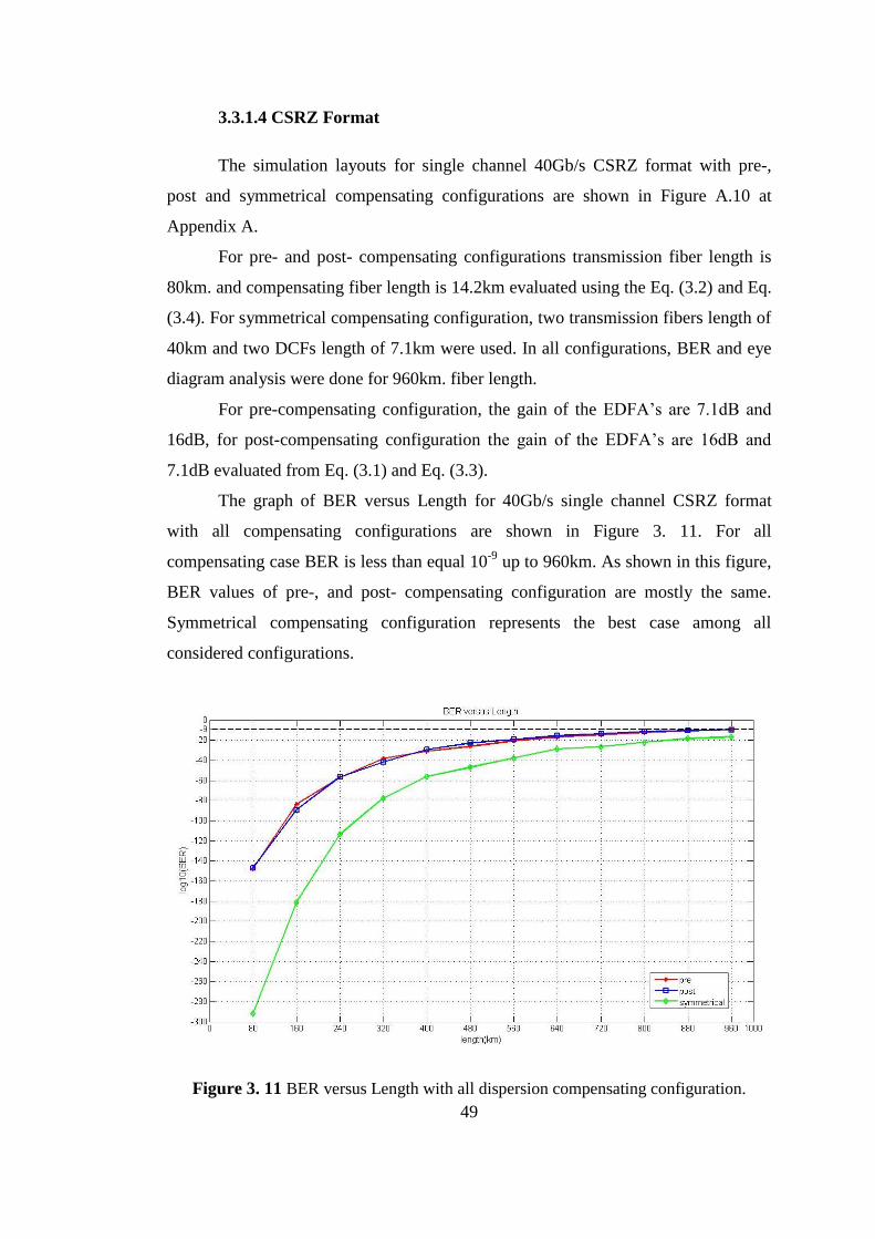
49
3.3.1.4 CSRZ Format
The simulation layouts for single channel 40Gb/s CSRZ format with pre-,
post and symmetrical compensating configurations are shown in Figure A.10 at
Appendix A.
For pre- and post- compensating configurations transmission fiber length is
80km. and compensating fiber length is 14.2km evaluated using the Eq. (3.2) and Eq.
(3.4). For symmetrical compensating configuration, two transmission fibers length of
40km and two DCFs length of 7.1km were used. In all configurations, BER and eye
diagram analysis were done for 960km. fiber length.
For pre-compensating configuration, the gain of the EDFA‟s are 7.1dB and
16dB, for post-compensating configuration the gain of the EDFA‟s are 16dB and
7.1dB evaluated from Eq. (3.1) and Eq. (3.3).
The graph of BER versus Length for 40Gb/s single channel CSRZ format
with all compensating configurations are shown in Figure 3. 11. For all
compensating case BER is less than equal 10-9
up to 960km. As shown in this figure,
BER values of pre-, and post- compensating configuration are mostly the same.
Symmetrical compensating configuration represents the best case among all
considered configurations.
Figure 3. 11 BER versus Length with all dispersion compensating configuration.

50
The eye diagrams of this system are shown in Figure 3.12. The eye diagrams
show the eye opening of system for different fiber lengths. Each span is 80km. As
seen from this figure eye opening is good up to 960km.
Pre-compensating
configuration
Post- compensating configuration
Symmetrical- compensating
configuration
Fiber Length=80km. Fiber Length=80km. Fiber Length=80km.
Fiber Length=160km. Fiber Length=160km. Fiber Length=160km.
Fiber Length=320km. Fiber Length=320km. Fiber Length=320km.
Fiber Length=480km. Fiber Length=480km. Fiber Length=480km.
Fiber Length=720km. Fiber Length=720km Fiber Length=720km
Fiber Length=960km. Fiber Length=960km. Fiber Length=960km.
Figure 3.12 Eye diagrams of system for different fiber lengths.

51
3.3.1.5 DPSK Format
The simulation layouts for single channel 40Gb/s DPSK format with pre-,
post and symmetrical compensating configurations are shown in Figure A.11 at
Appendix A.
For pre- and post- compensating configurations transmission fiber length is
80km. and compensating fiber length is 14.2km evaluated using the Eq. (3.2) and Eq.
(3.4). For symmetrical compensating configuration, two transmission fibers length of
40km and two DCFs length of 7.1km were used. In all configurations, BER and eye
diagram analysis were done for 960km. fiber length.
For pre-compensating configuration, the gain of the EDFA‟s are 7.1dB and
16dB, for post-compensating configuration the gain of the EDFA‟s are 16dB and
7.1dB evaluated from Eq. (3.1) and Eq. (3.3).
The graph of BER versus Length for 40Gb/s single channel DPSK format
with all compensating configurations are shown in Figure 3.13. For all compensating
case BER is less than equal 10-9
up to 960km. As shown in this figure, BER values of
pre-, and post- compensating configuration are mostly the same. Symmetrical
compensating configuration represents the best case among all considered
configurations.
Figure 3.13 BER versus Length with all dispersion compensating configuration.

52
The eye diagrams of this system are shown in Figure 3.14. The eye diagrams
show the eye opening of system for different fiber lengths. Each span is 80km. As
seen from this figure eye opening is good up to 960km.
Pre-compensating
configuration
Post- compensating configuration
Symmetrical- compensating
configuration
Fiber Length=80km. Fiber Length=80km. Fiber Length=80km.
Fiber Length=160km. Fiber Length=160km. Fiber Length=160km.
Fiber Length=320km. Fiber Length=320km. Fiber Length=320km.
Fiber Length=480km. Fiber Length=480km. Fiber Length=480km.
Fiber Length=720km. Fiber Length=720km Fiber Length=720km
Fiber Length=960km. Fiber Length=960km. Fiber Length=960km.
Figure 3.14 Eye diagrams of system for different fiber lengths.

53
3.3.1.6 CSRZ-DPSK Format
The simulation layouts for single channel 40Gb/s CSRZ-DPSK format with
pre-, post and symmetrical compensating configurations are shown in Figure A. 12 at
Appendix A.
For pre- and post- compensating configurations transmission fiber length is
80km. and compensating fiber length is 14.2km evaluated using the Eq. (3.2) and Eq.
(3.4). For symmetrical compensating configuration, two transmission fibers length of
40km and two DCFs length of 7.1km were used. In all configurations, BER and eye
diagram analysis were done for 960km. fiber length.
For pre-compensating configuration, the gain of the EDFA‟s are 7.1dB and
16dB, for post-compensating configuration the gain of the EDFA‟s are 16dB and
7.1dB evaluated from Eq. (3.1) and Eq. (3.3).
The graph of BER versus Length for 40Gb/s single channel CSRZ DPSK
format with all compensating configurations are shown in Figure 3.15. For all
compensating case BER is less than equal 10-9
up to 960km. As shown in this figure,
BER values of post-compensating configuration is better compared to pre-
compensating configuration. Symmetrical compensating configuration represents the
best case among all considered configurations.
Figure 3.15 BER versus Length with all dispersion compensating configuration.

54
The eye diagrams of this system are shown in Figure 3.16. The eye diagrams
show the eye opening of system for different fiber lengths. Each span is 80km. As
seen from this figure eye opening is good up to 960km.
Pre-compensating
configuration
Post- compensating configuration
Symmetrical- compensating
configuration
Fiber Length=80km. Fiber Length=80km. Fiber Length=80km.
Fiber Length=160km. Fiber Length=160km. Fiber Length=160km.
Fiber Length=320km. Fiber Length=320km. Fiber Length=320km.
Fiber Length=480km. Fiber Length=480km. Fiber Length=480km.
Fiber Length=720km. Fiber Length=720km Fiber Length=720km
Fiber Length=960km. Fiber Length=960km. Fiber Length=960km.
Figure 3.16 Eye diagrams of system for different fiber lengths.

55
Single channel 40Gb/s for all modulation formats with pre- compensating
configuration is shown in Figure 3.17. As shown in this figure the performance of
CSRZ-DPSK modulation format represents the best case among all considered
formats.
Figure 3.17 BER versus Length for single channel 40Gb/s system for all modulation
formats with pre-compensating configuration.
Figure 3.18 shows the single channel 40Gb/s for all modulation formats with
post-compensating configuration. As shown in this figure the performance of CSRZ-
DPSK modulation format represents the best case among all considered formats.

56
Figure 3.18 BER versus Length for single channel 40Gb/s system for all modulation
formats with post-compensating configuration.
Single channel 40Gb/s for all modulation formats with symmetrical
compensating configuration is shown in Figure 3.19. As shown in this figure up to
240 km. the performance of NRZ modulation format is better compared the others.
After that length CSRZ-DPSK modulation format represents the best case among all
considered formats.
Figure 3.19 BER versus Length for single channel 40Gb/s system for all modulation
formats with symmetrical compensating configuration.

57
3.3.2 25 Channels 40Gb/s WDM System
For 40Gb/s data-rate, 25 channels were used with the channel spacing of
160Ghz (1.28nm) and total capacity was 1Tb/s. For this system, modulation formats
of NRZ, RZ, CRZ, CSRZ, DPSK and CSRZ-DPSK were analyzed with pre-, post-
and symmetrical compensation configurations. Total transmission distance is
12x80km=960km. for each configuration.
In WDM optical systems, because of the nonlinear crosstalk, the middle
channel generally has the worst performance. Channels that are far away do not
affect each other much because they pass through each other quickly due to the
dispersion. Therefore, in our simulations, we considered the middle channel 13 of the
system.
3.3.2.1 25 Channels NRZ Format
The simulation layouts for 25 Channels 40Gb/s NRZ format with pre-, post
and symmetrical compensating configurations are shown in Figure A.13 at Appendix
A.
For pre- and post- compensating configurations transmission fiber length is
80km. and compensating fiber length is 14.2km evaluated using the Eq. (3.2) and Eq.
(3.4). For symmetrical compensating configuration, two transmission fibers length of
40km and two DCFs length of 7.1km were used. In all configurations, BER and eye
diagram analysis were done for 960km. fiber length.
For pre-compensating configuration, the gain of the EDFA‟s are 7.1dB and
16dB, for post-compensating configuration the gain of the EDFA‟s are 16dB and
7.1dB evaluated from Eq. (3.1) and Eq. (3.3).
The graph of BER versus Length for channel 13 based on NRZ format with
all compensating configurations are shown in Figure 3.20. For post- and pre-
compensating configurations BER is less than equal 10-9
up to 400km., for
symmetrical case it is up to 240km. As shown in this figure, BER values of post-

58
compensating configuration is better compared to symmetrical compensating
configuration. Pre- compensating configuration represents the best case among all
considered configurations.
Figure 3.20 BER versus Length with all dispersion compensating configuration.
The eye diagrams of this system are shown in Figure 3.21. The eye diagrams
show the eye opening of system for different fiber lengths. Each span is 80km. As
seen from this figure eye opening is good up to 400km.
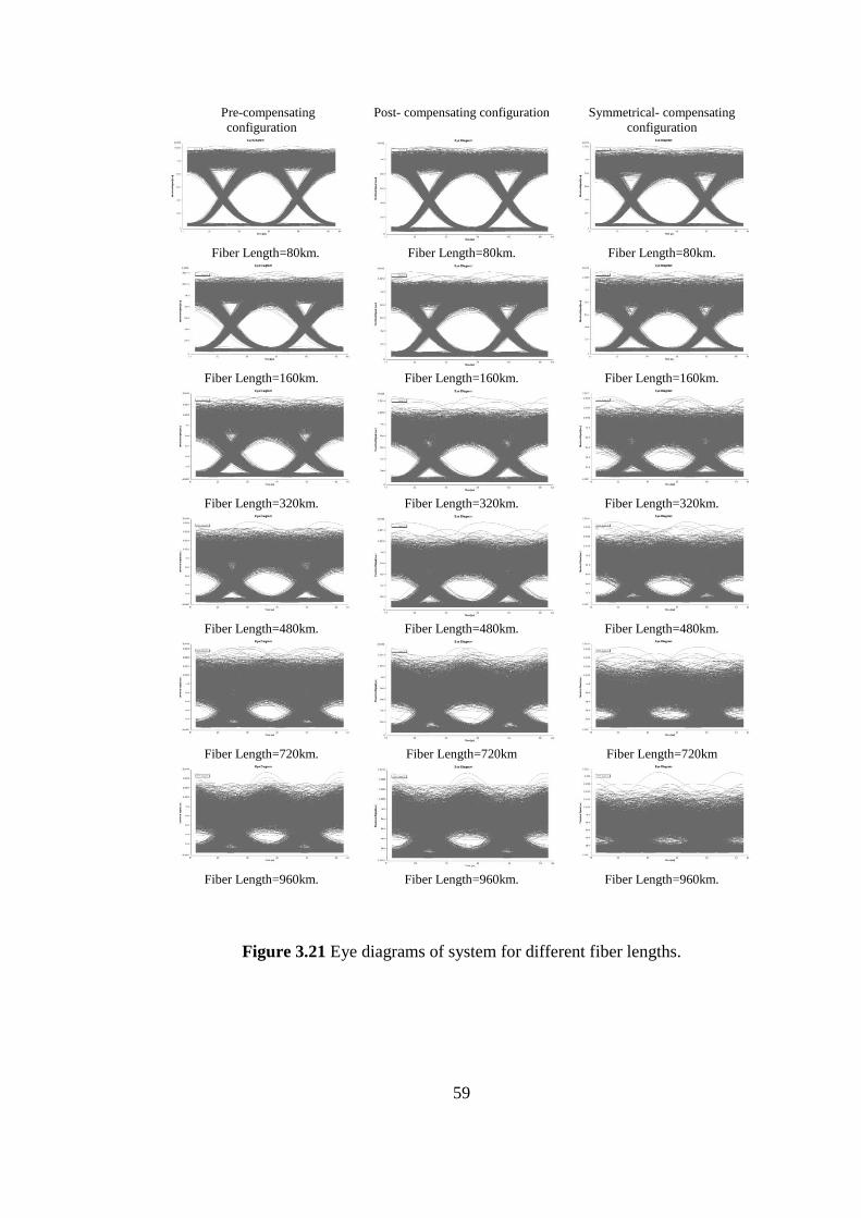
59
Pre-compensating
configuration
Post- compensating configuration
Symmetrical- compensating
configuration
Fiber Length=80km. Fiber Length=80km. Fiber Length=80km.
Fiber Length=160km. Fiber Length=160km. Fiber Length=160km.
Fiber Length=320km. Fiber Length=320km. Fiber Length=320km.
Fiber Length=480km. Fiber Length=480km. Fiber Length=480km.
Fiber Length=720km. Fiber Length=720km Fiber Length=720km
Fiber Length=960km. Fiber Length=960km. Fiber Length=960km.
Figure 3.21 Eye diagrams of system for different fiber lengths.

60
3.3.2.2 25 Channels RZ Format
The simulation layouts for 25 Channels 40Gb/s RZ format with pre-, post and
symmetrical compensating configurations are shown in Figure A.14 at Appendix A.
For pre- and post- compensating configurations transmission fiber length is
80km. and compensating fiber length is 14.2km evaluated using the Eq. (3.2) and Eq.
(3.4). For symmetrical compensating configuration, two transmission fibers length of
40km and two DCFs length of 7.1km were used. In all configurations, BER and eye
diagram analysis were done for 960km. fiber length.
For pre-compensating configuration, the gain of the EDFA‟s are 7.1dB and
16dB, for post-compensating configuration the gain of the EDFA‟s are 16dB and
7.1dB evaluated from Eq. (3.1) and Eq. (3.3).
The graph of BER versus Length for channel 13 based on RZ format with all
compensating configurations are shown in Figure 3.22. For symmetrical and pre-
compensating configuration BER is less than equal 10-9
up to 960km., and for post
case it is up to 800km. As shown in this figure, BER values of pre- compensating
configuration is better compared to post- compensating configuration. Symmetrical
compensating configuration represents the best case among all considered
configurations.
Figure 3.22 BER versus Length with all dispersion compensating configuration.

61
The eye diagrams of this system are shown in Figure 3.23. The eye diagrams
show the eye opening of system for different fiber lengths. Each span is 80km.
Pre-compensating
configuration
Post- compensating configuration
Symmetrical- compensating
configuration
Fiber Length=80km. Fiber Length=80km. Fiber Length=80km.
Fiber Length=160km. Fiber Length=160km. Fiber Length=160km.
Fiber Length=320km. Fiber Length=320km. Fiber Length=320km.
Fiber Length=480km. Fiber Length=480km. Fiber Length=480km.
Fiber Length=720km. Fiber Length=720km Fiber Length=720km
Fiber Length=960km. Fiber Length=960km. Fiber Length=960km.
Figure 3.23 Eye diagrams of system for different fiber lengths.

62
As seen from this figure eye opening is good up to 960km for symmetrical
and pre- compensating cases, for post- case is good up to 800km.
3.3.2.3 25 Channels CRZ Format
The simulation layouts for 25 Channels 40Gb/s CRZ format with pre-, post
and symmetrical compensating configurations are shown in Figure A.15 at Appendix
A.
For pre- and post- compensating configurations transmission fiber length is
80km. and compensating fiber length is 14.2km evaluated using the Eq. (3.2) and Eq.
(3.4). For symmetrical compensating configuration, two transmission fibers length of
40km and two DCFs length of 7.1km were used. In all configurations, BER and eye
diagram analysis were done for 960km. fiber length.
For pre-compensating configuration, the gain of the EDFA‟s are 7.1dB and
16dB, for post-compensating configuration the gain of the EDFA‟s are 16dB and
7.1dB evaluated from Eq. (3.1) and Eq. (3.3).
The graph of BER versus Length for channel 13 based on CRZ format with
all compensating configurations are shown in Figure 3.24. For symmetrical
compensating configuration BER is less than equal 10-9
up to 640km., for pre- and
post- cases it is up to 240km. As shown in this figure, BER values of pre- and post-
compensating configurations are mostly the same. Symmetrical compensating
configuration represents the best case among all considered configurations.

63
Figure 3.24 BER versus Length with all dispersion compensating configuration.
The eye diagrams of this system are shown in Figure 3.25. The eye diagrams
show the eye opening of system for different fiber lengths. Each span is 80km. Eye
opening is good up to 640km for symmetrical compensating case, for pre- and post-
cases are good up to 240km.

64
Pre-compensating
configuration
Post- compensating configuration
Symmetrical- compensating
configuration
Fiber Length=80km. Fiber Length=80km. Fiber Length=80km.
Fiber Length=160km. Fiber Length=160km. Fiber Length=160km.
Fiber Length=320km. Fiber Length=320km. Fiber Length=320km.
Fiber Length=480km. Fiber Length=480km. Fiber Length=480km.
Fiber Length=720km. Fiber Length=720km Fiber Length=720km
Fiber Length=960km. Fiber Length=960km. Fiber Length=960km.
Figure 3.25 Eye diagrams of system for different fiber lengths.

65
3.3.2.4 25 Channels CSRZ Format
The simulation layouts for 25 Channels 40Gb/s CSRZ format with pre-, post
and symmetrical compensating configurations are shown in Figure A.16 at Appendix
A.
For pre- and post- compensating configurations transmission fiber length is
80km. and compensating fiber length is 14.2km evaluated using the Eq. (3.2) and Eq.
(3.4). For symmetrical compensating configuration, two transmission fibers length of
40km and two DCFs length of 7.1km were used. In all configurations, BER and eye
diagram analysis were done for 960km. fiber length.
For pre-compensating configuration, the gain of the EDFA‟s are 7.1dB and
16dB, for post-compensating configuration the gain of the EDFA‟s are 16dB and
7.1dB evaluated from Eq. (3.1) and Eq. (3.3).
The graph of BER versus Length for channel 13 based on CSRZ format with
all compensating configurations are shown in Figure 3.26. For symmetrical
compensating configuration BER is less than equal 10-9
up to 960km., for post- and
pre- cases it is up to 640km. As shown in this figure, BER values of pre- and post-
compensating configurations are nearly the same. Symmetrical compensating
configuration represents the best case among all considered configurations.
Figure 3.26 BER versus Length with all dispersion compensating configuration.

66
Pre-compensating configuration Post- compensating configuration
Symmetrical- compensating
configuration
Fiber Length=80km. Fiber Length=80km. Fiber Length=80km.
Fiber Length=160km. Fiber Length=160km. Fiber Length=160km.
Fiber Length=320km. Fiber Length=320km. Fiber Length=320km.
Fiber Length=480km. Fiber Length=480km. Fiber Length=480km.
Fiber Length=720km. Fiber Length=720km Fiber Length=720km
Fiber Length=960km. Fiber Length=960km. Fiber Length=960km.
Figure 3. 27 Eye diagrams of system for different fiber lengths.
The eye diagrams of this system are shown in Figure 3. 27. The eye diagrams
show the eye opening of system for different fiber lengths. Each span is 80km. Eye
opening is good up to 960km for symmetrical compensating case, for pre- and post-
cases are good up to 640km.

67
3.3.2.5 25 Channels DPSK Format
The simulation layouts for 25 Channels 40Gb/s DPSK format with pre-, post
and symmetrical compensating configurations are shown in Figure A. 17 at
Appendix A.
For pre- and post- compensating configurations transmission fiber length is
80km. and compensating fiber length is 14.2km evaluated using the Eq. (3.2) and Eq.
(3.4). For symmetrical compensating configuration, two transmission fibers length of
40km and two DCFs length of 7.1km were used. In all configurations, BER and eye
diagram analysis were done for 960km. fiber length.
For pre-compensating configuration, the gain of the EDFA‟s are 7.1dB and
16dB, for post-compensating configuration the gain of the EDFA‟s are 16dB and
7.1dB evaluated from Eq. (3.1)and Eq. (3.3).
The graph of BER versus Length for channel 13 based on DPSK format with
all compensating configurations are shown in Figure 3.28. For post- and pre-
compensating configurations BER is less than equal 10-9
up to 720km., for
symmetrical- case it is up to 480km. As shown in this figure, BER values of pre-
compensating configuration is better compared to symmetrical compensating
configuration. Post- compensating configuration represents the best case among all
considered configurations.

68
Figure 3.28 BER versus Length with all dispersion compensating configuration.
The eye diagrams of this system are shown in Figure 3.29. The eye diagrams
show the eye opening of system for different fiber lengths. Each span is 80km. Eye
opening is good up to 720km for pre- and post- compensating cases, 480km. for
symmetrical case.

69
Pre-compensating configuration Post- compensating configuration
Symmetrical- compensating
configuration
Fiber Length=80km. Fiber Length=80km. Fiber Length=80km.
Fiber Length=160km. Fiber Length=160km. Fiber Length=160km.
Fiber Length=320km. Fiber Length=320km. Fiber Length=320km.
Fiber Length=480km. Fiber Length=480km. Fiber Length=480km.
Fiber Length=720km. Fiber Length=720km Fiber Length=720km
Fiber Length=960km. Fiber Length=960km. Fiber Length=960km.
Figure 3.29 Eye diagrams of system for different fiber lengths.

70
3.3.2.6 25 Channels CSRZ DPSK Format
The simulation layouts for 25 Channels 40Gb/s CSRZ DPSK format with
pre-, post and symmetrical compensating configurations are shown in Figure A.16 at
Appendix A.
For pre- and post- compensating configurations transmission fiber length is
80km. and compensating fiber length is 14.2km evaluated using the Eq. (3.2) and Eq.
(3.4). For symmetrical compensating configuration, two transmission fibers length of
40km and two DCFs length of 7.1km were used. In all configurations, BER and eye
diagram analysis were done for 960km. fiber length.
For pre-compensating configuration, the gain of the EDFA‟s are 7.1dB and
16dB, for post-compensating configuration the gain of the EDFA‟s are 16dB and
7.1dB evaluated from Eq. (3.1)and Eq. (3.3).
The graph of BER versus Length for channel 13 based on CSRZ DPSKformat
with all compensating configurations are shown in Figure 3.30. For all compensating
configurations BER is less than equal 10-9
up to 960km. As shown in this figure,
BER values of post- compensating configuration is better compared to pre-
compensating configuration. Symmetrical compensating configuration represents the
best case among all considered configurations.
Figure 3.30 BER versus Length with all dispersion compensating configuration.

71
Pre-compensating configuration Post- compensating configuration
Symmetrical- compensating
configuration
Fiber Length=80km. Fiber Length=80km. Fiber Length=80km.
Fiber Length=160km. Fiber Length=160km. Fiber Length=160km.
Fiber Length=320km. Fiber Length=320km. Fiber Length=320km.
Fiber Length=480km. Fiber Length=480km. Fiber Length=480km.
Fiber Length=720km. Fiber Length=720km Fiber Length=720km
Fiber Length=960km. Fiber Length=960km. Fiber Length=960km.
Figure 3.31 Eye diagrams of system for different fiber lengths.

72
The eye diagrams of this system are shown in Figure 3.31. The eye diagrams
show the eye opening of system for different fiber lengths. Each span is 80km. Eye
opening is good up to 240km for symmetrical compensating case, for pre- and post-
cases are good up to 160km.
25 channels 40Gb/s for all modulation formats with pre- compensating
configuration is shown in Figure 3.32. As shown in this figure the performance of
CSRZ-DPSK modulation format represents the best case among all considered
formats. RZ is also good. CRZ is the worst case.
Figure 3.32 BER versus Length for 25 channels 40Gb/s system for all modulation
formats with pre-compensating configuration.
Figure 3.33 shows the 25 channels 40Gb/s for all modulation formats with
post-compensating configuration. As shown in this figure the performance of CSRZ-
DPSK modulation format represents the best case among all considered formats. RZ
and DPSK are good up to 800km. CRZ is the worst case.

73
Figure 3.33 BER versus Length for 25 channels 40Gb/s system for all modulation
formats with post-compensating configuration.
25 channels 40Gb/s for all modulation formats with symmetrical
compensating configuration is shown in Figure 3.34. As shown in this figure CSRZ-
DPSK modulation format represents the best case among all considered formats. RZ
and CSRZ are good up to 960km. CRZ is the worst case.

74
Figure 3.34 BER versus Length for 25 channels 40Gb/s system for all modulation
formats with symmetrical compensating configuration.
3.4 100 Gb/s WDM SYSTEM
For 100Gb/s data-rate, firstly single channel were analyzed for different
modulation formats with different compensation configuration. Then 11 channels
were used with the channel spacing of 400GHz (3.2nm) around the 193.100 THz
center frequency and total capacity was 1.1Tb/s.
3.3.1 Single Channel 100Gb/s WDM System
For single 100Gb/s WDM system, modulation formats of NRZ, RZ, CRZ,
CSRZ, DPSK and CSRZ-DPSK were analyzed with pre-, post- and symmetrical
compensation configurations.
The effect of nonlinearities and dispersion in fiber is increased when the data
rate is increased. Therefore, in 100Gb/s data rate 40km fiber length span was used
and total transmission distance is 6x40km=240km.

75
3.3.1.1 NRZ Format
The simulation layouts for single channel 100Gb/s NRZ format with pre-,
post and symmetrical compensating configurations are same as 40Gb/s NRZ format
except the data rate, transmission fiber length, dispersion compensating fiber length
and EDFA gain.
For pre- and post- compensating configurations transmission fiber length is
40km. and compensating fiber length is 7.1 km evaluated using the Eq. (3.2) and Eq.
(3.4). For symmetrical compensating configuration, two transmission fibers each
length of 20km and two DCFs each length of 3.55km were used. In all
configurations, BER and eye diagram analysis were done for 240km. fiber length.
For pre-compensating configuration, the gain of the EDFA‟s are 3.55dB and
8dB, for post-compensating configuration the gain of the EDFA‟s are 8dB and
3.55dB evaluated from Eq. (3.1) and Eq. (3.3).
The graph of BER versus Length for 100Gb/s single channel NRZ format
with all compensating configurations are shown in Figure 3.35. For pre- and post-
compensating configurations BER is less than equal 10-9
up to 240km. for all
compensating configurations. As shown in this figure, BER values of post-
compensating configuration are better than pre- compensating configuration.
Symmetrical compensating configuration represents the best case among all
considered configurations.
Figure 3.35 BER versus Length with all dispersion compensating configuration.

76
Pre-compensating
configuration
Post- compensating configuration
Symmetrical- compensating
configuration
Fiber Length=40km. Fiber Length=40km. Fiber Length=40km.
Fiber Length=80km. Fiber Length=80km. Fiber Length=80km.
Fiber Length=160km. Fiber Length=160km. Fiber Length=160km.
Fiber Length=160km. Fiber Length=160km. Fiber Length=160km.
Fiber Length=200km. Fiber Length=200km. Fiber Length=200km.
Fiber Length=240km. Fiber Length=240km. Fiber Length=240km.
Figure 3.36 Eye diagrams of system for different fiber lengths; (a) Pre-compensating
configuration, (b) Post-compensating configuration, (c) Symmetrical compensating
configuration.

77
The eye diagrams of this system are shown in Figure 3.36. The eye diagrams
show the eye opening of system for different fiber lengths. Each span is 40km. As
seen from this figure eye opening is good up to 240km. for all compensating
configuration.
3.3.1.2 RZ Format
The simulation layouts for single channel 100Gb/s RZ format with pre-, post
and symmetrical compensating configurations are same as 40Gb/s RZ format except
the data rate, transmission fiber length, dispersion compensating fiber length and
EDFA gain.
For pre- and post- compensating configurations transmission fiber length is
40km. and compensating fiber length is 7.1 km evaluated using the Eq. (3.2) and Eq.
(3.4). For symmetrical compensating configuration, two transmission fibers each
length of 20km and two DCFs each length of 3.55km were used. In all
configurations, BER and eye diagram analysis were done for 240km. fiber length.
For pre-compensating configuration, the gain of the EDFA‟s are 3.55dB and
8dB, for post-compensating configuration the gain of the EDFA‟s are 8dB and
3.55dB evaluated from Eq. (3.1) and Eq. (3.3).
The graph of BER versus Length for 100Gb/s single channel RZ format with
all compensating configurations are shown in Figure 3.37. For all compensating
configurations BER is less than equal 10-9
up to 200km. As shown in this figure,
BER values of post- and pre- compensating configurations are mostly the same.
Symmetrical compensating configuration represents the best case among all
considered configurations.

78
Figure 3.37 BER versus Length with all dispersion compensating configuration.
The eye diagrams of this system are shown in Figure 3.38. The eye diagrams
show the eye opening of system for different fiber lengths. Each span is 40km. As
seen from this figure eye opening is good up to 200km. for all compensating cases.

79
Pre-compensating
configuration
Post- compensating configuration
Symmetrical- compensating
configuration
Fiber Length=40km. Fiber Length=40km. Fiber Length=40km.
Fiber Length=80km. Fiber Length=80km. Fiber Length=80km.
Fiber Length=120km. Fiber Length=120km. Fiber Length=120km.
Fiber Length=160km. Fiber Length=160km. Fiber Length=160km.
Fiber Length=200km. Fiber Length=200km. Fiber Length=200km.
Fiber Length=240km. Fiber Length=240km. Fiber Length=240km.
Figure 3.38 Eye diagrams of system for different fiber lengths; (a) Pre-compensating
configuration, (b) Post-compensating configuration, (c) Symmetrical compensating
configuration.

80
3.3.1.3 CRZ Format
The simulation layouts for single channel 100Gb/s CRZ format with pre-,
post and symmetrical compensating configurations are same as 40Gb/s CRZ format
except the data rate, transmission fiber length, dispersion compensating fiber length
and EDFA gain.
For pre- and post- compensating configurations transmission fiber length is
40km. and compensating fiber length is 7.1 km evaluated using the Eq. (3.2) and Eq.
(3.4). For symmetrical compensating configuration, two transmission fibers each
length of 20km and two DCFs each length of 3.55km were used. In all
configurations, BER and eye diagram analysis were done for 240km. fiber length.
For pre-compensating configuration, the gain of the EDFA‟s are 3.55dB and
8dB, for post-compensating configuration the gain of the EDFA‟s are 8dB and
3.55dB evaluated from Eq. (3.1) and Eq. (3.3).
The graph of BER versus Length for 100Gb/s single channel CRZ format
with all compensating configurations are shown in Figure 3.39. For all compensating
configurations BER is less than equal 10-9
up to 80km. As shown in this figure, BER
values of all compensating configurations are mostly the same. Symmetrical
compensating configuration represents the best case among all considered
configurations.

81
Figure 3.39 BER versus Length with all dispersion compensating configuration.
The eye diagrams of this system are shown in Figure 3.40. The eye diagrams
show the eye opening of system for different fiber lengths. Each span is 40km. As
seen from this figure eye opening is good up to 80km.

82
Pre-compensating
configuration
Post- compensating configuration
Symmetrical- compensating
configuration
Fiber Length=40km. Fiber Length=40km. Fiber Length=40km.
Fiber Length=80km. Fiber Length=80km. Fiber Length=80km.
Fiber Length=120km. Fiber Length=120km. Fiber Length=120km.
Fiber Length=160km. Fiber Length=160km. Fiber Length=160km.
Fiber Length=200km. Fiber Length=200km. Fiber Length=200km..
Fiber Length=240km. Fiber Length=240km. Fiber Length=240km.
Figure 3.40 Eye diagrams of system for different fiber lengths; (a) Pre-compensating
configuration, (b) Post-compensating configuration, (c) Symmetrical compensating
configuration.
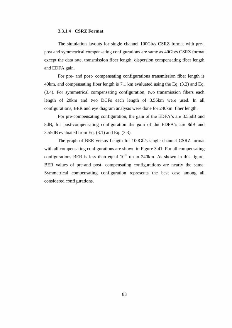
83
3.3.1.4 CSRZ Format
The simulation layouts for single channel 100Gb/s CSRZ format with pre-,
post and symmetrical compensating configurations are same as 40Gb/s CSRZ format
except the data rate, transmission fiber length, dispersion compensating fiber length
and EDFA gain.
For pre- and post- compensating configurations transmission fiber length is
40km. and compensating fiber length is 7.1 km evaluated using the Eq. (3.2) and Eq.
(3.4). For symmetrical compensating configuration, two transmission fibers each
length of 20km and two DCFs each length of 3.55km were used. In all
configurations, BER and eye diagram analysis were done for 240km. fiber length.
For pre-compensating configuration, the gain of the EDFA‟s are 3.55dB and
8dB, for post-compensating configuration the gain of the EDFA‟s are 8dB and
3.55dB evaluated from Eq. (3.1) and Eq. (3.3).
The graph of BER versus Length for 100Gb/s single channel CSRZ format
with all compensating configurations are shown in Figure 3.41. For all compensating
configurations BER is less than equal 10-9
up to 240km. As shown in this figure,
BER values of pre-and post- compensating configurations are nearly the same.
Symmetrical compensating configuration represents the best case among all
considered configurations.

84
Figure 3.41 BER versus Length with all dispersion compensating configuration.
The eye diagrams of this system are shown in Figure 3.42. The eye diagrams
show the eye opening of system for different fiber lengths. Each span is 40km. As
seen from this figure eye opening is good up to 240km.

85
Pre-compensating
configuration
Post- compensating configuration
Symmetrical- compensating
configuration
Fiber Length=40km. Fiber Length=40km. Fiber Length=40km.
Fiber Length=80km. Fiber Length=80km. Fiber Length=80km.
Fiber Length=120km. Fiber Length=120km. Fiber Length=120km.
Fiber Length=160km. Fiber Length=160km. Fiber Length=160km.
Fiber Length=200km. Fiber Length=200km. Fiber Length=200km.
Fiber Length=240km. Fiber Length=240km. Fiber Length=240km.
Figure 3.42 Eye diagrams of system for different fiber lengths; (a) Pre-compensating
configuration, (b) Post-compensating configuration, (c) Symmetrical compensating
configuration.

86
3.3.1.5 DPSK Format
The simulation layouts for single channel 100Gb/s DPSK format with pre-,
post and symmetrical compensating configurations are same as 40Gb/s DPSK format
except the data rate, transmission fiber length, dispersion compensating fiber length
and EDFA gain.
For pre- and post- compensating configurations transmission fiber length is
40km. and compensating fiber length is 7.1 km evaluated using the Eq. (3.2) and Eq.
(3.4). For symmetrical compensating configuration, two transmission fibers each
length of 20km and two DCFs each length of 3.55km were used. In all
configurations, BER and eye diagram analysis were done for 240km. fiber length.
For pre-compensating configuration, the gain of the EDFA‟s are 3.55dB and
8dB, for post-compensating configuration the gain of the EDFA‟s are 8dB and
3.55dB evaluated from Eq. (3.1) and Eq. (3.3).
The graph of BER versus Length for 100Gb/s single channel DPSK format
with all compensating configurations are shown in Figure 3.43. For all compensating
configurations BER is less than equal 10-9
up to 240km. As shown in this figure,
BER values of all compensating configurations are mostly the same. Symmetrical
compensating configuration represents the best case among all considered
configurations.
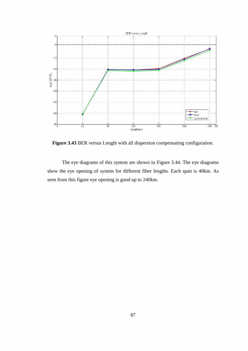
87
Figure 3.43 BER versus Length with all dispersion compensating configuration.
The eye diagrams of this system are shown in Figure 3.44. The eye diagrams
show the eye opening of system for different fiber lengths. Each span is 40km. As
seen from this figure eye opening is good up to 240km.

88
Pre-compensating
configuration
Post- compensating configuration
Symmetrical- compensating
configuration
Fiber Length=40km. Fiber Length=40km. Fiber Length=40km.
Fiber Length=80km. Fiber Length=80km. Fiber Length=80km.
Fiber Length=120km. Fiber Length=120km. Fiber Length=120km.
Fiber Length=160km. Fiber Length=160km. Fiber Length=160km.
Fiber Length=200km. Fiber Length=200km. Fiber Length=200km.
Fiber Length=240km. Fiber Length=240km. Fiber Length=240km.
Figure 3.44 Eye diagrams of system for different fiber lengths; (a) Pre-compensating
configuration, (b) Post-compensating configuration, (c) Symmetrical compensating
configuration.

89
3.3.1.6 CSRZ DPSK Format
The simulation layouts for single channel 100Gb/s CSRZ DPSK format with
pre-, post and symmetrical compensating configurations are same as 40Gb/s CSRZ
DPSK format except the data rate, transmission fiber length, dispersion
compensating fiber length and EDFA gain.
For pre- and post- compensating configurations transmission fiber length is
40km. and compensating fiber length is 7.1 km evaluated using the Eq. (3.2) and Eq.
(3.4). For symmetrical compensating configuration, two transmission fibers each
length of 20km and two DCFs each length of 3.55km were used. In all
configurations, BER and eye diagram analysis were done for 240km. fiber length.
For pre-compensating configuration, the gain of the EDFA‟s are 3.55dB and
8dB, for post-compensating configuration the gain of the EDFA‟s are 8dB and
3.55dB evaluated from Eq. (3.1) and Eq. (3.3).
The graph of BER versus Length for 100Gb/s single channel CSRZ DPSK
format with all compensating configurations are shown in Figure 3.45. For all
compensating configurations BER is less than equal 10-9
up to 240km. As shown in
this figure, BER values of post- and symmetrical compensating configurations are
nearly the same and are better compared to pre- compensating configuration.
Symmetrical compensating configuration represents the best case among all
considered configurations.
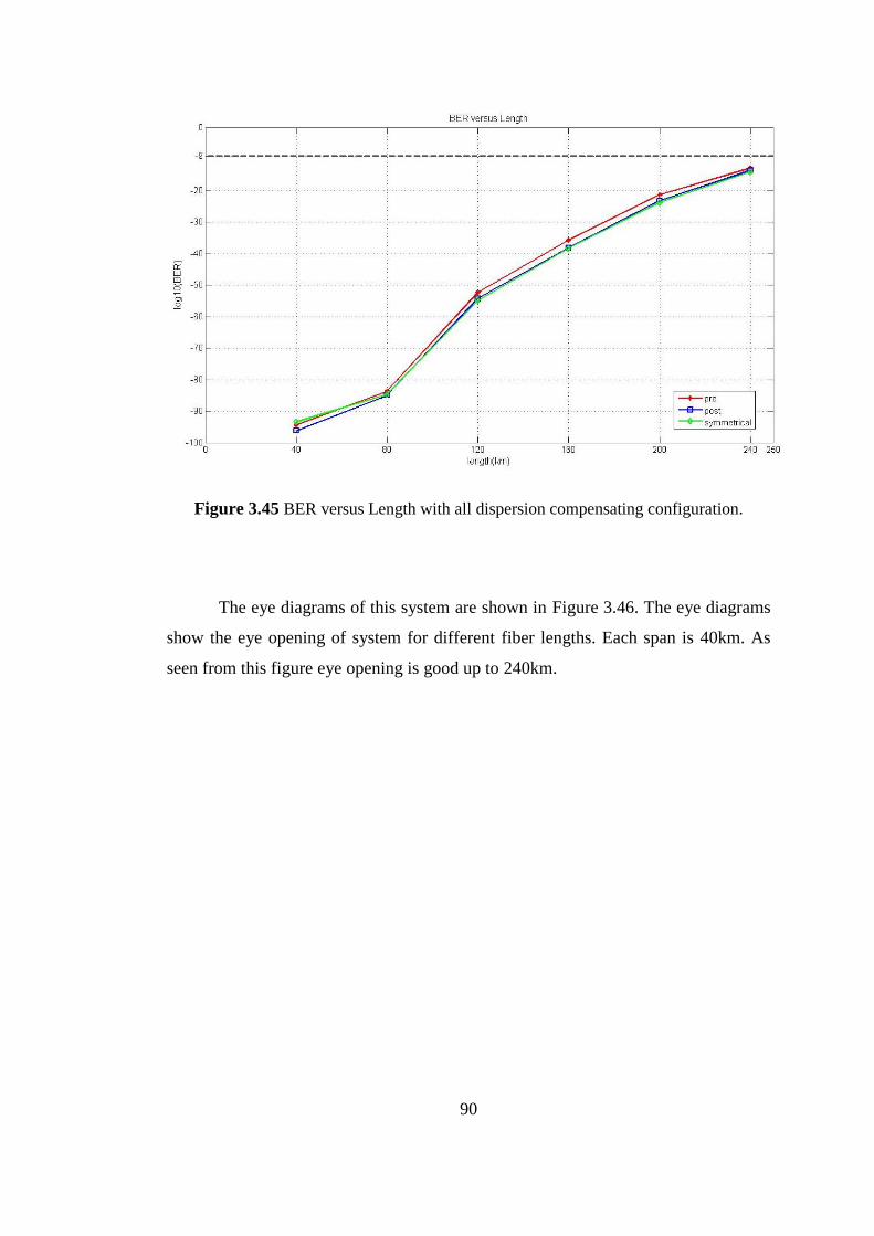
90
Figure 3.45 BER versus Length with all dispersion compensating configuration.
The eye diagrams of this system are shown in Figure 3.46. The eye diagrams
show the eye opening of system for different fiber lengths. Each span is 40km. As
seen from this figure eye opening is good up to 240km.
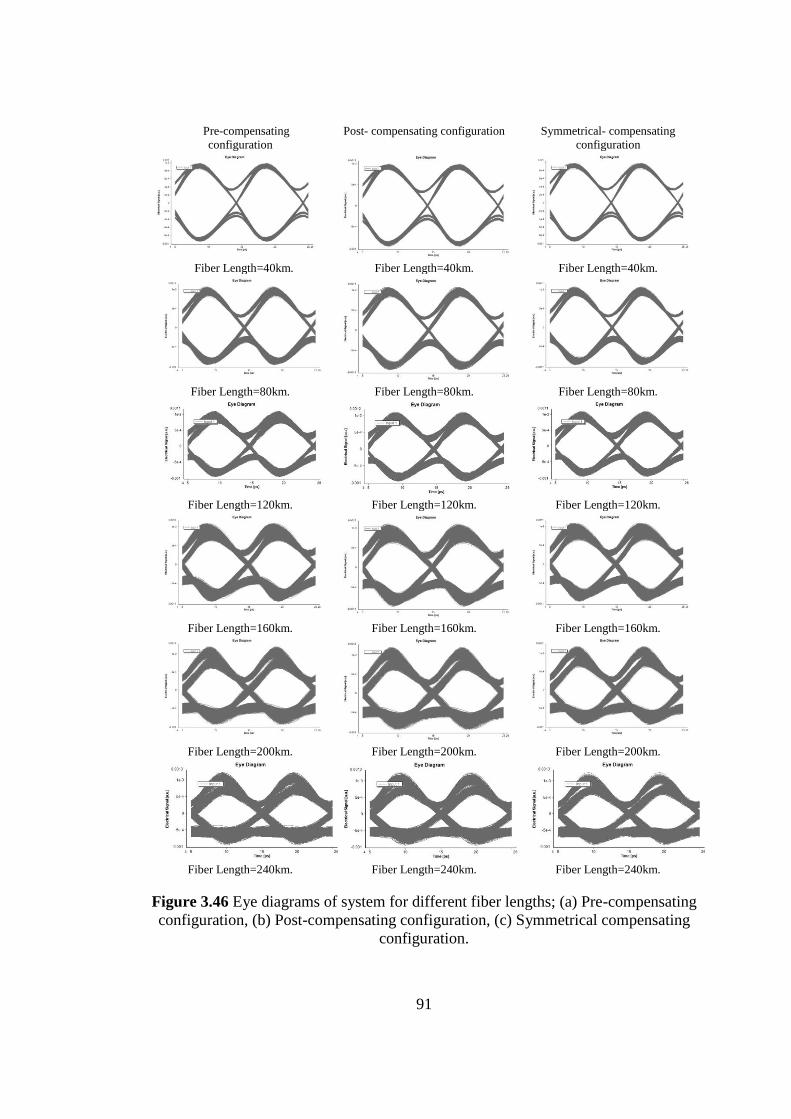
91
Pre-compensating
configuration
Post- compensating configuration
Symmetrical- compensating
configuration
Fiber Length=40km. Fiber Length=40km. Fiber Length=40km.
Fiber Length=80km. Fiber Length=80km. Fiber Length=80km.
Fiber Length=120km. Fiber Length=120km. Fiber Length=120km.
Fiber Length=160km. Fiber Length=160km. Fiber Length=160km.
Fiber Length=200km. Fiber Length=200km. Fiber Length=200km.
Fiber Length=240km. Fiber Length=240km. Fiber Length=240km.
Figure 3.46 Eye diagrams of system for different fiber lengths; (a) Pre-compensating
configuration, (b) Post-compensating configuration, (c) Symmetrical compensating
configuration.

92
Single channel 100Gb/s for all modulation formats with pre- compensating
configuration is shown in Figure 3.47. As shown in this figure the performance of
RZ is better compared to others up to 120km. CSRZ-DPSK modulation format
represents the best case among all considered formats up to 240km.
Figure 3.47 BER versus Length for single channel 100Gb/s system for all modulation
formats with pre-compensating configuration.
Figure 3.48 shows the single channel 100Gb/s for all modulation formats with
post-compensating configuration. As shown in this figure the performance of RZ is
better compared to others up to 120km. CSRZ-DPSK modulation format represents
the best case among all considered formats up to 240km.

93
Figure 3.48 BER versus Length for single channel 100Gb/s system for all modulation
formats with post-compensating configuration.
Single channel 100Gb/s for all modulation formats with symmetrical
compensating configuration is shown in Figure 3.49. As shown in this figure the
performance of RZ is better compared to others up to 120km. CSRZ-DPSK
modulation format represents the best case among all considered formats up to
240km.

94
Figure 3.49 BER versus Length for single channel 100Gb/s system for all modulation
formats with symmetrical compensating configuration.
3.3.2 11 Channels 100Gb/s WDM System
For 100Gb/s data-rate, 11 channels were used with the channel spacing of
400Ghz (3.2nm) and total capacity was 1.1Tb/s. For this system, modulation formats
of NRZ, RZ, CRZ, CSRZ, DPSK and CSRZ-DPSK were analyzed with pre-, post-
and symmetrical compensation configurations. Total transmission distance is
6x40km=240km. for each configuration.
In WDM optical systems, because of the nonlinear crosstalk, the middle
channel generally has the worst performance. Channels that are far away do not
affect each other much because they pass through each other quickly due to the
dispersion. Therefore, in our simulations, we considered the middle channel 6 of the
system.

95
3.3.2.1 NRZ Format
The simulation layouts for 11 channel 100Gb/s NRZ format with pre-, post
and symmetrical compensating configurations are same as 40Gb/s NRZ format
except the data rate, transmission fiber length, dispersion compensating fiber length
and EDFA gain.
For pre- and post- compensating configurations transmission fiber length is
40km. and compensating fiber length is 7.1 km evaluated using the Eq. (3.2) and Eq.
(3.4). For symmetrical compensating configuration, two transmission fibers each
length of 20km and two DCFs each length of 3.55km were used. In all
configurations, BER and eye diagram analysis were done for 240km. fiber length.
For pre-compensating configuration, the gain of the EDFA‟s are 3.55dB and
8dB, for post-compensating configuration the gain of the EDFA‟s are 8dB and
3.55dB evaluated from Eq. (3.1) and Eq. (3.3).
The graph of BER versus Length for 100Gb/s 11 channels NRZ format with
all compensating configurations are shown in Figure 3.50. For all compensating
configurations BER is less than equal 10-9
up to 240km. As shown in this figure,
BER values of post- compensating configuration is better compared to symmetrical
compensating configuration. Pre- compensating configuration represents the best
case among all considered configurations.
Figure 3.50 BER versus Length with all dispersion compensating configuration.

96
The eye diagrams of this system are shown in Figure 3.51. The eye diagrams
show the eye opening of system for different fiber lengths. Each span is 40km. As
seen from this figure eye opening is good up to 240km.
Pre-compensating
configuration
Post- compensating configuration
Symmetrical- compensating
configuration
Fiber Length=40km. Fiber Length=40km. Fiber Length=40km.
Fiber Length=80km. Fiber Length=80km. Fiber Length=80km.
Fiber Length=120km. Fiber Length=120km. Fiber Length=120km.
Fiber Length=160km. Fiber Length=160km. Fiber Length=160km.
Fiber Length=200km. Fiber Length=200km. Fiber Length=200km.
Fiber Length=240km. Fiber Length=240km. Fiber Length=240km.
Figure 3.51 Eye diagrams of system for different fiber lengths; (a) Pre-compensating
configuration, (b) Post-compensating configuration, (c) Symmetrical compensating
configuration.

97
3.3.2.2 RZ Format
The simulation layouts for 11 channel 100Gb/s RZ format with pre-, post and
symmetrical compensating configurations are same as 40Gb/s RZ format except the
data rate, transmission fiber length, dispersion compensating fiber length and EDFA
gain.
For pre- and post- compensating configurations transmission fiber length is
40km. and compensating fiber length is 7.1 km evaluated using the Eq. (3.2) and Eq.
(3.4). For symmetrical compensating configuration, two transmission fibers each
length of 20km and two DCFs each length of 3.55km were used. In all
configurations, BER and eye diagram analysis were done for 240km. fiber length.
For pre-compensating configuration, the gain of the EDFA‟s are 3.55dB and
8dB, for post-compensating configuration the gain of the EDFA‟s are 8dB and
3.55dB evaluated from Eq. (3.1) and Eq. (3.3).
The graph of BER versus Length for 100Gb/s 11 channels RZ format with all
compensating configurations are shown in Figure 3.52. For all compensating
configurations BER is less than equal 10-9
up to 200km. As shown in this figure, pre
case is better compared to post case. Symmetrical compensating configuration
represents the best case among all considered configurations.

98
Figure 3.52 BER versus Length with all dispersion compensating configuration.
The eye diagrams of this system are shown in Figure 3.53. The eye diagrams
show the eye opening of system for different fiber lengths. Each span is 40km. As
seen from this figure eye opening is good up to 200km.

99
Pre-compensating
configuration
Post- compensating configuration
Symmetrical- compensating
configuration
Fiber Length=40km. Fiber Length=40km. Fiber Length=40km.
Fiber Length=80km. Fiber Length=80km. Fiber Length=80km.
Fiber Length=120km. Fiber Length=120km. Fiber Length=120km.
Fiber Length=160km. Fiber Length=160km. Fiber Length=160km.
Fiber Length=200km. Fiber Length=200km. Fiber Length=200km.
Fiber Length=240km. Fiber Length=240km. Fiber Length=240km.
Figure 3.53 Eye diagrams of system for different fiber lengths; (a) Pre-compensating
configuration, (b) Post-compensating configuration, (c) Symmetrical compensating
configuration.

100
3.3.2.3 CRZ Format
The simulation layouts for 11 channel 100Gb/s CRZ format with pre-, post
and symmetrical compensating configurations are same as 40Gb/s CRZ format
except the data rate, transmission fiber length, dispersion compensating fiber length
and EDFA gain.
For pre- and post- compensating configurations transmission fiber length is
40km. and compensating fiber length is 7.1 km evaluated using the Eq. (3.2) and Eq.
(3.4). For symmetrical compensating configuration, two transmission fibers each
length of 20km and two DCFs each length of 3.55km were used. In all
configurations, BER and eye diagram analysis were done for 240km. fiber length.
For pre-compensating configuration, the gain of the EDFA‟s are 3.55dB and
8dB, for post-compensating configuration the gain of the EDFA‟s are 8dB and
3.55dB evaluated from Eq. (3.1) and Eq. (3.3).
The graph of BER versus Length for 100Gb/s 11 channels CRZ format with
all compensating configurations are shown in Figure 3.54. For all compensating
configurations BER is less than equal 10-9
up to 120km. As shown in this figure,
BER values of post- and pre- compensating configurations are nearly the same.
Symmetrical compensating configuration represents the best case among all
considered configurations.

101
Figure 3.54 BER versus Length with all dispersion compensating configuration.
The eye diagrams of this system are shown in Figure 3.55. The eye diagrams
show the eye opening of system for different fiber lengths. Each span is 40km. As
seen from this figure eye opening is good up to 120km.

102
Pre-compensating
configuration
Post- compensating configuration
Symmetrical- compensating
configuration
Fiber Length=40km. Fiber Length=40km. Fiber Length=40km.
Fiber Length=80km. Fiber Length=80km. Fiber Length=80km.
Fiber Length=120km. Fiber Length=120km. Fiber Length=120km.
Fiber Length=160km. Fiber Length=160km. Fiber Length=160km.
Fiber Length=200km. Fiber Length=200km. Fiber Length=200km.
Fiber Length=240km. Fiber Length=240km. Fiber Length=240km.
Figure 3.55 Eye diagrams of system for different fiber lengths; (a) Pre-compensating
configuration, (b) Post-compensating configuration, (c) Symmetrical compensating
configuration.

103
3.3.2.4 CSRZ Format
The simulation layouts for 11 channel 100Gb/s CSRZ format with pre-, post
and symmetrical compensating configurations are same as 40Gb/s CSRZ format
except the data rate, transmission fiber length, dispersion compensating fiber length
and EDFA gain.
For pre- and post- compensating configurations transmission fiber length is
40km. and compensating fiber length is 7.1 km evaluated using the Eq. (3.2) and Eq.
(3.4). For symmetrical compensating configuration, two transmission fibers each
length of 20km and two DCFs each length of 3.55km were used. In all
configurations, BER and eye diagram analysis were done for 240km. fiber length.
For pre-compensating configuration, the gain of the EDFA‟s are 3.55dB and
8dB, for post-compensating configuration the gain of the EDFA‟s are 8dB and
3.55dB evaluated from Eq. (3.1) and Eq. (3.3).
The graph of BER versus Length for 100Gb/s 11 channels CSRZ format with
all compensating configurations are shown in Figure 3.56. For all compensating
configurations BER is less than equal 10-9
up to 200km. As shown in this figure,
BER values of pre- compensating configuration is better compared to post-
compensating configuration. Symmetrical compensating configuration represents the
best case among all considered configurations.

104
Figure 3.56 BER versus Length with all dispersion compensating configuration.
The eye diagrams of this system are shown in Figure 3.57. The eye diagrams
show the eye opening of system for different fiber lengths. Each span is 40km. As
seen from this figure eye opening is good up to 200km.
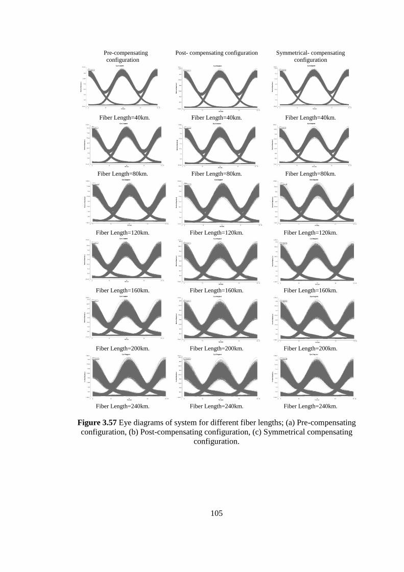
105
Pre-compensating
configuration
Post- compensating configuration
Symmetrical- compensating
configuration
Fiber Length=40km. Fiber Length=40km. Fiber Length=40km.
Fiber Length=80km. Fiber Length=80km. Fiber Length=80km.
Fiber Length=120km. Fiber Length=120km. Fiber Length=120km.
Fiber Length=160km. Fiber Length=160km. Fiber Length=160km.
Fiber Length=200km. Fiber Length=200km. Fiber Length=200km.
Fiber Length=240km. Fiber Length=240km. Fiber Length=240km.
Figure 3.57 Eye diagrams of system for different fiber lengths; (a) Pre-compensating
configuration, (b) Post-compensating configuration, (c) Symmetrical compensating
configuration.
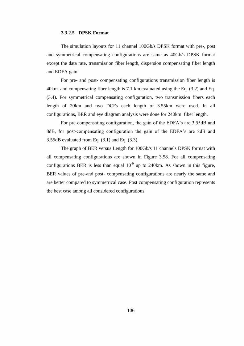
106
3.3.2.5 DPSK Format
The simulation layouts for 11 channel 100Gb/s DPSK format with pre-, post
and symmetrical compensating configurations are same as 40Gb/s DPSK format
except the data rate, transmission fiber length, dispersion compensating fiber length
and EDFA gain.
For pre- and post- compensating configurations transmission fiber length is
40km. and compensating fiber length is 7.1 km evaluated using the Eq. (3.2) and Eq.
(3.4). For symmetrical compensating configuration, two transmission fibers each
length of 20km and two DCFs each length of 3.55km were used. In all
configurations, BER and eye diagram analysis were done for 240km. fiber length.
For pre-compensating configuration, the gain of the EDFA‟s are 3.55dB and
8dB, for post-compensating configuration the gain of the EDFA‟s are 8dB and
3.55dB evaluated from Eq. (3.1) and Eq. (3.3).
The graph of BER versus Length for 100Gb/s 11 channels DPSK format with
all compensating configurations are shown in Figure 3.58. For all compensating
configurations BER is less than equal 10-9
up to 240km. As shown in this figure,
BER values of pre-and post- compensating configurations are nearly the same and
are better compared to symmetrical case. Post compensating configuration represents
the best case among all considered configurations.

107
Figure 3.58 BER versus Length with all dispersion compensating configuration.
The eye diagrams of this system are shown in Figure 3.59. The eye diagrams
show the eye opening of system for different fiber lengths. Each span is 40km. For
all compensating configuration eye opening is good up to 240km.
108
Pre-compensating
configuration
Post- compensating configuration
Symmetrical- compensating
configuration
Fiber Length=40km. Fiber Length=40km. Fiber Length=40km.
Fiber Length=80km. Fiber Length=80km. Fiber Length=80km.
Fiber Length=120km. Fiber Length=120km. Fiber Length=120km.
Fiber Length=160km. Fiber Length=160km. Fiber Length=160km.
Fiber Length=200km. Fiber Length=200km. Fiber Length=200km.
Fiber Length=240km. Fiber Length=240km. Fiber Length=240km.
Figure 3.59 Eye diagrams of system for different fiber lengths; (a) Pre-compensating
configuration, (b) Post-compensating configuration, (c) Symmetrical compensating
configuration.
109
3.3.2.6 CSRZ DPSK Format
The simulation layouts for 11 channel 100Gb/s CSRZ DPSK format with
pre-, post- and symmetrical compensating configurations are same as 40Gb/s CSRZ
DPSK format except the data rate, transmission fiber length, dispersion
compensating fiber length and EDFA gain.
For pre- and post- compensating configurations transmission fiber length is
40km. and compensating fiber length is 7.1 km evaluated using the Eq. (3.2) and Eq.
(3.4). For symmetrical compensating configuration, two transmission fibers each
length of 20km and two DCFs each length of 3.55km were used. In all
configurations, BER and eye diagram analysis were done for 240km. fiber length.
For pre-compensating configuration, the gain of the EDFA‟s are 3.55dB and
8dB, for post-compensating configuration the gain of the EDFA‟s are 8dB and
3.55dB evaluated from Eq. (3.1) and Eq. (3.3).
The graph of BER versus Length for 100Gb/s 11 channels NRZ format with
all compensating configurations are shown in Figure 3.60 For all compensating
configurations BER is less than equal 10-9
up to 240km. As shown in this figure,
BER values of pre-and post- compensating configurations are nearly the same.
Symmetrical compensating configuration represents the best case among all
considered configurations.

110
Figure 3.60 BER versus Length with all dispersion compensating configuration.
The eye diagrams of this system are shown in Figure 3.61. The eye diagrams
show the eye opening of system for different fiber lengths. Each span is 40km. As
seen from this figure eye opening is good up to 240km.

111
Pre-compensating
configuration
Post- compensating configuration
Symmetrical- compensating
configuration
Fiber Length=40km. Fiber Length=40km. Fiber Length=40km.
Fiber Length=80km. Fiber Length=80km. Fiber Length=80km.
Fiber Length=120km. Fiber Length=120km. Fiber Length=120km.
Fiber Length=160km. Fiber Length=160km. Fiber Length=160km.
Fiber Length=200km. Fiber Length=200km. Fiber Length=200km.
Fiber Length=240km. Fiber Length=240km. Fiber Length=240km.
Figure 3.61 Eye diagrams of system for different fiber lengths; (a) Pre-compensating
configuration, (b) Post-compensating configuration, (c) Symmetrical compensating
configuration.

112
11 channels 100Gb/s for all modulation formats with pre- compensating
configuration is shown in Figure 3.62. As shown in this figure, CSRZ DPSK
modulation format represents the best case among all considered formats up to
240km. The performance of RZ is better compared to others up to 200km. CSRZ is
good up to 200km. NRZ and DPSK also provide 240km. CRZ is the worst case.
Figure 3.62 BER versus Length for 11 channels 100Gb/s system for all modulation
formats with pre-compensating configuration.
Figure 3.63 shows the 11 channels 100Gb/s for all modulation formats with
post-compensating configuration. As shown in this figure, CSRZ DPSK modulation
format represents the best case among all considered formats up to 240km. The
performance of RZ is better compared to others up to 200km. CSRZ is good up to
200km. NRZ and DPSK also provide 240km. CRZ is the worst case.

113
Figure 3.63 BER versus Length for 11channels 100Gb/s system for all modulation
formats with post-compensating configuration.
11 channels 100Gb/s for all modulation formats with symmetrical
compensating configuration is shown in Figure 3.64. As shown in this figure, CSRZ
DPSK modulation format represents the best case among all considered formats up
to 240km. The performance of RZ is better compared to others up to 200km. CSRZ
is good up to 200km. NRZ and DPSK also provide 240km. CRZ is the worst case.

114
Figure 3.64 BER versus Length for 11 channels 100Gb/s system for all modulation
formats with symmetrical compensating configuration.

115
Tab
le 3
.2 P
erfo
rman
ce o
f 40 G
b/s
and 1
00G
b/s
WD
M S
yst
ems
wit
h a
ll M
odula
tion F
orm
ats
and C
om
pen
sati
ng C
onfi
gura
tion
.
116
As seen from the Table 3.2, for single channel 40Gb/s system all modulation
formats with all compensating configuration provide transmission length of 960km.
CSRZ DPSK modulation format with symmetrical compensating configuration
represents better performance among all formats and configuration. Its BER value is
1.13E-47.
For 25 Channels with the same data rate, RZ with symmetrical and pre
compensating configurations, CSRZ with symmetrical compensating configuration
and CSRZ DPSK with all compensating configuration provide 960km. CSRZ DPSK
modulation format with symmetrical compensating configuration represents better
performance among all formats and configuration. Its BER value is 8.83E-16.
For single channel 100Gb/s system NRZ with all compensating
configurations, CSRZ with all compensating configurations, DPSK with all
compensating configurations and CSRZ DPSK with all compensating configuration
provide transmission length of 240km. CSRZ DPSK modulation format with
symmetrical compensating configuration represents better performance among all
formats and configuration. Its BER value is 8.88E-15.
For 11 Channels with the same data rate, NRZ with all compensating
configurations, DPSK with all compensating configuration, and CSRZ DPSK with
all compensating configurations provide 240km. CSRZ DPSK modulation format
with symmetrical compensating configuration represents better performance among
all formats and configuration. Its BER value is 1.02E-14.
As a result for the entire system configuration, CSRZ DPSK modulation
format with symmetrical compensating configuration represents better performance
among all formats and configuration.

117
CHAPTER 4
CONCLUSION
Advanced modulation formats play an important role in the design of
networks. In this dissertation, most used modulation formats were reviewed. NRZ,
RZ, CRZ, CSRZ, DPSK, NRZ-DPSK, RZ-DPSK, and CSRZ-DPSK were been
explained and compared. In order to compare and analysis the transmission
performances of modulation formats computer simulation have been performed. The
system performance was monitored by means of eye-diagram. For all systems BER
versus fiber length were analyzed. Firstly single channel for different modulation
formats were focused on.40Gb/s, 100Gb/s data rate were considered. Then, channel
numbers were increased. For 40Gb/s data-rate, 25 channels were used with the
channel spacing of 160GHz (1.28nm) and total capacity was 1Tb/s. For 100Gb/s
data-rate, 11 channels were used with the channel spacing of 400GHz (3.2nm) and
total capacity was 1.1Tb/s. In all cases, simulations were performed in the C-band
(1530nm – 1565nm).
Different fiber types and different modulation formats could affect the system
performance. In this simulations, Standard Single mode fiber (SSMF) was used.
In order to compensate the accumulated dispersion in the fiber different types
of dispersion compensating configurations were considered. Pre-, post-, and
symmetrical dispersion compensating configurations were applied each case. In these
configurations, optical amplifiers after each fiber have been used to compensate for
the span loss. The system performance has been monitored by means of eye-diagram.
BER and system length graphs for all case analyzed. Symmetrical dispersion
compensating configurations for majority of the modulation formats represents better
performance among all compensating configuration because it is the combination of
pre- and post- compensating configurations and provides the advantages of both of
them. The performances of post- and pre- compensating configurations are nearly the
same and post- case is slightly better compared to pre-case.

118
Chromatic dispersion and nonlinear effects of XPM, SPM and FWM are
important constraints for long haul transmission optical system. These are the critical
to the performance of the system. Modulation formats is the important method to
reduce this linear and nonlinear impairments.
The effect of dispersion is increased while the bit rate increases. 40Gb/s
system has better tolerance to dispersion than 100Gb/s system. For example single
channel 40Gb/s system with symmetrical compensating configuration, the best
performance, has BER value of 1.13E-47 at 960km. On the other hand, single
channel 100Gb/s system with symmetrical compensating configuration, the best
performance, has BER value of 8.88E-15 at 240km. In addition 25 channels 40Gb/s
WDM system with symmetrical compensating configuration, the best performance,
has BER value of 8.83E-16 at 960km. while 11 channels 100Gb/s CSRZ DPSK
WDM system with symmetrical compensating configuration, the best performance,
has BER value of 1.02E-14 at 240km. Therefore 40Gb/s system is simulated for the
transmission length of 960km. and fiber span length of 80km, 100Gb/s system is
simulated for the transmission length of 240km. and fiber span length of 40km. In
simulations, maximum transmission length for single and 25 channels 40Gb/s
systems are 960km., for single and 11 channels 100GB/s systems are 240km.
The nonlinear effects of the fiber are increased in multiple channels. The
performance of single channel is better than 25 channels in 40Gb/s system. Similarly,
the performance of single channel is better than 11 channels in 100Gb/s system. For
example, the performance of single channel 40Gb/s CSRZ DPSK system with
symmetrical compensating configuration, the best performance, has BER value of
1.13E-47 at 960km. On the other hand 25 channels of that system has BER value of
8.83E-16 at 960km. The performance of single channel 100Gb/s CSRZ DPSK
system with symmetrical compensating configuration, the best performance, has
BER value of 8.88E-15 at 240km. On the other hand 11 channels of that system has
BER value of 1.02E-14 at 240km. FWM, SPM and XPM decrease the system
performance in multiple channels systems. The single channel is affected by only
SPM nonlinear effect. One way to manage with FWM is to use unequal channel.

119
Another, and very effective, way is fiber dispersion management method. This
method is also effective for SPM and XPM.
In simulations for all configurations input power is 1.0E-3W. When the
power is increased nonlinear effects are increased.
Most commercial systems use the NRZ modulation format. It is easy to
implement, and less costly. The performance of 25 channels 40Gb/s RZ with all
compensating configurations are better compared to 25 channels 40Gb/s NRZ but in
11 channels 100Gb/s system performance of NRZ is better than RZ. For example, 25
channels 40Gb/s NRZ with pre compensating configuration has BER value of
9.49E-9 at 480km. while RZ with pre configuration has BER value of 5.82E-9 at
960km. 11 channels 100Gb/s NRZ with pre compensating configuration has BER
value of 1.09E-12 at 240km. while RZ with pre configuration has BER value of
3.27E-14 at 200km. Because RZ is more tolerant to nonlinearity than NRZ, however,
suffers from a stronger signal degradation due to chromatic dispersion. 100Gb/s
system is less tolerant to dispersion.
CSRZ is special form of RZ where the carrier is suppressed. The dispersion
tolerance of CSRZ modulation can be improved due its reduced spectral width
compared to RZ modulation. For example, single channel 100Gb/s CSRZ system
with symmetrical compensating configuration has BER value of 2.65E-9 at 240km.,
while RZ has BER value of 2.22E-17 at 200km. In addition, carrier suppression
reduces the efficiency of FWM in WDM systems.
DPSK is more tolerant to nonlinear effects. It has better resilience to XPM
and FWM, as compared with intensity modulation formats. For example, 11 channels
100Gb/s DPSK system with post compensating configuration has BER value of
2.71E-13 at 240km., while NRZ has BER value of 6.07E-13 at 240km., RZ has BER
value of 4.44E-14 at 200km.
CSRZ-DPSK exhibit superior transmission performance than simple DPSK.
The CSRZ-DPSK pulses posses a RZ signal shape and due to the reduced spectral
width, CSRZ-DPSK modulation shows an increased dispersion tolerance and it is
more robust to nonlinear impairments than conventional RZ format. In all systems
that simulated the performance of CSRZ DPSK is better than DPSK. For example,

120
11 channels 100GB/s with symmetrical compensating configuration has BER value
of 1.02E-14 at 240km., while DPSK has BER value of 3.13E-12 at 240km.
As a result for all the systems considered in this dissertation, CSRZ DPSK
modulation format with symmetrical compensating configuration represents better
performance among all formats and compensating configurations. For single channel
40Gb/s BER value of CSRZ DPSK with symmetrical compensating configuration is
1.13E-47, for 25 channels 40Gb/s system BER value is 8.83E-16, for single channel
100Gb/s system BER is 8.88E-15, for 11 channels 100Gb/s system BER is 1.02E-14.
The performance of CSRZ DPSK modulation format with other dispersion
compensating configuration is also good.
121
REFERENCES
[1] John M. Senior, Optical Fiber Communications Principles and Practice,
Second Edition, 1992.
[2] Govind P. Agrawal, Fiber Optic Communication Systems, Third edition,
2002.
[3] Le Nguyen Binh, Digital Optical Communications, 2009.
[4] Gerd Keiser, Optical Fiber Communications, Third edition, 2000.
[5] R. Sabella, “Tutorial: Key elements for WDM Transport Networks”,
Photonic Network Communications, 2:1, 7-14, 2000.
[6] Ashwin Gumaste, Tony Antony, DWDM Network Designs and Engineering
Solutions, 2003.
[7] Harold Kolimbiris, Fiber Optics Communications, 2004.
[8] Micheal S. Borella, Jason P. Jue, Dhritiman Banerjee, Byrav Ramamurthy,
and Biswanath Mukherjee, “Optical Components for WDM Lightwave
Networks”, Proceedings of the IEEE, Vol. 85, No.8, August 1997.
[9] Clifford Pallock, Fundamentals of Optoelectronics,1995.
[10] Gabriel Charlet, “Progress in Optical Modulation Formats for High-Bit Rate
WDM Transmissions” IEEE Journal of Selected Topics In Quantum
Electronics, Vol. 12, No. 4, July/August 2006.
[11] Y R Zhou, A Lord and E S R Sikora, “Ultra-long-haul WDM transmission
Systems”, BT Technology Journal, Vol 20, No 4, October 2002.

122
[12] Gerald P. Ryan, Dense Wavelength Division Multiplexing, ATG‟s
Communications &Networking Technology Guide Series, 1997.
[13] Sen Zhang, “Advanced Optical Modulation Formats in High-speed
Lightwave System”, Thesis (M.S.), Department of Electrical Engineering and
Computer Science and the Faculty of the Graduate School of the University
of Kansas, 2004.
[14] Yang Jing Wen, Jinyu Mo, and Yixin Wang, “Advanced Data Modulation
Techniques for WDM Transmission”, IEEE Communications Magazine,
August 2006, 58-65.
[15] Le Nguyen Binh, “MATLAB Simulink Simulation Platform for Photonic
Transmission Systems”, I. J. Communications, Network and System Sciences,
May 2009, 2, 91-168.
[16] Peter J. Winzer, Rene-Jean Essiambre, “Advanced Optical Modulation
Formats”, Proceedings of the IEEE, Vol. 94, No. 5, May 2006, 952-985.
[17] A. Garcia Perez, J.A. Andrade Lucio, O.G. Ibarra Manzano, M. Trejo Duran,
H.Gutierrez Martin, “Efficient Modulation Formats for High Bit-Rate Fiber
Transmission”, Acta Universitaria, mayo-agosto, ano/vol. 16, numero 002,
Universidad de Guanajuato, Mexico, pp. 17-26, 2006.
[18] Anes Hodzic, Beate Konrad, and Klaus Petermann, “Alternative Modulation
Formats in N 40 Gb/s WDM Standard Fiber RZ-Transmission Systems”,
Journal Of Lightwave Technology, Vol. 20, No. 4, April 2002.

123
[19] L.N. Binh and D. Wong, “DWDM Optically Amplified Transmission
Systems-Simulink Models and Test-Bed: PART III –DPSK Modulation
Format”, Monash University, Department of Electrical and Computer
Systems Engineering,Technical Report, 2005.
[20] Ivan P. Kaminow and Tingye Li, Optical Fiber Telecommunications IV-A,
Fourth Edition, 2002.
[21] Ron Hui, Sen Zhang, etc. “Advanced Optical Modulation Formats and Their
Comparison in Fiber-Optic Systems”, A Technical Report to Sprint, by
Lightwave Communication Systems Laboratory, The University of Kansas,
2004.
[22] Muhammad Haris,”Advanced Modulation Formats For High-Bit-Rate Optical
Networks”, Dissertation, .School of Electrical and computer Engineering,
Georgia Institute of Technology, August 2008.
[23] VPItransmissionMakerTM
WDM Manuel.
[24] Siddharth Ramachandran, Optical and Fiber Communications Reports, Fiber
Based Dispersion Compensation, Volume 5, 2007.
[25] Agilent Technologies, “Measuring Jitter in Digital Systems”, Application
Note 1448-1, 2008
[26] Klaus Petermann, Optical Communication Theory and Techniques, 2005.
[27] Pallock C. R, Fundamentals of Optoelectronics, 1995.

124
APPENDIX A
Figure A.1 Simulation set up of 10 Gb/s NRZ modulation.
Figure A.2 Simulation set up of 10 Gb/s RZ modulation.

125
Figure A.3 Simulation set up of 10 Gb/s CRZ modulation.
Figure A.4 Simulation set up of 10 Gb/s CSRZ modulation.

126
Figure A.5 Simulation set up of 10 Gb/s DPSK modulation.
Figure A. 6 Simulation set up of 10 Gb/s CSRZ DPSK modulation.
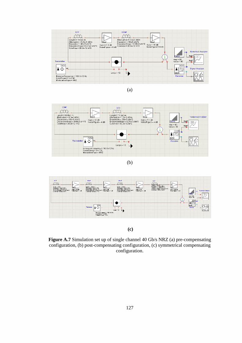
127
(a)
(b)
(c)
Figure A.7 Simulation set up of single channel 40 Gb/s NRZ (a) pre-compensating
configuration, (b) post-compensating configuration, (c) symmetrical compensating
configuration.
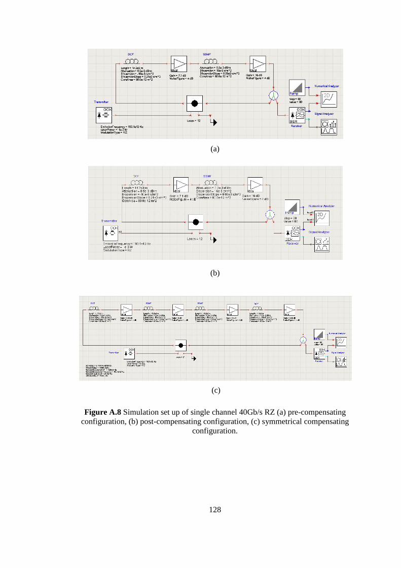
128
(a)
(b)
(c)
Figure A.8 Simulation set up of single channel 40Gb/s RZ (a) pre-compensating
configuration, (b) post-compensating configuration, (c) symmetrical compensating
configuration.
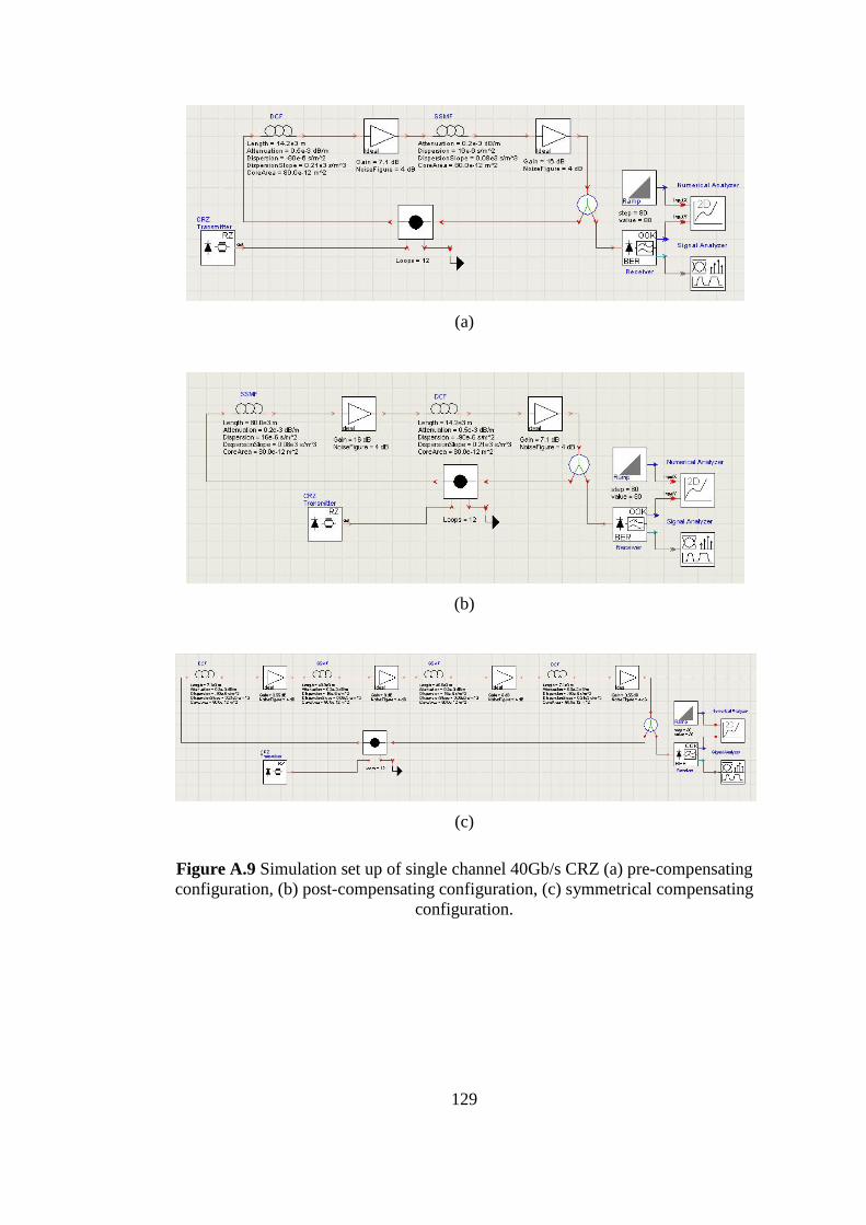
129
(a)
(b)
(c)
Figure A.9 Simulation set up of single channel 40Gb/s CRZ (a) pre-compensating
configuration, (b) post-compensating configuration, (c) symmetrical compensating
configuration.

130
(a)
(b)
(c)
Figure A.10 Simulation set up of single channel 40Gb/s CSRZ (a) pre-compensating
configuration, (b) post-compensating configuration, (c) symmetrical compensating
configuration.

131
(a)
(b)
(c)
Figure A.11 Simulation set up of single channel 40Gb/s DPSK (a) pre-compensating
configuration, (b) post-compensating configuration, (c) symmetrical compensating
configuration.

132
(a)
(b)
(c)
Figure A. 12 Simulation set up of single channel 40Gb/s CSRZ-DPSK (a) pre-
compensating configuration, (b) post-compensating configuration, (c) symmetrical
compensating configuration.

133
(a)
(b)
(c)
Figure A.13 Simulation set up of 25 channels 40Gb/s NRZ (a) pre-compensating
configuration, (b) post-compensating configuration, (c) symmetrical compensating
configuration.

134
(a)
(b)
(c)
Figure A.14 Simulation set up of 25 channels 40Gb/s RZ (a) pre-compensating
configuration, (b) post-compensating configuration, (c) symmetrical compensating
configuration.

135
(a)
(b)
(c)
Figure A.15 Simulation set up of 25 channels 40Gb/s CRZ (a) pre-compensating
configuration, (b) post-compensating configuration, (c) symmetrical compensating
configuration.

136
(a)
(b)
(c)
Figure A.16 Simulation set up of 25 channels 40Gb/s CSRZ (a) pre-compensating
configuration, (b) post-compensating configuration, (c) symmetrical compensating
configuration.

137
(a)
(b)
(c)
Figure A. 17 Simulation set up of 25 channels 40Gb/s DPSK (a) pre-compensating
configuration, (b) post-compensating configuration, (c) symmetrical compensating
configuration.

138
(a)
(b)
(c)
Figure A. 18 Simulation set up of 25 channels 40Gb/s CSRZ-DPSK (a) pre-
compensating configuration, (b) post-compensating configuration, (c) symmetrical
compensating configuration.

139
CURRICULUM VITAE
PERSONAL INFORMATION
Surname, Name: Büyükşahin Öncel, F. Feza
Nationality: Turkish (TC)
Date and Place of Birth: 11 September 1975 , Ankara
Marital Status: Married
Phone: +90 312 266 37 65
Fax: +90 312 266 37 64
email: [email protected]
EDUCATION
Degree Institution Year of Graduation
MS METU Physics 2001
BS METU Physics 1997
High School Yahya Kemal Beyatlı Lisesi, Ankara 1992
WORK EXPERIENCE
Year Place Enrollment
2007-Present STM Savunma Teknolojileri Mühendislik A.Ş Systems Engineer
Consultant
2003-2007 Maliye Bakanlığı
Bütçe ve Mali Kontrol Genel Müdürlüğü System Analysts
1997-2003 Başbakanlık Aile Araştırma Kurumu System Analysts
1998-1999 Data Kontrol Instructors
Bilgisayar Sanayi ve Ticaret Ltd. Şti.
1997 METU Computer Center Computer Operator
FOREIGN LANGUAGES
Fluent English, Basic Japanese

140
PARTICIPATED SCIENTIFIC MEETINGS AND CONGRESS
Elektronik Harp Konferansı May 2009
Savunma Sanayi Müsteşarlığı, Ankara
Radar Sistemlerinde Mevcut Kabiliyetler Çalıştayı March 2009
Savunma Sanayi Müsteşarlığı, Ankara
UZAL CBS 2008 II. Uzaktan Algılama ve Coğrafi Bilgi Sistemleri Oct 2008
Erciyes Ü. Kayseri,
“Helikopterler için Engel Tespit ve Uyarı Sistemleri” (Paper presentation)
SPIE Defense & Security Conference March 2008
SPIE, USA
6th National Optic Electro-Optic and Photonic Meeting Dec 2004
Sabancı University, İstanbul
5th National Optic Electro-Optic and Photonic Meeting Dec 2003
METU, Ankara
4th National Optic Electro-Optic Meeting Dec 2002
TÜBITAK-UME, Gebze
3rd National Electro-Optic Meeting Nov 2001
ASELSAN Electronic Industries Inc., Ankara
"Simulation on 4 x 2.5 Gbit/s WDM System." (Poster presentation)
TURKISH PHYSICAL SOCIETY 19th PHYSICS CONFERENCE Sept 2000
Fırat University, Elazığ
HOBBIES
Tennis, Computer Technologies, Movies.


![2 3 4 5 void ordered_fill (float* array, int array_length) { int index; for (index = 0; index < array_length; index++) { array[index] = index; }](https://img.pdfslide.us/doc/110x75/56649e0d5503460f94af6e07/2-3-4-5-void-orderedfill-float-array-int-arraylength-int-index-for.jpg)


![767 INDEX [] · 767 INDEX ... index](https://img.pdfslide.us/doc/110x75/5e6407d785e377181b6fee19/767-index-767-index-index-.jpg)

![INDEX [] · 2019-04-15 · INDEX ... index](https://img.pdfslide.us/doc/110x75/5e5bc6adf543e8499e5ad9a4/index-2019-04-15-index-index.jpg)


![Index [] · viii Index Acknowledgement .....i](https://img.pdfslide.us/doc/110x75/5fca3a2414492b06193f3864/index-viii-index-acknowledgement-i.jpg)