Department of Physics

Seminar Ib – 1st year, 2nd cycle

Independent Component Analysis

Author: Žiga Zaplotnik

Advisor: prof. dr. Simon Širca

Ljubljana, April 2014

Abstract

In this seminar we present a computational method for blind signal separation. Its

purpose is to deduce source signals from a set of various mixed signals without

any information about the source signals or mixing process. Independent

component analysis is a recently developed method in which the goal is to find

source components which are statistically independent, or as independent as

possible. We give a description of the basic concepts of this method based on

cocktail-party problem example. We also discuss its implementation. Finally, we

present some already used applications of independent component analysis.

2

Contents

1 Introduction 2

2 Principles of ICA estimation 4

2.1 Definition of ICA model ................................................................................. 4

2.2 Constraints..................................................................................................... 6

2.3 Estimating ICA model by maximizing non-Gaussianity .................................... 7

2.4 Ambiguities of ICA ........................................................................................ 8

3 Applications of ICA 9

3.1 Electrocardiography ......................................................................................10

3.2 Reflection Cancelling ....................................................................................11

4 Conclusions 12

References 12

1 Introduction

Independent component analysis (ICA) is a statistical computational method for blind

signal (source) separation – that means separation of source signals (audio, speech,

image, geophysical, medical...) from a set of mixed signals. Term 'blind' suggests that

there is little or no information about the signals or mixing process.

ICA was first introduced in 1986 by Herault and Jutten [1]. Comon provided the most

widely used mathematical definition of ICA in 1994 [2]. We will give a more detailed

description of it in the next chapter. First fast and efficient ICA algorithm was introduced

by Bell and Seynowski in 1995 [3]. From then on many different ICA algorithms were

published. One of the most used, including in industrial applications (which we will

discuss in the last chapter) is the FastICA algorithm, developed by Hyvärinen and Oja

in 1999 [4,5,6].

As the name implies, the basic goal of ICA is to estimate such a transformation of an

observed mixture of signals, that the resulting source components are minimally

correlated or as independent as possible in a probabilistic sense. Furthermore, the signals

have to be non-Gaussian. For example, we measure signals ( ), ( ) of two

microphones recording the speech of two persons (sources) ( ) and ( ). We assume

that each source reaches both microphones at the same time (there is no time/phase

delay). That means that the distance between microphones has to be much smaller than

the source signal wavelength . However, it is important that the microphones amplify

more the signals coming from certain directions (like our ears do), otherwise the

measured signals ( ) are all the same. So we can assume that each of these recorded

3

signals is a weighted sum (linear combination) of the speech signals. We could express

this as a linear equation

( ( )

( )) (

)( ( )

( )) (1)

which holds for every timestamp . Here, both sources and matrix elements are

unknown. The value of depends on the relative contribution of the source signal to

recorded mixture .

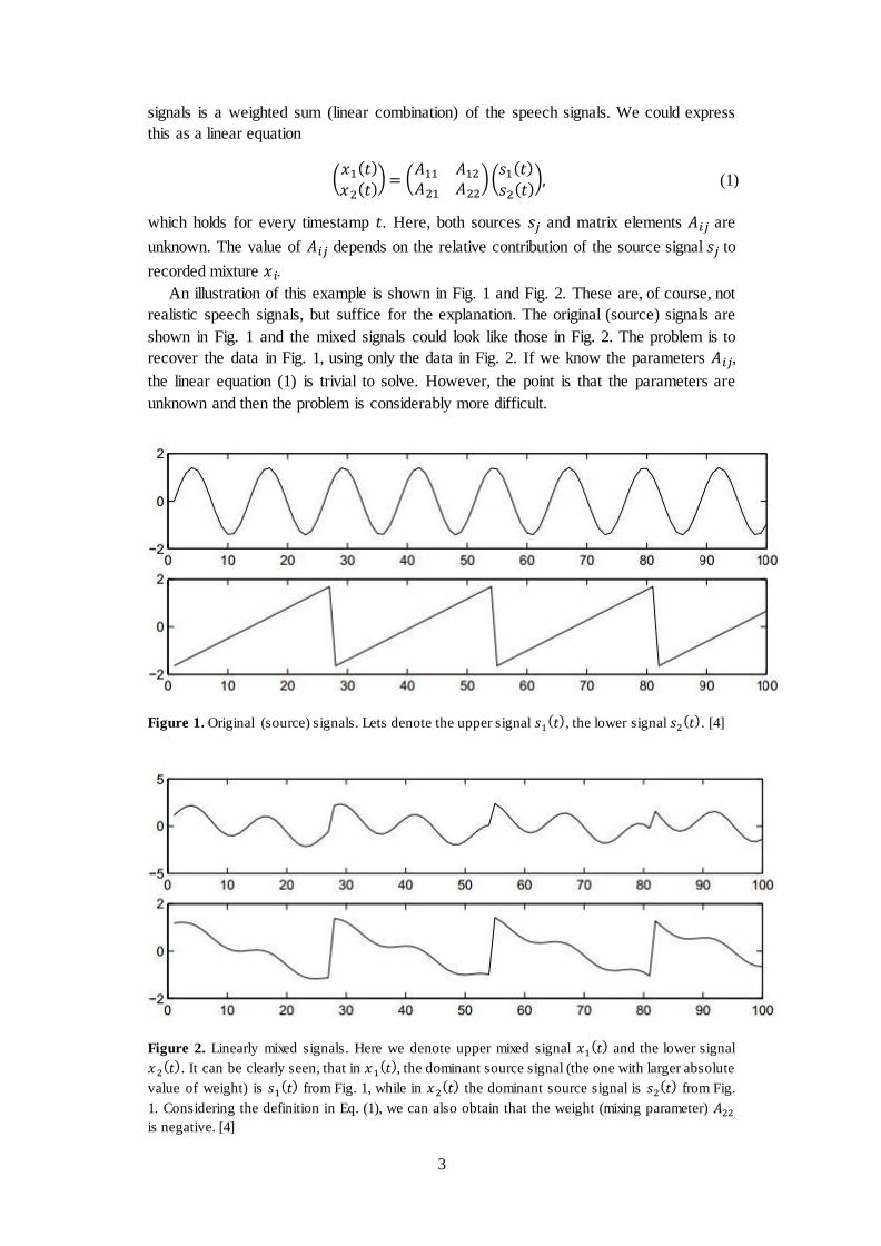
An illustration of this example is shown in Fig. 1 and Fig. 2. These are, of course, not

realistic speech signals, but suffice for the explanation. The original (source) signals are

shown in Fig. 1 and the mixed signals could look like those in Fig. 2. The problem is to

recover the data in Fig. 1, using only the data in Fig. 2. If we know the parameters ,

the linear equation (1) is trivial to solve. However, the point is that the parameters are

unknown and then the problem is considerably more difficult.

Figure 1. Original (source) signals. Lets denote the upper signal ( ), the lower signal ( ). [4]

Figure 2. Linearly mixed signals. Here we denote upper mixed signal ( ) and the lower signal

( ). It can be clearly seen, that in ( ), the dominant source signal (the one with larger absolute

value of weight) is ( ) from Fig. 1, while in ( ) the dominant source signal is ( ) from Fig.

1. Considering the definition in Eq. (1), we can also obtain that the weight (mixing parameter)

is negative. [4]

4

The above example is an example of the famous cocktail-party problem, a problem

related to cocktail-party effect. The cocktail-party effect is the phenomenon of being able

to focus attention on a particular stimulus while filtering out other stimuli. For example

one is able to focus on a single conversation in a noisy room. However, this requires

hearing with both ears. People with only one functioning ear are much more distracted by

interfering noise than people with two healthy ears. The reason is following: the auditory

system (sensory system for the sense of hearing) has to be able to localize and process at

least two sound sources in order to extract the signals of one sound source out of a

mixture of interfering sound sources. Here localizing means turning head into the

direction of the source of interest and so amplifying the signal coming from it [7].

A similar condition occurs in ICA – a number of obseved sound mixtures must be at

least as large as the number of independent sound components. Algortihm alone ofcourse

cannot localize (and so amplify) certain signals, therefore only two microphones in a

room of three simultaneously speaking people are insufficient in order to separate sound

signals of all three speakers.

Here, we started a discussion about conditions and limits of ICA. In the next section

we describe a generalized cocktail-party problem. In order to be able to solve this

problem we also give a detailed insight into the ideas and construction of ICA.

2 Principles of ICA estimation

2.1 Definition of ICA model

Here we only describe noiseless linear independent component analysis. Assume that we

observe linear mixtures of independent components (sources) .

Then we can define the ICA model

(2)

where is the mixing matrix. ICA model (2) describes how the observed data

are generated by a process of mixing the components (sources). We have now dropped

the time index as (2) holds at any given time instant. With the purpose of efficiently

describing ICA, we rather work with random variables instead of the proper time signals

from here on. That means we assume each mixture as well as each independent

component is a random variable, instead of the amplitude of the signal at certain time .

We neglect measurement errors, which could (in case they exist) be added to the right

side of (2). We assume that noise is already included in the sources . So there is also no

noise at the right side of (2) – as we said, we are performing noiseless ICA. We also

assume that the signal is centered (random variables have zero mean or ⟨ ⟩ ) and

that the variables are of unit variance: ⟨ ⟩ .

Let us now illustrate the ICA model in statistical terms. Consider two independent

components , with uniform distributions

( ) {

√ | | √

(3)

5

The range of values for this uniform distribution were chosen so as to make the mean

zero and the variance equal to one, in accordance with the preceding paragraph. Joint

probabilty density of and is then uniform on a square, as shown in Fig. 3. Now let

us mix these two independent components with the following mixing matrix

(

) (4)

The mixing gives us two mixed variables, and . Now, the mixed data has a uniform

distribution on a parallelogram (also shown in Fig. 3). But random components and

are not independent any more. This can be clearly seen if we are trying to predict the

value of one of them, for example , based on the value of the other, . For example,

when attains maximum or minimum value, then this completely determines the value

of . That means they are not independent.

Figure 3. [LEFT] The joint distribution of the independent source components and with

uniform distributions. Horizontal axis: , vertical axis: . [RIGHT] The joint distribution of the

observed mixtures and . Variables and are not independent any more. For example,

when taking maximum or minimum value of , variable is uniquely determined by .

Horizontal axis: , vertical axis: . [4]

Our main task is to reconstruct sources based on the observed . We have no

information about the mixing process by matrix . However, if the matrix is of full

rank, a separation or unmixing matrix exists. Then unmixing process can be written as

( ) ( ) (5)

Here are the rows of . We attempt to find an estimate of the separation matrix so

that we can reconstruct . In order to estimate matrix , several additional requirements

(conditions) should be fulfilled. The constraints for the validity and possibility of solving

blind signal separation problem with ICA method are discussed in the next section.

6

2.2 Constraints

Here we describe three important constraints for ICA method to be valid.

1) The problem is well- or over-determined. The number of measured signals has to

be equal to or greater than the number of source signals ( ). Otherwise it is

impossible to separate the sources using ICA alone.

2) Mixing is instantenous. No delay is permitted between the time each source signal

reaches sensors/microphones/observers/recording stations located in different places.

In order to avoid (time) delay, recorded signals are aligned using the cross-correlation

function (sliding dot product; similar to convolution). For continuous signals and ,

it is defined as

( )( ) ∫ ( ) ( )

(6)

If and are functions that differ only by an unknown shift along the -axis, then

cross-correlation can be used to find how much must be shifted along the -axis to

align with . When the functions match, the value of ( ) is maximized.

3) Statistical independance of sources. The independence of variables is

mathematically expressed by the statement that their joint probability density is

factorizable in the following way: ( ) ( ) ( ) ( ). Basically

the variables are said to be independent if information on the value of does

not give any information on the value of , and vice versa. A pair of statistically

independent variables ( ) is uncorrelated and has the covariance ( )

⟨ ⟩ ⟨ ⟩⟨ ⟩ . Uncorrelatedness is a weaker form of independence: if the

variables are independent, they are uncorrelated, but the opposite is not necessary

true. The source signals must be statistically independent or as independent as

possible. This is difficult to verify in advance because distribution of data is not

available in real world problems.

4) Source signals must be non-Gaussian (except one signal) . (Fig. 4) This is the

fundamental restriction of ICA to be possible. Here is an explanation, why more than

one Gaussian variable make ICA impossible. Assume that the mixing matrix is

orthogonal and the variables and are Gaussian. Then and are Gaussian too

and their joint probability density is Gaussian again

( )

(

) (7)

The probabilty density is perfectly symmetric (Fig. 4) and so it does not contain any

information on the directions of the columns of the mixing matrix . That means

matrix cannot be estimated. One can prove, that the distribution of any orthogonal

transformation of the gaussian variables ( ) has exactly the same distribution as

( ) and that and are still independent. Thus, in the case of more than one

Gaussian variable, we can only estimate up to an orthogonal transformation and the

matrix is not identifiable. But if only one independent component is Gaussian, ICA

7

is still possible. Non-Gaussianity is the key to estimating the ICA model, as we will

see in the next section.

Figure 4. [LEFT] The comparison between probabilty density function of Gaussian and non -

Gaussian signal. [RIGHT] The joint multivariate distribution of two independent Gaussian

variables (Eq. 6). Horizontal axis: , vertical axis: .

2.3 Estimating ICA model by maximizing non-Gaussianity

First, we denote one-dimensional projections of the observed signals :

(8)

where are the vectors to be determined. If one were one of the rows of the

generalized inverse (separation matrix) of , this linear combination would actually

equal to one of the independent components, . Now the question is how to

determine so that it would equal one of the rows in unmixing matrix . We can show

from (2) and (8) that this relation holds:

∑

(9)

That means that is a linear combination of with weights . Now we use a

statement that comes from the Central Limit Theorem – 'a sum of two independent

random variables has a distribution that is closer to Gaussian than a distribution of any of

the two original random variables'. In our case, that implies that is more Gaussian than

any of the in the linear combination (9). Therefore becomes least Gaussian when it

in fact equals one of the independent components (which means that only one of the

elements of is nonzero). That means we would take as a vector that minimizes

Gaussianity or maximizes non-Gaussianity of [4]. In practice, we would start

with some vector , compute the direction, in which non-Gaussianity is growing most

strongly based on the observed mixture vector , and use some gradient method (for

example Newton's method) for finding a new vector . The whole algorithm is beyond

the scope of this seminar but can be found in [5].

8

To maximize non-Gaussianity, first, we must have a measure of non-Gaussianity. The

classical measure (because of computational simplicity) for non-Gaussianity of a

continuous random variable is the absoulute value of kurtosis

| ( )| |⟨ ⟩ ⟨ ⟩ | (10)

which is a fourth order cumulant of probability distribution. For Gaussian random

variable, the kurtosis is zero. However, practically (when estimated from a measured

sample), curtosis is not robust as it is very sensitive to outliers. Its value may strongly

depend on only a few observations in the tails of the distribution, which may not be

correct at all. The difference between Gaussian distribution and the distribution of

could then rather be measured by Shannon (information) entropy

( ) ∫ ( ) ( ) (11)

where ( ) is the probabilty density function of . The more unpredictable the variable

is, the larger its entropy. An important result of information theory is that 'a Gaussian

variable has the largest entropy among all random variables of equal variance' [8]. This

means entropy could be used as a measure of non-Gaussianity. It turns out, that it is more

practical to work with negentropy

( ) ( ) ( ) (12)

which is zero for a Gaussian variable and positive otherwise. The problem of using

negentropy as a measure of non-Gaussianity is that ( ) from (11) is not known in

advance and that it is computationally very difficult. We therefore use approximations of

negentropy, most often

( ) [⟨ ( )⟩ ⟨ ( )⟩] (13)

where ( ) is a non-quadratic function of . The following choices of have proved

useful [4]: ( )

and ( ) (

), where .

2.4 Ambiguities of ICA

By looking at (2), it is obvious that the following ambiguities will hold (Fig. 5):

1) Variances (energies) of the independent components cannot be determined.

Vector of sources and the mixing matrix are both unknown. That means that any

scalar multiplier of the source could always be cancelled by dividing the

corresponding column of by the same scalar. So the magnitudes (amplitudes) of

the independent components are unknown.

2) Sign ambiguity. We could multiply any independent component by (phase

reversal) without affecting the model.

3) Order of independent components cannot be determined. The estimated source

signals may be recovered in different order. The reason is again that both and are

unknown.

9

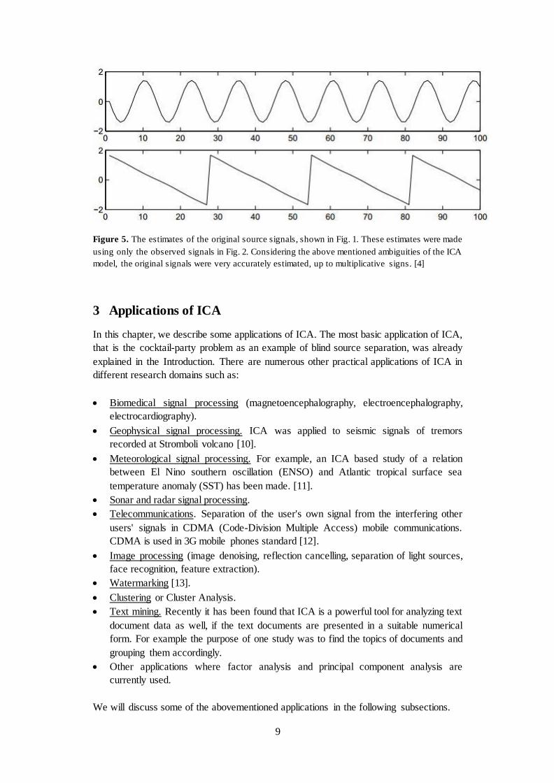
Figure 5. The estimates of the original source signals, shown in Fig. 1. These estimates were made

using only the observed signals in Fig. 2. Considering the above mentioned ambiguities of the ICA

model, the original signals were very accurately estimated, up to multiplicative signs. [4]

3 Applications of ICA

In this chapter, we describe some applications of ICA. The most basic application of ICA,

that is the cocktail-party problem as an example of blind source separation, was already

explained in the Introduction. There are numerous other practical applications of ICA in

different research domains such as:

Biomedical signal processing (magnetoencephalography, electroencephalography,

electrocardiography).

Geophysical signal processing. ICA was applied to seismic signals of tremors

recorded at Stromboli volcano [10].

Meteorological signal processing. For example, an ICA based study of a relation

between El Nino southern oscillation (ENSO) and Atlantic tropical surface sea

temperature anomaly (SST) has been made. [11].

Sonar and radar signal processing.

Telecommunications. Separation of the user's own signal from the interfering other

users' signals in CDMA (Code-Division Multiple Access) mobile communications.

CDMA is used in 3G mobile phones standard [12].

Image processing (image denoising, reflection cancelling, separation of light sources,

face recognition, feature extraction).

Watermarking [13].

Clustering or Cluster Analysis.

Text mining. Recently it has been found that ICA is a powerful tool for analyzing text

document data as well, if the text documents are presented in a suitable numerical

form. For example the purpose of one study was to find the topics of documents and

grouping them accordingly.

Other applications where factor analysis and principal component analysis are

currently used.

We will discuss some of the abovementioned applications in the following subsections.

10

3.1 Electrocardiography

Routinely recorded electro-cardiograms (ECGs) are often corrupted by different types of

artifacts. The term 'artifact' comes from word artificial – that means that it is recorded

from sources other than the electronic signals of the heart. Examples of artifacts in ECGs

are electrical interference from a nearby electrical appliance, patient's muscle tremors as a

result of movements, speaking, deep respiration etc.

The presence of artifacts in the ECGs is very common and the knowledge of them is

necessary to prevent misinterpretation of a heart's rhythm which can lead to wrong

diagnoses. Even better is to almost completely remove noise and artefacts from ECGs.

This can be done with ICA [14]. Here, an important difficulty is one of the ICA

ambiguities – determination of the order of the independent components. That means that

still a trained physician is needed to manually interpret the deduced independent

components.

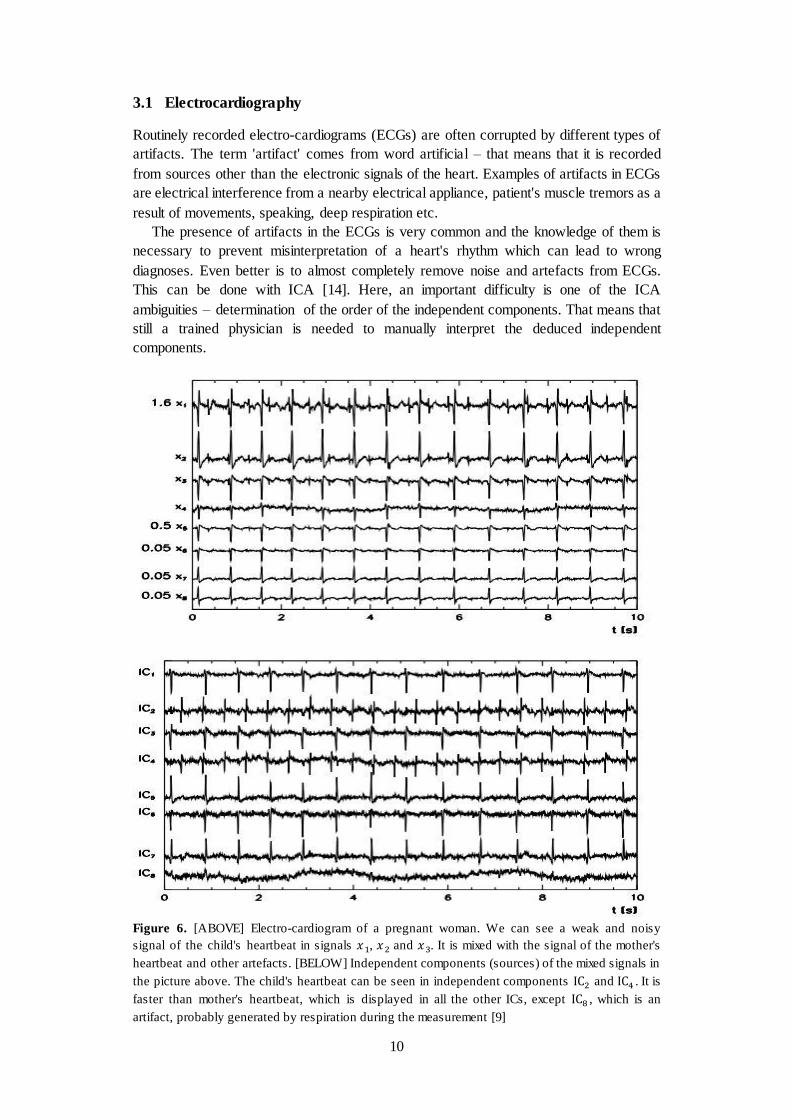
Figure 6. [ABOVE] Electro-cardiogram of a pregnant woman. We can see a weak and noisy

signal of the child's heartbeat in signals , and . It is mixed with the signal of the mother's

heartbeat and other artefacts. [BELOW] Independent components (sources) of the mixed signals in

the picture above. The child's heartbeat can be seen in independent components and . It is

faster than mother's heartbeat, which is displayed in all the other ICs, except , which is an

artifact, probably generated by respiration during the measurement [9]

11

3.2 Reflection Cancelling

When we take a picture through a window, the observed image is often a linear

superposition of two images: the image of the scene beyond the window and the image of

the scene reflected by window. In such cases we cannot view clearly a scene due to

reflections from dielectric surfaces (e.g. glass). Since reflections off a semireflecting

medium such as a glass window at some angle are partially polarized, the strength of the

reflection can be manipulated with a polarizer. However the reflection can only be

completely eliminated when the viewing angle and the incident light direction are in

particular configuration called the Brewster angle. By using images obtained through a

linear polarizer at two or more orientations and applying ICA to them, we can completely

separate reflections [15].

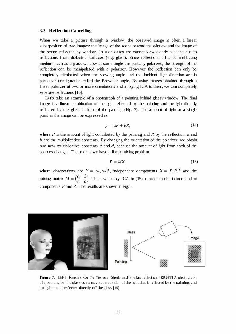
Let's take an example of a photograph of a painting behind glassy window. The final

image is a linear combination of the light reflected by the painting and the light directly

reflected by the glass in front of the painting (Fig. 7). The amount of light at a single

point in the image can be expressed as

(14)

where is the amount of light contributed by the painintg and by the reflection. and

are the multiplicative constants. By changing the orientation of the polarizer, we obtain

two new multiplicative constants and , because the amount of light from each of the

sources changes. That means we have a linear mixing problem

(15)

where observations are [ ] , independent components [ ] and the

mixing matrix (

). Then, we apply ICA to (15) in order to obtain independent

components and . The results are shown in Fig. 8.

Figure 7. [LEFT] Renoir's On the Terrace, Sheila and Sheila's reflection. [RIGHT] A photograph

of a painting behind glass contains a superposition of the light that is reflected by the painting, and

the light that is reflected directly off the glass [15].

12

Figure 8. [LEFT] A pair of images of Renoir's On the Terrace with a reflection of Sheila

photographed through a linear polarizer at orthogonal orientations. [RIGHT] A pair of ICs [15].

4 Conclusions

We have seen that ICA is a very general purpose and applicative computational method

with an almost unlimited potential for future use. Unfortunately, for now, the ICA method

is restricted to linear and barely nonlinear problems. However, the research on the field of

independent component analysis is still very active nowadays, which gives hope for

further improvements of the method and its algorithmic implementations.

References

[1] J. Herault and C. Jutten, Signal Processing 24, 1-10 (1986).

[2] P. Comon, Signal Processing 36, 287-314 (1994).

[3] A.J. Bell and T.J. Sejnowski, Neural Computation 7, 1004-1034 (1995).

[4] A. Hyvärinen and E. Oja, Neural Networks 13, 411-430 (2000)

[5] A. Hyvärinen, IEEE Trans. Neural Networks 10, 626-634 (1999).

[6] A. Hyvärinen, Neural Computing Surveys 2, 94-128 (1999).

[7] J.B. Fritz, M. Elhilali, Curr. Opin. Neurbiol 17, 437-455 (2007).

[8] A. Papoulis, Probability, Random Variables and Stochastic Processes, 3rd edn.

(McGraW-Hill, New York, 1991).

[9] S. Širca, A. Horvat, Computational Methods for Physicists (Springer-Verlag, 2012).

[10] A.Ciaramella, Nonlinear Processes in Geophysics 11, 453-461 (2004).

[11] F. Aires, A. Chedin and J.P. Nadal, J. Geophys. Res. 105 (D13), 17437 (2000).

[12] T. Ristaniemi, J. Joutsensalo, Signal Processing 82, 417-431 (2002).

[13] S. Bounlong, D. Lowe, D. Saad, Journal of Machine Learning 4, 1471-1498 (2003).

[14] T. He, G. Clifford and L. Tarassenko. Neural Comput. & Applic 15, 105-116 (2006).

[15] H. Farid and E.H. Adelson. IEEE Comp. Soc. Conf. on Comp. Vis. and Patt. Rec. 1,

262-267 (1999).