Independence in CLP Languages

MARIA GARCIA DE LA BAN DA

Monash University

MANUEL HERMENEGILDO

Technical University of Madrid (UPM)

and

KIM MARRIOTT

Monash University

Studying independence of goals has proven very useful in the context of logic programming. In particular, it has provided a formal basis for powerful automatic parallelization tools, since independence ensures that two goals may be evaluated in parallel while preserving correctness and efficiency. We extend the concept of independence to constraint logic programs (CLP) and prove that it also ensures the correctness and efficiency of the parallel evaluation of independent goals. Independence for CLP languages is more complex than for logic programming as search space preservation is necessary but no longer sufficient for ensuring correctness and efficiency. Two additional issues arise. The first is that the cost of constraint solving may depend upon the order constraints are encountered. The second is the need to handle dynamic scheduling. We clarify these issues by proposing various types of search independence and constraint solver independence, and show how they can be combined to allow different optimizations, from parallelism to intelligent backtracking. Sufficient conditions for independence which can be evaluated "a priori" at run-time are also proposed. Our study also yields new insights into independence in logic programming languages. In particular, we show that search space preservation is not only a sufficient but also a necessary condition for ensuring correctness and efficiency of parallel execution.

Categories and Subject Descriptors: D.1.2 [Programming Techniques]: Automatic Program­ming—automatic analysis of algorithms; program transformation; D.1.3 [Programming Tech­niques]: Parallel Programming; D.1.6 [Programming Techniques]: Logic Programming; F.3.1 [Logics and Meanings of Programs]: Specifying and Verifying and Reasoning about Pro­grams—Logics of programs

General Terms: Languages, Performance

Additional Key Words and Phrases: Constraint logic programming, independence, parallelism

Authors' addresses: M. Hermenegildo, Universidad Politecnica de Madrid, Facultad de Informati-ca, Madrid, Spain; email: herme@fi.upm.es; M. Garcia de la Banda and K. Marriott, Monash Uni­versity, Computer Science, Melbourne, Australia; email: jmbanda,marriott}<Qcs.monash.edu.au.

1. INTRODUCTION

The notion of independence of program statements or procedure calls is relatively well understood in the context of imperative languages, where several definitions of independence, ranging from those based on the Bernstein conditions to more recent notions of "semantic independence," have been defined and applied primarily in pro­gram parallelization [Bacon et al. 1994; Best and Lengauer 1990]. Independence has also been studied and proved to be a very useful concept in traditional logic pro­gramming. Again, the primary motivation is program parallelization [Hermenegildo and Rossi 1995; Haridi and Janson 1990]. However, it also provides a theoretical basis for other powerful program optimizations, including intelligent backtracking [Pereira and Porto 1982], and goal reordering [Warren and Pereira 1982].

The general, intuitive notion of independence in logic programming is that a goal q is independent of a goal pifp does not "affect" q. A goal p is understood to affect another goal q if p changes the execution of q in an "observable" way. Observables include changing the solutions that q produces ("correctness") and changing the time that it takes to compute such solutions ("efficiency"). This contrasts with more traditional notions of independence which, because of the characteristics of imperative or functional languages, only need to deal with the preservation of cor­rectness [Hermenegildo 1997].

Previous work in the context of traditional logic programming languages [Conery 1983; DeGroot 1984; Hermenegildo and Rossi 1995; Chassin and Codognet 1994] has concentrated on defining sufficient conditions which ensure that goals can be safely executed in parallel. This has been achieved by ensuring that either the goals do not share variables (strict independence) or if they share variables, that they do not "compete" for their bindings (nonstrict independence).

In this paper we consider independence in the general context of the constraint logic programming (CLP) paradigm [Jaffar and Lassez 1987], which has emerged as the natural combination of the constraint solving and logic programming paradigms. As for logic programming, our main motivation is to find conditions which allow goals to be executed in parallel. However, we shall also investigate other types of independence, each of which is "interesting" for a certain class of program trans­formations.

Generalizing the independence results obtained for logic programming to CLP is difficult for two reasons. The first reason is that the cost of constraint solving may depend upon the order in which constraints are encountered. This means we need to introduce a notion of "constraint solver independence" which captures how sensitive the solver is to reordering of constraints. This issue did not arise for logic programs because the standard unification algorithm, as usually implemented, is, in most practical cases, independent in this sense. However, in the more general context of CLP, constraint solver independence need not hold. The second reason is that many CLP languages provide dynamic scheduling of literals in goals. This is useful because it facilitates definition or extension of constraint solvers but is considerably more difficult to understand than the standard left-to-right evaluation of goals in logic programs. Actually, dynamic scheduling is also present in some logic programming languages, but since it is not widely used it has been ignored in work on parallelization. However, it must be addressed in the CLP context because of its importance when writing constraint solvers.

Generalizing independence to arbitrary CLP languages and constraint solvers is not only interesting in itself, but also yields new insights into independence even for logic programs. First, it allows us to simplify many of the earlier results by couching them in terms of constraints rather than substitutions. Second, extension of the results to the case of dynamic scheduling has required us to precisely formalize search space preservation and its relationship to independence.

We believe that generalization of independence to CLP will be useful, since the associated optimizations performed in the context of logic programming appear equally applicable to the context of constraints. Indeed, the cost of performing constraint satisfaction makes the potential performance improvements even larger. Preliminary experiments with and-parallelization of CLP [Garcia de la Banda et al. 1996] provide some evidence in this direction.

The rest of the paper proceeds as follows. Section 2 reviews various models for the parallel execution of logic programs and the associated notions of independence. Section 3 formally defines a parallel execution model for CLP programs. Section 4 clarifies the relationship between search space preservation and the safety of parallel execution. Section 5 presents several concepts of independence for CLP, each one useful for a class of applications and relates these to search space preservation. Section 6 gives sufficient conditions that are easier to detect at run-time than the definitions of independence. Section 7 discusses the notion of independence for CLP at the solver level and discusses additional characteristics required of the solvers, offering some examples. Section 8 extends these results to CLP languages that provide dynamic scheduling. Finally, Section 9 presents our conclusions.

2. INDEPENDENCE FOR PARALLELIZATION IN LOGIC PROGRAMS REVISITED

2.1 Operational Semantics of Logic Programs

In this section we introduce some basic concepts and notation regarding logic pro­grams. We will follow mainly [Apt 1990; Lloyd 1987]. Note that we will only deal with definite logic programs (also referred to as positive logic programs). Also note that while the math italics font will be used for definitions and theorems to represent general objects, the teletype font will be used for representing particular instances of the objects, such as those coming from an example program.

An atom has the form p(x) where x is a sequence of distinct variables and p is a predicate symbol. An equation has the form t = u where t and u are terms. A literal is an atom or an equation. A clause or rule has the form h <— &i, • • • ,bn with n > 0, where h is an atom called the head and b\, • • •, bn is a sequence of literals called the body. A program is a set of rules. A goal is a sequence of literals. The empty literal sequence is denoted by nil, and often omitted. We let vars(t) denote the set of variables occurring in a syntactic expression t. A syntactic expression t is ground if vars(t) = 0. The local variables of the clause h <— b\, • • •, bn are those variables appearing in the body but not in the head, i.e., (vars(bi)U- • -\Jvars(bn))\vars(h).

A renaming is a bijective mapping from variables to variables. We naturally extend renamings to mappings between syntactic objects. Syntactic objects s and s' are said to be variants if there is a renaming such that p(s) = s' where = denotes syntactic equivalence.

The operational semantics of logic programs is couched in terms of substitutions. A substitution is a (finite) mapping from variables to terms, and it is represented as {xi/ti, • • •, xn/tn}. The domain of a substi tution 0 = {x\jt\, • • • ,xn/tn} is denoted by dom(0) and defined as {xi , • • •, xn}. Its range, is denoted by range(0) and defined as vars(t\) U • • • U vars(tn). A pair x/t is called a binding. We assume tha t for each binding x/t in a substitution, x ^ t . The empty substitution is denoted e. The application of a substi tution O t o a syntactic object s is denoted by s0 and it is defined to be the syntactic object obtained by replacing each variable x in s by 0(x). Composition of substitutions 0 and a is defined as function composition and denoted 0a, so tha t for any syntactic object s we have s0a = (s0)a, i.e., 0 is applied first. A substitution 0' is more general than 0, writ ten 0 < 0', iff there exists another substi tution a such tha t 0 = 0'a. A substi tution 0 is idempotent if 00 = 0. We shall only be interested in idempotent substitutions.

A variable x is ground with respect to a substi tution 0 if 0(x) is ground. A set of variables { x i , - - - , x „ } are aliased or share with respect to a substi tution 0 if vars(0{xi)) Pi • • • Pi vars(0{xn)) ^ 0.

Substitutions are used to represent the solutions to term equations. A substitu­tion 0 is a unifier of an equation e = t = u iff t0 = u0. If such a unifier exists, e is said to be unifiable. A substitution 0 is a mosi general unifier of e iff 6> is more general than any other unifier of e. If e has a most general unifier, it has an idempotent most general unifier. A set of equations {x\ = t i , • • •, xn = tn} is in solved form if each

distinct variable and {xi , • • •, xn} is disjoint from vars(t\) U • • • U vars(tn). The solved form of an equation e is given by a set Solv = {x\ = t i , • • •, xn = £„}, such tha t Solv is in solved form, vars(e) C { x i , - - - , x „ } and e is equivalent to the conjunction of the equations in Solv. Note tha t all most general unifiers of an equation are equivalent and essentially represent the solved form of the equation. The function rngu returns an idempotent most general unifier of a term equation if it exists. Otherwise it fails.

Logic programs are evaluated through a combination of two mechanisms: re­placement and unification. This s trategy is named SLD-resolution. The opera­tional semantics of a program P can be presented as a transition on states {G, 0), where G is a goal, and 0 is a substitution. The semantics is parameterized by a computation rule and a search rule. A computat ion rule selects a transition rule and an appropriate element of G in each state. A search rule selects a given clause of the program. For simplicity, we use the s tandard left-to-right computation rule and depth first search strategy (as used in Prolog).

Let a be an a tom and e an equation. The transition rules are as follows. Note tha t the conditions for applying each of the transition rules are pairwise exclusive.

• (a:G,0)->(B: G, 0) if B e defnP(a);

• (a : G,0) —> fail if defnP{a) = 0;

• (e : G, 0) -* {G, 00') if mgu{e0) = 0';

• (e : G, 0) —> fail if mgu(e0) fails.

We let defnP{a) denote the definition of atom a in program P. This is the set of appropriately renamed rule bodies in P whose corresponding rule head is a variant

of a. More exactly,

defnP(a) = {pa,h(B)\h ^ B e P}

where each renaming pa,h is chosen so that p(h) = a and where the local variables in B are renamed to new variables never seen before in any other transition step.

A derivation of a state s for a program P is a finite or infinite sequence of transitions so —> si —>•••, in which SQ = s. A state from which no transition can be performed is a final state. A derivation is successful when it is finite and the final state has the form (nil, 0). A derivation is failed when it is finite and the final state is fail. The substitution 0 is said to be a partial answer to state s if there is a derivation from s to a state (G, 0) and it is said to be an answer if (G, 0) is a final state (i.e., G = nil).

The maximal derivations of a state can be organized into a derivation tree in which the root of the tree is the start state and the children of a node are the states the node can reduce to. The derivation tree for state s and program P, denoted by treep(s), represents the search space for finding all answers to s and is unique up to renaming. Each branch of the derivation tree of state s is a derivation of s. Branches corresponding to successful derivations are called success branches, branches cor­responding to infinite derivations are called infinite branches, and branches corre­sponding to failed derivations are called failure branches.

2.2 Independence for Parallelization in Logic Programs

This section provides a brief history of the various notions of independence devel­oped in the context of traditional logic programming. Consequently none of the definitions of independence in this section are new; rather this review of earlier work provides the necessary background for our research and allows us to clarify our contribution.

The several independence notions defined in the context of traditional logic pro­gramming were generally developed for the particular application of program par­allelization within the independent and-parallelism model [Conery 1983; DeGroot 1984; Hermenegildo and Rossi 1995]. This model aims at running in parallel as many "independent" goals as possible while maintaining correctness and efficiency with respect to the sequential execution where independence between goals im­plies that they have no communication between them and that they may be run in different environments.

Correctness is guaranteed if the answers obtained during the parallel execution are equivalent to those obtained during the sequential execution.

Efficiency is guaranteed if the no "slow-down" property holds, i.e., if the parallel execution time is guaranteed to be shorter than or equal to the sequential execution time. This was approximated by requiring that the amount of work performed for computing the answers during the parallel execution be no more than that performed in the sequential execution.

In this context, independence refers to the conditions that the run-time behavior of the goals to be run in parallel must satisfy in order to guarantee the correctness and efficiency of the parallelization with respect to the sequential execution.

Assume that we are given the state (g\ : §2 : G, 0) and wish to execute g\ and §2 in parallel (the extension to sequences of consecutive goals is straightforward). One

possible execution model is to

• execute (g\, 0) and (#2,8) in parallel (in different environments) obtaining the answer substitutions 0\ and #2, respectively, and

• execute (G, Q\Q2).

This model was intended to be generic, abstracting away from implementation details such as whether memory is shared or not. Where relevant, footnotes will be used to discuss the effect of implementation decisions.

Note that even though defnP is called in different environments during the paral­lel execution of the goals, it is still assumed that the new variables introduced belong to disjoint sets. Also, note that the parallel framework can be applied recursively within the parallel execution of the goals in order to allow nested parallelism.1

Two main problems were detected with this execution model.2 The first one, related to the variable binding conflict of Conery [1983], appears whenever during the parallel execution of (gi,0) and ((?2,#) the same variable is attempted to be bound to inconsistent values. Then, due to the standard definition of composition of substitutions (based on function composition) given in Lloyd [1987], Apt and van Emden [1982], and Apt [1990] the answers obtained by the parallel execution can be different from those obtained by the sequential execution, thus affecting the correctness of the model, as shown in Hermenegildo and Rossi [1995].

Example 2.1. Consider the state (p(x) : q(x), e) and the following program:

p(x) <— x = a. q(x) <— x = b.

In this case, the sequential execution framework first executes (p(x),e), re­turning {x/a} and then executes (q(x), {x/a}) which is reduced to the state fail. On the other hand, the parallel execution framework executes in parallel (p(x), e) and (q(x),e), returning {x/a} and {x/b}, respectively. Then, the composition {x/a}{x/b} results in the substitution {x/a}. Thus we obtain a different answer. A

The second problem is due to the possibility of performing more work in the par­allel execution than that performed during the sequential execution, thus affecting the efficiency of the model, as pointed out in Hermenegildo and Rossi [1995].

xAs defined, the execution model only finds the first answer to the goals. Several approaches to backtracking are possible. One is to avoid backtracking by computing in parallel all solutions to (g'lt e) and {g'2, e), storing them, and then (upon request) providing them in the appropriate order. However, in most implemented and-parallel systems, initially only the first solution to (g1-^, e) and (g'2, e) is computed in parallel. If failure occurs later during the execution of (G, 883) and it reaches goal <72> backtracking over g-2 is performed as in the sequential model. Only when backtracking reaches g\, can this work be again performed in parallel with that of solving </2. For generality, we will assume the second approach. 2 A third problem was also detected in Hermenegildo and Rossi [1995] whenever the goal to the left (gi in the above model) has no answers, since then the amount of work performed by the parallel execution may be greater than that performed by the sequential execution; thus, the no slow-down property may not hold. However, this problem was solved outside the scope of the theoretical model by assuming that the processor executing such goal is able to kill the processors executing the goals to the right (</2 above), and that this processor has a higher priority than those executing goals to the right.

Example 2.2. Consider the state (p(x) : q(x), e) and the following program:

p(x) <— x = a. q(x) <— x = b, proc, x = c.

where proc is very costly to execute. Both the sequential and parallel execution will fail, but their efficiency is quite different. While the sequential execution fails before executing proc, the parallel execution will first execute proc and then fail. A

The first solution proposed to solve these two problems was to only allow goals to be run in parallel if they do not share variables with respect to the current substitution [Conery 1983]. This was formally defined in Hermenegildo and Rossi [1995] as follows (and called "strict independence"):

Definition 2.3 [HERMENEGILDO AND Rossi f995]. Two goals g\ and g2 are said to be strictly independent with respect to a given substitution 9 iff

vars(g\9) C\ vars(g20) = 0.

A collection of goals is said to be strictly independent for a given 9 iff they are pairwise strictly independent for 9. Also, a collection of goals is said to be strictly independent for a set of substitutions 0 iff they are strictly independent for each 9 G ©. Finally, a collection of goals is said to be simply strictly independent iff they are strictly independent for the set of all possible substitutions. A

The same definition can be applied to terms without any change. The authors of Hermenegildo and Rossi [1995] proved that if goals g\ and gi are strictly indepen­dent with respect to a given substitution 9, then the parallel execution of {gi,9) and (#2, 0) obtains the same answers as those obtained by the sequential execution of (g\ : g2,9), and, in the absence of failure, parallel execution does not introduce any new work.

This sufficient condition is quite restrictive, significantly limiting the number of goals that may be executed in parallel. However, as pointed out in Hermenegildo and Rossi [1995], it has a very useful characteristic: strict independence is an a priori condition (i.e., it can be tested at run-time before executing the goals).

Due to the restrictive nature of strict independence, there have been several attempts to identify more general sufficient conditions. The intuition behind such generalizations is that goals sharing variables could still be run in parallel when the bindings established for those shared variables satisfy certain characteristics. This was informally discussed in DeGroot [1984], Warren et al. [1988], and Winsborough and Waern [1988], refined and formally defined in Hermenegildo and Rossi [1995] as follows:

Definition 2.4 [HERMENEGILDO AND Rossi f995]. A binding x/t is called a v-binding if t is a variable, otherwise it is called an nv-binding. A

Definition 2.5 [HERMENEGILDO AND Rossi f995]. Consider a collection of goals <?i,..., gn and a substitution 9. Consider also the set of shared variables

SH = {v | 3i,j,l <i,j <n,iyt j,v G (var(gi9) r\var(gj9))}

and the set of goals containing each shared variable

G(v) = {9i9 | v G var(gi9), v G SH}.

Let Oi be any answer substitution to g$. The given collection of goals is nonstrictly independent for 9 if the following conditions are satisfied:

• Wv G SH, at most the rightmost g G G(v), say gj9, nv-binds v in any Of,

• for each gi9 (except the rightmost) containing more than one variable of SH, say v\,..., Vk, then v\9i,..., vj.9i are strictly independent. A

Intuitively, the first condition above requires that at most one goal further instan­tiate a shared variable. The second condition eliminates the possibility of creating aliases (of different shared variables) during the execution of one of the parallel goals which might affect goals to the right.

At this point it was noticed that, due to the definition of the composition of substitutions, incorrect answers could be obtained even when there was no variable binding conflict for the shared variables.

Example 2.6. Consider the state (p(x,y) : q(y),e) and the program:

p(x,y) <- x = z,y = z. q(x) <— x = a.

It is easy to check that p(x,y) and q(y) are nonstrictly independent for e. However, if we run (p(x, y), e) we might obtain 9p = {x/z, y/z}. If we now ex­ecute (q(y),#P) we obtain the substitution 9 = {x/a, y/a, z /a} . If, instead we execute (q(y),e) we obtain 9q = {y/a}, thus ending with their composition 9p9q = {x/z, y/z} as the final substitution. This answer is obviously different from the 9 obtained by the sequential execution, and so is an incorrect result. A

As noticed in Hermenegildo and Rossi [1995], this could be solved by defining a "parallel composition" which avoids these problems. Since there is a natural bi-jection between substitutions and sets of equations in solved form, such parallel composition was defined in terms of "solving" the equations associated with the substitutions being composed. However, at that time adopting a new definition of composition would have required a revision of well-known results in logic program­ming, which rely on the standard definition. As a result, the authors adopted a different solution which involved a renaming transformation. Informally, the renam­ing transformation of two goals g\ and #2 for a substitution 9, involves applying the substitution to both goals, eliminating any shared variables in the resulting goals by renaming all their occurrences (so that no two occurrences in different goals have the same name), and adding some equations to reestablish the lost links (for a formal definition see Hermenegildo and Rossi [1995]).

Example 2.7. Consider the collection of goals (r(x, z, x), s(x, w, z), p(x, y), q(y)) in some state (we consider 9 already applied to the goals). According to the re­naming transformation definition, we rewrite this to

r{x, z, x), s{x', w, z'),p{x", y), q(y'), x = x', x = x", y = y', z = z'. A

Note that the first goal always remains unchanged. Equations of the form x = x' above were called "back-bindings" (denoted by BB) and are related to the back-unification goals defined in Kale [1987], and the closed environment concept of Conery [1987]. In this context, the parallel framework described above was redefined as follows:

Assume that given the state (g\ : §2 : G, 0) we want to execute g\ and §2 in parallel. Then, the execution scheme was defined as follows:

• apply the renaming transformation to g\0, §20 obtaining g^, <;'•, BB,

• execute (g[, e) and (g'2, e) in parallel (in different environments) obtaining the answer substitutions 0\ and #2 respectively,

• execute (BB, fli^) obtaining the answer substitution #3,

• execute (G, 663).

As before, it is assumed that the new variables introduced during the renaming steps in the parallel execution belong to disjoint sets.

Once the parallel framework was redefined, the notions of correctness and ef­ficiency were also reconsidered. Correctness was not a significant problem since, in general, the answers provided by the parallel executions were the same (up to renaming) as the answers obtained in the sequential execution. Only a new infinite derivation in the execution of (g'2, e) would yield a change. However, since this was a particular case in which efficiency was also affected, the correctness problem was ignored in the knowledge that if efficiency was achieved this case could not happen, and therefore correctness would also be ensured.

Possible inefficiency was assumed to come from two sources. Firstly, due to a larger branch in the derivation tree associated with the parallel execution of (g'2, e), since such a tree would obviously imply more work. This was the point in which the notion of search space preservation was introduced. Unfortunately, this notion was never formally defined, the intuitive idea given for the preservation of the search space being the following: the search space of two states are the same if their associated derivation trees have the same "shape" [Hermenegildo and Rossi 1995]. This concept was later (in some sense erroneously) identified with the preservation of the number of nonfailure nodes in the respective derivation trees. The second source of inefficiency was a failure when executing the back-bindings, since this would again increase the work (backtracking, finding another answer, etc). Initially, concentrating on the success of the back-bindings introduced some confusion, since it was easy to believe that if such bindings always succeed then the efficiency (and thus the correctness) of the parallel model was ensured. However, as pointed out in Hermenegildo and Rossi [1995], this does not ensure the preservation of the amount of work in failed derivations.

It is clear from the above discussion that the work developed in Hermenegildo and Rossi [1995] provided the basic results for logic programming. However, the defi­nitions and proofs used are quite complex due to the introduction of the renaming transformation. In the next section we will generalize independence, search space preservation, and the parallel execution model to the constraint logic programming context. Somewhat surprisingly, we shall see that our generalization provides a more intuitive formalization of independence in the logic programming setting. In

particular we will avoid using the renaming transformation, and we will be able to prove that the independence notions are not only sufficient but also necessary for ensuring correctness and efficiency.

3. A PARALLEL EXECUTION MODEL FOR CONSTRAINT LOGIC PROGRAMS

In this section we generalize the standard logic programming parallel execution model to the more general context of constraint logic programming (CLP), clarify what it means for parallel execution of goals to be correct and efficient with re­spect to the standard sequential evaluation of CLP, and formalize the concept of search space preservation as a necessary and sufficient condition for correctness and efficiency.

3.1 CLP Operational Semantics

First we revise the CLP scheme and the standard CLP operational semantics. In doing this, we will follow mainly Jaffar and Lassez [1987] and Jaffar and Maher [1994]. The interested reader should consult Jaffar and Maher [1994] for a more formal and more detailed account, as well as for the assumptions that are usually made about the constraint domain.

A primitive constraint has the form p(t) where i is a sequence of arguments and p is a constraint predicate symbol. A constraint is a conjunction of primitive constraints. The empty constraint is denoted e. A literal is an atom or a primi­tive constraint. The definitions of atom, rule, goal, and program are the natural generalization of those given earlier for logic programs.

CLP languages are parameterized by the allowed constants, functions, and con­straint predicate symbols. These, together with their interpretation, constitute the underlying constraint domain. For example, standard Prolog can be viewed as a CLP language in which term equations, interpreted over the finite trees, form the constraint domain. As another example, the CLP language CLP(K) [Jaffar and Michaylov 1987] extends Prolog by also providing the standard arithmetic con­straints interpreted over the real numbers.

Let 3-S4> denote the existential closure of the formula <f> except for the variables x and 3<f) denote the full existential closure of <f>.

The operational semantics is parametric in the constraint solving function, consistent, which tests the consistency of a constraint. That is, it returns true if the constraint is satisfiable, and false otherwise. For simplicity, we have assumed that the consistency test implemented by the constraint solver is complete. This allows us to treat constraints as logical formulae, and thus relate them by implication, log­ical equivalence, etc. However, our results continue to hold for incomplete solvers. In this case we just consider constraints as sets of (possibly delayed) primitive constraints and substitute conjunction by union, logical equivalence by syntactic equivalence, and implication by the subset relationship.

The operational semantics for CLP is very similar to that given earlier for logic programs. The main difference is that the substitution is replaced by a constraint store which collects the primitive constraints encountered so far, and the call to rngu is replaced by a call to the constraint solving function.

The operational semantics is therefore a transition system on states of the form (G, c) where G is a sequence of literals, and c is the constraint store. As before we

also allow the state fail. Let a denote an atom and c' a constraint. The transition rules are

• (a : G, c) -^r (B :: G, c) if B G defnP(a);

• (a : G, c) —>rf fail if defnP(a) = 0; • (c' : G, c) -^c (G, cA c'} if consistence A c') holds; • (c' : G, c) —>cf fail if consistent(c A c') does not hold.

The definition of derivations, final states, successful and failed derivations, deriva­tion trees, and success, infinite, and failure branches is a straightforward modifica­tion of those for logic programs. The constraint c is said to be a partial answer to state s if there is a derivation from s to a state (G, c), and it is said to be an answer if (G, c) is a final state (i.e., G = nil). We denote the set of answers to state s for program P by ansp(s) and the partial answers by pansp(s).

3.2 A Model for the Parallel Execution of CLP

We will primarily be concerned with investigating independence from the viewpoint of parallelization. A necessary first step, therefore, is to generalize the parallel execution model given earlier for logic programs to CLP. Assume that we are given the state {g\ : #2 : G, c) and wish to execute g\ and §2 in parallel (the extension to more than two goals is straightforward). Our execution scheme is the following:3

• execute (<?i,c) and ((72, c) in parallel (in different environments) obtaining the answer constraints c\ and cr respectively,

• obtain cs as the conjunction of c\ A cr,

• execute (G, cs).

Note that our parallel execution model is also intended to be generic, abstracting away from implementation details. We will again use footnotes to discuss the effect of implementation decisions. Also as before, we assume that the new variables introduced by defnP during the parallel execution of the goals belong to disjoint sets.

The main difference between the parallel framework for LP and ours is that we replace substitution composition by conjunction. Indeed constraint conjunction corresponds exactly with the "parallel composition" needed in Hermenegildo and Rossi [1995]. What in the logic programming context would imply a reconsideration of the standard theory and results comes essentially for free with CLP. Therefore, we can avoid the need for the renaming transformation.

We must now formally define what it means for the parallel model to be correct and efficient with respect to the sequential one. It is easy to see that the only differ­ence between these two models is that in the sequential model #2 is executed with the constraint store c\ corresponding to some answer to {gi, c), while in the parallel model §2 is executed with the constraint store c. Thus, we can base correctness and efficiency on the relationship between the execution of states (#2, c) and (#2, ci), for each c\ computed.

3 The subscript "s" will be associated to the arguments of the states obtained during the sequential execution. The subscript "r" will be associated to the arguments of the states obtained during the parallel execution of 32 (the goal to the right).

The obvious definition of correctness, corresponding to that used for logic pro­gramming, is that execution of ((72, c) and (<?2,ci) give rise to equivalent sets of answers.

Definition 3.1. Let s be the state (g\ : §2 : G, c) and P be a program. The parallel execution of g\ and #2 is correct iff for every c\ G ansp({gi,c)) there exists a renaming p such that p(s) = s, and a bijection which assigns to each cs G ansp((g2, c\)) an answer cr G p(ansp((g2, c))) with cs <-> (ci A c r). A

However, this notion of correctness has two weaknesses. First, it does not ensure that answers are returned in the same order. This is desirable when parallelizing a program, since it guarantees that the order intended by the programmer is pre­served. Second, it does not capture that successful derivations to the right of an infinite branch will never be explored. Thus we will also consider a more "opera­tional" view of correctness.

Let optreep(s) be the tree obtained from the derivation tree of s by removing all nodes to the right of the first infinite branch in the tree, and let opansp(s) be the sequence of answers obtained in the in-order traversal of optreep(s).

Definition 3.2. Let s be the state (gi : gi : G, c) and P be a program. The parallel execution of g\ and 32 is operationally correct iff for every c\ G ansp({gi, c}), the sequences opansp({g2, c\)) and opansp({g2, c)) have the same length and there exists a renaming p such that p(s) = s, and for all i, if cs is the ith answer in opansp({g2, c\)) and cr is the ith answer in p(opansp({g2, c})), then cs <-> (c\ Acr). A

Efficiency only requires that, in absence of failure (i.e., when g\ has at least one answer), the amount of work performed by the second goal #2 in the parallel model is less than or equal to that performed in the sequential model. We will not take into account the amount of work performed in conjoining the answers obtained from the parallel execution, since the cost of this is considered to be one of the overheads associated with the parallel execution (as creation of processes or tasks, scheduling, etc.).4

Also, we will assume for the moment that the cost of the application of each transition rule is constant and independent of the type of transition applied. Let TR be the set of different transition rules that can be applied. Let s be a state and N(i, s) be the number of times in which a particular transition rule i G TR has been applied in treep(s). Let Ki be the cost of applying a particular transition rule i G TR, and assume that such cost is always greater than zero.

Definition 3.3. The cost of evaluating state s, written cost(s), is

Y^ Ki*N{i,s). A i£TR

4And, in fact, in shared-memory machines this step is performed on-the-fly, at minimal cost, since the goals are generally run in a shared environment.

Definition 3.4. Let (g\ : §2 : G, c) be a state and P be a program. The parallel execution of g\ and #2 is efficient iff for every ci G ansp({gi, c}),5

cost((g2,c)) < cost((gr2,ci}). A

4. SEARCH SPACE PRESERVATION

We will now identify independence conditions for goals which will ensure that par­allel execution of the goals is correct and efficient. As a first step in this quest to identify independence conditions, we shall formalize search space preservation and clarify its relationship with correctness and efficiency of the parallel execu­tion. Search space preservation allows us to understand correctness and efficiency in terms of derivation trees.

We assume that nodes in a derivation tree are labeled with their path, i.e., they are labeled with a unique identifier obtained by concatenating the relative position of the node among its siblings to the path of the parent node. We also assume that some predefined order is assigned to the bodies in defnP(a), and that this order is inherited by the associated child nodes.

Definition 4.1. Two nodes n and n' in the derivation trees of states s and s', respectively, with the same path correspond iff either they are the roots of the tree (i.e., n = s and n' = s') or they have been obtained by applying the same transition rules. A

Definition 4.2. States s and s' have the same search space for program P iff there exists a (total) bijection which assigns to each node in treep(s) its corresponding node in treep(s'). They have the same operational search space for program P iff there exists a (total) bijection which assigns to each node in optreep(s) its corresponding node in optreep(s'). A

We first show that search space preservation is sufficient for ensuring correctness and efficiency. That is to say, that given a state (g\ : g2 '• G, c) and a program P, the parallel execution of g\ and #2 is correct and efficient if, for every c\ G ansp({gi, c)), the search spaces of (#2, c) and (#2, c\) are the same as for P. Ensuring efficiency is straightforward due to the definition of search space, which provides a bijection among the same transitions. The proof of correctness is a little more complex and relies on the following two lemmas which relate the derivation trees for states with the same goal but with different constraints.

Intuitively, the following lemma guarantees that for states with the same goal, and in the absence of failure, the goals associated to nodes with the same path in different derivation trees (possibly starting from different initial constraints) must be identical up to renaming.

5 If we consider a model in which, during the parallel execution, all solutions to the parallel goals are computed, the condition above can be relaxed: we can just require the cost of executing (<72) c) multiplied by the number of answers in ansp((g\, c)), to be less than or equal to the sum of the cost of executing (</2,ci), for each answer c\ G ansp((gi,c)). Furthermore, if after the parallel execution the parallel goals share their environments, the above definition could have been specialized so that only the amount of work up to the first solution for (g2,c) and (g2,c\) (for each ci) is taken into account, since the rest are explored in the same environment as the sequential one.

Lemma 4.3. Let (G, c\) and (G, c2) be two states and P a program. There exists a renaming 7 such that

• for every two nonfailure nodes (G^c^) and {G2,c2) with the same path in treep((G,ci)) and treep({G, C2}), respectively, G[ =j(G'2);

• 7(G) = G, 7(01) = ci and 7(02) = c2;

• 7 is its own inverse. A

P R O O F . The proof is by induction over the nonfailure nodes no, ...,nk in the tree treep((Gi, c\)) such that for each of these nodes, n$ say, there is a nonfailure node «/ in treep({G, c\)) with the same path as n$. Without loss of generality, we can assume that all nodes come after their parent in the sequence. We shall inductively define renamings 70, ...,7fc such that 7$ satisfies the two conditions in the lemma statement for nodes no, ...,nj respectively.

The base case for the induction argument is for no. As a result, no and n0 must be the roots of their trees, i.e., no = (G, c\) and n0 = (G, c2). Choosing 70 to be the identity renaming clearly satisfies the induction hypothesis.

Now, consider the nodes nk = {Gk,ck) and n'k = (G'k,c'k). Since the parent of nk and that of n'k must be nonfailure nodes (from the definition of the operational semantics only nonfailure nodes can have children) and must have the same path, they occur in the induction sequence of nodes. Let their parents be np = {Gp, cp) and n' = (G'c1), respectively. Now, since p < k, we have from the induction hypothesis that

Gp = 7 fc_!(G;). (1)

By assumption, rik and n'k are nonfailure nodes, and by definition of the operational semantics, nonfailure nodes can only be obtained by a -^c transition or by a ^r

transition. If nk was obtained by a -^c transition, then the leftmost literal in Gp is a con­

straint. From (1), the leftmost literal in G' must also be a constraint, and therefore G'k was obtained from G' also using a -^c transition. Prom the definition of the -^r transition and (1), it follows that Gk = 7fc-i(G'fc). Thus, we can choose 7^ to be 7fc-i.

On the other hand, if rik was obtained by a -^r transition, then the leftmost literal in Gp is an atom, say h. Analogously to above, from (1), the leftmost literal in G' must also be a variant of h, say h', and so G'k was obtained from G' also using a -^c transition. Since rules are applied in order and the nodes nk and n'K

have the same path, Gk and G'k must have been obtained using renamings p and p', respectively, of the same program rule hp <— Bp. Define the renaming piocai by

{ p'(p^1(x)) if x G vars(p(Bp)) \ vars(h) p(p'^1(x)) if x e vars(p'(BP)) \ vars(h') x otherwise.

Piocai maps each local variable in p(Bp) to the corresponding local variable in p'(Bp) and vice versa. Note that since defnP always renames local variables to distinct new variables, the local variables in p'(Bp) and p(Bp) are distinct and do not occur in nodes ni, . . . , nk or n[,..., n'k. By construction, 7^ = 7^-1 o piocai is a

renaming. Furthermore, for i = 1, ...,k — 1, 7fc(n^) = 7fc-i("-i) and for nk,

lk(G'k) = lk{p'(BP) : G ; \ ti) = p(BP) : ik-i(G'p \ h!) = Gk

since for each local variable x in Bp,

lk{p'{x)) = piocalip'\x)) = p(x)

and for each nonlocal variable x in Bp,

lk{p'{x)) = 7fc_i(p'(x)) = p{x)

as 7fc-i(/i') = /i. By construction, /0;oca,; is its own inverse. Furthermore, 7^ = ^fk—l® Plocal Plocal

o7fc_i, since /0;oca; and 7fc_i only affect disjoint sets of variables. It follows that 7^ is its own inverse Thus, 7^ satisfies the induction argument. •

We note that the first condition of Lemma 4.3 can also be equivalently expressed as: for every two nonfailure nodes {G^,^) and {G2,c2) with the same path in treep({G, c\)) and j(treep((G, C2))), respectively, G[ = G2. We will make use of this alternative formulation when convenient.

The renaming 7 constructed in the proof of the preceding lemma allows us to map nodes fromtreep((G, 02)) to treep((G, c\)) by taking into account the effect of local variable renamings performed in the operational semantics with calls to defnP. We call 7 the local variable correcting renaming for treep((G, c\)) and treep((G, C2)).

When focusing on parallelism, the above lemma guarantees that, in absence of failure, the goals associated with every two nodes with the same path in the parallel and sequential execution, respectively, are identical up to renaming by the local variable correcting renaming 7. As a result, it is easy to prove the following lemma which shows that for nonfailure nodes the constraint obtained during the sequential execution (cs) is equivalent to the conjunction of the constraints obtained during the parallel executions (ci and cr).

Lemma 4.4. Let (32, c\) and (#2, c) be two states with c\ —> c and P be a pro­gram. For every two nonfailure nodes s = (Gs, cs) and r = (Gr, cr) with the same path in treep({g2,ci)) and j(treep((g2, c))), respectively, cs ^ (c\ A c r), where 7 is the the local variable correcting renaming for treep({g2, c\)) and treep({g2, C2}). A

P R O O F . By definition of the operational semantics, all parent nodes of a given node are known to be nonfailure. By Lemma 4.3, the sequences of literals of all parents of s are identical to those of all parents of r with the same path. This means that the constraints added to c\ and to c, yielding cs and cr respectively, have been the same. Since by assumption c\ —> c, and therefore c\ ^ c\ A c, it is clear that c s « c i A c r . •

The above lemma and the fact that search space preservation implies a bijection among answers allow us to prove that search space preservation is sufficient for ensuring the correctness of the parallel execution, and thus the following results:

THEOREM 4.5. Let (gi : 32 : G, c) he a state and P a program. The parallel execution of gi and </2 is correct and efficient if for every c\ G ansp({gi, c)), the search spaces of (32, c) and (32, ci) are the same for P. A

P R O O F . By definition of search space preservation, there exists a bijection which assigns to every final state r = {Gr, cr) in treep({g2, c)) a final state s = {Gs, cs) with the same path in treep({g2, ci)), thus establishing a bijection among the an­swers. By Lemma 4.3, there exists a renaming 7 for initial states (#2, c\) and (#2, c) such that Gs = j(Gr). Also, since c\ G ansp({gi, c}) we know that c\ —> c. Thus, by Lemma 4.4, cs <-> ci A 7(c r), and we have proved correctness.

Let us now prove efficiency By definition of search space preservation, there exists a bijection among every node in treep({g2,c)) and a node with the same path in treep({g2,ci)) which is obtained with the same transition rule. Thus, for each i G TR : N(i, (32, c)) = N(i, (32, ci))- As a result, for every c\. J2ieTRKi * N(i, (02, c)) = Y,ieTRKi*N(iA92,c1)), i.e., cost((g2,c)) = cost((g2, ci)). We have thus proved efficiency. •

Using a similar proof it is straightforward to show that:

THEOREM 4.6. Let (gi : 32 : G, c) be a state and P a program. The parallel execution of g\ and </2 is operationally correct and efficient if for every c\ G ansp((g\,c)), the operational search spaces of ((72, c) and ((72, ci) are the same for P. A

It is easy to see that search space preservation is not necessary for ensuring cor­rectness, since correctness is not affected by search space changes in either failure or infinite branches. However, we can show that search space preservation is necessary for ensuring that both correctness and efficiency hold. The following two lemmas are instrumental in proving this, since they show that the only way in which the search spaces of (#2, c\) and (#2, c), with c\ —> c, can be different for a program P, is if a branch in treep({g2, c)) does not appear in treep({g2, c\)).

Lemma 4.7. Let (#2, c\) and (#2, c) be two states such that c\ —> c. Let P be a program. Then, for every two nodes s and r with the same path in treep((g2, c\)) and treep({g2, c)), respectively, s and r have been obtained with the same transition rule iff either s = r = fail or they are both nonfailure nodes. A

P R O O F . Let us first assume that s and r have been obtained by the same transi­tion rule. Then, by definition of the operational semantics, either both are identical to fail or both are nonfailure. For proving the other direction let s' and r' be the parents of s and r, respectively. By definition of the operational semantics we know that s' and r' are nonfailure nodes. Thus, by Lemma 4.3, if the leftmost literal in the sequence of literals in s' is an atom (resp. constraint) then the leftmost literal in the sequence of literals in r' must be a variant of the same atom (resp. constraint). Then, by definition of the operational semantics, if s = r = fail they must have been obtained by applying —>rf (leftmost literal is an atom) or —>cf (leftmost lit­eral is a constraint), and if they are both nonfailure nodes, they must have been obtained by applying -^r (leftmost literal is an atom) or -^c (leftmost literal is a constraint). •

Lemma 4.8. Let (<?2,ci) and (#2, c) be two states such that c\ —> c and the search spaces of (#2, c\) and (#2, c) are different for program P. Then, there exists a bijection which assigns to each node s in treep({g2,ci)) for which there is no corresponding node in treep({g2, c)), a node r in treep({g2, c)) with the same path,

such tha t s and r have been obtained applying the —>cy and ^ c transition rule, respectively, and the parents of s and r correspond. A

P R O O F . Let us assume tha t s is the first node in its branch for which there is no corresponding node. Let s' be the parent of s. By definition of the operational semantics s' is nonfailure, say s' = (G's, c's). By assumption, s' has a corresponding node r' with the same pa th in treep({g2,c)). By Lemma 4.7, r' must also be nonfailure, say r' = (G'r,c'r). By Lemma 4.3, G's = 7(G>) where 7 is the the local variable correcting renaming for treep({g2,ci)) and treep({g2,c)). We note tha t the first literal in G's cannot be an atom. If so, s must have been obtained by applying either -^r or —>rf and so r' must have a child r obtained using -^r

or —>rf, respectively. This would mean tha t r corresponds to s contradicting the assumption tha t s has no corresponding node. As the first literal in G's must be a constraint, r' has a single child r obtained by using either -^c or —>c/- Clearly r has the same pa th as s. Now if s has been obtained by applying the -^c transition rule, then consistent(c's A c') must hold. However, by Lemma 4.4 c's <-> c[ A j(c'r). Therefore, consistent(c' A j(c'r)) must also hold, and thus r must also be obtained by applying the -^c rule. But this contradicts the assumption tha t r and s do not correspond. The only possibility is tha t while consistent(c's A c') does not hold, consistent(c' A j(c'r)) holds. Thus, s and r must have been obtained by applying the —>cf and -^c transition rules, respectively. •

It follows from the above lemmas that , for each two states (#2, c\) and (#2, c) such tha t c\ —> c, all nonfailure nodes in the tree of (#2, c\) correspond with the nodes with the same pa th in the tree of (#2, c). Failure nodes will also correspond unless a longer branch is obtained in (#2, c) due to the less constrained store. However, the assumption of efficiency ensures tha t such long branches do not exist. Thus, search space preservation is necessary to ensure efficiency and the following theorems hold:

THEOREM 4.9. Let (gi : 32 : G, c) he a state and P a program. The parallel execution of gi and </2 is correct and efficient iff for every c\ G ansp((<?i, c)) the search spaces of (32, c) and (32, ci) are the same for P. A

P R O O F . Since we have already proved tha t search space preservation is sufficient, let us focus on the necessary condition. Let us reason by contradiction and assume tha t the parallel execution is correct and efficient but there exists at least one c\ G ansp({gi,c)) for which the search spaces of ((72, c) and (<?2,ci) are not the same for P. By Lemma 4.8 we know tha t for every node in treep({g2, c\)) obtained with one of the transition rules in { ^ r , —>c, —>rf}, there exists a corresponding node in treep({g2,c)) which has been obtained with the same transit ion rule. Thus, for every i G {^r,^>c,^>rf}'- N(i, (g2,ci)) < N(i, (g2,c)). Also, for every node s in treep({g2, c\)) obtained with the —>cf transition rule, either it has a corresponding node in treep({g2,c)) or, by Lemma 4.8 there exists a node r in treep({g2,ci)) with the same path, which have been obtained applying the -^c transition rule. By definition of correctness there exists a bijection among answer nodes, i.e., nodes in successful derivations. Thus r must be nonfailure, and the branches start ing at r must be either infinite or failure. Thus the amount of work performed for obtaining r and its children is greater than tha t performed for obtaining s. But then the parallel execution is not efficient, contradicting the initial assumption. •

THEOREM 4.f0. Let (gi : (72 : G, c) he a state and P a program. The parallel execution of g\ and (72 is operationally correct and efficient iff for every c\ G ansp({gi,c)) the operational search spaces of{g2,c) and ((72, ci) are the same for P. A

P R O O F . Direct from Theorem 4.9 and the fact that the bijection is among nodes with the same path, thus providing the connection between the answers in the same position of the sequences. •

Note that theorems 4.9 and 4.10 imply that, in absence of failure, the amount of work performed during the parallel execution is equal to (and no less) than that performed in the sequential execution, with any possible speedup coming from the parallel execution of this work.

These results also allow us to clarify one of the points mentioned in Section 2. Let ffnfnodesp(s) be the number of nonfailure nodes in the derivation tree of state s for program P.

Corollary 4.11. Let (<?2,ci) and ((72, c) be two states such that c\ —> c. The search spaces of (#2, c) and (#2, c\} are the same for program P iff ffnf nodes p ((32, c)) = #nfnodesP{{g2,ci)). A

P R O O F . Let us first assume that the search spaces of (#2, c) and (<?2,ci) are the same for P. From the definition of search space preservation, there exists a bijection among nodes and, thus, #nfnodesp({g2,c)) = #nfnodesp({g2,ci)). For proving the other direction let us reason by contradiction and assume that #nfnodesp({g2,c)) = ffnf nodesp((<?2,ci)) but the search spaces of ((72, c) and (92, c i) a r e different for P. By Lemma 4.8, every noncorresponding node s in (#2, c\) must be a failure node, and the node r with the same path in ((72, c) must be a nonfailure node. But this implies that #nfnodesp({g2, c)) > #nfnodesp({g2, ci}), which contradicts the initial assumption. •

This justifies why preservation of search space was identified with preservation of the number of nonfailure nodes in the logic programming context. However, as we will see in Section 8, this identification cannot be performed when coroutining is provided, since then a more constrained store c\ can both prune and enlarge the search space.

We have now proven that search space preservation is not only a sufficient but also a necessary condition for ensuring both efficiency and correctness. However, there are still two issues related to the assumptions made when ensuring efficiency. Firstly, we have assumed that g\ has at least one answer. If this is not true, the amount of work during the parallel execution may be increased. Such increment will depend on how the implemented system handles such situations. However, given the results above, if we assume the behavior of the system in case of failure proposed in Hermenegildo and Rossi [1995], the same results can be obtained, thus ensuring efficiency also for those cases. Secondly, we have also assumed that the amount of work involved in applying a particular transition rule is independent of the state to which the rule is applied. Thus, there is one point which has not been taken into account, namely the changes in the amount of work involved when applying a particular transition rule to states with different constraint stores. We will return to this issue in Section 7.

<q(x,y), y = 1>

< x > 0 , y = l > <x = 3:x = y, y = 1> <x > 7, y = 1> <x < 5:y = 2, y = 1> < x > 1 , y = l >

<nil,y = 1 A x > 0> <x = y, y = 1A x = 3> <nil, y = 1A x > 7> <y = 2, y = 1A x < 5> <nil, y = 1A x > 1>

fail fail

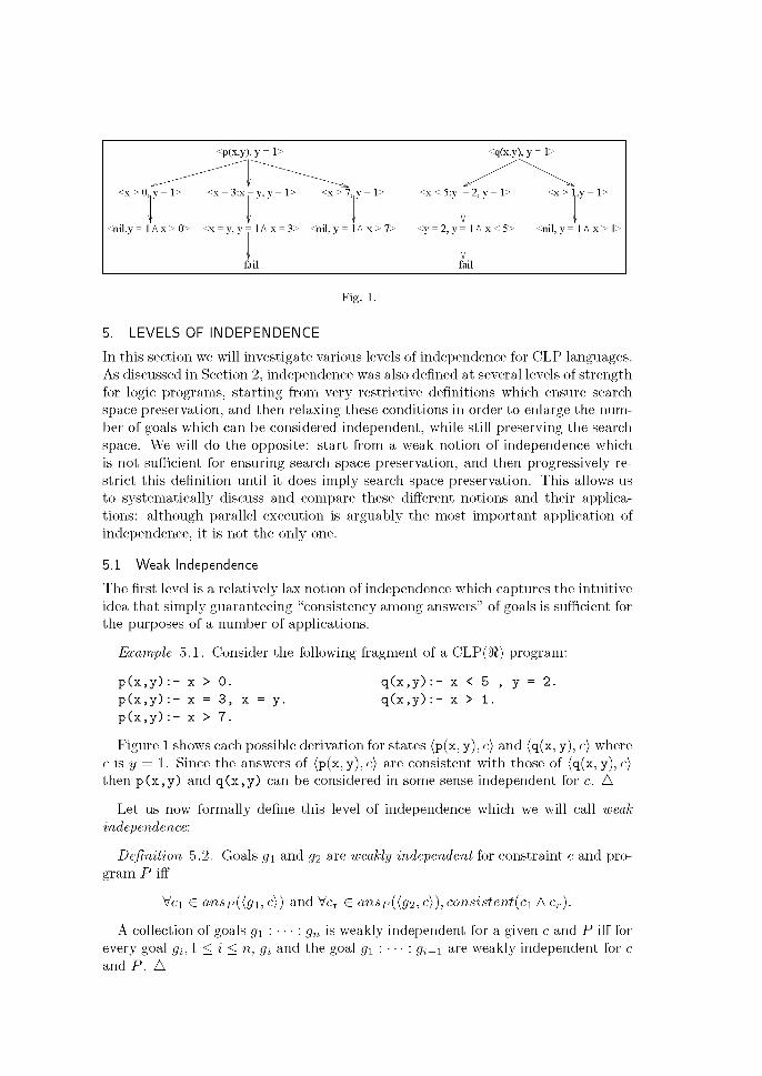
Fig. 1.

5. LEVELS OF INDEPENDENCE

In this section we will investigate various levels of independence for CLP languages. As discussed in Section 2, independence was also defined at several levels of strength for logic programs, starting from very restrictive definitions which ensure search space preservation, and then relaxing these conditions in order to enlarge the num­ber of goals which can be considered independent, while still preserving the search space. We will do the opposite: start from a weak notion of independence which is not sufficient for ensuring search space preservation, and then progressively re­strict this definition until it does imply search space preservation. This allows us to systematically discuss and compare these different notions and their applica­tions: although parallel execution is arguably the most important application of independence, it is not the only one.

5.1 Weak Independence

The first level is a relatively lax notion of independence which captures the intuitive idea that simply guaranteeing "consistency among answers" of goals is sufficient for the purposes of a number of applications.

Example 5.1. Consider the following fragment of a CLP(K) program:

p ( x , y ) : p ( x , y ) : p ( x , y ) :

- x > 0. - x = 3 , x - x > 7.

= y-q ( x , y ) : q ( x , y ) :

- x < 5 - x > 1.

y = 2.

Figure 1 shows each possible derivation for states (p(x, y), c) and (q(x, y), c) where c is y = 1. Since the answers of (p(x, y), c) are consistent with those of (q(x, y), c) then p(x,y) and q(x,y) can be considered in some sense independent for c. A

Let us now formally define this level of independence which we will call weak independence:

Definition 5.2. Goals g\ and #2 are weakly independent for constraint c and pro­gram P iff

Vci € ansp((g\, c}) and Vcr G ansp((g2, c)), consistent{c\ A c r).

A collection of goals g\ : • • • : gn is weakly independent for a given c and P iff for every goal gi, 1 < i < n, gi and the goal g\ : • • • : gi-\ are weakly independent for c and P. A

Note that , according to this definition, goals which fail (those for which the set of answers is empty) for a given constraint are weakly independent of all other goals. Also note tha t the appropriateness of the definition depends on the assumption tha t defnP renames local variables in ansp((gi,c)) and ansp({g2,c)) apart . Without this assumption, they would need to be existentially quantified.This is also t rue for subsequent definitions of independence.

Lemma 5.3. Goals g\ and #2 are weakly independent for constraint c and pro­gram P iff Vci G ansp({gi, c}), there exists a bijection which assigns to each node in a successful branch of treep({g2, c)) a corresponding node in a successful branch of treeP((g2,c1)). A

P R O O F . Let 7 be the local variable correcting renaming for treep((g2,c)) and treeP{{g2,ci)).

Let us first assume that , for each c\ G ansp({gi, c}), there exists a bijection which assigns to each node in a successful branch of t r e ep ((32, c)) a corresponding node in a successful branch of t r e e p ((32, c\)). Consider some answer c\ G ansp((gi, c)) and answer cr G ansp({g2, c)). Since cr is an answer, there is a success node r = {nil, cr) in treep({g2, c)). By assumption, there is a corresponding node s in t r e ep ((32, c\)). Prom Lemma 4.3, s = (nil,cs). From Lemma 4.4 we have tha t cs is equivalent to (ci A 7(c r ) ) . Since s is on a successful branch, cs is consistent. Thus 7(c s) is consistent. From Lemma 4.3, 7(01) = ci and 7 is its own inverse. Thus,

7(c s) = 7(01 A 7(c r ) ) = 7(01) A 7(7(0,.))) = ci A c r

and so consistent(c\ A c r) holds. Now consider the other direction. Let us assume tha t g\ and #2 are weakly inde­

pendent for c and P. By Lemma 4.8, for all nonfailure nodes, and in particular those in successful branches of t r e e p ((32, ci)) , there exists a corresponding node with the same pa th in a successful branch of treep ((32, c)). From the assumption of weak independence, for each node r = {Gr, cr) in a successful branch of treep((</2, c)) we have tha t consistent{c\ A c r) holds. And since

7(ci A c r) = 7(01) A 7(c r ) = ci A 7(c r )

we have tha t consistent(c\ Aj(cr)) must also hold. By Lemma 4.4, the consistency tests for obtaining the nodes with the same pa th as r are performed over a constraint cs satisfying cs <-> c\ A 7 (c r ) , and thus consistent(cs) must also hold. As a result, there exists a nonfailure node s in treep({g2, c\)) with the same pa th as r. And by Lemma 4.7 we have tha t s and r correspond. •

The usefulness of weak independence is based on the following result:

THEOREM 5.4. Let g\ : ••• : gn be a collection of weakly independent goals for constraint c and program P. Let gi,f < i < n be a goal such that there exists c\ G ansp({gi : • • • : <?j_i, c)) with ansp((gi,c\)) = 0. Then, for every c2 G ansp({gi : • • • : g j _ 1 ; c)), ansp{{gu c2)) = 0. A

P R O O F . By assumption, the collection of goals g\ : • • • : gi is weakly inde­pendent for c and P. By definition of weak independence, gi and the goal g\ : • • • : gi-\ are weakly independent for c and P. Also by assumption we have tha t there exists c\ G ansp({gi :••• : g j_ i , c ) ) with ansp({gi,ci)) = 0. This means

that there is no successful branch in ireep((<?$, ci)). By Lemma 5.3 we have that Vci G ansp({gi : • • • : gj_i,c}), there exists a bijection which assigns to each node in a successful branch of treep({gi,c)) a corresponding node in a success­ful branch of ireep((<?$, ci)). As a result, there can be no successful branches in treep((gi,c)). From the definition of the operational semantics, for every c2 G ansp({gi : • • • : <?j_i, c}) we have that c2 —> c. By completeness of consistent, there can be no successful branches in any treep({gi,c2)) such that c2 —> c. Thus, ansP((gi,c2)) = 0 . •

The above property is, in principle, useful for performing optimizations which are based on determination of producer-consumer relationships, such as intelli­gent backtracking. Backtracking occurs during exploration of the derivation tree whenever a failure node is reached. In the standard operational semantics, control "backtracks" to the closest ancestor with unexplored branches, thus ensuring depth-first exploration of the derivation tree. With intelligent backtracking [Bruynooghe and Pereira 1984], however, control may directly backtrack further up the tree. It requires analyzing, upon failure, the causes of the failure and determining the ap­propriate ancestor to backtrack to that can eliminate the failure while maintaining correctness, thus avoiding unnecessary computation.

A simple form of intelligent backtracking can be based on the notion of weak independence. Let g\ : • • • : gn be a set of goals which are weakly independent for the store c. Theorem 5.4 ensures that whenever there exists a goal g^ 1 < i < n for which no answers for goal gi are found, execution can safely backtrack to the choice-point placed just before gi, skipping all the choice-points in between.

It follows from the results in the previous section, that weak independence is not sufficient for ensuring search space preservation, since only successful derivations of the goals have been considered and the search space can also be affected through interactions with derivations failed or infinite derivations.

Example 5.5. Consider the previous example. Assume that we start from the state (p(x, y) : q(x, y),y = 1). It is clear that the search space associated with (q(x, y), y = 1 A x > 7} is smaller than that associated with (q(x, y), y = 1), since the derivation in which x < 5 appears would fail earlier—as soon as x < 5 is checked for consistency with the store. A

5.2 Strong Independence

We can define a more restrictive concept of independence, in the spirit suggested above, by taking into account all partial answers:

Definition 5.6. Goal g2 is strongly independent of goal g\ for constraint c and program P iff

Vci G ansp((g\, c}) and Vcr G pansp({g2, c)), consistent{c\ A cr)

A collection of goals g\ : • • • : gn is strongly independent for a given c and P iff for every g^ 1 < i < n, then gi is strongly independent of the goal g\ : • • • : gi-\ for c and P. A

Note that while weak independence is symmetric, strong independence is not.

Example 5.7. In the example given in Figure 1, p ( x , y ) is strongly independent of q (x ,y) for the constraint c = y = 1, since all answers to (q(x, y), c) are consistent with part ial answers of (p(x,y) ,c) . However, q ( x , y ) is not strongly independent of p ( x , y ) for the same constraint c. A

Also, note tha t if a goal #2 is strongly independent of another goal g\ for c, then g\ and §2 are weakly independent for c.

We will now prove some properties of strongly independent goals. The main result is tha t goal §2 is independent of g\ for a given constraint c if and only if the search space is preserved. Intuitively the following theorem states tha t consistency between the answers of {gi, c) and the partial answers of (#2, c) and (#2, c\) precludes pruning any branches, thus ensuring search space preservation. And vice-versa, search space preservation indicates no pruning and, thus, consistency.

THEOREM 5.8. Goal </2 is strongly independent of goal g\ for constraint c and program P iff

Vci G ansp((gi,c)), the search spaces of (<?2,c) and (g2, c\) are the same. A

P R O O F . Let 7 be the local variable correcting renaming for treep({g2,c)) and treeP{{g2,ci)).

Let us first assume tha t Vci G ansp({gi,c)) the search spaces of ((72, c) and (<?2,ci) are the same. By definition of search space, there exists a bijection which assigns to each node r in treep({g2,c)) a corresponding node s in treep({g2,ci)). By Lemma 4.7 each r and s are either both failure or both nonfailure nodes. For nonfailure nodes, say s = {Gs,cs) and r = ( G r , c r ) , by Lemma 4.4 we have tha t cs is consistent and equivalent to (c\ A 7 (c r ) ) . From properties of 7 it follows tha t consistent(ci Acr) must also hold. Since r refers to the nodes not only in successful but also in failure branches, it contains all partial answers and, thus, 32 is strongly independent of g\ for c and P.

The other direction uses a proof by contradiction. Let us assume tha t while 32 is strongly independent of g\ for c and P, the search spaces of (#2, c) and (#2, c\) are not the same. By Lemma 4.8, there must exist a node s = fail in treep({g2, c\)) obtained by applying —>cf and a node r = {Gr, cr) in treep({g2, c)) with the same pa th obtained by applying -^c such tha t their parents correspond. By construction, 7(01) = ci, and thus, by strong independence, consistent(c\ Aj(cr)) must also hold. By Lemma 4.4, the consistency test performed for obtaining s was applied to the constraint cs ^ c\A~f(cr). But, consistent(cs) holds, contradicting s being fail. •

This theorem ensures tha t strong independence is not only sufficient but also necessary for ensuring preservation of search space. Thus, from Theorems 4.9 and 4.10, correctness and efficiency of the parallel execution of a set of strongly indepen­dent goals for current constraint store c holds iff each goal is strongly independent for current constraint store c of the sequence composed of goals to its left.

Apart from parallelization, this theorem also provides a basis for goal reorder­ing, an important optimization for CLP languages. Marriott and Stuckey [1992] suggested reordering the goal cA g to g A c, where c is a primitive constraint, when­ever c and g are strongly independent for all possible constraint stores occurring before executing c and g. The motivation for this is tha t variables in c may become

uniquely defined by g, enabling the constraint c to be replaced by either an assign­ment statement or a simple Boolean test. If this is true, especially in the case g is recursive, large speedups are obtained. We can lift this idea to the level of goals and thus reorder goals as well.

It is difficult to give simple yet general conditions which ensure that the reordering of two goals reduces the search space. However, one simple condition that ensures that the reordering does not increase the search space is that the rightmost goal is "single solution" and strongly independent of the leftmost goal. Note that any deterministic goal, and in particular a primitive constraint, is single solution.

Definition 5.9. A goal g is single solution for constraint c and program P iff the state (g, c) has at most one successful derivation in P. A

THEOREM 5.10. If goal g2 is both strongly independent of goal g\ and single solution for constraint c and P then

cost({g2 : gi, c)) < cost{{gi : g2,c)). A

The proof comes directly from Lemma 4.8 and the given CLP operational se­mantics. Note that the search space can be decreased for two reasons. First, due to the asymmetry of strong independence g2 can decrease the search space of g\ for c. Second, the answer for g2 (if any) will not be recomputed when each answer to (7i is found.

5.3 Search Independence

As discussed in Section 2.2, in the independent and-parallel model, parallel goals are executed in different environments. The isolation of the environments quite ac­curately reflects the actual situation in distributed implementations of independent and-parallelism [Conery 1987]. However, in models designed for shared addressing space machines, such isolation of environments is not imposed by the machine archi­tecture and thus, in practice, the goals executing in parallel generally share a single binding environment (e.g., Hermenegildo and Greene [1990] and Lin [1988]). The amount of overhead introduced by requiring isolated environments (either copying the environment or renaming the goals, plus conjoining the solutions) in these ma­chines, suggests that such isolation should not be implemented unnecessarily. Fur­thermore, sharing the environments allows us to avoid performing the conjunction of the answers obtained from the parallel execution, since this happens automat­ically through the use of a shared constraint store. One might think that if we ensure that g2 is strongly independent of g\ with respect to a given constraint store c, then we can execute them in parallel in the same environment while preserving the correctness and efficiency with respect to the sequential execution of (g\ : g2,c). However, this is not true since, again, we have only considered the successful deriva­tions of g\ and, in this new context, it is possible for the execution of {g2, c) to prune the search space of {gi, c), which may lead to incorrect answers.

Example 5.11. Consider the following CLP(K) program:

p ( x ) : - x = 2, f a i l . q ( x ) : - x = 1. p ( x ) : - x = 1.

Clearly q(x) is strongly independent of p(x) for true. Now consider the parallel execution of (p(x) : q(x),£rwe) in an environment with a shared constraint store. If parallel reduction starts by rewriting p(x) with the first rule, and the constraint x = 2 is processed, then the store becomes x = 2. Now if q(x) is reduced and x=l is added to the store, failure will result and evaluation of q(x) will backtrack. As there is no other rule in the definition of q(x), evaluation will wrongly fail, without finding the answer. A

For this reason we define a symmetric notion of strong independence which en­sures that neither goal can interfere with the other.

Definition 5.12. Goals g\ and gi are search independent for constraint c and program P iff

Vci G pansp((g\, c}) and Vcr G pansp((g2, c)), consistent{c\ A cr).

A collection of goals g\ : • • • : gn is search independent for a given c and P iff for every gi, 1 < i < n: gi and any goal formed with goals from g\ : • • • : g^\ : g^\ : • • • : gn

a r e search independent for c and P. Also, a collection of goals is search independent for a set of constraints (interpreted as their disjunction) C and P iff they are search independent for each c g C and P. Finally, a collection of goals is simply search independent for P iff they are search independent for the set of all possible constraints and P. A

Then, in the same spirit as Theorem 5.8 we can conclude:

Corollary 5.13. Goals g\ and #2 are search independent for constraint c and program P iff

Vci G ansp({gi,c)), the search spaces of ((72, c) and (<?2,ci) are the same, and

Vcr G ansp({g2, c)), the search spaces of {gi, c) and {gi, cr) are the same. A

6. ENSURING INDEPENDENCE "A PRIORI"

While compile-time detection of independence can be based on the previous defini­tions themselves, practical run-time detection cannot. This is because independence has been defined in terms of the answers and partial answers produced by the goals, but, in practice, we are interested in an "a priori" detection of independence condi­tions (i.e., when detection must be performed just before executing the goals, and without actually having to execute them). In order to do this, (run-time) condi­tions for ensuring independence must be based only on information which is readily available before executing the goals, namely, the current constraint store and the variables appearing in the goals. One consequence is that an a priori test will not be able to distinguish between the various notions of independence—weak, strong, and search—introduced before.

Our first approach is to define conditions which must hold for each constraint defined over the variables of each goal:

Definition 6.1. Goals g\(x) and giiy) are projection independent for constraint c iff for all constraints c\ and C2, if consistent(cA 3_gci) and consistent(cA 3_^C2) hold then consistent^ A 3_gCi A 3_^C2) also holds. A collection of goals g\ :

• • • : gn is projection independent for a given c iff for every gi, 1 < i < n: gi and the goal g\ : • • • : g^\ : gi+i : • • • : gn are projection independent for c and P. Also, a collection of goals is projection independent for a set of constraints (interpreted as their disjunction) C iff they are projection independent for each c G C. Finally, a collection of goals is simply projection independent iff they are projection independent for the set of all possible constraints. A

Since the execution of a goal can only add constraints on local variables and the arguments of the goal, it is straightforward to prove the following result:

THEOREM 6.2. Goals g\ and gi are search independent for constraint c and any program P if they are projection independent for c. A

It follows tha t , since search independence implies strong independence, which in tu rn implies weak independence, projection independence also implies weak and strong independence.

Naive application of the definition of projection independence implies testing all possible consistent constraints over the variables of each goal. A more useful characterization of projection independence follows. It is based on identifying those variables which are "fixed" in a constraint c where a variable x is fixed in c if c implies tha t x has a single value. We let fixed(c) denote the set of fixed variables in c.

THEOREM 6.3. Goals g\(x) and gi{y) are projection independent for constraint c if

(x Pi y C ftxed(c)) and ( 3_ g c A 3_^c —> 3_yugc). A

P R O O F . Assume tha t the condition holds but there exist two constraints c\ and C2 such tha t both c A 3 _ g c i and cA3_^C2 are consistent but c A 3 _ g c i A3_^C2 is not. By assumption x n y C fixed(c), and therefore 3_ g c i A 3_^C2 must be consistent. Also by assumption, 3 _ g c A 3_^c implies 3_yU gc, and therefore 3_y U g cA 3_ g c i A 3_yC2 is consistent, which contradicts the assumption tha t c A 3_ g c i A 3_^C2 is inconsistent. •

This condition is not only sufficient but also necessary for projection indepen­dence whenever the constraint domain is sufficiently expressive, tha t is,

Definition 6.4. A constraint domain has nameahle elements if

• for any constraint c and variable x, if x is not fixed in c, then there exist primitive constraints of form x = l\ and x = h where l\ and l<i are variable-free expressions such tha t c A x = l\ and c A x = h are consistent but c A x = l\ A x = I2 is not consistent; and

• if ci 7^ C2, where c\ and C2 are conjunctions of possibly existentially quantified primitive constraints, then there exists a conjunction of primitive constraints, d, of form xi = li A • • • A X2 = h where the Xj are distinct variables and the U are variable-free expressions such tha t c\ A d is satisfiable but C2 A d is not. A

These conditions are satisfied by any constraint domain which has an expression (i.e., a "name") for each value in its domain which can be distinguished by the

6Note that ( 3 - J C A 3 - J C ^ - 3—yuxCj always holds.

primitive constraints. To the best of our knowledge, all constraint domains used in practice have nameable elements. As an example of a constraint domain without nameable elements, consider a restricted integer constraint domain where the only primitive constraint is equality and the only nonvariable expression is 0. Then a variable might not be fixed, but we still cannot find two values which satisfy the first condition above.

THEOREM 6.5. For constraint domains with nameable elements, goals g\(x) and 92 (y) are projection independent for constraint c only if

{x Pi y C fixed(cj) and ( 3_ g c A 3_^c —> 3_yugc). A

P R O O F . Let us reason by contradiction and assume tha t although g\ (x) and #2 (y) are projection independent for c, there exists z G xP\y such tha t z ^ fixed(c). Then, from the nameable element assumption there must exist variable-free expressions l\ and I2 such tha t cA {z = l\) and cA (z = h) are consistent but cA (z = h) A (z = 12) is not consistent. Therefore, c\ = (z = h) and C2 = (z = 12) do not satisfy the conditions required by projection independence, and there is a contradiction.

Now assume tha t (x n y C fixed(c)) but (3_ g c A 3_^c) -f-> 3-yUxc then, from the nameability assumption there must exist two sequences of variable-free expressions lx and ly such that (1) (3_ g c A 3_^c) A x = lx A y = ly is consistent but (2) (3_yU gc) Ax = lx Ay = ly is not consistent. It follows from (1) tha t both cAx = lx

and cAy = ly are consistent. Together with (2) this means that , c\ = (x' = lx) and C2 = (y' = ly) do not satisfy the conditions required by projection independence, and there is a contradiction. •

Intuitively, the above proof is based on the fact tha t the only way in which variables in x can affect the values of the variables y (and vice-versa), is by either (a) having nonfixed variables in common or (b) appearing together in some "relevant" constraint. The condition above specifically eliminates these two possibilities.

Example 6.6. Consider the goals g\{x,y),g2{z,w) and the constraint x + y + z + w = 7. It is obvious tha t the goals satisfy (a) but not (b) above, since the constraint x + y + z + w = 7is relevant for the relationship between the variables in {x, y} and the variables in {z, w}. But if we add the constraint x + y = 5, then the old constraint x + y + z + w = 7 becomes irrelevant (it can be substi tuted by z + w = 2) since there is no longer a relationship between the variables in {x, y} and the variables in {z, w}. A

Corollary 6.7. Goals gi(x) and (72(2/) are search independent for constraint c and any program P if x n y C fixed(c) and 3_ g c A 3_^c —> 3_yU gc. A

The proof comes directly from Theorems 6.2 and 6.3.

Example 6 .8. Consider the goals g\{y) and (72(2) and constraint c = y>x,z>x. Now 3_{y}C = e, 3_{Z}C = e, 3_{j,z}C = e. Therefore, from Corollary 6.7, we know tha t g\{y) and (72(2) are search independent for c. A

The following theorem provides the link with the sufficient conditions defined in Hermenegildo and Rossi [1995] (briefly summarized in Section 2.2) for logic programs.

THEOREM 6.9. In the context of term equations, two goals are projection inde­pendent for constraint c iff they are strictly independent for mgu(c). A

P R O O F . There is a natural bijection between solved form equations and (idem-potent) substitutions. If 9 is {x\ i—> t i , ...,xn i—> £„} we define cons(9) to be the solved form equation xi = ti A • • • Axn = tn.

It follows from the definition of strict independence tha t two goals gi{x) and 92 (y) are strictly independent for c iff the sets

{{x £ x\ fi{x = t) £ c'} U | J {vars(t)\(x = t) £ c'})

and

{{y £ y\ £{y = t) £ c'} U \J {vars(t)\(y = t) £ c'})

are disjoint, where c' is cons(mgu(c)). Straightforward, but tedious, case analy­sis shows tha t the sets are disjoint holds iff c' is projection independent. Since c is equivalent to c', it follows tha t the sets are disjoint iff c is projection indepen­dent. •

Thus projection independence is the natural generalization of strict independence to arbitrary constraint domains. As a consequence of the above theorem, for term equations there is no need to actually project the constraint store over any set of variables. However, when constraint domains other than Herbrand are involved, the cost of performing a precise projection may be too high. For example, projection over the linear arithmetic constraints has exponential complexity.

A pragmatic solution is to find if variables are "linked" through the primitive constraints in the constraint store. In fact we can do better by noticing tha t we can ignore variables tha t are constrained to take a unique value. Note tha t in the following we will t reat a constraint c as a syntactic object, rather than in terms of its logical meaning.

More formally, the relation linkc(x,y) holds for variables x and y if there is a primitive constraint c' in c such tha t {x,y} C vars(c') \ fixed(c). The relation linksc(x, y) is the transitive closure of linkc(x, y). We lift links to sets of variables by defining Linksc(x,y) iff 3x £ x and By £ y such tha t linksc(x,y).

THEOREM 6.10. Goals gi(x) and gi{y) are projection independent for constraint c if ->Linksc(x,y). A

Note tha t the above theorem does not depend on the syntactic representation we choose for c. In fact, if the solver keeps a "normal form" for the current constraints, we are bet ter off using the normal form rather than the original sequence of con­straints as this allows the definition to be simplified. More precisely, constraints c are in normal form if they have form

x\ = fi(y) Ax2= h{y) A ••• A x„ = fn(y) A c'

where the fi are function symbols of the underlying constraint domain, the Xj are distinct variables disjoint from the variables y and vars(c') C y. Associated with the normal form is an assignment tp to the eliminated variables, namely,

{x\ i—> fi(y), ...,xn i—> fn(y)}- It is straightforward to verify that Linksc(x,y) iff Linksc>{vars{tj){x)), vars(ip(y))).

The condition imposed by Theorem 6.10, although clearly sufficient, is some­what conservative. For instance, although the goals g\{y) and gi{z) are search independent for c = y > xAz > x, Linksc({y}, {z}) holds due to the transitive clo­sure performed when computing linksc(y, z). Thus, if projection may be efficiently performed for the particular constraint domain and solver, it is better to use the conditions in Theorem 6.3 to determine search independence at run time.

One important issue that remains to be discussed is the practical usefulness of the different independence notions. In the context of traditional logic programs, it has been shown [Bueno et al. 1999] that strict independence can be detected at compile-time with reasonable accuracy and can be proved at run-time without introducing great overheads. Non a priori notions are, however, a different issue since they cannot be used as the basis of run-time test and, thus, must be detected at compile-time. Unfortunately, even restricted non a priori notions, such as non-strict independence, are difficult to detect accurately at compile-time [Cabeza and Hermenegildo 1994]. This is not only because they require more complex analysis domains, but also because they require a particular analysis framework in which literals in the body of a clause are analyzed both in the context of the answers of previous literals and in isolation. In order not to exponentially increase the complexity, a possible approach would be to first perform a typical analysis, use that information to discard literals over which the desired optimization cannot be performed, and then reanalyze the rest in isolation.

In the case of other CLP languages, the problems found for non a priori indepen­dence notions become even more acute, due to the complexity of the domains needed to detect consistency of constraints accurately. In the case of a priori notions, pre­liminary experiments in Garcia de la Banda et al. [1996] show that traditional groundness and freeness information can be used to detect a priori independence at compile-time, but for accuracy, analysis domains specialised to the particular constraint domain used by the program, should be used. Regarding the compar­ison between the run-time test based on projection and link independence, the experimental evaluation showed two interesting conclusions. First, although there exist cases in which projection independence detects parallelism which link inde­pendence fails to detect, this is not a common case. Second, naive implementations of the independence tests introduce too much overhead, especially for projection independence.

7. SOLVER INDEPENDENCE

From the results in previous sections, it may be thought that search space inde­pendence is enough for ensuring not only the correctness but also the efficiency of any transformation applied to the search independent goals. Unfortunately, as mentioned in Section 5, this is not true in general.

Example 7.1. Consider the state (p(x) : q(x,y, z, w), true) and the program P:

p(x) <— x = 1. q(x,y ,z ,w) <— x + l = y , y = 2 + z , 2 * x + y = w , y > x , w > z .

It is easy to see that p(x) and q(x,y ,z ,w) are search space independent for true and P. However, executing (q(x, y, z, w), true) is more expensive than executing (q(x, y, z, w), x = 1). The reason is that while in the former case a relatively com­plex constraint solving algorithm (such as the Simplex introduced later) has to be applied, in the latter only simple value propagation is needed. As a result, the par-allelization or the reordering of the goals in the above state may actually produce a slowdown. A

The problem is that the amount of work performed when applying a particular transition rule is not always independent of the state to which this transition rule is applied. There are two different cases. On one hand, given a program P and a state s in which the leftmost literal is an atom a, the amount of work performed when applying the -^r or —>rf transition rules to s is identical to that performed when applying the same transition rule to state s' as long as the leftmost literal in the sequence of literals of s' is a variant of a, since the constraint stores in s and s' are not taken into account. On the other hand, given a program P and a state s in which the leftmost literal is a constraint c', the amount of work performed when applying the -^c and —>cf transition rules to s can be different to that performed when applying the same transition rule to state s' even if the leftmost literal in the sequence of literals of s' is a variant of c'. The key is in the differences between the constraint stores of s and s'.

Therefore, although as shown in the previous sections search space preservation ensures that for each transition rule the number of applications of this transition rule in the derivation trees of each state is preserved, it does not ensure the preservation of the amount of work when the -^c and —>cf transition rules are applied and the store in each state is different. The main problem is that the constraint solver is viewed as a black box, i.e., the operational semantics allow us to see the transitions applied at the higher level, but not those performed by the constraint solver at each of those high-level transitions. If we could have access to such "low-level" transitions, the amount of work performed by the constraint solver in adding a particular constraint to a particular store, would become explicit, and it could be characterized in terms of search space, analogously as for the high-level transitions. This is in fact the approach taken in Bueno et al. [1998].

Therefore, it is clear that modifying the order in which a sequence of primitive constraints is added to the store may have a critical influence on the time spent by the constraint solver algorithm in obtaining the answer, even if the resulting constraint is consistent. In fact, this issue is the core of the reordering transforma­tion described in Marriott and Stuckey [1992]. This variance in the cost of adding primitive constraints to the store has been ignored as a factor of negligible influ­ence in traditional logic programming. This is due to the specific characteristics of the standard unification algorithms [Paterson and Wegman 1978; Martelli and Montanari 1982]—we will return to this point later. However, as shown before, it cannot be ignored in the context of other CLP languages. For this reason, we now introduce the notion of constraint solver independence, a new type of independence which, although orthogonal to search space independence, is also needed in order to ensure the efficiency of transformations such as goal reordering and independent and-parallelization.

Intuitively, two sequences of primitive constraints are independent of each other for a given solver if adding them to the current constraint store in any "merging" has the same overall cost. We now make this idea more precise. Let Solv be a particular constraint solver and c and c' sequences of primitive constraints. We let scost(Solv, c, c') be the cost of adding the sequence c' to the solver Solv after c has been added. To illustrate the vagaries of constraint solving we note that even in "reasonable" constraint solvers such as, for example, that employed in CLP (3ft), we do not have that, if c" is a subsequence of c',

scost(Solv, c, c") < scost(Solv, c, c'),

as witness Example 7.1 above. We let merge(c, c') be the set of all mergings of the constraint sequences c and

d.

Definition 7.2. Constraint sequences c' and c" are K-independent for store c and solver Solv iff consistent(c' A c" A c) implies that for every c\, C2 G merge(c', c"), scost(Solv, c, c\) — scost(Solv, c, C2) < K. A

The intuition behind the parameterization of the definition is that the cost be bound by, for instance, a constant value or perhaps a linear function of the num­ber of shared variables among the sequences, where different levels of cost can be tolerated by different applications, also depending on the constraint system being used.

The obvious way to define independence for a solver is by ensuring that adding any pair of consistent sequences of constraints in any order leads to only small differences in cost. This is captured in the following definition.

Definition 7.3. A constraint solver Solv is independent iff for all constraint se­quences c, c' and c", c' and c" are K-independent for c and Solv, where K is a "small" constant value. A

Unfortunately, many reasonable constraint solvers do not satisfy solver indepen­dence. In many applications a weaker notion is acceptable, namely that the solver should be solver independent only for sequences which do not "interfere." This notion is inspired by the kind of constraints obtained from projection independent goals (or their almost equivalent characterization provided by Theorems 6.3 and 6.5).

Definition 7.4. A constraint solver Solv is projection independent iff for all con­straint sequences c, c', and c", if vars(c') n vars(c") C fixed(c) and 3-«arS(c ' )cA ^-vars{c")C - • ^-Vars{c')\jvars{c")C, then c' and c" are K-independent for c and Solv, where K is a "small" constant value. A

An even weaker notion of independence holds if we only consider constraints whose variables are not linked in any way through the store.

Definition 7.5. A constraint solver Solv is link independent iff for all constraint sequences c, c' and c", if -^Linksc(vars(c'),vars(c")) then c' and c" are solver K-independent for c and Solv, where K is a "small" constant value. A

In practice link independence seems more useful than projection independence: we claim that most reasonable constraint solvers are link independent and that,

therefore, the efficiency of many optimizations, such as and-parallelism, can be ensured once the adequate a priori notion is proved to hold for the goals involved in the optimization.

In order to exemplify the applicability of the previously defined notions we will review a few examples of solvers with respect to their solver independence charac­teristics.

In many CLP systems, for example CLP(K) and Prolog-Ill [Colmerauer 1990], constraint testing over systems of linear equations and inequations is performed using an incremental version of the simplex algorithm [Marriot and Stuckey 1998]. Essentially this involves incrementally recomputing a normal form for the constraint store when a new constraint is added. This is done by a succession of "pivots" which exchange the variables being eliminated. When a constraint is first encountered it is "simplified" by eliminating the variables from it. If this reduces the constraint to a simple assignment or Boolean test, then, for efficiency, the constraint is not passed to the constraint solver but is handled by the constraint solver "interface." In order to recognize such assignments or tests the solver keeps track of all variables which are constrained to a fixed value. For efficiency, the normal form "tableaux" is stored using a sparse matrix representation as a list of lists of nonzero entries. Let this constraint solver be called Simplex.

It is easy to construct examples showing that Simplex is neither independent nor projection independent. However, we do have that Simplex is link independent. This is because if the constraints in c' and c" are not linked through c, then their normal form in the tableaux does not share variables. Since the tableau is stored using a sparse representation, pivoting or eliminating a variable in an equation derived from c' will not consider equations derived from c", since they do not share nonzero entries in the tableau (and vice versa). If c' and c" share variables that have a fixed value then these variables will essentially be eliminated from the tableau and replaced by their value thus removing the connection between them.

We believe that the reason Simplex is link independent is typical of many solvers used in practice. It is instructive to reconsider unification algorithms as solvers for equality constraints over the domain of Herbrand terms and study their indepen­dence characteristics. It is clear that most reasonable unification algorithms would satisfy the conditions of projection independence, and in particular those which are "linear," i.e., which have the property of performing a number of atomic steps which is linear in the size of the terms being unified [Paterson and Wegman 1978; Martelli and Montanari 1982]. Furthermore, if we denote by LinUnif a unification algorithm belonging to the latter class, then we have that LinUnif is independent.

It is interesting to point out that independence does not hold even for all term equation solvers. For example, the cost of the original unification algorithm of Robinson [1965], which is exponential in the worst case, can vary by more than a constant factor depending on reordering. The algorithm used in most practical logic programming systems is actually an adaptation of Robinson's. However, these algorithms can actually be linear because either they (incorrectly) do not perform the occur check, and because they do not materialize the substitutions, but rather keep them in an implicit representation using pointers). In fact, in most practical implementations the difference of execution time after reordering will actually be very close to zero. This is the assumption that is used in practice in optimizations

of logic programs based on independence, and it is this assumption which makes the classical view of expressing independence in logic programs only in terms of search independence correct.

8. ALLOWING DYNAMIC SCHEDULING

In previous sections we have studied independence for languages in which calls are evaluated using a fixed left-to-right scheduling strategy. Thus, our results do not directly apply to many modern CLP languages, since these often provide a form of coroutining called dynamic scheduling. That is, in these languages the default scheduling is still left-to-right, but some calls may be dynamically "delayed" until their arguments are sufficiently instantiated.

We now extend our independence results to dynamically scheduled languages. This is important for at least four reasons. First, as we have suggested many existing CLP languages already provide flexible scheduling. Therefore, in order to be practical, independence-based optimizations must handle dynamically scheduled programs. Second, dynamic scheduling has a significant cost, increasing the need of applications which improve efficiency. Third, dynamically scheduled languages are considered as promising target languages for the implementation of concurrent constraint logic languages [Debray 1993; Saraswat 1987; Ueda and Chikiyama 1985]. Fourth, dynamic scheduling is also present in some logic programming languages but has been ignored in work on parallelization of logic programs.

8.1 Operational Semantics

The operational semantics of CLP programs with dynamic scheduling is slightly more complex than that given earlier for CLP languages with fixed left-to-right literal scheduling. Again the semantics may be presented as a transition system on states. However, a nonfail state (G, c, D) now also contains a sequence of delayed atoms, D. The other components—the sequence of nonexecuted literals, G, and the constraint store, c—remain the same. In addition to the constraint solving function consistent(c), the operational semantics is parameterized by the predicate delay(a, c), which holds iff a call to atom a delays with the constraint c, and the function woken(D, c) which returns the sequence of atoms in D which are woken for constraint c. Note that the order of the atoms returned by woken is system dependent. Furthermore, the parametric functions delay and woken are assumed to satisfy the following five conditions:

• If G = woken(D, c), then a G G i f f a G - D A —tdelayia, c).

• If G\ = woken(Di,c) and G<i = woken(D2,c), D\ is a subsequence of D<i and for all a G D\ \ D2, delay (a, c) holds, then G\ = G<i-

• Let p be a renaming, then delay(a, c) iff delay(p(a), p(c)).

• del ay (a, c) iff del ay (a, 3_ tJars(a)c).

• If c —> c' and del ay (a, c), then delay (a, c').

The first condition ensures that there is a congruence between the conditions for delaying an atom and waking it. The second condition ensures that the order of woken goals only depends on their relative ordering in the sequence of delayed goals. The remaining conditions ensure that delay behaves reasonably, i.e., it does

not take variable names into account, is only concerned with the effect of c on the variables in a, and if an atom is not delayed, adding more constraints never causes it to delay

Let a denote an atom and c' a constraint. The transition rules are

a : G,c, D) ^d (G, c,a:D) if delay (a, c) holds;

a : G,c, D) -^r (B :: G, c, D) if delay (a, c) does not hold and B G defnP(a);

a : G,c, D) —>rf fail if delay (a, c) does not hold and defnP(a) = 0;

G, c, D) —>w (G' :: G,c,D\ G') where G' = woken(D, c), and G' is not empty

note that \ is assumed to preserve the relative order of the unwoken goals);

c' : G, c, D) -^c (G, c A c', D) if consistent(c A c') holds;

c' : G, c, D) —>cf fail if consistent(c A c') does not hold.

The above operational semantics extends that given earlier for traditional CLP languages by adding the —>,j and —>w transitions. Note that the conditions for applying each of the transition rules are still pairwise exclusive, except for —>w. We will assume that this transition rule has preference over the rest of the rules, thus being applied to any state (G, c, D) in which woken(D, c) is nonempty. The same result could also be achieved by combining the -^c and -^w transition rules, but given our interest in the particular characteristics of —>w, we have kept them separate. As before, we will assume a depth-first search strategy. All notions related to derivations and derivation trees are straightforward extensions of those defined for the CLP context. One difference is that answers may now contain a sequence of delayed goals and so consist of tuples whose first element is the answer constraint and whose second element is the delayed goal sequence.

We now generalize our earlier results to CLP languages with dynamic scheduling. We do this in two stages. First we assume that the initial sequence of delayed goals is empty. In the second stage we shall drop this assumption.

8.2 Independence When the Initial Sequence D is Empty

We start by extending our and-parallel execution model to this new context. As­sume that given the program P and the state (g\ : §2 : G, c, nil), we want to execute <?i and §2 in parallel. Then the execution scheme is the following:

• execute (gi, c, nil) and (#2, c, nil) in parallel (in different environments) obtaining the answers (c\,D\) and {cr,Dr) respectively,

• obtain cs = c\ A cr, and

• execute {G,cs,Dr :: D\).

Modulo the extra transformation rules, the definition of search space preservation remain the same as that given earlier. The definition of correctness is extended as follows:

Definition 8.1. Let s be the state {g\ : §2 '• G, c,nil) and P a program. The par­allel execution of g\ and §2 is correct iff for every (ci, D\) G ansp((gi, c, nil)) there exists a renaming 7 such that j(s) = s and a bijection which assigns to each answer {cs,Ds) G ansp((g2, c\, -Di)), an answer (ct, Dt) G ansp((nil,ci Ac r , Dr :: D\)) such that Ds = ^(Dt) and cs = 7(c t), where (cr, Dr) G ansp({g2, c,nil)). A

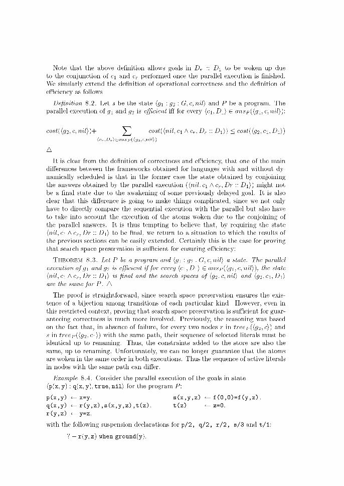
Note tha t the above definition allows goals in Dr :: D\ to be woken up due to the conjunction of c\ and cr performed once the parallel execution is finished. We similarly extend the definition of operational correctness and the definition of efficiency as follows

Definition 8.2. Let s be the s tate (g\ : </2 : G,c,nil) and P be a program. The parallel execution of g\ and #2 is efficient iff for every (c\, D\) G ansp((g\, c, nil)):

cost((g2,c,nil))+ 2 , cost((nil,c\ A cr, Dr :: D\)) < cost((g2,c\, D\)) {cr :Dr) £ansp ({32 :c:nil))

A

It is clear from the definition of correctness and efficiency tha t one of the main differences between the frameworks obtained for languages with and without dy­namically scheduled is tha t in the former case the state obtained by conjoining the answers obtained by the parallel execution ((nil, c\ A cr, Dr :: D\)) might not be a final s tate due to the awakening of some previously delayed goal. It is also clear tha t this difference is going to make things complicated, since we not only have to directly compare the sequential execution with the parallel but also have to take into account the execution of the atoms woken due to the conjoining of the parallel answers. It is thus tempting to believe that , by requiring the s tate (nil, c\ A cr, Dr :: D\) to be final, we return to a situation to which the results of the previous sections can be easily extended. Certainly this is the case for proving tha t search space preservation is sufficient for ensuring efficiency:

THEOREM 8.3. Let P he a program and (g\ : gi : G, c,nil) a state. The parallel execution of gi and g^ is efficient if for every (c\,D\) G ansp((g\,c,nil)), the state (nil, c\ A cr, Dr :: D\) is final and the search spaces of (gi, c, nil) and (gi, c\, D\) are the same for P. A

The proof is straightforward, since search space preservation ensures the exis­tence of a bijection among transitions of each particular kind. However, even in this restricted context, proving tha t search space preservation is sufficient for guar­anteeing correctness is much more involved. Previously, the reasoning was based on the fact that , in absence of failure, for every two nodes r in treep((g2,c)) and s in treep((g2,c\)) with the same path, their sequence of selected literals must be identical up to renaming. Thus, the constraints added to the store are also the same, up to renaming. Unfortunately, we can no longer guarantee tha t the atoms are woken in the same order in both executions. Thus the sequence of active literals in nodes with the same pa th can differ.

Example 8.4. Consider the parallel execution of the goals in s tate (p(x, y) : q(x, y), t rue , n i l ) for the program P:

p ( x , y ) <- x=y. s ( x , y , z ) <- f ( 0 , 0 ) = f ( y , z ) . q ( x , y ) <— r ( y , z ) , s ( x , y , z ) , t ( z ) . t ( z ) <— z=0. r ( y , z ) <- y=z.

with the following suspension declarations for p / 2 , q / 2 , r / 2 , s / 3 and t / 1 :

? — r(y, z) when ground(y).

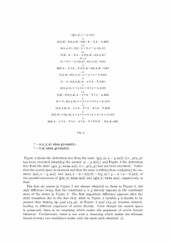
(q(x, y),x = y,nil> | r

(r(y, z) : s(x, y, z) : t(z) : x = 0, x = y, n i l )

Id (s(x, y, z) : t(z) : x = 0, x = y, r(y, z)>

Id (t(z) : x = 0, x = y, r(y, z) : s(x, y, z)>

a:e | d

(x = 0, x = y, r(y, z) : s(x, y, z) : t(z)>

(ni l , x = y A x = 0, r(y, z) : s(x, y, z) : t (z)) X-UJ

( r (y , z) : s(x, y, z) :, x = y A x = 0, t (z)>

| r (y = z : s(x, y, z) , x = y A x = 0, t (z)>

Xc (s(x, y, z) , x = y A x = 0 A y = z, t ( z ) )

X-UJ

(t(z) : s(x, y, z), x = y A x = 0 A y = z, n i l )

Ir

(z = 0 : s(x, y, z) , x = y A x = 0 A y = z, n i l )

(s(x, y, z ) , x = y A x = 0 A y = z A z = 0, n i l )

Ir (f(0, 0) = f(y, z) ,x = y A x = 0 A y = z A z = 0 ,n i l )

Xc {nil, x = y A x = 0 A y = z A z = 0 A f (0, 0) = f(y, z ) , n i l )

Fig. 2.

? — s(x, y, z) when ground(x). ? — t(z) when ground(z).

Figure 2 shows the derivation tree from the state (q(x,y),x = y ,ni l ) (i.e., p(x,y) has been executed obtaining the answer (x = y, ni l)) and Figure 3 the derivation tree from the state (q(x, y), true, nil) (i.e., p(x,y) has not been executed). Notice that the search space is identical and that the state resulting from conjoining the an­swers (nil, x = y, n i l ) and (nil, x = 0 A f (0, 0) = f (y, z) A y = z A z = 0, ni l ) of the parallel execution of (p(x, y), true, nil) and (q(x, y), true, ni l) , respectively, is final.

The first six states in Figure 2 are almost identical to those in Figure 3, the only difference being that the constraint x = y already appears in the constraint store of the states in Figure 2. The first important difference appears after the sixth transition due to the fact that, while in Figure 2 variable y is known to be ground thus waking up goal r ( y , z ) , in Figure 3 goal r (y , z ) remains delayed, leading to different sequences of active literals. Even though the search space is preserved, there is no renaming which makes the sequences of active literals identical. Furthermore, there is not even a renaming which makes the leftmost literal of every two nonfailure nodes with the same path identical. A

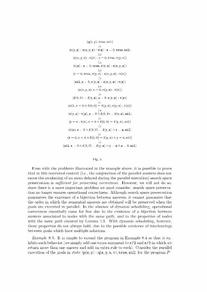
(q(x, y), true, nil)

|r

(r(y, z) : s(x, y, z) : t(z) : x = 0, true, nil)

Id (s(x, y, z) : t(z) : x = 0, true, r(y, z))

Id (t(z) : x = 0, true, r(y, z) : s(x, y, z))

Id (x = 0, true, r(y, z) : s(x, y, z) : t(z))

(nil, x = 0, r(y, z) : s(x, y, z) : t(z))

(s(x, y, z), x = 0, r(y, z) : t(z)>

|r

(f (0, 0) = f (y, z), x = 0, r(y, z) : t(z)>

(nil, x = 0 A f (0, 0) = f (y, z), r(y, z) : t(z)>

X-UJ

(r(y, z) : t(z),x = 0 Af(0,0) = f(y, z),nil)

Ir (y = z : t(z),x = 0 Af(0,0) = f(y, z),nil)

Xc (t(z), x = 0 A f (0, 0) = f (y, z) A y = z, nil)

Ir (z = 0, x = 0 A f (0, 0) = f (y, z) A y = z, nil)

Xc (nil, x = 0 A f (0, 0) = f (y, z)Ay = z A z = 0, nil)

Fig. 3.

Even with the problems illustrated in the example above, it is possible to prove that in this restricted context (i.e., the conjunction of the parallel answers does not cause the awakening of an atom delayed during the parallel execution) search space preservation is sufficient for preserving correctness. However, we will not do so, since there is a more important problem we must consider: search space preserva­tion no longer ensures operational correctness. Although search space preservation guarantees the existence of a bijection between answers, it cannot guarantee that the order in which the sequential answers are obtained will be preserved when the goals are executed in parallel. In the absence of dynamic scheduling, operational correctness essentially came for free due to the existence of a bijection between answers associated to nodes with the same path, and to the properties of nodes with the same path ensured by Lemma 4.3. With dynamic scheduling, however, those properties do not always hold, due to the possible existence of interleavings between goals which have multiple solutions.

Example 8.5. It is simple to extend the program in Example 8.4 so that it ex­hibits such behavior (we simply add one extra argument to r / 2 and s/3 in which we return more than one answer and add an extra rule to each). Consider the parallel execution of the goals in state (p(x, y) : q(x, y, u, v), true, nil) for the program P:

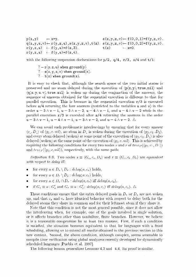
p ( x , y ) <- x=y. s ( x , y , z , v ) < - f ( 0 , 0 , l ) = f ( y , z , v ) . q(x,y ,u ,v)<— r ( y , z , u ) , s ( x , y , z , v ) , t ( z ) . s ( x , y ,z,v)<— f ( 0 , 0 , 2 ) =f ( y , z , v ) . r ( y , z , u ) <— f ( y , u ) = f ( z , 3 ) . t ( z ) <— z=0. r ( y , z , u ) <- f ( y , u ) = f ( z , 4 ) .

with the following suspension declarations for p / 2 , q / 4 , r / 3 , s / 4 and t / 1 :

? — r(y, z, u) when ground(y). ? — s(x, y, z, v) when ground(x). ? — t ( z ) when ground(z).

It is easy to check that , although the search space of the two initial states is preserved and no atom delayed during the execution of (p(x,y), t rue , n i l ) and (q(x, y,u, v), t rue , n i l ) is woken up during the conjunction of the answers, the sequence of answers obtained for the sequential execution is different to tha t for parallel execution. This is because in the sequential execution r / 3 is executed before s / 4 returning the four answers (restricted to the variables u and v) in the order u = 3 A v = 1, u = 3 A v = 2, u = 4 A v = 1, and u = 4 A v = 2 while in the parallel execution r / 3 is executed after s / 4 returning the answers in the order u = 3 A v = 1, u = 4 A v = 1, u = 3 A v = 2, and u = 4 A v = 2. A

We can avoid such problematic interleavings by ensuring tha t for every answer (ci, D\) of (<;i, c, nil), no a tom in D\ is woken during the execution of (#2, c\, D\), and every a tom delayed (woken) at some point of the execution of (#2, c\,D\) is also delayed (woken) at the same point of the execution of (#2, c, nil). This is achieved by requiring the following conditions for every two nodes s and r of treep({§2, ci,D\)) and treep((g2, c, nil)), respectively, with the same path:

Definition 8.6. Two nodes s = (Os,cs,Ds) and r = (Or,cr, Dr) are equivalent with respect to delay iff:

• for every a G Ds\ Dr : del ay (a, cs) holds,

• for every a G Dr \ Ds : del ay (a, cr) holds,

• for every a G Ds l~l Dr : del ay (a, cr) iff del ay (a, c s),

• if Gs = a : G's and Gr = a : G'r: del ay (a, cr) iff delay (a, c s) . A

These conditions ensure tha t the extra delayed goals in Dr or Ds are not woken up, and tha t cs and cr have identical behavior with respect to delay both for the delayed atoms they share in common and for their leftmost a tom if they share it.

Note tha t this condition is not the most general possible, since it does not allow the interleaving when, for example, one of the goals involved is single solution, or it affects branches other than nonfailure, finite branches. However, we believe it is a reasonable compromise for at least two reasons. First, if such a condition is satisfied, the situation becomes equivalent to tha t for languages with a fixed scheduling, allowing us to extend all results obtained in the previous section to this new context. Second, the above condition, although complex, seems amenable to compile-time verification using global analyzers recently developed for dynamically scheduled languages [Puebla et al. 1997].

The following lemma generalizes Lemmas 4.3 and 4.4. Its proof is similar.

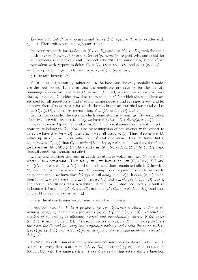
Lemma 8.7. Let P be a program and {g2, ci , -Di), ((72, c, ni/) be two states with c\ —> c. There exists a renaming 7 such that :

—for every two nonfailure nodes s = {Gs, cs, Ds) and r = (Gr, cr,Dr) with the same pa th in treep({g2,ci,Di)) and -f(treep({g2,c,nil))), respectively, such tha t for all ancestors s' and r' of s and r respectively with the same path, s' and r' are equivalent with respect to delay, Gs = Gr, Ds = Dr :: D\, and cs <-> [c\ A c r ) ;

—7((s ,2,ci,-Di}) = {g2,c1,D1) and j((g2,c,nil)) = (g2,c,nil);

—7 is its own inverse. A

P R O O F . Let us reason by induction. In the base case the only nonfailure nodes are the root nodes. It is clear tha t the conditions are satisfied for the identity renaming 7 since we have tha t D\ = nil : D\ and, since c\ —> c, we also have tha t c\ ^ ct\c\. Consider now tha t there exists a 7 ' for which the conditions are satisfied for all ancestors s' and r' of nonfailure nodes s and r, respectively, and let us prove there also exists a 7 for which the conditions are satisfied for s and r. Let r' = (G'r, c'r, D'r). Then, by assumption, s' = (G'r, c\ A c'r, D'r :: D\).

Let us first consider the case in which some atom is woken up. By assumption of equivalence with respect to delay we have tha t VaG D\. delay{a, c\ A c'r) holds. Thus, no a tom in D\ will be awoken in s'. Therefore, if some atom is woken up the a tom must belong to D'r. Now, also by assumption of equivalence with respect to delay we have tha t Va G D'r: delay (a, c\ Ac'r) iff delay (a, c'r). Thus, if some a G D'r

wakes up in r', it will also wake up in s' and vice-versa. Thus we have tha t if Ga = woken(D'r, c'r) then Ga = woken(D'r :: Di, c\ Ac'r). It follows that , for 7 ' = 7 we have r = (Ga : G'r,c'r,D'r \ Ga) and s = (Ga : G'r, cx A c'r, {D'r \ Ga) :: Dt), and thus all conditions remain satisfied.

Let us now consider the case in which no atom is woken up. Let G'r = c' : Gr

where c' is a constraint. Then for 7 ' = 7 we have tha t r = (Gr, c' A c'r, D'r) and s = (Gr, c\ A c' A c'r, D'r :: Di), and thus all conditions remain satisfied. Otherwise, G'r = a : Gr where a is an atom. By assumption of equivalence with respect to delay of r' and s' we have tha t delay(a, c'r) iff delay(a, c\Ac'r). If delay(a, c'r) holds, then for 7 ' = 7 we have tha t r = (Gr, c'r, a : D'r) and s = {Gr, c\ A c'r, a : D'r :: Di), and thus all conditions remain satisfied. If delay(a, c'r) does not hold 7 is built as in Lemma 4.3 and r = (B : Gr, c'r, D'r) and s = (B : Gr, c\ A c'r, D'r :: D-\), and thus all conditions remain satisfied. •

Given the above lemma we can now ensure the following:

THEOREM 8.8. Let P be a program, (g\ : g2 :G,c,nil) a state, and 7 a re­naming satisfying Lemma 8.7 for states (<?2jCi,-Di) and {g2,c,nil). Parallel ex­ecution of g\ and g2 is efficient, correct and operationally correct if for every (c\,D\) G ansp((g\,c,nil)), the search spaces of{g2,c,nil) and (g2,ci,Di) are the same for P, and for every two nonfailure nodes s and r with the same path in treep({g2, c\, D\)) and j(treep((g2,c,nil))), s and r are equivalent with respect to delay. A

P R O O F . By definition of search space preservation, there exists a bijection which assigns to every final state r = {Gr,cr,Dr) in treep({g2,c)) a final s tate s = {Gs,cs,Ds) with the same pa th in -f(treep({g2,ci))), thus establishing a bijection

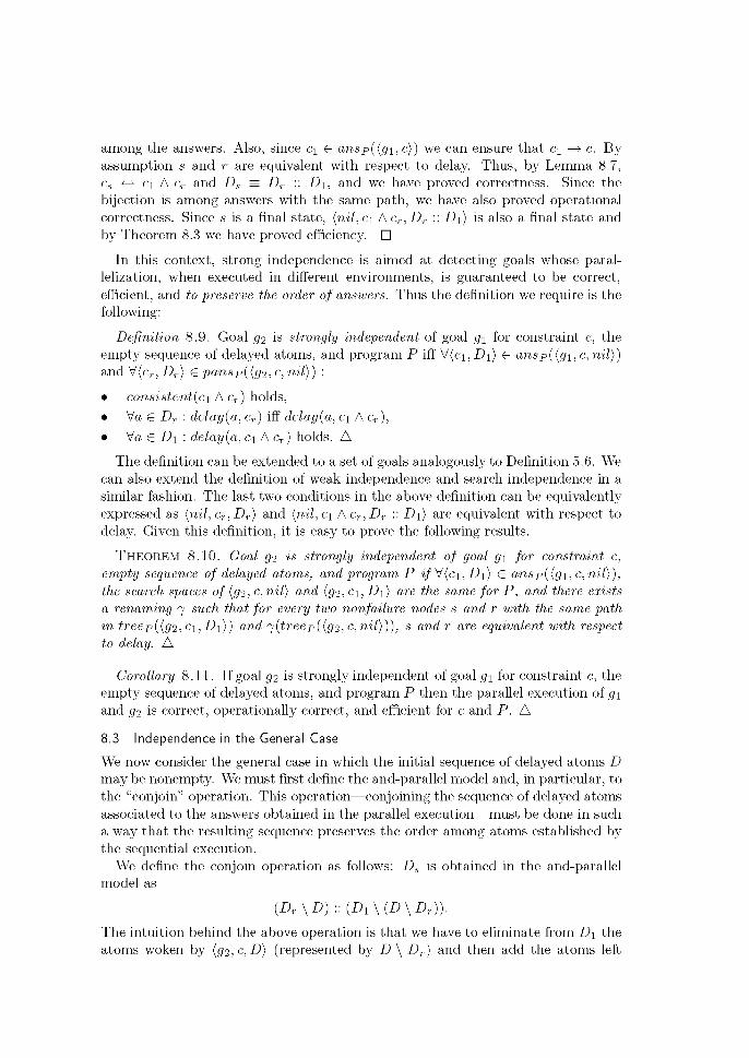
among the answers. Also, since c\ G ansp({gi, c)) we can ensure tha t c\ —> c. By assumption s and r are equivalent with respect to delay. Thus, by Lemma 8.7, cs ^ ci A cr and Ds = Dr :: D\, and we have proved correctness. Since the bijection is among answers with the same path , we have also proved operational correctness. Since s is a final state, {nil, c\ A cr, Dr :: D\) is also a final s tate and by Theorem 8.3 we have proved efficiency. •

In this context, strong independence is aimed at detecting goals whose paral-lelization, when executed in different environments, is guaranteed to be correct, efficient, and to preserve the order of answers. Thus the definition we require is the following:

Definition 8.9. Goal gi is strongly independent of goal g\ for constraint c, the empty sequence of delayed atoms, and program P iff V(ci, D\) G ansp({gi, c, nil)) andV(c r ,_D r) G pans p({g2,c, nil)) :

• consistent{c\ A cr) holds,

• Va G Dr : del ay (a, cr) iff delay (a, c\ A cr),

• Va G D\ : delay(a, c\ A cr) holds. A

The definition can be extended to a set of goals analogously to Definition 5.6. We can also extend the definition of weak independence and search independence in a similar fashion. The last two conditions in the above definition can be equivalently expressed as (nil, cr, Dr) and {nil, c\ A cr, Dr :: D\) are equivalent with respect to delay. Given this definition, it is easy to prove the following results.

THEOREM 8.10. Goal gi is strongly independent of goal g\ for constraint c, empty sequence of delayed atoms, and program P ify(ci,D\) G ansp((gi, c,nil)), the search spaces of (g2, c, nil) and (g2, c\, D\) are the same for P, and there exists a renaming 7 such that for every two nonfailure nodes s and r with the same path in treep((g2, c\, D\)) and ^{treep((<?2, c, nil))), s and r are equivalent with respect to delay. A

Corollary 8 .11 . If goal 32 is strongly independent of goal g\ for constraint c, the empty sequence of delayed atoms, and program P then the parallel execution of g\ and 32 is correct, operationally correct, and efficient for c and P. A

8.3 Independence in the General Case

We now consider the general case in which the initial sequence of delayed atoms D may be nonempty. We must first define the and-parallel model and, in particular, to the "conjoin" operation. This operation—conjoining the sequence of delayed atoms associated to the answers obtained in the parallel execution—must be done in such a way tha t the resulting sequence preserves the order among atoms established by the sequential execution.

We define the conjoin operation as follows: Ds is obtained in the and-parallel model as

(Dr\D)::(D1\(D\Dr)).

The intuition behind the above operation is tha t we have to eliminate from D\ the atoms woken by (g2,c,D) (represented by D\Dr) and then add the atoms left

delayed by (#2, c, D) which do not belong to the initial sequence (represented by (Dr\D)).

With this definition, the results obtained in the previous sections regarding the characteristics of both search space preservation and strong independence can be extended to this new context in a straightforward way.

8.4 Ensuring Independence "A Priori"

As mentioned earlier, it is important to find "a priori" conditions which ensure in­dependence. In this section we extend the earlier notion of projection independence to the broader context of languages with dynamic scheduling. Consider two goals <?i and #2 which are projection independent for constraint c. If the sequence of de­layed atoms D is empty, then we can ensure tha t the goals are search independent by simply detecting tha t the above condition holds. The intuition behind this fact is tha t if there are no delayed atoms before the execution of the goals, and they cannot affect the domain of each other 's variables, then their partial answers will be consistent and the instantiation state of their variables will not change no mat ter whether one is executed before or after the other, thus not affecting the atoms left delayed by the other goal. Formally, this is s ta ted as follows:

THEOREM 8.12. Goal gi is search independent of goal g\ for 'program P, con­straint store c, and empty sequence of delayed atoms D if the goals are projection independent for P and c. A

Of course search independence still implies weak and strong independence. A difference with respect to the previous cases does arise, however, when the

initial sequence of delayed atoms D is not empty. In this case the sufficient condition must take into account the constraints established on the variables which appear in the delayed atoms. The reason is tha t atoms woken during the execution of either gi(x) or 32(y) may introduce new constraints involving variables in bo th x and y.

The solution proposed is to ensure tha t D can be parti t ioned into two sequences in such a way tha t if we associate them to g\(x) and giiy) respectively, the two new goals are projection independent for the given c. While the first sequence corresponds to the delayed literals tha t depend on gi(x), the second one corresponds to those tha t depend on #2 (y) • If there exist delayed atoms which depend on neither gi(x) nor 32(y), they can be concatenated to either of the two sequences.

Definition 8 .13. Goals g\ and gi are projection independent for constraint c and sequence of delayed atoms D iff D can be parti t ioned into two sequences D\ and £>2 such tha t the goals g\ : D\ and #2 : P>2 are projection independent for c. A

THEOREM 8.14. Goal gi is search independent of goals g\ for constraint c and sequence of delayed atoms D if the goals are projection independent for c and D. A

The proof follows directly from Theorem 8.12. Again, search independence also implies weak and strong independence.

9. CONCLUSIONS AND FUTURE WORK

We have shown how a simple extrapolation of the logic programming-based defini­tions of independence to CLP turns out to be both not general enough in some cases

and erroneous in others, and identified the need in CLP for defining concepts of independence both at the search level and at the solver level. Several such concepts have been presented and shown to be relevant to several classes of applications. We have also proposed sufficient conditions for the concepts of independence proposed, which are easier to detect at run-time than the original definitions. Finally, we have extended our results to deal with CLP languages with dynamic scheduling.

Our results also provide insight into the theory of independence for logic pro­grams. The concepts proposed, when restricted to conventional logic programming, are equivalent to the traditional notions. They make explicit hidden assumptions related to properties of the standard unification algorithm and clarify the relation­ships between independence and search space preservation.

It is our belief that using the concepts of independence presented the range of applications of independence-related optimizations can be even larger in CLP than in logic programming.

One clear topic for future work is to develop analyses for determining indepen­dence at compile-time. One step in this direction is the analysis based on the LSign domain defined in Marriott and Stuckey [1994]. In this case the most straightfor­ward approach is to apply the definitions directly—the fact that the definitions are in terms of the run-time answer constraints is not so much of a problem, since the problem of predicting the state of the store after the execution of the goals is probably no more difficult than determining its state before such execution.

Another clear topic for future work is to apply the results to practical optimiza­tion tools for CLP languages. First, we are in the process of developing automatic parallelization tools based on these ideas. It appears feasible to extend the for­mal techniques that have been developed for this purpose in the context of logic programming, by using the herein proposed notions of independence [Bueno et al. 1999]. And, although the topic certainly requires more study, preliminary experi­ments confirm that useful speedups can be obtained automatically in practice by parallelizing independent goals [Garcia de la Banda et al. 1996]. Also, it appears possible to exploit more fine-grained forms of and-parallelism, provided the def­inition of independence is applied at the appropriate level: for example, stream and-parallelism can be exploited in CLP programs by considering the indepen­dence notions at the level of individual constraints rather than goals [Bueno et al. 1998].

Second, we have developed tools for reordering-based program optimization in the context of CLP languages without dynamic scheduling [Kelly et al. 1996]. However, reordering is even more interesting for the case of dynamic scheduling because the process of delaying a goal involves run-time overhead. Actually, dynamic scheduling can be seen as a run-time form of goal reordering, while the reordering optimization moves the position of goals at compile-time. The topic of reordering in the context of dynamic scheduling, in which independence can also be instrumental, is dealt with in more detail in Puebla et al. [1997].

Finally, our results can be used to detect "stability" [Janson and Haridi 1991]. This notion is used in the Andorra family of languages in general, and in the AKL language in particular, as the rule for control of one of the basic operations of the language—global forking. This operation amounts to starting and-parallel execu­tion of a goal which is nondeterministic. Stability for a goal is defined informally

as being in a state in which other goals running in parallel with it will not affect its execution. This is of course an undecidable notion, and in practice sufficient conditions are used in actual implementations. In particular, in the first implemen­tation of AKL, restricted to the Herbrand domain, the stability condition used is actually the classical notion of strict independence for logic programming [Pranzen 1992]. Since the AKL language is defined to be a constraint language, the notion of stability has to be generalized to the constraint level. As we have shown, general­ization cannot be done by directly applying naive liftings of the logic programming concepts of independence. We believe that the results presented in this paper will be of direct application.

ACKNOWLEDGMENTS

We thank Francisco Bueno, Lee Naish, and anonymous reviewers of previous ver­sions of this paper for their comments.

REFERENCES

A P T , K. 1990. Introduction to Logic Programming. In Handbook of Theoretical Computer Science, J. van Leeuwen, Ed. Vol. B: Formal Model and Semantics. Elsevier, Amsterdam and The MIT Press, Cambridge, 495—574.

A P T , K. AND VAN EMDEN, M. 1982. Contributions to the theory of logic programming. J.

ACM 29, 3 (July), 841-863.

BACON, D., GRAHAM, S., AND SHARP, O. 1994. Compiler Transformations for High-Performance

Computing. Computing Surveys 26, 4 (December), 345—420.

BEST, E. AND LENGAUER, C. 1990. Semantic Independence. Science of Computer Programming 13,

23-50.

BRUYNOOGHE, M. AND PEREIRA, L. 1984. Deduction Revision by Intelligent Backtracking. In Implementations of Prolog, J. Campbell, Ed. Elliss Horwood, 194—205.

BUENO, F., GARCIA DE LA BANDA, M., HERMENEGILDO, M., AND MUTHUKUMAR, K. 1999. Auto­

matic Compile-time Parallelization of Logic Programs for Restricted, Goal-level, Independent And-parallelism. J. Logic Program. 38, 2 (February), 165—218.

BUENO, F., HERMENEGILDO, M., MONTANARI, U., AND ROSSI, F. 1998. Partial Order and Con­textual Net Semantics for Atomic and Locally Atomic CC Programs. Science of Computer Programming 30, 51—82. Special CCP95 Workshop issue.

CABEZA, D. AND HERMENEGILDO, M. 1994. Extracting Non-strict Independent And-parallelism Using Sharing and Freeness Information. In 1994 International Static Analysis Symposium. Number 864 in LNCS. Springer-Verlag, Namur, Belgium, 297-313.

CHASSIN, J. AND CODOGNET, P. 1994. Parallel Logic Programming Systems. Computing Sur­

veys 26, 3 (September), 295-336. COLMERAUER, A. 1990. An Introduction to Prolog III. Commun. ACM 28, 4, 412-418.

CONERY, J. S. 1983. The and/or process model for parallel interpretation of logic programs. Ph.D.

thesis, The University of California At Irvine. Tech. Rep. 204.

CONERY, J. S. 1987. Binding Environments for Parallel Logic Programs in Nonshared Memory

Multiprocessors. In Symposium on Logic Programming 457—467.

DEBRAY, S. K. 1993. QD-Janus : A Sequential Implementation of Janus in Prolog. Software—

Practice and Experience 23, 12 (December), 1337—1360.

D E G R O O T , D. 1984. Restricted AND-Parallelism. In International Conference on 5th Generation Computer Systems. Tokyo, 471—478.

FRANZEN, T. 1992. Logical Aspects of the Andorra Kernel Language. Draft/Personal communi­cation.

GARCIA DE LA BANDA, M., BUENO, F., AND HERMENEGILDO, M. 1996. Towards Independent And-Parallelism in CLP. In Programming Languages: Implementation, Logics, and Programs. Number 1140 in LNCS. Springer-Verlag, Aachen, Germany, 77—91.

HARIDI, S. AND JANSON, S. 1990. Kernel Andorra Prolog and its Computation Model. In Pro­ceedings of the 7th International Conference on Logic Programming. MIT Press, 31—46.

HERMENEGILDO, M. 1997. Automatic Parallelization of Irregular and Pointer-Based Computa­tions: Perspectives from Logic and Constraint Programming. In Proceedings of EUROPAR'97. LNCS, vol. 1300. Springer-Verlag, 31-46. (invited).

HERMENEGILDO, M. AND GREENE, K. 1990. &-Prologand its Performance: Exploiting Independent And-Parallelism. In 1990 International Conference on Logic Programming. MIT Press, 253— 268.

HERMENEGILDO, M. AND Rossi, F. 1995. Strict and Non-Strict Independent And-Parallelism in Logic Programs: Correctness, Efficiency, and Compile-Time Conditions. J. Logic Pro­gram. 22, 1, 1-45.

JAFFAR, J. AND LASSEZ, J.-L. 1987. Constraint Logic Programming. In ACM Symp. Principles of Programming Languages. ACM, 111—119.

JAFFAR, J. AND MAHER, M. 1994. Constraint Logic Programming: A Survey. J. Logic Pro­gram. 19/20, 503-581.

JAFFAR, J. AND MlCHAYLOV, S. 1987. Methodology and Implementation of a CLP System. In 4th International Conference on Logic Programming. University of Melbourne, MIT Press, 196-219.

JANSON, S. AND HARIDI, S. 1991. Programming Paradigms of the Andorra Kernel Language. In 1991 International Logic Programming Symposium. MIT Press, 167—183.

KALE, L. V. 1987. Completeness and Full Parallelism of Parallel Logic Programming Schemes. In 4th IEEE Symposium on Logic Programming. IEEE, 125—133.

KELLY, A., MACDONALD, A., MARRIOTT, K., STUCKEY, P., AND YAP, R. 1996. Effectiveness of

optimizing compilation for CLP(R). In Proceedings of Joint International Conference and Symposium on Logic Programming. MIT Press, 37—51.

LlN, Y.-J. 1988. A Parallel Implementation of Logic Programs. Ph.D. thesis, Dept. of Computer Science, University of Texas at Austin, Austin, Texas 78712.

LLOYD, J. W. 1987. Logic Programming. Springer-Verlag.

MARRIOT, K. AND STUCKEY, P. 1998. Programming with Constraints: An Introduction. The MIT Press.

MARRIOTT, K. AND STUCKEY, P. 1992. The 3 R's of Optimizing Constraint Logic Programs: Re­finement, Removal, and Reordering. In 19th Annual ACM Conf. on Principles of Programming Languages. ACM, 334-344.

MARRIOTT, K. AND STUCKEY, P. 1994. Approximating Interaction Between Linear Arithmetic Constraints. In 1994 International Symposium on Logic Programming. MIT Press, 571—585.

MARTELLI, A. AND MONTANARI, U. 1982. An Efficient Unification Algorithm. ACM Transactions on Programming Languages and Systems 4, 3, 258—282.

PATERSON, M. S. AND WEGMAN, M. 1978. Linear Unification. J. of Computer and System Sciences 16, 2, 158-167.

PEREIRA, L. M. AND PORTO, A. 1982. Selective backtracking. In Logic Programming. Academic Press, 107-114.

PUEBLA, G., GARCIA DE LA BANDA, M., MARRIOTT, K., AND STUCKEY, P. 1997. Optimization

of Logic Programs with Dynamic Scheduling. In 1997 International Conference on Logic Pro­gramming. MIT Press, Cambridge, MA, 93—107.

ROBINSON, J. A. 1965. A Machine Oriented Logic Based on the Resolution Principle. J. ACM 12, 23 (January), 23-41.

SARASWAT, V. 1987. Compiling CP() on top of Prolog. Tech. Rep. CMU-CS-87-174, Computer Science Department, Carnegie-Mellon University, Pittsburgh. October.

UEDA, K. AND CHIKIYAMA, T. (1985). A compiler for concurrent prolog. In 2nd International Symposium on Logic Programming. IEEE Press, Boston, 119—126.

WARREN, D. AND PEREIRA, F. C. N. 1982. An Efficient, Easily Adaptable System For Interpreting Natural Language Queries. American Journal of Computational Linguistics 8, 3-4, 110—122.

WARREN, R., HERMENEGILDO, M., AND DEBRAY, S. K. 1988. On the Practicality of Global Flow

Analysis of Logic Programs. In 5th International Conference and Symposium on Logic Pro­gramming. MIT Press, 684—699.

WiNSBOROUGH, W. AND WAERN, A. 1988. Transparent And-Parallelism in the Presence of Shared Free variables. In 5th International Conference and Symposium on Logic Programming. Seat-tle,Washington, 749-764.