Embed Size (px)
Citation preview

Indefinite Theta Functions and Zeta Functions
by
Gene S. Kopp
A dissertation submitted in partial fulfillmentof the requirements for the degree of
Doctor of Philosophy(Mathematics)
in The University of Michigan2017
Doctoral Committee:
Professor Jeffrey C. Lagarias, ChairProfessor Charles DoeringAssociate Professor Sarah C. KochProfessor Kartik PrasannaAssociate Professor Andrew SnowdenProfessor Michael Zieve

ACKNOWLEDGEMENTS
Thank you to the University of Michigan and to the National Science Foundation
for funding. The work that went into this thesis was partially supported by NSF
grant DMS-1401224, NSF grant DMS-1701576, and NSF RTG grant 1045119.
Thank you to Jeff Lagarias, my Ph.D. advisor. Learning from Jeff has helped be
mature as a mathematician, and he has nurtured and deepened my existing passions
for number theory and experimental mathematics while giving me a new passion for
analysis. Jeff has been available to meet frequently and has been very accommodat-
ing, and he contributed major help to rewriting the introduction to this thesis and
to making the thesis readable. I also thank Jeff for many mathematical discussions
about the SIC-POVM problem.
Thank you to my second reader Kartik Prasanna for helpful comments and cor-
rections and for interesting directions for future research. Thank you to the other
members of my committee for taking the time to review my thesis and attend my
defense.
Thank you to everyone I have done math with at the University of Michigan,
especially Lara Du, Cameron Franc, Julian Rosen, and John Wiltshire-Gordon. I
look forward to more discussions and collaborations with all of you.
Thank you to all those who shaped me into person capable of being a research
mathematician. First were my parents, who encouraged and supported my interests
from a young age. I am grateful to Linda Kelley, who provided me a space in school
ii

where I could think for myself and actualize those thoughts. I am indebted to the
Ross Mathematics Program, and specifically to Dan Shapiro and Matt Satriano, for
introducing me to proof-based mathematics and to number theory, and for teaching
me “to think deeply of simple things.” Finally, I thank Steven J. Miller, who gave
me my first opportunity to do original research in a supportive setting, and John
Wiltshire-Gordon, who had the gumption to collaborate with me on an unadvised
undergraduate research project.
Thank you to my parents for helping out in many ways, large and small, emotion-
ally and materially. Thank you to Natalie for being a wellspring of encouragement.
iii

TABLE OF CONTENTS
ACKNOWLEDGEMENTS . . . . . . . . . . . . . . . . . . . . . . . . . . . . . . . . . . ii
ABSTRACT . . . . . . . . . . . . . . . . . . . . . . . . . . . . . . . . . . . . . . . . . . . vi
CHAPTER
I. Introduction . . . . . . . . . . . . . . . . . . . . . . . . . . . . . . . . . . . . . . . 1
1.1 Hilbert’s 12th problem . . . . . . . . . . . . . . . . . . . . . . . . . . . . . . 11.1.1 Kronecker’s first limit formula and imaginary quadratic L-values . 31.1.2 “Kronecker limit formulas” for other fields . . . . . . . . . . . . . . 51.1.3 From indefinite theta functions to a new Kronecker limit formula . 7
1.2 Terminology and definitions . . . . . . . . . . . . . . . . . . . . . . . . . . . 81.2.1 Siegel intermediate half-space . . . . . . . . . . . . . . . . . . . . . 91.2.2 Incomplete Gaussian transform . . . . . . . . . . . . . . . . . . . . 91.2.3 Indefinite theta functions and indefinite theta nulls with character-
istics . . . . . . . . . . . . . . . . . . . . . . . . . . . . . . . . . . . 101.2.4 Definite and indefinite zeta functions . . . . . . . . . . . . . . . . . 111.2.5 Ray class zeta functions and differenced ray class field zeta functions 11
1.3 Statement of results . . . . . . . . . . . . . . . . . . . . . . . . . . . . . . . . 121.3.1 Indefinite theta functions . . . . . . . . . . . . . . . . . . . . . . . 121.3.2 Indefinite zeta functions . . . . . . . . . . . . . . . . . . . . . . . . 141.3.3 Kronecker limit formulas . . . . . . . . . . . . . . . . . . . . . . . . 14
1.4 Applications to the Stark conjectures . . . . . . . . . . . . . . . . . . . . . . 171.4.1 Stark conjecture example . . . . . . . . . . . . . . . . . . . . . . . 18
1.5 Applications to SIC-POVMs . . . . . . . . . . . . . . . . . . . . . . . . . . . 191.5.1 SIC-POVM example . . . . . . . . . . . . . . . . . . . . . . . . . . 20
II. Indefinite Theta Functions . . . . . . . . . . . . . . . . . . . . . . . . . . . . . . 21
2.1 Riemann theta functions . . . . . . . . . . . . . . . . . . . . . . . . . . . . . 212.1.1 Definitions and geometric context . . . . . . . . . . . . . . . . . . . 222.1.2 A canonical square root . . . . . . . . . . . . . . . . . . . . . . . . 232.1.3 Transformation laws of definite theta functions . . . . . . . . . . . 242.1.4 Definite theta functions with characteristics . . . . . . . . . . . . . 26
2.2 Indefinite theta functions . . . . . . . . . . . . . . . . . . . . . . . . . . . . . 272.2.1 The Siegel intermediate half-space . . . . . . . . . . . . . . . . . . 282.2.2 More canonical square roots . . . . . . . . . . . . . . . . . . . . . . 292.2.3 Definition of indefinite theta functions . . . . . . . . . . . . . . . . 342.2.4 Transformation laws of indefinite theta functions . . . . . . . . . . 362.2.5 Indefinite theta functions with characteristics . . . . . . . . . . . . 422.2.6 P -stable indefinite theta functions . . . . . . . . . . . . . . . . . . 43
III. Indefinite Zeta Functions and Real Quadratic Fields . . . . . . . . . . . . . . 46
iv

3.1 Definite zeta functions and real analytic Eisenstein series . . . . . . . . . . . 463.2 Indefinite zeta functions: definition, analytic continuation, and functional
equation . . . . . . . . . . . . . . . . . . . . . . . . . . . . . . . . . . . . . . 483.3 Series expansion of indefinite zeta function . . . . . . . . . . . . . . . . . . . 50
3.3.1 Hypergeometric functions and modified beta functions . . . . . . . 513.3.2 The series expansion . . . . . . . . . . . . . . . . . . . . . . . . . . 56
3.4 Zeta functions of ray ideal classes in real quadratic fields . . . . . . . . . . . 573.5 Example . . . . . . . . . . . . . . . . . . . . . . . . . . . . . . . . . . . . . . 59
IV. Kronecker Limit Formulas . . . . . . . . . . . . . . . . . . . . . . . . . . . . . . 62
4.1 Statement of results . . . . . . . . . . . . . . . . . . . . . . . . . . . . . . . . 634.2 Kronecker limit formulas for definite zeta functions . . . . . . . . . . . . . . 66
4.2.1 Fourier series of a unipotent transform of a definite theta function 664.2.2 Taking the Mellin transform term-by-term . . . . . . . . . . . . . . 704.2.3 Proof of the Kronecker limit formulas . . . . . . . . . . . . . . . . . 74
4.3 Kronecker limit formulas for indefinite zeta functions . . . . . . . . . . . . . 804.3.1 Some integrals involving E(u) . . . . . . . . . . . . . . . . . . . . . 814.3.2 Fourier series of a unipotent transform of an indefinite theta function 834.3.3 Shifting the contour vertically . . . . . . . . . . . . . . . . . . . . . 854.3.4 Taking Mellin transforms term-by-term . . . . . . . . . . . . . . . . 854.3.5 Series manipulations . . . . . . . . . . . . . . . . . . . . . . . . . . 884.3.6 Collapsing the contour onto the branch cuts . . . . . . . . . . . . . 91
4.4 Example . . . . . . . . . . . . . . . . . . . . . . . . . . . . . . . . . . . . . . 94
V. Connections to the SIC-POVM Problem . . . . . . . . . . . . . . . . . . . . . 97
5.1 Equiangular complex lines . . . . . . . . . . . . . . . . . . . . . . . . . . . . 975.2 Definition of SIC-POVMs . . . . . . . . . . . . . . . . . . . . . . . . . . . . . 995.3 Definition of Heisenberg SIC-POVMs . . . . . . . . . . . . . . . . . . . . . . 1005.4 Main conjectures about SIC-POVMs . . . . . . . . . . . . . . . . . . . . . . 1015.5 SIC-POVMs and number theory . . . . . . . . . . . . . . . . . . . . . . . . . 1025.6 The case d = 5 . . . . . . . . . . . . . . . . . . . . . . . . . . . . . . . . . . . 103
5.6.1 Fiducial vector . . . . . . . . . . . . . . . . . . . . . . . . . . . . . 1045.6.2 Overlap phases . . . . . . . . . . . . . . . . . . . . . . . . . . . . . 105
5.7 SIC-POVMs and orders . . . . . . . . . . . . . . . . . . . . . . . . . . . . . . 106
BIBLIOGRAPHY . . . . . . . . . . . . . . . . . . . . . . . . . . . . . . . . . . . . . . . . 108
v

ABSTRACT
Indefinite Theta Functions and Zeta Functions
byGene S. Kopp
Chair: Jeffrey C. Lagarias
We define an indefinite theta function in dimension g and index 1 whose modular
parameter transforms by a symplectic group, generalizing a construction of Sander
Zwegers used in the theory of mock modular forms. We introduce the indefinite
zeta function, defined from the indefinite theta function using a Mellin transform,
and prove its analytic continuation and functional equation. We express certain
zeta functions attached to ray ideal classes of real quadratic fields as indefinite zeta
functions (up to gamma factors). A Kronecker limit formula for the indefinite zeta
function—and by corollary, for real quadratic fields—is obtained at s = 1. Finally, we
discuss two applications related to Hilbert’s 12th problem: numerical computation
of Stark units in the rank 1 real quadratic case, and computation of fiducial vectors
of Heisenberg SIC-POVMs.
vi

CHAPTER I
Introduction
The goal of this thesis is to introduce new transcendental functions and prove new
formulas for special values of L-functions of interest to Hilbert’s 12th problem. This
chapter begins with a discussion of the history of that problem. Afterwards, we give
an overview of the most important definitions and the main theorems of the thesis.
Finally, we discuss applications to the Stark conjectures and to the construction of
SIC-POVMs in quantum information theory.
1.1 Hilbert’s 12th problem
In the year 1900, David Hilbert published a list1 of 23 open problems then in-
spired a great deal of mathematical development over many decades. Hilbert’s 12th
problem asks for an “Extension of Kronecker’s Theorem on Abelian Fields to any
Algebraic Realm of Rationality.” “Kronecker’s theorem”—more commonly known
as the Kronecker-Weber theorem—states that the abelian extensions of the ratio-
nal number field Q are obtained by adjoining the values of the complex exponential
function e(z) = e2πiz when z is a rational number. It was also known to Hilbert
that special values of elliptic functions generated abelian extensions of imaginary
1Hilbert’s problems were translated into English by Mary Frances Winston Newson in 1902 [23].
1

2
quadratic fields.2 Hilbert asks for “the extension of Kronecker’s theory to the case
that, in place of the realm of rational number or of the imaginary quadratic field,
any algebraic field whatever is laid down of as realm of rationality.” He poses the
challenge of “finding and discussing those functions which play the part for any al-
gebraic number field corresponding to the exponential function in the real field and
the elliptic modular function in the imaginary quadratic number field.” Hilbert’s
12th problem is sometimes referred to as “Kronecker’s Jugendtraum,” because Kro-
necker (in a letter to Dedekind) described the sought-after proof that the elliptic
functions generated the abelian extensions of imaginary fields as “meinen liebsten
Jugendtraum,” or “my favorite youthful dream.”
Class field theory over an arbitrary number field was mostly developed during the
1920s. Takagi defined the “ray class groups” and proved the existence of the corre-
sponding “ray class fields” with his Takagi existance theorem. Artin’s reciprocity law
specified the isomorphism between a ray class groups and the Galois group of the ray
class field as coming from a product of local Frobenius maps. Later developments
included the introduction of the algebraic objects that appear in a modern treatment
of the subject—Brauer groups by Brauer, class formations by Artin and Tate, ideles
by Chevalley.
Abstract class field theory does not give a procedure to actually construct class
fields. Explicit constructions of class fields beyond the imaginary quadratic case
did not come until Shimura extended the theory of complex multiplication from
elliptic curves to abelian varieties. Shimura constructed class fields of CM fields,
that is, totally complex quadratic extensions of totally real fields. This explicit
construction used special values of analytic functions—certain modular functions of
2Although Hilbert hints that elliptic function are enough to generate all such extensions, in fact, the j-invariantis also needed.

3
several variables—as Hilbert desired. The Shimura reciprocity law relates the Galois
action on the special values to the action of the modular group on the functions
themselves.
In a series of papers [42, 43, 44, 45], Harold Stark suggested a new approach
to Hilbert’s 12th problem using special values of derivatives of L-functions. Stark
formulated a series of conjectures about the leading term of the Taylor series of an
Artin L-function at s = 1 or s = 0. If ρ : Gal(L/K) → GLn(C) is an irreducible
Galois representation and L(s, ρ) vanishes to order r at s = 0, the Stark conjectures
predict the existence of a “Stark regulator” attached to ρ, a determinant of an r× r
matrix of linear forms of logarithms of algebraic units (more generally, S-units)
generalizing the regulator of a number field appearing in the class number formula.
In the case when L/K is an abelian extension, any Artin L-function L(s, ρ) is equal
to the Hecke L-function of a finite-order Hecke character—specified by data internal
to K—and the units are predicted to live in the corresponding class field. The
abelian Stark conjectures could thus provide an answer to Hilbert’s 12th Problem,
constructing class fields explicitly from special values of derivatives of L-functions.
Thus is especially true in the “rank 1” case (r = 1), when the Stark units may be
recovered from the derivative L-value by exponentiation.
1.1.1 Kronecker’s first limit formula and imaginary quadratic L-values
The abelian Stark conjectures are known over Q and over any imaginary quadratic
field. In the imaginary quadratic case, the proof uses the first and second Kronecker
limit formulas for real analytic Eisenstein series.
The real analytic Eisenstein series
(1.1) E(τ, s) :=∑
(m,n)∈Z2
(m,n)6=(0,0)
Im(τ)s
|mτ + n|2s

4
is closely related to the zeta function of an imaginary quadratic ideal class
ζ(s, A) :=∑a∈A
N(a)−s.(1.2)
Specifically, if A is an ideal class of the ring of integers OK of an imaginary quadratic
field K, and we choose any b ∈ A−1 such that b ∩Q = Z and write b = Z + τZ for
Im(τ) > 0, then
N(b)−sζ(s, A) =∑a∈A
N(ba)−s(1.3)
=∑
α∈b/O×K
N(α)−s(1.4)
=∣∣O×K∣∣∑
α∈b
N(α)−s(1.5)
=∣∣O×K∣∣ ∑
(m,n)∈Z2
(m,n)6=(0,0)
|mτ + n|−s(1.6)
=
∣∣O×K∣∣Im(τ)s
E(τ, s).(1.7)
Write τ = x + yi for real numbers x, y. The real analytic Eisenstein series has a
Fourier series in x (see, e.g., [10], chapter 1, pages 67–69). We write it using the
completed Eisenstein series E∗(τ, s) := 12π−sΓ(s)E(τ, s) and the completed Riemann
zeta function ζ(s) := π−s/2Γ(s2
)ζ(s).
E∗(τ, s) = ζ(2s)ys + ζ(2s− 1)y1−s(1.8)
+ 2√y∑
m∈Z\0
|m|s−12σ1−2s(|m|)Ks− 1
2(2π|m|y)e(mx).(1.9)
By sending s → 1 in this Fourier expansion, we obtain the first Kronecker limit
formula.
(1.10) lims→1
(E∗(τ, s)− 1
s− 1
)= 2 log |η(τ)| .

5
Here, η(τ) is the Dedekind eta function η(τ) = e(τ/24)∞∏d=1
(1 − e(dτ)), a modular
form of weight 12. A detailed proof of the first Kronecker limit formula may be found
in [29], chapter 20, pages 273–275.
From this formula, we can obtain the constant term of the Taylor expansion of
ζ(s, A) at s = 1, or, equivalently, the value of ζ ′(s, A) at s = 0. Using results from
the theory of elliptic curves with complex multiplication, one can show that integral
linear combinations of the ζ ′(0, A) whose coefficients sum to zero are logarithms of
algebraic numbers (as they’re logarithms of absolute values of modular functions
evaluated at moduli of CM elliptic curves). Moreover, one may show that these
algebraic numbers are algebraic units satisfying the conditions desired by Stark.
Stark does so in the first paper of his series [42].
We will discuss and prove Kronecker’s second limit formula later; it is Proposi-
tion IV.3. The two Kronecker limit formulas, together with the theory of complex
multiplication and singular moduli, are the essential ingredients in the proof of the
main theorems of [42].
1.1.2 “Kronecker limit formulas” for other fields
Several mathematicians have found analogues of the Kronecker limit formula in
other settings. With an eye toward the Stark conjectures, we are particularly inter-
ested in analogues for other number fields beyond the imaginary quadratic case.
Hecke found a Kronecker limit formula for real quadratic fields in the case of
a wide (modulus 1) ideal class. An exposition of Hecke’s formula may be found in
Siegel’s Tata lectures [41] (p. 90–93) as well as in a paper of Zagier [51]. A Kronecker
limit formula for narrow (modulus 1) ideal classes of real quadratic fields case was
found by Herglotz [22] and rederived in a different form by Zagier [51].

6
The first problem one runs into in trying to find a Kronecker limit formula for
number fields is that, for any number field K other than Q or an imaginary quadratic
field, the group of units O×K is infinite, so eq. (1.5) doesn’t make sense. Shintani [40]
resolved this issue for any totally real field, by choosing a finite set of integral cones
that tile Minkowski space under the action of O×K , and writing ζ(s, A) as a sum of
several Dirichlet series on cones. The Shintani decomposition of the unit group for
any totally real number field and the Shintani zeta functions are exposed in [32],
chapter VII, §9.
Shintani [38, 39] gives a Kronecker limit formula for ray class zeta functions of
real quadratic fields in the rank 1 case (zero of multiplicity 1 at s = 0) and also
proves results for more general totally real fields [40]. Shintani’s main theorem for
real quadratic fields (as stated in [39]) is
Theorem I.1 (Shintani’s Kronecker limit formula). Let K be a real quadratic field,
and let A be a narrow ray ideal class modulo f in OK. Let R be the ray ideal class of
all aOk with a totally positive and a ≡ −1 (mod f). Then,
(1.11) ζ ′(0, A)− ζ ′(0, RA) = logXf(A).
The quantity Xf(A) is defined to be a certain finite product of special values of
F (z, ω) = Γ2(z,ω)Γ2(ω1+ω2−z,ω)
, where Γ2 is the double gamma function introduced by Barnes
[7]. The function F (z, ω) was later named the double sine function by Kurokawa and
Koyama [27]. Shintani uses his formula to prove the (rank 1, real quadratic) Stark
conjecture in the case when the ray class field is a degree 2 extension of a totally
abelian field [39].
More recent work on Kronecker limit formulas by Yamamoto [49, 50], Vlasenko
and Zagier [47], and Liu and Masri [30] builds on the earlier results of Shintani,

7
Herglotz, and Zagier. This work has not yet led to proofs of new cases of the Stark
conjectures.
Kronecker limit formulas for Eisenstein series EΓj (z, s) for noncongruence sub-
groups Γ ≤ SL2(Z) have been considered by Posingies [33]. These EΓj (z, s) are not
known to specialize to Artin L-functions or related functions; nonetheless, Posin-
gies’s formulas may have unexplored applications to explicit class field theory. They
express the constant term of EΓj (z, s) at s = 1 in terms of the absolute value of a
noncongruence modular function. When Q(z) is an imaginary quadratic field, the
modular function will evaluate to an algebraic number in a (generally non-abelian)
extension of Q(z).
1.1.3 From indefinite theta functions to a new Kronecker limit formula
We present a new approach to deriving a formula for ζ ′(0, A) − ζ ′(0, RA) for
real quadratic fields. The existing literature is based on Shintani decomposition—
splitting up the zeta function into finitely many sums over cones or double cones.
Shintani zeta functions are Dirichlet series that interpolate between arithmetically
interesting zeta functions. Instead, we set out to interpolate in a way that preserves
the functional equation, but were willing to give up the interpolating functions being
Dirichlet series. The tool for the job is the indefinite theta functions introduced by
Sander Zwegers.
Zwegers introduced the indefinite theta functions in his Ph.D. thesis [56]. He
used them to construct harmonic weak Maass forms whose holomorphic parts are
the mock theta functions of Ramanujan. Part of this work was contained in an
earlier paper [55]. Zwegers’s work triggered an explosion of interest in mock modular
forms, with applications to partition identities [9], “quantum modular forms” and
“false theta functions” [16], period integrals of the j-invariant [14], sporadic groups

8
[15], and quantum black holes [12]. A summary of Zwegers’s thesis and some of the
work by others that immediately followed is given by Zagier [52].
This thesis makes no direct use of mock modular forms. Rather, we are interested
in certain Mellin transforms of indefinite theta functions, which we call indefinite zeta
functions (even though they only sometimes have Dirichlet series). In dimension 2,
the indefinite zeta functions interpolate between certain zeta functions associated
to real quadratic fields, just as Eisenstein series do for imaginary quadratic fields.
By computing certain Fourier series with respect to the action of a one-parameter
unipotent subgroup T ξ, a Kronecker limit formula for indefinite zeta functions—
thus, for real quadratic fields—emerges.
We also generalize Zwegers’s construction by introducing more general indefinite
theta functions transforming by a symplectic group. We allow complex values of the
parameters c1 and c2 that Zwegers treats as real vectors defining the boundary of a
cone.
1.2 Terminology and definitions
This dissertation uses many special functions and a few nonstandard pieces of
notation. We list some of the most commonly-used notation that may need clarifi-
cation.
• e(z) := exp(2πiz) is the complex exponential, and this notation is used for
z ∈ C not necessarily real.
• H = τ : Im τ > 0 is the complex upper half-plane.
• Non-transposed vectors v ∈ Cg are always column vectors; the transpose v> is
a row vector.
• If M is a g × g matrix, then M> is its transpose, and (when M is invertible)

9
M−> is a shorthand for (M−1)>
.
• QM(v) denotes the quadratic form QM(v) = 12v>Mv, where M is a g×g matrix,
and v is a g × 1 column vector.
• f(c)|c2c=c1 = f(c2) − f(c1), where f is any function taking values in an additive
group.
• If v =
(v1
v2
)∈ C2 and f is a function of C2, we may write f(v) = f
(v1
v2
)
rather than f
((v1
v2
)).
• We will often need to express Ω = N+ iM where N,M are real g×g symmetric
matrices; N and M will always have real entries even when we do not say so
explicitly.
We turn now to the definitions required to state the main results of this thesis.
1.2.1 Siegel intermediate half-space
The space on which the modular parameter of an indefinite theta function lives
is H(1)g , where H
(k)g is defined as follows.
Definition II.14. For 0 ≤ k ≤ g, we define the Siegel intermediate half-space of
genus g and index k to be
(1.12) H(k)g = Ω ∈Mg(C) : Ω = Ω> and Im(Ω) has signature (g − k, k).
1.2.2 Incomplete Gaussian transform
Definition II.21. For any complex number α and any holomorphic test function f ,
define the incomplete Gaussian transform
Ef (α) =
∫ α
0
f(u)e−πu2
du,(1.13)

10
along any contour from 0 to α. In particular, for 1(z) = 1, set
E(α) := E1(α) =
∫ α
0
e−πu2
du.(1.14)
When α is real, define Ef (α) for an arbitrary continuous test function f :
Ef (α) =
∫ α
0
f(u)e−πu2
du.(1.15)
In terms of the similar function used by Zwegers [56], E(α) = 12E(α).
1.2.3 Indefinite theta functions and indefinite theta nulls with characteristics
The incomplete Gaussian transform provides variable coefficients used to define
an indefinite theta function.
Definition II.22. Let Ω = N+iM be a complex symmetric matrix whose imaginary
part has signature (g − 1, 1); that is, Ω ∈ H(1)g . Define the indefinite theta function
(1.16) Θc1,c2 [f ](z,Ω) =∑n∈ZgEf
c> Im(Ωn+ z)√−1
2c> Im(Ω)c
∣∣∣∣∣∣c2
c=c1
e
(1
2n>Ωn+ n>z
),
where z ∈ Cg, c1, c2 ∈ Cg, c1>Mc1 < 0, c2
>Mc2 < 0, and f(ξ) is a continuous
function of one variable satisfying the growth condition log |f(ξ)| = o(|ξ|2). If the
cj are not both real, also assume that f is holomorphic.
Set Θc1,c2(z,Ω) := Θc1,c2 [1](z,Ω).
Zwegers’s theta function is defined in arbitrary dimension g for real cj when N is
a scalar multiple of M . More precisely, if M is real symmetric matrix of signature
(g− 1, 1), τ ∈ H, and c1, c2 ∈ Rg, then Θc1,c2(Mz, τM) is equal up to an exponential
factor to the function ϑc1,c2M (z, τ) introduced by Zwegers on page 27 of [56].
Definition II.27. Let Ω = N + iM ∈ H(1)g . Define the indefinite theta null with

11
characteristics p, q ∈ Rg:
Θc1,c2p,q [f ](Ω) = e
(1
2q>Ωq + p>q
)Θc1,c2f (p+ Ωq; Ω) ;(1.17)
Θc1,c2p,q (Ω) = e
(1
2q>Ωq + p>q
)Θc1,c2 (p+ Ωq; Ω) .(1.18)
where c1, c2 ∈ Cg, c1>Mc1 < 0, c2
>Mc2 < 0, and f(ξ) is a continuous function of
one variable satisfying the growth condition log |f(ξ)| = o(|ξ|2). If the cj are not
both real, also assume that f is holomorphic.
1.2.4 Definite and indefinite zeta functions
We define the definite zeta function using a Mellin transform of the Riemann zeta
function Θp,q(Ω) with real characteristics.
Definition III.1. Let Ω = N+iM ∈ H(0)g and p, q ∈ Rg, and suppose q /∈ Zg. Define
the definite zeta function
(1.19) ζp,q(Ω, s) =
∫ ∞0
Θp,q(tΩ)tsdt
t.
We define the indefinite zeta function using a Mellin transform of the indefinite
theta function with characteristics.
Definition III.2. Let Ω = N + iM ∈ H(1)g . The indefinite zeta function is
(1.20) ζc1,c2p,q (Ω, s) =
∫ ∞0
Θc1,c2p,q (tΩ)ts
dt
t,
where p, q ∈ Rg, and c1, c2 ∈ Cg are parameters satisfying c1>Mc1 < 0 and c2
>Mc2 <
0.
1.2.5 Ray class zeta functions and differenced ray class field zeta functions
We now define two Dirichlet series, ζA(s) and ZA(s), attached to a ray ideal class
A of the ring of integers of a number field.

12
Definition III.13 (Ray class zeta function). Let K be any number field, and let
c be an ideal of the maximal order OK . Let S be a subset of the real places of K
(i.e., the embeddings K → R). Let A be a ray ideal class modulo c ∪ S, that is, an
element of the group
(1.21) Clc∪S(OK) :=nonzero fractional ideals of OK coprime to c
aOK : a ≡ 1 (mod c) and a is positive at each place in S.
Define the zeta function of A to be
(1.22) ζ(s, A) =∑a∈A
N(a)−s.
This function has a simple pole at s = 1 with residue independent of A. The pole
may be eliminated by considering the function ZA(s), defined as follows.
Definition III.14 (Differenced ray class zeta function). Let R be the element of
Cc∪S defined by
(1.23) R = aOK : a ≡ −1 (mod c) and a is positive at each place in S.
Define the differenced zeta function of A to be
(1.24) ZA(s) = ζ(s, A)− ζ(s, RA).
The function ZA(s) is holomorphic at s = 1.
1.3 Statement of results
In this section, we summarize the main results of this thesis, roughly in the order
they appear. These results rely on the definitions in section 1.2.
1.3.1 Indefinite theta functions
We begin with the results on indefinite theta functions from chapter II. The first
two results describe the elliptic and modular transformation properties, respectively,
of the indefinite theta function.
13
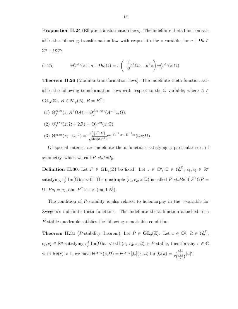
Proposition II.24 (Elliptic transformation laws). The indefinite theta function sat-
isfies the following transformation law with respect to the z variable, for a + Ωb ∈
Zg + ΩZg:
(1.25) Θc1,c2f (z + a+ Ωb; Ω) = e
(−1
2b>Ωb− b>z
)Θc1,c2f (z; Ω).
Theorem II.26 (Modular transformation laws). The indefinite theta function sat-
isfies the following transformation laws with respect to the Ω variable, where A ∈
GLg(Z), B ∈Mg(Z), B = B>:
(1) Θc1,c2f (z;A>ΩA) = ΘAc1,Ac2
f (A−>z; Ω).
(2) Θc1,c2f (z; Ω + 2B) = Θc1,c2
f (z; Ω).
(3) Θc1,c2(z;−Ω−1) =e( 1
2z>Ωz)√
det(iΩ−1)Θ−Ω
−1c1,−Ω
−1c2(Ωz; Ω).
Of special interest are indefinite theta functions satisfying a particular sort of
symmetry, which we call P -stability.
Definition II.30. Let P ∈ GLg(Z) be fixed. Let z ∈ Cg, Ω ∈ H(1)g , c1, c2 ∈ Rg
satisfying c>j Im(Ω)cj < 0. The quadruple (c1, c2, z,Ω) is called P -stable if P>ΩP =
Ω, Pc1 = c2, and P>z ≡ z (mod Z2).
The condition of P -stability is also related to holomorphy in the τ -variable for
Zwegers’s indefinite theta functions. The indefinite theta function attached to a
P -stable quadruple satisfies the following remarkable condition.
Theorem II.31 (P -stability theorem). Let P ∈ GLg(Z). Let z ∈ Cg, Ω ∈ H(1)g ,
c1, c2 ∈ Rg satisfying c>j Im(Ω)cj < 0.If (c1, c2, z,Ω) is P -stable, then for any r ∈ C
with Re(r) > 1, we have Θc1,c2(z,Ω) = Θc1,c2 [fr](z,Ω) for fr(u) = πr+1
2
Γ( r+12 )|u|r.

14
1.3.2 Indefinite zeta functions
Now we state the results on indefinite zeta functions from chapter III. The indef-
inite zeta function has an analytic continuation and functional equation.
Theorem III.3 (Analytic continuation and functional equation). The function ζc1,c2a,b (Ω, s)
may be analytically continued to an entire function on C. It satisfies the functional
equation
(1.26) ζc1,c2a,b
(Ω,g
2− s)
=e(a>b)√det(−iΩ)
ζΩc1,Ωc2−b,a (Ω, s).
The indefinite zeta function may be specialization to differenced zeta functions
attached to ray ideal classes of real quadratic fields.
Theorem III.15 (Specialization of indefinite zeta). For each A ∈ Cc∪∞1,∞2 and
integral ideal b ∈ A−1, there exists a real symmetric matrix M of signature (1, 1),
along with c1, c2, q ∈ C2, such that
(1.27) (2πN(b))−sΓ(s)ZA(s) = ζc1,c20,q (iM, s).
The indefinite zeta function also has a general series expansion—given in Theo-
rem III.11—which involves hypergeometric functions and is not a Dirichlet series.
1.3.3 Kronecker limit formulas
In Chapter IV, we derive a Kronecker limit formula for indefinite zeta functions
in dimension g = 2. The classical “second” Kronecker limit formula for definite zeta
functions, stated in our notation, is as follows.
Proposition IV.3 (Second Kronecker limit formula). Let p =
(p1
p2
)∈ R2 \Z2 and
Ω = iM = iIm(τ)
(1 Re(τ)
Re(τ) ττ
)for τ ∈ H. Then,
ζp,0(Ω, 1) = −2 log
∣∣∣∣∣up21/2+1/12
(v1/2 − v−1/2
) ∞∏d=1
(1− udv
) (1− udv−1
)∣∣∣∣∣(1.28)

15
where u = e(τ) and v = e(p2 − p1τ). This formula may be written more compactly
as
ζp,0(Ω, 1) = −2 log
∣∣∣∣∣ϑ 12
+p2,12−p1
(τ)
η(τ)
∣∣∣∣∣ .(1.29)
This thesis generalizes Proposition IV.3 to arbitrary Ω ∈ H(0)2 .
Theorem IV.1 (Generalized second Kronecker limit formula). Let p =
(p1
p2
)∈ R2
with 0 ≤ p1, p2 < 1, and let Ω = N + iM ∈ H(0)2 . Let z = τ1 and z = τ2 be the
solutions of QΩ
(z
1
)= 0 in the upper and lower half-planes, respectively. Then,
ζp,0(Ω, 1) =−1√
det(−iΩ)((log fp) (τ1) + (log fp) (−τ2)) ,(1.30)
where the function fp : H→ C may be written either of the following ways,
fp(τ) = e(−p2
2
)up
21/2+1/12τ
(v1/2τ − v−1/2
τ
) ∞∏d=1
(1− udτvτ
) (1− udτv−1
τ
)(1.31)
=e((p1 − 1
2
) (p2 + 1
2
))ϑ 1
2+p2,
12−p1
(τ)
η(τ),(1.32)
where uτ = e(τ), vτ = e(p2 − p1τ), ϑ is the Jacobi theta function, and η is the
Dedekind eta function. Here Log fp is the branch satisfying
(1.33) (Log fp)(τ) ∼ πi
(p2
1 − p1 +1
6
)τ as τ → i∞.
Our main result in chapter IV is the following new Kronecker limit formula for
indefinite zeta functions. It involves an integral of a rapidly convergent infinite
product against a function κcΩ
(ξ
1
)built out polynomials and square roots.
Definition IV.5. Suppose Ω = N + iM ∈ H(1)2 , c ∈ C2, and s ∈ C. Let Λc =
Ω− iQM (c)
Mcc>M . Then, we define, for v =
(v1
v2
)∈ C2,
(1.34) κcΩ(v) =c>Mv
4πi√−QM(c)QΩ(v)
√−2iQΛc(v)
.

16
The formula is as follows.
Theorem IV.6 (Indefinite Kronecker limit formula). Let Ω = N + iM ∈ H(1)2 ,
p =
(p1
p2
)∈ R2, and c1, c2 ∈ C2 such that cj
>Mcj < 0. For c = c1, c2, factor the
quadratic form
(1.35) QΛc
(ξ
1
)= α(c)(ξ − τ+(c))(ξ − τ−(c)),
where τ+(c) is in the upper half-plane and τ−(c) is in the lower half-plane. Then,
ζc1,c2p,0 (Ω, 1) = I+(c2)− I−(c2)− I+(c1) + I−(c1),(1.36)
where
I±(c) = −Li2(e(±p1))κcΩ
(1
0
)
+ 2i
∫ ∞0
(Logϕp1,±p2) (±τ±(c) + it)κcΩ
(± (τ±(c) + it)
1
)dt.(1.37)
The function ϕp1,p2 : H→ C is defined by the a product expansion,
(1.38) ϕp1,p2(ξ) := (1− e(p1ξt + p2))∞∏d=1
1− e ((d+ p1)ξ + p2)
1− e ((d− p1)ξ − p2),
and its logarithm (Logϕp1,p2) (ξ) is the unique continuous branch with the property
(1.39) limξ→i∞
(Logϕp1,p2) (ξ) =
log(1− e(p2)) if p1 = 0,
0 if p1 6= 0.
Here log(1− e(p2)) is the standard principal branch.
The following specialization looks somewhat simpler and contains all of the cases
of arithmetic zeta functions ZA(s) associated to real quadratic fields.
Theorem IV.7 (Indefinite Kronecker limit formula, pure imaginary case). Let M
be a 2× 2 real matrix of signature (1, 1), and let Ω = iM . Let p =
(p1
p2
)∈ R2, and
c1, c2 ∈ R2 such that c>j Mcj < 0.
ζc1,c2p,0 (Ω, 1) = 2i Im (I(c2)− I(c1)) ,(1.40)

17
where
I(c) = −Li2(e(p1))κcΩ
(1
0
)(1.41)
+ 2i
∫ ∞0
(Logϕp1,p2) (τ(c) + it)κcΩ
(τ(c) + it
1
)dt.(1.42)
Here, Logϕp1,p2 and κcΩ are defined as in the statement of Theorem IV.6, and ξ = τ(c)
is the unique root of the quadratic polynomial QΛc
(ξ
1
)in the upper half plane.
1.4 Applications to the Stark conjectures
The rank 1 abelian Stark conjecture is known when K = Q or K is an imaginary
quadratic field. It is not known for any other particular base field (e.g., it is open
for K = Q(√
3)). We give a statment of the rank 1 abelian Stark conjecture for
real quadratic fields in terms of the functions ZA(s). Precisely, the following is a
restatement of Conjecture 1 from [44] in the real quadratic case, along with two
addional requirements—Conjecture 2 of [44] and the assumption (included in the
general conjecture in [45]) that the isomorphism between the ray class group and the
Galois group is the Artin map.
Conjecture I.2 (Stark conjecture, rank 1 real quadratic case). Let c be a nonzero
ideal of the ring of integers of a real quadratic number field K with the property that,
if ε ∈ OK such that ε ≡ 1 (mod c), then one of ε or −ε is totally positive. Let A
be a ray ideal class in Clc∪∞2. Let Hj be the ray class field of K modulo c ∪ ∞j,
and let ρj be an embedding of Hj that embeds K using the jth real place, so that
ρ1(H2) = ρ2(H1) is a real field and ρ1(H1) = ρ2(H2) is complex. Then,
(1) Z ′A(0) = log(ρ1(εA)) for a unit εA ∈ H2.
(2) The units εA are compatible with the Artin map Art : Clc∪∞2 → Gal(H/K).
Specifically, εA = εArt(A)I .

18
Our Kronecker limit formula for indefinite zeta functions specializes to an analytic
formula for rank 1 “Stark units” over a real quadratic base field. It deals with the
same cases as Shintani’s Kronecker limit formula [38], although our formula is very
different. It can be used for numerical computation of special values. So far, we have
not been able to obtain any results on algebraicity by these methods.
1.4.1 Stark conjecture example
Now we consider an example. Let K = Q(√
3). The ring of integers is OK =
Z[√
3], and OK has class number 1. A rational prime p 6= 3 splits in K if and only if
p ≡ ±1 (mod 12), by quadratic reciprocity. In particular, (5) is inert, so c = 5OK is
a prime ideal in K. Let ρ1 be the real embedding sending√
3 7→√
3 (determining the
infinite place∞1), and let ρ2 be the real embedding sending√
3 7→ −√
3 (determining
the infinite place ∞2).
The fundamental unit of OK is εK := 2 +√
3. Since OK has class number 1,
Clc∪∞2 may be identified with (OK/c)× × R×/R×+ modulo the action of the unit
group ±(2 +√
3)n : n ∈ Z. We can use −1 to get into R×+, so we’re left with
(OK/c)×/⟨2 +√
3⟩. But (OK/c)× is a cyclic group of order 24, and (2 +
√3)3 =
26 + 15√
3 ≡ 1 (mod 5) so 2 +√
3 has order 3 modulo 5; thus, Clc∪∞2∼= Z/8Z.
Let H2 be the ray class field of OK for Clc∪∞2. The field H2 is unramified at
∞1—that is, a real field with respect to any embedding extending ρ1—but ramified
at ∞2—that is, complex with respect to some (indeed, all) embeddings extending
ρ2. We calculated (with the help of Magma) the intermediate fields between K and
H2, each a quadratic extension of the previous one.
• K = Q(√
3),
• L = K(√
5),

19
• M = L
(√2(5 +√
5))
,
• H2 = M
(√−5 + 10
√3 +√
5 + 2√
15 + (3−√
3 +√
5)√
2(5 +√
5)
).
As expected, that L and M are totally real, whereas H2 is real but not totally real.
In chapter III, we will check the Stark conjecture numerically in this case using a
rapidly convergent formula for the analytic continuation of indefinite zeta functions.
We will see that, if I is the identity element of Clc∪∞2, then
exp (Z ′I(0)) = 3.8908617139430792553376...(1.43)
is equal (to 100 digits) to an algebraic unit, specifically, a root of the polynomial
x8 − (8 + 5√
3)x7 + (53 + 30√
3)x6 − (156 + 90√
3)x5 + (225 + 130√
3)x4
− (156 + 90√
3)x3 + (53 + 30√
3)x2 − (8 + 5√
3)x+ 1.(1.44)
This unit generates the field H2 over K.
In Chapter IV, we will numerically check our Kronecker limit formula in this case
and observe at least 30 decimal places of agreement.
1.5 Applications to SIC-POVMs
The existence of symmetric informationally complete positive operator-valued
measures (SIC-POVMs) in every dimension was conjectured by Zauner in 1999 [53]
and remains open. Much of the progress on this problem has been in the form of
numerical investigations—enumerating all or some of the SIC-POVMs in particular
dimensions. The numerical evidence strongly supports a surprising connection be-
tween SIC-POVMs and Hilbert’s 12th problem for real quadratic fields discovered
numerically by Appleby, Flammia, McConnell and Yard [5, 6].
An SIC-POVM is a set of d2 “equiangular complex lines” in d-dimensional Hilbert
space. In other words, it is a set of one-dimensional subspaces Cv1,Cv2, . . . ,Cvd2 ⊂

20
Cd such that∣∣∣ 〈vi,vj〉2〈vi,vi〉〈vj ,vj〉
∣∣∣ takes the same value for all i 6= j. It is known that
at most d2 complex lines can be equiangular in Cd. Moreover, it is known that∣∣∣ 〈vi,vj〉2〈vi,vi〉〈vj ,vj〉
∣∣∣ = 1d+1
in this case.
It is conjectured that SIC-POVMs exist in every dimension, and that there are
only finitely many in each dimension except for d = 3. Moreover, it is conjectured
that, excluding exceptions in dimensions d = 2, 4, 8, all SIC-POVMs are unitary-
equivalent to Heisenberg SIC-POVMs, which are the orbit of a fiducial vector under
the action of a certain Heisenberg group.
SIC-POVMs were introduced by Zauner in 1999 in his Ph.D. thesis [53] (translated
[54] into English from German in 2011). SIC-POVMs appear in quantum informa-
tion processing (e.g., [46, 11]) and quantum foundations (specifically the theory of
quantum Baysianism [18]), and they have been connected to Lie and Jordan algebras
[3, 4]. Computer calculations by Scott and Grassl have found at least one SIC-POVM
in every dimension up to d = 121 [37, 36]. The case d = 4 is described in detail is
[8]. An overview of the SIC-POVM problem is provided by the preprint [17].
1.5.1 SIC-POVM example
The numerical example for the Stark conjecture discussed in section 1.4.1 corre-
sponds to the ray class field associated to the d = 5 Heisenberg SIC-POVM according
to conjectures of Appleby et. al. [6], which are verified in this case. We found nu-
merically that the derivative differenced zeta values Z ′A(0) for the narrow ray class
group of Z[√
3] modulo (5)∞2 can be related to the phase factors of a fiducial vector
for a d = 5 Heisenberg SIC-POVM. This work will be described in chapter V of this
thesis.

CHAPTER II
Indefinite Theta Functions
In this chapter, we give a theory of indefinite theta functions. For compari-
son, we first provide an overview of the classical theory of Riemann (definite) theta
functions, which are attached to complex symmetric matrices whose imaginary part
defines a quadratic form of signature (g, 0). We then define analogous indefinite
theta functions attached to complex symmetric matrices whose imaginary part de-
fines a quadratic form of signature (g − 1, 1). Our definition is a generalization of
the definition of indefinite theta functions provided in Zwegers’s thesis [56].
This thesis treats theta functions as explicit functions of several complex variables
and doesn’t rely formally on any results from algebraic geometry. However, we will
give an overview of the geometric role of these functions to provide context.
2.1 Riemann theta functions
The definite theta function—or Riemann theta function—of genus g is a function
of an elliptic parameter z and a modular parameter Ω. Riemann’s theory generalizes
the “genus 1” case of Jacobi theta functions. The elliptic parameter z lives in Cg,
but may (almost) be treated as an element of a complex torus Cg/Λ, which happens
to be an abelian variety. The parameter Ω is written as a complex g × g matrix
and lives in the Siegal upper half-space Hg, whose definition imposes a condition on
21

22
M = Im(Ω).
2.1.1 Definitions and geometric context
An abelian variety over a field K is a connected projective algebraic group; it
follows from this definition that the group law of is abelian. (See [31] as a reference
for all results mentioned in this discussion.) A principal polarization on an abelian
variety A is an isomorphism between A and the dual abelian variety A∨. OverK = C,
every principally polarized abelian variety of dimension g is a complex torus of the
form A(C) = Cg/(Zg + ΩZg), where Ω is in the Siegel upper half-space (sometimes
called the Siegel upper half-plane, although it is a complex manifold of dimension
g(g+1)2
).
Definition II.1. The Siegel upper half-space of genus g is defined to be the following
open subset of the space Mg(C) of symmetric g × g complex matrices.
(2.1) H(0)g = Hg = Ω ∈Mg(C) : Ω = Ω> and Im(Ω) is positive-definite.
When g = 1, we recover the usual upper half-plane H1 = H = τ ∈ C : Im(τ) > 0.
Definition II.2. The definite (Riemann) theta function is, for z ∈ Cg and Ω ∈ Hg,
(2.2) Θ(z; Ω) =∑n∈Zg
e
(1
2n>Ωn+ n>z
).
Definition II.3. When g = 1, the definite theta functions is called a Jacobi theta
function and is denoted by ϑ(z, τ) = Θ([z], [τ ]) for z ∈ C and τ ∈ H.
It is a theorem that the complex structure on A(C) determines the algebraic
structure on AC. The functions Θ(z + t; Ω) for representatives t ∈ Cg of 2-torsion
points of A(C) may be used to define an explicit holomorphic embedding of A as an
algebraic locus in complex projective space. These shifts t are called characteristics.
More details may be found in Chapter VI of [28], in particular pages 104–108.

23
The positive integer g is called the “genus” because the Jacobian Jac(C) of an
algebraic curve of genus g is a principally polarized abelian variety of dimension g.
Not all principally polarized abelian varieties are Jacobians of curves; the question
of characterizing the locus of Jacobians of curves inside the moduli space of all
principally polarized abelian varieties is known as the Schottky problem.
2.1.2 A canonical square root
On the Siegel upper half-space Hg, det(−iΩ) has a canonical square root.
Lemma II.4. Let Ω ∈ Hg. Then,
(2.3)
(∫x∈Rg
e
(1
2x>Ωx
)dx
)2
=1
det(−iΩ).
Proof. Equation (2.3) holds for Ω diagonal and purely imaginary by reduction to
the one-dimensional case∫∞−∞ e
−πax2dx = 1√
a. Consequently, eq. (2.3) holds for any
purely imaginary Ω by a change of basis, using spectral decomposition.
Consider the two sides of eq. (2.3) as holomorphic functions in g(g+1)2
complex
variables (the entries of Ω); they agree whenever those g(g+1)2
variables are real.
Because they are holomorphic, it follows by analytic continuation that they agree
everywhere.
Definition II.5. Lemma II.4 provides a canonical square root of det(−iΩ):
√det(−iΩ) :=
(∫x∈Rg
e
(1
2x>Ωx
)dx
)−1
.(2.4)
Whenever we write “√
det(−iΩ)” for Ω ∈ Hg, we will be referring to this square
root.
We will later need to use this square root to evaluate a shifted version of the
integral that defines it.

24
Corollary II.6. Let Ω ∈ Hg and c ∈ Cg. Then,
(2.5)
∫x∈Rg
e
(1
2(x+ c)>Ω(x+ c)
)dx =
1√det(−iΩ)
.
Proof. Fix Ω. The left-hand side of eq. (2.5) is constant for c ∈ Rg, by Lemma II.4.
Because the left-hand side is holomorphic in c, it is in fact constant for all c ∈ Cg.
Note that, if Ω ∈ Hg, then Ω is invertible and −Ω−1 ∈ Hg. This is a special case
of Proposition II.15, which says, in particular, that Hg is closed under the fractional
linear transformation action of the symplectic group,
(2.6)
(A BC D
)· Ω = (AΩ +B)(CΩ +D)−1 for
(A BC D
)∈ Spg(R).
In particular,
(0 −II 0
)· Ω = −Ω−1.
The behavior of our canonical square root under the modular transformation
Ω 7→ −Ω−1 is given by the following proposition.
Proposition II.7. If Ω ∈ Hg, then√
det(−iΩ)√
det(iΩ−1) = 1.
Proof. This follows from Definition II.5 by plugging in Ω = iI, because the expression√det(−iΩ)
√det(iΩ−1) is a continuous function of Ω, and Hg is connected.
2.1.3 Transformation laws of definite theta functions
Proposition II.8. The definite theta function for z ∈ Cg and Ω ∈ Hg satisfies the
following transformation law with respect to the z variable, for a+ Ωb ∈ Zg + ΩZg:
(2.7) Θ(z + a+ Ωb,Ω) = e
(−1
2b>Ωb− b>z
)Θ(z,Ω).
Proof. The proof is a straightforward calculation. It may be found (using slightly
different notation) as Theorem 4 on page 8–9 of [34].

25
Theorem II.9. The definite theta function for z ∈ Cg and Ω ∈ Hg satisfies the
following transformation laws with respect to the Ω variable, where A ∈ GLg(Z),
B ∈Mg(Z), B = B>:
(1) Θ(z;A>ΩA) = Θ(A−>z; Ω).
(2) Θ(z; Ω + 2B) = Θ(z; Ω).
(3) Θ(z;−Ω−1) =e( 1
2z>Ωz)√
det(iΩ−1)Θ(Ωz; Ω).
Proof. The proof of (1) and (2) is a straightforward calculation. A more powerful
version of this theorem, combining (1)–(3) into a single transformation law, appears
as Theorem A on pages 86–87 of [34].
To prove (3), we apply the Poisson summation formula directly to the theta series.
The Fourier transforms of the terms are given as follows.∫Rge(QΩ(n) + n>z
)e(−n>ν
)dn
=
∫Rge(QΩ(n) + n>(z − ν)
)(2.8)
= e (−Q−Ω−1(z − ν))
∫Rge(QΩ
(n+ Ω−1(z − ν)
))(2.9)
=e (−Q−Ω−1(z − ν))√
det(−iΩ).(2.10)
In the last line, we used Lemma II.4 and Definition II.5. Now, by the Poisson
summation formula,
Θ(z,Ω) =∑ν∈Zg
e (−Q−Ω−1(z − ν))√det(−iΩ)
(2.11)
=e (Q−Ω−1(z))√
det(−iΩ)
∑ν∈Zg
e(Q−Ω−1(ν) + ν>Ω−1z
)(2.12)
=e (Q−Ω−1(z))√
det(−iΩ)
∑ν∈Zg
e(Q−Ω−1(ν)− ν>Ω−1z
)(sending ν 7→ −ν)(2.13)
=e(−1
2z>Ω−1z
)√det(−iΩ)
Θ(−Ω−1z,−Ω−1
).(2.14)

26
If Ω is replaced by −Ω−1, we obtain (3).
As was mentioned, it is possible to combine all of the modular transformations
into a single theorem describing the transformation of Ω under the action of Sp2g(Z),
(2.15)
(A BC D
)· Ω = (AΩ +B)(CΩ +D)−1.
This is already complicated in genus g = 1, where the tranformation law involves
Dedekind sums. The general case is done in Chapter III of [34], with the main
theorems stated on pages 86–90.
2.1.4 Definite theta functions with characteristics
There is another notation for theta functions, using “characteristics,” and it will
be necessary to state the transformation laws using this notation as well. We replace
z with z = p + Ωq for real variables p, q ∈ Rg. The reader is cautioned that the
literature on theta functions contains conflicting conventions, and some authors may
use notation identical to this one to mean something slightly different.
Definition II.10. Define the definite theta null with real characteristics p, q ∈ Rg,
for Ω ∈ Hg:
Θp,q(Ω) = e
(1
2q>Ωq + p>q
)Θ (p+ Ωq,Ω) .(2.16)
The transformation laws for Θp,q(Ω) follow from those for Θ(z,Ω).
Proposition II.11. Let Ω ∈ Hg and p, q ∈ Rg. The elliptic transformation law for
the definite theta null with real characteristics is given by
(2.17) Θp+a,q+b(Ω) = e(a>(q + b)
)Θp,q(Ω).
for a, b ∈ Zg.

27
Proposition II.12. Let Ω ∈ Hg and p, q ∈ Rg. The modular transformation laws
for the definite theta null with real characteristics are given as follows, where A ∈
GLg(Z), B ∈Mg(Z), and B = B>.
(1) Θp,q(A>ΩA) = ΘA−>p,Aq(Ω).
(2) Θp,q(Ω + 2B) = e(−q>Bq)Θp+2Bq,q(Ω).
(3) Θp,q (−Ω−1) =e(p>q)√det(iΩ−1)
Θ−q,p(Ω).
2.2 Indefinite theta functions
If we allow Im(Ω) to be indefinite, the series expansion in eq. (2.2) no longer
converges anywhere. We want to remedy this problem by inserting a variable co-
efficient into each term of the sum. In Chapter 2 of his Ph.D. thesis [56], Sander
Zwegers found—in the case when Ω is purely imaginary—a choice of coefficients that
preserves the transformation properties of the theta function.
The results of this section generalize Zwegers’s work by replacing Zwegers’s indef-
inite theta function ϑc1,c2M (z, τ) by the indefinite theta function Θc1,c2Ω [f ](z,Ω). The
function has been generalized in the following ways.
• Replacing τM for τ ∈ H and M ∈Mg(R) real symmetric in of signature (g−1, 1)
by Ω ∈ H(1)g . (Adds g(g+1)
2− 1 real dimensions.)
• Allowing c1, c2 to be complex. (Adds 2g − 2 real dimensions.)
• Allowing a test function f(u), which must be specialized to f(u) = 1 for all the
modular transformation laws to hold.
One motivation for introducing a test function f is to find transformation laws for
a more general class of test functions (e.g., polynomials). We may investigate the
behavior of test functions under modular transformations in future work.

28
2.2.1 The Siegel intermediate half-space
Definition II.13. If M ∈ GLg(R) and M = M>, the signature of M (or of the
quadratic form QM) is a pair (j, k), where j is the number of positive eigenvalues of
M , and k is the number of negative eigenvalues (so j + k = g).
Definition II.14. For 0 ≤ k ≤ g, we define the Siegel intermediate half-space of
genus g and index k to be
(2.18) H(k)g = Ω ∈Mg(C) : Ω = Ω> and Im(Ω) has signature (g − k, k).
We call a complex torus of the form TΩ = Cg/(Zg + ΩZg) for Ω ∈ H(k)g , k 6= 0, g, an
intermediate torus.
Intermediate tori are usually not algebraic varieties. An example of intermediate
tori in the literature are the intermediate Jacobians of Griffiths [19, 20, 21]. Inter-
mediate Jacobians generalize Jacobians of curves, which are abelian varieties, but
those defined by Griffiths are usually not algebraic. (In contrast, the intermediate
Jacobians defined by Weil [48] are algebraic.)
The symplectic group Sp2g(R) acts on the set of g×g complex symmetric matrices
by the fractional linear transformation action,
(2.19)
(A BC D
)· Ω = (AΩ +B)(CΩ +D)−1.
Proposition II.15. If Ω ∈ H(k)g and
(A BC D
)∈ Sp2g(R), then (AΩ + B)(CΩ +
D)−1 ∈ H(k)g . Moreover, the H
(k)g are the open orbits of the Sp2g(R)-action on the set
of g × g complex symmetric matrices.
Proof. Trivial for
(I B0 I
). For
(A> 00 A−1
), this is Sylvester’s Law of Inertia.
For
(0 −II 0
), we have Im(−Ω−1) = 1
2i(−Ω−1 + Ω
−1) = 1
2iΩ−1
(−Ω + Ω)Ω−1 =

29
Ω−1
Im(Ω)Ω−1 =(
Ω−1)>
Im(Ω)Ω−1, so Im(−Ω−1) and Im(Ω) have the same signa-
ture. These three types of matrices generate Sp2g(R).
Now suppose Ω1,Ω2 ∈ H(k)g . There exists a matrix A ∈ GLg(R) such that
A> Im(Ω1)A = Im(Ω2). For an appropriate choice of real symmetric B ∈Mg(R), we
thus have A>Ω1A+B = Ω2. That is,
(2.20)
(I B0 I
)·(A> 00 A−1
)· Ω1 = Ω2,
so Ω1 and Ω2 are in the same Sp2g(R)-orbit.
Thus, the H(k)g are the open orbits of the Sp2g(R)-action on the set of g × g
symmetric complex matrices.
2.2.2 More canonical square roots
From now on, we will focus on the case of index k = 1, which is signature (g −
1, 1). The construction of modular theta series for k ≥ 2 utilizes higher-order error
functions arising from physics [1]. More research is needed to develop the higher
index theory.
Lemma II.16. Let M be a real symmetric matrix of signature (g − 1, 1). On the
region RM = z ∈ Cg : z>Mz < 0, there is a canonical choice of holomorphic
function g(z) such that g(z)2 = −z>Mz.
Proof. By Sylvester’s law of inertia, there is some P ∈ GL+g (R) (i.e., with det(P ) >
0) such that M = P>JP , where
(2.21) J =
−1 0 0 . . . 0
0 1 0 . . . 0
0 0 1 . . . 0
......
.... . .
...
0 0 0 . . . 1
.

30
The region S = (z2, . . . , zg) ∈ Cg−1 : |z2|2+· · · |zg|2 < 1 is simply connected (as it is
a solid ball) and does not intersect (z2, . . . , zg) ∈ Cg−1 : z22 + · · ·+ z2
g = 1 (because,
if it did, we’d have 1 =∣∣z2
2 + · · ·+ z2g
∣∣ ≤ |z2|2 + · · · |zg|2 < 1, a contradiction).
Thus, there exists a unique continuous function√
1− z22 − · · · − z2
g on S sending
(0, . . . , 0) 7→ 1; this function is also holomorphic. For z ∈ RJ , define
(2.22) gJ(z) := z1
√1−
(z2
z1
)2
− · · · −(zgz1
)2
.
This gJ is holomorphic and satisfies gJ(z)2 = −z>Jz, gJ(αz) = αgJ(z), and gJ(e1) =
1 where
(2.23) e1 =
1
0
...
0
.
Conversely, if we have a continuous function g(z) satisfying g(z)2 = −z>Jz and
g(e1) = 1, it follows that g(αz) = αg(z), and thus g(z) = gJ(z).
Now, we’d like to define gM(z) := gJ(Pz), so that we have gM(z)2 = −z>Mz.
We need to check that this definition does not depend on the choice of P . Suppose
M = P>1 JP1 = P>2 JP2 for P1, P2 ∈ GL+g (R). So J =
(P2P
−11
)>J(P2P
−11
), that
is, P2P−11 ∈ O(g − 1, 1). But det(P2P
−11 ) = det(P2) det(P1)−1 > 0, so, in fact,
P2P−11 ∈ SO(g − 1, 1).
For any Q ∈ SO(g−1, 1), we have gJ(Qe1)2 = 1. The function Q 7→ gJ(Qe1) must
be either the constant 1 or the constant −1, because SO(g−1, 1) is connected. Since
gJ(e1) = 1 (Q = I), we have gJ(Qe1) = 1 for all Q ∈ SO(1, g − 1). The function
z 7→ gJ(Qz) is a continuous square root of −z>Jz sending e1 to 1, so gJ(Qz) =
gJ(z). Taking Q = P2P−11 and replacing z with P1z, we have gJ(P2z) = gJ(P1z), as
desired.

31
Definition II.17. If M is a real symmetric matrix of signature (g − 1, 1), we will
write√−z>Mz for the function gM(z) in Lemma II.16. We may also use similar
notation, such as√−1
2z>Mz := 1√
2
√−z>Mz.
Lemma II.18. Suppose M is a real symmetric matrix of signature (g − 1, 1), and
c ∈ Cg such that c>Mc < 0. Then, M +M Re((−1
2c>Mc
)−1cc>)M is well-defined
(that is, c>Mc 6= 0) and positive definite.
Proof. Because M has signature (g − 1, 1) and c>Mc < 0,
(c>Mc
)2 −∣∣c>Mc
∣∣2 = det
(c>Mc c>Mcc>Mc c>Mc
)< 0.(2.24)
Thus,∣∣c>Mc
∣∣ > (c>Mc)2> 0, so c>Mc 6= 0 and M + M Re
((−1
2c>Mc
)−1cc>)M
is well defined. Let
A = M +M Re
((−1
2c>Mc
)−1
cc>
)M(2.25)
= M −M(c>Mc
)−1cc>M −M
(c>Mc
)−1cc>M.(2.26)
On the (g − 1)-dimensional subspace W = w ∈ Cg : c>Mw = 0, the sesquilinear
form w 7→ w>Mw is positive definite; this follows from the fact that c>Mc < 0,
because M has signature (g − 1, 1). For nonzero w ∈ W ,
w>Aw = w>Mw − (c>Mc)−1(w>Mc)(c>Mw)− (c>Mc)−1(w>Mc)(c>Mw)(2.27)
= w>Mw − (c>Mc)−1(0)(c>Mw)− (c>Mc)−1(w>Mc)(0)(2.28)
= w>Mw > 0.(2.29)
Moreover,
c>Aw = c>Mw − (c>Mc)−1(c>Mc)(c>Mw)− (c>Mc)−1(c>Mc)(c>Mw)(2.30)
= c>Mw − c>Mw − (c>Mc)−1(c>Mc)(0)(2.31)
= 0,(2.32)

32
and
c>Ac = c>Mc− (c>Mc)−1(c>Mc)(c>Mc)− (c>Mc)−1(c>Mc)(c>Mc)(2.33)
= c>Mc− c>Mc− c>Mc(2.34)
= −c>Mc(2.35)
= −c>Mc > 0.(2.36)
We have now shown that A is positive definite, as it is positive definite on subspaces
W and Cc, and these subspaces span Cg and are perpendicular with respect to A.
Lemma II.19. Let Ω = N + iM be an invertible complex symmetric g × g matrix.
Consider c ∈ Cg such that c>Mc < 0. The following identities hold:
(1) MΩ−1 = Ω Im (−Ω−1).
(2) M − 2iMΩ−1M = Ω Im (−Ω−1) Ω.
(3) det(−i(Ω− 2i
c>McMcc>M
))= det(−iΩ)
c>Ω Im(−Ω−1)Ωc
c>Mc.
Proof. Proof of (1):
MΩ−1 =1
2i(Ω− Ω)Ω−1(2.37)
=1
2i(I − ΩΩ−1)(2.38)
= Ω1
2i(Ω−1 − Ω−1)(2.39)
= Ω Im(−Ω−1
).(2.40)
Proof of (2):
M − 2iMΩ−1M = MΩ−1 (Ω− 2iM)(2.41)
= Ω Im(−Ω−1
) (Ω− (Ω− Ω)
)using (1)(2.42)
= Ω Im(−Ω−1
)Ω.(2.43)

33
Proof of (3): Note that det(I + A) = 1 + Tr(A) for any rank 1 matrix A. Thus,
det
(−i(
Ω− 2i
c>McMcc>M
))(2.44)
= det(−iΩ) det
(I +
2i
c>Mc(ΩMc)(Mc)>
)(2.45)
= det(−iΩ)
(1 + Tr
(2i
c>Mc(ΩMc)(Mc)>
))(2.46)
= det(−iΩ)
(1 +
(2i
c>Mcc>MΩ−1Mc
))(2.47)
= det(−iΩ)−c> (M − 2iMΩ−1M) c
−c>Mc(2.48)
= det(−iΩ)−(Ωc)> Im (−Ω−1) (Ωc)
−c>Mc,(2.49)
using (2) in the last step.
Definition II.20 (Canonical square root). If Ω ∈ H(1)g , then we define
√det(−iΩ)
as follows. Write Ω = N + iM for N,M ∈ Mg(R), and choose any c such that
c>Mc < 0. By Lemma II.18, M + M Re((−1
2c>Mc
)−1cc>)M is positive definite.
Write M + M Re((−1
2c>Mc
)−1cc>)M = Im
(Ω− 2i
c>McMcc>M
). By part (3) of
Lemma II.19,
(2.50) det
(−i(
Ω− 2i
c>McMcc>M
))= det(−iΩ)
−(Ωc)> Im (−Ω−1) (Ωc)
−c>Mc.
We can thus define√
det(−iΩ) as follows:
(2.51)√
det(−iΩ) :=
√−c>Mc
√det(−i(Ω− 2i
c>McMcc>M
))√−(Ωc)> Im (−Ω−1) (Ωc)
,
where the square roots on the RHS are as defined in Definition II.5 and Defini-
tion II.17. This definition does not depend on the choice of c because the set
c ∈ Cg : c>Mc < 0 is connected.

34
2.2.3 Definition of indefinite theta functions
Definition II.21. For any complex number α and any entire test function f , define
the incomplete Gaussian transform
Ef (α) =
∫ α
0
f(u)e−πu2
du,(2.52)
where the integral may be taken along any contour from 0 to α. In particular, for
the constant functions 1(u) = 1, set
E(α) := E1(α) =
∫ α
0
e−πu2
du =α
2|α|
∫ |α|20
t−1/2e−π(α/|α|)2t dt.(2.53)
When α is real, define Eg(α) for an arbitrary continuous test function f :
Ef (α) =
∫ α
0
f(u)e−πu2
du.(2.54)
Definition II.22. Define the indefinite theta function attached to the test function
f to be
(2.55) Θc1,c2 [f ](z; Ω) =∑n∈ZgEf
c> Im(Ωn+ z)√−1
2c> Im(Ω)c
∣∣∣∣∣∣c2
c=c1
e
(1
2n>Ωn+ n>z
),
where Ω ∈ H(1)g , z ∈ Cg, c1, c2 ∈ Cg, c1
>Mc1 < 0, c2>Mc2 < 0, and f(ξ) is
a continuous function of one variable satisfying the growth condition log |f(ξ)| =
o(|ξ|2). If the cj are not both real, also assume that f is entire.
Also define the indefinite theta function Θc1,c2(z; Ω) := Θc1,c2 [1](z; Ω).
The function Θc1,c2(z; Ω) = Θc1,c2 [1](z; Ω) is the function we are most interested
in, because it will turn out to satisfy a symmetry in Ω 7→ −Ω−1. We will also show
that the functions Θc1,c2 [u 7→ |u|r](z; Ω) are equal (up to a constant) for certain
special values of the parameters.
Before we can prove the transformation laws of our theta functions, we must show
that the series defining them converges.

35
Proposition II.23. The indefinite theta series attached to f (eq. (2.55)) converges
absolutely and uniformly for z ∈ Rg + iK, where K is a compact subset of Rg (and
for fixed Ω, c1, c2, and f).
Proof. Let M = Im Ω. We may multiply c1 and c2 by any complex scalar with-
out changing the terms of the series eq. (2.55), so we may assume without loss of
generality that Re(c1>Mc2) < 0.
For λ ∈ [0, 1], define the vector c(λ) = (1−λ)c1+λc2 and the real symmetric matrix
A(λ) := M + M Re((−1
2c(λ)>Mc(λ)
)−1c(λ)c(λ)>
)M . Note that c(λ)
>Mc(λ) =
(1−λ)2c1>Mc1+2λ(1−λ) Re(c1
>Mc2)+λ2c2>Mc2 < 0 because each term is negative
(except when λ = 0 or 1, in which case one term is negative and the others are zero).
By Lemma II.18, A(λ) is well-defined and positive definite for each λ ∈ [0, 1].
Consider (x, λ) 7→ x>A(λ)x as a positive real-valued continuous function on the
compact set that is the product of the unit ball x>x = 1 and the interval [0, 1]. It
has a global minimum ε > 0.
The parametrization γ : [0, 1] → C, γ(λ) := c(λ)>(Mn+y)√− 1
2c(λ)>Mc(λ)
, defines a countour
fromc>1 (Mn+y)√− 1
2c>1 Mc1
toc>2 (Mn+y)√− 1
2c>2 Mc2
, so that
(2.56) Ef(c>(Mn+ y)
−12c>Mc
)∣∣∣∣c2c=c1
=
∫γ
f(u)e−πu2
du.
We give an upper bound for
maxλ∈[0,1]
∣∣∣∣e−πγ(λ)2
e
(1
2n>Ωn+ n>z
)∣∣∣∣(2.57)
= eπy>M−1y max
λ∈[0,1]e
−π− 1
2 c(λ)>Mc(λ)(c(λ)>M(n+M−1y))
2
e−π(n+M−1y)>M(n+M−1y)(2.58)
= eπy>M−1y max
λ∈[0,1]e−π(n+M−1y)
>A(λ)(n+M−1y)(2.59)
≤ eπy>M−1ye−πε‖n+M−1y‖2
.(2.60)

36
Thus, ∣∣∣∣∣Ef(c>(Mn+ y)
−12c>Mc
)∣∣∣∣c2c=c1
e
(1
2n>Ωn+ n>z
)∣∣∣∣∣≤∫γn
|f(u)| eπy>M−1ye−πε‖n+M−1y‖2
du(2.61)
≤ p(n)e−πε‖n+M−1y‖2
,(2.62)
where log p(n) = o (‖n‖2). Thus, the terms of the series are o(e−
πε2 (‖n‖2+‖M−1y‖)
),
and so the series converges absolutely and uniformly for x ∈ Rg and y ∈ K.
2.2.4 Transformation laws of indefinite theta functions
We will now prove the elliptic and modular transformation laws for indefinite
theta functions. In all of these results, we assume that z ∈ Cg, Ω ∈ H(1)g , cj ∈ Cg
satisfying cj> Im(Ω)cj, and f is a function of one variable satisfying the conditions
specified in Definition II.22.
Proposition II.24. The indefinite theta function attached to f satisfies the following
transformation law with respect to the z variable, for a+ Ωb ∈ Zg + ΩZg:
(2.63) Θc1,c2 [f ](z + a+ Ωb; Ω) = e
(−1
2b>Ωb− b>z
)Θc1,c2 [f ](z; Ω).
Proof. By definition,
Θc1,c2 [f ](z + a+ Ωb; Ω)
=∑n∈ZgEf(c> Im(Ωn+ (z + a+ Ωb))
−12c> Im(Ω)c
)∣∣∣∣c2c=c1
e(QΩ(n) + n>(z + a+ Ωb)
).(2.64)

37
Because a ∈ Zg, Im(a) is zero and e(n>a) = 1, so
Θc1,c2 [f ](z + a+ Ωb; Ω)
=∑n∈ZgEf(c> Im(Ω(n+ b) + z)
−12c> Im(Ω)c
)∣∣∣∣c2c=c1
e(QΩ(n) + n>(z + Ωb)
)(2.65)
= e
(−1
2b>Ωb
)∑n∈ZgEf(c> Im(Ω(n+ b) + z)
−12c> Im(Ω)c
)∣∣∣∣c2c=c1
e(QΩ(n+ b) + n>z
)(2.66)
= e
(−1
2b>Ωb
)∑n∈ZgEf(c> Im(Ωn+ z)
−12c> Im(Ω)c
)∣∣∣∣c2c=c1
e(QΩ(n) + (n− b)>z
)(2.67)
= e
(−1
2b>Ωb− b>z
)Θ[f ]c1,c2(z; Ω).(2.68)
The identity is proved.
Proposition II.25. The indefinite theta function satisfies the following condition
with respect to the c variable:
(2.69) Θc1,c3 [f ](z; Ω) = Θc1,c2 [f ](z; Ω) + Θc2,c3 [f ](z; Ω)
Proof. Add the series termwise.
Theorem II.26. The indefinite theta function satisfies the following transformation
laws with respect to the Ω variable, where A ∈ GLg(Z), B ∈Mg(Z), B = B>:
(1) Θc1,c2 [f ](z;A>ΩA) = ΘAc1,Ac2 [f ](A−>z; Ω).
(2) Θc1,c2 [f ](z; Ω + 2B) = Θc1,c2 [f ](z; Ω).
(3) In the case where f(u) = 1(u) = 1, we have
(2.70) Θc1,c2(z;−Ω−1) =eπiz
>Ωz√det(iΩ−1)
Θ−Ω−1c1,−Ω
−1c2(Ωz; Ω).

38
Proof. The proof of (1) is a direct calculation.
Θc1,c2 [f ](z;A>ΩA)
=∑n∈ZgEf
c> Im(A>ΩAn+ z)√−1
2c> Im(Ω)c
∣∣∣∣∣∣c2
c=c1
e
(1
2n>A>ΩAn+ n>z
)(2.71)
=∑m∈Zg
Ef
c> Im(A>Ωm+ z)√−1
2c> Im(Ω)c
∣∣∣∣∣∣c2
c=c1
e
(1
2m>Ωm+
(A−1m
)>z
)(2.72)
by the change of basis m = An, so
Θc1,c2 [f ](z;A>ΩA)
=∑m∈Zg
Ef
(Ac)> Im(Ωm+ A−>z)√−1
2c> Im(Ω)c
∣∣∣∣∣∣c2
c=c1
e
(1
2m>Ωm+m>A−>z
)(2.73)
= ΘAc1,Ac2 [f ](A−>z; Ω).(2.74)
The proof of (2) is also a direct calculation.
Θc1,c2 [f ](z; Ω + 2B)
=∑n∈ZgEf
c> Im((Ω + 2B)n+ z)√−1
2c> Im(Ω)c
∣∣∣∣∣∣c2
c=c1
e
(1
2n>(Ω + 2B)n+ n>z
)(2.75)
=∑n∈ZgEf
c>(Im((Ω)n+ z)) + 2 Im(B)n√−1
2c> Im(Ω)c
∣∣∣∣∣∣c2
c=c1
e(QΩ(n) + n>Bn+ n>z
)(2.76)
=∑n∈ZgEf
c> Im((Ω)n+ z)√−1
2c> Im(Ω)c
∣∣∣∣∣∣c2
c=c1
e(QΩ(n) + n>z
)(2.77)
= Θc1,c2 [f ](z; Ω);(2.78)
where e(n>Bn
)= 1 because the n>Bn are integers, and Im(B) = 0 because B is a
real matrix.
The proof of (3) is more complicated, and, like the proof of the analogous property
for definite (Jacobi and Riemann) theta functions, uses Poisson summation. The

39
argument that follows is a modification of the argument that appears in the proof of
Lemma 2.8 of Zwegers’s thesis [56].
We will find a formula for the Fourier transform of the terms of our theta series.
Most of the work is done in the calculation of the integral that follows. In this
calculation, M = Im Ω, and z = x+ iy for x, y ∈ Cg. The differential operator Ox is
a row vector with entries ∂∂xj
, and similarly for On.
Ox
∫n∈Rg
E
c>Mn+ c>y√−1
2c>Mc
∣∣∣∣∣∣c2
c=c1
e(QΩ
(n+ Ω−1z
))dn
=
∫n∈Rg
E
c>Mn+ c>y√−1
2c>Mc
∣∣∣∣∣∣c2
c=c1
Ox
(e(QΩ
(n+ Ω−1z
)))dn(2.79)
=
∫n∈Rg
E
c>Mn+ c>y√−1
2c>Mc
∣∣∣∣∣∣c2
c=c1
On
(e(QΩ
(n+ Ω−1z
)))dn
Ω−1(2.80)
=
−∫n∈Rg
On
Ec>Mn+ c>y√
−12c>Mc
∣∣∣∣∣∣c2
c=c1
e(QΩ
(n+ Ω−1z
))dn
Ω−1(2.81)
=
(k
∫n∈Rg
e
(i
−c>Mc
(c> Im(Ω)n
)2)e (QΩ(n+ az)) dn
)c>MΩ−1
∣∣∣∣c2c=c1
,(2.82)
where k = −2√− 1
2c>Mc
∈ C, az = Ω−1z −M−1y ∈ Cg, and integration by parts was
used in eq. (2.81). Continuing the calculation,
Ox
∫n∈Rg
E
c>Mn+ c>y√−1
2c>Mc
∣∣∣∣∣∣c2
c=c1
e(QΩ
(n+ Ω−1z
))dn
= k
(∫n∈Rg
e
(QΩ− 2i
c>McMcc>M(n) + a>Ωn+
1
2a>Ωa
)dn
)c>MΩ−1
∣∣∣∣c2c=c1
(2.83)
= ke
(−1
2a>Ω
(Ω− 2i
c>McMcc>M
)−1
Ωa+1
2a>Ωa
)I(c)c>MΩ−1
∣∣∣∣∣c2
c=c1
,(2.84)

40
where
I(c) =
∫n∈Rg
e
(QΩ− 2i
c>McMcc>M
(n+
(Ω− 2i
c>McMcc>M
)−1
Ωa
))dn(2.85)
=1
det√−i(Ω− 2i
c>McMcc>M
)(2.86)
by Lemma II.4.
We can check (by multiplication) that
(2.87)
(Ω− 2i
c>McMcc>M
)−1
= Ω−1 − 2i
c>Mc− 2ic>MΩ−1McΩ−1Mcc>MΩ−1.
Thus,
(2.88) Ω− Ω
(Ω− 2i
c>McMcc>M
)−1
Ω =2i
c>Mc− 2ic>MΩ−1McMcc>M.
Now compute, using Lemma II.19, Ma = MΩ−1z − y = Ω Im (−Ω−1) z − y =
Ω(
Im (−Ω−1) z − Ω−1y)
= 12i
Ω((−Ω−1 + Ω
−1)z − Ω
−1(z − z)
)= 1
2iΩ(−Ω−1z + Ω
−1z)
=
Ω Im (−Ω−1z) . Also by Lemma II.19, M − 2iMΩ−1M = Ω Im (−Ω−1) Ω, and√det
(−i(
Ω− 2i
c>McMcc>M
))=√
det(−iΩ)
√−c>Ω Im (−Ω−1) Ωc√−c>Mc
.(2.89)
We have now shown that
Ox
∫n∈Rg
E
c> Im (Ωn+ z)√−1
2c>Mc
∣∣∣∣∣∣c2
c=c1
e(QΩ
(n+ Ω−1z
))dn
]nn(2.90)
=−2e
(i
(Ωc) Im(−Ω−1)(Ωc)(c>Ma)2
)√
det(−iΩ)√−1
2(Ωc) Im(−Ω−1)(Ωc)
c>MΩ−1
∣∣∣∣∣∣c2
c=c1
(2.91)
=−2e
(i
(Ωc) Im(−Ω−1)(Ωc)(c>Ma)2
)√
det(−iΩ)√−1
2(Ωc) Im(−Ω−1)(Ωc)
(Ωc)> Im(Ω−1)
∣∣∣∣∣∣c2
c=c1
(2.92)
=1√
det(−iΩ)OxE
(Ωc)> (Im(−Ω−1)n+ Im(−Ω−1z))√−1
2(Ωc) Im(−Ω−1)(Ωc)
∣∣∣∣∣∣c2
c=c1
.(2.93)

41
Define the following function on Cg,
C(z) = C(c)Ω (z) :=
∫n∈RgE
c> Im (Ωn+ z)√−1
2c>Ωc
e(QΩ
(n+ Ω−1z
))dn(2.94)
− 1√det(iΩ)
E
(Ωc)> Im(−Ω−1z)√−1
2(Ωc) Im(−Ω−1)(Ωc)
,(2.95)
suppressing the dependence of C(z) on Ω and c. We have just showed that ∆xC(z) =
0, so C(z + a) = C(z) for any a ∈ Rg. By inspection, C(z + Ω−1b) = C(z) for any
b ∈ Rg. It follow from both of these properties that C(z) is constant. Moreover, by
inspection, C(−z) = −C(z); therefore, C(z) = 0. In other words,∫n∈Rg
E
c> Im (Ωn+ z)√−1
2c>Ωc
∣∣∣∣∣∣c2
c=c1
e(QΩ
(n+ Ω−1z
))dn
=1√
det(−iΩ)E
(Ωc)> Im(−Ω−1z)√−1
2(Ωc) Im(−Ω−1)(Ωc)
∣∣∣∣∣∣c2
c=c1
.(2.96)
Now set g(z) := Θc1,c2(z; Ω), which has Fourier coefficients
(2.97) cn(g)(z) = E
c> Im (Ωn+ z)√−1
2c>Ωc
∣∣∣∣∣∣c2
c=c1
e
(1
2n>Ωn+ n>z
).
By plugging in z−ν for z in eq. (2.96) and multiplying both sides by e(−1
2(z − ν)>Ω−1(z − ν)
),
we obtain the following expression for the Fourier coefficients of g:
cν (g) (z) =
∫n∈Rg
E
c> Im (Ωn+ z)√−1
2c>Ωc
∣∣∣∣∣∣c2
c=c1
e
(1
2n>Ωn+ n>z
)e(−n>ν) dn(2.98)
=e(−1
2(z − ν)>Ω−1(z − ν)
)√det(−iΩ)
E
(Ωc)> Im(−Ω−1ν − Ω−1z)√−1
2(Ωc) Im(−Ω−1)(Ωc)
∣∣∣∣∣∣c2
c=c1
(2.99)
=e(−1
2z>Ω−1z
)√det(−iΩ)
E
(Ωc)> Im(−Ω−1(−ν)− Ω−1z)√−1
2(Ωc) Im(−Ω−1)(Ωc)
∣∣∣∣∣∣c2
c=c1
(2.100)
· e(
1
2ν>(−Ω−1)ν + (−ν)>(−Ω−1z)
).(2.101)

42
It follows by Poisson summation that
Θc1,c2(z; Ω) =∑ν∈Zg
cν (g) (z)(2.102)
=e(−1
2z>Ω−1z
)√det(−iΩ)
ΘΩc1,Ωc2(−Ω−1z;−Ω−1
).(2.103)
We obtain (3) by replacing Ω with −Ω−1.
2.2.5 Indefinite theta functions with characteristics
Now we restate the transformation laws using “characteristics” notation, which
will be used when we define indefinite zeta functions in chapter III.
Definition II.27. Define the indefinite theta null with characteristics p, q ∈ Rg:
Θc1,c2p,q [f ](Ω) = e2πi( 1
2q>Ωq+p>q)Θc1,c2 [f ] (p+ Ωq; Ω) ;(2.104)
Θc1,c2p,q (Ω) = e2πi( 1
2q>Ωq+p>q)Θc1,c2 (p+ Ωq; Ω) .(2.105)
The transformation laws for Θc1,c2p,q [f ](Ω) follow from the transformation laws for
Θc1,c2 [f ](z; Ω).
Proposition II.28. The elliptic transformation law for the indefinite theta null with
characteristics is:
(2.106) Θc1,c2p+a,q+b[f ](Ω) = e(a>(q + b))Θc1,c2
p,q [f ](Ω).
Proposition II.29. The modular transformation laws for the indefinite theta null
with characteristics are as follows.
(1) Θc1,c2p,q [f ](A>ΩA) = ΘAc1,Ac2
A−>p,Aq[f ](Ω).
(2) Θc1,c2p,q [f ](Ω + 2B) = e(−q>Bq)Θc1,c2
p+2Bq,q[f ](Ω).
(3) Θc1,c2p,q (−Ω−1) = e(p>q)√
det(iΩ−1)Θ−Ω
−1c1,−Ω
−1c2
−q,p (Ω).
43
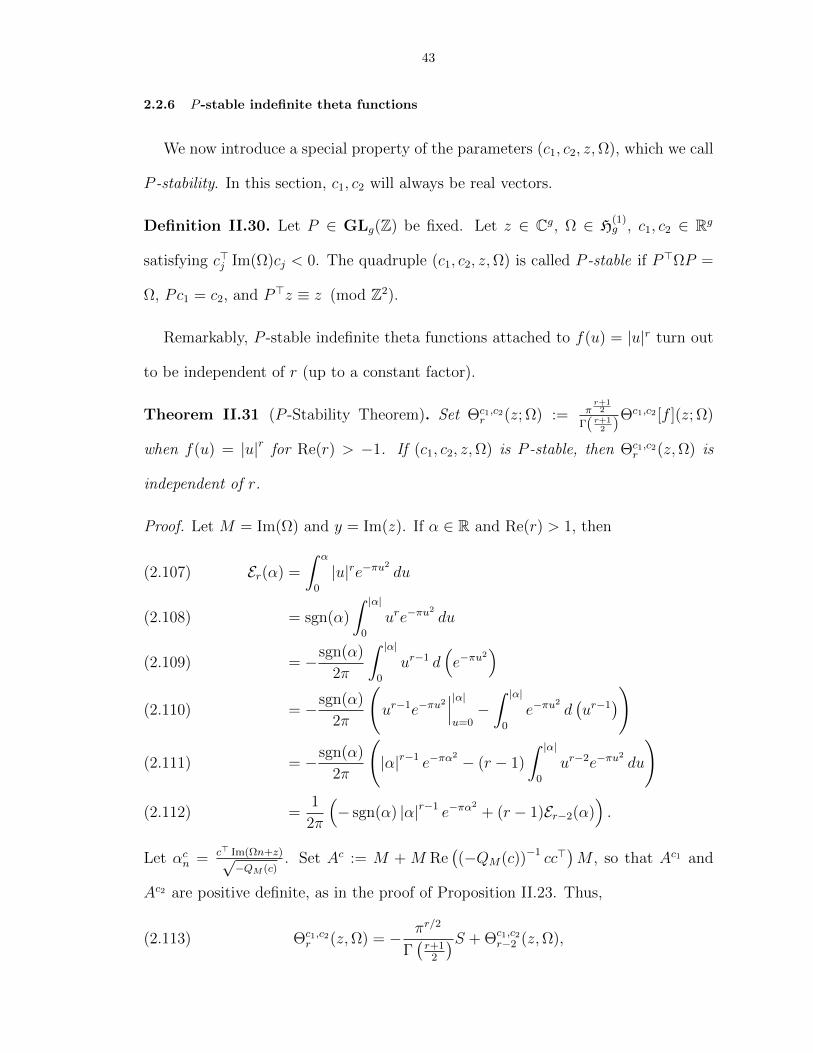
2.2.6 P -stable indefinite theta functions
We now introduce a special property of the parameters (c1, c2, z,Ω), which we call
P -stability. In this section, c1, c2 will always be real vectors.
Definition II.30. Let P ∈ GLg(Z) be fixed. Let z ∈ Cg, Ω ∈ H(1)g , c1, c2 ∈ Rg
satisfying c>j Im(Ω)cj < 0. The quadruple (c1, c2, z,Ω) is called P -stable if P>ΩP =
Ω, Pc1 = c2, and P>z ≡ z (mod Z2).
Remarkably, P -stable indefinite theta functions attached to f(u) = |u|r turn out
to be independent of r (up to a constant factor).
Theorem II.31 (P -Stability Theorem). Set Θc1,c2r (z; Ω) := π
r+12
Γ( r+12 )
Θc1,c2 [f ](z; Ω)
when f(u) = |u|r for Re(r) > −1. If (c1, c2, z,Ω) is P -stable, then Θc1,c2r (z,Ω) is
independent of r.
Proof. Let M = Im(Ω) and y = Im(z). If α ∈ R and Re(r) > 1, then
Er(α) =
∫ α
0
|u|re−πu2
du(2.107)
= sgn(α)
∫ |α|0
ure−πu2
du(2.108)
= −sgn(α)
2π
∫ |α|0
ur−1 d(e−πu
2)
(2.109)
= −sgn(α)
2π
(ur−1e−πu
2∣∣∣|α|u=0−∫ |α|
0
e−πu2
d(ur−1
))(2.110)
= −sgn(α)
2π
(|α|r−1 e−πα
2 − (r − 1)
∫ |α|0
ur−2e−πu2
du
)(2.111)
=1
2π
(− sgn(α) |α|r−1 e−πα
2
+ (r − 1)Er−2(α)).(2.112)
Let αcn = c> Im(Ωn+z)√−QM (c)
. Set Ac := M + M Re((−QM(c))−1 cc>
)M , so that Ac1 and
Ac2 are positive definite, as in the proof of Proposition II.23. Thus,
(2.113) Θc1,c2r (z,Ω) = − πr/2
Γ(r+1
2
)S + Θc1,c2r−2 (z,Ω),

44
where
S =∑n∈Zg
sgn (αcn) |αcn|r−1 exp
(−π (αcn)2)∣∣c2
c=c1e
(1
2n>Ωn+ n>z
).(2.114)
The c1 and c2 terms in this sum decay exponentially, because
(2.115)
∣∣∣∣exp(−π (αcn)2) e(1
2n>Ωn+ n>z
)∣∣∣∣ = exp(−2πQAc
(n+M−1y)
)).
Thus, the series may be split as a sum of two series:
S =∑n∈Zg
sgn (αc2n ) |αc2n |r−1 exp
(−π (αc2n )2) e(1
2n>Ωn+ n>z
)(2.116)
−∑n∈Zg
sgn (αc1n ) |αc1n |r−1 exp
(−π (αc1n )2) e(1
2n>Ωn+ n>z
).(2.117)
Now we use the P -symmetry to show that these two series are, in fact, equal. Note
that Im(P>z) = Im(z) because P>z ≡ z (mod Z2), so
αPn(c2) =(Pc1)> Im(ΩPn+ z)√
−QM(Pc1)(2.118)
=c>1 Im(P>ΩPn+ P>z)√
−QP>MP (c1)(2.119)
=c>1 Im(Ωn+ z)√−QM(c1)
(2.120)
= αn(c1).(2.121)
Moreover,
1
2(Pn)>Ω(Pn) + (Pn)>z =
1
2n>(P>ΩP )n+ n>(P>z)(2.122)
≡ 1
2n>Ωn+ n>z
(mod Z2
).(2.123)
Thus, we may substitute Pn for n in the first series (involving c2) to obtain the
second (involving c1).
We’ve now shown the periodicity relation
(2.124) Θc1,c2r (z,Ω) = Θc1,c2
r−2 (z,Ω).

45
Note that this identity provides an analytic continuation of Θc1,c2r (z,Ω) to the entire
r-plane. To show that it is constant in r, we will show that it is bounded on vertical
strips in the r-plane. As in the proof of Proposition II.23, bound (x, λ) 7→ x>A(λ)x,
considered as a positive real-valued continuous function on the product of the unit
ball x>x = 1 and the interval [0, 1], from below by its global minimum ε > 0.
Thus, ∣∣∣∣∣∣∣Erc>(Mn+ y)√
−12c>Mc
∣∣∣∣∣∣c2
c=c1
e
(1
2n>Ωn+ n>z
)∣∣∣∣∣∣∣≤
∣∣∣∣∣∣∫ c>2 Im(Ωn+z)√
− 12 c>2 Im(Ω)c2
c>1 Im(Ωn+z)√− 1
2 c>1 Im(Ω)c1
|u|Re(r) du
∣∣∣∣∣∣ eπy>M−1ye−πε‖n+M−1y‖2
(2.125)
≤ pRe(r)(n)e−πε‖n+M−1y‖2
,(2.126)
where pRe(r)(n) is a polynomial independent of Im(r). Hence, Θc1,c2r (z,Ω) is bounded
on the line Re(r) = σ by∑
n∈Zg pσ(n)e−πε‖n+M−1y‖2
. It follows that it is bounded on
any vertical strip. Along with periodicity, this implies that Θc1,c2r (z,Ω) as a function
of r is bounded and entire, thus constant.
CHAPTER III
Indefinite Zeta Functions and Real Quadratic Fields
In this chapter, we consider the Mellin transforms of definite and indefinite theta
functions. In the definite case in dimension 2, they are generalize analytic Eisenstein
series, and they specialize to zeta functions of imaginary quadratic ideal classes. In
the indefinite case in dimension 2, we recover certain L-series attached to (ideals
of orders of) real quadratic fields. The class of L-series we recover spans the same
vector space as those Hecke L-functions attached to Hecke characters of finite order
ramified at exactly one infinite place.
3.1 Definite zeta functions and real analytic Eisenstein series
We define the definite zeta function as a Mellin transform of the indefinite theta
null with real characteristics.
Definition III.1. Let Ω ∈ H(0)g and p, q ∈ Rg. The definite zeta function is
(3.1) ζp,q(Ω, s) =
∫∞
0Θp,q(tΩ)ts dt
tif q /∈ Zg,∫∞
0(Θp,q(tΩ)− 1) ts dt
tif q ∈ Zg.
By direct calculation, ζp,q(Ω, s) has a Dirichlet series expansion.
ζp,q(Ω, s) = (2π)−sΓ(s)∑n∈Zgn6=−q
e(p>(n+ q))Q−iΩ(n+ q)−s,(3.2)
46

47
where Q−iΩ(n + q)−s is defined using the standard branch of the logarithm (with a
branch cut on the negative real axis).
Now, suppose g = 2, Ω = iM for some real symmetric, positive definite matrix M ,
p =
(0
0
), and q /∈ Z2. Then the definite zeta function may be written as follows.
ζ0,q(Ω, s) = (2π)−sΓ(s)∑n∈Z2
QM(n+ q)−s(3.3)
= (2π)−sΓ(s)∑
n∈Z2+q
QM(n)−s.(3.4)
Up to scaling, M is of the form M = 1Im(τ)
(1 Re(τ)
Re(τ) ττ
)for some τ ∈ H; scaling
M by λ ∈ R simply scales ζp,q(Ω, s) by λ−s, so we assume M is of this form. Write
QM
(n1
n2
)=
1
2 Im(τ)
(n2
1 + 2 Re τn1n2 + ττn22
)(3.5)
=1
2 Im(τ)|n1 + n2τ |2(3.6)
Thus,
ζ0,q(Ω, s) = π−sΓ(s) Im(τ)s∑
( n1n2 )∈Z2+q
|n1τ + n2|−2s .(3.7)
If q ∈ Q2 and the gcd of the denominators of the entries of q is N , this is es-
sentially an Eisenstein series of associated to Γ1(N). Choose k, ` ∈ Z such that
q ≡
(k/N
`/N
)(mod 1) and gcd(k, `) = 1. Then, we have
ζ0,q(Ω, s) = (πN)−sΓ(s) Im(τ)s∑
c≡k (mod N)d≡` (mod N)
|cτ + d|−2s .(3.8)
The Eisenstein series associated to the cusp ∞ of Γ1(N) is
E∞Γ1(N)(τ, s) =∑
γ∈Γ∞1 (N)\Γ1(N)
Im(γ · τ)s(3.9)
= Im(τ)s∑
c≡0 (mod N)d≡1 (mod N)
|cτ + d|−2s .(3.10)

48
Here, Γ∞1 (N) is the stabilizer of∞ under the fractional linear transformation action;
that is, Γ∞1 (N) =
±(
1 n0 1
): n ∈ Z
.
Choose u, v ∈ Z such that det
(u vk `
)= 1. We have
E∞Γ1(N)
(uτ + v
kτ + `, s
)= Im
(uτ + v
kτ + `
)s ∑c≡0 (mod N)d≡1 (mod N)
∣∣∣∣c(uτ + v
kτ + `
)+ d
∣∣∣∣−2s
(3.11)
= Im (τ)s∑
c≡0 (mod N)d≡1 (mod N)
|(cu+ dk)τ + (cv + d`)|−2s(3.12)
= Im (τ)s∑
c′≡k (mod N)d′≡` (mod N)
|c′τ + d′|−2s.(3.13)
Combining eq. (3.8) and eq. (3.13), we see that
(3.14) ζ0,q(Ω, s) = (πN)−sΓ(s)E∞Γ1(N)
(uτ + v
kτ + `, s
).
3.2 Indefinite zeta functions: definition, analytic continuation, and func-tional equation
As usual, let Ω ∈ H(1)g , p, q ∈ Rg, c1, c2 ∈ Cg, c1
>Mc1 < 0, c2>Mc2 < 0.
We define the indefinite zeta function using a Mellin transform of the indefinite
theta function with characteristics.
Definition III.2. The indefinite zeta function is
(3.15) ζc1,c2p,q (Ω, s) =
∫ ∞0
Θc1,c2p,q (tΩ)ts
dt
t.
The terminology “zeta function” here should not be taken to mean that ζc1,c2p,q (Ω, s)
has a Dirichlet series—it (usually) doesn’t (although it does have an analogous series
expansion involving hypergeometric functions, as we’ll see in section 3.3). Rather,
we think of it as a zeta function by analogy with the definite case, and (as we’ll see)
because is sometimes specializes to certain classical zeta functions.

49
By defining the zeta function as a Mellin transform, we’ve set things up so that
a proof of the functional equation is a natural first step. Analytic continuation and
a functional equation will follow from Theorem II.26 by standard techniques. Our
analytic continuation will also converge quickly everywhere, unlike eq. (3.15) or the
series expansion in section 3.3.
Theorem III.3. The function ζc1,c2p,q (Ω, s) may be analytically continued to an entire
function on C. It satisfies the functional equation
(3.16) ζc1,c2p,q
(Ω,g
2− s)
=e(p>q)√det(−iΩ)
ζΩc1,Ωc2−q,p
(−Ω−1, s
).
Proof. Fix r > 0, and split up the Mellin transform integral into two pieces,
ζc1,c2p,q (Ω, s) =
∫ ∞0
Θc1,c2p,q (tΩ)ts
dt
t(3.17)
=
∫ ∞r
Θc1,c2p,q (tΩ)ts
dt
t+
∫ r
0
Θc1,c2p,q (tΩ)ts
dt
t.(3.18)
Replacing t by t−1, and then using part (3) of Theorem II.26, the second integral is∫ r
0
Θc1,c2p,q (tΩ)ts
dt
t=
∫ ∞r−1
Θc1,c2p,q (t−1Ω)t−s
dt
t(3.19)
=
∫ ∞r−1
e(p>q)√det(−itΩ)
ΘtΩc1,tΩc2−q,p (−(t−1Ω)−1)t−s
dt
t(3.20)
=e(p>q)√det(−iΩ)
∫ ∞r−1
ΘΩc1,Ωc2−q,p (t(−Ω−1))t
g2−sdt
t.(3.21)
(Recall that scaling the cj does not affect the value of Θc1,c2p,q (Ω).) Putting it all
together, we have
ζc1,c2p,q (Ω, s) =
∫ ∞r
Θc1,c2p,q (tΩ)ts
dt
t
+e(p>q)√det(−iΩ)
∫ ∞r−1
ΘΩc1,Ωc2−q,p (t(−Ω−1))t
g2−sdt
t.(3.22)
As we showed in the proof of Proposition II.23, the Θ-functions in both integrals
decay exponentially as t → ∞, so the right-hand side converges for all s ∈ C. The
50
right-hand side is obviously analytic for all s ∈ C, so we’ve analytically continued
ζc1,c2p,q (Ω, s) to an entire function of s. Finally, we must prove the functional equation.
If we plug g2− s for s in eq. (3.22), factor out the coefficient of the second term, and
switch the order of the two terms, we obtain
ζc1,c2p,q
(Ω,g
2− s)
=e(p>q)√det(−iΩ)
(∫ ∞r−1
ΘΩc1,Ωc2−q,p (t(−Ω−1))ts
dt
t
− e(−p>q)√det(iΩ−1)
∫ ∞r
Θc1,c2p,q (tΩ)t
g2−sdt
t
).(3.23)
Reusing eq. (3.22) on ζΩc1,Ωc2−q,p (−Ω−1, s), and appealing to the fact that Θc1,c2
p,q (Ω) =
−Θc1,c2−p,−q(Ω), we have
ζΩc1,Ωc2−q,p
(−Ω−1, s
)=
∫ ∞r−1
ΘΩc1,Ωc2−q,p (t(−Ω−1))ts
dt
t
− e(−p>q)√det(iΩ−1)
∫ ∞r
Θc1,c2p,q (tΩ)t
g2−sdt
t.(3.24)
The functional equation now follows from eq. (3.23) and eq. (3.24).
The formula for the analytic continuation is useful in itself. In particular, we
have used this formula for computer calculations, as it may be used to compute the
indefinite zeta function to arbitrary precision in polynomial time.
Corollary III.4. The following expression is valid on the entire s-plane.
ζc1,c2p,q (Ω, s) =
∫ ∞r
Θc1,c2p,q (tΩ)ts
dt
t
+e(p>q)√det(−iΩ)
∫ ∞r−1
ΘΩc1,Ωc2−q,p (t(−Ω−1))t
g2−sdt
t.(3.25)
Proof. The is eq. (3.22).
3.3 Series expansion of indefinite zeta function
In this section, we give a series expansion for indefinite zeta functions, under the
assumption that c1 and c2 are real. Specifically, we write ζc1,c2p,q (Ω, s) as a sum of
51
three series, the first of which is a Dirichlet series and the others of which involve
hypergeometric functions. This expansion is related to the decomposition of a weak
harmonic Maass form into its holomorphic “mock” piece and a nonholomorphic piece
obtained from a “shadow” form in another weight. However, we don’t describe the
relationship here.
To proceed, we will need to introduce some special functions and review some of
their properties.
3.3.1 Hypergeometric functions and modified beta functions
Let a, b, c be complex numbers, c not a negative integer or zero. If z ∈ C with
|z| < 1, the power series
(3.26) 2F1(a, b; c; z) =∞∑n=0
(a)n(b)n(c)n
· zn
n!
converges. Here we are using the Pochhammer symbol (w)n := w(w+1) · · · (w+n−1).
Proposition III.5. There is an identity
(3.27) 2F1(a, b; c; z) = (1− z)−b2F1
(b, c− a; c;
z
z − 1
),
valid about z = 0 and using the principal branch for (1− z)−b.
Proof. This is part of Theorem 2.2.5 of [2].
Using this identity, we extend the domain of definition of 2F1(a, b; c;x) from the
unit disc |z| < 1 to the union of the unit disc and a half-plane |z| < 1 ∪
Re(z) < 12. At the boundary point z = 1, the hypergeometric series converges
when Re(c) > Re(a+ b), and its evaluation is a classical theorem of Gauss.
Proposition III.6. If Re(c) > Re(a+ b), then
(3.28) 2F1(a, b; c; 1) =Γ(c)Γ(c− a− b)Γ(c− a)Γ(c− b)
.

52
Proof. This is Theorem 2.2.2 of [2].
Of particular interest to us will be a special hypergeometric function which is a
modified version of the beta function.
Definition III.7. Let x ∈ R and a, b ∈ C. The beta function is
(3.29) B(x; a, b) =
∫ x
0
ta−1(1− t)b−1 dt,
and the modified beta function is
(3.30) B(x; a, b) =
∫ x
0
ta−1(1 + t)b−1 dt.
The following proposition enumerates some properties of the modified beta func-
tion.
Proposition III.8. Let x ∈ R, and let a, b be complex numbers with Re(a),Re(b) > 0
and Re(a+ b) < 1. Then,
(1) B(x; a, b) = B
(x
x+ 1; a, 1− a− b
),
(2) B(x; a, b) =1
axa2F1(a, 1− b; a+ 1;−x),
(3) B
(1
x; a, b
)=
Γ(a)Γ(1− a− b)Γ(1− b)
− B(x; 1− a− b, b), and
(4) B(+∞; a, b) = B(1; a, 1− a− b) =Γ(a)Γ(1− a− b)
Γ(1− b).
Proof. To prove (1), we use the substitution t = u1−u .
B(x; a, b) =
∫ x
0
ta−1(1 + t)b−1 dt(3.31)
=
∫ xx+1
0
(u
1− u
)a−1(1 +
u
1− u
)b−1du
(1− u)2(3.32)
=
∫ xx+1
0
ua−1(1− u)−a−b du(3.33)
= B
(x
x+ 1; a, 1− a− b
).(3.34)

53
To prove (2), expand G(x; a, b) as a power series in x (up to a non-integral power).
B(x; a, b) =
∫ x
0
ta−1(1 + t)b−1 dt(3.35)
=
∫ x
0
∞∑n=0
(b− 1
n
)tn+a−1 dt(3.36)
=∞∑n=0
(b− 1
n
)1
n+ axn+a(3.37)
=∞∑n=0
(b− n) · (b− n+ 1) · · · (b− 1)
n!· 1
n+ axn+a(3.38)
= xa∞∑n=0
(−1)n(1− b) · (2− b) · · · (n− b)n+ a
· xn
n!(3.39)
= xa∞∑n=0
(a)n(1− b)na(a+ 1)n
· (−x)n
n!(3.40)
=1
axa2F1(a, 1− b; a+ 1;−x).(3.41)
To prove (3), use the substitution t = 1u.
B
(1
x; a, b
)=
∫ 1/x
0
ta−1(1 + t)b−1 dt(3.42)
=
∫ x
∞u−a+1
(1 +
1
u
)b−1 (−duu2
)(3.43)
=
∫ ∞x
u−a−b(1 + u)b−1 du(3.44)
= G(+∞, 1− a− b, b)−G(x, 1− a− b, b)(3.45)
To complete the proof of (3), we need to prove (4). Note that it follows from (4)
that B(+∞, 1 − a − b, b) = Γ(a)Γ(1−a−b)Γ(1−b) . The first equality of (4) follows from (1)

54
with x→ +∞; we will now derive the second. By (2),
B(x; a, b) =1
axa2F1(a, 1− b; a+ 1;−x)(3.46)
=1
axa2F1(1− b, a; a+ 1;−x)(3.47)
=1
axa · (1− (−x))−a2F1
(a, (a+ 1)− (1− b); a+ 1;
−x(−x)− 1
)(3.48)
=1
a
(x
1 + x
)a2F1
(a, a+ b; a+ 1;
x
x+ 1
)(3.49)
Proposition III.5 was used in eq. (3.48). Sending x → +∞ and applying Proposi-
tion III.6 yields the second equality of (4).
Lemma III.9. Let λ, µ > 0, and Re(s) > 0. Then∫ ∞0
E(√λt) exp(−µt)tsdt
t=
1
2π−1/2µ−sΓ
(s+
1
2
)B
(πλ
µ;1
2,1
2− s).(3.50)
Proof. First of all, note that the left-hand side of Equation (3.50) converges: The
integrand is exp(−O(t)) as t → ∞ and O(tRe s− 1
2
)as t → 0. Write E(
√λt) =
12
∫ λt0u−1/2e−πudu. The left-hand side of Equation (3.50) may be rewritten, using the
substitution u = µtvπ
in the inner integral, as∫ ∞0
E(√λt) exp(−µt)tsdt
t=
1
2
∫ ∞0
∫ λt
0
u−1/2e−(πu+µt)ts dudt
t(3.51)
=1
2
∫ ∞0
∫ πλµ
0
(µtv
π
)−1/2
e−(µtv+µt)tsµt
πdvdt
t.(3.52)
The double integral is absolutely convergent (indeed, the integrand is nonnegative,
55
and we already showed convergence), so we may swap the integrals. We compute
∫ ∞0
E(√λt) exp(−µt)tsdt
t=
1
2
(µπ
)1/2∫ πλ
µ
0
v−1/2
(∫ ∞0
e−µt(v+1)ts+12dt
t
)dv
(3.53)
=1
2
(µπ
)1/2∫ πλ
µ
0
v−1/2
(Γ
(s+
1
2
)(µ(v + 1))−(s+ 1
2)
)dv(3.54)
=1
2π−1/2µ−sΓ
(s+
1
2
)∫ πλµ
0
v−1/2(v + 1)−(s+ 12
) dv(3.55)
=1
2π−1/2µ−sΓ
(s+
1
2
)B
(πλ
µ;1
2,1
2− s).(3.56)
This proves Equation (3.50).
Lemma III.10. Let ν1, ν2 ∈ R and µ ∈ C satisfying Re(µ) > −πmaxν21 , ν
22 if
sgn(ν1) = sgn(ν2) and Re(µ) > 0 otherwise. Then,∫ ∞0
E(νt1/2
)∣∣ν2
ν=ν1exp(−µt)tsdt
t
=1
2(sgn(ν2)− sgn(ν1)) Γ(s)µ−s
− sgn(ν2)
2sπ−(s+ 1
2)Γ
(s+
1
2
)|ν2|−2s
2F1
(s, s+
1
2, s+ 1;− µ
πν22
)+
sgn(ν1)
2sπ−(s+ 1
2)Γ
(s+
1
2
)|ν1|−2s
2F1
(s, s+
1
2, s+ 1;− µ
πν21
).(3.57)
Proof. Initially, consider λ, µ > 0, as in Lemma III.9. We have∫ ∞0
E(√
λt)
exp(−µt)tsdtt
=1
2π−
12µ−sΓ
(s+
1
2
)B
(πλ
µ;1
2,1
2− s)
(3.58)
=1
2π−
12µ−sΓ
(s+
1
2
)(Γ(1
2)Γ(s)
Γ(s+ 12)− B
( µπλ
; s, 1− s))
(3.59)
=1
2Γ(s)µ−s − 1
2π−
12µ−sΓ
(s+
1
2
)B( µπλ
; s, 1− s)
(3.60)
=1
2Γ(s)µ−s − 1
2sπ−(s+ 1
2)Γ
(s+
1
2
)λ−s2F1
(s, s+
1
2, s+ 1;− µ
πλ
),(3.61)

56
using parts (2) and (3) of Proposition III.8. Equation (3.57) follows for positive
real µ. But the integral on the left-hand side of eq. (3.57) converges for Re(µ) >
−πmaxν21 , ν
22 if sgn(ν1) = sgn(ν2) and Re(µ) > 0 otherwise, and both sides are
analytic functions in µ on this domain. Thus, eq. (3.57) holds in general by analytic
continuation.
3.3.2 The series expansion
Theorem III.11. If c1, c2 ∈ R, and Re(s) > 1, then the indefinite zeta function
may be written as
(3.62) ζc1,c2p,q (Ω, s) = π−sΓ(s)ζc1,c2p,q (Ω, s)−π−(s+ 12
)Γ
(s+
1
2
)(ξc2p,q(Ω, s)− ξc1p,q(Ω, s)
),
where M = Im(Ω) and
ζc1,c2p,q (Ω, s) =1
2
∑n∈Z2+q
(sgn(c>1 Mn)− sgn(c>2 Mn)
)e(p>n
)Q−iΩ(n)−s,(3.63)
ξcp,q(Ω, s) =1
2
∑ν∈Z2+q
sgn(c>Mn)e(p>n
)((c>Mn)2
QM(c)
)−s· 2F1
(s, s+
1
2, s+ 1;
2QM(c)Q−iΩ(n)
(c>Mn)2
).(3.64)
Proof. Take the Mellin transform of the theta series term-by-term, and apply Lemma III.10.
Note that the series for ξcp,q(Ω, s) converges absolutely, so the series may be split up
like this.
The function ζc1,c2p,q (Ω, s) here is a sum over a double cone, with the boundaries of
the cone weighted by 12. Even ignoring the weighting, this is not generally a difference
of two Shintani zeta functions. To be a Shintani zeta function (up to minor changes),
the boundary of the double cone would need to contain a basis for Zg.
Theorem III.12. Suppose (c1, c2, p+Ωq,Ω) is P -stable. Then, ξc1p,q(Ω, s) = ξc2p,q(Ω, s)
and ζc1,c2p,q (Ω, s) = π−sΓ(s)ζc1,c2p,q (Ω, s).

57
Proof. The equality of the ξcjp,q(Ω, s) follows by the substitution n 7→ Pn and the
definition of P -stability. The equation
(3.65) ζc1,c2p,q (Ω, s) = π−sΓ(s)ζc1,c2p,q (Ω, s)
then follows from Theorem III.11.
3.4 Zeta functions of ray ideal classes in real quadratic fields
In this section, we will specialize indefinite zeta functions to obtain certain zeta
functions to obtain certain zeta functions attached to real quadratic fields. We define
two Dirichlet series, ζA(s) and ZA(s), attached to a ray ideal class A of the ring of
integers of a number field.
Definition III.13 (Ray class zeta function). Let K be any number field and c an
ideal of the maximal order OK . Let S be a subset of the real places of K (i.e., the
embeddings K → R). Let A be a ray ideal class modulo c ∪ S, that is, an element
of the group
(3.66) Clc∪S(OK) :=nonzero fractional ideals of OK coprime to c
aOK : a ≡ 1 (mod c) and a is positive at each place in S.
Define the zeta function of A to be
(3.67) ζ(s, A) =∑a∈A
N(a)−s.
This function has a simple pole at s = 1 with residue independent of A. The pole
may be eliminated by considering the function ZA(s), defined as follows.
Definition III.14 (Differenced ray class zeta function). Let R be the element of
Cc∪S defined by
(3.68) R = aOK : a ≡ −1 (mod c) and a is positive at each place in S.

58
Define the differenced zeta function of A to be
(3.69) ZA(s) = ζ(s, A)− ζ(s, RA).
The function ZA(s) is holomorphic at s = 1.
Now, specialize to the case where K = Q(√D) be a real quadratic field of dis-
criminant D. Let OK be the maximal order of K, and let c be an ideal of OK . Let
A be a narrow ray ideal class modulo c, that is, an element of the group
(3.70) Cc∪∞1,∞2(O) :=ideals of OK coprime to c
principal ideals aOK with a ≡ 1 (mod c).
We show that the indefinite zeta function specializes to the L-series ZA(s) attached
to a ray class of an order in a real quadratic field.
Theorem III.15. For each A ∈ Cc∪∞1,∞2 and integral ideal b ∈ A−1, there exists
a real symmetric 2× 2 matrix M , vectors c1, c2 ∈ R2,and q ∈ Q2 such that
(3.71) (2πN(b))−sΓ(s)ZA(s) = ζc1,c20,q (iM, s).
Proof. The differenced zeta function ZA(s) is
(3.72) ZA(s) =∑a∈A
N(a)−s −∑a∈RA
N(a)−s.
We have
N(b)−sZA(s) =∑a∈A
N(ba)−s −∑a∈RA
N(ba)−s(3.73)
=∑b∈b
(b)∈Iup to units
N(b)−s −∑b∈b
(b)∈Rup to units
N(b)−s.(3.74)
Write bc = γ1Z + γ2Z. The norm form N(n1γ1 + n2γ2) = QM
(n1
n2
)for some real
symmetric matrix M with integer coefficients. The signature of M is (1, 1), just like
59
the norm form for K. Since b and c are relatively prime (meaning b+ c = OK), there
exists by the Chinese remainder theorem some b0 ∈ OK such that b ≡ b0 (mod bc) if
and only if b ≡ 0 (mod b) and b ≡ 1 (mod c). Express b0 = p1γ1 + p2γ2 for rational
numbers p1, p2, and set p =
(p1
p2
).
Let ε0 be the fundamental unit of OK , and let ε (= εk0 for some k) be the smallest
totally positive unit of OK greater than 1 such that ε ≡ 1 (mod c).
Choose any c1 ∈ R2 such that QM(c1) < 0. Let P be the matrix describing the
linear action of ε on b by multiplication, i.e., ε(β>n) = β>(Pn). Set c2 = Pc1.
Thus, we have
N(β)−sZA(s) =1
2
∑n∈Z2+q
(sgn(c>2 Mn)− sgn(c>1 Mn)
)QM(n).(3.75)
Moreover, (c1, c2, p,Ω) is P -stable. So, by Theorem III.12, eq. (3.75) may be rewritten
as
(2πN(b))−sΓ(s)ZA(s) = ζc1,c20,q (iM, s),(3.76)
completing the proof.
3.5 Example
Let K = Q(√
3), so OK = Z[√
3], and let c = 5OK . This example was introduced
in Chapter I, and the ray class group Clc∪∞2∼= Z/8Z. The fundamental unit
ε = 2 +√
3 is totally positive: εε′ = 1. It has order 3 modulo 5: ε3 = 26 + 15√
3 ≡
1 (mod 5). In this section, we use the analytic continuation eq. (3.25) for indefinite
zeta functions to compute Z ′I(0), where I is the principal ray class of Clc∪∞2.
By definition, ZI = ζ(s, I)− ζ(s, R) where
R = aOK : a ≡ −1 (mod c) and a is positive at ∞2(3.77)
= aOK : a ≡ 1 (mod c) and a is negative at ∞2.(3.78)

60
Write I = I+ t I− and R = R+ t R−, where I± and R± are the following ray ideal
classes in Clc∪∞1,∞2:
I± = aOK : a ≡ 1 (mod c) and a has sign ± at ∞1 and + at ∞2,(3.79)
R± = aOK : a ≡ 1 (mod c) and a has sign ± at ∞1 and − at ∞2.(3.80)
Thus, ZI(s) = ζ(s, I+)+ ζ(s, I−)− ζ(s, R+)− ζ(s, R−). The Galois automorphism
(a1 + a2
√3)σ = (a1− a2
√3) defines a norm-preserving bijection between I− and R+,
so the middle terms cancel and
(3.81) ZI(s) = ζ(s, I+)− ζ(s, R−) = ZI+(s).
To the principal ray class I+ of Clc∪∞1,∞2, we associate Ω = iM where M =(2 00 −6
)and q =
(1/5
0
). We may choose c1 ∈ R2 arbitrarily so long as c>1 Mc1 <
0; take c1 =
(0
1
). The left action of ε on Z +
√3Z is given by the matrix P =(
2 31 2
). By Theorem III.15,
(3.82) (2π)−sΓ(s)ZI+(s) = ζc1,P3c1
0,q (iM, s).
Taking a limit as s→ 0, and using eq. (3.81), eq. (3.82) becomes
(3.83) Z ′I(0) = Z ′I+(s) = ζc1,P3c1
0,q (iM, 0).
For the purpose of making the numerical computation more efficient, we split up the
right-hand side as
Z ′I(0) = ζc1,P c10,q (iM, 0) + ζPc1,P2c1
0,q (iM, 0) + ζP2c1,P 3c1
0,q (iM, 0)(3.84)
= ζc1,P c10,q0(iM, 0) + ζc1,P c10,q1
(iM, 0) + ζc1,P c10,q2(iM, 0),(3.85)
where q0 = q = 15
(1
0
), q1 = q = 1
5
(2
1
), and q2 = q = 1
5
(2
4
)are obtained from
the residues of ε0, ε1, ε2 modulo 5.

61
Using eq. (3.25), we computed Z ′I(0) to 100 decimal digits. The decimal begins
Z ′I(0) = 1.35863065339220816259511308230 . . . .(3.86)
The conjectural Stark unit is exp(Z ′I(0)) = 3.89086171394307925533764395962 . . ..
We used the RootApproximant[] function in Mathematica, which is uses lattice
basis reduction internally, to find a degree 16 integer polynomial having this number
as a root, and we factored that polynomial over Q(√
3). To 100 digits, exp(Z ′I(0)) is
equivalent to be the root of the polynomial
x8 − (8 + 5√
3)x7 + (53 + 30√
3)x6 − (156 + 90√
3)x5 + (225 + 130√
3)x4
− (156 + 90√
3)x3 + (53 + 30√
3)x2 − (8 + 5√
3)x+ 1.(3.87)
We have verified that this root generates the expected class field H2, as discussed in
chapter I.
We have also computed Z ′I(0) a different way in PARI/GP, using its internal
algorithms for computing Hecke L-values. We obtained the same numerical answer
this way.

CHAPTER IV
Kronecker Limit Formulas
The goal of this chapter is to prove a Kronecker limit formula for the indefinite
zeta function is dimension g = 2, that is, a formula for ζc1,c2p,q (Ω, 1) or ζc1,c2p,q (Ω, 0).
Specifically, we will give such a formula at s = 1 when q = 0. (By the functional
equation, one can then obtain a formula at s = 0 when p = 0.) We retain the term
“Kronecker limit formula” for historical value, even though there is no pole to be
removed and so no limit is being taken.
First, we work through a proof of the classical “second” Kronecker limit formula
for real analytic Eisenstein series. In the process of doing so, we generalize the
classical second limit formula to a limit formula for definite zeta functions. The
method of proof is to compute the Fourier series in a single real variable ξ for a definite
theta function with respect to an action by a one-parameter unipotent subgroup T ξ
of SL2(R). We then take the Mellin transform term-by-term and send s→ 1.
We will use complex logarithms throughout this chapter. If f(τ) is any nonvanish-
ing holomorphic function on the upper half plane H, there is some holomorphic func-
tion (Log f)(τ) such that exp ((Log f)(τ)) = f(τ), because H is simply connected.
Specifying a single value (or the limit as τ approaches some element of R ∪ ∞)
specifies Log f uniquely. It won’t necessarily be true that (Log f)(τ) = log(f(τ)).
62

63
4.1 Statement of results
Theorem IV.1 (Generalized second Kronecker limit formula at s = 1). Let p =(p1
p2
)∈ R2 \ Z2 with 0 ≤ p1, p2 < 1, and let Ω = N + iM ∈ H
(0)2 . Let z = τ1
and z = τ2 be the solutions of QΩ
(z
1
)= 0 in the upper and lower half-planes,
respectively. Then,
ζp,0(Ω, 1) =−1√
det(−iΩ)((Log fp) (τ1) + (Log fp) (−τ2)) ,(4.1)
where the function fp : H→ C may be written either of the following ways,
fp(τ) = e(−p2
2
)up
21/2+1/12τ
(v1/2τ − v−1/2
τ
) ∞∏d=1
(1− udτvτ
) (1− udτv−1
τ
)(4.2)
=e((p1 − 1
2
) (p2 + 1
2
))ϑ 1
2+p2,
12−p1
(τ)
η(τ),(4.3)
where uτ = e(τ), vτ = e(p2 − p1τ), ϑ is the Jacobi theta function, and η is the
Dedekind eta function. Here Log fp is the branch satisfying
(4.4) (Log fp)(τ) ∼ πi
(p2
1 − p1 +1
6
)τ as τ → i∞.
Theorem IV.2 (Generalized second Kronecker limit formula at s = 0). Let q =(q1
q2
)∈ R2 \ Z2 with 0 ≤ q1, q2 < 1, and let Ω = N + iM ∈ H
(0)2 . Let z = τ1
and z = τ2 be the solutions of QΩ
(z
1
)= 0 in the upper and lower half-planes,
respectively. Then,
ζp,0(Ω, 1) = − ((Log gq) (τ1) + (Log gq) (−τ2)) ,(4.5)
where the function gq : H→ C is given by
gq(τ) =ϑ 1
2−q1, 32−q2
(τ)
η(τ).(4.6)

64
Our formulas in the definite case specialize to the classical Kronecker second limit
formula, which we state here at s = 1 and s = 0.
Proposition IV.3. Let p =
(p1
p2
)∈ R2\Z2 and Ω = iM = i
Im(τ)
(1 Re(τ)
Re(τ) ττ
)for τ ∈ H. Then,
ζp,0(Ω, 1) = −2 log
∣∣∣∣∣ϑ 12
+p1,12−p2
(τ)
η(τ)
∣∣∣∣∣ .(4.7)
Proposition IV.4. Let q =
(q1
q2
)∈ R2 and Ω = iM = i
Im(τ)
(1 Re(τ)
Re(τ) ττ
)for
τ ∈ H. Then,
ζ0,q(Ω, 0) = −2 log
∣∣∣∣∣ϑ 12−q1, 32−q2
(τ)
η(τ)
∣∣∣∣∣ .(4.8)
The method of proof in the indefinite case is the same—compute the Fourier series
in ξ for an indefinite theta function with respect to an action by a one-parameter
unipotent subgroup T ξ of SL2(R). However, we take Mellin transforms and spe-
cialize some variables earlier in the calculation than in the definite case. Unlike in
the definite case, the Fourier coefficients of the indefinite theta are not elementary
functions. The final formula involves an integral.
The Kronecker limit formula at s = 1 for indefinite zeta functions requires the
following definition of the function κcΩ(v), which is the square root of a rational
function and will appear as a factor in the integrand.
Definition IV.5. Suppose Ω = M+iN ∈ H(1)2 , c ∈ C2 satisfying QM(c) < 0, v ∈ C2,
and s ∈ C. Let Λc = Ω− iQM (c)
Mcc>M . Then, we define
(4.9) κcΩ(v) =c>Mv
4πi√−QM(c)QΩ(v)
√−2iQΛc(v)
.
We now state the formula.

65
Theorem IV.6 (Indefinite Kronecker limit formula). Let Ω = N + iM =∈ H(1)2 ,
p =
(p1
p2
)∈ R2 \Z2, and c1, c2 ∈ C2 such that cj
> Im Ωcj < 0. For c = c1, c2, factor
the quadratic form
(4.10) QΛc
(ξ
1
)= α(c)(ξ − τ1(c))(ξ − τ2(c)),
where τ+(c) is in the upper half-plane and τ−(c) is in the lower half-plane. Then,
ζc1,c2p,0 (Ω, 1) = I+(c2)− I−(c2)− I+(c1) + I−(c1),(4.11)
where
I±(c) = −Li2(e(±p1))κcΩ
(1
0
)(4.12)
+ 2i
∫ ∞0
(Logϕp1,±p2) (±τ±(c) + it)κcΩ
(± (τ±(c) + it)
1
)dt.(4.13)
The function ϕp1,p2 : H→ C is defined by the a product expansion,
(4.14) ϕp1,p2(ξ) := (1− e(p1ξt + p2))∞∏d=1
1− e ((d+ p1)ξ + p2)
1− e ((d− p1)ξ − p2),
and its logarithm (Logϕp1,p2) (ξ) is the unique continuous branch with the property
(4.15) limξ→i∞
(Logϕp1,p2) (ξ) =
log(1− e(p2)) if p1 = 0,
0 if p1 6= 0.
Here log(1− e(p2)) is the standard principal branch.
The following specialization looks somewhat simpler and contains all of the cases
of arithmetic zeta functions ZA(s) associated to real quadratic fields.
Theorem IV.7 (Indefinite Kronecker limit formula, pure imaginary case). Let M
be a 2× 2 real matrix of signature (1, 1), and let Ω = iM . Let p =
(p1
p2
)∈ R2, and
c1, c2 ∈ R2 such that c>j Mcj < 0. Then,
ζc1,c2p,0 (Ω, 1) = 2i Im (I(c2)− I(c1)) ,(4.16)

66
where
I(c) = −Li2(e(p1))κcΩ
(1
0
)(4.17)
+ 2i
∫ ∞0
(Logϕp1,p2) (τ(c) + it)κcΩ
(τ(c) + it
1
)dt.(4.18)
Here, Logϕp1,p2 and κcΩ are defined as in the statement of Theorem IV.6, and ξ = τ(c)
is the unique root of the quadratic polynomial QΛc
(ξ
1
)in the upper half plane.
4.2 Kronecker limit formulas for definite zeta functions
In this section, we’ll find a formula for ζp,0(Ω, 1) in terms of logarithms of modular
forms. This formula will specialize to the classical second Kronecker limit formula.
4.2.1 Fourier series of a unipotent transform of a definite theta function
Consider the definite (Riemann) theta function in dimension g = 2, for z ∈ C2
and Ω ∈ H(0)2 ;
(4.19) Θ(z,Ω) =∑n∈Z2
e
(1
2n>Ωn+ n>z
).
Let T ξ =
(1 ξ0 1
)for ξ ∈ R, and fix z and Ω. In this section, we will calculate the
Fourier expansion of the function
(4.20) g(ξ) = Θ((T ξ)>z;(T ξ)>
ΩT ξ) =∑n∈Z2
e
(1
2
(T ξn
)>Ω(T ξn
)+(T ξn
)>z
).
We have g(ξ + 1) = g(ξ) by an integral change of basis on Z2. We will compute the
Fourier coefficients
(4.21) ak =
∫ 1
0
g(ξ)e(−kξ) dξ.

67
Proposition IV.8. The Fourier coefficeints of g(ξ) are given by the following for-
mulas. If k 6= 0,
ak =e(
2kω12−z21
2ω11
)√−iω11
∑d∈Zd|k
e
(1
2ω11
((det Ω)d2 + 2(ω11z2 − ω12z1)d+ 2z1
k
d− k2
d2
)).
(4.22)
For k = 0, and using ϑ(z, ω) to denote the Jacobi theta function, we have
a0 = ϑ(z1, ω11) +e(−z2
1
2ω11
)√−iω11
(ϑ
(ω11z2 − ω12z1
ω11
,det Ω
ω11
)− 1
).(4.23)
Proof. Express Ω =
(ω11 ω12
ω12 ω22
), n =
(n1
n2
), z =
(z1
z2
). Write g(ξ) =
∑∞n2=−∞ gn2(ξ),
where gj(ξ) is the sum over the terms with n2 = j. First, calculate g0(ξ):
g0(ξ) =∞∑
n1=−∞
e
(1
2ω11n
21 + n1z1
)(4.24)
= ϑ(z1, ω11),(4.25)
where ϑ is the Jacobi theta function. We may write gn2(ξ)e(−kξ) as
gn2(ξ)e(−kξ)
=∞∑
n1=−∞
e(ω11
2(n1 + n2ξ)
2 + ω12n2(n1 + n2ξ)
+ω22
2n2
2 + (n1 + n2ξ)z1 + n2z2 − kξ)
(4.26)
=∞∑
n1=−∞
e
(ω11
2(n1 + n2ξ)
2 +
(ω12n2 + z1 −
k
n2
)(n1 + n2ξ)
+
(ω22
2n2
2 + n2z2 +kn1
n2
))(4.27)
=∞∑
n1=−∞
bn1,n2e
(ω11
2
((n1 + n2ξ) +
ω12n2 + z1 − k/n2
ω11
)2),(4.28)
where bn1,n2 = e((
ω22
2n2
2 + n2z2 + kn1
n2
)− (ω12n2+z1−k/n2)2
2ω11
). Note that bn1+n2,n2 =
68
bn1,n2 , and, moreover,
gn2(ξ)e(−kξ) =
n2−1∑n1=0
bn1,n2
∞∑j=−∞
e
(ω11
2
((n1 + n2(ξ + j)) +
ω12n2 + z1 − k/n2
ω11
)2).
(4.29)
Thus, ∫ 1
0
gn2(ξ)e(−kξ) dξ
=
n2−1∑n1=0
bn1,n2
∫ ∞−∞
e
(ω11
2
((n1 + n2ξ) +
ω12n2 + z1 − k/n2
ω11
)2)dξ(4.30)
=
n2−1∑n1=0
bn1,n2√−iω11n2
2
,(4.31)
by Corollary II.6.
∫ 1
0
gn2(ξ)e(−kξ) dξ =1√
−iω11 |n2|
n2−1∑n1=0
bn1,n2
(4.32)
=e((
ω22
2n2
2 + n2z2
)− (ω12n2+z1−k/n2)2
2ω11
)√−iω11 |n2|
n2−1∑n1=0
e
(kn1
n2
)(4.33)
=
1√−iω11
e((
ω22
2n2
2 + n2z2
)− (ω12n2+z1−k/n2)2
2ω11
), if n2|k;
0, else.
(4.34)
Thus, for k 6= 0, we have∫ 1
0ϑ(z1, ω11)e(−kξ) dξ = 0 and
ak =∑d∈Zd|k
1√−iω11
e
((ω22
2d2 + dz2
)− (ω12d+ z1 − k/d)2
2ω11
)(4.35)
=e(
2kω12−z21
2ω11
)√−iω11
∑d∈Zd|k
e
(1
2ω11
((det Ω)d2 + 2(ω11z2 − ω12z1)d
+2z1k
d− k2
d2
)).(4.36)

69
For k = 0, we have∫ 1
0ϑ(z1, ω11)e(−kξ) dξ = ϑ(z1, ω11) and
a0 = ϑ(z1, ω11) +∑
d∈Z\0
1√−iω11
e
((ω22
2d2 + dz2
)− (ω12d+ z1)2
2ω11
)(4.37)
= ϑ(z1, ω11) +e(−z2
1
2ω11
)√−iω11
∑d∈Z\0
e
(det Ω
ω11
d2 +ω11z2 − ω12z1
ω11
d
)(4.38)
= ϑ(z1, ω11) +e(−z2
1
2ω11
)√−iω11
(ϑ
(ω11z2 − ω12z1
ω11
,det Ω
ω11
)− 1
).(4.39)
This completes the proof of the proposition.
From now on, we will use the notation∑d|k
in place of∑d∈Zd|k
. This is nonstandard—
we are summing over all integral divisors of k, not just positive divisors. A sum over
the divisors of 0 is a sum over all integers.
Use the definite theta with characteristics to define a function of ξ, t ∈ R,
h(ξ, t) := Θ(T ξ)>p,T−ξq(t(Tξ)>ΩT ξ)(4.40)
= e
(t
2q>Ωq + p>q
)Θ((T ξ)>(p+ tΩq), t(T ξ)>ΩT ξ
).(4.41)
Write this function as a Fourier series,
(4.42) h(ξ, t) =∞∑
k=−∞
bk(t)e(kξ).
The Fourier coefficients of h(ξ, t) are given by the following corollary.
Corollary IV.9. If k 6= 0, then
bk(t) =t−1/2
√−iω11
∑d|k
e
((det Ω)(q2 + d)2
2ω11
t
+(ω11p2 − ω12(p1 − k/d))(q2 + d) + ω11q1k/d
ω11
− (p1 − k/d)2
2ω11
t−1
).(4.43)

70
For k = 0, we have
b0(t) =∞∑
n=−∞
e((ω11
2(q1 + n)2 + ω12(q1 + n)q2 +
ω22
2q2
2
)t+ (p1q1 + p2q2 + p1n)
)(4.44)
+t−1/2
√−iω11
∑d∈Z\0
e
((det Ω)(q2 + d)2
2ω11
t+(ω11p2 − ω12p1)(q2 + d)
ω11
− p21
2ω11
t−1
).
Proof. Follows from Proposition IV.8.
4.2.2 Taking the Mellin transform term-by-term
Next, we will shift our focus from theta functions to zeta functions. We will
need to take a Mellin transform term-by-term in an infinite sum, and, to do this,
we will need an absolute convergence result. First, we need the following technical
inequality.
Lemma IV.10. Let Ω =
(ω11 ω12
ω12 ω22
)∈ H
(0)2 . Then
(4.45) Im
(−1
ω11
)Im
(det Ω
ω11
)>
(Im
(ω12
ω11
))2
.
Proof. Express Ω in terms of its real and imaginary parts,
(4.46)
(ω11 ω12
ω12 ω22
)=
(n11 n12
n12 n22
)+ i
(m11 m12
m12 m22
).
Note that m11 6= 0 because m11m22 −m212 = detM > 0, and thus ω11 6= 0. By an
algebraic calculation,
(4.47) Im
(−1
ω11
)Im
(det Ω
ω11
)−(
Im
(ω12
ω11
))2
=m11m22 −m2
12
n211 +m2
11
.
Now, m11m22 −m212 = detM is positive, and so is n2
11 + m211. Thus, the inequality
eq. (4.45) holds.
Here is another inequality that we will need later.

71
Lemma IV.11. Let Ω =
(ω11 ω12
ω12 ω22
)∈ H
(0)2 . The two roots of QΩ
(z
1
)= 0 are
τ1 =−ω12+
√det(−iΩ)
ω11and τ2 =
−ω12−√
det(−iΩ)
ω11. Then, Im(τ1) > 0 > Im(τ2).
Proof. We have QΩ
(z
1
)= ω11z
2 + 2ω12z + ω22, and the expressions for the roots
come from the quadratic formula.
For any complex numbers α = a1+ia2 and β = b1+ib2, (Im(αβ))2−Im(α2) Im(β2) =
(a1b2 − a2b1)2 ≥ 0. Thus, (Im(αβ))2 ≥ Im(α2) Im(β2).
In particular, taking α = 1√−ω11
and β =
√det(−iΩ)√−ω11
(for any choice of√−ω11), we
obtain the inequality(Im
(√det(−iΩ)
ω11
))2
≥ Im
(−1
ω11
)Im
(det(−iΩ)
−ω11
)(4.48)
= Im
(−1
ω11
)Im
(det(Ω)
ω11
).(4.49)
Appealing to Lemma IV.10, we see by transitivity that
(4.50)
(Im
(√det(−iΩ)
ω11
))2
>
(Im
(ω12
ω11
))2
.
By subtracting the left-hand side and factoring, this inequality may be rewritten
as 0 > Im(τ1) Im(τ2). So Im(τ1) and Im(τ2) are always nonzero real numbers with
opposite signs. In the special case Ω =
(i 00 i
), τ1 = i and τ2 = −i. Since H
(0)2 is
connected, we always have Im(τ1) > 0 > Im(τ2).
We will encounter Bessel functions in both our absolute convergence argument
and our calculation of the Fourier coefficients in the next section. Let Ks denote the
K-Bessel function. That is, for Re(α) > 0,
Ks(α) :=1
2
∫ ∞0
exp(−α
2
(t+ t−1
))tsdt
t.(4.51)

72
This function satisfies the identities Ks(α) = K−s(α) and K 12(α) =
√π2αe−α. It also
has exponential decay in α; specifically, |Ks(α)| = o(exp(−α)) as Re(α)→∞. (See
p. 66 of [10] and chapter 4 of [2].)
We can use the Bessel function to write certain integrals in a more compact form.
Lemma IV.12. Suppose a, b ∈ C, Re(a) > 0, Re(b) > 0. Taking the standard
branch of all power functions with a branch cut along the negative real axis,
(4.52)
∫ ∞0
exp(−(at+ bt−1
))tsdt
t= 2(b/a)s/2Ks(2
√ab).
Proof. Substitute t =√
bau.∫ ∞
0
exp(−(at+ bt−1
))tsdt
t
= (b/a)s/2 limN→∞
∫ √ baN
0
exp(−√ab(u+ u−1
))usdu
u(4.53)
= (b/a)s/2 limN→∞
∫ √| ba |N
0
+
∫ √ baN√
| ba |N
exp(−√ab(u+ u−1
))usdu
u(4.54)
= (b/a)s/2 limN→∞
∫ √| ba |N
0
exp(−√ab(u+ u−1
))usdu
u(4.55)
= 2(b/a)s/2Ks(2√ab).(4.56)
In eq. (4.54), we used the bound
(4.57)
∣∣∣∣∣∫ √ b
aN√
| ba |Nexp
(−√ab(u+ u−1
))usdu
u
∣∣∣∣∣ ≤ exp(−bN)poly(N)→ 0
as N →∞, where poly(N) denotes some polynomial.
Now, we’ll prove an absolute convergence result that will allow us to reverse the
order of summation/integration.
Proposition IV.13. For any σ ∈ R,
(4.58)∑
k∈Z\0
∫ ∞0
|bk(t)| tσdt
t<∞.

73
Proof. We bound bk(t) by
|bk(t)| ≤ |ω11|−12 t−
12
∑d|k
exp
(−π(
Im
(det Ω
ω11
)(d+ q2)2t(4.59)
+2 Im
(ω12
ω11
)(k/d− p1)(d+ q2) + Im
(−1
ω11
)(k/d− p1)2t−1
)).(4.60)
Thus, we have (for some polynomial function p(k))∫ ∞0
|bk(t)| tσdt
t≤ p(k) exp
(2π Im
(ω12
ω11
)(k/d− p1)(d+ p2)
)·Kσ
(2π
√Im
(−1
ω11
)Im
(det Ω
ω11
)|(k/d− p1)(d+ p2)|
)(4.61)
≤ p(k) exp
(−2π
(√Im
(−1
ω11
)Im
(det Ω
ω11
)± Im
(ω12
ω11
))
|(k/d− p1)(d+ p2)|
).(4.62)
In the second line, we used the fact that, as α→∞, Kσ(α) = o(exp(−α)). Now, by
Lemma IV.10, there is a constant ε > 0 so that∫ ∞0
|bk(t)| tσdt
t≤ exp (ε |(k/d− p1)(d+ p2)|) .(4.63)
Thus,
∞∑k=−∞
∫ ∞0
|bk(t)| tσdt
t≤∑d1 6=0
∑d2 6=0
exp (ε |(d1 − p1)(d2 + p2)|) <∞.(4.64)
This completes the proof of the proposition.
Now we may compute the Fourier series in ξ for ζ(T ξ)>p,T−ξq
((T ξ)>ΩT ξ, s
).
Proposition IV.14. The Fourier coefficients βk(s) of ζ(T ξ)>p,T−ξq
((T ξ)>ΩT ξ, s
)are

74
given by the following formulas. If k 6= 0, then
βk(s) =2√−iω11
∑d|k
e
((ω11p2 − ω12(p1 − k/d))(q2 + d) + ω11q1k/d
ω11
)
· (det(−iΩ))−s2
+ 14
∣∣∣∣p1 − k/dq2 + d
∣∣∣∣s− 12
·Ks− 12
(2πi
ω11
√det(−iΩ) |(p1 − k/d)(q2 + d)|
).(4.65)
For k = 0,∫ ∞0
b0(t)tsdt
t
= (2π)−sΓ(s)∞∑
n=−∞
e(p1q1 + p2q2 + p1n)QΩ
(q1 + n
q2
)−s(4.66)
+2√−iω11
∑d∈Z\0
e
((ω11p2 − ω12p1)(q2 + d)
ω11
)(det(−iΩ))−
s2
+ 14(4.67)
·∣∣∣∣ p1
q2 + d
∣∣∣∣s− 12
Ks− 12
(2πi
ω11
√det(−iΩ) |p1(q2 + d)|
).(4.68)
Proof. It follows from Proposition IV.13 that we may take the Mellin transform
term-by-term.
(4.69) ζ(T ξ)>p,T−ξq
((T ξ)>ΩT ξ, s
)=
∫ ∞0
h(ξ, t)tsdt
t=
∞∑k=−∞
(∫ ∞0
bk(t)tsdt
t
)e(kξ).
The formulas follow by Lemma IV.12.
4.2.3 Proof of the Kronecker limit formulas
We will need a standard result on the values of the polylogarithm Lis(z) =∞∑k=1
k−szk at positive integers s = n.
Proposition IV.15. Suppose n ∈ Z, n ≥ 1, x ∈ R, and 0 ≤ x ≤ 1. Then,
(4.70) Lin(e(x)) + (−1)n Lin(e(−x)) = −(2πi)n
n!Bn(x),
where B2n(x) is the (2n)th Bernoulli polynomial.

75
Proof. A proof may be found in [2].
We will only need this result at s = 2.
Corollary IV.16. If x ∈ R, and x denotes the fractional part of x, then
(4.71) Li2(e(x)) + Li2(e(−x)) = 2π2
(x2 − x+
1
6
).
Proof. Plug n = 1 into Proposition IV.15.
Using the change of variables (d1, d2) = (nd, d), we have
ζp,q(Ω, s)
= (2π)−sΓ(s)∞∑
n=−∞
e(p1q1 + p2q2 + p1n)Q−iΩ
(q1 + n
q2
)−s
+2√−iω11
∑k∈Z
∑d|kd6=0
e
((ω11p2 − ω12(p1 − k/d))(q2 + d) + ω11q1k/d
ω11
)
· (det(−iΩ))−s2
+ 14
∣∣∣∣p1 − k/dq2 + d
∣∣∣∣s− 12
·Ks− 12
(2πi
ω11
√det(−iΩ) |(p1 − k/d)(q2 + d)|
)(4.72)
= (2π)−sΓ(s)∞∑
n=−∞
e(p1q1 + p2q2 + p1n)Q−iΩ
(q1 + n
q2
)−s
+2√−iω11
∑d1∈Z
∑d2∈Z\0
e
((ω11p2 − ω12(p1 − d1))(q2 + d2) + ω11q1d1
ω11
)
· (det(−iΩ))−s2
+ 14
∣∣∣∣p1 − d1
q2 + d2
∣∣∣∣s− 12
·Ks− 12
(2πi
ω11
√det(−iΩ) |(p1 − d1)(q2 + d2)|
).(4.73)

76
Specialize to the case when s = 1, q =
(0
0
), and p1p2 6= 0. Now,
ζp,0(Ω, 1) = (2π)−1Γ(1)∑
n∈Z\0
e(p1n)
(−iω11
2n2
)−1
+2√−iω11
∑d1∈Z
∑d2∈Z\0
e
((ω11p2 − ω12(p1 − d1))d2
ω11
)(det(−iΩ))−
14
·∣∣∣∣p1 − d1
d2
∣∣∣∣ 12
K 12
(2πi
ω11
√det(−iΩ) |(p1 − d1)d2|
)(4.74)
=1
−πiω11
(Li2(e(p1))− Li2(e(−p1)))
+2√−iω11
∑d1∈Z
∑d2∈Z\0
e
((ω11p2 − ω12(p1 − d1))d2
ω11
)(det(−iΩ))−
14
·∣∣∣∣p1 − d1
d2
∣∣∣∣ 12(√−iω11
2det(−iΩ)−1/4 |(p1 − d1)d2|−1/2
)· e(−1
ω11
√det(−iΩ) |(p1 − d1)d2|
)(4.75)
=1
−πiω11
2π2
(p12 − p1+
1
6
)+
1√det(−iΩ)
∑d1∈Z
∑d2∈Z\0
1
|d2|e
((ω11p2 − ω12(p1 − d1))d2
ω11
− 1
ω11
√det(−iΩ) |(p1 − d1)d2|
)(4.76)
=2π
−iω11
(p12 − p1+
1
6
)+
1√det(−iΩ)
∑d1∈Z
∑d2∈Z\0
1
|d2|e
((ω11p2 − ω12(p1 − d1))d2
ω11
− 1
ω11
√det(−iΩ) |(p1 − d1)d2|
).(4.77)

77
Split the series up into four pieces.
ζp,0(Ω, 1) =2π
−iω11
(p12 − p1+
1
6
)+
1√det(−iΩ)
∑d1>p1
∑d2>0
1
d2
e
(p2 +
ω12 −√
det(−iΩ)
ω11
(d1 − p1)
)d2
+1√
det(−iΩ)
∑d1<p1
∑d2>0
1
d2
e
(p2 +
ω12 +√
det(−iΩ)
ω11
(d1 − p1)
)d2
− 1√det(−iΩ)
∑d1>p1
∑d2<0
1
d2
e
(p2 +
ω12 +√
det(−iΩ)
ω11
(d1 − p1)
)d2
− 1√det(−iΩ)
∑d1<p1
∑d2<0
1
d2
e
(p2 +
ω12 −√
det(−iΩ)
ω11
(d1 − p1)
)d2
(4.78)
=2π
−iω11
(p12 − p1+
1
6
)− 1√
det(−iΩ)
∑d1>p1
log
(1− e
(p2 +
ω12 −√
det(−iΩ)
ω11
(d1 − p1)
))
− 1√det(−iΩ)
∑d1<p1
log
(1− e
(p2 +
ω12 +√
det(−iΩ)
ω11
(d1 − p1)
))
− 1√det(−iΩ)
∑d1>p1
log
(1− e
(−p2 −
ω12 +√
det(−iΩ)
ω11
(d1 − p1)
))
− 1√det(−iΩ)
∑d1<p1
log
(1− e
(−p2 −
ω12 −√
det(−iΩ)
ω11
(d1 − p1)
))(4.79)
Let τ1 =−ω12−
√det(−iΩ)
ω11and τ2 =
−ω12+√
det(−iΩ)
ω11, so that QΩ
(z
1
)= ω11
2(z −
τ1)(z − τ2). Then τ1−τ22i
=
√det(−iΩ)
−iω11, and
−√
det(−iΩ)ζp,0(Ω, 1) = −2πτ1 − τ2
2i
(p12 − p1+
1
6
)(4.80)
+∑d1>p1
log (1− e (p2 − τ2(d1 − p1))) +∑d1<p1
log (1− e (p2 − τ1(d1 − p1)))
+∑d1>p1
log (1− e (−p2 + τ1(d1 − p1))) +∑d1<p1
log (1− e (−p2 + τ2(d1 − p1))) .

78
Assume that 0 ≤ p1 < 1. The first term may be rewritten as
−2πτ1 − τ2
2i
(p12 − p1+
1
6
)= log
(e(−p2/2)e(τ1)p
21/2+1/12e(p2 − p1τ1)1/2
)+ log
(e(−p2/2)e(−τ2)p
21/2+1/12e(p2 + p1τ2)1/2
)(4.81)
So, the whole thing can be written
−√
det(−iΩ)ζp,0(Ω, 1) = (Log fp1,p2) (τ1) + (Log fp1,p2) (−τ2),(4.82)
where
fp1,p2(τ) = e(−p2/2)e(τ)p21/2+1/12
(e(p2 − p1τ)1/2 − e(p2 − p1τ)−1/2
)(4.83)
·∞∏d=1
(1− e(τ)de (p2 − p1τ)
) (1− e(τ)de (p2 − p1τ)−1) ,(4.84)
and (Log fp1,p2)(τ) is its unique holomorphic function on H with the properties that
exp ((Log fp1,p2)(τ)) = fp1,p2(τ) and
(4.85) (Log fp)(τ) ∼ πi
(p2
1 − p1 +1
6
)τ as τ → i∞.
This proves the first part of Theorem IV.1.
Now rewrite fp1,p2(τ) as a ϑ-function. The Jacobi triple product identity says,
Theorem IV.17. For z, w ∈ C, |z| < 1, w 6= 0, the following identity holds:
(4.86)∞∏d=1
(1− z2d
) (1− wz2d−1
) (1− w−1z2d−1
)=
∞∑n=−∞
(−1)nwnzn2
.
Proof. See Theorem 10.4.1 of [2].
Proposition IV.18. If 0 ≤ p1, p2 < 1 and τ ∈ H, then
(4.87) fp1,p2(τ) =e((p1 − 1
2
) (p2 + 1
2
))ϑ 1
2+p2,
12−p1
(τ)
η(τ).

79
Proof. Let u = e(τ) and v = e(p2 − p1τ), and rewrite this formula as
fp1,p2(τ) = e(−p2
2
)up
21/2+1/12
(v1/2 − v−1/2
) ∞∏d=1
(1− udv
) (1− udv−1
).(4.88)
Now, use the Jacobi triple product identity to rewrite the product as a sum.
(v1/2 − v−1/2
) ∞∏d=1
(1− udv
) (1− udv−1
)=
v12∏∞
d=1(1− ud)
∞∏d=1
(1− (u12 )2d)(1− (u
12 )2d−1(u
12v))(1− (u
12 )2d−1(u
12v)−1)(4.89)
=v1/2u1/24
η(τ)
∞∑n=−∞
(−1)nun2/2+n/2vn,(4.90)
using Theorem IV.17 in the last line. Thus,
fp1,p2(τ) = e(−p2
2
) v1/2up21/2+1/8
η(τ)
∞∑n=−∞
un2/2+n/2vn(4.91)
=e(−p2
2
)η(τ)
∞∑n=−∞
un2/2+n/2+p2
1/2+1/8vn+1/2.(4.92)
We have
(−1)nun2/2+n/2+p2
1/2+1/8vn+1/2
= e
((n2
2+n
2+p2
1
2+
1
8
)τ +
(n+
1
2
)(p2 − p1τ) +
n
2
)= e
((n2 − 2
(p1 −
1
2
)n+ p2
1 − p1 +1
4
)τ
2+
(n+
1
2
)p2 +
n
2
)= e
((n−
(p1 −
1
2
))2τ
2+
(n+
1
2
)p2 +
n
2
)
= e
(p1p2 +
p1
2− 1
4
)e
((n− p1 +
1
2
)2τ
2+
(n− p1 +
1
2
)(p2 +
1
2
)).(4.93)
Thus,
fp1,p2(τ) =e(p1p2 + p1
2− p2
2− 1
4
)η(τ)
∞∑n=−∞
e
((n− p1 +
1
2
)2τ
2
+
(n− p1 +
1
2
)(p2 +
1
2
))(4.94)
=e((p1 − 1
2
) (p2 + 1
2
))ϑ 1
2+p2,
12−p1
(τ)
η(τ),(4.95)

80
completing the proof of the proposition.
This completes the proof of Theorem IV.1.
Now we will prove Theorem IV.2, the Kronecker limit formula at s = 0. If we
set
(ω11 ω12
ω12 ω22
):= −Ω−1 = 1
det(−iΩ)
(ω22 −ω12
−ω12 ω11
), τ1 =
−ω12−√
det(iΩ−1)
ω11, and
τ2 =−ω12+
√det(iΩ−1)
ω11, it is easy to show that τ1 = −1/τ1 and τ2 = −1/τ2. Moreover,
fp1,p2(−1/τ) =e((p1 − 1
2
) (p2 + 1
2
))ϑ 1
2+p2,
12−p1
(−1/τ)
η(−1/τ)
(4.96)
=e((p1 − 1
2
) (p2 + 1
2
))e((
12
+ p2
) (12− p1
))√−iτϑp1− 1
2,p2+ 1
2(τ)
√−iτη(τ)
(4.97)
=ϑp1− 1
2,p2+ 1
2(τ)
η(τ).(4.98)
Thus, using the functional equation for the definite zeta function,
ζ0,q(Ω, 0) =1√
det(−iΩ)ζ−q,0(−Ω−1, 1)(4.99)
=−1√
det(−iΩ)√
det(iΩ−1)((Log f1−q1,1−q2) (−1/τ1)
+ (Log f1−q1,1−q2) (1/τ2))(4.100)
= − ((Log gq1,q2) (τ1) + (Log gq1,q2) (−τ2)) ,(4.101)
where gq1,q2(τ) =ϑ 1
2−q1,32−q2
(τ)
η(τ). This completes the proof of Theorem IV.2.
Proposition IV.3 and Proposition IV.4 follows by specialization of the variables.
4.3 Kronecker limit formulas for indefinite zeta functions
In this section, we’ll find a formula for ζc1,c2p,0 (Ω, 1) in terms of the dilogarithm
function and a rapidly convergent integral.
Let c1, c2 ∈ C2 satisfying cj>Mcj < 0, and consider the indefinite theta Θc1,c2
p,q
with characteristics p, q ∈ R2, introduced in Chapter II. Let t > 0, Ω ∈ H(1)2 , and

81
M = Im(Ω). Write the indefinite theta of tΩ as
Θc1,c2p,q (tΩ) =
∑n∈Z2
ρc1,c2Im(tΩ) (n+ q) e(QΩ(n+ q)t+ p>(n+ q)
)(4.102)
=∑n∈Z2
ρc1,c2M
((n+ q)t1/2
)e(QΩ(n+ q)t+ p>(n+ q)
),(4.103)
where
(4.104) ρc1,c2M (v) = E
c>2 Mv√−1
2c>2 Mc2
− E c>1 Mv√−1
2c>1 Mc1
,
and
(4.105) E(z) =
∫ z
0
e−πu2
du.
4.3.1 Some integrals involving E(u)
We will now prove a few integral formulas that we will need.
Lemma IV.19. Suppose that α, β ∈ C satisfy Re (α2 − 2iβ) > 0. Then, using the
standard branch of the square root function,
(4.106)
∫ ∞0
E(αt1/2)e(βt) dt =−α
4πiβ√α2 − 2iβ
.
Proof. By integration by parts,∫ ∞0
E(αt1/2)e(βt) dt =1
2πiβ
∫ ∞0
E(αt1/2)d (e(βt))
dtdt(4.107)
=1
2πiβ
(E(αt1/2)e(βt)
∣∣∞t=0−∫ ∞
0
e−πα2tα
2t−1/2e(βt)
)(4.108)
=−α
4πiβ
∫ ∞0
exp (− (πα− 2πiβ) t) t1/2dt
t(4.109)
=−α
4πiβ
∫C
exp(−u)
(u
πα2 − 2πiβ
)1/2du
u(4.110)
=−α
4π3/2iβ√α2 − 2iβ
∫C
e−uu1/2 du
u,(4.111)

82
where the contour C is a ray from the origin through the point α2 − 2iβ. If z ∈ C
with x = Re(z) > 0, s ∈ C with σ = Re(s) > 0, and [z1, z2] denotes the oriented line
segment from z1 to z2, then
limN→∞
∫[0,Nz]
e−uusdu
u= lim
N→∞
(∫[0,Nx]
e−uusdu
u+
∫[Nx,Nz]
e−uusdu
u
)(4.112)
= Γ(s) + limN→∞
∫[Nx,Nz]
e−uusdu
u(4.113)
= Γ(s) + limN→∞
O(e−NxNσ
)(4.114)
= Γ(s).(4.115)
Thus, in particular,∫Ce−uu1/2 du
u= Γ
(12
)= π1/2. Plugging this into eq. (4.111) gives
eq. (4.106).
As usual, let M = Im(Ω). Define the following auxiliary function, which will
appear as a factor in the integral in the indefinite Kronecker limit formula.
Definition IV.20. For v ∈ C2 and s ∈ C, set
(4.116) κcΩ(v, s) := −∫ ∞
0
ρcM(vt1/2
)e (QΩ(v)t) ts
dt
t.
Also, set
κc1,c2Ω (v, s) := κc2Ω (v, s)− κc1Ω (v, s)(4.117)
=
∫ ∞0
ρc1,c2M
(vt1/2
)e (QΩ(v)t) ts
dt
t.(4.118)
In the case s = 1, we will leave out s and set κcΩ(v) := κcΩ(v, 1), κc1,c2Ω (v) := κc1,c2Ω (v, 1).
In particular,
Corollary IV.21. Let Λc = Ω− iQM (c)
Mcc>M . Note that Λc ∈ H(0)2 by Lemma II.18.
Then,
(4.119) κcΩ(v) =c>Mv
4πi√−QM(c)QΩ(v)
√−2iQΛc(v)
.

83
Proof. Follows from Lemma IV.19.
The following lemma will be needed to evaluate certain integrals.
Lemma IV.22. For any real number α ∈ R,
(4.120)
∫ ∞0
ρc1,c2M
(vαt1/2
)e(QΩ(v)α2t
)tsdt
t= −sgn(α)
|α|2sκc1,c2Ω (v, s).
Proof. Follows from the definition of κc1,c2Ω (v, s).
4.3.2 Fourier series of a unipotent transform of an indefinite theta function
Consider the function of ξ ∈ R (although ξ will be allowed to be complex later
on) and t ∈ R≥0,
h(ξ, t) := ΘT−ξc1,T−ξc2
(T ξ)>p,T−ξq
(t(T ξ)>
ΩT ξ)
(4.121)
=∑n∈Z2
ρc1,c2Ω
((T ξn+ q
)t1/2)e(QΩ(T ξn+ q)t+ p>(T ξn+ q)
).(4.122)
Write this function as a Fourier series,
(4.123) h(ξ, t) =∞∑
k=−∞
bk(t)e(kξ).
We are ultimately interested in the Mellin transform of this function,
ζT−ξc1,T−ξc2
(T ξ)>p,T−ξq
((T ξ)>
ΩT ξ, s)
=
∫ ∞0
h(ξ, t)tsdt
t(4.124)
=∞∑
k=−∞
βk(s)e(kξ),(4.125)
where, as we will show,
(4.126) βk(s) :=
∫ ∞0
bk(t)ts dt
t.
Express Ω =
(ω11 ω12
ω12 ω22
), n =
(n1
n2
), p =
(p1
p2
), q =
(q1
q2
). Write h(ξ, t) =∑∞
n2=−∞ hn2(ξ, t) = h0(ξ, t) + h(ξ, t), where hj(ξ, t) is the sum over the terms with
n2 = j, and h(ξ, t) is the sum over all the terms where n2 6= 0.

84
Also, assume that q1 = q2 = 0.
First, calculate h0(ξ, t):
h0(ξ, t) =∞∑
n1=−∞
ρc1,c2Ω
(n1t
1/2
0
)e
(1
2ω11n
21t+ p1n1
).(4.127)
The n1 = 0 term of this sum vanishes.
We write, for n2 6= 0,∫ 1
0
hn2(ξ, t)e(−kξ) dξ
=
∫ 1
0
∞∑n1=−∞
ρc1,c2M
((n1 + n2ξ
n2
)t1/2
)
· e
(QΩ
(n1 + n2ξ
n2
)t+ p>
(n1 + n2ξ
n2
))e(−kξ) dξ(4.128)
=
n2−1∑n1=0
∫ ∞−∞
ρc1,c2M
((n1 + n2ξ
n2
)t1/2
)
· e
(QΩ
(n1 + n2ξ
n2
)t+ p>
(n1 + n2ξ
n2
))e(−kξ) dξ(4.129)
=
n2−1∑n1=0
∫ ∞−∞
ρc1,c2M
((n2ξ
n2
)t1/2
)
· e
(QΩ
(n2ξ
n2
)t+ p>
(n2ξ
n2
))e
(−k(ξ − n1
n2
))dξ(4.130)
=
(n2−1∑n1=0
e
(kn1
n2
))∫ ∞−∞
ρc1,c2M
((ξ
1
)n2t
1/2
)
· e
(QΩ
(ξ
1
)n2
2t+ p>
(ξ
1
)n2
)e (−kξ) dξ.(4.131)
The exponential sum
n2−1∑n1=0
e
(kn1
n2
)evaluates to |n2| if n2|k, and to 0 otherwise.
85
Thus, for all k ∈ Z (including k = 0),
∫ 1
0
h(ξ, t)e(−kξ) dξ
(4.132)
=∑n2|k
|n2|∫ ∞−∞
ρc1,c2M
((ξ
1
)n2t
1/2
)e
(QΩ
(ξ
1
)n2
2t+ p>
(ξ
1
)n2
)e (−kξ) dξ.
Recall that, by our convention, a sum over n2|k ranges over both positive and negative
n2 (and over all integers when k = 0).
4.3.3 Shifting the contour vertically
Fix a positive real number λ to be specified later. Let C+ (C−) be the contour
consisting of the horizontal line Im(z) = λ (Im(z) = −λ), oriented towards the right
half-plane. For each d1, d2 ∈ Z, d2 6= 0, let C(d1, d2) be C+ if d1d2 > 0 or d1 = 0
and d2 > 0; let C(d1, d2) be C− if d1d2 < 0 or d1 = 0 and d2 < 0. The integrands
in eq. (4.132) approach zero as Re(ξ)→ ±∞, so we may rewrite this formula using
contour integrals
∫ 1
0
h(ξ, t)e(−kξ) dξ
(4.133)
=∑n2|k
|n2|∫C(kn2,n2
) ρc1,c2M
((ξ
1
)n2t
12
)e
(QΩ
(ξ
1
)n2
2t+ p>
(ξ
1
)n2
)e (−kξ) dξ.
4.3.4 Taking Mellin transforms term-by-term
To calculate the Mellin transform of h0(ξ, t), we need to check absolute conver-
gence to justify reversing the order of summation/integration.
Proposition IV.23. If σ = Re(s) > 12, then
(4.134)
∫ ∞0
∞∑n1=−∞
∣∣∣∣∣ρc1,c2Ω
(n1t
1/2
0
)e
(1
2ω11n
21t+ p1n1
)∣∣∣∣∣ tσ dtt <∞.

86
Proof. We bound the integral as follows.∫ ∞0
∞∑n1=−∞
∣∣∣∣∣ρc1,c2Ω
(n1t
1/2
0
)e
(1
2ω11n
21t+ p1n1
)∣∣∣∣∣ tσ dtt(4.135)
=
∫ ∞0
∞∑n1=−∞
∣∣∣∣∣ρc1,c2Ω
(t1/2
0
)e
(1
2ω11t
)∣∣∣∣∣(t
n21
)σdt
t(4.136)
=
(∞∑
n1=−∞
|n1|−2σ
)(∫ ∞0
∣∣∣∣∣ρc1,c2Ω
(t1/2
0
)e
(1
2ω11t
)∣∣∣∣∣ tσ dtt)
(4.137)
<∞.(4.138)
The sum converges for σ > 12, and the integral converges for σ > 0 (as the integrand
approaches a constant at t→ 0 and decays exponentially as t→∞).
Therefore, we can switch the sum and the integral, and by Lemma IV.19 and
dropping the subscript on n1,∫ ∞0
h0(ξ, t)tsdt
t= −
∑n∈Z\0
sgn(n)e(p1n)
|n|2sκc1,c2Ω
((1
0
), s
)(4.139)
= − (Li2s(e(p1))− Li2s(e(−p1)))κc1,c2Ω
((1
0
), s
).(4.140)
Next, we’re going to calculate the Mellin transform of h(ξ, t). We need an absolute
convergence result to justifty our calculation here, too.
Proposition IV.24. Suppose σ = Re(s) > 12. Then,∑
k∈Z
∑n2|kn2 6=0
∫ ∞0
∫C(kn2,n2
)∣∣∣∣∣ρc1,c2M
((ξ
1
)n2t
1/2
)
·e
(QΩ
(ξ
1
)n2
2t+ p>
(ξ
1
)n2
)e (−kξ) ts
∣∣∣∣∣ dtt dξ <∞.(4.141)
Proof. Let
K± =
∫ ∞0
∫C±
∣∣∣∣∣ρc1,c2M
((ξ
1
)t1/2
)e
(QΩ
(ξ
1
)t
)∣∣∣∣∣ tσ dξ dtt(4.142)
<∞.(4.143)
87
Set K = maxK+, K−. We have
∑k∈Z
∑n2|kn2 6=0
∫ ∞0
∫C(kn2,n2
)∣∣∣∣∣ρc1,c2M
((ξ
1
)n2t
1/2
)
·e
(QΩ
(ξ
1
)n2
2t+ p>
(ξ
1
)n2
)e (−kξ) ts
∣∣∣∣∣ dtt dξ=∑k∈Z
∑n2|kn2 6=0
∫ ∞0
∫C(kn2,n2
)∣∣∣∣∣ρc1,c2M
((ξ
1
)n2t
1/2
)e
(QΩ
(ξ
1
)n2
2t
)∣∣∣∣∣· e−2πλktσ
dt
tdξ(4.144)
=∑k∈Z
∑n2|kn2 6=0
∫ ∞0
∫C(kn2,n2
)∣∣∣∣∣ρc1,c2M
((ξ
1
)t1/2
)e
(QΩ
(ξ
1
)t
)∣∣∣∣∣· e−2πλk
(t
n22
)σdt
tdξ(4.145)
≤ K∑k∈Z
∑n2|kn2 6=0
e−2πλkn−2σ2(4.146)
= K∑d1∈Z
∑d2∈Z\0
e−2πλ|d1d2|d−2σ2(4.147)
<∞.(4.148)
The proposition is proved.
Now we may justify taking the Mellin transform of the Fourier series term-by-
term. It follows from Proposition IV.24 that
ζT−ξc1,T−ξc2
(T ξ)>p,0
((T ξ)>
ΩT ξ, s)
=
∫ ∞0
h(ξ, t)tsdt
t(4.149)
=∞∑
k=−∞
βk(s)e(kξ),(4.150)

88
where βk(s) :=
∫ ∞0
bk(t)ts dt
t. Define βk(s) :=
∫ ∞0
bk(t)ts dt
t; then,
(4.151)
βk(s) =
− (Li2s(e(p1))− Li2s(e(−p1)))κc1,c2Ω
((1
0
), s
)+ β0(s) if k = 0,
βk(s) if k 6= 0.
Proposition IV.24 also implies that we can switch the order of integration to compute
βk(s) =
∫ ∞0
∫ 1
0
h(ξ, t)e(−kξ) dξ tsdtt
(4.152)
=∑n2|k
|n2|∫C(kn2,n2
) e(n2p
>
(ξ
1
)− kξ
)(− sgn(n2) |n2|−2s κc1,c2Ω (ξ, s)
)dξ(4.153)
= −∑n2|k
sgn(n2)
|n2|2s−1
∫C(kn2,n2
) e (n2(p1ξ + p2)− kξ)κc1,c2Ω (ξ, s) dξ.(4.154)
4.3.5 Series manipulations
In this subsection, we set ξ = 0 in eq. (4.150). We will manipulate the right-hand
side of this equation to prove Theorem IV.6. First of all, we have
ζc1,c2p,0 (Ω, s) =∞∑
k=−∞
βk(s)
(4.155)
= − (Li2s(e(p1))− Li2s(e(−p1)))κc1,c2Ω
((1
0
), s
)+
∞∑k=−∞
βk(s).(4.156)
We will rewrite the sum of the βk(s) using the substitution (d1, d2) = ( kn2, n2). The
following manipulation is legal by Proposition IV.24.
∞∑k=−∞
βk(s) = −∑k∈Z
∑n2|kn2 6=0
sgn(n2)
|n2|2s−1
∫C(kn2,n2
) e (n2(p1ξ + p2)− kξ)κc1,c2Ω (ξ, s) dξ
(4.157)
= −∑d1∈Z
∑d2∈Z\0
sgn(d2)
|d2|2s−1
∫C(d1,d2)
e (d2(p1ξ + p2)− d1d2ξ)κc1,c2Ω (ξ, s) dξ.(4.158)
89
Split up the series into four pieces.
∞∑k=−∞
βk(s) = −∑d1>0
∑d2>0
e(d2p2)
|d2|2s−1
∫C−
e (−(d1 − p1)d2ξ)κc1,c2Ω (ξ, s) dξ
+∑d1>0
∑d2<0
e(d2p2)
|d2|2s−1
∫C+
e (−(d1 − p1)d2ξ)κc1,c2Ω (ξ, s) dξ
−∑d1≤0
∑d2>0
e(d2p2)
|d2|2s−1
∫C+
e (−(d1 − p1)d2ξ)κc1,c2Ω (ξ, s) dξ
+∑d1≤0
∑d2<0
e(d2p2)
|d2|2s−1
∫C−
e (−(d1 − p1)d2ξ)κc1,c2Ω (ξ, s) dξ(4.159)
= −∑d1>0
∑d2>0
e(d2p2)
|d2|2s−1
∫C+
e ((d1 − p1)d2ξ)κc1,c2Ω (−ξ, s) dξ
+∑d1>0
∑d2<0
e(d2p2)
|d2|2s−1
∫C+
e (−(d1 − p1)d2ξ)κc1,c2Ω (ξ, s) dξ
−∑d1≤0
∑d2>0
e(d2p2)
|d2|2s−1
∫C+
e (−(d1 − p1)d2ξ)κc1,c2Ω (ξ, s) dξ
+∑d1≤0
∑d2<0
e(d2p2)
|d2|2s−1
∫C+
e ((d1 − p1)d2ξ)κc1,c2Ω (−ξ, s) dξ(4.160)
= −∑d1>0
∑d2>0
e(d2p2)
d2s−12
∫C+
e ((d1 − p1)d2ξ)κc1,c2Ω (−ξ, s) dξ
+∑d1>0
∑d2>0
e(−d2p2)
d2s−12
∫C+
e ((d1 − p1)d2ξ)κc1,c2Ω (ξ, s) dξ
−∑d1≥0
∑d2>0
e(d2p2)
d2s−12
∫C+
e ((d1 + p1)d2ξ)κc1,c2Ω (ξ, s) dξ
+∑d1≥0
∑d2>0
e(−d2p2)
d2s−12
∫C+
e ((d1 + p1)d2ξ)κc1,c2Ω (−ξ, s) dξ.(4.161)
Now, move the contour integral outside the sums, and rewrite the series as
∞∑k=−∞
βk(s) =
∫C+
(∑d2≥0
e(−p2 + p1ξ)d2
d2s−12
κc1,c2Ω (−ξ, s)−∑d2≥0
e(p2 + p1ξ)d2
d2s−12
κc1,c2Ω (ξ, s)
(4.162)
+∑d1>0
∑d2>0
1
d2s−12
((−e ((d1 − p1)ξ + p2)d2 + e ((d1 + p1)ξ − p2)d2
)κc1,c2Ω (−ξ, s)
+(e ((d1 − p1)ξ − p2)d2 − e ((d1 + p1)ξ + p2)d2
)κc1,c2Ω (ξ, s)
))dξ.

90
Setting s = 1, we obtain
∞∑k=−∞
βk(1)
(4.163)
=
∫C+
(− log(1− e(−p2 + p1ξ))κ
c1,c2Ω
(−ξ1
)+ log(1− e(p2 + p1ξ))κ
c1,c2Ω
(ξ
1
)
+∞∑d1=1
((log (1− e ((d1 − p1)ξ + p2))− log (1− e ((d1 + p1)ξ − p2)))κc1,c2Ω
(−ξ1
)
(− log (1− e ((d1 − p1)ξ − p2)) + log (1− e ((d1 + p1)ξ + p2)))κc1,c2Ω
(ξ
1
)))dξ.
We want to write this sum of logarithms as a logarithm of a product, but there is
the issue of the choice of branch. In order to make a clear choice, let
(4.164) ϕp1,p2(ξ) := (1− e (p1ξ + p2))∞∏d=1
1− e ((d+ p1)ξ + p2)
1− e ((d− p1)ξ − p2)
for ξ ∈ H. This is a function on the upper half-plane which is never zero, and the
upper half-plane is simply connected, so it has a choice of continuous logarithm. Let
(Logϕp1,p2) (ξ) be the branch such that
(4.165) limξ→i∞
(Logϕp1,p2) (ξ) =
log(1− e(p2)) if p1 = 0,
0 if p1 6= 0.
Here log(1− e(p2)) is the standard principal branch. Thus,
∞∑k=−∞
βk(1) =
∫C+
(− (Logϕp1,−p2) (ξ) · κc1,c2Ω
(−ξ1
)
+ (Logϕp1,p2) (ξ) · κc1,c2Ω
(ξ
1
))dξ.(4.166)

91
Adding back the other piece of β0(1) into ζc1,c2p,0 (Ω, 1) =∞∑
k=−∞
βk(1), we obtain
ζc1,c2p,0 (Ω, 1) = − (Li2(e(p1))− Li2(e(−p1)))κc1,c2Ω
(1
0
)(4.167)
+
∫C+
(− (Logϕp1,−p2) (ξ) · κc1,c2Ω
(−ξ1
)(4.168)
+ (Logϕp1,p2) (ξ) · κc1,c2Ω
(ξ
1
))dξ.(4.169)
4.3.6 Collapsing the contour onto the branch cuts
We could declare ourselves done at this point. Equation (4.167) is a formula for
ζc1,c2p,0 (Ω, 1), as we desired, and it appears very difficult to evaluate or simplify the
contour integral in any way. However, eq. (4.167) is not a useful formula for compu-
tation because the integral converges slowly. The integrand decays polynomially as
ξ → ±∞ along the horocycle C+.
We will obtain a Kronecker limit formula with rapid convergence by shifting the
contour so that the integrand decays exponentially. In doing so, we will also split up
the formula as a difference of a c1-piece and a c2-piece. The movement of the contour
is shown in Section 4.3.6.
Let Λc = Ω − iQM (c)
Mcc>M for c = c1, c2, as we did in Corollary IV.21. Factor
the quadratic polynomial QΛc
(ξ
1
)in ξ,
(4.170) QΛc
(ξ
1
)= α(c)(ξ − τ1(c))(ξ − τ2(c)).
Since Λc ∈ H(0)2 by Lemma II.18, we know by Lemma IV.11 that we may choose τ1(c)
to be in the upper half-plane and τ2(c) in the lower half-plane.
The complex function ξ 7→ κcΩ
(ξ
1
)has branch cuts along the vertical ray from
τ1(c) to i∞ and the vertical ray from τ2(c) to −i∞. We check that this function is

92
holomorphic away from these branch cuts. Since κcΩ
(ξ
1
)has simple poles at the
roots ξ = r1, r2 of QΩ
(ξ
1
)= 0, we must check that the residues at the poles cancel
when taking the difference κc1,c2Ω
(ξ
1
)= κc2Ω
(ξ
1
)− κc1Ω
(ξ
1
). We have
resξ→r1 κcΩ
(ξ
1
)
= limξ→r1
(ξ − r1)
c>M
(ξ
1
)
2πiQΩ
(ξ
1
)√√√√(c>M( ξ1
))2
− 2iQM(c)QΩ
(ξ
1
)(4.171)
= limξ→r1
c>M
(ξ
1
)
πiω11(ξ − r2)
√√√√(c>M( ξ1
))2
− 2iQM(c)QΩ
(ξ
1
)(4.172)
=1
πiω11(r1 − r2),(4.173)
and similarly, resξ→r2 κcΩ
(ξ
1
)= 1
πiω11(r2−r1). These residues do not depend on c, so
they cancel, and κc1,c2Ω
(ξ
1
)is holomorphic at r1 and r2.
Move the countours of integration above the zeros of QΩ
(±ξ1
). Now we may
safely split up the integral into a term for c1 and a term for c2.
Now we retract the integral onto the branch cut. As ξ = ±τ± + ε and ε → 0,
the denominator of the integrand blows up like ε1/2, so the integral converges. The
integrand changes sign when we cross the branch cut. Thus, eq. (4.167) becomes
ζc1,c2p,0 (Ω, 1) = I+(c2)− I−(c2)− I+(c1) + I−(c1),(4.174)

93
r1
r2
τ1(c1)
τ1(c2)
C+
r1
r2
τ1(c1)
τ1(c2)
r1
r2
τ1(c1)
τ1(c2)r1
r2
τ1(c1)
τ1(c2)
Figure 4.1: The contour C+ is moved above the poles of κcΩ
(ξ1
), then collapsed onto branch cuts.
94
where
I±(c) = −Li2(e(±p1))κcΩ
(1
0
)
+ 2i
∫ ∞0
(Logϕp1,±p2) (±τ±(c) + it)κcΩ
(± (τ±(c) + it)
1
)dt.(4.175)
We have now proven Theorem IV.6. Theorem IV.7 follows by specialization of the
variables, setting Ω = iM and restricting to c1, c2 ∈ Rg.
4.4 Example
We will continue our running example with K = Q(√
3) and c = 5OK , which
appeared previously in Chapter I and Chapter III. In this section, we use the Kro-
necker limit formula for indefinite zeta functions to compute Z ′I(0), where I is the
principal ray class of Clc∪∞2.
By the discussion in Chapter III, we have
(4.176) Z ′I(0) = ζc1,P3c1
0,q (iM, 0).
Use the functional equation for indefinite zeta functions to write Z ′I(0) in terms of
an indefinite zeta value at s = 1:
(4.177) Z ′I(0) =1√−12
ζ−iMc1,−iMP 3c1−q,0 (iM−1, 1).
We have Mc1 =
(0
−6
)= −6c1. Let P = MPM−1 =
(2 −1−3 2
). We may
rescale the cj without changing the value of the indefinite zeta function. Thus,
(4.178) Z ′I(0) =−i
2√
3ζc1,P
3c1−q,0 (iM−1, 1).
Now we want to use Theorem IV.7 to compute the right-hand side of eq. (4.178).
If we try to do so directly, we obtain P 3c1 =
(−15
26
)and κP
3c1Ω
((ξ
1
), 1
)=

95
6√
2(45ξ+26)
π(3ξ2−1)√
4053ξ2+4680ξ+1351. The branch point of κP
3c1Ω
((ξ
1
), 1
)in the upper half-
plane is ξ = −2340+i√
34053
, which is very close to the real axis. That means we’d need to
use about log(10)N
π√
3/4053≈ 1700N terms in the product expansion of ϕp1,p2(ξ) to compute
Z ′I(0) to N decimal places of accuracy. We technically have exponential decay, but
it’s not very useful.
It is much more practical to break up the zeta function into pieces. We can also
improve the rate of convergence by choosing c1 optimally; here, we will use c =
(1
3
),
P c =
(−1
3
).
ζc1,P3c1
−q,0 (−Ω−1, 1) = ζc,P3c
−q,0 (−Ω−1, 1)(4.179)
= ζc,P c−q,0(−Ω−1, 1) + ζ P c,P2c
−q,0 (−Ω−1, 1) + ζ P2c,P 3c−q,0 (−Ω−1, 1)(4.180)
= ζc,P c−q0,0(−Ω−1, 1) + ζc,P c−q1,0(−Ω−1, 1) + ζc,P c−q2,0(−Ω−1, 1),(4.181)
where q0 = q = 15
(1
0
), q1 = q = 1
5
(2
1
), and q2 = q = 1
5
(2
4
)are obtained from
the residues of ε0, ε1, ε2 modulo 5.
Now, we have κcΩ
(ξ
1
)= −3
√6(x−1)
π(3x2−1)√
3x2−3x+1and κP cΩ
(ξ
1
)= 3
√6(x+1)
π(3x2−1)√
3x2+3x+1,
which is much more manageable. We computed the following values in Mathematica
using 40 terms of the product expansion of ϕp1,p2 .
I0(P c)− I0(c) ≈ − 0.05923843917544488329354507987
+ 3.65687839020311786132893850239i(4.182)
I1(P c)− I1(c) ≈ − 1.33733021085943469210685014899
+ 0.52477812529424663387556899167i(4.183)
I2(P c)− I2(c) ≈ 2.64057587271922212456484190607
+ 0.52477812529424663387556899167i(4.184)

96
We now obtain
Z ′I(0) =−i
2√
3
(ζc,P c−q0,0(−Ω−1, 1) + ζc,P c−q1,0(−Ω−1, 1) + ζc,P c−q2,0(−Ω−1, 1)
)(4.185)
=1
2√
3Im(
(I0(P c)− I0(c)) + (I1(P c)− I1(c)) + (I2(P c)− I2(c)))
(4.186)
≈ 1.35863065339220816259511308230.(4.187)
This agrees (to 30 decimal digits) with the computations described in Chapter III.

CHAPTER V
Connections to the SIC-POVM Problem
In this chapter, we discuss a geometric problem having an interpretation in quan-
tum information theory. A SIC-POVM (symmetric informationally complete posi-
tive operator-valued measure) is a set of d2 equiangular lines in d-dimensional Hilbert
space. Such configurations are conjectured to exist in all dimensions, and have been
proven to exist (by explicit construction) in dimensions d ≤ 151. In 2016, Appleby,
Flammia, McConnell, and Yard [5] numerically described a connection between SIC-
POVMs and Hilbert’s 12th problem for real quadratic fields. We connect our running
numerical example for Q(√
3) to a known SIC-POVM in dimension d = 5. By work-
ing out this example in detail, we discover a suggestive relationship between the
conjectural Stark unit exp(Z ′I(0)) ≈ 3.8908617139430792553376 and a 5-dimensional
SIC-POVM.
5.1 Equiangular complex lines
In d-dimensional complex Hilbert space Cd, there is a well-defined notion of a
configuration of equiangular lines, which yields a mathematically rich theory. A
complex line in Cd is a one-dimensional complex subspace. For two complex lines Cv
and Cw, the angle between them is defined to be ∠(v, w) = arccos
(∣∣∣∣ 〈v,w〉√〈v,v〉√〈w,w〉
∣∣∣∣),
as for real lines—but using the Hermitian inner product 〈v, w〉 = v>w.
97

98
Definition V.1. A set of equiangular complex lines is a set of one-dimensional
subspaces Cv1, . . . ,Cv2 such that ∠(vi, vj) takes the same value whenever i 6= j.
We also define the overlap of v and w to be 〈v,w〉√〈v,v〉√〈w,w〉
, so the absolute value of
the overlap is cos (∠(v, w)). We may therefore write
(5.1)〈v, w〉√
〈v, v〉√〈w,w〉
= cos (∠(v, w)) eiθ,
where eiθ is called the overlap phase.
The maximal number of equiangular complex lines possible in Cd is d2; this was
originally proved in 1975 by Delsarte, Goethals, and Seidel using orthogonal polyno-
mials [13].
Proposition V.2 (Delsarte, and Goethals, and Seidel [13]). Let α > 0. Consider a
set V of unit vectors in Cd spanning equiangular lines; that is, |〈v, w〉|2 = α whenever
v, w ∈ V and v 6= w. Then, |V | ≤ d2.
Proof. The following proof is due to Koornwinder [26]. Let Cd have coordinates
(z1, . . . , zd), and let M(1, 1) be the complex vector space of bihomogeneous polyno-
mials of degree (1, 1) in (z1, . . . , zd; z1, . . . , zd). A basis for M(1, 1) is given by zizj,
so dimM(1, 1) = d2.
Consider the polynomials in M(1, 1) given by Fv(z) = 11−α
(|〈z, v〉|2 − α〈z, z〉
)for v ∈ V . If w ∈ V , then Fv(w) = 0 if v 6= w and Fv(w) = 1 if v = w. Thus,
Fv(z) : v ∈ V is a set of linearly independent elements of M(1, 1). Therefore,
|V | ≤ d2.
It was also shown by Delsarte, Goethals, and Seidel [13] that for any set of d2
equiangular complex lines,
(5.2) α =1
d+ 1,

99
and thus the common angle is arccos(
1√d+1
).
5.2 Definition of SIC-POVMs
The presence of SIC-POVMs in quantum information theory is due to Zauner’s
1999 thesis [53] (see English translation [54]). The term SIC-POVM was attached
to the concept in 2004 by Renes, Blume-Kohout, Scott, and Caves [35].
Definition V.3 (SIC-POVM). A symmetric informationally complete positive operator-
valued measure (SIC-POVM) is a set of d2 equiangular complex lines in d-dimensional
Hilbert space. In other words, by the discussion in the previous section, it is a set of
one-dimensional subspaces Cv1,Cv2, . . . ,Cvd2 in Cd such that∣∣∣ 〈vi,vj〉2〈vi,vi〉〈vj ,vj〉
∣∣∣ = 1d+1
for
all i 6= j.
There are two types of operators on Cd preserving the SIC-POVM property. A
SIC-POVM Cv1, . . . ,Cvd2 may be “rotated” by any unitary matrix U ∈ U(d) =
U ∈ GL(Cd) : UU>
= 1 to obtain another SIC-POVM CUv1, . . . ,CUvd2. More-
over, if Cd is the complex conjugation operator on Cd, so that Cdv := v, then Cd also
preserves the SIC-POVM property (and the same holds for any “antiunitary” oper-
ator of the form CdU). These may be collected together by considering the extended
unitary group.
Definition V.4. Define the extended unitary group EU(d) := U(d) t CdU(d)
Lemma V.5. The action of EU(d) takes SIC-POVMs to SIC-POVMs.
Proof. The action of U(d) preserves the Hermitian inner product; CdU(d) conju-
gates the Hermitian inner product. Thus, both preserve its absolute value and thus
preserve the SIC-POVM property.

100
5.3 Definition of Heisenberg SIC-POVMs
Heisenberg SIC-POVMs are a special class of SIC-POVMs. Let ζd = e(
1d
)=
exp(
2πid
)be a dth root of unity.
Definition V.6 (Heisenberg group). Let d′ = d if d is odd, d′ = 2d if d is even. Let
I be the d × d identity matrix. The Heisenberg group H(d) is the finite group of
order d′d2 generated by the d× d scalar matrix ζd′I and the d× d matrices
(5.3) X =
0 0 · · · 0 1
1 0 · · · 0 0
0 1 · · · 0 0
......
. . ....
...
0 0 · · · 1 0
, Z =
1 0 0 · · · 0
0 ζd 0 · · · 0
0 0 ζ2d · · · 0
......
.... . .
...
0 0 0 · · · ζd−1d
.
The Heisenberg group spans the vector space Md(C) of d × d complex matrices,
and a canonical basis is given as follows.
Definition V.7 (Heisenberg basis). The set of d2 matrices ∆mn = ζd+1
2mn
d XmZn for
0 ≤ m,n ≤ d− 1 forms a basis of Md(C) over C.
Empirically, many known SIC-POVMs are orbits of the Heisenberg group action,
and this observation motivates the following definition.
Definition V.8 (Heisenberg SIC-POVM). A Heisenberg SIC-POVM is a SIC-POVM
of the form C∆mnv : 0 ≤ m,n ≤ d− 1 for some vector v ∈ Cd. This v is called a
fiducial vector.
The elements of EU(d) that preserve the property of being a Heisenberg SIC-
POVM are restricted to a finite group, the extended Clifford group EC(d), defined
to be the normalizer of H(d) inside EU(d).

101
Lemma V.9. If v is a fiducial vector for a Heisenberg SIC-POVM, and γ ∈ EC(d),
then γv is also a fiducial vector for a Heisenberg SIC-POVM. Conversely, if v and
w are EU(d)-equivalent fiducial vectors, they are in fact EC(d)-equivalent.
Proof. See Scott and Grassl [37].
5.4 Main conjectures about SIC-POVMs
The following two conjectures concerning SIC-POVMs are due to Zauner [53].
Conjecture V.10 (Existence of SIC-POVMs). SIC-POVMs exist in every dimen-
sion d ≥ 1
Conjecture V.11 (Existence of Heisenberg SIC-POVMs). Heisenberg SIC-POVMs
exist in every dimension d ≥ 1. Moreover, a Heisenberg SIC-POVM exists with
fiducial vector v an eigenvector with eigenvalue 1 of a particular d×d unitary matrix
(the “Zauner matrix” [37]) having order 3, specified in [53].
Scott and Grassl’s extensive computations [37, 36] enumerating EC(d)-orbits of
Heisenberg SIC-POVMs find a “putatively complete” list with high probability when
d ≤ 90. Their computations strongly support the following conjecture, which is
remarked on my Fuchs, Huang, and Stacey [17].
Conjecture V.12 (Number of Heisenberg SIC-POVMs). There are finitely many
EC(d)-orbits of Heisenberg SIC-POVMs for every d, with the exception of d = 3,
when there is a continuous one-parameter family of orbits.
In a fixed dimension d, enumerating Heisenberg SIC-POVMs is much more com-
putationally feasible than enumerating all SIC-POVMs. Conjecture V.11 has focused
the search for SIC-POVMs on the Heisenberg covariant case. According to Fuchs,
102
Hoang, and Stacey [17], the complete set of SIC-POVMs is only known uncondi-
tionally in dimensions 2 and 3, and the following observation “could be an artifact”
of the methods used to find SIC-POVMs. They indicate that all currently known
SIC-POVMs are EU(d)-equivalent to Heisenberg SIC-POVMs except in dimension
d = 8, where the Hoggar lines [24, 25] give rise to a single sporadic EU(d)-orbit.
A fiducial vector v is only determined up to multiplication λv by a complex scalar
λ ∈ C×. The ratios vivj
= λviλvj
are independent of his choice. Additionally, the overlap
phases eiθm,n on the unit circle defined by
(5.4)〈v,∆m,nv〉〈v, v〉
=eiθm,n√d+ 1
are independent of the choice of scalar λ.
5.5 SIC-POVMs and number theory
Much of the progress on the SIC-POVM problem has been in the form of numerical
investigations. The work of Scott and Grassl [37], Scott [36], and Fuchs, Hoang, and
Stacey [17] has produced Heisenberg SIC-POVMs in every dimension up to d = 151
and some higher dimensions. In many cases, exact as well as numerical solutions
have been given, making exploration of the algebraic and Galois-theoretic properties
of SIC-POVMs feasible.
In 2016, Appleby, Flammia, McConnell, and Yard [5, 6] numerically discovered
a surprising connection between SIC-POVMs and Hilbert’s 12th problem for real
quadratic fields. For all Heisenberg SIC-POVMs they were able to check, they
found that the ratios of the entries of the fiducial vector lie in an abelian exten-
sion of the real quadratic field Q(√
(d+ 1)(d− 3)). This field contains the unit
ε =(d−1)+
√(d+1)(d−3)
2, which need not be a fundamental unit.
Let K = Q(√
(d+ 1)(d− 3)), and let E be the field generated by the ratios of the
103
entries of the fiducial vector along with the d′th roots of unity, where d′ = d if d is
odd, and d′ = 2d if d is even. If v is a Heienberg fiducial vector and σ ∈ Gal(E/K),
then vσ is also a Heisenberg fiducial vector; vσ may or may not lie in the same EC(d)
orbit as v. This Galois action respects orbits because (γv)σ = γσvσ and EC(d) is
Galois-closed.
Definition V.13. The set of all those EC(d)-orbits of fiducial vectors, which are
Galois equivalent to a given EC(d)-orbit, is called a multiplet.
Appleby et. al. [6] made the following conjecture about the “minimal multiplet”
(i.e., the multiplet of smallest cardinality).
Conjecture V.14 (Field of the minimal multiplet, Appleby et. al. [6]). For d > 3,
there is a unique “minimal multiplet” in dimension d, of cardinality the class number
of hK of the real quadratic field K = Q(√
(d+ 1)(d− 3)). Suppose that v is a fiducial
vector belonging to a class in the minimal multiplet. Then, the field E generated by
the ratios of the entries of the fiducial vector along with the d′th roots of unity is the
ray class field of K modulo d′∞1∞2, where ∞1,∞2 are the two real places of K.
(Here, d′ = d if d is odd, and d′ = 2d if d is even.)
5.6 The case d = 5
In this section, we show a striking relationship between the d = 5 Heisenberg SIC-
POVM (there is only one up to EC(d) equivalence) and the (conjecturally) algebraic
unit exp(Z ′I(0)) ≈ 3.8908617139430792553376 appearing in the running example
throughout this thesis.
The Heisenberg SIC-POVM of dimension 5 appears in Zauner’s thesis [53]. Scott
and Grassl [37] show that there is only one EC(d) orbit as part of their calculations
of exact fiducial vectors.

104
5.6.1 Fiducial vector
The case d = 5 is small enough that the fiducial vectors v of Heisenberg SIC-
POVMs may be enumerated by brute force. The conditions defining a Heisenberg
SIC-POVMs become algebraic if we “complexify” by regarding vj and vj as indepen-
dent variables. Using Mathematica’s symbolic computation capabilities, we solved
these algebraic equations and (as expected) recovered the single EC(d) orbit de-
scribed by Scott and Grassl [37].
By trial and error, we found the following fiducial vector, whose overlap phases
are particularly nice. Our fiducial vector—normalized so that v1 = 1— is given as
(5.5) v =
1
v2
v3
v4
v5
≈
1.000000000
−0.5929852324 + 0.5068571680i
1.1020919741− 0.5049907538i
−0.728472837 + 1.654872222i
0.3374000837 + 0.2797530365i
,
where v2, v3, v4, v5 are roots of the polynomial
25x32 + 200x31 + 800x30 + 2300x29 + 5500x28 + 11000x27 + 19600x26
+ 27150x25 + 30020x24 + 23820x23 + 20930x22 + 26860x21 + 57325x20
+ 66970x19 + 114230x18 + 87840x17 + 133821x16 + 42124x15
+ 100500x14 + 1700x13 + 47440x12 − 12878x11 + 22678x10 − 11240x9
+ 9505x8 − 4520x7 + 2653x6 − 1078x5 + 450x4 − 130x3 + 35x2
− 6x+ 1.(5.6)
Observe that the vi are 5-units; this seems to be related to the fact that we will be
allowing ramification at the prime (5).

105
5.6.2 Overlap phases
Let K = Q(√
3), ε = ε3 = 2 +√
3, and consider the ray class group Cl(5)∪∞2 of
OK modulo (5)∪ ∞2. Here, ∞1 is the infinite place associated to the real embed-
ding ρ1 :√
3 →√
3, and ∞2 is associated to the real embedding ρ2 :√
3 → −√
3.
As discussed in section 1.4.1, Cl(5)∪∞2∼= Z/8Z. Its elements may be enumerated
as follows, for 0 ≤ m,n ≤ 4 not both zero, with each class appearing three times
because of the action of 〈ε〉:
Am+εn = αOK : α ≡ m+ εn (mod (5)) and ρ2(α) > 0.(5.7)
Let δ be the root of the polynomial
x8 − (8 + 5√
3)x7 + (53 + 30√
3)x6 − (156 + 90√
3)x5 + (225 + 130√
3)x4
− (156 + 90√
3)x3 + (53 + 30√
3)x2 − (8 + 5√
3)x+ 1.(5.8)
that is given approximately by δ ≈ 3.8908617139430792553376. As discussed in
section 1.4.1, the field H2 = K(δ) is the class field associated to Cl(5)∪∞2 by class
field theory. As noted in section 3.5, the Stark conjectures predict that, if I is the
identity element of Cl(5)∪∞2, then
(5.9) δ = exp(Z ′I(0)).
This is true to 100 digits, but unproved.
Let Art : Cl(5)∪∞2 → Gal(H/K) be the Artin map of class field theory. The
eight Galois conjugates of δ over K are of the form δArt(Am+nε) and are real numbers.
The other eight Galois conjugates of δ over Q are complex numbers on the unit circle.
Our results are summarized in the next two observations.
Observation V.15. The squares of the overlap phases of the fiducial vector v ∈
C5 in eq. (5.5) are Galois conjugates of δ over Q. Specifically, there is a Galois

106
automorphism σ ∈ Gal(H2/Q) such that, for 0 ≤ m,n ≤ 4 not both zero,
(5.10)
(〈v,∆mnv〉〈v, v〉
)2
=δArt(Am+nε)σ
d+ 1.
We have discovered an apparent relationship between L-values and overlap phases,
as follows.
Observation V.16. Let δ ≈ 3.8908617139 be the algebraic unit given as a root of
eq. (5.8), let v ∈ C5 be the fiducial vector given by eq. (5.5), and let Am+nε (for
0 ≤ m,n ≤ 4 not both zero) be the ray classes defined in eq. (5.7). Then the eight
real Galois conjugates of δ appear to be exp(Z ′Am+nε(0)) (at least to 100 digits), each
appearing three times. The eight remaining Galois conjugates of δ over Q on the unit
circle are the squares of the overlap phases of the Heisenberg SIC-POVM generated
by v. (Each overlap phase occurs 3 times in the list of 52 − 1 = 24 overlap phases.)
5.7 SIC-POVMs and orders
Appleby et. al. [6] recognize that SIC-POVMs generate class fields in all known
cases, but they only predict the precise class field attached to the minimal multiplet.
In this section, we give a new conjecture about the class field of an arbitrary multiplet.
Conjecture V.17. Fix an integer d > 3. Consider the real quadratic field K =
Q(√
(d+ 1)(d− 3))
and the associated unit εd =(d−1)+
√(d+1)(d−3)
2∈ OK.
(1) The multiplets of SIC-POVMs in dimension d are in one-to-one correspondence
with the orders O of K satisfying Z[ε] ⊆ O ⊆ OK. (In particular, the “minimal
multiplet” of Appleby et. al. [6] is the one corresponding to OK.)
(2) The size of the multiplet corresponding to O is the class number of O.
(3) The field EO generated by the multiplet corresponding to O is the compositum
of the ray class field of K modulo d′ ∪ ∞1,∞2 and the ring class field of O.

107
(Here, d′ = d if d is odd, and d′ = 2d if d is even.)
We have accumulated the following evidence in favor of this conjecture. Points
(1) and (2) have been checked numerically for all SIC-POVMs in Scott and Grassl’s
first list [37]. Point (3) has been checked for a few small d.

BIBLIOGRAPHY
108

109
BIBLIOGRAPHY
[1] Sergei Alexandrov, Sibasish Banerjee, Jan Manschot, and Boris Pioline. Indefinite theta seriesand generalized error functions. arXiv preprint arXiv:1102.4353, 2011.
[2] George E. Andrews, Richard Askey, and Ranjan Roy. Special Functions, volume 71 of Ency-clopedia of Mathematics and its Applications. Cambridge University Press, Cambridge, 1999.
[3] D. M. Appleby, Steven T. Flammia, and Christopher A. Fuchs. The Lie algebraic signifi-cance of symmetric informationally complete measurements. Journal of Mathematical Physics,52(2):022202, 2011.
[4] D. M. Appleby, Christopher A. Fuchs, and H. Zhu. Group theoretic, Lie algebraic and Jordanalgebraic formulations of the sic existence problem. Quantum Inf. Comput., 15:6194, 2015.
[5] Marcus Appleby, Steven Flammia, Gary McConnell, and Jon Yard. Generating ray class fieldsof real quadratic fields via complex equiangular lines. arXiv preprint arXiv:1604.06098, 2016.
[6] Marcus Appleby, Steven Flammia, Gary McConnell, and Jon Yard. SICs and algebraic numbertheory. Foundations of Physics, pages 1–18, 2017.
[7] Ernest W. Barnes. The theory of the double gamma function. Philosophical Transactionsof the Royal Society of London. Series A, Containing Papers of a Mathematical or PhysicalCharacter, 196:265–387, 1901.
[8] Ingemar Bengtsson. The number behind the simplest SIC–POVM. Foundations of Physics,47(8):1031–1041, 2017.
[9] Kathrin Bringmann and Ken Ono. The f(q) mock theta function conjecture and partitionranks. Inventiones mathematicae, 165(2):243–266, 2006.
[10] Daniel Bump. Automorphic forms and representations, volume 55. Cambridge UniversityPress, 1998.
[11] Bin Chen, Tao Li, and Shao-Ming Fei. General SIC measurement-based entanglement detec-tion. Quantum Information Processing, 14(6):2281–2290, 2015.
[12] Atish Dabholkar, Sameer Murthy, and Don Zagier. Quantum black holes, wall crossing, andmock modular forms. arXiv preprint arXiv:1208.4074, 2012.
[13] Philippe Delsarte, J. M. Goethals, and J. J. Seidel. Bounds for systems of lines, and Jacobipolynomials. Philips Research Reports, 30:91, 1975.
[14] William Duke, Ozlem Imamolu, and Arpad Toth. Cycle integrals of the j-function and mockmodular forms. Annals of Mathematics, pages 947–981, 2011.
[15] John F. R. Duncan, Michael J. Griffin, and Ken Ono. Proof of the umbral moonshine conjec-ture. Research in the Mathematical Sciences, 2(1):26, 2015.

110
[16] Amanda Folsom, Ken Ono, and Robert C. Rhoades. Mock theta functions and quantummodular forms. In Forum of mathematics, Pi, volume 1. Cambridge University Press, 2013.
[17] Christopher A. Fuchs, Michael C. Hoang, and Blake C. Stacey. The SIC question: history andstate of play. arXiv preprint arXiv:1703.07901, 2017.
[18] Christopher A. Fuchs and Rudiger Schack. Quantum-bayesian coherence. Reviews of modernphysics, 85(4):1693–1715, 2013.
[19] Phillip A. Griffiths. Periods of integrals on algebraic manifolds, I (construction and propertiesof the modular varieties). American Journal of Mathematics, 90(2):568–626, 1968.
[20] Phillip A. Griffiths. Periods of integrals on algebraic manifolds, II (local study of the periodmapping). American Journal of Mathematics, 90(3):805–865, 1968.
[21] Phillip A. Griffiths. Periods of integrals on algebraic manifolds, III (some global differential-geometric properties of the period mapping). Publications Mathematiques de l’IHES, 38:125–180, 1970.
[22] Gustav Herglotz. Uber die Kroneckersche grenzformel fur reelle, quadratische Korper. I, II.Berichte uber die Verhandl. d. S achsischen Akad. der Wiss. zu, 75:3–14,31–37, 1923.
[23] David Hilbert. Mathematical problems. Bull. Amer. Math. Soc., 8(10):437–479, 1902.
[24] Stuart G. Hoggar. Two quaternionic 4-polytopes. In The Geometric Vein, pages 219–230.Springer, 1981.
[25] Stuart G. Hoggar. 64 lines from a quaternionic polytope. Geometriae Dedicata, 69(3):287–289,1998.
[26] Tom H Koornwinder. A note on the absolute bound for systems of lines. In IndagationesMathematicae (Proceedings), volume 79, pages 152–153. Elsevier, 1976.
[27] Nobushige Kurokawa and Shin-ya Koyama. Multiple sine functions. In Forum mathematicum,volume 15, pages 839–876. De Gruyter, 2003.
[28] Serge Lang. Introduction to Algebraic and Abelian Functions, volume 89 of Graduate Texts inMathematics. Springer, 2nd edition, 1982.
[29] Serge Lang. Elliptic Functions, volume 112 of Graduate Texts in Mathematics. Springer, 2ndedition, 1987.
[30] Sheng-Chi Liu and Riad Masri. A Kronecker limit formula for totally real fields and arithmeticapplications. Research in Number Theory, 1(8):1–20, 2015.
[31] James S. Milne. Abelian varieties. http://www.jmilne.org/math/CourseNotes/AV.pdf,2008.
[32] Jurgen Neukirch. Algebraic Number Theory, volume 322. Springer Science & Business Media,2013.
[33] Anna Posingies. Kronecker limit formulas and scattering constants for Fermat curves. arXivpreprint arXiv:1111.1132, 2011.
[34] Harry E. Rauch and Hershel M. Farkas. Theta Functions with Applications to Riemann Sur-faces. The Williams & Wilkins Company, 1974.
[35] Joseph M. Renes, Robin Blume-Kohout, Andrew J. Scott, and Carlton M. Caves. Sym-metric informationally complete quantum measurements. Journal of Mathematical Physics,45(6):2171–2180, 2004.

111
[36] Andrew J. Scott. SICs: Extending the list of solutions. arXiv preprint arXiv:1703:03993,2017.
[37] Andrew J. Scott and Markus Grassl. Symmetric informationally complete positive-operator-valued measures: A new computer study. Journal of Mathematical Physics, 51(4):042203,2010.
[38] Takuro Shintani. On Kronecker limit formula for real quadratic fields. Proceedings of theJapan Academy, 52(7):355–358, 1976.
[39] Takuro Shintani. On certain ray class invariants of real quadratic fields. Journal of theMathematical Society of Japan, 30(1):139–167, 1978.
[40] Takuro Shintani. On special values of zeta functions of totally real algebraic number fields. InProceedings of the International Congress of Mathematicians (Helsinki, 1978), pages 591–597.Acad. Sci. Fennica, Helsinki, 1980.
[41] Carl L. Siegel. Advanced Analytic Number Theory. Tata Intstitute of Fundamental Research,1980.
[42] Harold M. Stark. Values of L-functions at s = 1. I. L-functions for quadratic forms. Advancesin Mathematics, 7(3):301–343, 1971.
[43] Harold M. Stark. L-functions at s = 1. II. Artin L-functions with rational characters. Advancesin Mathematics, 17(1):60–92, 1975.
[44] Harold M. Stark. L-functions at s = 1. III. Totally real fields and Hilbert’s twelfth problem.Advances in Mathematics, 22(1):64–84, 1976.
[45] Harold M. Stark. L-functions at s = 1. IV. First derivatives at s = 0. Advances in Mathematics,35(3):197–235, 1980.
[46] Anna Szymusiak and Wojciech S lomczynski. Informational power of the Hoggar symmetricinformationally complete positive operator-valued measure. Physical Review A, 94(1):012122,2016.
[47] Maria Vlasenko and Don Zagier. Higher Kronecker “limit” formulas for real quadratic fields.J. Reine Angew. Math., 679:23–64, 2013.
[48] Andre Weil. On Picard varieties. American Journal of Mathematics, 74(4):865–894, 1952.
[49] Shuji Yamamoto. On Kronecker limit formulas for real quadratic fields. Journal of NumberTheory, 128(2):426–450, 2008.
[50] Shuji Yamamoto. On Shintani’s ray class invariant for totally real number fields. Mathematis-che Annalen, 346(2):449–476, 2010.
[51] Don Zagier. A Kronecker limit formula for real quadratic fields. Math. Ann., 213:153–184,1975.
[52] Don Zagier. Ramanujan’s mock theta functions and their applications (after Zwegers andOno-Bringmann). Asterisque, (326):Exp. No. 986, vii–viii, 143–164 (2010), 2009. SeminaireBourbaki. Vol. 2007/2008.
[53] Gerhard Zauner. Quantendesigns: Grundzuge einer nichtkommutativen Designtheorie. PhDthesis, University of Vienna, Vienna, Austria, 1999.
[54] Gerhard Zauner. Quantum designs: Foundations of a noncommutative design theory. Inter-national Journal of Quantum Information, 9(1):445–507, 2011.

112
[55] Sander Zwegers. Mock ϑ-functions and real analytic modular forms. In q-Series with Applica-tions to Combinatorics, Number Theory, and Physics, volume 291, pages 269–277, 2001.
[56] Sander Zwegers. Mock Theta Functions. PhD thesis, Universiteit Utrecht, Utrecht, TheNetherlands, October 2002.