Embed Size (px)
Citation preview

THE CENTRE FOR MARKET AND PUBLIC ORGANISATION
Centre for Market and Public Organisation Bristol Institute of Public Affairs
University of Bristol 2 Priory Road
Bristol BS8 1TX http://www.bristol.ac.uk/cmpo/
Tel: (0117) 33 10952 Fax: (0117) 33 10705
E-mail: [email protected] The Centre for Market and Public Organisation (CMPO) is a leading research centre, combining expertise in economics, geography and law. Our objective is to study the intersection between the public and private sectors of the economy, and in particular to understand the right way to organise and deliver public services. The Centre aims to develop research, contribute to the public debate and inform policy-making. CMPO, now an ESRC Research Centre was established in 1998 with two large grants from The Leverhulme Trust. In 2004 we were awarded ESRC Research Centre status, and CMPO now combines core funding from both the ESRC and the Trust.
ISSN 1473-625X
Incumbency Effects in Brazilian Mayoral Elections: A Regression Discontinuity Design
Leandro De Magalhães
February 2012
Working Paper No. 12/284

CMPO Working Paper Series No. 12/284
Incumbency Effects in Brazilian Mayoral Elections: A Regression Discontinuity Design
Leandro De Magalhães
CMPO, University of Bristol
February 2012
Abstract I use a regression discontinuity design to study incumbency effects in Brazilian mayoral elections. For mayors elected in 1996 I find no evidence of an incumbency effect on the probability of being elected in 2000. For the 2000-2004 electoral cycle I also find no effect except for races where the mayor elected in 2000 belonged to the a party in the center-right coalition and the runner-up belonged to a party in the center-left coalition. In these races I find an incumbency disadvantage. For mayors elected in 2004 I find a strong incumbency advantage in the 2008 election across all races. I also show some novel incumbency effects. Winning a mayoral election does not have a positive effect on the future prospects of a politician’s career at the state, national or local level. Losing a mayoral election increases the probability of a politician switching parties. Keywords: Incumbency Advantage, Political Careers, Regression Discontinuity Design, Mayors, Brazil. JEL Classification: D70, D72, J00. Electronic version: www.bristol.ac.uk/cmpo/publications/papers/2012/wp284.pdf Address for correspondence CMPO, Bristol Institute of Public Affairs University of Bristol 2 Priory Road Bristol BS8 1TX [email protected] www.bristol.ac.uk/cmpo/

There has been a recent surge on research regarding Mayoral elections in Brazil. Pa-
pers such as Ferraz and Finan (2008), Ferraz and Finan (2011), Brollo et al. (2010),
and Brollo and Nannicini (2010), have looked at whether corruption, access to in-
formation, or federal transfers affect the electoral outcomes in Brazilian mayoral
elections. None of these papers, however, have asked what is the benchmark in-
cumbency advantage (or disadvantage) for Brazilian mayors. In this paper I use
data from the last three electoral cycles (1996-2008) and I implement a regression
discontinuity design to estimate individual incumbency effects in Brazilian Mayoral
elections.
I find no incumbency effect on reelection probabilities in the 1996-2000 electoral
cycle. Slightly less than 30% of both winners and runners-up from the 1996 election
win in the 2000 election. The results for the 2000-2004 electoral cycle are similar to
those in the 1996-2000 cycle except for a subset of municipalities where the incumbent
belonged to the center-right coalition and the runner-up belonged to the center-left
coalition; in these races I find evidence of an incumbency disadvantage. In contrast
to the other two cycles, the results for the 2004-2008 electoral cycle show a clear
incumbency advantage. Around 41% of mayors elected in 2004 are reelected in 2008,
whereas around 27% of the runners-up from the 2004 election win in 2008. The
results for the 2004-2008 electoral cycle are robust to all types of races.
Determining whether Brazilian politicians have an incumbency disadvantage is
a contribution to the study of Brazilian Politics but not only. The sign of Brazil’s
incumbency effect on election probabilities is key to the discussion initiated by Uppal
(2008) and Miguel and Zaidi (2003). These two papers find evidence of an incum-
bency disadvantage in India and Ghana respectively. These results have been inter-
preted as support to the hypothesis that incumbency disadvantage may be a feature
of developing countries. My results go against this hypothesis.
2

The reelection rates for Brazilian Mayors dwarfs in comparison to the reelec-
tion rates estimated for the US. Papers such as Ferejohn (1977), Collie (1981),
Cox and Katz (1996), Ansolabehere et al. (2000), Ferreira and Gyourko (2009), and
others consistently estimate high reelection rates and a clear incumbency advantage
for mayors and other politicians. The reasons for this difference in reelection rates
are also an interesting area for future research. One probable reason described here
is that Brazilian municipalities depend on transfers from the central government for
more than 60% of their budget. Other reasons may be the institutional setup of
elections themselves. One example is given by Carey et al. (2000), who show that in
the US state legislatures incumbents with a four-years term (the Brazilian case) are
not as safe as incumbents with the usual two-years term.
Two studies have so far attempted to estimate incumbency effects in Brazil.
Both Titiunik (2009) and Brambor and Ceneviva (2011) find evidence that suggests
an incumbency disadvantage for Brazilian Mayors. My results are in contrast with
theirs. This is mainly due to sample restrictions in both studies.
Brambor and Ceneviva (2011) restrict their analysis to pairs of politicians that
appear repeatedly in different electoral cycles. By doing so they can difference out
individual fixed effect. Such approach, however, only estimates the effect of incum-
bency in a self selected subsample - those municipalities where both the winner and
the runner-up choose to run again. One of my results is that in close elections, less
than 50% of the runners-up run again. Those that choose to run again are not a
random sample of all runners-up. The runners-up that choose to run again increase
their voting share on average and are more likely to win (conditional on running)
than the incumbent. This self selection is probably due to unobserved factors (to the
researcher) that indicate to the runner-up that he will do well if he runs again. Such
a restriction on the sample generates a downwards bias on the estimated incumbency
3
effect on reelection probabilities.
The main reason Titiunik (2009) finds a negative incumbency effect is that her
data set only covers the 2000-2004 electoral cycle. She looks at party incumbency
advantage of the three major political parties at the time: PSDB, PMDB, and PFL.
All of these parties belonged to the center-right coalition led by the PSDB, who
controlled the presidency in 2000 but lost it in 2002 to a center-left coalition led by
the PT. Her results are consistent to what I find when I restrict the 2000-2004 sample
to municipalities where the incumbent belonged to the PSDB led coalition and the
runner-up belonged to the PT led coalition, that’s where my estimates indicate an
incumbency disadvantage. These elections, however, are a small part of the data.
The majority of the data consists of elections where both winners and runners-up
belonged to parties in the PSDB led coalition in 2000.
Another difference with Titiunik (2009) is that I look at individual incumbency
advantage, whereas as Titiunik (2009) looks at party incumbency advantage. Parties
tend to be weak in Brazil and politicians follow individualistic campaign strategies
(see Samuel (2002) and Desposato (2006)). One of my results is that around 30% of
candidates for mayor who choose to run for reelection run under a different party.
Using the individual and not the party as the unit of analysis allows us to look at
other incumbency effects such whether incumbency changes the probability of retire-
ment from politics or the decision to run for reelection. Gordon et al. (2007) have
addressed these questions theoretically and have shown that the choice of whether
to run again is key to understanding incumbency effects.
I focus on the winner and the runner-up of a given mayoral election and then
check how they fare four years later. My variable of interest is not the probability of
winning conditional on running, or the vote share, but the unconditional probability
of winning in the next election.
4

I also use the regression discontinuity design to estimate other causal incumbency
effects. Winning a mayoral election increases the probability of running for mayor
again: between 60 and 70% of mayors run for reelection, whereas around 50% of
runner-ups run again (in close elections). I find no incumbency effect on the proba-
bility of running in the next local election: the runners-up who do not run for mayor
choose to run for either the local council or as deputy mayors. I also find that win-
ning mayoral elections has no effect on the probability of a political career at the
state or federal level (less than 4% of incumbents or runners-up ever win a state
or federal position). Finally, I find that around 30% of the politicians who run for
mayor in two consecutive elections run again under a different label (winning mayors
are slightly less likely to switch parties than the runners-up).
REGRESSION DISCONTINUITY DESIGN
The recent literature has shown that the regression discontinuity design is well
adapted to estimating causal incumbency effects (see Lee (2008)). The idea is that by
restricting the sample to close elections, electoral results behave as quasi-experiments.
The intuition being that close elections may easily go either way for reasons outside
the control of politicians and individual voters, for example: changes in turnout due
to weather and holidays, or errors in the counting of votes.
More formally, the defining characteristic of a regression discontinuity design is
that the probability of receiving treatment changes discontinuously as a function of
one or more underlying variables. The treatment, call it T , is known to depend
in a deterministic way on an observable variable, v, known as the forcing variable,
T = f(v), where v takes on a continuum of values. But there exists a known point,
v0, where the function, f(v), is discontinuous. The main identifying assumption
of the design is that the relation between any confounding factor and v must be
5
continuous at the cutoff v0. If that is the case, the only variable that is different
near both sides of the cutoff is the treatment status. As a result, the discontinuity in
the outcome variable is identified as being caused only by the variation in treatment
status. One main caveat of the design is that it can only claim to identify a causal
relation locally, i.e. at the cutoff. For a detailed review of the implementation of
regression discontinuity designs see Lee and Lemieux (2009).
In this paper, the forcing variable is the difference in votes (in percentage terms)
between winner and runner-up. The treatment is being elected Mayor. If the dif-
ference in votes is positive the politician receives treatment. By focusing on close
elections we can interpret the assignment of treatment as if it were randomized. We
can test whether the ‘randomization’ worked well by testing whether the observable
variables are well balanced on both sides of the cutoff. The identifying assumption
is that the unobservable variables are also well balanced around the cutoff.
The discontinuity at the cutoff can in practice be estimated in a number of ways.
Asymptotically, all methods should produce the same estimates. The simplest ap-
proach compares the average outcomes in a small neighborhood on either side of the
treatment cutoff. Due to the large number of observations, this is a viable approach
here. An equivalent but more efficient method is to estimate two functions: one with
observations to the left of the cutoff and one with observations to the right. This
method uses all the data available, including data away from the cutoff. The precision
of the polynomial estimates depend on how much flexibility we allow the functional
form to have. The results I find with the local average method are consistent with
the discontinuity estimated with various polynomial specifications. Another popular
method is to estimate the function using non-parametric techniques. The results
using local-linear regressions (the method suggested in Hahn et al. (2001)) are con-
sistent with the results shown here and are available on request.
6

Recently, Caughey and Sekhon (2012) have pointed out that for the US House,
very close elections (a difference in vote share of less than 5%) do not pass the
balance tests that assure us that we can interpret them as quasi-experiments. The
tests I perform here show that even for very close elections, the sample for Brazilian
mayoral elections is balanced. I show my main results and balance tests comparing
local averages for elections that were won by at most a 2% difference in vote share
between the winner and the runner-up. The results are robust to intervals of other
sizes such 1% or 3%.
DATA
Electoral data and information about candidates characteristics was obtained from
the National Electoral Office (Tribunal Superior Eleitoral). The data set comprises
all elections held in Brazil from 1996 to 2008. Candidate information includes vote
share, party affiliation, age, education, marital status, and gender. For the 2004
election I also have the reported campaign cost for each candidate. I have used the
candidate’s name, social security number (cpf ), and date of birth to match the same
individual in different elections. This allows us to track their political career. In
particular we can check whether becoming mayor has an effect on a political career
at the state or federal level.
There are 5,565 municipalities in Brazil. Around 50 of these municipalities were
created during the sample period; their exclusion would not influence the results. For
all municipalities with less than 200,000 inhabitants the election for mayor is decided
by simple majority rule. For municipalities above 200,000 inhabitants if neither
candidate reaches 50% of the votes there is a runoff between the first and second place
candidates. I restrict the analysis to the municipalities where the decision was made
through a simple majority rule. Due to this restriction and to some missing data
7

the baseline sample does not include all municipalities. The baseline sample with
the smallest number of municipalities is the 1996 election with 5377 municipalities.
All other electoral years have more that 5,500 municipalities included in the baseline
sample.
A law that allowed mayors to seek reelection for one extra term was approved
in 1997. All mayors elected in 1996 were allowed to seek reelection in 2000. From
2000 onwards we must restrict the analysis to municipalities where the term limit
is not binding. For example, the baseline sample for the analysis of the 2000-2004
electoral cycle is 5522 municipalities. Once we exclude the municipalities where the
incumbent mayor faces a term limit in 2004, the sample drops to 3553 municipalities.
The two methods I use to estimate the discontinuity have different implications
to the relevant sample. The polynomial method uses all available data (after the
restriction discussed above) to estimate the function and the discontinuity. The
local-averages method restricts the sample further. I compare winners and runners-
up in municipalities where the difference in vote share between the two was less than
2%. This implies that in the 1996 election,, for example, the local averages on both
sides of the cutoff are estimated with data from 551 municipalities.
The unit of analysis is the individual candidate, but the inclusion of a winner and
a runner-up in the working sample is determined by whether the election in a given
municipality was a close election or not. By construction, the sample is perfectly
balanced for all municipality level variables. Also by construction the density of
the forcing variables will be identical on both sides of the cutoff. The balance tests
to check the validity of the design must focus on politicians’ characteristics: age,
education, gender, marital status, political party, and for the 2004 election campaign
costs. We must check whether the average of each of these variables is not statistically
different on both sides of the cutoff. There are missing values for some of these
8

variables, an additional balance test is to check whether the number of missing
variables is also similar on both sides of the cutoff.
I present the summary statistics for each electoral cycle in the Appendix, Tables
7, 11, and 15. For each variable I report the average value for the incumbent and
the runner-up. In these tables I include all the data available. In Table 7 we can see
that the average reelection rate for all incumbents elected in 1996 is 36%. For the
runners-up it is 15%. Most of the other averages are not dissimilar to Table 1 below,
where I restrict the sample to a 2% window for the regression discontinuity design.
Discussing the descriptive statistics in Tables 7, 11, and 15 is not to dissimilar from
discussing the regression discontinuity results. For this reason I have placed the
summary statistics tables in the Appendix and I discuss in detail the other variables
in Tables 1, 3, and 5 below.
THE 1996-2000 ELECTORAL CYCLE
In Table 1 I present the main results of the regression discontinuity design for the
electoral cycle 1996-2000. I restrict the sample to candidates who either won or lost
the election for mayor with a difference of less than 2% of the votes in the 1996
election. The sample includes 551 municipalities, so that we have 551 winners and
551 runners-up. In row 1 we can see the unconditional probability of winning. On
average 29% of the incumbents (those who became mayors in 1996) win reelection
and 27% of runners-up in the 1996 election become mayors in 2000. In column 3
I report the standard errors (clustered by municipality) showing that the difference
between these two averages is not statistically significant. There is no evidence of an
incumbency advantage or disadvantage in the 1996-2000 electoral cycle. In Table 8
in the Appendix I estimate the same discontinuity with a polynomial on each side
of the cutoff. The polynomial method consistently estimates no discontinuity for
9

different polynomial degrees.
Table 1: Winners and runners-up from the 1996 election - 2% window - local averages
mean Test Diff=0 sample sizewinner runner-up SE winner runner-up
Elected Mayor in 2000 0.29 0.27 (0.03) 551 551Education 0.61 0.59 (0.03) 392 390Married 0.98 1.01 (0.03) 390 391Age 46.5 46.7 (0.61) 498 498Gender 0.06 0.03 (0.01)* 393 393President’s party(PSDB) 0.14 0.14 (0.02) 551 551President’s Coalition 0.77 0.77 (0.03) 551 551Ran for Mayor in 2000 0.62 0.45 (0.03)*** 551 551Ran in 2000(mayor, ver., d-m) 0.62 0.61 (0.03) 551 551Won 98-02-06 (state or national) 0.03 0.04 (0.01) 551 551Party Switch in 2000 0.27 0.34 (0.03)** 344 336Diff in Vote(%) 00-96 -0.31 2.16 (1.14)** 340 246Prob(win 00| running) 0.46 0.61 (0.05)*** 340 246
Note: This sample comprises 1102 politicians who participated in the 1996 mayoralelection and either won or were the runner up. Standard errors are clustered at themunicipality level. ∗
p ≤ .10, ∗∗p ≤ .05, ∗∗∗
p ≤ .01.
From rows 2 to 7 in Table 1 I report the balance tests of other covariates. These
results and those in rows 8 to 13 are robust to estimating the discontinuities with
the polynomial method. I show the polynomial estimates in the Appendix, Table 9.
In row 2 we can see that both winners and runners-up have the same average level
of education; around 60% has at least a high-school degree. There is a considerable
number of candidates with missing information on education. In columns 5 and 6
I report the number of observations. We can see that missing information is not
systematically related to the politician being the winner or the runner-up. In row 3
we can see that both winners and runners-up have on average the same civil status
(the variable takes value 1 if married, 0 if single, 2 if divorced, and 3 if a widower).
10
In row 4 I report the average age. Both winners and runners-up have the same
average age of 46. Row 5 shows there is a statistically different fraction of women
among winners and runners-up. I don’t take this as a threat to the validity of the
design for two reasons. First, the fraction of women is small, 6% of the incumbents
and 3% of the runners-up; all results would hold if we excluded from the sample the
municipalities with women candidates. Second, the variable ‘gender’ is balanced in
the other two electoral cycles, which suggests that the statistical difference in row 3
may be due to sample variability and is not a robust statistic.
In row 6 and 7 I report two important balance tests. In row 6 we can see that the
winners are as likely as the runners-up to belong to the President’s party, the PSDB.
In row 7 I present the balance test for the variable ‘President’s Coalition’, which
takes value 1 if the politicians belongs to either of the following parties: PMDB, PFL,
PSDB, PP, PTB, or PPS. The balance tests from rows 2 to 7 give us confidence that
the restricted sample is balanced and that we can interpret close mayoral elections
in Brazil as quasi-experiments.
The results in Table 1 are consistent with a 1% widow and a 3% window. These
results are available on request. In the Appendix, Table 10, I show the same results
for a 5% window. As we increase the window, we include in the sample mayors that
have won with a comfortable margin in 1996. With a 5% window the treatment and
control samples are not balanced in a critical variable, the President’s party(PSDB).
The winners are more likely to be from the President’s party than the runners-up; this
difference is statistically significant. This is an indication that the winning candidates
of this extended sample may not be comparable to the runners-up. Of course, as we
expand the sample and include mayors that have won with a comfortable margin in
1996 we observe that the 1996 winners are more likely to win the election in 2000
than the 1996 runners-up. This is the case in Table 10 in the Appendix for a 5%
11

window and for larger windows.
In rows 8 to 10 I study other potential incumbency effects. In row 8 we can see
that 62% of incumbents choose to run for reelection, whereas only 45% of runners-up
choose to run for mayor again. A clear incumbency effect is that becoming a mayor
causes the politician to run for mayor again. In row 9 we can see that some of the
runners-up that choose not to run for mayor, run for other local offices instead, either
deputy-mayor or local councillor (vereador). On average 60% of both winners and
runners-up continue with their political career. This is an interesting result that
shows that there is no incumbency effects on continuing a political career. Becoming
a mayor causes the politician to run again for mayor instead of looking for another
local office, but does not increase the likelihood of pursuing a political career. In row
10 we can see that becoming a mayor does not influence the chances of a political
stint at the state or national level either. Around 3% of winners and 4% of runners-up
go on to win state or national offices. This difference is not statistically significant.
Finally from rows 11 to 13 I report results conditional on running again. In row
11 we can see that 34% of runners-up that choose to run again (either for mayor,
deputy mayor, or local council) do so under a different party. The incumbents are
less likely to switch party but around 27% still do. The difference is statistically
significant. One of the incumbency effects in Brazil is to make it more likely that a
politician stays in the same party.
Rows 12 and 13 illustrate the selection that occurs when politicians chose whether
to run again. Incumbent mayors that run for reelection observe little change on their
vote share, whereas runners-up that choose to run again increase their vote share by
2% on average. This result, together with the result in row 8 - that shows us that
runners-up are less likely to run again than incumbents - suggest that the runners-
up that choose to run again are those that are likely to do well. This is reflected
12

in their probability of winning conditional on running. In row 13 we can see that
around 46% of incumbents that run again win, whereas 61% of runners-up that run
again win. If we disconsider this selection and restrict our attention to incumbents
and runners-up who choose to run again, we would generate a negative bias on the
estimates of incumbency effects on reelection probabilities.
Table 2: Winners and runners-up from the 1996 election - 2% window - local averages
Proportion elected in 2000 Test Diff=0 sample sizeSample restriction winner runner-up SE winner runner-up
Winner and runner-up in 0.31 0.28 (0.03) 315 315President’s CoalitionWinner in Coalition 0.24 0.33 (0.04) 107 107Runner-up not in CoalitionWinner not in Coalition 0.27 0.21 (0.05) 107 107Runner-up in Coalition
Note: This sample comprises 1102 politicians who participated in the 1996 mayoralelection and either won or were the runner up. Row 1 restricts the sample to the 315municipalities where both the winner and the runner-up in the 1996 election were fromparties belonging to the President’s ruling coalition: PMDB, PFL, PSDB, PP, PTB,or PPS. Row 2 restricts the sample to the 107 municipalities where the winner in the1996 election was from parties in the coalition and the runner-up was from oppositionparties. Row 3 restricts the sample to 107 municipalities where the winner was notfrom a party in the President’s coalition but where the runner-up was. Standarderrors are clustered at the municipality level. ∗
p ≤ .10, ∗∗p ≤ .05, ∗∗∗
p ≤ .01.
In Table 2 I break down the results according to the type of electoral race. In
row 1 I focus on municipalities where both winner and runner-up in the 1996 election
belonged to a party in the ruling coalition led by the PSDB, who held the Presidency
between 1994 and 2002. The majority of the races are of this type: 315 out of 551.
In row 2 I focus on races where the winner belonged to the ruling coalition and the
runner-up did not. In row 3 I focus on the races where the runner-up belonged to
the ruling coalition and the winner did not. In none of these cases the difference
between reelection rates is statistically significant.
13

THE 2000-2004 ELECTORAL CYCLE
In Table 3 I present the main results of the regression discontinuity design for the
electoral cycle 2000-2004. The main reason the sample is smaller than the 1996-2000
cycle is because in many municipalities a mayor elected in 1996 and reelected in
2000 faced a term limit in 2004. Rows 2 to 7 in Table 3 reassure us that the sample
is indeed balanced and that we can interpret close mayoral elections in 2000 as a
quasi-experiment.
The point estimates in row 1 suggest an incumbency disadvantage. Whereas 31%
of incumbents win reelection, 37% of runners-up in 2000 are elected in 2004. With
the local-averages method, the difference is not statistically significant. The results
with the polynomial method suggest that the estimate is statistically significant (see
Table 12 in the Appendix). Other indication of this incumbency disadvantage can
be seen row 9 and 10. Runners-up are more likely to stay in politics than incumbents
and more likely to win a state or national office in their future career. The results in
rows 11 to 13 are similar to those in Table 1 for the 1996-2000 cycle. The results in
Table 4 are robust to polynomial estimates and are available in the Appendix, Table
13.
This apparent incumbency disadvantage is not robust to all types of political
races, however. In Table 4 we can see that there is no incumbency disadvantage if
we restrict the sample to races in 2000 where both winner and runner-up belonged to
the then ruling PSDB presidential coalition - the majority of the races. The election
rate in 2004 was 33% for both winners and runners-up in this type of race. We only
observe a clear incumbency disadvantage for races where the winning mayor in the
2000 election belonged to the PSDB presidential coalition and the runner-up did not.
In this type of race the election rate in 2004 for the runner-up was 51%, whereas the
election rate in 2004 for the winner was 21%. The estimates in Table 4 are based on
14

Table 3: Winners and runners-up from the 2000 election - 2% window - local averages
mean Test Diff=0 sample sizewinner runner-up SE winner runner-up
Elected Mayor in 2004 0.31 0.37 (0.02) 385 385Education 0.69 0.71 (0.02) 379 380Married 1.05 1.04 (0.03) 384 381Age 48.8 47.4 (0.69) 384 385Gender 0.08 0.06 (0.02) 385 385President’s party 2000(PSDB) 0.14 0.16 (0.02) 385 385President’s Coalition 2000 0.77 0.81 (0.03) 385 385Ran for Mayor in 2004 0.62 0.58 (0.04) 385 385Ran in 2004(mayor, ver., d-m) 0.63 0.69 (0.03)* 385 385Won 02-06 (state or national) 0.00 0.02 (0.01)** 385 385Party Switch in 2004 0.31 0.41 (0.04)** 241 265Diff in Vote(%) 04-00 0.49 2.82 (1.20)* 240 222Prob(win 04| running) 0.50 0.63 (0.06)** 240 223
Note: This sample comprises 770 politicians who participated in the 2000 mayoralelection and either won or were the runner up. The sample consists of 385 munici-palities where a two-year term limit for mayors was not binding. Standard errors areclustered at the municipality level. ∗
p ≤ .10, ∗∗p ≤ .05, ∗∗∗
p ≤ .01.
15
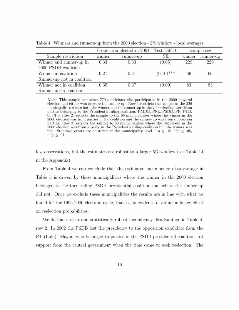
Table 4: Winners and runners-up from the 2000 election - 2% window - local averages
Proportion elected in 2004 Test Diff=0 sample sizeSample restriction winner runner-up SE winner runner-up
Winner and runner-up in 0.33 0.33 (0.05) 229 2292000 PSDB coalitionWinner in coalition 0.21 0.51 (0.10)*** 66 66Runner-up not in coalitionWinner not in coalition 0.35 0.37 (0.09) 83 83Runner-up in coalition
Note: This sample comprises 770 politicians who participated in the 2000 mayoralelection and either won or were the runner up. Row 1 restricts the sample to the 229municipalities where both the winner and the runner-up in the 2000 election were fromparties belonging to the President’s ruling coalition: PMDB, PFL, PSDB, PP, PTB,or PPS. Row 2 restricts the sample to the 66 municipalities where the winner in the2000 election was from parties in the coalition and the runner-up was from oppositionparties. Row 3 restricts the sample to 83 municipalities where the runner-up in the2000 election was from a party in the President’s ruling coalition but the winner wasnot. Standard errors are clustered at the municipality level. ∗
p ≤ .10, ∗∗p ≤ .05,
∗∗∗p ≤ .01.
few observations, but the estimates are robust to a larger 5% window (see Table 14
in the Appendix).
From Table 4 we can conclude that the estimated incumbency disadvantage in
Table 5 is driven by those municipalities where the winner in the 2000 election
belonged to the then ruling PSDB presidential coalition and where the runner-up
did not. Once we exclude these municipalities the results are in line with what we
found for the 1996-2000 electoral cycle, that is, no evidence of an incumbency effect
on reelection probabilities.
We do find a clear and statistically robust incumbency disadvantage in Table 4,
row 2. In 2002 the PSDB lost the presidency to the opposition candidate from the
PT (Lula). Mayors who belonged to parties in the PSDB presidential coalition lost
support from the central government when the time came to seek reelection. The
16

new presidential coalition led by the PT may have been able to influence these close
elections through mechanisms such as coattail effects from Lula’s popularity or the
lost capacity for the parties in the PSDB coalition to raise campaign money. The
clearest mechanism, however, seems to be the one suggested by Brollo and Nannicini
(2010). Their evidence suggests that the federal government is able to starve of funds
the municipalities where the incumbent belongs to the opposition.
The largest share of the municipal budget is made of federal transfers (65% on
average). The remaining is divided between state funds (30%) and locally raised
revenues from property taxes, fines, as service taxes (5%). A small share of federal
transfers are discretionary (the largest share is linked to population variables and
total national tax revenue). The discretionary transfers consist of amendments to
the federal budget proposed by legislators. The President is not required by law
to implement the approved amendments. Brollo and Nannicini (2010) show that
mayors who do not belong to a party in the presidential coalition are less likely to
receive discretionary funds from the central government.
The results in Table 4 suggest that the mechanism described in Brollo and Nannicini
(2010) may play an important part in explaining the incumbency effects in the 2000-
2004 electoral cycle. We only observe signs of an incumbency disadvantage in the
municipalities where incumbent mayors belonged to parties in the opposition (row
2). We observe no incumbency advantage where the incumbents belonged to the rul-
ing coalition (row 3). Had the other mechanisms I mentioned, coattail effects from
Lula’s popularity and difficulty in raising campaign funds, played an important role
we would have expected a positive incumbency effect in row 3.
THE 2004-2008 ELECTORAL CYCLE
In Table 5 I present the results for the 2004-2008 electoral cycle. In contrast to the
17

results of both previous cycles we observe a clear incumbency advantage. In row 1
we can see that around 41% of winners in the 2004 election are reelected in 2008
whereas only 27% or runners-up are elected mayor in 2008. This results is statistically
significant and is robust to the polynomial method as we can see in Table 16 in the
Appendix. Rows 2 to 8 again reassure us that we can interpret close elections in
this sample as quasi-experiments. In row 6 we can seen that the average campaign
expenditure among incumbents is not statistically different to the expenditure by
the runners-up in 2004. These results are also robust to the polynomial method (see
the Appendix Table 17).
Table 5: Winners and runners-up from the 2004 election - 2% window - local averages
mean Test Diff=0 sample sizewinner runner-up SE winner runner-up
Elected Mayor in 2008 0.41 0.27 (0.04)*** 488 488Education 0.72 0.73 (0.03) 447 445Married 1.00 1.01 (0.03) 445 443Age 47.3 47.8 (0.63) 446 447Gender 0.06 0.07 (0.02) 446 445Declared campaign cost 182,615 197,911 (23,925) 448 448President’s party (PT) 0.07 0.09 (0.02) 448 448President’s Coalition 0.48 0.49 (0.04) 448 448Ran for Mayor in 2008 0.70 0.53 (0.03)*** 448 448Ran in 2008(mayor, ver., d-m) 0.71 0.67 (0.03) 448 448Party Switch in 2008 0.28 0.34 (0.03)* 319 302Diff in Vote(%) 04-08 4.80 -0.20 (1.46)*** 313 237Prob(win 08| running) 0.59 0.50 (0.05)* 313 237
Note: This sample comprises 896 politicians who participated in the 2000 mayoralelection and either won or were the runner up. The sample consists of 488 munici-palities where a two-year term limit for mayors was not binding. Standard errors areclustered at the municipality level. ∗
p ≤ .10, ∗∗p ≤ .05, ∗∗∗
p ≤ .01.
The results in row 9 and 10 are similar to those for the 1996-2000 cycle. Incum-
18
bents are more likely to run for mayor, but runners-up are as likely to run again in the
next local election as incumbents. The difference is that runners-up are more likely
to run for either local council or as deputy-mayor. In the 1996-2000 cycle around
60% of candidates for mayors in close elections chose to run again. In the 2004-2008
cycle this average is higher: 70%. The result in row 11 is similar to all other electoral
cycles: runners-up are slightly more likely to switch parties (conditional on running)
than incumbents.
There is a stark difference between the results in rows 12 and 13 in Table 5 and the
results in the previous electoral cycles. In the 2004-2008 electoral cycle, conditional
on running, incumbents increase their votes share whereas the runners-up see little
change in theirs. Moreover, the probability of winning conditional on running is
higher for incumbents than for runners-up.
In Table 6 we can see that the incumbency advantage is found in every type of
race. In particular, there is an incumbency advantage even in the races where the
incumbent mayor belonged to the opposition and the runner-up belonged to a party
in the presidential ruling coalition led by the PT (row 3). The presidential coalition
led by the PT included the following parties: PMDB, PT, PSB, PDT, PL, PTB,
PV, and PC do B.
The mechanism suggested by Brollo and Nannicini (2010), which looks like a
good candidate to explain the results in the 2000-2004 electoral cycle, seems to
have little effect in the 2004-2008 electoral cycle. This may not be surprising as the
mayors elected in 2004 were already under a federal government led by the PT. Their
candidacy and vote share in 2004 were conditional on the President being Lula from
the PT.
Two other potential mechanisms to explain the incumbency advantage found in
the 2004-2008 electoral cycle may be Lula’s high popularity and/or the highest level
19

Table 6: Winners and runners-up from the 2004 election - 2% window - local averages
Proportion elected in 2004 Test Diff=0 sample sizeSample restriction winner runner-up SE winner runner-up
Winner and runner-up in 0.44 0.19 (0.08)*** 86 86President’s coalitionWinner in coalition 0.43 0.27 (0.07)** 130 130Runner-up not in coalitionWinner not coalition 0.41 0.28 (0.07)* 133 133Runner-up in coalition
Note: This sample comprises 976 politicians who participated in the 2004 mayoralelection and either won or were the runner up. Row 1 restricts the sample to the86 municipalities where both the winner and the runner-up in the 2004 election werefrom parties belonging to the President’s ruling coalition: PT, PMDB, PSB, PDT,PL, PTB, PV, PC do B. Row 2 restricts the sample to the 130 municipalities wherethe winner in the 2004 election was from parties in the coalition and the runner-upwas from parties in the opposition. Row 3 restricts the sample to 133 municipalitieswhere the winner was not from a party in the President’s coalition and the runner-upwas from a party in the President’s coalition. Standard errors are clustered at themunicipality level. ∗
p ≤ .10, ∗∗p ≤ .05, ∗∗∗
p ≤ .01.
of economic growth since the 70’s. Economic growth has not only an impact on job
creation and other direct effects, but also on tax revenues. And as the tax revenue
grows, so does the amount that is transferred to municipalities from the central
government. Most of the transferred amount is constitutionally mandated as a share
of total revenues. So mayors that serve through a period on increasing national tax
revenues will see their budget increase regardless of the policies they implement at
the municipality level. The evidence in Sakurai and Menezes-Filho (2008), supports
this interpretation. Their findings suggest that mayors who spend more during their
term in office increase their probability of reelection.
DISCUSSION
Brazilian mayors have little power to raise revenue on their own (on average 5%
20
of revenues are locally raised). The largest share of the municipal budget is made
of federal transfers (65% on average). The constitution mandates that a share of
national revenue be transferred to municipalities. If the economy grows nationally
all municipalities benefit from higher transfers. The results I presented here suggest
that the ability of mayors to be reelected depends on how the Brazilian economy
fares (as suggested by the results for the 2004-2008 electoral cycle), and on how
mayors are connected to the central government (as suggested by the results in the
2000-2004 electoral cycle). The evidence in Ames (1994) suggests that mayors are
able to influence the presidential vote in their municipality. One would only expect
that the central government would try and influence local politics as well.
Other potential mechanisms that may explain incumbency effects on reelection
probabilities are popularity coattail effects, the funneling of state funds for electoral
purposes, media control (see Boas and Hidalgo (2011)), and so on. Identifying what
other mechanisms have an impact on incumbency effects is an important avenue for
future research.
The results presented here are also a contribution to the study of political careers
in Brazil. We’ve seen that no more than 4% of candidates for mayors go on to a
state or federal office. We’ve also seen that around 60 to 70% of politicians who
run for mayor will be present in the next local election whether they win or lose.
Those who become mayors will run for reelection, those that lost may either run for
mayor again, or for the local council, or as deputy-mayor. Finally, we’ve seen that
around 30% of politicians who run for mayor again switch parties before the next
local elections. Candidates who become mayors are slightly less likely to switch than
runners-up.
The best summary for the results regarding the 1996-2000 electoral cycle is that
close elections are close elections. Mayors have little direct control over the size of
21

their budget. The same President and coalition stayed in power. The President was
moderately popular and governed during a period of moderate economic growth.
Without major changes at the federal level between 1996 and 2000 it is only normal
to expect that both incumbents and runners-up in close elections in 1996 would have
similar chances of being elected in 2000.
During the 2000-2004 electoral cycle there is a major political change. The PSDB
loses the presidency to the PT. President Lula takes power in January 2003. This
political change may explain the incumbency disadvantage in municipalities where
the incumbent belonged to the opposition (a party in the PSDB coalition) and the
runner-up belonged to the PT coalition that came to power in 2002. A possible
mechanism through which the central government may have been able to influence
the 2004 local elections was proposed by Brollo and Nannicini (2010). Their results
suggest that the central government is able to starve of funds the municipalities that
are held by mayors who belong to the opposition. Our results for the 2000-2004
electoral cycle support this interpretation because we only observe an incumbency
disadvantage in the municipalities where the incumbents belonged to the opposition
and the runners-up belonged to the presidential coalition. We observe no incumbency
advantage in the sample of municipalities where the incumbents belonged to the
presidential coalition and the runners-up belonged to the opposition.
In the 2004 and 2008 cycle there is a clear incumbency advantage throughout,
even where the incumbent belonged to the opposition and the runner-up belonged
to the ruling coalition. The mechanism of starving of funds the municipalities in
the hands of the opposition seems to have little effect in the 2004-2008 electoral
cycle. A possible mechanism to explain the incumbency advantage in 2008 was the
rapid economic growth during the period coupled with its effect of increasing central
government revenue, which automatically increases central government transfers to
22

all municipalities.
23

References
Ames, B. (1994). The reverse coattails effect: Local party organization in the 1989
brazilian presidential election. The American Political Science Review, 88(1):95–
111.
Ansolabehere, S., Snyder, J., and Stewart, C. (2000). Old voters, new voters, and the
personal vote: Using redistricting to measure the incumbency advantage. Ameri-
can Journal of Political Science, 44(1):17–34.
Boas, T. C. and Hidalgo, F. D. (2011). Controlling the airwaves: Incumbency ad-
vantage and community radio in brazil. American Journal of Political Science,
55(4):868–884.
Brambor, T. and Ceneviva, R. (2011). Incumbency advantage in brazilian mayoral
elections. Working Paper.
Brollo, F. and Nannicini, T. (2010). Tying your enemy’s hands in close races: The
politics of federal transfers in brazil. Working Paper.
Brollo, F., Nannicini, T., Perotti, R., and Tabellini, G. (2010). The political resource
curse. NBER Working Paper 15705.
Carey, J. M., Niemi, R. G., and Powell, L. W. (2000). Incumbency and the probability
of reelection in state legislative elections. Journal of Politics, 62(3):671700.
Caughey, D. M. and Sekhon, J. S. (2012). Elections and the regression-discontinuity
design: Lessons from u.s. house races, 1942-2008. Political Analysis.
Collie, M. (1981). Incumbency, electoral safety, and turnover in the house of repre-
sentatives. The American Political Science Review, 75(1):119–131.
24

Cox, G. W. and Katz, J. N. (1996). Why did the incumbency advantage in u.s. house
elections grow? American Journal of Political Science, 40(2):478–497.
Desposato, S. W. (2006). Parties for rent? ambition, ideology, and party switching in
brazil’s chamber of deputies. American Journal of Political Science, 50(1):62–80.
Ferejohn, J. A. (1977). On the decline of competition in congressional elections. The
American Political Science Review, 71(1):166–176.
Ferraz, C. and Finan, F. (2008). Exposing corrupt politicians: The effects of brazil’s
publicly released audits on electoral outcomes. Quarterly Journal of Economics.
Ferraz, C. and Finan, F. (2011). Electoral accountability and corruption: Evidence
from the audits of local governments. American Economic Review, 101:12741311.
Ferreira, F. and Gyourko, J. (2009). Do political parties matter? evidence from u.s.
cities. The Quarterly Journal of Economics, 124(1):399–422.
Gordon, S. C., Huber, G. A., and Landa, D. (2007). Challenger entry and voter
learning. American Political Science Review, 101(2):303–320.
Hahn, J., Todd, P., and Van der Klaauw, W. (2001). Identification and estimation of
treatment effects with a degression-discontinuity design. Econometrica, 69(1):201–
209.
Lee, D. S. (2008). Randomized experiments from non-random selection in u.s. house
elections. Journal of Econometrics, 142:675–697.
Lee, D. S. and Lemieux, T. (2009). Regression discontinuity design in economics.
NBER Working Paper 14723.
25

Miguel, E. and Zaidi, F. (2003). Do politicians reward their supporters? regression
discontinuity evidence from ghana. Working Paper.
Sakurai, S. and Menezes-Filho, N. (2008). Fiscal policy and reelection in brazilian
municipalities. Public Choice, 137(1):301–314.
Samuel, D. J. (2002). Pork barreling is not credit claiming or advertising: Campaign
finance and the sources of the personal vote in brazil. The Journal of Politics,
64(03):845–863.
Titiunik, R. (2009). Incumbency advantage in brazil: Evidence from municipal mayor
elections. Working Paper.
Uppal, Y. (2008). The disadvantaged incumbents: estimating incumbency effects in
indian state legislatures. Public Choice, 138(1-2):9–27.
26

A APPENDIX
Table 7: Winners and runners-up from the 1996 election - Summary Statistics - Allsample
mean Test Diff=0 sample sizewinner runner-up SE winner runner-up
Elected Mayor in 2000 0.36 0.15 (0.01)*** 5374 5221Education 0.63 0.61 (0.01)* 3637 3517Married 0.98 0.99 (0.01) 3621 3500Age 46.3 46.8 (0.20)** 4762 4439Gender 0.05 0.06 (0.00)** 3651 3533President’s party(PSDB) 0.17 0.14 (0.01)*** 5374 5221President’s Coalition 0.78 0.76 (0.01)** 5374 5221Ran for Mayor in 2000 0.64 0.30 (0.01)*** 5374 5221Ran in 2000(mayor, ver., d-m) 0.64 0.50 (0.01)*** 5374 5221Won 98-02-06 (state or national) 0.03 0.03 (0.00) 5374 5221Party Switch in 2000 0.29 0.37 (0.01)*** 3431 2616Diff in Vote(%) 00-96 -4.61 3.60 (0.45)*** 3402 1576Prob(win 00| running) 0.58 0.49 (0.02)*** 3402 1576
Note: This sample comprises 10598 politicians who participated in the 1996 mayoralelection and either won or were the runner up. Standard errors are clustered at themunicipality level. ∗
p ≤ .10, ∗∗p ≤ .05, ∗∗∗
p ≤ .01.
27

Table 8: Election probabilities regressed on vote share - 1996-2000 - Polynomials
Method Jump at 50% SE3-degree polynomials 0.01 (0.02)4-degree polynomials -0.00 (0.03)5-degree polynomials -0.01 (0.03)6-degree polynomials -0.00 (0.04)
Note: This sample comprises 10430 politicians who participated in the 1996 mayoralelection and either won or were the runner up. The dependent variable takes value 1 ifthe politician ran for reelection in 2000 and won, and takes the value 0 if the politiciandid not run or ran and lost in the 2000 election. The forcing variable is Vote margin- the difference of votes in percentage terms between the winner and the runner up.The discontinuity is estimated at Vote margin = 0. Row 1 shows the results for a3-degree polynomial on each side of the cutoff. Row 2 to 4 shows the results for a4-degree polynomial, a 5-degree polynomial, and a 6 degree polynomial respectively.Standard errors are clustered at the municipality level. ∗
p ≤ .10, ∗∗p ≤ .05, ∗∗∗p ≤ .01
.
Table 9: Balance test for Mayors elected in 1996 - Polynomial (4)
Method Jump at 50% SE No. ObservationsElected Mayor in 2000 -0.00 (0.03) 10444Education 0.02 (0.03) 7046Married 0.03 (0.03) 7014Age -0.24 (0.57) 9075Gender 0.03 (0.01)** 7076President’s party(PSDB) 0.01 (0.02) 10444President’s Coalition 0.00 (0.02) 10444Ran for Mayor in 2000 0.15 (0.03)*** 10444Ran in 2000(mayor, ver., d-m) 0.00 (0.03) 10444Won 98-02-06 (state or national) -0.01 (0.01) 10444Party Switch in 2000 -0.08 (0.03)** 5984Diff in Vote(%) 00-96 -1.42 (1.15) 4915Prob(win 00| running) -0.14 (0.05)*** 4915
Note: This sample comprises 10444 politicians who participated in the 1996 mayoralelection and either won or were the runner up. The forcing variable is Vote margin- the difference of votes in percentage terms between the winner and the runner up.The discontinuity is estimated at Vote margin = 0 with a 4-degree polynomial on eachside of the cutoff. Standard errors are clustered at the municipality level. ∗
p ≤ .10,∗∗p ≤ .05, ∗∗∗
p ≤ .01.
28

Table 10: Winners and runners-up from the 1996 election - 5% window
mean Test Diff=0 sample sizewinner runner-up SE winner runner-up
Elected Mayor in 2000 0.31 0.24 (0.02)*** 1345 1345Education 0.63 0.61 (0.02) 945 943Married 0.99 0.97 (0.02) 940 939Age 45.4 45.8 (0.46) 945 946Gender 0.05 0.04 (0.01) 948 949President’s party(PSDB) 0.16 0.13 (0.01)* 1345 1345President’s Coalition 0.76 0.76 (0.02) 1345 1345Ran for Mayor in 2000 0.63 0.42 (0.02)*** 1345 1345Ran in 2000(mayor, ver., d-m) 0.63 0.58 (0.02)*** 1345 1345Won 98-02-06 (state or national) 0.03 0.03 (0.01) 1345 1345Party Switch in 2000 0.27 0.35 (0.02)*** 848 782Diff in Vote(%) 00-96 -0.00 2.47 (0.76)*** 837 567Prob(win 00| running) 0.49 0.57 (0.03)** 837 567
Note: This sample comprises 2690 politicians who participated in the 1996 mayoralelection and either won or were the runner up. Standard errors are clustered at themunicipality level. ∗
p ≤ .10, ∗∗p ≤ .05, ∗∗∗
p ≤ .01.
29
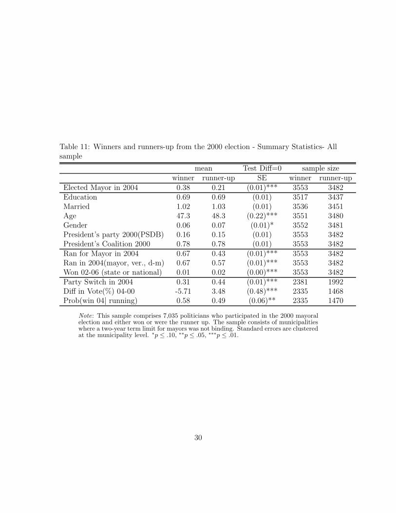
Table 11: Winners and runners-up from the 2000 election - Summary Statistics- Allsample
mean Test Diff=0 sample sizewinner runner-up SE winner runner-up
Elected Mayor in 2004 0.38 0.21 (0.01)*** 3553 3482Education 0.69 0.69 (0.01) 3517 3437Married 1.02 1.03 (0.01) 3536 3451Age 47.3 48.3 (0.22)*** 3551 3480Gender 0.06 0.07 (0.01)* 3552 3481President’s party 2000(PSDB) 0.16 0.15 (0.01) 3553 3482President’s Coalition 2000 0.78 0.78 (0.01) 3553 3482Ran for Mayor in 2004 0.67 0.43 (0.01)*** 3553 3482Ran in 2004(mayor, ver., d-m) 0.67 0.57 (0.01)*** 3553 3482Won 02-06 (state or national) 0.01 0.02 (0.00)*** 3553 3482Party Switch in 2004 0.31 0.44 (0.01)*** 2381 1992Diff in Vote(%) 04-00 -5.71 3.48 (0.48)*** 2335 1468Prob(win 04| running) 0.58 0.49 (0.06)** 2335 1470
Note: This sample comprises 7,035 politicians who participated in the 2000 mayoralelection and either won or were the runner up. The sample consists of municipalitieswhere a two-year term limit for mayors was not binding. Standard errors are clusteredat the municipality level. ∗
p ≤ .10, ∗∗p ≤ .05, ∗∗∗
p ≤ .01.
30

Table 12: Election probabilities regressed on vote share - 2000-2004 - Polynomials
Method Jump at 50% SE3-degree polynomials -0.08 (0.03)**4-degree polynomials -0.09 (0.04)**5-degree polynomials -0.09 (0.04)**6-degree polynomials -0.08 (0.05)*
Note: This sample comprises 6964 politicians who participated in the 2000 mayoralelection and either won or were the runner up. This samples does not include munic-ipalities where the incumbent Mayor in 2004 faced a two-term limit. The dependentvariable takes value 1 if the politician ran for reelection in 2004 and won, and takesthe value 0 if the politician did not run or ran and lost in the 2004 election. Theforcing variable is Vote margin - the difference of votes in percentage terms betweenthe winner and the runner up. The discontinuity is estimated at Vote margin = 0.Row 1 shows the results for a 3-degree polynomial on each side of the cutoff. Row 2to 4 shows the results for a 4-degree polynomial, a 5-degree polynomial, and a 6 de-gree polynomial respectively. Standard errors are clustered at the municipality level.∗p ≤ .10, ∗∗
p ≤ .05, ∗∗∗p ≤ .01.
31

Table 13: Balance test for Mayors elected in 2000 - Polynomial (4)
Method Jump at 50% SE No. ObservationsElected Mayor in 2004 -0.09 (0.04)** 6964Education -0.02 (0.03) 6884Married 0.04 (0.03) 6916Age 1.46 (0.64)** 6960Gender 0.00 (0.02) 6962Presidents’s party 2000(PSDB) -0.03 (0.03) 6964Presidents’s Coalition in 2000 -0.03 (0.03) 6964Ran for Mayor in 2004 0.03 (0.03) 6964Ran in 2004(mayor, ver., d-m) -0.05 (0.03) 6964Won 02-06 (state or national) -0.03 (0.01)*** 6964Party Switch in 2004 -0.07 (0.04)* 4328Diff in Vote(%) 04-00 -2.48 (1.16)** 3759Prob(win 04| running) -0.18 (0.05)*** 3761
Note: This sample comprises 6964 politicians who participated in the 2000 mayoralelection and either won or were the runner up. This samples does not include mu-nicipalities where the incumbent Mayor in 2004 faced a two-term limit. The forcingvariable is Vote margin - the difference of votes in percentage terms between the win-ner and the runner up. The discontinuity is estimated at Vote margin = 0 with a4-degree polynomial on each side of the cutoff. Standard errors are clustered at themunicipality level. ∗
p ≤ .10, ∗∗p ≤ .05, ∗∗∗
p ≤ .01.
32

Table 14: Winners and runners-up from the 2000 election - 5% window - local aver-ages
Proportion elected in 2004 Test Diff=0 sample sizeSample restriction winner runner-up SE winner runner-up
Winner and runner-up in 0.30 0.31 (0.03) 546 5462000 PSDB coalitionWinner in coalition 0.28 0.40 (0.06)* 161 161Runner-up not in coalitionWinner not in coalition 0.33 0.31 (0.06) 185 185Runner-up in coalition
Note: This sample comprises 770 politicians who participated in the 2000 mayoralelection and either won or were the runner up. Standard errors are clustered at themunicipality level. ∗
p ≤ .10, ∗∗p ≤ .05, ∗∗∗
p ≤ .01.Row 1 restricts the sample to the229 municipalities where both the winner and the runner-up in the 2000 election werefrom parties belonging to the President’s ruling coalition: PMDB, PFL, PSDB, PP,PTB, or PPS. Row 2 restricts the sample to the 66 municipalities where the winnerin the 2000 election was from parties in the coalition and the runner-up was fromopposition parties. Row 3 restricts the sample to 83 municipalities where the runner-up in the 2000 election was from a party in the President’s ruling coalition but thewinner was not.
33

Table 15: Winners and runners-up from the 2004 election - Summary Statistics - Allsample
mean Test Diff=0 sample sizewinner runner-up SE winner runner-up
Elected Mayor in 2008 0.51 0.13 (0.01)*** 4128 4042Education 0.74 0.72 (0.01)*** 4094 4001Married 0.99 1.01 (0.01) 4093 4012Age 46.4 47.8 (0.21)*** 4093 4123Gender 0.08 0.10 (0.01)*** 4099 4019Declared campaign cost 202,566 193,342 (9,867) 4128 4042President’s party (PT) 0.08 0.08 (0.01) 4128 4042President’s Coalition 0.52 0.52 (0.01) 4128 4042Ran for Mayor in 2008 0.76 0.34 (0.01)*** 4128 4042Ran in 2008(mayor, ver., v-m) 0.76 0.53 (0.01)*** 4128 4042Party Switch in 2008 0.31 0.39 (0.01)*** 3149 2153Diff in Vote(%) 04-08 -0.74 0.15 (0.60)*** 3125 1353Prob(win 08| running) 0.67 0.40 (0.01)*** 3122 1352
Note: This sample comprises 8,170 politicians who participated in the 2000 mayoralelection and either won or were the runner up. The sample consists of municipalitieswhere a two-year term limit for mayors was not binding. Standard errors are clusteredat the municipality level. ∗
p ≤ .10, ∗∗p ≤ .05, ∗∗∗
p ≤ .01.
34

Table 16: Election probabilities regressed on vote share - 2004-2008 - Polynomials
Method Jump at 50% SE3-degree polynomials 0.13 (0.03)***4-degree polynomials 0.10 (0.03)***5-degree polynomials 0.09 (0.04)**6-degree polynomials 0.08 (0.04)*
Note: This sample comprises 8092 politicians who participated in the 2004 mayoralelection and either won or were the runner up. This samples does not include munic-ipalities where the incumbent Mayor faced a two-term limit in 2008 . The dependentvariable takes value 1 if the politician ran for reelection in 2008 and won, and takesthe value 0 if the politician did not run or ran and lost in the 2008 election. Theforcing variable is Vote margin - the difference of votes in percentage terms betweenthe winner and the runner up. The discontinuity is estimated at Vote margin = 0.Row 1 shows the results for a 3-degree polynomial on each side of the cutoff. Row 2to 4 shows the results for a 4-degree polynomial, a 5-degree polynomial, and a 6 de-gree polynomial respectively. Standard errors are clustered at the municipality level.∗p ≤ .10, ∗∗
p ≤ .05, ∗∗∗p ≤ .01.
35

Table 17: Balance test for Mayors elected in 2004 - Polynomial (4)
Method Jump at 50% SE No. ObservationsElected Mayor in 2008 0.10 (0.03)*** 8092Education 0.00 (0.02) 8017Married -0.15 (0.03) 8027Age 0.28 (0.56) 8084Gender 0.00 (0.02) 8040Declared campaign cost -7,430 (23,510) 8092President’s Party (PT) 0.01 (0.02) 8092President’s Coalition -0.01 (0.03) 8092Ran for Mayor in 2008 0.17 (0.03)*** 8092Ran in 2008(mayor, ver., d-m) 0.04 (0.03) 8092Party Switch in 2008 -0.06 (0.03)* 5243Diff in Vote(%) 04-08 3.06 (1.40)** 4420Prob(win 08| running) -0.00 (0.05) 4416
Note: Total sample 8090; This sample comprises 8092 politicians who participatedin the 2004 mayoral election and either won or were the runner up. This samplesdoes not include municipalities where the incumbent Mayor faced a two-term limitin 2008. The forcing variable is Vote margin - the difference of votes in percentageterms between the winner and the runner up. The discontinuity is estimated at Votemargin = 0 with a 4-degree polynomial on each side of the cutoff. Standard errors areclustered at the municipality level. Standard errors are clustered at the municipalitylevel. ∗
p ≤ .10, ∗∗p ≤ .05, ∗∗∗
p ≤ .01.
36