Embed Size (px)
Citation preview

Page 1
IncuCyte™ ZOOM Users Manual
2013A
Essen BioScience, Inc.
www.EssenBioScience.com

Page 2
Table of Contents IncuCyte™ ZOOM Users Manual .................................................................................................................... 1
2013A .............................................................................................................................................................. 1
Chapter 1: Warranty ................................................................................................................................. 5
1.1 Limitation of Warranty .................................................................................................................... 5
1.2 Exclusive Remedies ......................................................................................................................... 5
1.3 Warnings and Disclaimers ............................................................................................................... 5
Chapter 2: Getting to know your IncuCyte™ ZOOM ....................................................................................... 6
2.1 Intended Use ................................................................................................................................... 6
2.2 IncuCyte™ ZOOM Configurations ................................................................................................... 6
2.3 Safety has Priority ........................................................................................................................... 6
2.4 IncuCyte™ ZOOM Specifications ..................................................................................................... 7
2.5 Unpacking and Checking the IncuCyte™ ......................................................................................... 8
Chapter 3: Installation of the IncuCyte™ ZOOM Hardware .......................................................................... 10
3.1 IncuCyte™ ZOOM Hardware Features .......................................................................................... 10
3.2 Removing the Shipping Pin ........................................................................................................... 12
3.3 Installing the Filter Module ........................................................................................................... 13
3.4 Installing an Objective ................................................................................................................... 14
3.5 Positioning the Controller ............................................................................................................. 14
3.6 Placing the Microscope into the Incubator ................................................................................... 15
3.7 Switching the IncuCyte™ ZOOM On and Off ................................................................................. 16
3.8 Warming up the Microscope ........................................................................................................ 16
3.8.1 Auto Warm-up ...................................................................................................................... 17
3.8.2 IncuCyte™ Controller Air Filter .............................................................................................. 17
Chapter 4: Establishing Network Connections ....................................................................................... 18
4.1 DHCP Based Networks .................................................................................................................. 18
4.1.1 Verifying the IncuCyte™ Controller Network Connection: Windows Vista or Windows 7 ... 19
4.1.2 Verifying the IncuCyte™ Controller Network Connection: Windows XP .............................. 19
4.2 Static IP Based Networks .............................................................................................................. 20
Chapter 5: Installation of the IncuCyte™ Control Software .................................................................... 20

Page 3
5.1 IncuCyte™ Control Software Installation using Windows XP ........................................................ 20
5.2 IncuCyte™ Control Software Installation using Windows Vista and Windows 7 .......................... 21
5.3 Connecting .................................................................................................................................... 21
5.3.1 Setting the Date and Time .................................................................................................... 21
5.3.2 Establishing User Accounts ................................................................................................... 22
5.4 Remote Administration of the Controller ..................................................................................... 23
Chapter 6: Calibrating the IncuCyte™ ZOOM System ............................................................................. 24
6.1 System Calibration ........................................................................................................................ 24
6.2 Fluorescence Calibration ............................................................................................................... 26
6.2.1 FLR Calibration Results .......................................................................................................... 27
Chapter 7: Cell Culture Monitoring and Data Analysis ........................................................................... 27
7.1 Introduction .................................................................................................................................. 27
7.2 User Interface ............................................................................................................................... 28
7.3 Scheduling Scans and Loading Vessels .......................................................................................... 29
7.3.1 24-Hour Repeating ................................................................................................................ 29
7.3.2 Scan on Demand ................................................................................................................... 34
7.4 Finding and Viewing Scanned Vessels ........................................................................................... 35
7.4.1 Finding Scanned Vessels ....................................................................................................... 35
7.4.2 Vessel View ........................................................................................................................... 37
7.5 Data Processing ............................................................................................................................. 40
7.5.1 Assay Mode vs. Established Mode ........................................................................................ 40
7.5.2 Analysis Job Utilities .............................................................................................................. 41
7.6 Graphing and Exporting Data ........................................................................................................ 47
7.6.1 Create a Graph ...................................................................................................................... 47
7.6.2 Microplate Graphing ............................................................................................................. 61
7.6.3 Exporting Experimental Data ................................................................................................ 62
7.6.4 Saving and Printing Graphs ................................................................................................... 66
7.7 Exporting Images and Movies ....................................................................................................... 66
7.7.1 Exporting Images Overview .................................................................................................. 66
7.7.2 Exporting Movies Overview .................................................................................................. 72

Page 4
7.8 Archiving ....................................................................................................................................... 74
7.8.1 Archiving Vessels ................................................................................................................... 75
7.8.2 Opening an Archive ............................................................................................................... 76
7.9 Hardware ...................................................................................................................................... 77
7.9.1 Selecting and Placing Trays ................................................................................................... 77
7.9.2 Changing Objectives .............................................................................................................. 79
7.10 Plate Map Editor ........................................................................................................................... 81
7.10.1 Selecting Wells ...................................................................................................................... 82
7.10.2 Adding Well Items ................................................................................................................. 82
Chapter 8: Special Modules and Scan Types .......................................................................................... 85
8.1 Scan Types available with Essen ImageLock™ .............................................................................. 85
8.1.1 Standard (with Lock) ............................................................................................................. 85
8.1.2 Scratch Wound ...................................................................................................................... 85
8.2 Cell Migration/Invasion Module ................................................................................................... 86
8.3 Angiogenesis Analysis Module ...................................................................................................... 86
8.3.1 Tiled Field of View Mosaic Imaging Mode ................................................................................... 86
8.4 NeuroTrackTM Module ................................................................................................................... 87
Chapter 9: Troubleshooting .................................................................................................................... 88
9.1 Images and What they Mean ........................................................................................................ 89
9.2 Contacting Technical Support ....................................................................................................... 92
Chapter 10: Performance Optimization .................................................................................................... 93

Page 5
NO OTHER WARRANTY IS EXPRESED OR IMPLIED. ESSEN BIOSCIENCE INC SPECIFICALLY DISCLAIMS THE IMPLIED WARRANTIES OR MERCHANTABILITY AND FITNESS FOR A PARTICULAR PURPOSE.
THE REMEDIES PROVIDED HEREIN ARE BUYER’S SOLE AND EXCLUSIVE REMEDIES. ESSEN BIOSCIENCE INC. SHALL NOT BE LIABLE FOR ANY DIRECT, INDIRECT, SPECIAL, INCIDENTAL, OR CONSEQUENTIAL
DAMAGES, WHETHER BASED ON CONTRACT, TORT, OR ANY OTHER LEGAL THEORY.
Chapter 1: Warranty Your Essen BioScience Inc. (Essen) IncuCyte™ product is warranted against defects in material and workmanship for a period of one year following delivery to the Buyer. Essen warrants to its original Buyer only. The Buyer must notify Essen in writing within fifteen (15) days following discovery of the defect. During the warranty period, Essen will, at its option, either repair or replace products that prove to be defective.
For warranty service or repair, this product must be returned to the Essen factory. Buyer shall prepay shipping charges to Essen, and Essen shall pay shipping charges to return the product to the Buyer. However, Buyer shall pay all shipping charges, duties and taxes for products returned to Essen from another country.
1.1 Limitation of Warranty The foregoing warranty shall not apply to defects resulting from improper or inadequate maintenance by Buyer, Buyer-supplied software or interfacing, unauthorized modification, misuse, or operation outside of the environmental specifications.
1.2 Exclusive Remedies
1.3 Warnings and Disclaimers Doing any of the following may void your warranty:
WARNING: DO NOT RUN THE STERILIZATION CYCLE ON AN INCUBATOR WITH THE INCUCYTETM ZOOM GANTRY INSIDE.
WARNING: DO NOT TURN OFF THE INCUCYTETM ZOOM AND LEAVE THE GANTRY INSIDE THE
INCUBATOR. CONDENSATION BUILDUP CAN DAMAGE THE ELECTRONICS.
Essen BioScience is not responsible for data loss due to hardware failure.

Page 6
Chapter 2: Getting to know your IncuCyte™ ZOOM
2.1 Intended Use The IncuCyte™ ZOOM is intended to facilitate live-cell monitoring via customized imaging protocols. It is intended for experimental purposes only. Please read carefully through the operating instructions in this manual to ensure that you can properly and safely utilize all features of your new instrument.
2.2 IncuCyte™ ZOOM Configurations The IncuCyte™ ZOOM is user configurable through the installation of objectives (4X, 10X, 20X),
filter modules, and software modules. The use of fluorescence filter modules and application
specific software modules requires the user to purchase a license. This will be indicated in the
manual where applicable.
Current Filter modules available are:
#4460 IncuCyte ZOOM HD Filter Cube (High Definition Phase Contrast only)
#4459 IncuCyte ZOOM HD/Dual Color Filter Cube (High Definition Phase Contrast, Green and
Red Fluorescence)
2.3 Safety has Priority Please note the following directions for safe and problem-free operation of your IncuCyte™ ZOOM. Read through these operating instructions carefully.
It is essential to follow the instructions in Section 3, page 10 when putting your new IncuCyte™ ZOOM into operation.
The unit must only be connected to a receptacle-outlet with a grounding connection.
Use only the AC power cord supplied or an equivalent cord with an IEC-320-C13 standard connector approved for operation at 5 amps and the appropriate voltage for your local power. Also, ensure the local line voltage falls within the range printed on the IncuCyte ZOOM Controller.
NEVER open the IncuCyte™ ZOOM controller. It does not contain any parts that need to be maintained, repaired or changed by the User.
If the IncuCyte™ ZOOM is not used in the manner as described in this manual, provided protections may be impaired.
Page 7
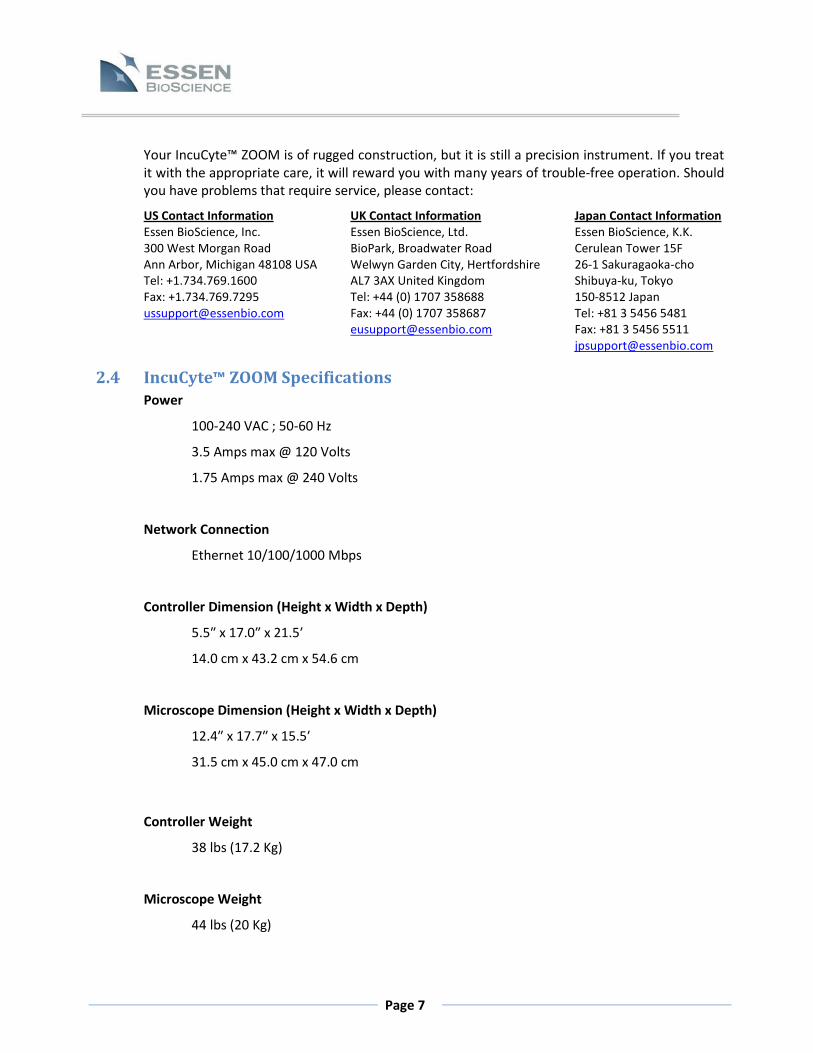
Your IncuCyte™ ZOOM is of rugged construction, but it is still a precision instrument. If you treat it with the appropriate care, it will reward you with many years of trouble-free operation. Should you have problems that require service, please contact:
US Contact Information UK Contact Information Japan Contact Information Essen BioScience, Inc. Essen BioScience, Ltd. Essen BioScience, K.K. 300 West Morgan Road BioPark, Broadwater Road Cerulean Tower 15F Ann Arbor, Michigan 48108 USA Welwyn Garden City, Hertfordshire 26-1 Sakuragaoka-cho Tel: +1.734.769.1600 AL7 3AX United Kingdom Shibuya-ku, Tokyo Fax: +1.734.769.7295 Tel: +44 (0) 1707 358688 150-8512 Japan [email protected] Fax: +44 (0) 1707 358687 Tel: +81 3 5456 5481 [email protected] Fax: +81 3 5456 5511 [email protected]
2.4 IncuCyte™ ZOOM Specifications Power
100-240 VAC ; 50-60 Hz
3.5 Amps max @ 120 Volts
1.75 Amps max @ 240 Volts
Network Connection
Ethernet 10/100/1000 Mbps
Controller Dimension (Height x Width x Depth)
5.5″ x 17.0″ x 21.5′
14.0 cm x 43.2 cm x 54.6 cm
Microscope Dimension (Height x Width x Depth)
12.4″ x 17.7″ x 15.5′
31.5 cm x 45.0 cm x 47.0 cm
Controller Weight
38 lbs (17.2 Kg)
Microscope Weight
44 lbs (20 Kg)

Page 8
Controller Operating Environmental Conditions
0 to 33 Celsius
5 to 90% RH Non-Condensing
Microscope Operating Environmental Conditions
0 to 42 Celsius
5 to 95% RH Non-Condensing
2.5 Unpacking and Checking the IncuCyte™ The installation of a new IncuCyte™ ZOOM system will be done by trained Essen BioScience field service personnel. The process is described in the sections below and should be followed if you ever move the system to a new location.
The IncuCyte™ ZOOM System is shipped in two boxes, one containing the automated microscope and the other containing the controller. NOTE: The IncuCyte™ ZOOM consists of 2 components; the controller and the microscope. The controller remains outside the cell culture incubator, while the microscope is place inside the incubator and holds the cells for monitoring. These two components are shipped in separate boxes.
To unpack the microscope, start by setting the box with the correct side up on the floor or on a sturdy bench top. Start removing materials from the top as shown in the exploded diagram (Figure 1).

Page 9
IMPORTANT: Use only the AC power cord supplied or an equivalent cord with an IEC-320-C13 standard connector approved for operation at 5 amps and the appropriate voltage for your local power. Also, ensure the local line voltage falls within the range printed on the IncuCyte™ ZOOM controller.
The microscope weighs approximately 44 pounds, so it is recommended that one person hold the box while a second carefully removes the microscope from the bottom foam piece and places it on a stable work surface. The unit should then be removed from its plastic bag (not shown in Figure 1) and inspected for any obvious signs of external damage.
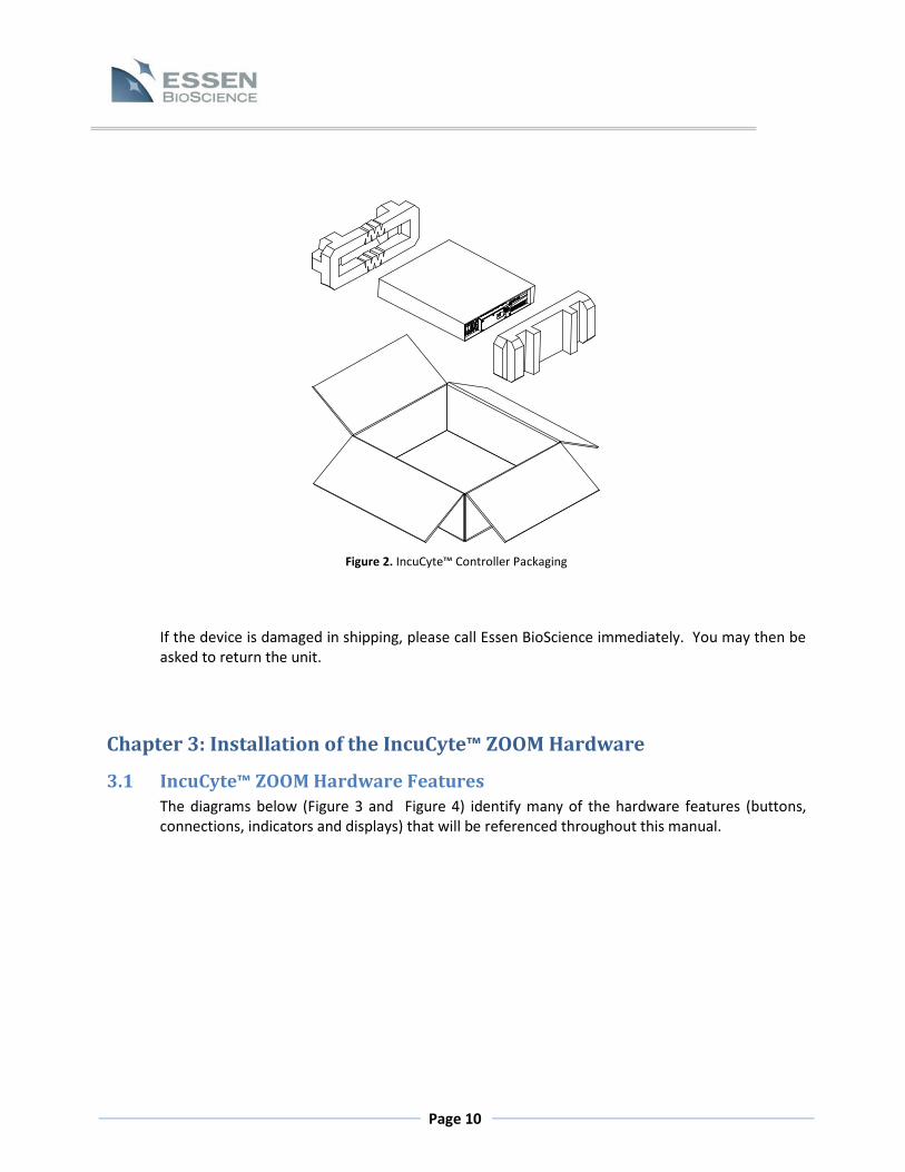
The controller should be removed from its box and bag in a similar fashion (see Figure 2). The controller box will contain the controller and, under most circumstances, it will also include a power cord appropriate for your local utilities. However, while Essen provides power cords compatible with most utilities, there will be instances in which Essen does not stock the compatible cord. In these rare circumstances, the purchaser will have to provide their own cord.
Figure 1. IncuCyte™ ZOOM Microscope Packaging
Page 10
If the device is damaged in shipping, please call Essen BioScience immediately. You may then be asked to return the unit.
Chapter 3: Installation of the IncuCyte™ ZOOM Hardware
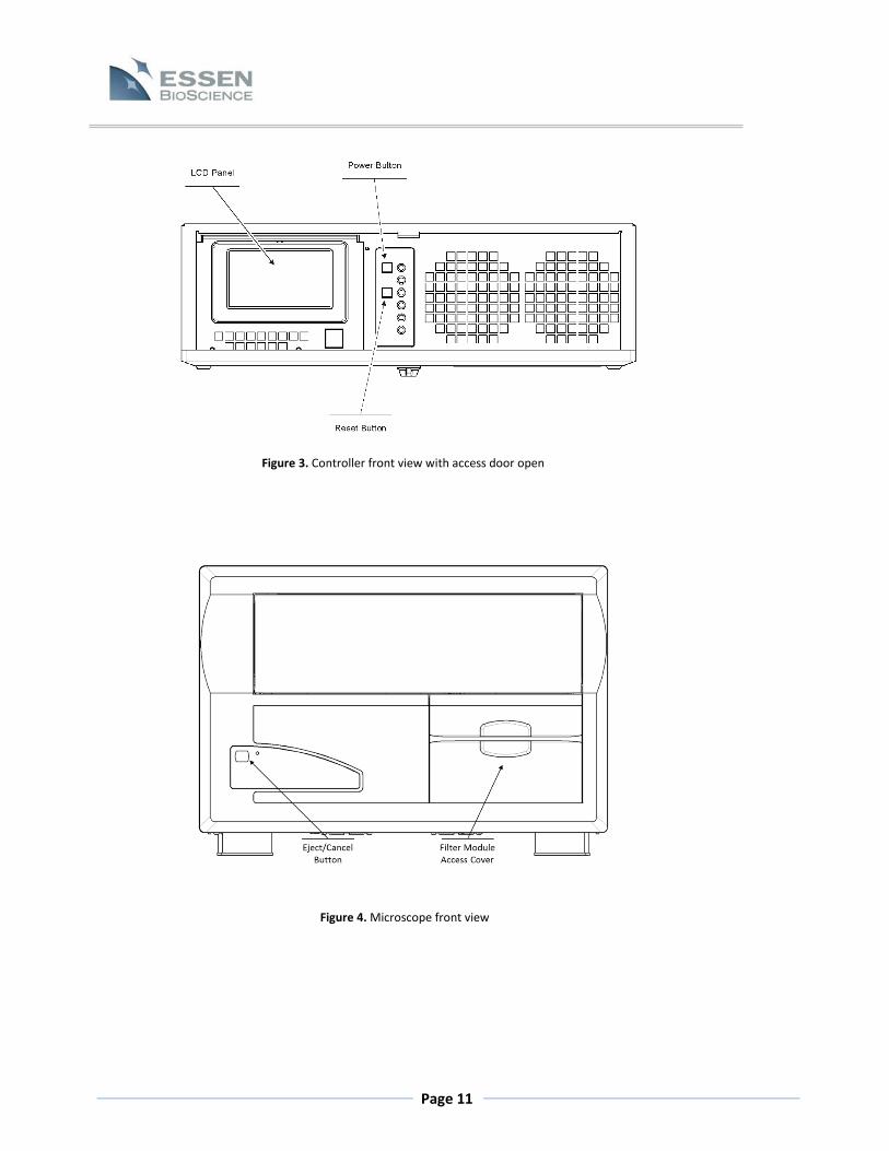
3.1 IncuCyte™ ZOOM Hardware Features The diagrams below (Figure 3 and Figure 4) identify many of the hardware features (buttons, connections, indicators and displays) that will be referenced throughout this manual.
Figure 2. IncuCyte™ Controller Packaging
Page 11
Figure 3. Controller front view with access door open
Figure 4. Microscope front view

Page 12
3.2 Removing the Shipping Pin The IncuCyte™ ZOOM ships with objectives and filter modules packed in a separate box. There is also a shipping pin installed to lock the microscope in place. It must be removed before the system installation can proceed. Remove the filter module access cover by pushing it down and pulling the cover out. The pin will be visible as in Figure 5 below. To remove the pin, depress the button in the center of the T handle and pull the pin straight up until it is free. Store the pin with the other ZOOM accessories so that it can be reused if the system needs to be shipped to another location or returned for service.
Figure 5. Microscope with access cover removed

Page 13
Figure 6. Microscope with shipping pin removed
3.3 Installing the Filter Module There are currently two types of filter modules available for your IncuCyte™ ZOOM, one is for
systems that collect phase images only (no fluorescence) and the other allows collection of dual
wavelength fluorescence. One of these modules will have been shipped in the accessories box
with your ZOOM.
With the filter module access cover removed, pull out the drawer about halfway in order to get
better access. Remove the plastic cover from the filter module mount screw hole and place the
module into the microscope. Press the module into place such that the connector on the module
engages the connector in the microscope. The module can then be secured in place using the
2.5mm T handle hex (Allen) wrench supplied. Replace the plastic cover in the module mount
screw hole. See the diagram below ( Figure 7).
Page 14
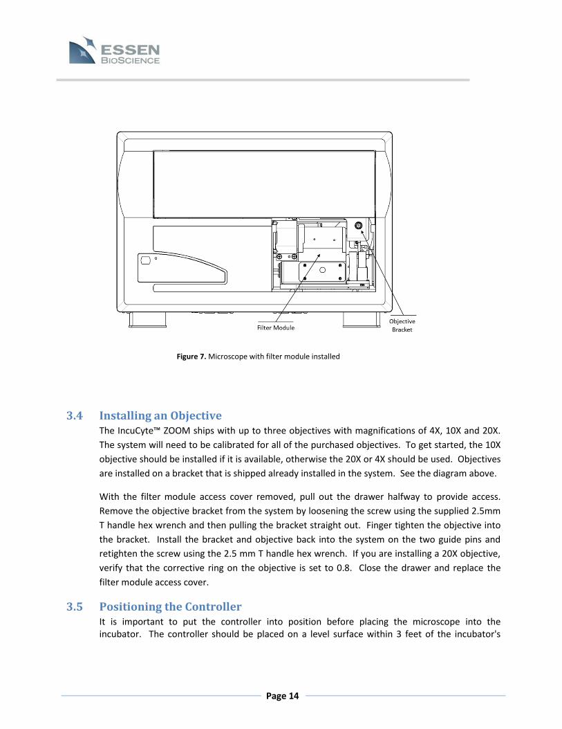
Figure 7. Microscope with filter module installed
3.4 Installing an Objective The IncuCyte™ ZOOM ships with up to three objectives with magnifications of 4X, 10X and 20X.
The system will need to be calibrated for all of the purchased objectives. To get started, the 10X
objective should be installed if it is available, otherwise the 20X or 4X should be used. Objectives
are installed on a bracket that is shipped already installed in the system. See the diagram above.
With the filter module access cover removed, pull out the drawer halfway to provide access.
Remove the objective bracket from the system by loosening the screw using the supplied 2.5mm
T handle hex wrench and then pulling the bracket straight out. Finger tighten the objective into
the bracket. Install the bracket and objective back into the system on the two guide pins and
retighten the screw using the 2.5 mm T handle hex wrench. If you are installing a 20X objective,
verify that the corrective ring on the objective is set to 0.8. Close the drawer and replace the
filter module access cover.
3.5 Positioning the Controller It is important to put the controller into position before placing the microscope into the incubator. The controller should be placed on a level surface within 3 feet of the incubator's

Page 15
WARNING! The top cover of the microscope should NEVER be used as a shelf and should NEVER be used to support a shelf.
IMPORTANT: After the microscope is placed in the incubator. Proceed IMMEDIATELY to the next two sections. To avoid large amounts of condensation on the unit it is desirable to connect and power the unit within a few minutes of installation.
cable port. The top of the incubator often works well. Do not, however, connect any of the controller cabling at this point.
3.6 Placing the Microscope into the Incubator When choosing a shelf for the microscope, keep in mind that flasks and plates are placed into the IncuCyte™ ZOOM cell drawer from above. For incubators that are at table height, a shelf installed near the bottom of the incubator is usually most convenient. Approximately 12.5 inches of height will be used by the instrument. In most incubators, this usually allows room for at least two shelves to be installed above the microscope. Remove all shelves above the targeted shelf before setting the microscope into the incubator. Feed the two cables from the microscope out through the cable access port on the back or side of the incubator. The cables can usually be routed up a corner of the incubator so as not to interfere with the installation of shelves above the microscope. A split stopper supplied with the unit can be used to plug the access hole around the cables. Shelves can be reinstalled above the unit as close to the incubators as the mounting brackets allow.
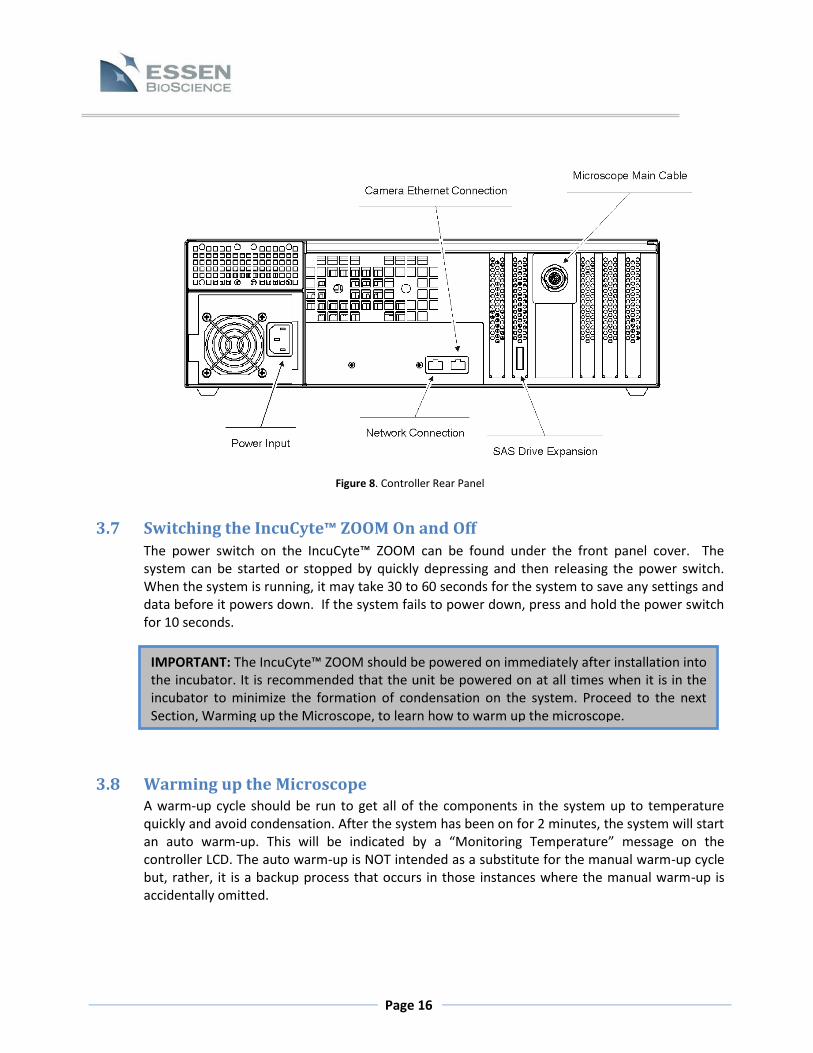
For connecting the cabling, see the rear panel of the IncuCyte™ ZOOM controller (Figure 8). There are two cables that connect the IncuCyte™ ZOOM controller to the microscope. These cables, which are fixed to the microscope, should be connected to the controller before the unit is powered on. The larger, circular style plug on the microscope main cable should be connected to the mating socket on the back of the controller. The second cable is a gigabit Ethernet interface to the digital camera in the microscope and it should be plugged into the mating connector labeled camera on the rear of the controller. The power cord for the unit can now be installed. Use only the AC power cord supplied or an equivalent cord with an IEC-320-C13 standard connector approved for operation at 5 amps and the appropriate voltage for your local power.
Page 16
IMPORTANT: The IncuCyte™ ZOOM should be powered on immediately after installation into the incubator. It is recommended that the unit be powered on at all times when it is in the incubator to minimize the formation of condensation on the system. Proceed to the next Section, Warming up the Microscope, to learn how to warm up the microscope.
3.7 Switching the IncuCyte™ ZOOM On and Off The power switch on the IncuCyte™ ZOOM can be found under the front panel cover. The system can be started or stopped by quickly depressing and then releasing the power switch. When the system is running, it may take 30 to 60 seconds for the system to save any settings and data before it powers down. If the system fails to power down, press and hold the power switch for 10 seconds.
3.8 Warming up the Microscope A warm-up cycle should be run to get all of the components in the system up to temperature quickly and avoid condensation. After the system has been on for 2 minutes, the system will start an auto warm-up. This will be indicated by a “Monitoring Temperature” message on the controller LCD. The auto warm-up is NOT intended as a substitute for the manual warm-up cycle but, rather, it is a backup process that occurs in those instances where the manual warm-up is accidentally omitted.
Figure 8. Controller Rear Panel

Page 17
CANCEL the auto warm-up by pressing the “Stop/Eject” button on the front of the microscope and start a manual warm-up. Use the LCD panel located on the front of the controller to start the manual warm-up and follow the steps indicated below:
1. Click on the “Menu” button on the LCD screen and select the “Tools” option from the list on the left.
2. Click on the “Warm-up” button from the newly displayed list of options.
3. Click on the “Go” button and select “Yes” to confirm that you want to start the warm-up.
The warm-up cycle will begin after a few seconds and will continue for approximately 45 minutes. The green activity light on the front of the microscope next to the “Eject/Cancel” button will be lit during the warm-up. A “Warming up” message will be displayed on the LCD in the top right corner along with information of time remaining until the warm-up is complete.
3.8.1 Auto Warm-up
In the event that the manual warm-up process is omitted (for instance, if the IncuCyte™ ZOOM is temporarily removed from the incubator, and the person replacing it forgets to run the manual warm-up procedure afterwards), then an auto warm-up process will be initiated. The auto warm-up is NOT intended as a substitute for the manual warm-up cycle but, rather, it is a backup process that occurs in those instances where the manual warm-up is accidentally omitted.
When auto warm-up starts, the microscope is powered on and the front-panel LED lights up until the camera achieves the requisite temperature. If the microscope is placed into the incubator cold, then the auto warm-up process is automatically triggered. Auto warm-up keeps the camera powered on for up to 45 minutes until it reaches a temperature slightly above that of the standard incubator temperature. Auto warm-up cannot occur if the controller is not powered on.
The auto warm-up cycle will be interrupted by scan. However, auto warm-up will resume if the camera has not achieved its target temperature after the interrupting scan has been concluded.
3.8.2 IncuCyte™ Controller Air Filter
The filter for the IncuCyte™ ZOOM controller is located behind the front panel (see Figure 9). Although this filter is easily accessible, it is NOT a consumable part, and Users should not attempt to exchange it themselves. If there are any questions about this filter, please contact Essen BioScience for more information.

Page 18
Chapter 4: Establishing Network Connections The IncuCyte™ controller houses an embedded control computer that must be connected to your network in the same way that ordinary PC’s running Microsoft Windows are connected. We recommend that you consult with your IT department during the network connection, configuration and verification processes. A standard Ethernet cable is used to connect the controller to a network hub or switch. The unit is equipped with two network ports. The leftmost port is used as the primary network interface to connect the IncuCyte™ controller to the network. The jack on the right is a port for the microscope camera Ethernet cable. See Figure 8 for details.
The controller is configured at the factory for automatic assignment of its IP address on a network using DHCP (Dynamic Host Configuration Protocol). Follow the procedures described in Section 4.1, DHCP Based Networks to connect to this type of network. If the network is not configured to assign IP addresses dynamically, then a static IP address must be assigned to the controller. See Section 4.2 (page 20), Static IP Based Networks, to reconfigure the IncuCyte™ controller for a fixed IP network.
4.1 DHCP Based Networks Turn off power to the unit, and connect the controller’s primary Ethernet port to the network with a standard Ethernet cable. Power on the controller and wait a few minutes before verifying the controller is networked correctly.
If connected correctly, the controller will appear as a computer on the Microsoft Windows Network as a member of the “Workgroup” group of computers. Assume that the controller is assigned the name ZOOMXXXXX in the factory, where XXXXX is the 5-digit serial number of the controller. This serial number is found on a label on side of the controller.
Figure 9. IncuCyte™ Front Panel

Page 19
To verify that the ZOOMXXXXX controller has been successfully added to the network, a Windows-based PC (hereby referred to as the “PC”) on the same network is required. These verification methods are discussed separately for Windows Vista/7 and Windows XP PC’s.
4.1.1 Verifying the IncuCyte™ Controller Network Connection: Windows Vista or
Windows 7
1. Under the Windows “Start” menu, select “Network” (Vista) or “Computer” (Windows 7).
a. Windows 7 only: On the left side of the window there is a list of destinations (“Favorites”, “Libraries”, etc.). Look for the “Network” destination and select this by left-clicking.
2. Look for the computer named ZOOMXXXXX (recall that XXXXX is the 5-digit controller serial number). If you find it in the window, then the controller was successfully added to the network, and you are done. If not, you should attempt to find the controller on the network by continuing to the next step.
3. At the top of the window there is a text area that reads “► Network ►”. Left-click in an empty area to the right of this text and type the following: \\ZOOMXXXXX followed by the “Enter” key.
4. If the controller is found on the network, you will be prompted for a User name and password. Press the “Cancel” button to exit. If the controller is not found, then a “Cannot Find” message will be displayed after a brief search period.
4.1.2 Verifying the IncuCyte™ Controller Network Connection: Windows XP
1. Open “My Computer” from the PC’s Windows Start menu.
2. Under the heading “Other Places” on the left side of the window, open “My Network Places.”
3. Under the heading “Network Tasks” on the left side of the window, click once on
“View workgroup computers.”
4. Look for the computer named ZOOMXXXXX (recall that XXXXX is the 5-digit controller serial number). If you find it in the window, then the controller was successfully added to the network, and you are done. If not, you should attempt to find the controller on the network by continuing to the next step.
5. Verify that the “Address” toolbar is displayed at the top of the window. Under the
“View” menu time at the top of the window, verify that the “Toolbars - > Address Bar” menu item has a check mark next to it.
6. Type the following in the “Address” box at the top of the window: \\ZOOMXXXXX.
Page 20
NOTE: This version of the IncuCyte™ Control Software is not backwards compatible with IncuCyte™ microscopes that are running earlier versions of the software. Contact Essen BioScience technical support for instructions for updating controller software.
7. Click on the “Go” button to the right of the address bar. If the controller is found on the network, you will be prompted for a User name and password. Press the “Cancel” button to exit. If the controller is not found, then a “Cannot Find” message will be displayed after a brief search period.
4.2 Static IP Based Networks In order to reconfigure the IncuCyte™ ZOOM controller for a static IP address, a direct connection must first be made to the controller. In order to accomplish this you will need to connect a monitor, keyboard and mouse to the controller. To gain access to the monitor, keyboard and mouse ports you need to unscrew the two screws on the back of the controller and remove the back cover (See Figure 8).
With the controller powered down, connect the monitor, keyboard and mouse to the controller. After connecting, power up the controller. Once Windows has booted up you can log in with a User name "ZoomAdmin" and the Essen-provided password.
Recall that the ultimate goal is to configure the controller’s primary Ethernet port with a static IP address selected for your corporate network. Once on the desktop, the controller’s primary Ethernet port can be configured with a static IP address in the same way that the PC’s primary port was configured. Use the Windows 7 instructions for the controller configuration. After configuring the primary Ethernet port, log off of the controller’s desktop. Unplug the monitor, keyboard and mouse from the back of the controller and reinstall the cover on the back of the controller.
Chapter 5: Installation of the IncuCyte™ Control Software The IncuCyte™ ZOOM control software is used to both configure the instrument to collect data and for post-collection viewing and analysis of these data. This software is designed to run on PC’s running Windows XP, Windows Vista or Windows 7 and requires an Administrator account to install.
Contact Essen BioScience Support (refer to section 2.3 for support contact information) to get the most recent version of the software. Once downloaded, run the installer by double clicking on the installer file.
5.1 IncuCyte™ Control Software Installation using Windows XP 1. Review the license agreement. To continue installation you must agree. 2. Select components you want to install. 3. Choose a destination folder and Install. 4. Install the Windows Media Player Codecs. (Required to save movies).

Page 21
NOTE: It is possible you will get a message titled “Windows Media player 10” stating that “This version of Windows Media Technologies is incompatible with this version of windows….” This message can be disregarded. Just click “Cancel”. The incompatibility message communicates that the machine already has a newer version of Windows Media Codecs (for movie generation). It will be followed by a message entitled “Windows Media Player Codecs Setup” stating that “The Codec package for the 7+ Player has been installed successfully.”
5. If prompted, install the Windows Media Encoder. (Required to save movies). 6. Close the installer when completed.
5.2 IncuCyte™ Control Software Installation using Windows Vista and
Windows 7 1. Review the license agreement. To continue installation you must agree. 2. Select components you want to install. 3. Choose a destination folder and Install. 4. If prompted, install the Windows Media Encoder. (Required to save movies). 5. Close the installer when completed.
5.3 Connecting
5.3.1 Setting the Date and Time
The IncuCyte™ ZOOM controller settings will be synchronized with the local computer at the time of installation. It is unlikely that any further synchronization will be required after that point. However if, for some reason, synchronization is required at a later date, the IncuCyte™ software will issue a prompt to this effect. The prompt will appear after login but before the software is launched. The exact verbiage of the prompt will depend on which settings are in a state of disagreement. Figure 10 displays the window that will appear if an individual at the User or Guest permission level logs onto the software and Time Zone synchronization is required. A slightly different message will appear if the individual is at the Administrator permission level.
Figure 10. Time Zone Synchronization Window at the User or Guest Permission Level
Page 22
NOTES: We strongly recommend that ONLY individuals at the Administrator permission level implement changes to the controller time settings.
Tine or Time Zone synchronization is ONLY required if the IncuCyte™ software issues a prompt, such as the example displayed in Figure 10.
5.3.2 Establishing User Accounts
Essen BioScience will establish the initial Administrator account. Additional Users can be created using the Create User function. All IncuCyte™ Users must have an account on each instrument they wish to use. However, we recommend that the number of Users with Administrator level permission be kept to a minimum.
To establish new User accounts, click on the Administer IncuCyte™ task bar in the upper left corner of the main window. The available Administrator functions are organized within a series of tabs. Select the Accounts tab to access password and accounts information.
The Change Password menu allows Users to set and change their own passwords. This function is available to Users at all permission levels. The Create User and Delete User functions, however, are only available to Users with the Administrator permission level. New Users must have a unique User name. Passwords are case sensitive, and new Users should be encouraged to change their password the first time they log on. When creating a new User, it is important to select an appropriate Permission Level. Users with an Administrator Permission Level have all of the functions of the IncuCyte™ control program available to them. A User with a User Permission Level is able to change his/her password, view device information, configure the device to collect data and perform all post-collection analysis (view, plot, annotate, etc). A User with “Limited User” Permission level can perform all tasks that the “User” can do except configuring the device to collect data. The “Guest” Permission level is one step below the “User” level in that guests cannot configure the device to collect data. The software functions available at the various permission levels are summarized in Table 1.

Page 23
Table 1. User Account Access
Function Guest Limited User User Admin
Scheduling Access No No Yes Yes
Admin Access No Limited Limited All
Edit Vessel Documentation No Yes Yes Yes
Archive Vessels No Yes Yes Yes
Delete Archives from ZOOM-Attached Storage
No Their own Their own Any
Delete Archives from browsed to from “My Computer”
Yes (with warning)
Yes (with warning)
Yes (with warning)
Yes (with warning)
Delete Vessels No No Their own Any
Launch Analysis Jobs No Yes Yes Yes
Delete Analysis Jobs No Their own Their own Any
Add Processing Definitions No Yes Yes Yes
Edit Processing Definitions No Their own Their own Any
Delete Processing Definitions No Their own Their own Any
Add to Image Collections No Their own Their own Any
Edit Image Collections No Their own Their own Any
Delete Image Collections No Their own Their own Any
View Diagnostic Scan Metrics No No No Yes
5.4 Remote Administration of the Controller The IncuCyte ™ ZOOM controller consists of a single-board computer running a Windows-based embedded operating system. This computer is dedicated to controlling the IncuCyte™ ZOOM hardware and providing remote access to the data collected by the instrument. To insure reliable and proper operation of your IncuCyte™, the factory settings of the controller operating system should not be altered. However, we recognize that there may be instances when it is desired or even required to log onto the embedded controller desktop. Some examples include:
Renaming the controller from the factory-set name Configuring the primary Ethernet port with a static IP address Installing anti-virus and/or firewall software Installing Essen-recommended Windows updates
The IncuCyte™ controller ships with a unique Administrator password for accessing the controller’s Windows desktop. Essen BioScience maintains a record of this password, so we strongly discourage you from renaming the Administrator password. We also recommend that this password be protected and that the controller operating system be accessed only out of necessity. Altering the controller operating system as little as possible is the best way to guarantee stability of the software that controls the IncuCyte™ ZOOM.
The easiest method for accessing the controller desktop is through the Windows “Remote Desktop Connection” tool. Windows XP Users can access this utility through the Windows Start menu under the “Programs -> Accessories -> Communications” menu. Users of Windows Vista and Windows 7 will find the utility in the “All > Programs > Accessories” menu.

Page 24
IMPORTANT: Always use the “Disconnect” option and not the “Log Off” option when terminating the Remote Desktop Connection via the controller Start menu.
Run the “Remote Desktop Connection” software and type in the name of the IncuCyte™ ZOOM controller in the “Computer” edit box. If connecting for the very first time, the name used will be the factory-set name. Make sure that you have connected and verified that the controller is on the network (see Sections: 4.1.1 and 4.1.2). Press the “Connect” button and wait for a Windows login prompt. It may take as long as 15 seconds before the prompt appears. Log into the controller with a User name "ZoomAdmin" and the Essen-provided password. The controller operating system should contain the necessary components required to rename the computer, configure the primary Ethernet port, install security software, etc. Please consult with your IT department for answers to questions related to your local network configuration and security software.
Chapter 6: Calibrating the IncuCyte™ ZOOM System
6.1 System Calibration Before using the IncuCyte™ ZOOM for the first time, a calibration procedure must be performed. This procedure ensures that the motion of the IncuCyte™ ZOOM microscope is accurate and repeatable such that images are obtained within their proper, target locations. This is especially important when acquiring images in 96 and 384-well plates. The calibration procedure requires up to 1.5 hours, and it utilizes a special calibration tray that is shipped out with the unit (Figure 11). The calibration tray is the same size and is inserted in the same fashion as the regular trays. Each of the three tray positions (front, middle and rear) must be calibrated individually. What follows is an overview of the calibration procedure.
Figure 11. The Calibration Tray
Page 25
NOTE: Calibration can ONLY be performed by a User at the Administrator Permission level.
Place the Calibration Tray into one of the tray positions (the order in which tray positions are calibrated is not important, but all 3 must be calibrated).
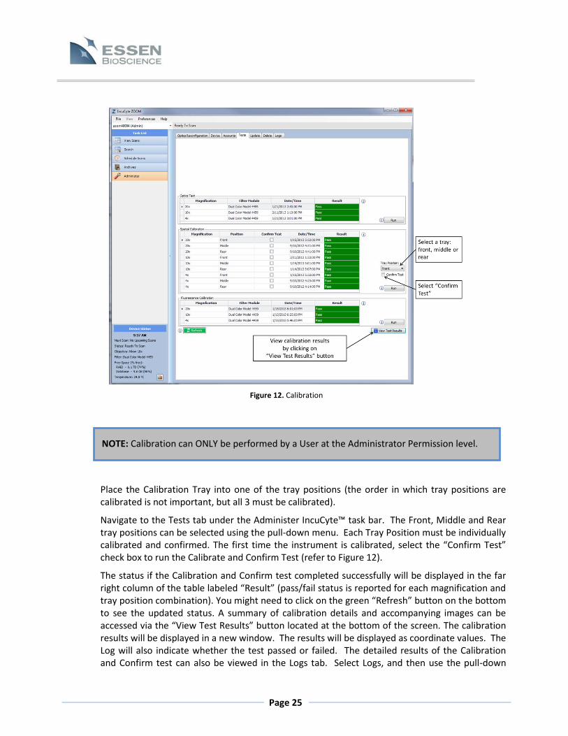
Navigate to the Tests tab under the Administer IncuCyte™ task bar. The Front, Middle and Rear tray positions can be selected using the pull-down menu. Each Tray Position must be individually calibrated and confirmed. The first time the instrument is calibrated, select the “Confirm Test” check box to run the Calibrate and Confirm Test (refer to Figure 12).
The status if the Calibration and Confirm test completed successfully will be displayed in the far right column of the table labeled “Result” (pass/fail status is reported for each magnification and tray position combination). You might need to click on the green “Refresh” button on the bottom to see the updated status. A summary of calibration details and accompanying images can be accessed via the “View Test Results” button located at the bottom of the screen. The calibration results will be displayed in a new window. The results will be displayed as coordinate values. The Log will also indicate whether the test passed or failed. The detailed results of the Calibration and Confirm test can also be viewed in the Logs tab. Select Logs, and then use the pull-down
Figure 12. Calibration

Page 26
menu under Log Type to select Tests. The calibration results will be displayed in the large window below. If no results are visible, press the Refresh button at the bottom of the screen to update the log. Check to be sure the test passed for all three tray positions before proceeding to Chapter 7. If the calibration was not successful, cell culture monitoring will not produce quality results.
6.2 Fluorescence Calibration A fluorescence calibration kit will be provided when a dual fluorescence filter module is purchased with the IncuCyte™ ZOOM, and the instrument will be calibrated at the time of installation. It is currently recommended that the instrument be recalibrated twice a year. The fluorescence calibration kit includes reagent sufficient for multiple calibrations as well as three calibration slides. These calibration slides are disposable and should be used only once. New calibration kits can be purchased from Essen BioScience. Follow these steps to perform the fluorescence calibration: 1. Place a calibration tray in the front position of the IncuCyte™ ZOOM. Fluorescence
calibration requires use of the front tray position, and the remaining positions can be occupied with trays at the time of calibration.
2. Load a calibration slide with supplied dye. Use 40 µl dye per slide. Place the pipet tip at one
end of the slide window and expel the liquid dye. The liquid will wick into the slide window. After all the dye has been expelled, use the pipet to transfer a small amount of dye to the other end of the window to be sure it is completely filled. Avoid getting any dry spots in the window as this will interfere with proper calibration. Place the calibration slide in slide cutout of the calibration tray. The orientation of the slide within the cutout position is not important.
3. Select the Tests tab under the Administer IncuCyte™ tasks bar. Then, select the Fluorescence
Calibration test. Press the Run button. A new window will open to confirm that the IncuCyte™ is properly configured to run the test. Press the Yes button to start the calibration. See Figure 13.
The calibration procedure will begin. Fluorescence Calibration requires ~ 8 minutes. Calibration status will be indicated at the top of the IncuCyte™ software window and in the status box at the bottom left.

Page 27
Figure 13. Fluorescence Calibration
6.2.1 FLR Calibration Results
When the calibration is complete the status of the Fluorescence Calibration completed successfully will be displayed in the far right column of the table labeled “Result” (pass/fail status is reported for each magnification). You might need to click on the green “Refresh” button on the bottom to see the updated status. A summary of calibration details and accompanying images can be accessed via the “View Test Results” button located at the bottom of the screen. The calibration results will be displayed in a new window. The detailed results can also be viewed under the Logs tab, Log Type: Test. The log will also state whether or not the calibration passed. If the calibration failed, the log will include recommendations to avoid potential issues the next time through.
Chapter 7: Cell Culture Monitoring and Data Analysis
7.1 Introduction The IncuCyte™ ZOOM introduces an innovative platform to acquire, analyze and quantify images from living cells that remain unperturbed by the detection method for repeated measures over long periods of time; features we refer to as Live Content Imaging. In addition, IncuCyte™ ZOOM has a powerful database designed to make it simple for Users to search and retrieve experimental data using a unified search tool.
The design of the IncuCyte™ ZOOM software provides flexibility in designing cellular assays as well as providing easy to understand, sophisticated analysis tools. These analytical tools allow

Page 28
Users to translate qualitative observations to quantitative data in order to facilitate data driven decision making. Simple image export options, channel blending and unmixing, and movie making tools provide a means to easily integrate IncuCyte™ ZOOM generated data into presentations, posters, and publications. The basic workflow of setting up an experiment from scheduling to experimental results for both assay development and performing established assays is represented below.
All aspects of live content imaging using the IncuCyte™ ZOOM software are described in detail within this chapter.
7.2 User Interface Once connected to an IncuCyte™ ZOOM, the User can easily maneuver throughout the distinct parts of the software. The Task List located on the left side of the screen, enables access to administrative tasks (device control, logs, User accounts, and vessel deletion), vessel scheduling , search options, and vessel archiving . The software also displays the status of the connected IncuCyte™ ZOOM device including objective configuration, device temperature, drive space indicator, and scan status.

Page 29
The IncuCyte™ ZOOM Software was designed to allow Users to efficiently navigate throughout the program by clicking on text as well as graphical icons and images. Users should take the time to investigate the functionality of the IncuCyte™ software interface as well as moussing over the information icons found throughout the window screens.
7.3 Scheduling Scans and Loading Vessels To initiate any assay, begin by selecting the Schedule Scans option located on the left side task list. Once selected, the scheduling interface will enable the User to either schedule scans on a 24-Hour Repeating schedule or a single Scan on Demand.
7.3.1 24-Hour Repeating The 24-Hour Repeating Schedule allows Users to define a set interval for acquisition times. Once the 24-Hour Repeating vertical tab is selected, you will be required to enter information that defines your specific assay.
7.3.1.1 Vessel selection: In the Drawer Setup pane, determine which tray position (front, middle or rear) you would like to place your vessel and then use the “Add Vessel” button to select a vessel type.
1. Once the vessel selection window is open, you will be able to search a table for your vessel of choice. The IncuCyte™ software automatically recognizes the tray type required for each vessel and will display the tray type below the vessel selection table.
2. At this time, highlight an empty vessel position within the tray and click the “OK” button. Once the vessel selection is completed the Scan Setup and vessel Properties tabs become activated.
7.3.1.2 Scan Setup Tab: At this time select the channels required for image acquisition of your vessel, as well as the scan mode, scan pattern, spectral un-mixing, and analysis job setup. Refer to Table 2 for details.
Page 30
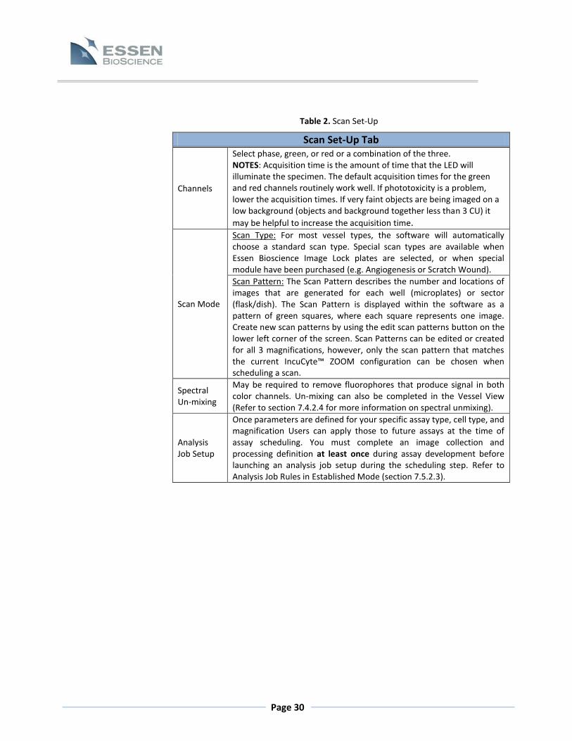
Table 2. Scan Set-Up
Scan Set-Up Tab
Channels
Select phase, green, or red or a combination of the three. NOTES: Acquisition time is the amount of time that the LED will illuminate the specimen. The default acquisition times for the green and red channels routinely work well. If phototoxicity is a problem, lower the acquisition times. If very faint objects are being imaged on a low background (objects and background together less than 3 CU) it
may be helpful to increase the acquisition time.
Scan Mode
Scan Type: For most vessel types, the software will automatically choose a standard scan type. Special scan types are available when Essen Bioscience Image Lock plates are selected, or when special module have been purchased (e.g. Angiogenesis or Scratch Wound).
Scan Pattern: The Scan Pattern describes the number and locations of images that are generated for each well (microplates) or sector (flask/dish). The Scan Pattern is displayed within the software as a pattern of green squares, where each square represents one image. Create new scan patterns by using the edit scan patterns button on the lower left corner of the screen. Scan Patterns can be edited or created for all 3 magnifications, however, only the scan pattern that matches the current IncuCyte™ ZOOM configuration can be chosen when scheduling a scan.
Spectral Un-mixing
May be required to remove fluorophores that produce signal in both color channels. Un-mixing can also be completed in the Vessel View (Refer to section 7.4.2.4 for more information on spectral unmixing).
Analysis Job Setup
Once parameters are defined for your specific assay type, cell type, and magnification Users can apply those to future assays at the time of assay scheduling. You must complete an image collection and processing definition at least once during assay development before launching an analysis job setup during the scheduling step. Refer to Analysis Job Rules in Established Mode (section 7.5.2.3).
Page 31
7.3.1.3 Vessel Properties Tab: Vessel properties are used to describe the assay being scheduled (refer to Table 3). These properties will be used when searching for and viewing scanned vessels.
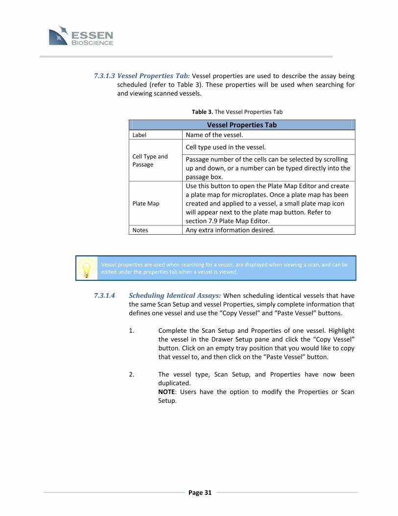
Table 3. The Vessel Properties Tab
Vessel Properties Tab Label Name of the vessel.
Cell Type and Passage
Cell type used in the vessel.
Passage number of the cells can be selected by scrolling up and down, or a number can be typed directly into the passage box.
Plate Map
Use this button to open the Plate Map Editor and create a plate map for microplates. Once a plate map has been created and applied to a vessel, a small plate map icon will appear next to the plate map button. Refer to section 7.9 Plate Map Editor.
Notes Any extra information desired.
7.3.1.4 Scheduling Identical Assays: When scheduling identical vessels that have the same Scan Setup and vessel Properties, simply complete information that defines one vessel and use the “Copy Vessel” and “Paste Vessel” buttons.
1. Complete the Scan Setup and Properties of one vessel. Highlight
the vessel in the Drawer Setup pane and click the “Copy Vessel” button. Click on an empty tray position that you would like to copy that vessel to, and then click on the “Paste Vessel” button.
2. The vessel type, Scan Setup, and Properties have now been duplicated. NOTE: Users have the option to modify the Properties or Scan Setup.
Page 32
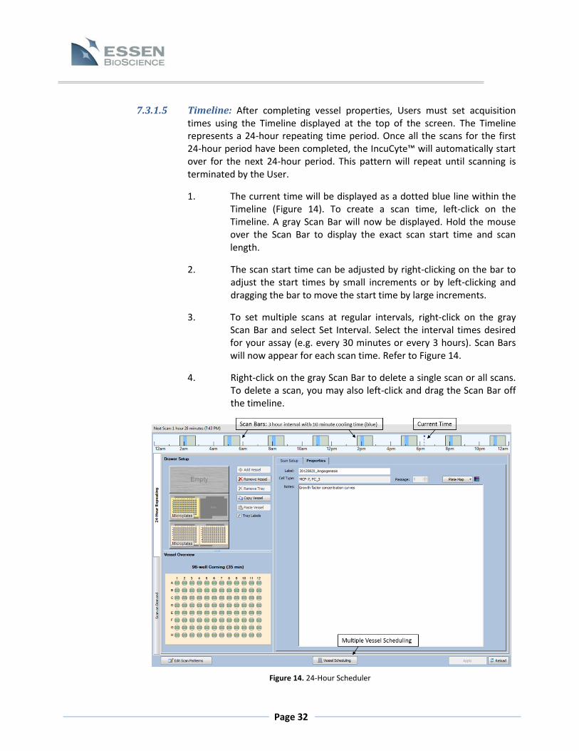
7.3.1.5 Timeline: After completing vessel properties, Users must set acquisition times using the Timeline displayed at the top of the screen. The Timeline represents a 24-hour repeating time period. Once all the scans for the first 24-hour period have been completed, the IncuCyte™ will automatically start over for the next 24-hour period. This pattern will repeat until scanning is terminated by the User.
1. The current time will be displayed as a dotted blue line within the Timeline (Figure 14). To create a scan time, left-click on the Timeline. A gray Scan Bar will now be displayed. Hold the mouse over the Scan Bar to display the exact scan start time and scan length.
2. The scan start time can be adjusted by right-clicking on the bar to adjust the start times by small increments or by left-clicking and dragging the bar to move the start time by large increments.
3. To set multiple scans at regular intervals, right-click on the gray Scan Bar and select Set Interval. Select the interval times desired for your assay (e.g. every 30 minutes or every 3 hours). Scan Bars will now appear for each scan time. Refer to Figure 14.
4. Right-click on the gray Scan Bar to delete a single scan or all scans. To delete a scan, you may also left-click and drag the Scan Bar off the timeline.
Figure 14. 24-Hour Scheduler

Page 33
7.3.1.6 Multiple Vessel Scheduling: When scanning multiple vessels, the “Vessel Scheduling” button at the bottom of the Schedule Scans screen allows the User to insert cooling (idle) times between vessel scans and customize the order in which IncuCyte™ scans vessels. Using the Auto-Cool function is recommended and allows for the most efficient vessel scheduling. NOTE: The Multiple Vessel Scheduler is ONLY needed if Users plan to introduce cooling times or need to change the order of scanned vessels.
7.3.1.7 Apply Schedule: When the Scan Setup, vessel Properties and Scan Time(s) have been set, select the “Apply” button at the bottom of the screen. A window will appear confirming that scanning parameters have been applied. NOTE: Pressing the “Reload” button at the bottom of the Schedule Scans screen will reset all settings (physical layout, properties, scan times, etc.) back to the way they were prior to the last time the “Apply” button had been selected.
7.3.1.8 Place Tray and Vessel in IncuCyte™: Place the appropriate tray (refer to section 7.8.1 Selecting and Placing Trays) and vessel in the pre-determined position within the IncuCyte™. Allow time for the vessel to equilibrate to the temperature of the incubator prior to initiating scans (approximately 15- 20 minutes).
7.3.1.9 Terminating Scan Times and Deleting Vessels:
1. To terminate scanning, right-click on the Scan Bar to be deleted and either select delete (for that specific scan time) or delete all (to remove all scan times). Select the “Apply” button at the bottom of the screen. A scan can also be manually terminated by pushing the Stop button on the front of the IncuCyte™. Pushing the Stop button will abort the scan that is ongoing at that time. However, if scanning is terminated in this way, the IncuCyte™ will start scanning again at the next scheduled scan time. The ONLY way to terminate all future scans is by deleting all the Scan Bars and then selecting “Apply”.
2. To remove a vessel from the schedule, simply highlight the desired vessel and click on the “Remove Vessel” button. Select the “Apply” button on the bottom of the screen.

Page 34
7.3.2 Scan on Demand In addition to the 24-Hour Repeating scan schedule, Users also have the ability to scan in the Scan on Demand mode. Simplistically, this means that the IncuCyte™ can be used to scan individual vessels at times when the IncuCyte™ is not scanning. This includes both periods in between regularly scheduled scans in the 24-Hour Repeating scheduler, as well as in designated Cooling Times. Scan on Demand allows Users to scan only one vessel in one tray position at a time.
7.3.2.1 Properties: Once the Scan on Demand vertical tab is selected, the following properties must be entered into the scheduler prior to scanning:
Tray Type Tray Position Cutout Position Vessel Type Scan Type Scan Pattern Channel Selection
7.3.2.2 Label and Unique ID: As with the 24-Hour Repeating schedule, vessel Properties (label, cell type) are used to both describe the vessel and searching for the vessel. In addition to a Label, Users can also supply a Unique ID to each vessel. This Unique ID can either be generated manually by typing or pasting information into the Unique ID field, or a Unique ID correlating to the current year/day/time will be assigned to the Scan on Demand vessel. This information can be used to link subsequent scans together. However, it is important to note that if the User fails to type in, or select (using the “Load” button) the correct Unique ID, scans will not be linked together, and cannot be accomplished post scanning.
7.3.2.3 Timeline: Within the Scan on Demand scheduler, the 24-Hour Repeating scan schedule (including all of the time bars) will be faded to the background, but will remain clearly visible.
1. The current time will be indicated as in the 24-Hour Repeating scheduler,
but will be followed by the yellow Scan on Demand Time Bar. NOTE: If the Scan on Demand Time Bar is red, this means that the Scan on Demand scan time overlaps with a scan time in the 24-Hour Repeating scheduler. Clicking on the red “Scan” button will result in an error.
2. Similar to the 24-Hour Repeating schedule, the width of the time bar will
correlate to the amount of time required to scan the vessel inserted into the Scan on Demand Tray. NOTE: The estimated time (indicated by the width of the yellow bar) to scan in the Scan on Demand mode is ≈20% longer than the estimated

Page 35
time in the 24-Hour Repeating scheduler. This additional time is required so that the User has time to replace the Scan on Demand vessel with the 24-Hour Repeating vessel.
7.3.2.4 Initiate Scan: Scanning using the Scan on Demand Scheduler is initiated by clicking the red “Scan” button.
7.4 Finding and Viewing Scanned Vessels After scans have been generated there are two ways to search and view your vessel of interest;
using View Scans option or the Search option . Once you have located your vessel using either the View Scans or Search tools, simply double-click on the vessel or use the “View Vessel” button on the lower right-corner of the window.
7.4.1 Finding Scanned Vessels
7.4.1.1 View Scans Tab: When the ZOOM IncuCyte™ software is launched, it opens by default to the View Scans screen. The first time the software is opened, the screen will be empty. However, once scans have been performed, the software will open to show the very last scan that was completed, as well as a Time Tree that lists the times and dates for all completed scans. NOTE: The View Scan screen is recommended for recently scanned vessels.
1. Click through the Time Tree to find completed scans generated on the device.
2. The center of the View Scan screen will display the Drawer Setup for that
particular scan time. Highlight the vessel of interest to display vessel properties to the right side of the screen.
3. Once your vessel of interest is located, either double-click on the vessel
or highlight the vessel and click on the “View Vessel” button in the lower right-hand corner of the screen.

Page 36
7.4.1.2 Search Tab: Scanned vessels can also be found by using the Search option found in the left task list pane. Once the Search screen is displayed, Users can search the entire Scanned Vessels table using the “Find” field or search within individual columns. The searching tools within the IncuCyte™ ZOOM software auto filters the table as soon as Users begin typing (at the beginning and within words), thus quickly narrowing down to a limited list of scanned vessels. Users can also place quotation marks around search terms in order to search the complete string. NOTE: Searches are NOT case sensitive. 1. Using the “Find” field, searches the entire Scanned Vessels table. Use the
Clear button located next to the Find field to remove filter results.
2. Search a specific column by clicking on the first row of the column. Column searching offers the auto sort when typing as well as multiple other functions which are listed in the table below. Refer to Table 4 for details. NOTE: Because the column search tools use the “and” function to filter, Users are able to filter scanned vessels using multiple columns. For example, you can use the User Column to narrow down to an individual, and then sort using other column fields such as Label, Color Data, or Cell Type.
Table 4. Column Search
Column Search Tools
Right-Click Allows you to sort and customize the column. For example you can sort, edit the script language, or remove or add a column.
Left-Click Left-click on the funnel icon in the upper right corner to filter.
or Ascending or descending sort tool.
3. Filtering using the Start Date/Time column requires you to right-click on
the funnel icon in the upper right corner. A calendar is displayed, showing the current month and day. To drill out, simply click on the month. This then displays a yearly calendar by month. You can further drill out by clicking on the year.
4. To clear a filtered column search in order to begin a new search, click on
the “x” in the lower left corner of the Search screen.
Page 37
5. Once your vessel of interest is located, either double-click on the listed vessel or use the “View Vessel” button in the lower right-hand corner of the screen.
7.4.2 Vessel View Once the vessel of interest is opened, the Vessel View window opens. The View Vessel window allows Users to view images collected, export images or movies, and update vessel associated properties.
7.4.2.1 Menu Bar: The Vessel View menu bar includes drop down menus for “Utilities” and “View”. The “Utilities” drop down menu allows Users to export images, movies, or an image set (refer to section 7.7 Exporting Images and Movies). The “View” drop down menu allows Users to display or remove vessel properties from the vessel image located at the top, center of the screen.
7.4.2.2 Time Tree: The Time Tree lists only the times and dates for all completed scans for that vessel. By selecting a time, the corresponding image will be displayed. View images from a specific scan time by clicking directly through the Time Tree or by using the forward or back buttons located below the Time Tree.
7.4.2.3 Vessel Image: The selected flask, dish or microplate is represented to the right of the Time Tree. Use the representative vessel display to view the images in different sectors/wells by selecting them with the mouse.
7.4.2.4 Image Tab: Displays the image from the scan time selected from the Time Tree and the sector/ well selected from the vessel display. Under the Image display tab Users are able to select, de-select, or adjust the image channels.
Adjust Image Controls
Use the brightness and contrast sliders to adjust image quality for the Phase channel.
The Fluorescence sliding “Weight” bars allow the User to adjust the display characteristics of fluorescence components within an image. Adjusting the display settings will affect which components of an image will be displayed as fluorescent, and also the brightness of those fluorescent images relative to each other. It will NOT affect the absolute (calibrated) fluorescence values.

Page 38
Calibrated fluorescence values are measured in terms of pixel brightness using Calibrated Units (CU’s). The fluorescence Min/Max Intensity settings can be adjusted either using the Auto-Scale function or via Manual Adjustment.
Auto Scale tries to assign optimum Min/Max settings for a particular image. Auto scaling is easy (just press the “Auto Scale” button), and in many cases the Auto Scale settings will be adequate. There are times when the auto scale derived Min/Max settings for one image will not represent the best settings for other images. If the “Always” box next to the “Auto-Scale” button is checked, then every time a new image is selected it will be automatically Auto-Scaled rather than using the values from the previous image. If a movie is generated, each image within the movie can be individually auto scaled (refer to section 7.7.2).
To manually adjust the fluorescent intensity values either type new
values directly into the Min/Max intensity boxes and press the “Enter” key, or use the arrows to scroll through values. Selecting a Minimum and Maximum Intensity “clips” the brightness at which fluorescent components will be displayed. Minimum Intensity: Any portion of the image with a pixel intensity value less than or equal to the Minimum Intensity will be assigned a relative brightness equal to the darkest possible value in the image (in this case black). Maximum Intensity: Any portion of the image with a pixel intensity greater than or equal to the Maximum Intensity will be assigned a relative brightness equal to the brightest possible value for the display (in this case, bright green). All portions of the image with pixel intensities between the Minimum and Maximum Intensity values will be assigned intermediate degrees of brightness.
Whether Min/Max settings are set manually or via the Autoscale
function, they will remain unchanged until manually re-adjusted or re-autoscaled on a different image. Therefore, the Min/Max settings applied to the original image will be applied to all subsequent images that are viewed within the same vessel at all scan times or even to images from different vessels. If images are combined to generate movies, each frame of the movie will contain an image with the same Min/Max settings.
Tools The Tool task pane located to the right of the image allows you to zoom in or out of an image by using the slider bar. Dragging the slider bar will zoom to the center of the image; however, the area of the zoomed image being displayed can be changed by grabbing the image and dragging it with the

Page 39
mouse. Alternatively, it is possible to zoom directly to a specific area within the image by scrolling the mouse wheel over the area of interest.
The Tool task pane also includes a measurement tool. Use Measurement
Mode to make linear measurements within the image. To turn Measurement Mode on or off, click on the ruler icon .
Spectral Unmixing Spectral unmixing may be required to remove fluorophores that produce signal in both color channels. These properties should be saved prior to adding images to an image collection or performing an analysis. NOTE: It is important to perform the spectral unmixing in small increments to determine the appropriate value. Figure 15 below illustrates spectral unmixing.
Top Row: Appropriate removal of the red fluorophore from the green channel using the spectral unmixing tool. Bottom Row: We lowered the green fluorescent channel to show the difference between optimized and overcorrected spectral unmixing. Using the NucLight-Red A549 cell circled in yellow as a guide, the red fluorophore is visible in the green channel with an average Green Calibrated Unit (GCU) of 7.5 and an average Red Calibrated Unit (RCU) of 11.2. Optimization of the red fluorophore in the IncuCyte™ ZOOM showed that an 8% spectral unmixing of the red removed from green was required [GCU - (RCU x 0.08) = amount of red signal removed from the green channel]. If too much of the red signal is removed from the green channel, overcorrected pixels will develop, giving the appearance of “holes” within the image. Overcorrection of spectral unmixing may affect assay metrics.
Figure 15. Spectral unmixing of a mixed population of A549 cells expressing NucLight Green or Red

Page 40
7.4.2.5 Properties Tab: Includes the information associated with the vessel that was entered when the vessel was schedule. Some vessel Properties can be edited. These include the vessel Label, Cell Types and Passage number. New Notes can be added, but previously added Notes cannot be edited. To edit properties, enter the new information and press the “Update” button at the bottom of the window.
7.4.2.6 Graph Export Tab: Displays metrics regarding image acquisition. No assay metrics will be available until an analysis job is complete.
7.5 Data Processing Data processing analyzes and summarizes qualitative images into quantitative data. The IncuCyte™ ZOOM software separates data processing into two distinct modes, the Assay Development Phase, and the Established Assay Phase. Data Processing Technical Notes are available on our website http://www.essenbioscience.com/supportdocs for the special modules listed below:
Angiogenesis Data Processing Technical Note Confluence Data Processing Technical Note Object Count Data Processing Technical Note NeuroTrack™ Data Processing Technical Note Scratch Wound Data Processing Technical Note
Please refer to these documents for a detailed outline on how to process images using the Analysis Job Utilities. Below is a brief overview of the data processing modes and the Analysis Job Utilities used in the IncuCyte™ ZOOM software.
7.5.1 Assay Mode vs. Established Mode As described in the figure below, we separate the data processing flow into two distinct phases.

Page 41
7.5.2 Analysis Job Utilities In the Assay Development Phase Users will be required to define the analysis parameters for their vessel. This task can be completed by using the Analysis Job Utilities found in the upper right-hand corner of the View Vessel screen. The steps required to transform qualitative images into quantitate data are discussed below.
7.5.2.1 Add to Image Collection: Under Vessel View, Users must review the scanned vessel and find representative images to add to the image collection.
7.5.1.1 Assay Development Phase: In this phase, the User defines the image analysis parameters that will be used to analyze all images within an established assay. These parameters will be applied to all current and future experiments/vessels that use the same experimental conditions (Assay/Cell Type/Objective). Future experiments will skip the Assay Development Phase.
1. The first step in Assay Development Phase is to collect representative images that form a data set called an Image Collection. For example, if a User wants to monitor cell confluence over time, the User would collect phase contrast images of cells every 3-6 hours as they proliferate over the course of 3-5 days.
2. This image collection is then used to train (phase) and test (phase and/or fluorescence) a Processing Definition. It is within this Processing Definition that Users set the parameters that will be applied to all images within current and future data.
3. Once the Processing Definition is established, it should not
need to be created again. The tested, finalized and saved Processing Definition is then used in the Established Assay Phase.
7.5.1.2 Established Assay Phase: Once the parameters are defined in the Assay Development Phase, Users can apply those parameters to all current and future experiments at the time of assay initiation (scheduling).

Page 42
1. Once a representative image is chosen, click the “Add to Image Collection” link under Analysis Job Utilities in the top right corner.
2. The “Add Current Image to Image Collection” window opens. Users can
create an image collection under four Analysis Job Types using the drop down menu: Basic Analyzer (training for HD, fluorescent object testing), Angiogenesis, NeuroTrack™, or ScratchWound.
3. Use the radio buttons to add the image to an Existing collection or create
a New collection. 4. Select the Required Image Channels that will be used to train (phase
analysis) or test (fluorescent object count, NeuroTrack, Angiogenesis, or ScratchWound) the desired processing definitions.
5. Once all fields are completed click the “OK” button. Each image
collection should be limited to 3-6 representative images. NOTE: Adding too many images will prolong the development of the Processing Definition.
7.5.2.2 New Processing Definition: A processing definition is a stored set of parameters that completely specifies how to process acquired images. Currently there are four types of processing definitions; 1) Basic Analyzer, which includes confluence, phase, and fluorescent object analysis, 2) Scratch Wound, 3) Angiogenesis, and 4) NeuroTrackTM. The Basic Analyzer is available on all models of IncuCyte Zoom and others are available depending on the configuration of your system. Outlined below are the steps to make a processing definition using the Basic Analyzer to train the IncuCyte™ ZOOM software for phase confluence.
1. Once an Image Collection is saved start a New Processing Definition by clicking on the “New Processing Definition” link within the Vessel View (found just underneath the “Add to Image Collection” link).
2. A new window will open (Add New Processing Definition) that contains a
drop down menu for Users to select the Image Collection that they would like to use, in this case, to train (phase confluence) their processing definition on. Users are also able to use the “Search” button to locate an Image Collection. NOTE: The default image collection will be the most recently made Image Collection.

Page 43
3. Click the “Continue” Button. An un-previewed window will open.
4. The Basic Analyzer phase confluence requires Users to select a “Training Image Collection” (red circle Figure 16) to determine the parameters that will differentiate between the Background and the Cells within the image. The “Training Image Collection” should be the Image Collection that you made containing 3-6 representative images of your cells of interest (refer to 7.5.2.1).
5. The images previewed are part of the Image Collection (black circle
Figure 16) that you have selected at the top of the screen (Preview Image Collection). This will likely be the same Image Collection used as the “Training Image Collection”. NOTE: The Processing Definition can be tested on several Image Collections within the editor, if desired.
6. Click the “Preview” button. NOTE: The best way to begin setting up the Processing Definition is to use the preset values already contained within the Processing Definition Editor, i.e. do not change “Segmentation Adjustment”, “Cleanup”, or “Filters” at this time.
Figure 16. Establishing a New Processing Definition

Page 44
7. When the Preview Status is complete, select the “Confluence Mask” and evaluate your phase segmentation by previewing all images within your image collection (black circle Figure 17).
8. To refine the mask, use the “Segmentation Adjustment” slider to bias the segmentation more towards Background to eliminate background or towards Cells to include more cell area. Use the “Cleanup” options to further manipulate your mask. “Hole Fill” removes any holes in the cell mask that are greater than the area specified. “Adjust Size” grows or shrinks the mask by the number of specified pixels.
9. When satisfied that the Processing Definition appropriately segments all
images within your Image Collection, save the Processing Definition (File > Save) and give it a unique name.
7.5.2.3 Launch New Analysis Jobs Once a processing definition has been defined for an assay, cell type, or magnification, Analysis Jobs can be performed.
Figure 17. Processing Definition Preview

Page 45
For initial assays or currently scanning vessels, Analysis Jobs can be launched once a processing definition has been established. If an Image Collection was made containing representative data and a Processing Definition was defined prior to the completion of the scheduled assay, an Open Ended Job Analysis can be launched. However, if Users must include representative images for an Image Collection at time of assay completion, an Analysis will be performed post data acquisition.
1. Click on the “Launch New Analysis Job” link within the Vessel View (found just underneath the “New Processing Definition” link) or the “Launch” button in the bottom left corner of the Vessel View.
2. Select the “Job Type” from the drop down menu, in this case the Basic
Analyzer.
3. Select the “Processing Definition” (refer to 7.5.2.2). Use the “Search” button to quickly locate a saved Processing Definition. NOTE: The Processing Definition parameters will be displayed on the right-hand side of the Analysis Job window.
4. Give the Analysis Job a Unique Name, for example User Name_Date. 5. Define the Processing Scope by selecting a defined time range, a single
time, or open ended. Also, highlight the wells/sectors to be analyzed.
6. Click the “OK” button.
7. Data will begin to be processed. A status window will open displaying the time until job completion.
8. Once complete, the Analysis Job will be displayed at the bottom of the
Vessel View window. Double-click on the Analysis Job or highlight and click on the “Launch” button to open the Analysis Job
For Established Assay Mode: Once the parameters are defined in the Assay Development Mode, Users can apply an Analysis Job at the time of assay initiation (scheduling). NOTE: We recommend scheduling Analysis Jobs at time of vessel scheduling for real-time analysis of the Live-Content Imaging.

Page 46
1. Add a New Vessel into the Scheduler (refer to section 7.3). 2. Under the Analysis Job Setup heading, select the Analysis Job type (Basic
Analyzer, Angiogenesis, or NeuroTrack) by using the Job Type drop down menu.
3. Under the same heading, select the “Processing Definition” by using the
drop down menu or the “Search” button. Refer to Table 5. Analysis Job Rules for Analysis Jobs that are available at time of scheduling.
4. Data will be processed following each scan to provide analysis in real-
time.
Table 5. Analysis Job Rules
Analysis Rules for Established Mode Processing Definitions will only be available if the IncuCyte™ ZOOM is using the same objective that the Processing Definition was developed with, and if the vessel being scheduled contains channels that match the Processing Definition.
Channel(s) Selected during Vessel Scheduling Processing Definitions Available
(Basic Analyzer as example)
Phase Phase
Phase + Green
Phase only
Green only
Phase + Green
Phase + Red
Phase only
Red only
Phase + Red
Phase + Green + Red
Phase only
Green only
Red only
Phase + Green
Phase + Red
Green + Red
Phase + Green + Red
Green + Red
Green only
Red only
Green + Red
7.5.2.4 Edit Processing Definition Once a Processing Definition is created, the User may edit values within the Parameters, Clean-up, and Filter settings.

Page 47
1. To edit a Processing Definition click on the “Edit Processing Definition” link within the Vessel View (found just underneath the “Launch New Analysis Job” link).
2. The “Processing Definition Search” window opens, allowing Users to search for their desired Processing Definition. Double-click the Processing Definition or click the “Select” button (located on the lower right of the window) to open.
3. Users can edit and “Preview” as outlined in 7.5.2.2. Once satisfied with the changes, Users can either “Save” the Processing Definition or rename it as a New Processing Definition (“Save As”). NOTE: If a Processing definition has been edited, Users may need to update their Analysis Jobs performed using the edited Processing definition. This will ensure that data is consistently masked with the same parameters.
7.5.2.5 Edit Image Collection Once an Image Collection is generated, the User can edit its contents. 1. To edit an Image Collection click on the “Edit Image Collection” link
within the Vessel View (found just underneath the “Edit Processing Definition” link).
2. The “Image Collection Search” window opens, allowing Users to search for their desired Image Collection. Double-click on the desired Image Collection or click the “Select” button (located on the lower right of the window) to open.
3. Users can review images that are contained within the Image Collection by using the Image Stack forward and reverse buttons. Users can remove an image by clicking on the “Remove Image Stack” button found on the lower left-corner of the window.
4. Use the “OK” button in the lower right-hand corner to save changes. Alternatively, use the “Cancel” button to undo any changes made to the Image Collection.
7.6 Graphing and Exporting Data
7.6.1 Create a Graph After scanned images have been analyzed, they can be used to generate graphs of the selected metric over time. The IncuCyte™ graphing feature can be accessed in the Vessel View window by either selecting the “Graph” tab and then click on the “Graph/Export” button or by choosing the Graph/Export option from the Utilities pull-down menu.

Page 48
NOTE: No assay metrics will be available until an analysis job is complete and opened. Open the Analysis Job at the bottom of the Vessel View window (notice that the color banner at the top of the Vessel View window changes from blue to green).
Once “Graph/Export” is selected, the Metric Graph/Export window will open allowing the User to choose the graphing Metric, the Start and End times, and the Region and Group (refer to Figure 18).
Press the “Graph” button. A graph will now appear in a new window (Figure 19).The graph will be assigned a default title, in this case All Custom Region Mean vs. Time.
Figure 18. The Metric Graph Export Window

Page 49
Look at the graph in Figure 19. Because Region: “Custom”, Group: “Replicates” was selected, two traces appear that represent the mean of all replicates in the selected wells. When multiple wells/traces appear on a single graph, each one is listed at the top of the window. The wells/sectors will be assigned default titles indicating the vessel label and the well (A1, A2, A3, etc.) unless a plate map was applied in the Properties of the vessel. When a plate map is linked to a vessel, titles will be defined by well information within the plate map.
7.6.1.1 Graph Metric Window
The Graph Metric Window aides Users in defining the metrics and output of
the generated data.
Time Plot: Select Metric
When plotting kinetic traces, select the radio button for “Time Plot”.
Depending upon the Analysis Job performed (Basic Analyzer, Angiogenesis,
Scratch Wound, or NeuroTrack™) different metrics will be available for
graphing and exporting.
NOTE: Focus Position, Phase Exposure Time, Uncorrected Red Image Mean,
and Uncorrected Green Image Mean are diagnostic tools used to confirm
Figure 19. Graph Window displaying Customization Features

Page 50
that the software is functioning within the specified parameters. These
Metrics will not be relevant to the User under normal circumstances.
Select Statistic Image Mean/Median When multiple images are available within each well, then selecting the Mean vs. Median will select the image Mean or image Median respectively for graphing. If a single well is graphed, then each point on the graph will represent the Mean or Median for all images in that well at that time.
Trace Mean/Median When multiple wells are represented by each point on the graph (for instance, if all wells within a column are combined to generate a graph of that column), then the Median or Mean refers to the combination of the individual wells.
Select Start and End Time The Time Range over which the data are to be graphed can be selected using the “Start Time” and “End Time” radio buttons to the right of the Time Tree. In order to graph, the Time Range option must be selected in the box above the Start Time radio button. The alternate selection, Single Time, is only applicable to data export and Histograms. The default settings are the times and dates of the first and last scans in the series. The chosen Start and End times will be highlighted in blue and pink respectively. After the Start or End Time radio button is selected, the time can be changed by:
Directly selecting a time with the mouse Using the arrow buttons to sequentially scroll through the times until the
chosen set point has been reached
Graphing Microplates The Microplate Graph Users can use the Microplate Graph function to graph all wells or selected wells in a microplate format. That is, all wells are plotted individually as they would appear in a microplate (6-well through 384-well). The colors of the Microplate Graph directly correlate to the colors selected in the Plate Map Editor. For more information on Microplate Graphs, please refer to Section 7.6.2. If individual graphs are desired, Users can divide the plate into regions and graph on separate axes. Regions of a microplate vary from large to small, encompassing the entire plate, single columns, single rows or individual wells. With the exception of individual wells, graphical results can be viewed as grouped or not grouped.
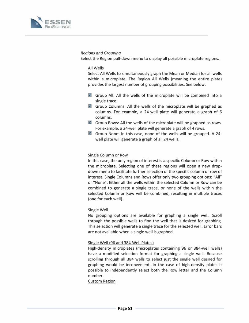
Page 51
Regions and Grouping Select the Region pull-down menu to display all possible microplate regions.
All Wells Select All Wells to simultaneously graph the Mean or Median for all wells within a microplate. The Region All Wells (meaning the entire plate) provides the largest number of grouping possibilities. See below:
Group All: All the wells of the microplate will be combined into a
single trace. Group Columns: All the wells of the microplate will be graphed as
columns. For example, a 24-well plate will generate a graph of 6 columns.
Group Rows: All the wells of the microplate will be graphed as rows. For example, a 24-well plate will generate a graph of 4 rows.
Group None: In this case, none of the wells will be grouped. A 24-well plate will generate a graph of all 24 wells.
Single Column or Row In this case, the only region of interest is a specific Column or Row within the microplate. Selecting one of these regions will open a new drop-down menu to facilitate further selection of the specific column or row of interest. Single Columns and Rows offer only two grouping options: “All” or “None”. Either all the wells within the selected Column or Row can be combined to generate a single trace, or none of the wells within the selected Column or Row will be combined, resulting in multiple traces (one for each well).
Single Well No grouping options are available for graphing a single well. Scroll through the possible wells to find the well that is desired for graphing. This selection will generate a single trace for the selected well. Error bars are not available when a single well is graphed.
Single Well (96 and 384-Well Plates) High-density microplates (microplates containing 96 or 384-well wells) have a modified selection format for graphing a single well. Because scrolling through all 384 wells to select just the single well desired for graphing would be inconvenient, in the case of high-density plates it possible to independently select both the Row letter and the Column number. Custom Region

Page 52
When Custom Region is selected, the vessel color will change from light orange to green, thus alerting the User that this is a special graphing Mode. When Custom Region is selected, the User can select/deselect a subset of individual wells with the mouse as desired. Normally, when a graph is generated, it is automatically assigned a Label based upon the selected Region and Statistic. Because in this case the Region is variable, it is possible for the User to assign a custom Label. If the Label box is not populated, the default Label will simply read Custom Region accompanied by the Statistic. To save a custom region for later use, click the “Save” button to the right of the Label box. The custom region will then be saved under the Region pull-down menu for the current vessel type. To delete a saved custom region, select it from the Region pull-down menu and click the “X” next to the Region box. The selected region will then appear as a Custom Region, giving the option to edit it or permanently delete it (by choosing a different saved region). NOTE: If a plate map is associated with a vessel (microplates only), any Region created in the Plate Map Editor will be available for graphing. To create a plate map or assign regions, see Section 7.9.
Graphing Flasks and Dishes Flasks and Dishes contain only two possible regions:
All Sectors Single Sector
Region All Sectors If All Sectors are selected, the graphs can be viewed with or without error bars, and the error bars will represent the inter-sector Mean or Median as selected in the Statistic drop-down menu.
All: All the sectors within the flask will be combined into a single trace. None: any of the sectors will be grouped. No error bars are available for
graphs of single sectors. Region Single Sector If the Region Single Sector is selected, a new drop-down menu will appear. Choose the desired sector for graphing. Error bars are not available for graphs of a single sector.

Page 53
Graph/Export Histograms of Processed Jobs It is possible to generate histograms from both Phase-contrast and fluorescent data (see Figure 20). Histograms can only be generated for a single time point, so select Single Time instead of Time Range and then select the Histogram radio button. If the Histogram radio button is selected without first choosing Single Time, the selection will automatically be reset from Time Range to Single Time.
Metrics available for Histograms are based on the Analysis Job Performed:
Basic Analyzer: Phase Object Area
Fluorescent Object Area Fluorescent Object Mean Intensity Fluorescent Object Integrated Intensity
Angiogenesis: Network Area Network Length Tube Width Uniformity Nucleus Area Nucleus Mean Intensity Nucleus Integrated Intensity
Migration/Invasion: Wound Object Area
NeuroTrack™: Cell Body Cluster Area Nucleus Area Nucleus Mean Intensity Nucleus Integrated Intensity
These same Metrics are available for Time Plots, except that in the case of Time Plots, the plot represents average values over time. Histograms display the distribution of the Metric at a single time point over the designated spatial grouping. As for Time Plots, Histogram spatial distribution can be anything from a single image to every scanned image. To customize your Histogram, press the “Histogram Bin Settings” button. A new window will open allowing the User to adjust the Min/Max Values of the x-axis as well as the Bin Count. The software will assign recommended settings based upon the data, but it is possible to substitute Custom values as desired. After Bin Settings have been selected, press the “Graph” button. Pressing the “Graph” button directly will generate a Histogram even if Bin settings are not viewed/adjusted first. The Histogram will simply use the settings assigned by the software. Increasing the number of Bins results in finer resolution of the distribution across the selected Metric.

Page 54
7.6.1.2 Graph Customization
Initial default labels along with other graph attributes can be personalized. Left-click twice on the graph background area and the Customization Window will appear (as shown in Figure 19). This window can be used to set a variety of graph attributes including graph style, axis, font, etc. Select the various tabs to explore all available graph-related features. Title, Subtitle, and individual well/sector names, however, CANNOT be changed using the Customization window. To assign new labels to wells or sectors, select the Edit option at the top left of the graph window. This will open the Titles and Labels window. This window provides an opportunity to change the Title and Subtitle, as well as the means to assign new well and sector labels. All default or previously set labels will appear in the Plot Labels box, while the currently highlighted label will appear below. To change a label, simply highlight the desired Plot Label with the mouse and then type the new label into the box underneath. Do not click “OK” until you are ready to close the Titles and Labels window. Clicking on the Advance button will bring up the Customization window. The Customization Window can also be accessed by double left-clicking on the graph.
Figure 20. Histogram

Page 55
7.6.1.3 Drag and Drop Alignment Settings Task Pane
The Drag and Drop Alignment Settings can be visualized by opening the Tasks Pane at the bottom of the Graph Window. Click on the arrow on the blue bar at the bottom of the Graph Window to open or close the Drag and Drop Alignment Tasks Pane.
7.6.1.4 Dragging and Dropping Graphs
There are two different circumstances under which graphs can be dragged and dropped using the IncuCyte™ software. Dragging and Dropping Graphs within the IncuCyte™ Software (Create Plot Overlays) Under some circumstances, it will be convenient to combine traces created in separate graphs onto one single graph in order to facilitate a direct comparison. For example, the same cells were plated in two, separate flasks at the same starting confluence at the same time. How does their growth compare? Unfortunately, the mean growth curve of each flask must be generated separately, creating two, separate graphs. However, it would be optimal if both traces could be combined onto a single graph. As indicated in the drag and drop box at the bottom of the graph window, simply right-click (and hold) on the graph to be dragged, and then use the mouse to drag it onto the target graph. Release of the mouse button will cause the graph to be dropped. The new graph still contains the title from the original, Growth Curve for vessel 1; however, it now contains two traces labeled as vesel 1 and vessel 2. If only a single trace (for example, a single well from a 12-well plate) needs to be dragged and dropped, then it (the desired well) must be graphed alone and dragged and dropped individually. Alternatively, if the entire graph is dragged and dropped, individual traces can be deleted. To drag and drop graphs onto each other within the IncuCyte™ software, be sure that the Graph on Graph selection is chosen from the Drag and Drop pull-down menu. If a graph overlay is attempted with the wrong Drag and Drop selection, a window will appear indicating that the overlay cannot occur. There are 3 commonly-made errors that can prevent creating a graph overlay from occurring. If you are not able to drag your graph, be sure that:
The correct Drag and Drop option is selected. The right mouse button is selected and not the left. You are not trying to drag the same graph onto itself.
Dragging and Dropping Graphs from the IncuCyte™ Software into Other Software Packages

Page 56
It is also possible to drag and drop a graph created within the IncuCyte™ software directly into a Word® document, EXCEL® file, PowerPoint® file or e-mail. In these cases, the graph can be dragged as either the raw data or the image. To drag the image into Word®, select Drag and Drop Image to Word or Outlook. To drag the graph image into EXCEL®, PowerPoint® or email, select Drag and Drop Image to Other Document. To drag the raw data from the graph, select Drag and Drop Raw Data to Document. If the graph is dragged as Raw Data into EXCEL®, the data will appear neatly within the spreadsheet cells. If the raw data are dragged into Word®, they will appear within columns.
The format in which the data will be dragged and dropped into the target software will be determined by the format in which the graph was created - for example, sorted by column vs. row.
SUMMARY:
To drag one plot onto another (within the IncuCyte™ graphing software) select Drag and Drop as Graph on Graph.
To drag the graph image into MS Word® or MS Outlook®, select Drag and Drop as Image to Word or Outlook.
To drag and drop the image into other software programs, select Drag and Drop as Image to Other Document.
To drag and drop other raw data, select Drag and Drop Raw Data to Document.
7.6.1.5 Creating Averaged Graphs
When multiple traces are included on a single plot, either as a result of dragging or by graphing all wells/sectors, these traces can be combined to create a single, Average Graph. To do this, select the “Tools” pull-down menu from the top of the Graph window, and then select “Average Lines Together”. Select “OK” in the dialog box that appears, and a new, Average graph will be created in a new window. Note that the Average Graph function does not generate a graph with error bars.
The Average graph function can be also used to combine graphs from different vessels and/or from different days.
7.6.1.6 Preferences: Outlier Removal and Drag and Drop Auto Alignment
When generating the selected Metrics, the stringency of outlier removal can be adjusted by selecting the “Preferences” option from the top of the main IncuCyte™ screen to open the “Preferences/Outlier Removal” Window. Two features of the Preferences window will be discussed here.
Page 57
Outlier Removal
This function facilitates the increasingly stringent removal of outlying vessel data. Selecting Outlier Removal will reduce the standard deviation of the Metrics. The outlying data are selected automatically by the software according to an algorithm - points cannot be excluded manually. Select from “None” (no outlier removal), “Standard” or “Aggressive”. Whenever a graph is created, it will conform to the currently selected degree of stringency. None is the IncuCyte™ default setting, and it is recommended.
Graph Drag and Drop: Auto Alignment When graphs are dragged and dropped to create a plot overlay, they can be set to automatically align at a specific point on the Y-axis. Select the “Drag and Drop: Auto Align at Y-Value when Drag and Drop occurs” check box in the Preferences Window.
The Drag and Drop Alignment selection (selected or un-selected) chosen via the Preferences window will apply to all graph overlays, but the numerical value at which alignment occurs MUST be set using the Graph Window. To select the numerical value for alignment, use the “Auto Alignment” tab at the bottom of the Graph Window, and choose the value at which alignment will occur (the default value is 22). Whatever alignment value is set under this tab will apply to all future graph overlays. To change the value, select a new value, and then press “Apply”. See Auto Alignment under Other Graph Features (section 7.6.1.7) for more information.
7.6.1.7 Other Graph Features
Error Bars When multiple wells or sectors are combined to generate a single trace, Error Bars can be added that represent the standard deviation between the wells or sectors. Standard Error and Standard Deviation Error Bars are available. The Standard Error Bars are the default selection. To change or remove Error Bars select the “View” drop down menu from the top of the Graph window. When Error Bars are chosen, then all graphs generated subsequent to that time will automatically be assigned Error Bars. Deselecting the Error Bars will eliminate all Error Bars from subsequent graphs.

Page 58
Calendar Mode At the bottom, right corner of the graph is the Calendar Mode check box. If the Calendar Mode box is selected, the x-axis of the graph will be displayed as year, month, day and time. If Calendar Mode is NOT selected, the x-axis will be displayed in units of hours. When should Calendar Mode be used? If multiple graphs were created over the same time period, they can be dragged to create overlays in the Calendar Mode setting. This overlay facilitates a comparison of cell growth in absolute time. However, what if the same experiment was performed on different days? In this case, if both graphs are dragged together and then displayed in Calendar Mode, they will not overlap at all because they have no dates/times in common. To display these graphs properly overlapped, view the graph overlay with the Calendar Mode button NOT checked. Now, both graphs will be displayed as confluence relative to hours, irrespective of the specific days and times, and they will be overlapped. Auto Alignment At the bottom of the Graph Window, find the “Auto Alignment” tab. This tab can always be opened, but the Auto Alignment function is only active when the Calendar Mode button is NOT checked. When the IncuCyte™ software is first opened, this value will be set to the default number, 22. However, if the value is changed from this default, the new value will be displayed until it is changed again by the User, even if the program is closed and then opened again at a later date. If the “Auto Align” button is checked, then whenever graph overlays are generated by dragging, they will be aligned at this set value. When multiple traces are included on a single graph in Calendar Mode, their relative positions are constrained by the absolute times and dates of each point within the graph. However, when Calendar Mode is no longer checked, and the traces are displayed merely as confluence relative to hours of growth, individual traces can be aligned with each other according to a specific, selected percent confluence. If an alignment value is set that is outside the range of one or more traces, then the program cannot generate an accurate alignment. To set a new Auto Alignment value, scroll through the values in the alignment box or simply type in a new value. Then press, “Reset” or hit “Enter” on the keyboard.
Page 59
Another useful application of the Auto-Alignment function is the comparison of multiple traces at different stages of growth.
Manual Alignment/Deletion
This function enables manual alignment or deletion of each, individual trace on a graph. When the “Manual Alignment” tab is selected, the graph will initially be aligned at the value set in the Auto Alignment box. While the Auto Alignment function is used to align all traces on a graph to the same point, Manual Alignment facilitates the alignment of individual traces upon a single graph at different points. Select each trace to be manipulated using the “Trace Selection” pull-down box to the right of the slider. The selected trace can be pulled to the left and right using the slider. Use the slider to realign all three traces on the graph. NOTE: The advantage of the Manual Alignment slider over the Auto Alignment function is that Manual Alignment facilitates alignment of individual traces one at a time; whereas, Auto Alignment resets all traces simultaneously. The Manual Alignment selection also facilitates deletion of selected traces. First, select the trace to be deleted by using the “Trace Selection” pull-down box. Now, simply click on the “Delete” button. The Delete function can be used to delete a trace from any graph containing multiple traces - not just graphs created by dragging. There are 2 circumstances under which traces from a graph CANNOT be deleted. These are:
If the graph contains only a single trace. If all the wells or sectors from a vessel are graphed simultaneously, then
the trace for the very first well or sector cannot be deleted. If all wells from a microplate are graphed simultaneously, this will be the trace for Well A1.
The above two deletion rules also hold true for the target graphs onto which plot overlays are created.
Selecting an Individual Point on the Trace Use the mouse to select an individual point on a trace. Hold the mouse over the point, and the time and date of the scan represented by that point will be displayed. Double left-click on a selected point, and it will open the Vessel View window for that scan. The Vessel View window cannot be opened by double clicking on the points in an Average Graph.

Page 60
7.6.1.8 The Graph Pull-Down Menu
Selecting the graph window pull-down menu presents three additional graph-related options. File Use the File Menu to open, save, or print a graph or to close the window.
Edit The Edit Menu provides the option to edit the graph title and labels associated with traces on the graph. View Use the View Menu to select different error measurements (standard error or standard deviation), change the y-axis to a log scale, or view filters from an analysis. Tools The Tools Menu provides options to edit how the data are viewed on the graph.
Smooth Lines Sometimes, if the data are particularly noisy, the Smooth feature might be more useful than Outlier Removal. When Smooth is selected, a new window will appear to facilitate selection of the smoothing size, i.e., the number of points over which smoothing will occur. If 3 data points are selected, then each point on the graph will be averaged using its two neighboring points. NOTE: It is important to remember that smoothing is a tool for generating cleaner curves when excessive noise prevents useful interpretation of the results. The smoothing feature should be used with discretion in order to prevent overt distortion of the data.
Estimate Rate of Change When rate of change may assist data analysis (such as with cell migration assay), this option will provide an estimated rate for each point on the graph.
Average Lines Together Create a graph showing the average of all plots on the current graph. This option can also be used to average plots from different vessels by first combining plots from different graphs using the Drag-Drop feature and then averaging the resulting graph. NOTE: Error Bars are NOT available on graphs created using the Average function. Each of these functions opens a new graph window, preserving the original.

Page 61
7.6.1.9 Zooming the Graph
Zoom Once a graph has been created, it is possible to zoom into any particular area for closer inspection. To zoom, left-click the mouse and then highlight the portion of the graph to be expanded. Release the mouse to see the Zoomed portion of the graph. Undo Zoom To reverse the zooming:
Right-click on the expanded graph. A menu will appear. Select Undo Zoom from the menu, and the graph will return to its full-size format.
Type the character “Z” on the keyboard.
7.6.2 Microplate Graphing
The Microplate Graphing selection provides another option for graphing all experiments conducted in a microplate format. Using the Microplate Graphing function, users can easily graph all wells individually in high or low density microplate (refer to Figure 21). Unless selected otherwise, the Microplate Graphing color scheme directly mirrors the information in the Plate Map editor. Furthermore, Microplate graphing can be customized using the Menu options. These options include:
Editing Titles/Subtitles
Axis Range Control
Show/Hide x and y axis labels
Logarithmic y-axis scaling
S/M/L marker sizes In addition, users can export images of the Microplate Graph by selecting one of 4 different file types (PNG, TIFF, JPEG, or BMP) and selecting one of 5 different predetermined file sizes. Print and Print Preview and Drag and Drop functionality have also been added to the Microplate Graphing option.

Page 62
7.6.3 Exporting Experimental Data Data can be exported by selecting the “Export” button underneath the graph settings. Export parameters can be adjusted according to the desired Layout, Destination and Other options.
7.6.3.1 Exporting
It is possible to export the Metrics associated with a particular vessel directly to another document or to a selected file. There are a variety of options regarding the format in which the data are exported. To export vessel Metrics, select the “Export” button rather than the “Graph” button at the lower right-corner of the graphing window. Choosing the “Export” button will open a new “Export Metrics” window, in which details of the selected export format can be chosen. The scans for which data will be available for export are selected using the Time Tree in the graphing box, prior to selecting the “Export” button. The default settings are the first and last scans available for the selected vessel. The User has the option to select specific Time Ranges, by using the mouse or arrow buttons on the Time Tree. The User can select the entire time range or a subset within the range. If only the data from a single scan need to be exported, choose Single Time instead of Time Range from the drop-down menu above the Start Time radio button. If Time Range is selected, then the data set that is exported will be a continuous set within the given time span. It is NOT possible to simultaneously export data from individual, temporally discontinuous scan times. If discrete, discontinuous
Figure 21. Example Microplate Graph

Page 63
data sets are desired, then each data set must be exported individually (Single Time exports).
Which regions of the “Export Metrics” window are active are determined by selections made within the “Export Metrics” window as well as those Region and Grouping settings made prior to opening the “Export Metrics” window. For example, under the Layout heading, Show Each Scan as its Own Table can only be activated if the Group option was set to “None” during the Graph/Export Setup. The Export Metrics window is divided into 3 main sections:
Layout Destination Other Options
Each of these sections will be discussed individually.
Layout Use this section to select the overall Layout of the exported data. The data for each scan time can be displayed within a single long row or displayed as its own table.
Show Each Scan as a Single Row In this case, each scan time will be listed to the far left, and the data for each well will be displayed as a single row to the right. In Figure 22 the data are displayed as a single row. In this figure, Region: “All Wells”, Group: “None” were selected prior to opening the Export Metrics window. NOTE: Wells from which no data were obtained are omitted.
Figure 22. Single Row Export

Page 64
Show each Scan as its own Table Alternatively, the data can be displayed as a single table, one table for each scan time. This option will only be available if Group: “None” was selected in the Graph/Export setup prior to pressing the “Export” button. If each scan is displayed as its own table, the columns labels can be displayed or not by checking the corresponding check box. If data are exported in the form of a table, then wells or sectors from which no data were obtained (because they were skipped in the scan pattern) will appear as blank spaces.
Destination Choose a destination for the exported data. There are two possible destinations for exported data:
Export to Clipboard: Choose export to Clipboard to export the data directly to a new location such as EXCEL®, PowerPoint® or MS Word®. Simply select export to Clipboard, press the Export button and then navigate to the destination software. Then, choose Paste. The data should appear in the previously selected format.
Export Data to One or More Files: The data can be exported to a single file by selecting the radio button for “All Scans in One File”. For example, suppose a 96-well plate was scanned at 10 different time points. If the data are exported to a single file, when the file is opened it will contain the data for all 10 scan times.
Alternatively, the data from each time point (each scan) can be saved to a different file. In this case, select “Each Scan in a Separate File”. Continuing with the same example as above, a 96-well plate that was scanned at 10 time points will generate 10 individual files, and each file will contain the data for a single time point. To save scans to separate files, browse to a destination file and then enter a file prefix. The Preview box will be populated automatically as the File Prefix is entered. Press the “Export” button. Whether the data are exported in a single or multi-file format, the file(s) will be saved in text format with a “.txt” extension. Open the data as a text file, or open the file in an alternate software program and then save to that program as desired.
Other Options Additional options are available when exporting data:
Include Experiment Details in the Header Fill Holes in the Data with the Following Characters

Page 65
Include Error Measurements Break Data Into Individual Images
Include Experiment Details in the Header Choose this box to include export of the following additional details along with the data: the selected Metric (usually confluence), cell type, passage number, and any notes. If multiple files are exported, the additional details will appear in every file.
Fill Holes in the Data with the Following Characters It is possible to set a scan pattern that does not include all the possible wells or sectors in the vessel. If the data are exported using the Layout option: “Show each Scan as its Own Table”, the table will have empty spaces where sectors or wells were omitted from the scan pattern. Rather than leaving these spaces empty, it is possible to select characters (e.g. “BLANK”) to fill the spaces.
Include Error Measurements Use this option to include either standard error (SE) or standard deviation (SD) for each measurement. Note that SE and SD are not available for individual images, but are calculated for the selected grouping (all, rows, columns, none). When “None” is selected, error measurements are available only if there are multiple images per sector.
Break Data Into Individual Images When there are multiple images per sector, you have the option to break data down into measurements from each image.
7.6.3.2 Dragging and Dropping Metrics
It is possible to export the Metrics associated with a particular vessel directly to
another document or to a selected file directly from the Launched Analysis job
within the Vessel View.
NOTE: It is NOT possible to drag and drop a time range. Only data from a single
scan time can be dragged and dropped.
To export data displayed in the Vessel View window follow the steps specified
below;
1. Select the “Graph/Export” tab located within the Vessel View.
2. Select the “View” menu at the top of the screen and uncheck “Condensed
Metrics”.
3. Select the desired assay metric from the drop down menu to be exported.
Located next to the icon.

Page 66
4. Select the desired time from the Time Tree located at the top-left of the
screen.
5. Right-click (and hold) anywhere within the table displaying the assay metrics.
6. Use the mouse to drag it into the target software and release the mouse
button.
7.6.4 Saving and Printing Graphs Graphs can be saved or printed using the File pull-down menu at the top of the plot. If a graph has been created and saved within the IncuCyte™ software, it can ONLY be opened again through the IncuCyte™ software (using this menu selection).If the graph file is selected by another method (for example, just locating the file on the hard drive and clicking on it), it will not open. If, however, a graph is created and then saved into another software program (for example, MS Word®), it can be opened directly through that program. In this case, however, it will be a static image that cannot be manipulated.
7.7 Exporting Images and Movies
7.7.1 Exporting Images Overview The image export function is accessed through the View Vessel window by using the “Utilities” pull down menu. Images can be exported either individually or in bulk. The Image can be exported as one of twelve image types, depending upon the channel used to acquire the images:
Blended Composite using current display settings (JPEG) Phase Contrast using the current display settings (JPEG): will export an image that
maintains the brightness and contrast settings currently displayed in the Vessel View Phase Contrast Original (JPEG) Phase Contrast Original (8-bit TIFF) Green using the current display settings (JPEG) Green uncalibrated (16-bit grayscale source PNG) Green uncalibrated (16-bit lossless TIFF)* Green calibrated (32-bit raw floating-point values)* Red using the current display settings (JPEG) Red uncalibrated (16-bit grayscale source PNG) Red uncalibrated (16-bit lossless TIFF)* Red calibrated (32-bit raw floating-point values)*
The two image types identified with an asterisk might not be as common as the other types, but they should be interpreted by most image processing software packages. Users who wish to export images for presentation applications such as MS Office should avoid the less common formats.
The fluorescence intensity of the objects and/or background can change over time when generating a sequence of fluorescent images. If the User does not want these changes to

Page 67
be reflected in the images, then the “Auto-Scale” check box should be selected prior to exporting a fluorescent image set. To apply the Auto-Scale settings to exported images, the User MUST select either:
Blended Composite using CURRENT DISPLAY SETTINGS or Fluorescence (Green or Red) using CURRENT DISPLAY SETTINGS
Additional image types are available for images that have been processed. These image types can only be exported from open Analysis Jobs.
Confluence: Confluence Mask (8-bit TIFF) Object Count: Counting Color 1 Mask (8-bit TIFF) Counting Color 2 Mask (8-bit TIFF) Angiogenesis: Network Mask (8-bit TIFF) Skeleton Mask (8-bit TIFF) Migration/Invasion: Confluence Mask (8-bit TIFF) Initial Scratch Wound Mask (8-bit TIFF) Scratch Wound Mask (8-bit TIFF) NeuroTrack™: Neurite Mask (8-bit TIFF) Cell-Body Cluster Mask (8-bit TIFF)
7.7.1.1 Export Current Image (Single Image) To export only the SINGLE image that is currently displayed in the Vessel View window following the steps specified below (refer to Figure 23); 1. Select “Export Current Image…”. A new window will open.
2. Select the appropriate image type in the Export Single Image window using the Image Type drop-down menu.
3. After the image type has been selected, browse to the file destination.
4. Select either the “keep full-size image dimensions” or “Customize with image designer…” radio buttons.

Page 68
By selecting the “Keep full-size image dimensions” option, the entire image acquired at its native size is exported using the current brightness and contrast settings. Customization of the export image is available by using the “Customize with image designer…” tool. This button launches a new “Export Designer” window that allows the User to customize the cropping and zoom level as well as the option to add a legend and timestamp if desired. With the legend option, a scale bar and field of view dimensions will appear in the exported image as they do in the Vessel View.
In the “Export Designer” window, the full size image is cropped as it appears in the Vessel View window, whether viewed full-size or zoomed-in. The cropping boundaries can also be changed in the current window by clicking on and dragging the red boundary lines within the preview window. Similarly, the cropped rectangle can be moved by clicking and dragging within the current boundaries. The final size of the cropped image in pixels is displayed below the “Scaling” control. Use this control to adjust the size and resolution of the final image. As the scaling increases, the final size increases, and vice versa. This allows you to customize the final image size, which can be very convenient when exporting data for presentation formats. By increasing the scaling, you can digitally zoom in on a small cropped area. NOTE: The sizes of both the scale bar and timestamp (in pixels) are fixed and will thus appear differently depending on scaling. Experiment with the “Scaling” option to see how this affects both the timestamp and legend on the final image.
We strongly encourage you to preview your customization settings prior to export via the “Output Preview” button found in the left-hand corner of the “Export Designer” window. Once you are satisfied with the customization, click “OK” to exit the Export Designer.
5. After the image type, file destination, and optional customization has been completed, select the “Export” button.

Page 69
7.7.1.2 Export Image Set (Multiple Images) It is possible to export all or a subset of all the images obtained for a particular vessel in bulk format by selecting the “Export Movie or Image Set” from the “Utilities” pull down menu. This window displays the selected Vessel and its corresponding Time Tree (refer to Figure 24). The window is divided into two main sections: Export Time/Area Range and Save Location and Options. Note that one or more possible images from each well or sector can be selected for export. The image number in the check box refers to which image will be exported. It does NOT refer to the total number of images that will be exported. Thus, if only the checkbox for image 3 is selected, then only image 3 will be exported for each selected well/sector and/or time point. That is, only ONE image will be exported per sector or well, and that image will always be image number 3. To export all three images for each well/sector, the checkboxes for all three image numbers must be selected.
1. Select Wells/Sectors for Image Export
One or more wells/sectors can be selected for image export.
Select one or more wells/sectors by clicking on them individually with the mouse (the wells/sector chosen will be highlighted in yellow).
Select a region of the vessel by clicking and dragging with the mouse.
Figure 23. The Export Current Image Window with Export Designer Open
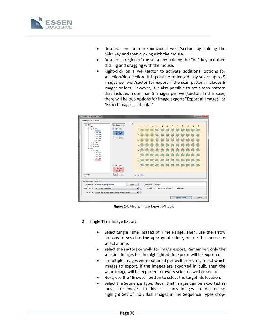
Page 70
Deselect one or more individual wells/sectors by holding the “Alt” key and then clicking with the mouse.
Deselect a region of the vessel by holding the “Alt” key and then clicking and dragging with the mouse.
Right-click on a well/sector to activate additional options for selection/deselection. It is possible to individually select up to 9 images per well/sector for export if the scan pattern includes 9 images or less. However, it is also possible to set a scan pattern that includes more than 9 images per well/sector. In this case, there will be two options for image export; “Export all Images” or “Export Image __ of Total”.
2. Single Time Image Export:
Select Single Time instead of Time Range. Then, use the arrow buttons to scroll to the appropriate time, or use the mouse to select a time.
Select the sectors or wells for image export. Remember, only the selected images for the highlighted time point will be exported.
If multiple images were obtained per well or sector, select which images to export. If the images are exported in bulk, then the same image will be exported for every selected well or sector.
Next, use the “Browse” button to select the target file location.
Select the Sequence Type. Recall that images can be exported as movies or images. In this case, only images are desired so highlight Set of Individual Images in the Sequence Types drop-
Figure 24. Movie/Image Export Window

Page 71
down menu. The movie options will still be available in this menu, but if you try to export single images as a movie, you will get an error message.
Choose Image Type
Enter the desired name into the Name Prefix box. The prefix will be automatically assigned additional time and area information that will appear in the Example box below.
Select “Export”. The “Export” button will display the total number of images (files) to be exported.
3. Time Range Image Export: Time Range Image Export is similar to Single
Time Image Export, and a review of the Single Image export instructions will be useful.
Select Time Range instead of Single Time in the drop-down menu adjacent to the Time Tree.
Use the mouse or the arrow buttons to select the scan times for export. All images including and between the selected times will be exported. NOTE: It is NOT possible to select non-consecutive times for export.
Select the desired wells/sectors and images.
Use the Browse button to choose the destination file.
Choose Sequence Type: Set of Individual Images.
Select the desired Image Type.
Enter a Name Prefix.
Click the “Export” button.
7.7.1.3 Export Image Set (Multiple Images) with Customization
Following the same setup guidelines discussed in the previous section [Export Image Set (Multiple Images)], it is possible to customize the set of exported images by customizing the image cropping and scaling and/or adding legend and timestamp information to each image. To accomplish this, the Sequence Type must be set to “Image set with customization.” Once this Sequence Type is selected, click on “Image Designer (Crop, Scale, Legend, etc)…” above the “Export” button at the bottom right of the “Movie/Image Set Export” window. A new window appears that is virtually identical to the Export Designer. As discussed in that section, the designer is used to interactively crop and scale the image and to add a legend or timestamp to each image if desired. There is an important preview tool found in the Export Designer, and we strongly recommend that the designer and previewer be used prior to launching a full image-set export with customization.

Page 72
7.7.1.4 Drag and Drop Images
It is also possible to Drag and Drop Images directly from the Vessel View Screen directly into Microsoft Word®, Outlook®, Publisher®, PowerPoint®, Excel®, or WordPad®.
To drag and drop images into other software, be sure to select the correct destination software from the “Preferences” menu on the main IncuCyte™ screen. To drag and drop an image, right-click (and hold) on the image to be dragged, and then use the mouse to drag it into the target software. Release of the mouse button will cause a new window to open. Selecting “Move here” will drop the image.
7.7.2 Exporting Movies Overview
Movies can be generated using a sequence of images within a selected time frame. A single movie can be created and exported or multiple movies can be created and exported in bulk. Because a movie by definition is comprised of a minimum of two images at consecutive time points, movies CANNOT be generated if the Single Time option is selected in the pull-down menu adjacent to the Time Tree. Movies can be created in one of two common formats (Sequence Type): Windows Media Video or Windows AVI Video. Fewer image types are available for movie export than for image export, and the descriptions are fairly self-explanatory.
Blended Composite using current display settings Phase Contrast using the current display settings Phase Contrast Original Green using the current display settings Red using the current display settings
Additional image types are available for images that have been processed. These image types can only be exported from open Analysis Jobs.
Confluence: Confluence Mask Object Count: Counting Color 1 Mask Counting Color 2 Mask Angiogenesis: Network Mask Skeleton Mask

Page 73
Migration/Invasion: Confluence Mask Initial Scratch Wound Mask Scratch Wound Mask NeuroTrack™: Neurite Mask Cell-Body Cluster Mask
7.7.2.1 Export Movie
Movie export functions are accessed through the Vessel Window by selecting the Utilities pull down menu.
To export movies follow the steps indicated below.
1. Select Time Range in the drop-down menu adjacent to the Time Tree in
the Movie/Image Set Export Window. Choose movie start and end times. The movie will include all times including and between the selected start and end times.
2. Choose the wells or sectors and the desired image numbers (as described for image export). It is possible to simultaneously export movies for all images from all wells/sectors at the same time.
3. Choose a target folder. 4. Select the Sequence Type. 5. Select Image Type 6. Select a Name Prefix. As discussed in Export Image Set (Multiple Images),
the Example box will be automatically populated. 7. If movie Sequence Type “Windows Media Video” (MWV9) or “Windows
Video AVI” is selected, a button with the text “Movie Designer (Crop, Scale, Legend, etc)…” appears above the “Export” button at the bottom right of the “Movie/Image Set Export” window.
8. Click the “Movie Designer” button and a new window appears that is
virtually identical to the Export Designer shown in Figure 23 of the “Export Current Image (Single Image)” section. As discussed in that section, the designer is used to interactively crop and scale movie frames and to add a legend or timestamp to each image if desired. If a Timestamp is added, then a timestamp that displays the corresponding time (days, hours and minutes) will appear on each frame of the movie. If Show Legend is selected, a scale bar and field of view dimensions will appear in the exported image or movie as they do in Vessel View. In

Page 74
addition to these customization options, there is also a frames-per-second parameter that can be adjusted from a minimum of 1 to a maximum of 30 frames per second. When the mouse is placed over this control, a thumbnail preview of the movie at the selected frame rate is shown as an aid.
As mentioned when discussing the Export Design window, perhaps the most important tool found in the Export Designer is launched via the “Output Preview” button in the lower left corner of the Export Designer. We strongly encourage you to preview your customization settings prior to export! The preview allows you to view a still movie frame at the exported size as well as in a full screen mode that fills your monitor. This is often important when considering the size at which the final movie will be played. Careful consideration should be given to the final size of each movie frame, which will have a huge impact (along with the number of frames) on the ultimate size of the output movie file.
9. Once you are satisfied with the customization, click “OK” to exit the
Export Designer. 10. When all the parameters have been chosen, press the “Export” button.
The Export button will indicate that number of movies (files) that will be exported under the selected conditions.
11. A new window will appear indicating the status of movie generation.
Multiple movies will be exported one immediately after the next, until all movies have been exported and compressed.
7.7.2.2 Slideshow Mode
As a quick alternative to creating a movie, click the “Slideshow” button below the time tree in Vessel View to scroll through time points of the selected image without exiting Vessel View. While in Slideshow mode, you can switch to any image in the vessel by clicking on its location at the top of the window. Also, switch to the “Graph/Export” tab to view changes in any selected metric over time. To change the speed at which IncuCyte™ cycles through images, click on the Preferences Menu at the top of the main IncuCyte™ screen.
7.8 Archiving Vessel image data, plate maps, analysis jobs and all associated data are stored on the IncuCyte™ controller. While the ≈10TB of controller hard drive space is sufficient for retaining a significant amount of data, users will eventually be required to clear space in order to continue acquiring and processing data. All vessel information can be “backed up” through a process called

Page 75
The archiving process copies the selected data from the controller to a new location. Data is not deleted from the IncuCyte controller as part of the archiving process. Once archiving has completed successfully (without errors), the original Vessel data should be deleted from the controller to clear hard drive space for future scans.
Once deleted, Vessels CANNOT be retrieved. Image data contained within archives CANNOT be re-analyzed.
archiving. Once vessels have been archived, they should be deleted from the IncuCyte controller in order to free hard drive space for future scans.
Archiving is a data management tool used to keep historical records of your vessels. Important vessels that have been fully analyzed should be archived for emergency back-up purposes. Importantly, image data contained within archives cannot be re-analyzed. While regular archiving is essential for data management, it is recommended that vessels remain on the controller as long as they are being actively evaluated.
7.8.1 Archiving Vessels
To initiate archiving, select the Archives option located on the left side task list. Once selected, the “Create New Archive” table is active, displaying all vessels available for archiving. Users can search the entire Archiving Vessels table using the “Find” field or within individual columns. (Refer to 7.4.1.2 for details on the searching tools within the IncuCyte™ ZOOM software).
Important concepts to remember while creating an archive are listed below:
Due to the volume of data involved, archives are more likely to be written
successfully when the archive size is kept small. Essen BioScience recommends
archiving data on a monthly basis or more frequently.
Smaller archives are less likely to be interrupted by system reboots, logoffs, Windows
updates, or network interruptions when archiving to “My Computer” (see below).
A small archive is more transportable.
Archives contain ONLY vessel images and their associated analysis jobs. Image
Collections and Processing Definitions CANNOT be archived.
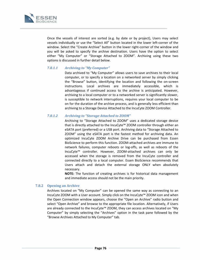
Page 76
Once the vessels of interest are sorted (e.g. by date or by project), Users may select vessels individually or use the “Select All” button located in the lower left-corner of the window. Select the “Create Archive” button in the lower right-corner of the window and you will be asked to specify the archive destination. Users have the option to select either “My Computer” or “Storage Attached to ZOOM”. Archiving using these two options is discussed in further detail below.
7.8.1.1 Archiving to “My Computer”
Data archived to “My Computer” allows users to save archives to their local computer, or to specify a location on a networked server by simply clicking the “Browse” button, identifying the location and following the on-screen instructions. Local archives are immediately accessible, which is advantageous if continued access to the archive is anticipated. However, archiving to a local computer or to a networked server is significantly slower, is susceptible to network interruptions, requires your local computer to be on for the duration of the archive process, and is generally less efficient than archiving to a Storage Device Attached to the IncuCyte ZOOM Controller.
7.8.1.2 Archiving to “Storage Attached to ZOOM”
Archiving to “Storage Attached to ZOOM” uses a dedicated storage device that is directly attached to the IncuCyte™ ZOOM controller through either an eSATA port (preferred) or a USB port. Archiving data to “Storage Attached to ZOOM” using the eSATA port is the fastest method for archiving data. An optimized IncuCyte ZOOM Archive Drive can be purchased from Essen BioScience to perform this function. ZOOM-attached archives are immune to network failures, computer reboots or log-offs, as well as reboots of the IncuCyte™ controller. However, ZOOM-attached archives can only be accessed when the storage is removed from the IncuCyte controller and connected directly to a local computer. Essen BioScience recommends that Users attach and detach the external storage ONLY when absolutely necessary. NOTE: The function of creating archives is for historical data management and immediate access should not be the main priority.
7.8.2 Opening an Archive
Archives located on “My Computer” can be opened the same way as connecting to an IncuCyte ZOOM with a User account. Simply click on the IncuCyte™ ZOOM icon and when the Open Connection window appears, choose the “Open an Archive” radio button and select “Open Archive” and browse to the appropriate file location. Alternatively, if Users are already connected to the IncuCyte™ ZOOM, they can access archives located on “My Computer” by simply selecting the “Archives” option in the task pane followed by the “Browse Archives Attached to My Computer” tab.

Page 77
IMPORTANT: When using ZOOM-attached storage, do not routinely attach and detach the drive to and from the controller. The drive should remain connected to the IncuCyte™ ZOOM until full.
WARNING! If the ZOOM-attached storage requires removal, Users MUST check the “View Archives in Progress” tab to determine if archives are being processed or are in queue. DO NOT power off or unplug the drive while in the process of archiving.
Archives that reside on ZOOM-attached devices can be viewed through the “View Archives Attached to ZOOM” tab, but cannot be accessed. If access is desired, the ZOOM-attached storage must be removed and attached to your local computer. Prior to removal, be sure to check the “View Archives In Progress” tab to confirm that there are no active archive jobs.
7.9 Hardware
7.9.1 Selecting and Placing Trays Tissue culture vessels are held within the IncuCyte™ drawer in trays. The IncuCyte™ drawer can hold a maximum of three trays, and each tray will hold different numbers of vessels depending on the tray type. A summary of all available compatible vessels and trays can be found at http://www.essenbioscience.com/support.html, under the document titled “IncuCyte™ Supported Vessel List”. The IncuCyte™ can be configured with any combination of trays and vessels from this list. While the document contains all vessel types and trays available at the time this software version was released, it is likely that new vessels and trays will be added to the list as they appear on the market and as customer demand dictates. Tray and vessel database update files are obtained by request from support (refer to Customer Support contacts listed in Section 2.3) and will be delivered as a zip archive along with database update instructions via e-mail. In order to further facilitate tray selection, each tray will have its Tray Type number stamped on the bottom portion of the tray. Additionally, the shape of each tray will be displayed when a vessel is added to the schedule.
All trays need to be placed into the IncuCyte™ ZOOM drawer in the proper orientation. To ensure proper orientation, each tray contains three Alignment Windows at its outer perimeter: one top left, one top right, one bottom right. In Figure 25 the Alignment Windows are indicated by arrows.

Page 78
The 3 tray Alignment Windows fit over 3 posts in the corresponding locations within the IncuCyte™ drawer. When placing trays into the drawer, make sure that the drawer Alignment Posts pass through the tray Alignment Windows (see Figure 26). The tray should sit very flat, and the posts should prevent any lateral movement.
Figure 25. Microplate Tray showing Alignment Windows
Figure 26. Tray Placement
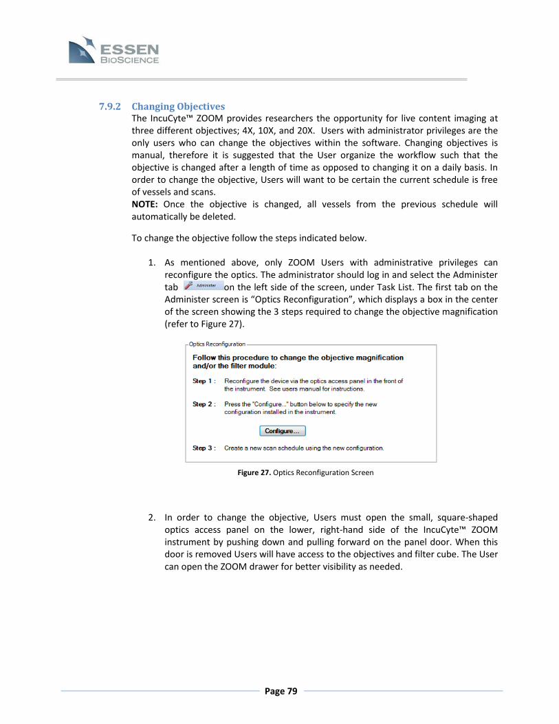
Page 79
7.9.2 Changing Objectives The IncuCyte™ ZOOM provides researchers the opportunity for live content imaging at three different objectives; 4X, 10X, and 20X. Users with administrator privileges are the only users who can change the objectives within the software. Changing objectives is manual, therefore it is suggested that the User organize the workflow such that the objective is changed after a length of time as opposed to changing it on a daily basis. In order to change the objective, Users will want to be certain the current schedule is free of vessels and scans. NOTE: Once the objective is changed, all vessels from the previous schedule will automatically be deleted.
To change the objective follow the steps indicated below.
1. As mentioned above, only ZOOM Users with administrative privileges can reconfigure the optics. The administrator should log in and select the Administer tab on the left side of the screen, under Task List. The first tab on the Administer screen is “Optics Reconfiguration”, which displays a box in the center of the screen showing the 3 steps required to change the objective magnification (refer to Figure 27).
2. In order to change the objective, Users must open the small, square-shaped
optics access panel on the lower, right-hand side of the IncuCyte™ ZOOM instrument by pushing down and pulling forward on the panel door. When this door is removed Users will have access to the objectives and filter cube. The User can open the ZOOM drawer for better visibility as needed.
Figure 27. Optics Reconfiguration Screen
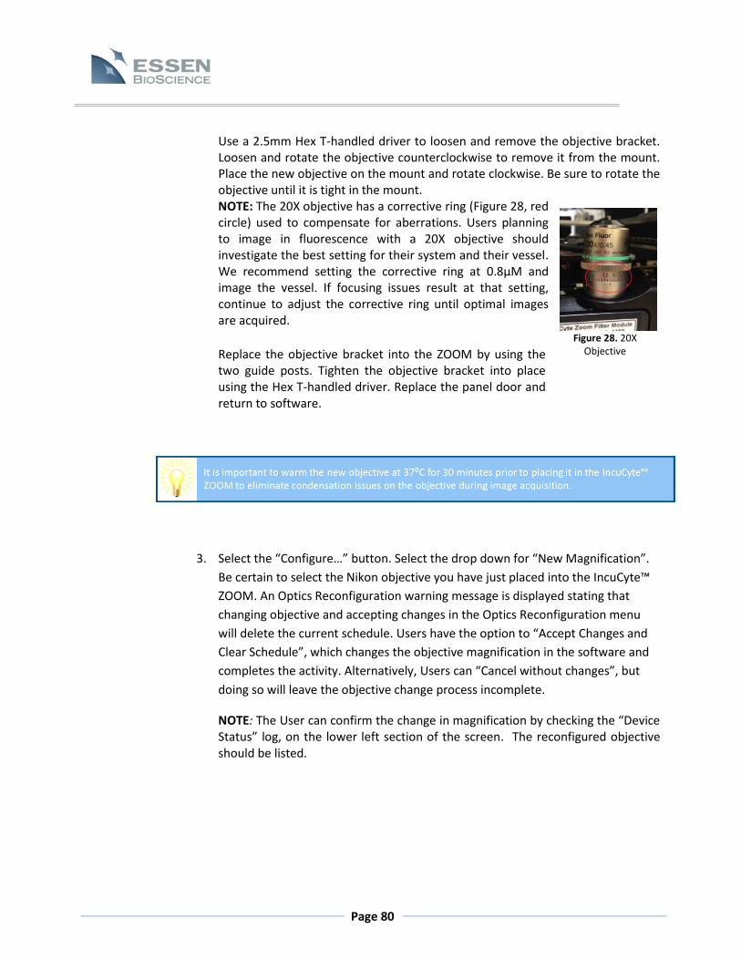
Page 80
Use a 2.5mm Hex T-handled driver to loosen and remove the objective bracket. Loosen and rotate the objective counterclockwise to remove it from the mount. Place the new objective on the mount and rotate clockwise. Be sure to rotate the objective until it is tight in the mount. NOTE: The 20X objective has a corrective ring (Figure 28, red circle) used to compensate for aberrations. Users planning to image in fluorescence with a 20X objective should investigate the best setting for their system and their vessel. We recommend setting the corrective ring at 0.8µM and image the vessel. If focusing issues result at that setting, continue to adjust the corrective ring until optimal images are acquired.
Replace the objective bracket into the ZOOM by using the two guide posts. Tighten the objective bracket into place using the Hex T-handled driver. Replace the panel door and return to software.
3. Select the “Configure…” button. Select the drop down for “New Magnification”.
Be certain to select the Nikon objective you have just placed into the IncuCyte™
ZOOM. An Optics Reconfiguration warning message is displayed stating that
changing objective and accepting changes in the Optics Reconfiguration menu
will delete the current schedule. Users have the option to “Accept Changes and
Clear Schedule”, which changes the objective magnification in the software and
completes the activity. Alternatively, Users can “Cancel without changes”, but
doing so will leave the objective change process incomplete.
NOTE: The User can confirm the change in magnification by checking the “Device Status” log, on the lower left section of the screen. The reconfigured objective should be listed.
Figure 28. 20X Objective
Page 81
7.10 Plate Map Editor To assist in experimental design and data analysis, the IncuCyte™ ZOOM software includes a Plate Map Editor that allows the User to custom-design a plate map for any microplate-based experiment. The User may design and save a plate map at any point before or during an experiment, or after the experiment has been completed. Access to the Plate Map Editor is available from four locations:
Main IncuCyte screen: Select “Plate Map…” in the File menu at the top of the window. From this location the User may save a plate map to a file, but not to an individual vessel.
Schedule Scans screen under the Properties tab Vessel View window under the Properties tab The User may open the Plate Map Editor independently of the main IncuCyte software by
browsing for the IncuCyte GUI program group via the Windows “Start” menu in the lower left of a Windows desktop.
With the Plate Map Editor open, the default screen is set to a blank 96-well plate layout. To change the plate layout, click on the New Plate Map (blank sheet) icon on the menu bar at the top-left of the window. The Plate Map Editor supports plate layouts from 6-well to 384-well formats. Refer to for Figure 29 for an overview of the Plate Map Editor. To load a plate map already saved to a file, click on the Open (folder) icon on the menu bar and browse to the file.
Figure 29. The Plate Map Editor

Page 82
7.10.1 Selecting Wells To add “well items” (cells, compounds, etc.) to a well or grouping of wells, the desired area must first be selected on the plate layout. Left-click on a well, or click-and-drag over a group of wells, to select a specific area of the plate in which to work. Wells may be deselected in the same manner. To easily select or deselect entire rows or columns, click the row/column label along the border of the plate. Select and deselect all wells in the plate by clicking on the “All” button on the top-left of the plate. Immediately to the left of the “All” button is a “blank plate” icon that will also deselect all wells.
7.10.2 Adding Well Items Before any information can be applied to a well on the plate map, it must first be loaded into one of three lists to the left of the plate map. “Compounds” are any treatments to a well where concentrations or dilutions must be specified. “Cells” specifies type, passage, and seeding density for cells present on the plate. “Growth Conditions” are additions such as growth medium where concentrations of a reagent will not vary or need not be specified on the plate map.
7.10.2.1 Compounds 1. To add a compound to the plate map, select the “Compound” tabs then
click the “New” button below the (blank) compound list.
2. In a new window, enter a name to appear on the plate map and, optionally, a longer description to appear in the list of compounds. Additionally, select a color in which the compound will appear on the plate map; when creating a dilution of a compound, higher concentrations will appear as darker shades of the indicated color.
3. After creating a compound description, select the desired area of the plate and click “Add ___...”.
4. A new window will appear allowing the User to select a desired
concentration and, optionally, a dilution series. First, select the units in which concentration will appear by clicking the drop-down menu at the top of the window (the default setting is “mg/mL”) and enter a numerical concentration to the left. If only a single concentration is desired, click “OK” and the compound will appear on the plate map.
5. To create a dilution series, check the box next to “Create a dilution” to
activate dilution options. In the drop-down menu immediately to the right, select “divide by” or “subtract” and enter value by which to dilute. Alternatively, select “manually enter” to enter a range of concentrations separated by spaces or semicolons (1000; 300; 100; 30…). To arrange the dilution series on the plate, select the direction in which the dilution series runs by selecting a direction under “Dilute wells…” and the direction in which the replicates run. If, for example, a dilution series runs from left-to-right and the User wants the replicates to be arranged

Page 83
horizontally, a box will appear allowing the User to specify how many wells exist at each concentration (singlets, duplicates, triplicates, etc.). Once the dilution series is specified, click “OK” and the compound will appear on the plate map in the specified series.
7.10.2.2 Cells To add a cell type, select the “Cells” tab then click the “New” button. Once a region of the plate is selected, click “Add ___...” to open up a new window. Here, specify passage number and seeding density, and click “OK” to add the cell type to the plate map.
7.10.2.3 Growth Conditions Once a growth condition is specified in the list, simply click “Add ___...” to add it to the plate. Because the Growth Conditions category is used for conditions where no concentration or dilution series is specified, clicking “Add ___...” will add the condition directly to the plate with no intervening options.
7.10.2.4 Adding Multiple Well Items To sequentially add multiple items to a grouping of wells (i.e. cells, growth conditions, compounds), select the plate map icon, second-to-the-right on the top menu, that reads “Keep Current Selection After Adding to Wells”. Normally after adding an item to a well or group of wells, that grouping will automatically be deselected. With the “Keep Selection…” icon activated, the selected grouping will remain selected after addition of a well item.
7.10.2.5 Deleting/Editing Well Items from Lists Once the three lists are populated, the User may edit or delete items from the lists. Editing an item will open the same window as when adding an item to a list, only the fields in the window will already contain the information for the selected item. Edit the desired fields (Short Name, Description, Color) and hit “OK” to save the changes. To delete an item from a list, simply click on the item, hit “Delete,” and “OK”. NOTE: This action does not delete any instances of the item already added to the plate map.
7.10.2.6 Editing Well Contents Once a well or group of wells are populated, the User can edit its contents and appearance. To edit well contents, first select the desired wells by left-clicking over them, then right-click within the selected region to bring up the editing window. From here, the User can create a custom description of the selected well(s), delete items, and change the color scheme of the well(s). Alternatively, use the “Undo” and “Redo” buttons in the menu bar at the top-left of the window if a mistake is made while editing a well’s contents. In addition, text size/font/style can be changed using the font button in the menu bar.

Page 84
7.10.2.7 Creating and Using Regions Regions on a plate map allow the User to define a specific set of wells (e.g. a dilution series), which aids in graphing and exporting data from an experiment. Once defined, Regions appear in the Graph/Export window in the “Regions” drop-down list and allow graphing/exporting of a custom grouping of wells. Any replicates defined within the region are automatically detected and can be grouped by selecting “Replicates” in the Graph/Export “Group” drop-down list. For example, the User can create a region such that an entire dilution series, along with negative and positive controls, appears on the same graph without the need to drag-and-drop individual plots onto one graph. In addition, the labels on individual wells or groups of wells (“replicates”) will automatically appear in the figure legend of the graph. To create a Region on a plate map, simply select the desired area of the plate in the Plate Map Editor and click on “Save Selection as Region…” under the Regions tab on the left side of the window. Enter a name for the region and hit “OK” to save the region. To create a graph of or export data from a saved Region, go to the Graph/Export window (from an opened Job Analysis in the View Vessel window) and find the Region in the “Regions” drop-down list (Regions created from the Plate Map Editor will be highlighted in blue). Select “Replicates” from the “Group” drop-down list to view each group of replicates (e.g. a specific drug concentration) as its own plot on the graph or to arrange exported data into replicates.
7.10.2.8 Printing a Plate Map At any time during the creation of a plate map, the User may print a hard copy of the map to put in a lab notebook or for reference use while in the lab. The “Print” and “Print Preview” buttons are both found in the menu bar at the top-left of the Plate Map Editor. In addition to the plate map, the hard copy will also include any notes written in the “Plate Map Notes” section below the Well Item lists in the Plate Map Editor.
7.10.2.9 Exporting an image of the Plate Map In addition to simple print functions. Users can also export Plate Map images using the Export Plate Map button at the bottom left hand corner of the editor. This brings up a selection menu where the User can select from 4 different file formats (PNG, TIFF, JPEG, BMP) and 5 different predetermined sizes.

Page 85
Chapter 8: Special Modules and Scan Types In addition, to the Standard Basic Analyzer, special Image Processing Software Modules are available with enhanced processing features. These Modules allow Users to customize processing for migration and invasion (Scratch Wound), angiogenic tube formation (Angiogenesis), and neurite dynamics (NeuroTrack™).
The Invasion/Migration and Angiogenesis (at 10X objective) require additional scan types other than the standard scanning types used for HD phase-contrast, green channel fluorescence and red channel fluorescence imaging. Using Essen ImageLock™ plates, Users have the ability to analyze invading or migrating cells using the Scratch Wound scan type. When users want to visualize a larger, more integrated view of the angiogenic network without compromising image resolution, the Tiled Field of View (FOV) mosaic image scan type option is available when using a 10X objective. Special Modules and Scan Types are described in further detail below.
8.1 Scan Types available with Essen ImageLock™ Essen BioScience manufactures a special 24 and 96-well plate type called the Essen ImageLock™ plate. These plates facilitate very precise, repeated imaging within each well. Under standard imaging conditions, slight variations can occur in the location of imaging from one scan to the next, resulting in small jumps between frames. When very precise, repeated imaging is required – for instance, when generating a movie – use the Essen ImageLock™ plate. When utilizing an ImageLock™ plate, Users can be run either the Scratch Wound or Standard (with lock) scan type options. Because the scanning process is so precise in ImageLock™ mode, the scan length will be longer than that for a plate run in Phase-Contrast mode. The scan patterns available for the ImageLock™ 24 and 96-well plates differ from those available
for standard 24 and 96-well plates. A maximum of three images is possible per well and the scan
pattern is arranged in a straight line through the center of each well, dictated by the grid on the
bottom of the wells.
8.1.1 Standard (with Lock)
By selecting an ImageLock™ plate and running it in Standard (with lock) mode, the highest fidelity movie will be generated. When an ImageLock™ plate is selected as the vessel type , the Scan Type drop-down box located under the Scan Mode in the Scan Setup tab will include the Standard (with lock) option.
8.1.2 Scratch Wound
The grid on the bottom of the wells of an Essen ImageLock™ plate allows the IncuCyte™ ZOOM to find an exact location on the plate for imaging, which is necessary when performing migration and invasion assays using the Essen Woundmaker™. When an ImageLock™ plate is selected as the vessel type, the Scan Type drop-down box located under the Scan Mode in the Scan Setup tab will include the Scratch Wound option.

Page 86
When performing invasion and migration assays, the Scratch Wound scan type can be utilized at any of the three objectives (4X, 10X, or 20X). Additionally, a “Wide Mode” scan type is available to ensure that both boundaries of the wound are imaged. The “Wide Mode” scan type is mandatory when acquiring images using the 20X objective, is optional when using the 10X objective, and is not an available feature when scanning vessels at 4X. To utilize the “Wide Mode” scan type, select the check box located beneath the scan type in the “Scan Mode” task pane.
8.2 Cell Migration/Invasion Module The Cell Migration/Invasion Software Module is used to identify the Relative Wound Density of cells invading or migrating into a scratch created using the Essen Woundmaker™. Depending on your type of assay, the IncuCyte™ ZOOM used in conjunction with the Cell Migration/Invasion Module can measure the rate and extent of cell movement into that wound over time. In the first step of the process, the cell migration/invasion algorithm analyzes each image and assigns a well-specific wound mask that corresponds to the Initial Scratch Wound. From here a Scratch Wound Mask follows invading and migrating cells as they move into the initial wound, creating a measurement of Relative Wound Density.
8.3 Angiogenesis Analysis Module The Angiogenesis Analysis Software Module is used to identify the fluorescent signal from background in order to quantify multiple angiogenic assay metrics, such as tube length and branch formation, for each time point. In the first step of the process, the angiogenesis algorithm analyzes each fluorescent image and assigns a segmentation mask that closely resembles the in vitro network. From here, the mask can be refined and filtered to exclude non-tube forming events, specifically measuring angiogenesis over time.
8.3.1 Tiled Field of View Mosaic Imaging Mode
The Tiled Field of View (FOV) mosaic image scan type stitches together six images, from a 2 x 3 grid, to produce a larger, more integrated view of the angiogenic network (Figure 30). Because the scanning process acquires 6 images per well, the scan length will be longer than that for a plate run using the 4X objective.

Page 87
The Tiled Field of View (FOV) is available when scanning Corning 96 well plates at 10X. If a 96-well plate is selected as the vessel type, the Scan Type drop-down box located under the Scan Mode in the Scan Setup tab will include a “Tiled Field of View” option. NOTE: The 10X FOV is similar to imaging a 96-well plate with a 4X objective in standard mode.
8.4 NeuroTrackTM Module The NeuroTrack™ Module is used to identify neurite dynamics for the study of neurotoxicity, neurodegeneration, neuronal development, and differentiation. The NeuroTrack™ Module can quantify multiple label-free assay metrics such as neurite length, cell body clusters, and branch points. In the first step of the process, the NeuroTrack™ software analyzes a HD phase image of neurons by first differentiating the cell bodies from the background based on texture and/or brightness, and masks them as cell body clusters. From here, linear features are detected based on width and brightness and are masked as neurites. The segmentation mask can be refined and filtered by adjusting a few parameters to tailor the mask to the specific cell type used in the assay.
Figure 30. Diagram of Tiled Field of View

Page 88
Chapter 9: Troubleshooting The quality of images and subsequent confluence measurements obtained using the IncuCyte™ ZOOM depend on having a clear, unobstructed light path through the particular well or flask. Therefore, before use, carefully inspect the vessels selected for the experiment. The following is a list of important issues to avoid:
Vessels that have scratches on the bottom or top (lids for microplates/dishes).
Drops of media or other liquid on the outside tops/lids of vessels. If this occurs, carefully clean with ethanol and a Kimwipe.
Media hanging on the inside of tops/lids of vessels.
Condensation on top/outside of vessel.
Touching either the tops or bottoms of vessels during manipulations. Hold vessels by the sides.
Writing labels on the tops of vessels. The writing will interfere with the images. Label vessels on the sides, or on the very edges of the tops where imaging will not occur.
It is VERY IMPORTANT that all lids are tightly fastened onto the flasks. If the lids are loose, it can cause the flasks to become displaced within the tray.
Be sure all vessels are sitting COMPLETELY flat in the trays.
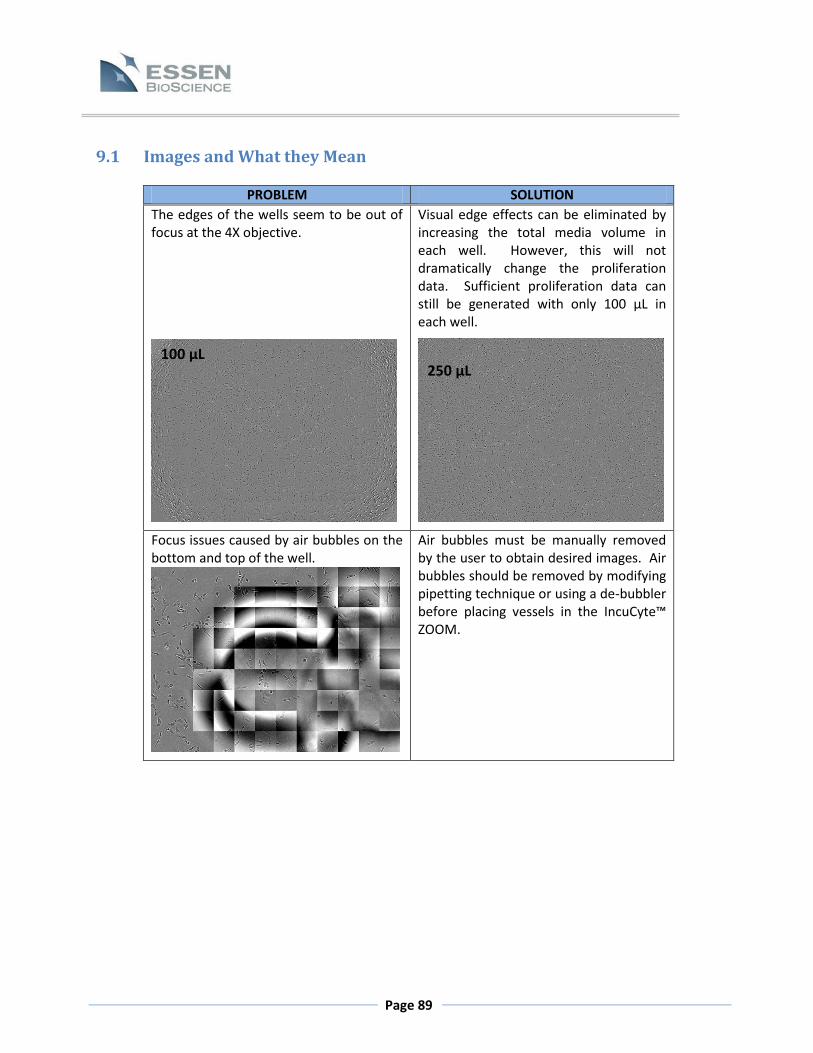
Page 89
9.1 Images and What they Mean
PROBLEM SOLUTION
The edges of the wells seem to be out of focus at the 4X objective.
Visual edge effects can be eliminated by increasing the total media volume in each well. However, this will not dramatically change the proliferation data. Sufficient proliferation data can still be generated with only 100 µL in each well.
Focus issues caused by air bubbles on the bottom and top of the well.
Air bubbles must be manually removed by the user to obtain desired images. Air bubbles should be removed by modifying pipetting technique or using a de-bubbler before placing vessels in the IncuCyte™ ZOOM.
100 µL 250 µL

Page 90
PROBLEM SOLUTION
Striations and scratches are visible on the bottom of the well.
Striations and scratches are an artifact of the vessel being used and usually will not affect the data analysis. Users should consider using a different vessel if this is a re-occurring problem or affects data analysis.
Images appear blurry.
Vibration can negatively affect image quality. The incubator that contains your IncuCyte™ ZOOM should be on a sturdy stand. If possible, try to schedule scans at times when the incubator will not be accessed, as opening and closing the incubator door can cause image blurring.
IncuCyte™ photographed condensation present on the outside, bottom of the plate instead of the cells.
Be sure to avoid condensation on the insides and outsides of all vessels prior to placing them into the IncuCyte™. Allow time for the vessel to equilibrate to the temperature of the incubator prior to initiating scans (approximately 15- 20 minutes).

Page 91
PROBLEM SOLUTION
Fluorescent cells are out of focus using the 20X objective.
Users planning to image in fluorescence with a 20X objective should investigate the best setting for their system and their vessel. Adjusting the corrective ring to 1.4µM in this case, was the optimal setting.
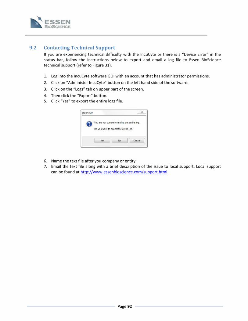
Page 92
9.2 Contacting Technical Support If you are experiencing technical difficulty with the IncuCyte or there is a “Device Error” in the status bar, follow the instructions below to export and email a log file to Essen BioScience technical support (refer to Figure 31). 1. Log into the IncuCyte software GUI with an account that has administrator permissions.
2. Click on “Administer IncuCyte” button on the left hand side of the software.
3. Click on the “Logs” tab on upper part of the screen.
4. Then click the “Export” button. 5. Click “Yes” to export the entire logs file. 6. Name the text file after you company or entity. 7. Email the text file along with a brief description of the issue to local support. Local support
can be found at http://www.essenbioscience.com/support.html

Page 93
Figure 31: The IncuCyte Log
Chapter 10: Performance Optimization The IncuCyte™ is a phase contrast microscope and as such requires an unobstructed path to the specimen from both above and below. Keep in mind the following warnings to avoid image degrading problems.
Keep vessels clean Avoid condensation Avoid bubbles Avoid media hanging on top of flasks Don’t scratch vessels Avoid writing labels on the tops of vessels Avoid touching the tops and bottoms of vessels. Handle them from the side as much as possible.

Page 94
Vibration is another factor that can negatively affect image quality. The incubator that contains your IncuCyte™ ZOOM should be on a sturdy stand. If possible, try to schedule scans at times when the incubator will not be accessed, as opening and closing the incubator door can cause image blurring even on a sturdy stand. Although it is desirable to not have large gaps in data collection, it is not necessary that the sampling be perfectly uniform. Scheduling daytime scans for just before work begins, at lunchtime, break times and again just after working hours may produce the best results. This also ensures that samples in the IncuCyte™ will be available during normal working hours in the lab. Another useful rule to follow is “don’t over-scan your samples.” We recommend keeping scan times under 45 minutes and duty cycles under 50%. As an example, 40 minute long scans scheduled every 3 hours results in a duty cycle of 22.2%. Under these conditions, any local temperature rises will typically be less than 1 degree C and relatively short lived. The IncuCyte™ is capable of collecting nearly 900 images in 30 minutes in all three channels, so another good reason to avoid such “over-scanning” is to limit the amount of data collected. This will keep the system more responsive. We have found that between 0.5 and 1 images per square centimeter is usually sufficient to characterize the growth of cells in most tissue culture vessels. For example 48 images will usually characterize a T75 flask very well. With good technique that results in uniform seeding, even fewer images can be used. Also, with some slower growing cell types scanning every 4 or even 6 hours may be sufficient.
8400-0011-C00