Aachen Institute for Advanced Study in Computational Engineering Science

Preprint: AICES-2009-8

28/January/2009

Incremental Single Shooting - A Robust Method for the

Estimation of Parameters in Dynamical Systems

C. Michalik, R. Hannemann and W. Marquardt

Financial support from the Deutsche Forschungsgemeinschaft (German Research Association) through

grant GSC 111 is gratefully acknowledged.

©C. Michalik, R. Hannemann and W. Marquardt 2009. All rights reserved

List of AICES technical reports: http://www.aices.rwth-aachen.de/preprints

Incremental Single Shooting - A Robust Method forthe Estimation of Parameters in Dynamical Systems

Claas Michalik, Ralf Hannemann, Wolfgang Marquardt∗

AVT - Process Systems Engineering, RWTH Aachen University,Turmstraße 46, D-52064Aachen, Germany.

Abstract

Estimating the parameters of a dynamical system based on measurement data is an impor-tant but complex task in industrial and scientific practice (Schittkowski, 2002). Due to itsimportance, different approaches to solve this kind of problem have been developed. Themost established ones are single shooting (Bard, 1974), multiple shooting (Bock, 1983)and full discretization techniques (Biegler, 1984). Single shooting is the most natural andsimple approach to the problem, directly combining numerical integration and optimiza-tion techniques. However, for unstable or singular systemsthe numerical integration of thedynamic model may fail. This problem is especially severe inthe framework of param-eter estimation, since the dynamic model has to be integrated many times with differentparameter estimates. Multiple shooting and full discretization aim at overcoming these de-ficiencies but suffer from other drawbacks. Therefore single shooting is still widely appliedin industry and academia. In this work we present a novel method called Incremental SingleShooting or ISS for short, which aims at overcoming the deficiencies of the classical singleshooting approach while keeping its advantages.

Key words: single shooting, parameter estimation, numerical optimization, least-squares,dynamic parameter estimation, multiple shooting

1 Introduction

Estimating parameters in dynamical systems is an importanttask in industry andacademia. Different methods are known to solve this kind of problem, the threemost established ones aresingle shooting(Bard, 1974),multiple shooting(Bock,1983) andfull discretization(Tsang et al., 1975; Biegler, 1984). All these methodspossess advantages and suffer from drawbacks. Hence, no single method turned

∗ Corresponding author. Address:Wolfgang.Marquardt@avt.rwth-aachen.de

Preprint submitted to Comp. Chem. Eng. 28 January 2009

out to be the general ’weapon of choice’ in dynamic parameter estimation. Beforepresenting our novel method (ISS) in detail, we will give a short review on classicalparameter estimation techniques and briefly discuss their advantages and disadvan-tages.

2 Established Methods for the Estimation of Parameters in Dynamic Models

We consider a class of dynamical systems described by means of differential-algebraic equations. Letx(t) ∈ R

nx be the vector of differential variables attime t ∈ [t0, tf ] , y(t) ∈ R

ny be the vector of algebraic variables andz(t) =(x(t)T ,y(t)T )T ∈ R

nz , nz = nx + ny, be the vector of differential and algebraicvariables. Letu(t) ∈ R

nu be the vector of inputs undp ∈ P be a time-invariantparameter vector which has to be estimated.P ⊂ R

np is assumed to be a compactset. We assume that consistent initial conditionsz0 and the inputsu(t) are known.Then the dynamics of the system are given by

F (x(t), z(t),u(t),p) = 0, (1)z(t0) = z0. (2)

We assume that the index of the differential-algebraic system is less than or equalto one. Lett0 < t1 < · · · < tl = tf represent a grid of points in time. Letzi, i = 1, . . . , l, be measurements of the variables at the timesti, i = 1, . . . , l.For simplicity of presentation we assume that all variablesare measured. The mea-surements are arranged in the column vector

Z :=

z1

...

zl

∈ Rl·nz , and Z(p) := Z(t1, t2, . . . , tl, z0,u;p) :=

z(t1)...

z(tl)

∈ Rl·nz ,

(3)the vector of the corresponding model predicitions, computed by the solution of theinitial value problem (1),(2).

LetVM ∈ R(l·nz)×(l·nz) be the covariance matrix of the measurements. We consider

a weighted least-squares parameter estimation problem of the form

minp∈P

(Z− Z(p))T V−1M (Z− Z(p)). (4)

2

2.1 Single Shooting

Single shooting also known as initial value approach has been introduced for opti-mal control of ODEs by Kraft (1985) and of DAEs by Cuthrell andBiegler (1987).Schittkowski (2002) employs the single shooting approach for the estimation of pa-rameters in dynamical systems. In single shooting the dynamical system is solvedby a numerical integrator.Z(p) in (4) is directly computed by numerically solv-ing an initial value problem and the vectorp ∈ P is the only degree of freedomfor the nonlinear optimizer. The advantage of single shooting is that standard DAEsolvers with sensitivity analysis capabilities and standard NLP solvers can be ap-plied. Due to the use of standard DAE solvers the grid of the state discretizationcan be adapted automatically such that the error of the states is below a prescribederror tolerance. The disadvantage is that unstable systemsare difficult or even im-possible to converge even if a good initial guess for the optimization variables isavailable. Also, single shooting can converge to several local minima due to theusually high nonlinearity of the resulting NLP. For the treatment of unstable sys-tems, multiple shooting or full discretization seem to be more favorable (Peifer andTimmer, 2007).

2.2 Direct Multiple Shooting

Multiple shooting for the direct optimization of optimal control problems1 hasbeen introduced by Bock and Plitt (1984). Roughly spoken, multiple shooting fordirect optimization is an adaption of the multiple shootingmethod for the solutionof multipoint boundary value problems to optimization. Multiple shooting for thesolution of boundary value problems has firstly been investigated by Keller (1968),Osborne (1969) and Bulirsch (1971). A state-of-the-art direct multiple shooting im-plementation is MUSCOD of Leineweber et al. (2003a,b). The basic idea of multi-ple shooting is to divide the time horizon into a number of intervals. For simplicitywe assume that the edges of the intervals coincide with the grid t0 < t1 < · · · < tl.If the dynamical system is described by a set of ordinary differential equations justthe initial values of the state variablesxi, i = 1 . . . , l, are adjoint as additionaldegrees of freedom to the optimizer. To ensure the continuity of the trajectories,junction conditions are added as equality constraints to the overall nonlinear pro-

1 Since this method is used for the direct optimization of optimal control problems it issometimes referred asdirect multiple shootingto distinguish it from the multiple shootingmethod for the solution of multipoint boundary value problems.

3

gram. We use the denotation

Z :=

x1

...

xl

∈ Rl·nz ,

and letxi(t; p), i = 1, . . . , l, be the solution of the initial value problem

xi(t) = f(xi(t),u(t),p), t ∈ [ti−1, ti], (5)xi(ti−1) = xi−1, (6)

where for notational convenience we setx0 := x0 . Then, the nonlinear program inmultiple shooting is given by

minp∈P,xi,i=1,...,l

(Z − Z)T V−1M (Z − Z) (7)

s.t. xi(ti; p) − xi = 0. (8)

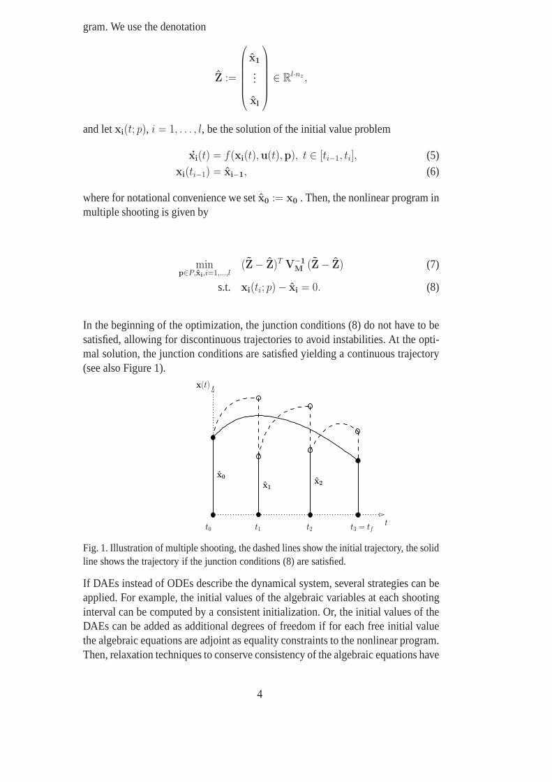
In the beginning of the optimization, the junction conditions (8) do not have to besatisfied, allowing for discontinuous trajectories to avoid instabilities. At the opti-mal solution, the junction conditions are satisfied yielding a continuous trajectory(see also Figure 1).

x0

x1x2

t0 t1 t2 t3 = tft

x(t)

Fig. 1. Illustration of multiple shooting, the dashed linesshow the initial trajectory, the solidline shows the trajectory if the junction conditions (8) aresatisfied.

If DAEs instead of ODEs describe the dynamical system, several strategies can beapplied. For example, the initial values of the algebraic variables at each shootinginterval can be computed by a consistent initialization. Or, the initial values of theDAEs can be added as additional degrees of freedom if for eachfree initial valuethe algebraic equations are adjoint as equality constraints to the nonlinear program.Then, relaxation techniques to conserve consistency of thealgebraic equations have

4

to be applied (Leineweber et al., 2003a). The advantage of the multiple shootingmethod is that a standard DAE solver for stiff systems with stepsize control can beemployed and the computer code can be parallelized in a natural way. As in singleshooting the use of stepsize control guarantees that the error of the state variablesis less than a prescribed error tolerance. On the other hand,due to the introductionof the additional degrees of freedom the size of the NLP is enlarged, especially ifthe dimension of the parameter vector is rather small compared to the dimension ofthe differential states.

2.3 Full Discretization

The full discretization method or simultaneous approach was developed by Tsanget al. (1975). In the simultaneous approach the numerical integration scheme forthe differential-algebraic equations is added as equalityconstraints to the nonlin-ear program. Orthogonal collocation is a popular choice forthe discretization ofthe differential-algebraic equations (Biegler, 1984). The choice of the discretiza-tion scheme is crucial for the success of the method. If the ”wrong” discretizationscheme is used, the nonlinear program may diverge if the discretization is refined(Kameswaran and Biegler, 2006). Usually, the full discretization leads to large-scale nonlinear programs with a sparse constraint Jacobianand a sparse Hessianof the Lagrangian. Therefore, special optimization strategies have to be applied(Cervantes et al., 2000). On the other hand, it is well known that the simulta-neous approach can successfully deal with instabilities ofthe dynamical model(Kameswaran and Biegler, 2006).

3 Incremental Single Shooting (ISS)

As discussed above, all methods presented here have some advantages and somedisadvantages. The single shooting method is widely applied since it is comparablysimple to implement. In addition, the method is available inmany modeling en-vironments and parameter estimation tools, as for instancegPROMS (ProcessSys-temsEnterprise, 2006), Aspen Custom Modeller (Aspentech,2007), JACOBIAN(Numerica Technology LLC, 2008) and Easy-Fit (Schittkowski, 2002). On theother hand, the method lacks numerical robustness (Schittkowski, 2002). Themethod presented here (ISS) is based on the single shooting approach and aimsat overcoming its deficiencies while keeping its advantages. As discussed above,the main drawback of the single shooting method is the potential infeasibility ofthe numerical integration, which might break down in the course of the integration.If the model structure under investigation is correct, thiscan happen due to a verystiff set of differential equations or – even more severe – incase of a set of differ-ential equations that is unstable or has singularities for certain parameter values.

5

Often, these problems are also caused by wrong estimates of the model parametersor initial values. However, the numerical integration typically breaks down in thecourse of the integration and not immediately at its beginning. Hence, the basicidea of ISS is to avoid the numerical integration of the wholeperiod of time, aslong as the parameter values are uncertain, by solving the parameter estimation ona reduced and successively enlarged time and data horizon. Accordingly, the periodof integration is successively increased along with the accuracy of the estimated pa-rameters until the integration is performed over the whole period of time, which isdefined by the latest available measurement information.

3.1 Algorithm of the ISS Method

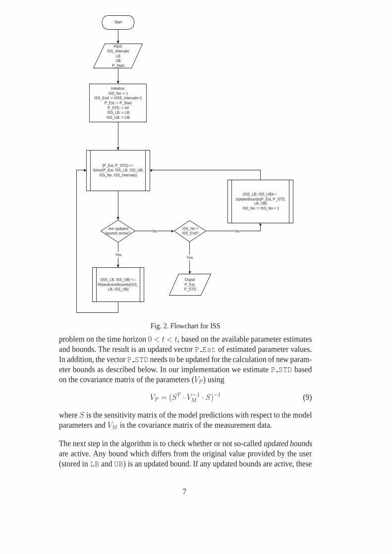
The suggested algorithm is depicted in Figure 2. The first step is mainly identicalto any other parameter estimation method. The user has to provide initial guessesfor the parameters to be estimated (P Start) along with lower (LB) and upper(UB) bounds for the parameter values2 . In addition ISS allows the user to pro-vide a vector of times(t1, t2, ..., tISS End) entitledISS Intervals correspond-ing to the integration intervals solved successively. If noISS Intervals areprovided, the intervals are determined automatically according to a heuristic de-scribed later. Hence, during thei′th ISS step, a time horizon from 0 to thei′thelement inISS Intervals is used for the parameter estimation. It is obviousthatISS Intervals should contain increasing values ending with the time ofthe latest available measurement information.

Having all these user provided information at hand, the nextstep of the algorithmis to perform some initializations. First, the counter variable (ISS No) for the ISSstep is assigned to 1 and a variable indicating the number of ISS steps (ISS End)that have to be performed is set to the number ofISS Intervals. The vector ofparameter estimates (P Est) is initialized to the user provided initial guess. Thelower bounds (ISS LB) and upper bounds (ISS UB) used during the ISS steps areinitialized to the user provided values for the parameter bounds. In addition, thestandard deviations of the estimated parameters (P STD) are initialized to infinity.

After the initialization, the first ISS problem can be solved. Here, any availablesingle shooting algorithm can be used to solve the problem with the given initialparameter guesses and parameter bounds. However, not all available measurementinformation are used. For thei′th ISS interval the set of measurement data is re-duced to those stemming from measurements taken in betweent = 0 andt = ti.Hence, the numerical integration, which is at the core of anysingle shooting algo-rithm, also only has to be performed from 0 toti.

For ISS intervali the algorithm thus starts with solving the parameter estimation

2 If no reasonable bounds are known, bounds of±∞ can be provided.

6

Start

Input: ISS_Intervals

LB UB

P_Start

Initialize: ISS_No := 1

ISS_End := #ISS_Intervals+1 P_Est := P_Start

P_STD := Inf ISS_LB := LB ISS_UB := UB

(P_Est, P_STD) <-- Solve(P_Est, ISS_LB, ISS_UB,

ISS_No, ISS_Intervals)

No Are updated

bounds active?

(ISS_LB, ISS_UB) <-- RelaxActiveBounds(ISS_

LB, ISS_UB)

Yes

ISS_No = ISS_End?

Ouput: P_Est, P_STD

Yes

(ISS_LB, ISS_UB) <-- UpdateBounds(P_Est, P_STD,

LB, UB) ISS_No := ISS_No + 1

No

Fig. 2. Flowchart for ISS

problem on the time horizon0 < t < ti based on the available parameter estimatesand bounds. The result is an updated vectorP Est of estimated parameter values.In addition, the vectorP STD needs to be updated for the calculation of new param-eter bounds as described below. In our implementation we estimateP STD basedon the covariance matrix of the parameters (VP ) using

VP = (ST· V −1

M · S)−1 (9)

whereS is the sensitivity matrix of the model predictions with respect to the modelparameters andVM is the covariance matrix of the measurement data.

The next step in the algorithm is to check whether or not so-called updated boundsare active. Any bound which differs from the original value provided by the user(stored inLB andUB) is an updated bound. If any updated bounds are active, these

7

bounds are relaxed according to

ISS UBnew = min(

ISS UBold + BRF · (ISS UBold − ISS LBold), UB)

(10)

ISS LBnew = max(

ISS LBold − BRF · (ISS UBold − ISS LBold), LB)

(11)

and the estimation problem is solved again on the same time horizon. HereBRF

is the bound relaxation factorwhich can be assigned any positive value. In ourimplementation we useBRF = 2. A higher value can reduce the necessary numberof bound relaxations and thus the computational cost but at the same time decreasesthe robustness of the algorithm.

If ISS No < ISS End the algorithm continues with the regular update of thebounds. HereISS LB andISS UB are set to the 99% confidence values of theestimated parameters3 if these values do not violate the corresponding originallower (LB) or upper bounds (UB), respectively. If the new bounds violate any orig-inal bound, the value of the original bound is used instead. In additionISS No isincreased by one and the next ISS problem is solved. The algorithm terminates ifthe last ISS interval has been solved. In this case the parameter estimates and theirstandard deviations are returned. Please note that the number of degrees of freedomfor the NLP arising from each ISS sub-problem is identical tothe single shootingcase. Hence, no additional degrees of freedom (in opposite to multiple shooting andfull discretization) are added to the NLP.

3.2 Determining the ISS intervals

The choice of ISS intervals has a high impact on the robustness and performanceof the algorithm. Various options are possible, as for instance to determine the ISSintervals based on an analysis of the system. If the numerical integration proceedsto the final time with the initially provided parameter estimates, classical SS can beapplied. If the integration breaks down attbreak, the first ISS interval can be chosento bet1 = α · tbreak, whereα is some value between 0 and 1 used to tune the robust-ness of the method. Our experience is that such methods do notwork well, since theinstabilities typically occur in the course of the estimation procedure. Frequently itis no problem to integrate the system with the initially provided parameter esti-mates, but the integration breaks down during the estimation procedure after someiterations. This is, for example, true for the second exemplary system considered(see Section 5). Here the integration is possible for all provided initial parameterguesses, but single shooting fails in 84% of the test cases during the estimationprocedure due to integration errors. Therefore, we use another strategy as default

3 Any other confidence level, as for instance the 95% confidencelevel can be used as well.

8

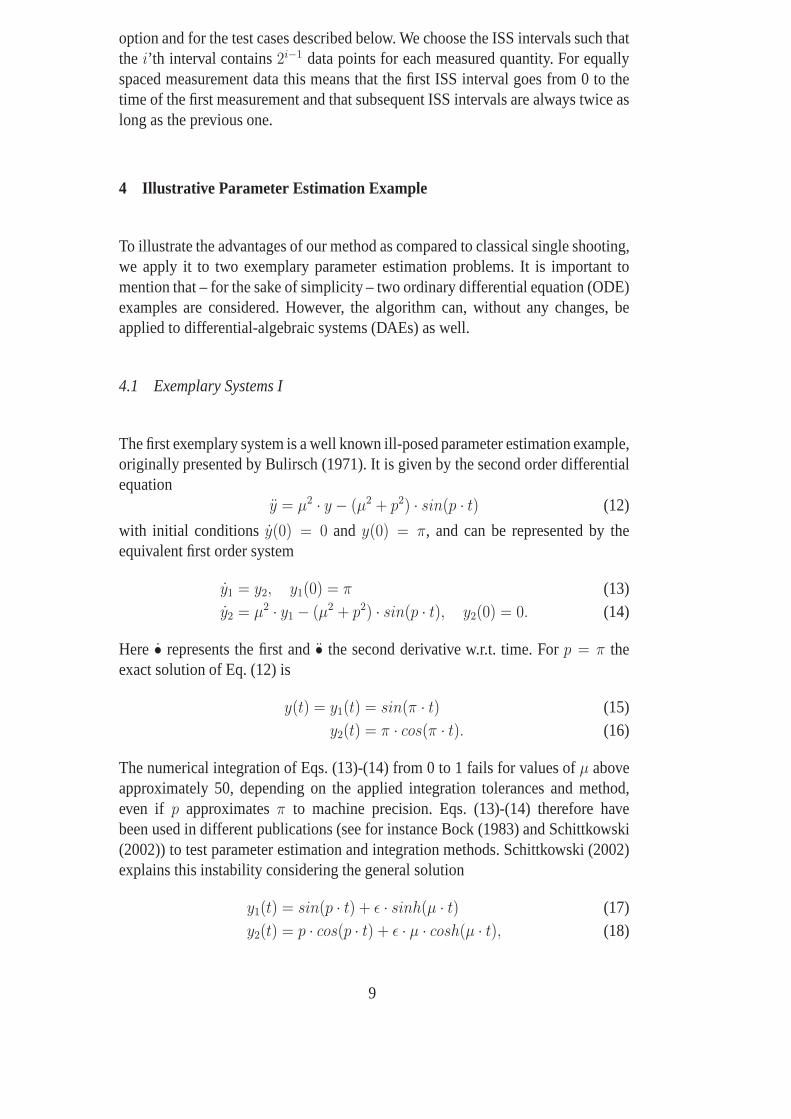
option and for the test cases described below. We choose the ISS intervals such thatthe i’th interval contains2i−1 data points for each measured quantity. For equallyspaced measurement data this means that the first ISS interval goes from 0 to thetime of the first measurement and that subsequent ISS intervals are always twice aslong as the previous one.

4 Illustrative Parameter Estimation Example

To illustrate the advantages of our method as compared to classical single shooting,we apply it to two exemplary parameter estimation problems.It is important tomention that – for the sake of simplicity – two ordinary differential equation (ODE)examples are considered. However, the algorithm can, without any changes, beapplied to differential-algebraic systems (DAEs) as well.

4.1 Exemplary Systems I

The first exemplary system is a well known ill-posed parameter estimation example,originally presented by Bulirsch (1971). It is given by the second order differentialequation

y = µ2· y − (µ2 + p2) · sin(p · t) (12)

with initial conditions y(0) = 0 and y(0) = π, and can be represented by theequivalent first order system

y1 = y2, y1(0) = π (13)y2 = µ2

· y1 − (µ2 + p2) · sin(p · t), y2(0) = 0. (14)

Here • represents the first and• the second derivative w.r.t. time. Forp = π theexact solution of Eq. (12) is

y(t) = y1(t) = sin(π · t) (15)y2(t) = π · cos(π · t). (16)

The numerical integration of Eqs. (13)-(14) from 0 to 1 failsfor values ofµ aboveapproximately 50, depending on the applied integration tolerances and method,even if p approximatesπ to machine precision. Eqs. (13)-(14) therefore havebeen used in different publications (see for instance Bock (1983) and Schittkowski(2002)) to test parameter estimation and integration methods. Schittkowski (2002)explains this instability considering the general solution

y1(t) = sin(p · t) + ǫ · sinh(µ · t) (17)y2(t) = p · cos(p · t) + ǫ · µ · cosh(µ · t), (18)

9

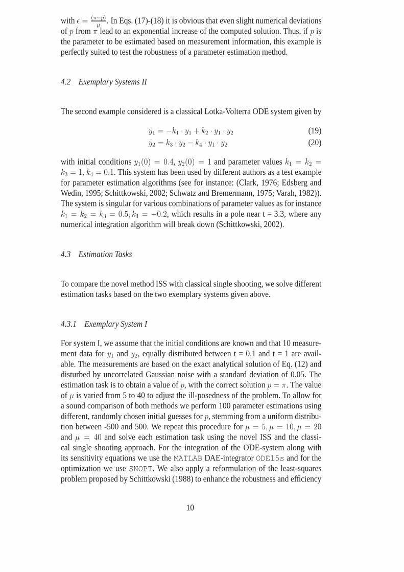
with ǫ = (π−p)µ

. In Eqs. (17)-(18) it is obvious that even slight numerical deviationsof p from π lead to an exponential increase of the computed solution. Thus, if p isthe parameter to be estimated based on measurement information, this example isperfectly suited to test the robustness of a parameter estimation method.

4.2 Exemplary Systems II

The second example considered is a classical Lotka-Volterra ODE system given by

y1 = −k1 · y1 + k2 · y1 · y2 (19)y2 = k3 · y2 − k4 · y1 · y2 (20)

with initial conditionsy1(0) = 0.4, y2(0) = 1 and parameter valuesk1 = k2 =k3 = 1, k4 = 0.1. This system has been used by different authors as a test examplefor parameter estimation algorithms (see for instance: (Clark, 1976; Edsberg andWedin, 1995; Schittkowski, 2002; Schwatz and Bremermann, 1975; Varah, 1982)).The system is singular for various combinations of parameter values as for instancek1 = k2 = k3 = 0.5, k4 = −0.2, which results in a pole near t = 3.3, where anynumerical integration algorithm will break down (Schittkowski, 2002).

4.3 Estimation Tasks

To compare the novel method ISS with classical single shooting, we solve differentestimation tasks based on the two exemplary systems given above.

4.3.1 Exemplary System I

For system I, we assume that the initial conditions are knownand that 10 measure-ment data fory1 andy2, equally distributed between t = 0.1 and t = 1 are avail-able. The measurements are based on the exact analytical solution of Eq. (12) anddisturbed by uncorrelated Gaussian noise with a standard deviation of 0.05. Theestimation task is to obtain a value ofp, with the correct solutionp = π. The valueof µ is varied from 5 to 40 to adjust the ill-posedness of the problem. To allow fora sound comparison of both methods we perform 100 parameter estimations usingdifferent, randomly chosen initial guesses forp, stemming from a uniform distribu-tion between -500 and 500. We repeat this procedure forµ = 5, µ = 10, µ = 20andµ = 40 and solve each estimation task using the novel ISS and the classi-cal single shooting approach. For the integration of the ODE-system along withits sensitivity equations we use theMATLAB DAE-integratorODE15s and for theoptimization we useSNOPT. We also apply a reformulation of the least-squaresproblem proposed by Schittkowski (1988) to enhance the robustness and efficiency

10

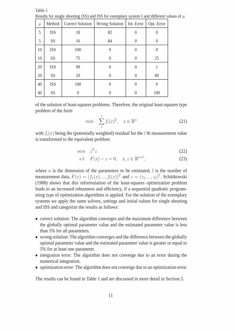
Table 1Results for single shooting (SS) and ISS for exemplary system I and different values ofµ

µ Method Correct Solution Wrong Solution Int. Error Opt. Error

5 ISS 18 82 0 0

5 SS 16 84 0 0

10 ISS 100 0 0 0

10 SS 75 0 0 25

20 ISS 99 0 0 1

20 SS 20 0 0 80

40 ISS 100 0 0 0

40 SS 0 0 0 100

of the solution of least-squares problems. Therefore, the original least-squares typeproblem of the form

minl

∑

i

fi(x)2, x ∈ Rn (21)

with fi(x) being the (potentially weighted) residual for thei’th measurement valueis transformed to the equivalent problem

min zT z (22)

s.t. F (x) − z = 0, x, z ∈ Rn+l, (23)

wheren is the dimension of the parameters to be estimated,l is the number ofmeasurement data,F (x) = (f1(x), ..., fl(x))T andz = (z1, ..., zl)

T . Schittkowski(1988) shows that this reformulation of the least-squares optimization problemleads to an increased robustness and efficiency, if a sequential quadratic program-ming type of optimization algorithms is applied. For the solution of the exemplarysystems we apply the same solvers, settings and initial values for single shootingand ISS and categorize the results as follows:

• correct solution: The algorithm converges and the maximum difference betweenthe globally optimal parameter value and the estimated parameter value is lessthan 5% for all parameters.

• wrong solution: The algorithm converges and the differencebetween the globallyoptimal parameter value and the estimated parameter value is greater or equal to5% for at least one parameter.

• integration error: The algorithm does not converge due to anerror during thenumerical integration.

• optimization error: The algorithm does not converge due to an optimization error.

The results can be found in Table 1 and are discussed in more detail in Section 5.

11

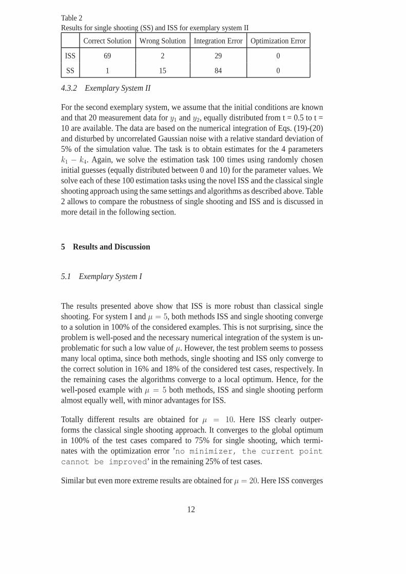
Table 2Results for single shooting (SS) and ISS for exemplary system II

Correct Solution Wrong Solution Integration Error Optimization Error

ISS 69 2 29 0

SS 1 15 84 0

4.3.2 Exemplary System II

For the second exemplary system, we assume that the initial conditions are knownand that 20 measurement data fory1 andy2, equally distributed from t = 0.5 to t =10 are available. The data are based on the numerical integration of Eqs. (19)-(20)and disturbed by uncorrelated Gaussian noise with a relative standard deviation of5% of the simulation value. The task is to obtain estimates for the 4 parametersk1 − k4. Again, we solve the estimation task 100 times using randomly choseninitial guesses (equally distributed between 0 and 10) for the parameter values. Wesolve each of these 100 estimation tasks using the novel ISS and the classical singleshooting approach using the same settings and algorithms asdescribed above. Table2 allows to compare the robustness of single shooting and ISSand is discussed inmore detail in the following section.

5 Results and Discussion

5.1 Exemplary System I

The results presented above show that ISS is more robust thanclassical singleshooting. For system I andµ = 5, both methods ISS and single shooting convergeto a solution in 100% of the considered examples. This is not surprising, since theproblem is well-posed and the necessary numerical integration of the system is un-problematic for such a low value ofµ. However, the test problem seems to possessmany local optima, since both methods, single shooting and ISS only converge tothe correct solution in 16% and 18% of the considered test cases, respectively. Inthe remaining cases the algorithms converge to a local optimum. Hence, for thewell-posed example withµ = 5 both methods, ISS and single shooting performalmost equally well, with minor advantages for ISS.

Totally different results are obtained forµ = 10. Here ISS clearly outper-forms the classical single shooting approach. It convergesto the global optimumin 100% of the test cases compared to 75% for single shooting,which termi-nates with the optimization error ’no minimizer, the current pointcannot be improved’ in the remaining 25% of test cases.

Similar but even more extreme results are obtained forµ = 20. Here ISS converges

12

to the global optimum in 99% and fails due to an optimization error in 1% of thetest cases. Single shooting on the other hand converges to the global optimum onlyin 20% of the test cases and fails due to an optimization errorin the remaining 80%of the test cases. However, the optimization error differs from the on before. Herethe optimization algorithm terminates with the error: ’General constraintscannot be satisfied accurately’. The error message is surprising atthe first glance, since the problem considered is an unconstrained least-squaresproblem. The constraints, however, appear due to the reformulation of the prob-lem described above and obviouslySNOPT is not able to find a feasible point ifsingle shooting is used.

For µ = 40 the trend seen thus far holds and ISS converges to the correctsolu-tion while single shooting fails to find the global optimum anytime. Here, singleshooting fails due to the same optimization error as before,namely: ’Generalconstraints cannot be satisfied accurately’.

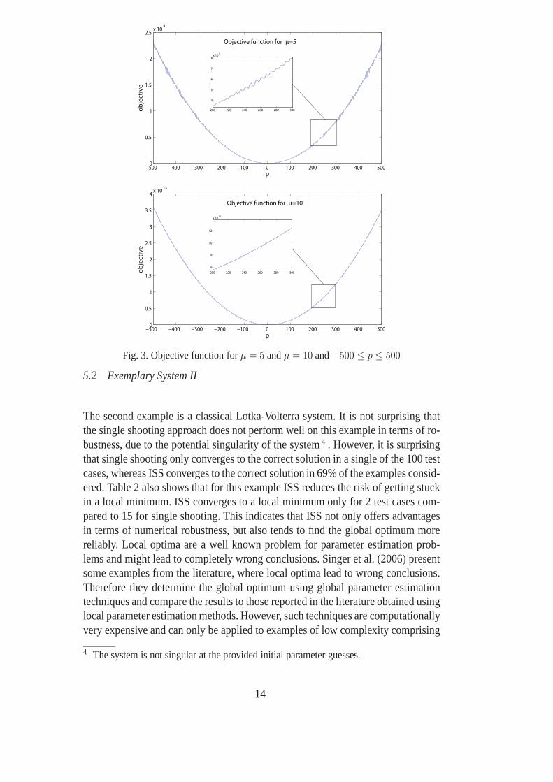
These results clearly indicate that ISS is more robust than single shooting, whichseems reasonable. However, the results are surprising, since ISS converges to theglobal optimum in 100% of the considered test cases forµ = 40 compared toonly 16% forµ = 5. Hence, the ill-posedness seems to be advantageous insteadofproblematic in this framework. This behavior can easily be explained based on ananalysis of the objective function. Using Eqs. (17) and (18)the objective functioncan be calculated as a function ofp andµ. Figure 3 shows the results for−500 ≤

p ≤ 500 andµ = 5 andµ = 10, respectively. It can be seen that the objectivefunction has many local minima forµ = 5. With increasing values forµ the ill-posedness is increasing, however, the local minima are moreand more suppressed.Hence, the optimization task is – in a way – easier to solve forhigh values ofµexcept for the numerical difficulties, which are efficientlysuppressed by ISS.

For both methods the quality of the final estimate is increasing with increasingvalues ofµ although the same, noise corrupted measurements are used for all esti-mation tasks. This is due to the sensitivity of the model prediction, which is low forsmall values ofµ. For a low sensitivity the measurement errors lead to comparablylarge errors in the estimated parameters, whereas, for a high sensitivity they leadto comparably low errors in the estimated parameters. Therefore, optimal experi-mental design strategies tend to design experiments where the model prediction ismost sensitive to the parameter values to allow an exact estimation of the parame-ters (Espie and Macchietto, 1989). However, as seen above, ahigh sensitivity cancause numerical problems if classical single shooting is applied. This emphasizesthe importance of the robustness for a parameter estimationmethod.

13

−500 −400 −300 −200 −100 0 100 200 300 400 5000

0.5

1

1.5

2

2.5x 10

9

p

ob

jec

tiv

e

Objective function for µ=5

200 220 240 260 280 300

4

5

6

7

8x 10

8

−500 −400 −300 −200 −100 0 100 200 300 400 5000

0.5

1

1.5

2

2.5

3

3.5

4x 10

13

p

ob

jec

tiv

e

Objective function for µ=10

200 220 240 260 280 300

6

8

10

12

x 1012

Fig. 3. Objective function forµ = 5 andµ = 10 and−500 ≤ p ≤ 500

5.2 Exemplary System II

The second example is a classical Lotka-Volterra system. Itis not surprising thatthe single shooting approach does not perform well on this example in terms of ro-bustness, due to the potential singularity of the system4 . However, it is surprisingthat single shooting only converges to the correct solutionin a single of the 100 testcases, whereas ISS converges to the correct solution in 69% of the examples consid-ered. Table 2 also shows that for this example ISS reduces therisk of getting stuckin a local minimum. ISS converges to a local minimum only for 2test cases com-pared to 15 for single shooting. This indicates that ISS not only offers advantagesin terms of numerical robustness, but also tends to find the global optimum morereliably. Local optima are a well known problem for parameter estimation prob-lems and might lead to completely wrong conclusions. Singeret al. (2006) presentsome examples from the literature, where local optima lead to wrong conclusions.Therefore they determine the global optimum using global parameter estimationtechniques and compare the results to those reported in the literature obtained usinglocal parameter estimation methods. However, such techniques are computationallyvery expensive and can only be applied to examples of low complexity comprising

4 The system is not singular at the provided initial parameterguesses.

14

only few parameters (Papamichail and Adjiman, 2004). Therefore local methodsare applied almost exclusively in practice and any local method that increases thechances of finding the global optimum is advantageous. Bock (1983) reports thatmultiple shooting tends to find the global optimum more reliably than single shoot-ing. ISS is similar to multiple shooting in the sense that it does not use the wholeset of available data immediately but solves multiple problems on reduced datasets. Hence, it seems reasonable that ISS can enhance the probability of finding theglobal optimum, as well. However, further investigations with different test casesare necessary to ascertain this characteristic of ISS.

The results discussed so far show that ISS is more robust thansingle shooting andcan enhance the probability of finding the global optimum. However, no informa-tion on the computational efficiency is given thus far. Let ustherefore consider theexample as described in Section 4.3 for the exemplary systemII and the initial pa-rameter guessk1 = 4.2176, k2 = 9.1574, k3 = 7.9221, k4 = 9.5949. Using theclassical single shooting approach, the system becomes singular during the sec-ond major iteration ofSNOPT and the calculation is aborted. Using ISS with thesame initial guess the correct solution is obtained after 55iterations. The iterationsalong with the optimal estimates after each ISS interval aregiven in Table 3. Itis important to mention that the number of iterations is relatively high in the firsttwo ISS intervals. This is where 70% of all iterations are performed. However, theestimates for 3 of the 4 parameters are almost optimal after the second ISS inter-val. Consequently, only a small number of iterations is necessary in the remainingISS intervals on longer time horizons. Within a total of 55 iterations the algorithmreaches the optimal estimates5 for all parameters and terminates.

The number of iterations seems to be rather high; however, considering that mostof the iterations are performed on a drastically reduced time horizon, the overallcomputational cost are quite low. Thus, in order to get an idea of the actual compu-tational cost we calculate theequivalent iteration number (Iequiv). This value rep-resents the equivalent number of iterations (∼integrations) on the full time horizonas it is carried out in single shooting iterations. For dynamic parameter estimationproblems the computational cost are usually dominated by the numerical integra-tion of the dynamic model. Therefore, theequivalent iteration number (Iequiv) de-fined as

Iequiv =1

tISS End

ISS End∑

i=1

nIterations,i · ti

can be used as a measure of the computational cost. HerenIterations,i is the numberof iteration performed in thei′th ISS step. For this exampleIequiv calculates to(11 · 0.5 + 28 · 1 + 5 · 2 + 4 · 4 + 3 · 8 + 4 · 10)÷ 10 = 12.35, which is comparablylow. Comparing the equivalent iteration number using ISS and the actual number of

5 Due to the noisy measurements some of the optimal parameter values differ from thetrue parameter values.

15

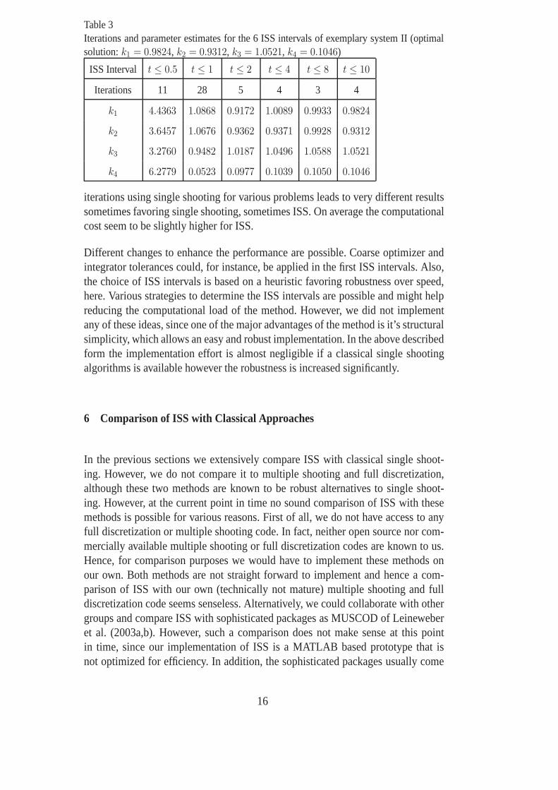
Table 3Iterations and parameter estimates for the 6 ISS intervals of exemplary system II (optimalsolution:k1 = 0.9824, k2 = 0.9312, k3 = 1.0521, k4 = 0.1046)

ISS Interval t ≤ 0.5 t ≤ 1 t ≤ 2 t ≤ 4 t ≤ 8 t ≤ 10

Iterations 11 28 5 4 3 4

k1 4.4363 1.0868 0.9172 1.0089 0.9933 0.9824

k2 3.6457 1.0676 0.9362 0.9371 0.9928 0.9312

k3 3.2760 0.9482 1.0187 1.0496 1.0588 1.0521

k4 6.2779 0.0523 0.0977 0.1039 0.1050 0.1046

iterations using single shooting for various problems leads to very different resultssometimes favoring single shooting, sometimes ISS. On average the computationalcost seem to be slightly higher for ISS.

Different changes to enhance the performance are possible.Coarse optimizer andintegrator tolerances could, for instance, be applied in the first ISS intervals. Also,the choice of ISS intervals is based on a heuristic favoring robustness over speed,here. Various strategies to determine the ISS intervals arepossible and might helpreducing the computational load of the method. However, we did not implementany of these ideas, since one of the major advantages of the method is it’s structuralsimplicity, which allows an easy and robust implementation. In the above describedform the implementation effort is almost negligible if a classical single shootingalgorithms is available however the robustness is increased significantly.

6 Comparison of ISS with Classical Approaches

In the previous sections we extensively compare ISS with classical single shoot-ing. However, we do not compare it to multiple shooting and full discretization,although these two methods are known to be robust alternatives to single shoot-ing. However, at the current point in time no sound comparison of ISS with thesemethods is possible for various reasons. First of all, we do not have access to anyfull discretization or multiple shooting code. In fact, neither open source nor com-mercially available multiple shooting or full discretization codes are known to us.Hence, for comparison purposes we would have to implement these methods onour own. Both methods are not straight forward to implement and hence a com-parison of ISS with our own (technically not mature) multiple shooting and fulldiscretization code seems senseless. Alternatively, we could collaborate with othergroups and compare ISS with sophisticated packages as MUSCOD of Leineweberet al. (2003a,b). However, such a comparison does not make sense at this pointin time, since our implementation of ISS is a MATLAB based prototype that isnot optimized for efficiency. In addition, the sophisticated packages usually come

16

with their own, tailored numerical integrators and NLP codes. Hence the compari-son would primarily test the underlying numerical integrators and NLP algorithmsinstead of the parameter estimation methods. However, we want to stress that themain goal of ISS is to offer a robust alternative for single shooting that can easilyand quickly be implemented. Such a method is desirable sincealmost all availablesoftware packages for the parameter estimation in dynamic systems rely on singleshooting, besides the drawbacks mentioned.

7 Outlook

Some ideas to increase the computational performance of thealgorithm have al-ready been presented in Section 5. Besides further improving the algorithm, futurework will focus on testing and evaluating the algorithm. Furthermore we plan toincorporate the method into the efficient large scale dynamic optimization softwarepackage DyOS (Schlegel et al., 2005), such that a sound comparison of ISS withthe major parameter estimation techniques for dynamical systems (single shoot-ing, multiple shooting and full discretization) becomes possible. In addition, differ-ent strategies to determine the ISS intervals will be implemented and compared interms of numerical robustness and computational efficiency.

8 Acknowledgements

The financial support by the theDeutsche Forschungsgemeinschaft(DFG) viacol-laborative research center 540(SFB 540) and theFonds der Chemischen Industrieis greatly appreciated.

References

Aspentech, 2007. Process and equipment model development and simulation envi-ronment, http://www.aspentech.com/products/aspen-custom-modeler.cfm.

Bard, Y., 1974. Nonlinear Parameter Estimation. Academic Press, New York.Biegler, L. T., 1984. Solution of dynamic optimization problems by successive

quadratic programming and orthogonal collocation. Comput. Chem. Eng. 8,243–248.

Bock, H. G., 1983. Recent advances in parameter identification techniques forODE. In: Deuflhard, P., Hairer, E. (Eds.), Numerical Treatment of Inverse Prob-lems in Differential and Integral Equations. Birkhauser,Boston, pp. 95–121.

Bock, H. G., Plitt, K. J., Juli 1984. A multiple shooting algorithm for direct solution

17

of optimal control problems. In: 9th IFAC World Congress Budapest. PergamonPress, pp. 242–247.

Bulirsch, R., 1971. Die Mehrzielmethode zur numerischen L¨osung von nichtlin-earen Randwertproblemen und Aufgaben der optimalen Steuerung. Tech. rep.,Carl-Cranz-Gesellschaft, Oberpfaffenhofen.

Cervantes, A. M., Wachter, A., Tutuncu, R. H., Biegler,L. T., 2000. A reducedspace interior point strategy for optimization of differential algebraic systems.Computers Chem. Eng. 24 (1), 39–51.

Clark, C., 1976. Mathematical Bioeconomics. Wiler-Interscience, New York.Cuthrell, J. E., Biegler, L. T., 1987. On the optimization ofdifferential-algebraic

process systems. AIChE Journal 33 (8), 1257–1270.Edsberg, L., Wedin, P. A., 1995. Numerical tools for parameter estimation in ODE-

systems. Optimization Methods and Software 6, 193–218.Espie, D., Macchietto, S., 1989. The optimal design of dynamic experiments.

AIChE Journal 35 (2).Kameswaran, S., Biegler, L., 2006. Simultaneous dynamic optimization strategies:

Recent advances and challenges. Computers Chem. Eng. 30 (10-12), 1560–1575.Keller, H. B., 1968. Numerical Methods for Two-Point Boundary-Value Problems.

Blaisdell Waltham, Mass.Kraft, D., 1985. On converting optimal control problems into nonlinear program-

ming problems. Computational Mathematical Programming, 261–280.Leineweber, D. B., Bauer, I., Bock, H. G., Schloder, J. P., 2003a. An efficient mul-

tiple shooting based reduced sqp strategy for large-scale dynamic process opti-mization – part I: Theoretical aspects. Computers Chem. Eng. 27 (2), 157–166.

Leineweber, D. B., Bauer, I., Bock, H. G., Schloder, J. P., 2003b. An efficient mul-tiple shooting based reduced sqp strategy for large-scale dynamic process op-timization – part II: Software aspects and applications. Computers Chem. Eng.27 (2), 167–174.

Numerica Technology LLC, 2008.JACOBIAN dynamic modeling and optimiza-tion software,http://www.numericatech.com/.

Osborne, M. R., 1969. On shooting methods for boundary valueproblems. J. Math.Anal. Appl 27, 417–433.

Papamichail, I., Adjiman, C. S., 2004. Global optimizationof dynamic systems.Computers Chem. Eng. 28, 403–415.

Peifer, M., Timmer, J., 2007. Parameter estimation in ordinary differential equa-tions for biochemical processes using the method of multiple shooting. IET SystBiol 1, 78–88.

ProcessSystemsEnterprise, 2006. gproms, modelling software,http://www.psenterprise.com/gproms/index.html.

Schittkowski, K., 1988. Solving nonlinear least squares problems by a general pur-pose sqp-method. In: K.-H. Hoffmann, J.-B. Hiriart-Urruty, C. L. J. Z. (Ed.),Trends in Mathematical Optimization. pp. 295–309.

Schittkowski, K., 2002. Numerical Data Fitting in Dynamical Systems: A PracticalIntroduction With Applications and Software. Kluwer Academic Publishers.

Schlegel, M., Stockmann, K., Binder, T., Marquardt, W., 2005. Dynamic optimiza-

18

tion using adaptive control vector parameterization. Comput. Chem. Eng. 29 (8),1731–1751.

Schwatz, J., Bremermann, H., 1975. Discussion of parameterestimation in biologi-cal modelling: Algorithms for estimation and evaluation ofthe estimates. Journalof Mathematical Biology 1 (3), 241–257.

Singer, A. B., Taylor, J. W., Barton, P. I., Green, W. H., 2006. Global dynamicoptimization for parameter estimation in chemical kinetics. Journal of PhysicalChemistry A 110 (3), 971–976.

Tsang, T. H., Himmelblau, D. M., Edgar, T. F., 1975. Optimal control via colloca-tion and nonlinear programming. Int. J. Control 21, 763–768.

Varah, J. M., 1982. A spline least squares method for numerical method for numer-ical parameter estimation in differential equations. SIAMJournal on ScientificStatistical Computing 3, 28–46.

19