Embed Size (px)
Citation preview

Incremental PageRank for Twitter Data
Using Hadoop
Ibrahim Bin AbdullahT
HE
U N I V E RS
IT
Y
OF
ED I N B U
RG
H
Master of Science
Artificial Intelligence
School of Informatics
University of Edinburgh
2010
(Graduation date: 2010)
Abstract
Twitter is a very fast growing social networking site and has millions of users.
Twitter user social relationship is based on follower concept rather that we are friend
concept and following action is not mutual between Twitter user. Twitter users
can be ranked using PageRank method as followers can be represented as social
graph and the number of followers reflects influence propagation. In this dissertation
we implemented Incremental PageRank using Hadoop MapReduce framework. We
improved the existing Incremental PageRank method based on the idea that we can
reduce the number of affected nodes that are descendants of changed nodes from going
to recalculation stage by applying threshold restriction. We named our approach as
Incremental+ method. Our experimental results show that the Incremental+ PageRank
method is scalable because we successfully applied this method to calculate PageRank
value for 1.47 billion Twitter following relations. Incremental+ method also produced
the same ranking result as other methods even though we used approximation approach
in calculating the PageRank value. The result also shows that Incremental+ method
is efficient because it reduced the number of inputs per iteration and also reduced
the number or iterations of power method. The difference in time per iteration is
statistically signigficant if compared to naïve method but the statistical result test also
shows that there is no different if compared to original Incremental PageRank method.
i

Acknowledgements
First of all, I would like to express my gratitudes towards my supervisor, Dr. Miles
Osborne for guidance and encouragement. Thank you very much also for giving me
the permission to use Hadoop Cluster and thus made this dissertation possible to work.
Next, I would like to send my warmest love for my mum in Malaysia. Thank you mum,
I love you so much. Last but not least, I would like to say thank you to my sponsor
that has granted my wish to come true. Thank you very much.
ii

Declaration
I declare that this thesis was composed by myself, that the work contained herein is
my own except where explicitly stated otherwise in the text, and that this work has not
been submitted for any other degree or professional qualification except as specified.
(Ibrahim Bin Abdullah)
iii

Contents
1 Introduction 1
2 Background 42.1 Social Relation Representation . . . . . . . . . . . . . . . . . . . . . 4
2.2 PageRank . . . . . . . . . . . . . . . . . . . . . . . . . . . . . . . . 6
2.2.1 Simplified PageRank . . . . . . . . . . . . . . . . . . . . . . 6
2.2.2 Iterative Procedure . . . . . . . . . . . . . . . . . . . . . . . 7
2.2.3 Random Surfer Model . . . . . . . . . . . . . . . . . . . . . 7
2.2.4 Damping Factor . . . . . . . . . . . . . . . . . . . . . . . . 8
2.2.5 Relation to Twitter . . . . . . . . . . . . . . . . . . . . . . . 9
2.2.6 Convergence criterion . . . . . . . . . . . . . . . . . . . . . 10
2.3 Hadoop MapReduce . . . . . . . . . . . . . . . . . . . . . . . . . . 10
2.3.1 HDFS . . . . . . . . . . . . . . . . . . . . . . . . . . . . . . 10
2.3.2 MapReduce . . . . . . . . . . . . . . . . . . . . . . . . . . 11
2.4 Related Works . . . . . . . . . . . . . . . . . . . . . . . . . . . . . . 13
3 Incremental+ PageRank 193.1 Approach Proposal . . . . . . . . . . . . . . . . . . . . . . . . . . . 19
3.2 Hypotheses . . . . . . . . . . . . . . . . . . . . . . . . . . . . . . . 20
3.2.1 First Hypothesis . . . . . . . . . . . . . . . . . . . . . . . . 20
3.2.2 Second Hypothesis . . . . . . . . . . . . . . . . . . . . . . . 20
4 Experimental Framework 214.1 Hadoop Cluster . . . . . . . . . . . . . . . . . . . . . . . . . . . . . 21
4.2 Dataset . . . . . . . . . . . . . . . . . . . . . . . . . . . . . . . . . 21
4.3 Data Preprocessing . . . . . . . . . . . . . . . . . . . . . . . . . . . 22
4.4 PageRank variable setting . . . . . . . . . . . . . . . . . . . . . . . . 23
4.5 Experiment Procedures . . . . . . . . . . . . . . . . . . . . . . . . . 23
iv

4.5.1 The Before Graph . . . . . . . . . . . . . . . . . . . . . . . 23
4.5.2 The After Graph . . . . . . . . . . . . . . . . . . . . . . . . 25
4.5.2.1 Baseline . . . . . . . . . . . . . . . . . . . . . . . 25
4.5.2.2 Incremental PageRank . . . . . . . . . . . . . . . . 25
4.5.2.3 Incremental+ PageRank . . . . . . . . . . . . . . . 29
4.6 Evaluation Methods . . . . . . . . . . . . . . . . . . . . . . . . . . . 30
4.6.1 Efficiency . . . . . . . . . . . . . . . . . . . . . . . . . . . . 30
4.6.1.1 Time cost . . . . . . . . . . . . . . . . . . . . . . 30
4.6.1.2 Workload . . . . . . . . . . . . . . . . . . . . . . 31
4.6.2 Effectiveness . . . . . . . . . . . . . . . . . . . . . . . . . . 31
4.6.2.1 Root Mean Square Error (RMSE) . . . . . . . . . 31
4.6.2.2 Kendall’s Tau coefficient . . . . . . . . . . . . . . 32
5 Experimental Evaluations 335.1 Efficiency . . . . . . . . . . . . . . . . . . . . . . . . . . . . . . . . 33
5.1.1 Time cost . . . . . . . . . . . . . . . . . . . . . . . . . . . . 33
5.1.2 Workload . . . . . . . . . . . . . . . . . . . . . . . . . . . . 37
5.2 Effectiveness . . . . . . . . . . . . . . . . . . . . . . . . . . . . . . 38
5.3 Hypotheses Testing . . . . . . . . . . . . . . . . . . . . . . . . . . . 39
5.3.1 First Hypothesis Testing . . . . . . . . . . . . . . . . . . . . 39
5.3.2 Second Hypothesis Testing . . . . . . . . . . . . . . . . . . . 43
6 Discussion 466.1 Conclusion . . . . . . . . . . . . . . . . . . . . . . . . . . . . . . . 46
6.2 Future Works . . . . . . . . . . . . . . . . . . . . . . . . . . . . . . 46
Bibliography 48
v

List of Figures
2.1 Social relation between Twitter user . . . . . . . . . . . . . . . . . . 4
2.2 Simple loop which act as cycle . . . . . . . . . . . . . . . . . . . . . 8
2.3 Dangling node . . . . . . . . . . . . . . . . . . . . . . . . . . . . . . 8
2.4 MapReduce flow. Source: [9] . . . . . . . . . . . . . . . . . . . . . . 11
2.5 MapReduce word count example application . . . . . . . . . . . . . . 12
2.6 Before graph . . . . . . . . . . . . . . . . . . . . . . . . . . . . . . 15
2.7 After graph . . . . . . . . . . . . . . . . . . . . . . . . . . . . . . . 15
2.8 Tagging the graph . . . . . . . . . . . . . . . . . . . . . . . . . . . . 15
4.1 PageRank calculation workflow using naïve method. . . . . . . . . . 23
4.2 PageRank calculation workflow using incremental method . . . . . . 25
4.3 PageRank calculation workflow using incrementa+l method . . . . . . 29
5.1 Rates of convergence . . . . . . . . . . . . . . . . . . . . . . . . . . 33
5.2 Box plot for time per iteration to calculate PageRank . . . . . . . . . 37
5.3 Normal Q-Q Plot for normality testing . . . . . . . . . . . . . . . . . 41
vi

List of Tables
2.1 Effect of d on expected number of power iterations. Source:[12] . . . 9
5.1 Percentage of iteration saved . . . . . . . . . . . . . . . . . . . . . . 34
5.2 Overhead cost for time to complete . . . . . . . . . . . . . . . . . . . 35
5.3 Ripple effect in incremental method . . . . . . . . . . . . . . . . . . 35
5.4 Descriptive statistics of time per iteration to calculate PageRank . . . 36
5.5 Dataset 1 : Number of input into recalculation stage . . . . . . . . . . 37
5.6 Comparison of sample PageRank value for naïve and Incremental+
method . . . . . . . . . . . . . . . . . . . . . . . . . . . . . . . . . 38
5.7 Root Mean Square Error . . . . . . . . . . . . . . . . . . . . . . . . 38
5.8 The Kolmogorov-Smirnov Test for normality test . . . . . . . . . . . 39
5.9 Levene Test for equal variance testing . . . . . . . . . . . . . . . . . 41
5.10 ANOVA Test result . . . . . . . . . . . . . . . . . . . . . . . . . . . 42
5.11 Tukey’s HSD test result . . . . . . . . . . . . . . . . . . . . . . . . . 43
5.12 Top 10 Twitter User Ranking . . . . . . . . . . . . . . . . . . . . . . 44
5.13 Kendall’s Tau Test result. . . . . . . . . . . . . . . . . . . . . . . . . 44
vii

List of Algorithms
2.1 Incremental PageRank algorithm by Desikan et al.. Source[6] . . . . 14
4.1 MapReduce algorithm for naïve method. . . . . . . . . . . . . . . . . 24
4.2 MapReduce algorithm for Incremental method : Part A . . . . . . . . 26
4.3 MapReduce algorithm for Incremental method: Part B . . . . . . . . 27
4.4 MapReduce algorithm for Incremental+ method . . . . . . . . . . . . 29
viii

Chapter 1
Introduction
One of the basic human needs is to interact and socialize with each other. We exchange
knowledge and information from last millennium to the next millennium. It started
from smoke signal to snail mail to telegraph and then to radio and telephone. The use
of Information and Communication Technology (ICT) has rapidly changed the way we
socialize among ourselves. Based on the recent report1 by Nielsen in August 2010 on
Internet consumer in United States of America, it shows that most of the time spent
while online is on social networking; followed by online gaming and email. Moreover,
the report result also shows that about 906 hours per month spent on social network
site such as Facebook, MySpace and Twitter.
Twitter is an online microblogging service that enables registered users to post very
short updates, comments or thoughts also known as “tweets” of up to 140 characters
[1]. The restriction of 140 character is because Twitter was initially implemented to
conform to the character limit in the Short Message System (SMS). Nowadays, users
can tweet and read tweets via SMS, web and also applications in mobile devices such
as iPhone and Google Android. Depending on the security and privacy settings, the
tweets can be publicly be read by everyone or limited to those approved follower only.
The public tweets are searchable on Twitter search or any other search engine such as
Google and Bing.
Millions of tweets tweeted daily and twitter tweets are ranging from mundane daily
life routines or important news events. For example, on November 26, 2008, reports
about the terrorist attacks in Mumbai spiked suddenly on Twitter, drawing worldwide
attention before the news media could react. The second example is when the news
1http://blog.nielsen.com/nielsenwire/online_mobile/what-americans-do-online-social-media-and-games-dominate-activity/
1

Chapter 1. Introduction 2
and pictures during Haiti earthquake in 2010 circulating in Twitter first and real time
[3]. Furthermore, users can use retweet function to spread the news. Event detection
experiments on a collection of 160 million Twitter posts show that celebrity deaths are
the fastest spreading news on Twitter [16]. The trend of utilising twitter application to
update what is happening around us has open opportunity for news media agency to
broker current breaking news.
Some user tweets spam content, some tweets are just intended for a few friend and
many are just ignored. The noisy in Twitter stream data will make it more difficult
to do event detection. In addition, because of the 140 character restriction, the URLs
shortener service to convey longer tweets such as bit.ly has been widely used but this
also subjected to be abused by virus and spam threats. Furthermore, too many junk
tweets will make the user too overwhelming to read tweets and in the the end user will
give up stop using the Twitter service. Thus, it is very important to have ways to rank
users so later we can deal with spam and spotting important tweets.
There are a few ways to rank Twitter user based on currently available information.
First, we can rank user by statistics such as the number of tweets, retweets and
frequency of updating tweets can help us to weed out spammer and non-spammer,
but this method is prone to be abused by spammer. Next, we can rank user based
on tweet contents but challenge in content-based analysis is to determine whether the
tweet content is useful or not. Finally, we can do link analysis to help us to rank the
Twitter user. In link analysis we can represent the relationship between Twitter user
and followers into graph. Based on computing the graph of followers, it should yield
information that is similar to PageRank link analysis algorithm.
PageRank hypothesis is that a web page is important if it is pointed to by other
important pages [15]. PageRank is very popular method in the web searching
community and it is usually applied to web pages and not people. So, if we apply
to Twitter domain, it means if a user has a lot of followers then the chances are they
are active and people are interested in reading the associated tweets. In addition, if that
person follows another person, then that important person propagates authority.
The latest reported data in May 2010 (based on data crawled and collected in June
2009) shows that the total user is more than 40 million and 1.47 billion relations [11].
The huge amount of data like this will need a practical and effective method to calculate
the value of PageRank. New users and users deactivation will affect the growth of
users graph. In addition, as the user keeps following and unfollow will make the graph
evolving. These two important factors will be taken into account in this dissertation.

Chapter 1. Introduction 3
PageRank calculation is based on power method which need iterative implementa-
tion. This method is very slow to reach convergence. The problem with computing
PageRank for very big graph in traditional way is we need machine with high
processing power and huge memory. Now we can use Hadoop MapReduce framework
to calculate the PageRank in parallel computation and distribute the processing and
memory usage accross cluster with cheaper machine.
In this dissertation we developed a method based on incremental PageRank method
with some modification For naming convention, Desikan et al. original incremental
method [6] will be just called Incremental method and our incremental method
with threshold will be called Incremental+ ( pronounce incremental plus). We will
explore the hypothesis that Incremental+ PageRank is better than original PageRank
on computing the ranking of Twitter user along dimension efficiency. Our second
hypothesis is Incremental+ PageRank will produce same ranking result as original
PageRank.
Our experimental results show that the Incremental+ PageRank method is scalable
because we successfully applied this method to calculate PageRank value for 1.47
billion Twitter following relations. Incremental+ method also produced the same
ranking result as other methods even though we used approximation approach in
calculating the PageRank value. The result also shows that Incremental+ method
is efficient because it reduced the number of inputs per iteration and also reduced
the number or iterations of power method. The difference in time per iteration is
statistically signigficant if compared to naïve method but the statistical result test also
shows that there is no different if compared to original Incremental PageRank method.
The report will be discussed as the following chapters:
• Chapter 2: Will discuss the background theory behind Graph Theory, PageRank
and MapReduce which form the base of the work in this thesis.
• Chapter 3: Will introduce to Incremental+ PageRank method.
• Chapter 4: Will discuss how we set up our solution and the implementation of
the framework we used to evaluate it.
• Chapter 5: Will evaluate the performance of the features we developed with
PageRank calculation methods we tried.
• Chapter 6: Will conclude the findings of the thesis and discuss future directions
that our work has highlighted.

Chapter 2
Background
In this chapter the background theories and knowledge are reviewed in order to provide
the necessary support for exploration of the subject area. Firstly we will be introduced
to some key ideas in Graph Theory such as edges list and adjacency matrix and
adjacency list. Then we will discuss the main tools for our ranking task, namely the
PageRank methods. Finally we will look at Hadoop framework which will help us to
calculate PageRank in efficient manner.
2.1 Social Relation Representation
Figure 2.1: Social relation between Twitter user
We can represent the social relation among Twitter users as an edges list. As
example in Figure 2.1 we can represent relation from node 1 to node 2 as 1 −→ 2.
4

Chapter 2. Background 5
Twitter social relation is different from webpages in term of self link or sometimes
also known as self loop. It is not possible for Twitter users to follow themselves, in
constrast to web pages, sometimes the inlinks come from the webpages itself. Twitter
is also very distinguish from MySpace and Facebook in reciprocality of social relation.
In Facebook and MySpace, user can only add a friend upon approval by the requested
user. On the other hand, the concept of follower is used in Twittersphere. Even though
there is setting for follower approval but most of the Twitter just use default setting
which is anyone can follow them. Overall, if user A follows user B does not mean B
also follows user A and reciprocality of social relation is discussed in length by Kwak
et al. in [11]. Thus, the collection of nodes in social relation in Twittersphere is a
directed graph. This directed graph can be represent as adjacency matrix as follows:
1 2 3 4 5 6 7 8
1 0 1 1 0 0 0 0 0
2 0 0 1 0 0 0 0 0
3 0 0 0 0 1 0 0 0
4 0 0 0 0 0 0 0 0
5 0 0 0 1 0 0 0 0
6 0 0 0 0 1 0 0 0
7 0 0 0 0 1 0 0 0
8 0 0 0 0 0 0 1 0
Rows in the first column of matrix mean source nodes and columns in the first
row mean targets. Value 1 is to represent if there is a link between source and target. It
shows that most of the matrix contains zero which also known as sparse matrix. Sparse
matrix like this will waste storage and computing resource especially in Twitter, the
total number of user is more than 40 millions, so we will end up with at least 40M x
40M matrix. Thus, it is better for us to represent the social relation in Figure 2.1 into
adjacency list as follows:
1: {2,3}
2: {3}
......
4: { }
......
7: {5}
8: {7}

Chapter 2. Background 6
Each number before colon in every row is the source node and numbers inside
the curley bracket represent targets. Node without any outlink like node 4 in Figure
2.1 will have empty set. The representation in adjacency list as above will greatly
reduce the amount to store and will use far less computing resources compared to
adjacency matrix. On the other hand, we should note that we will lose random access
capability.This mean we have to sequentially to read everything before we can find
what we want.
2.2 PageRank
PageRank is the link-based analysis algorithm used by Google to rank webpages was
at first present as citation ranking [15]. Another popular link-based analysis is HITS
by Kleinberg which is used by Teoma search engine later acquired by Ask.com search
engine which is based on natural language [10]. Long before PageRank, the web
graph was largely an untapped source of information[12]. Page et al. used the new
innovative way which is not to based solely on the number of inlinks but also consider
the importance of page linked to it has made PageRank a popular way to do ranking.
In a nutshell, a link from a page to another is understood as a recommendation and
status of recommender is also very important.
2.2.1 Simplified PageRank
Page et al. famous ranking formula started with a simple summation equation as in
Equation 2.1. The PageRank of node u is denoted as R(u), is the sum of the PageRanks
of all nodes pointing into node u where Bu is the set of pages pointing intou [15].
In Page et al. own word, they called Bu as backlinking. Finally Nv is the number
of outlinks from node v. The idea behind dividing R(v) with Nv can be analogy as
endorsement by Donald Trump is far better than recommendation letter by a normal
high school teacher. This is because it is hard and very rate to get endorsement by
Donald Trump compared to a high school teacher recommendation letter [12].
R(u) = ∑v∈Bu
R(v)Nv
(2.1)
Chapter 2. Background 7
2.2.2 Iterative Procedure
The problem with Equation 2.1 is that the ranking value R(v) is not known. Page et
al. use iterative procedure to overcome this problem. All node is assign with initial
equal PageRank like 1. Then rule in Equation 2.1 is successively applied, subtituting
the values of the previous iterate into R(u). This process will be repeated until the
PageRank scores will eventually converge to some final stable values. The formula
representing the iterative procedure is as in Equation 2.2. Each iteration is denoted
by value of k. k+1 means next iteration and k is previous iteration This method also
known as power method.
Rk+1(u) = ∑v∈Bu
Rk(v)Nv
(2.2)
2.2.3 Random Surfer Model
Page et al. made further adjustment to the basic model of PageRank by introducing
Random Surfer Model which is based on description of the behavior of an average
web user. According to Random Surfer Model, we can analogy that a web surfer who
bounces along randomnly following the hyperlink structure of the web. Random surfer
will arrive at a page with several outlinks and has to choose randomnly of one them
that leads to new page and this random decision process will continue indefinitely.
In the long run, the proportion of time spent on a given page is measure of the
relative importance of that page. Random surfer will repeatedly found that some
page is randomly revisited repeatedly. Pages that random surfer revisits often must
be important because they must be appointed to by other important pages.
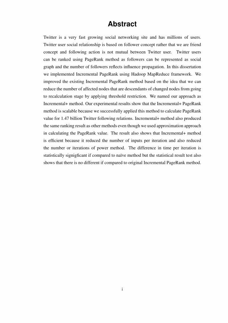
Random surfer will encounter two problems while doing the random surfing. First,
random surfer will find out it keep revisits the same cycle of node and get stuck in a
loop. Random surfer will never get a chance to visit node 5 as in Figure 2.2.
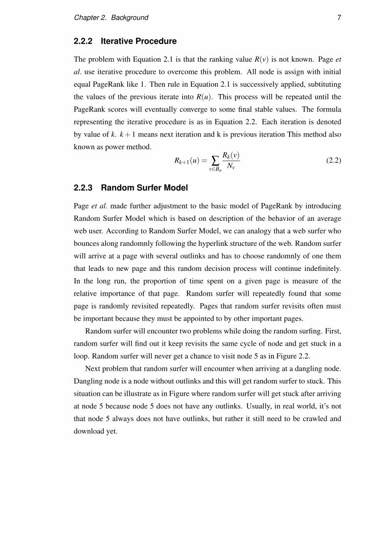
Next problem that random surfer will encounter when arriving at a dangling node.
Dangling node is a node without outlinks and this will get random surfer to stuck. This
situation can be illustrate as in Figure where random surfer will get stuck after arriving
at node 5 because node 5 does not have any outlinks. Usually, in real world, it’s not
that node 5 always does not have outlinks, but rather it still need to be crawled and
download yet.
Chapter 2. Background 8
Figure 2.2: Simple loop which act as cycle
Figure 2.3: Dangling node
2.2.4 Damping Factor
Rk+1(u) =1−d
N+d ∑
v∈Bu
Rk(v)Nv
(2.3)
In order to solve cyclic and dangling node problem, a new concept of damping
factor, constant d as in Figure 2.3 was introduced by Page et al. Damping factor is
the probability that will help random surfer at any step to continue to any another
node not in the path. It also known as teleportation factor. The damping factor is
subtracted from 1 and divided by number of nodes, N for normalisation. Different
value of damping factor have been studied by various studies [2, 4, 19], but normally
the damping factor will be set to 0.85. Suppose d = 0.85, then 85% of the time the
random surfer follows the hyperlink structure and the remaining 15% of the time the
random surfer will teleport to a new page. The convergence of PageRank calculation

Chapter 2. Background 9
also sensitive to the setting of damping factor parameter. Generally if damping factor
is set too big, it will take longer time to reach convergence but result in the site’s total
PageRank growing higher. Since there is little damping (1 - d), PageRank received
from external pages will be passed around in the system. If d value is too small it will
converge earlier but the relative PageRank will be determined by PageRank received
from external pages rather than the internal link structure [12]. We can see the effect
of d on expected number of power iteration in Table 2.1 as follows.
d Number of Iterations
.5 34
.75 81
.8 104
.85 142
.9 219
.95 449
.99 2,292
.999 23,015
Table 2.1: Effect of d on expected number of power iterations. Source:[12]
2.2.5 Relation to Twitter
How are we going to relate Random Surfer Model and damping factor in Twitter
domain? We need to change from analogy of random walking to randomnly add
new user to be followed. First method to add new user to be followed is to browse
through other user from the list either follower list or followee list The second method
is to search for specific user or we can search by trends. The third method is through
Twitter wall. Every Twitter user has a Twitter wall displaying tweets stream from
the people they followed. It really look like a river stream of tweets and sometimes
can be analogy as people writing graffiti on public toilet wall. On this wall, user can
see tweets have been retweeted and this might trigger the interest user to follow the
followee who tweets is being retweeted interestingly enough to be followed. It is like
a word of mouth concept. If our tweets is being circulated and spread, there is a high
probability that our follower will grow too.

Chapter 2. Background 10
2.2.6 Convergence criterion
The criteria for convergence or iteration termination is when the value of PageRank
is stable, but how are we going to determine it is stable? Ideally, it is stable when
sum value of difference in PageRank value reach zero, ∑‖Rk+1 − Rk‖ == 0. We
should note the absolute value of the difference between Rk+1 and Rk. In real world
implementation, social graph is full of cyclic and dangling problem, thus, it will quite
difficult to reach zero. That is why the termination criteria of iteration is setup to some
tolerance, t value ∑‖Rk+1−Rk‖ < t. For Google, 3 significant digit accuracy or t =
0.001 is used for calculating PageRank. This degree of accuracy is apparently adequate
for Google’s ranking needs. Haliwala conducted experiment to verify Google decision
for t value setting and the the result shows that the exact value of PageRank are not
important as as the correct rank ordering [8]. Rank ordering between two rankers can
be compared using a measure such as Kendall’s Tau [7].
2.3 Hadoop MapReduce
Google came out with Google File System (GFS) in order to deal massive web data and
implement MapReduce paradigm based on C++ to calculate PageRank in parallel and
distributed manner but this software is a proprietary system [5]. However, Hadoop is
a free distribution opensource framework based on Java by Apache Group and funded
by Yahoo! for running applications in reliable, scalable and distributed computing
[9]. The Hadoop framework transparently provides applications both reliability and
data motion. It implements a computational paradigm named MapReduce, where
the application is divided into many small fragments of work, each of which may
be executed or re-executed on any node in the cluster. In addition, it provides a
distributed file system (HDFS) that stores data on the compute nodes, providing very
high aggregate bandwidth across the cluster. Both MapReduce and the distributed file
system are designed so that node failures are automatically handled by the framework.
2.3.1 HDFS
HDFS stands for Hadoop Data File System and it is a cloud storage platform provides
high throughput access to application data. HDFS can handle large data, usually more
than 1 TeraBytes and even can handle PetaBytes. The most efficient data processing
pattern is write once and read many times pattern; which HDFS is built around this idea

Chapter 2. Background 11
and this made HDFS could handle streaming data access very well. Usually, a dataset
is generated or copied from source and then many analyses are performed on them over
time. Each analysis will involve a large portion, so the time to read the whole dataset
is more important than the latency in reading the first record. Hadoop also does not
require expensive and highly reliable hardware in order to run. It’s design to run on
clusters of commodity hardware and vendor independent. The chance of node failure
across the cluster is high at least for large clusters. Thus, HDFS is design to carry on
working without a noticeable interruption to the user in the face of such failure [18].
On the other hand, it is also worth to mention that HDFS is not good in the
following situation. First, applications that require low-latency access to data, in the
ten of miliseconds range, will not work well with HDFS because HDFS is optimized
for delivering high throughput of data. This may be at the expense of latency. Second,
HDFS is not suitable for lots of small files. Namenode is the master machine that serve
data file to processing machines (workers) can holds file system metadata in memory
but the limit to the number of file system is controlled by the amount of memory on the
namenode. A block takes out about 150 bytes, so if we have one million small files,
each taking one block, we will need at least 300MB of memory. Storing millions small
files is feasible but billions is not supported by current hardware [17].
2.3.2 MapReduce
Figure 2.4: MapReduce flow. Source: [9]
MapReduce is a software framework for distributed processing of large data sets

Chapter 2. Background 12
on computer clusters. As we can see in Figure 2.4, MapReduce consists of two parts:
map and reduce phase, hence the name MapReduce. Each phase has key-value pairs as
input and output. The input will be split into key-value pairs before go to map function.
In map phase it will produce new set of key-value pairs. For each distinct key, it will
be processed by reduce function. In reduce function it will produce one key-value pair
for each distinction key. Finally, the final output will be a set of key-value pairs. Basic
idea behind MapReduce is we will process in parallel manner on each lines in input
file.Output: Number of occurrences of each word �
Input: File containing words
Hello World Bye World Hello Hadoop Bye Hadoop Bye Hadoop Hello Hadoop
Bye 3 Hadoop 4 Hello 3 World 2
MapReduce
Figure 2.5: MapReduce word count example application
It will be easier to understand MapReduce if we introduce MapReduce with a
simple application. A classic example of MapReduce application is word count
application. Let say we have input file containing a text like in Figure 2.5. In map
phase, we will read the input file, line by line and tokenize the sentences to words. For
each every word we met we will output it to next phase as <word,1>. The output from
map phase will be shuffle and sort by key before going to reduce phase. In reduce
phase, for example word “Bye”, the output from map phase is <Bye,1>,<Bye,1> and
<Bye,1>. So, in reduce phase we can sum the word occurence and output as <Bye,3>.
In order to use MapReduce, we have to make sure the calculation that we need to
run is one that can be composed. That is, we can run the calculation on a subset of
the data, and merge it with the result of another subset. Most aggregation or statistical
functions allow this, in one form or another. The final result should be smaller than the
initial data set. MapReduce is suitable for calculation that has no dependencies external
input except the dataset being processed. Our dataset size should be big enough that
splitting it up for independent computations will not hurt overall performance.
It also worth to note when it is not suitable to use MapReduce, particularly in
following situations. MapReduce is not suitable for online processing. It is more
suitable for batch processing. If we need fresh results and quick, MapReduce is not
applicable. Trying to invoke MapReduce operation for a user request is going to be

Chapter 2. Background 13
very expensive, and not something that we really want to do. Another set of problems
that we cannot really apply MapReduce to are recursive problems. Fibonacci being
the most well known among them. We cannot apply MapReduce to Fibonacci for the
simple reason that we need the previous values before we can compute the current
one. That means that we cannot break it apart to sub computations that can be run
independently.
2.4 Related Works
In this section we will review two matters that are related to this dissertation. First,
we will look into researches that have attempted to improve efficiency in PageRank
calculation. Then, we will discuss on related work that have been done on Twitter data
specifically about evolving graphs.
There are two issues need to be addressed in calculating PageRank; accelerating
PageRank computation and updating the calculation when the social graph changing
because of addition and deletion of social relation. PageRank calculation is based
on classical power method which is already known for slow convergence. However,
power method is still a favoured method due to limitation of the huge size and sparsity
of the web matrix that will constrain the way we can implement it. The next issue
is how are we going to efficiently update PageRank vector. The naïve way to update
the PageRank vector is to reinitialize and recalculate the whole graph which will be
time consuming and wasting computing resources. Many attempts have been done to
accelerate PageRank calculation but basically it will break down to two ways. We can
either reduce the works per iteration or reduce the total number of iterations. Normally
if we reduce the number of iterations, there will be slightly increase in the works per
iteration, and vice versa [12].
Chapter 2. Background 14
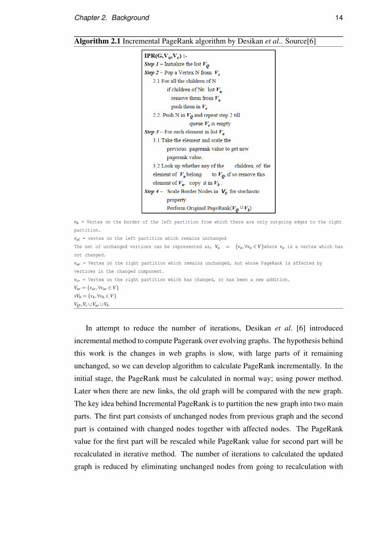
Algorithm 2.1 Incremental PageRank algorithm by Desikan et al.. Source[6]
vb = Vertex on the border of the left partition from which there are only outgoing edges to the right
partition.
vul = vertex on the left partition which remains unchanged
The set of unchanged vertices can be represented as, Vu = {vu,∀vu ∈V}where vu is a vertex which has
not changed.
vur = Vertex on the right partition which remains unchanged, but whose PageRank is affected by
vertices in the changed component.
vcr = Vertex on the right partition which has changed, or has been a new addition.
Vur = {vur,∀vur ∈V}vVb = {vb,∀vb ∈V}VQ=Vc ∪Vur ∪Vb
In attempt to reduce the number of iterations, Desikan et al. [6] introduced
incremental method to compute Pagerank over evolving graphs. The hypothesis behind
this work is the changes in web graphs is slow, with large parts of it remaining
unchanged, so we can develop algorithm to calculate PageRank incrementally. In the
initial stage, the PageRank must be calculated in normal way; using power method.
Later when there are new links, the old graph will be compared with the new graph.
The key idea behind Incremental PageRank is to partition the new graph into two main
parts. The first part consists of unchanged nodes from previous graph and the second
part is contained with changed nodes together with affected nodes. The PageRank
value for the first part will be rescaled while PageRank value for second part will be
recalculated in iterative method. The number of iterations to calculated the updated
graph is reduced by eliminating unchanged nodes from going to recalculation with

Chapter 2. Background 15
power method.
Figure 2.6: Before graph
Figure 2.7: After graph
Figure 2.8: Tagging the graph
Chapter 2. Background 16
As a working example we will start from Figure2.6 where we have 8 nodes. Then
after some times, the graph changed as in Figure 2.7 where we added node 9 and 10
and delete node 8. In Incremental PageRank we will tag the node as in Figure 2.8
before we partition it. We will start from new and deleted node and find all descendant
of it using Breadth-First Search algorithm. Node 6 and 7 are categorised as changed
node because node 6 added new inlink while node 7 lost an inlink. We also will find
all descendant for these two nodes. Node 5 and 4 are unchanged node but it will be
recalculated because their PageRank value is contributed by changed nodes, node 6 and
7. Node 3 will go to recalculation stage but will not be recalculated. Node 3 needed
in recalculation stage because node 3 contributed to PageRank value for node 5. Node
1 and 2 wil just be scaled and will not go to iterative recalculation stage because they
are unchanged and not descendant of changed node.
Incremental PageRank was experimented by Desikan et al. with small dataset
which is just a departmental university website that only need at most 12 iterations
if the PageRank vector is calculated in naïve way. The result of experiment shows
that if the changes between old graph and new graph is less than 5% the number of
iterations needed to recalculate is about 30% - 50% less than naïve way. However, if
the changes is more than 50%, it only can save 2 iterations out of 12 iterations. The
good thing about this method is the PageRank value is exactly the same compared to
naïve update. On the other hand, the problem with this method is if there is a new node
pointing to a node that large number of descendants. It will create a ripple effect and
will bring all descendants to iterative stage. Let say the nodes have a million connected
to it and later on it just add one new node. The addition will not affect that much on
current PageRank but the effort taken to recalculate the PageRank is so big.
Lin and Schatz managed to reduce works per iteration by 69% using Hadoop frame-
work and implemented design pattern called “Schimmy” for calculating PageRank on
Carnegie Mellon University ClueWeb09 collection of web graph with 1.4 billion edges
in [13]. The size of collection is coincidentally similar to Twitter data by Kwak et al.
in [11]. Schimmy is a combination of the authors’ name, Schatz and Jimmy. The idea
behind this Schimmy design pattern is message passing. The message passing design
pattern is claimed to address issue in existing best practices for MapReduce graph
algorithms that have significant shortcomings which limit performance, especially
with respect to partitioning, serializing, and distributing the graph. Typically, such
algorithms iterate some number of times, using graph state from the previous iteration
as input to the next iteration, until some stopping criterion is met.
Chapter 2. Background 17
Lin and Schatz explained that in the basic PageRank algorithm implementation
in Hadoop MapReduce framework, there are two separate dataflows from mappers
to reducers. First, messages passed from source to destination vertices and then
the graph structure itself. By emitting each vertex’s structure in the mapper, the
appropriate reducer receives messages destined for that vertex along with its structure.
This allows the reducer to perform a computation and to update the graph structure,
which is written to disk for the next iteration. Since the algorithms such as graph
partitioning and breadth first search are iterative and require multiple MapReduce jobs,
it is highly inefficient to shuffle the graph structure between the map and reduce phases.
Frequently, the output in reducers much larger than in mappers because it includes
graph structure with metadata and other state information.
The main idea behind the schimmy design pattern is the parallel merge join.
Suppose the input key-value pairs representing the graph structure were partitioned
into n files (i.e., parts), such that G = G1∪G2∪ ...∪Gn, and within each file, vertices
are sorted by vertex id. The same partition function will be used as the partitioner
in MapReduce graph algorithm, and the number of reducers is equal to the number of
input files (i.e., parts). This guarantees that the intermediate keys (vertex ids) processed
by reducer R1 are exactly the same as the vertex ids in G1; the same for R2 and G2,R3
and G3, and so on up to Rn and Gn. Since the MapReduce execution framework
guarantees that intermediate keys are processed in sorted order, the corresponding Rn
and Gn parts are also sorted in exactly the same manner. The intermediate keys in
Rn represent messages passed to each vertex, and the Gn key-value pairs comprise the
graph structure. Therefore, a parallel merge join between R and G suffices to unite
the result of computations based on messages passed to a vertex and the vertex’s
structure, thus enabling the algorithm to update the vertex’s internal state. They
managed to eliminate the need to shuffleG across the network. With the MapReduce
implementation of PageRank using the schimmy design pattern, there is no need to
emit the graph structure in the map phase of processing. Thus, we can reduce work by
per iteration for calculating PageRank.
Previously, studies involving evolving graphs rely heavily on small dataset and
sometimes synthetic dataset due to lack of access to big public dataset. Now,
researchers especially social media analysts can crawl Twitter data via Twitter API
and do research on evolving graphs. Kwak et al. managed to crawl the entire Twitter
user profiles as until June 31st, 2009 and did the first quantitative study on the entire
Twittersphere and information diffusion on it [11]. Kwak et al. compared three ranking
Chapter 2. Background 18
methods to rank Twitter users. First they rank by number of follower, then PageRank
and followed by retweet.
The results shows that there is big difference in ranking of Twitter user when
ranking results are compared. In other words, if the user has many followers, it will be
reflected in PageRank value, but if the user has high number of follower and PageRank
value it will not be reflected in their tweets will be retweeted by those who subscribed
to their tweets. They also found out that following is not so mutual among Twitter
users as the result shows only 29% of Twitter user followed each other. This is because
Twitter used “I follow you” concept rather than “We are friend” like in Facebook and
MySpace. In its follower-following topology analysis they have found a non-power-
law follower distribution, a short effective diameter, and low reciprocity, which all
mark a deviation from known characteristics of human social networks [14].
In [11], other than ranking, the authors also analyzed the tweets of top trending
topics and reported on the temporal behavior of trending topics and user participation.
They classify the trending topics based on the active period and the tweets and show
that the majority (over 85%) of topics are headline or persistent news in nature. A
closer look at retweets reveals that any retweeted tweet is to reach an average of 1, 000
users no matter what the number of followers is of the original tweet. Once retweeted,
a tweet gets retweeted almost instantly on the 2nd, 3rd, and 4th hops away from the
source, signifying fast diffusion of information after the 1st retweet.
Kwak et al. did not mention how they processed the 1.47 billion following relations
in [11] nor how they did the PageRank calculation. Information like how many
iterations until the PageRank vector converged and the epsilon threshold are also not
available for us to compare. We decided to compare the top 10 Twitter users in their
report with our result as a cross-checking to evaluate our method since we are going
to use the data made available by them. The result might be different because of
the choice of epsilon threshold parameter to terminate the iteration in power method.
In addition, the result will be different if the method to calculate PageRank is either
approximation or exact value method.

Chapter 3
Incremental+ PageRank
3.1 Approach Proposal
Desikan et al. incremental method [6] can be implemented with Hadoop environment
with a challenge. The challenge is to find all the nodes affected if addition or deletion
of nodes occured. Again we will use iterative approach such breadth-first search to find
all the descendants of changed nodes. This is the overhead of the method in exchange
of less iteration in power method.
We proposed a solution that can maximised the benefit of incremental method. All
Twitter users with a large number of follower will not be recalculated in iterative stage
even though there is new follower following them except if the changes is more than
the threshold that we have set.
For example, we will set the threshold to 1% and if user A has 10,000 and in later
stage user A has 10,050 or 9,550 followers, we wil not recalculate PageRank for this
particular Twitter user. We will only recalculate if and only if the changes is at least to
11,000 or 9,000. We also will not bring all the descendants to the recalculation stage.
This additional step will help us to reduce the number of iterations.
For naming convention, Desikan et al. original incremental method [6] will be just
called Incremental method and our incremental method with threshold will be called
Incremental+ ( pronounce incremental plus).
19

Chapter 3. Incremental+ PageRank 20
3.2 Hypotheses
3.2.1 First Hypothesis
H10 : Mean time per iteration to calculate PageRank is same for every method.
H1a : At least there is one method is different in mean time per iteration to calculate
PageRank based on methods.
3.2.2 Second Hypothesis
H20 : At least one of the methods will not produce the same ranking result for Twitter
user.
H2a : All the methods to calculate PageRank will produce the same ranking result for
Twitter user.

Chapter 4
Experimental Framework
This chapter outlines various experimental settings. The conceptual designs of the
experiments come from a number of decisions which are also discussed. We firstly
introduce the main dataset and explain experiment procedure in a calculating PageRank
with naïve, Desikan et al. Incremental PageRank and our version of incrementally
PageRank with treshold methods. Finally we discussed evaluation methods.
4.1 Hadoop Cluster
We are so lucky to to process 1.47 billion following relation data and run our
experiments on a Hadoop Cluster . This Hadoop Cluster is belong to Statistical
Machine Translation Group of University of Edinburgh. This cluster has 8 working
datanodes and 48TB of storage with 50GB RAM per node. This cluster is installed
with Hadoop version 0.19.2-dev. The number of Mapper is 250 while the number of
Reducer is 72. We will run and test our code on local machine before run it on Hadoop
Cluster.
4.2 Dataset
Twitter offers an Application Programming Interface (API) that is easy to crawl and
collect data. Again, we are so lucky to have Twitter user profiles already available for
processing. This data was crawled by social media analyst research group from Korean
Advanced Institute of Technology KAIST). They published a paper on Twitter tweets
stream analysis and Twitter user topological relation graph and ranking in [11]. This
data is available for public download at http://an.kaist.ac.kr/traces/WWW2010.html.
21

Chapter 4. Experimental Framework 22
The file is in the following format: USER \t FOLLOWER \n. (\t is tab and \n
is newline). USER and FOLLOWER are represented by numeric ID (integer) and
same as numeric IDs Twitter managed. So we can access a profile of user 123 via
http://api.twitter.com/1/users/show.xml?user_id=123.
Example of data:1 2
1 3
2 4Based on example above, 1 is following 2 and 3 while 4 is followed by 2. In
order to collect user profiles, Kwak et al. began with Perez Hilton who has over
one million followers and crawled breadth-first along the direction of followers and
followings. Twitter rate limits id 20,000 requests per hour per whitelisted IP. Using 20
machines with different IPs and self-regulating collection rate at 10,000 requests per
hour, they collected user profiles from July 6th to July 31st, 2009. Overall there are
147 compressed files with cumulated size of 8GB.
4.3 Data Preprocessing
There are 1.47 billion of following relations and sorted in ascending or by follower id.
In order to emulate incremental environment we have to partition the data into three
parts. The data does not consists of history of when the relation is created. If we have
we can easily divided the data according to date that we will set date as threshold.
Unfortunately we do not have that information, therefore, we will randomly shuffle the
position of sorted data before we group into parts. First part is unchanged relations,
then the second part will consists of additional relations followed by third part which
contains deleted relations. Randomness is very important to make sure it emulates real
world application where Twitter user will follow based on other follower or followee
list and will unfollow whomever they feel to unfollow.
There is no official report about the user retention and how fast is Twitter user
growing. There is an unofficial online report1 stating that the user retention is around
40% but this is just approximation and not very reliable to be ground foundation for our
decision. We decided to use classical Pareto Distribution2 or also known as 80-20 rule.
The data will be divided to 80% unchanged and 20% changed. The 20% part is consists
1http://blog.nielsen.com/nielsenwire/online_mobile/twitter-quitters-post-roadblock-to-long-term-growth/
2http://en.wikipedia.org/wiki/Pareto_distribution
Chapter 4. Experimental Framework 23
of 15% of new following relations while the remaining 5% is for deleted relation. We
will have two different final experiment datasets for the purpose of repetition and avoid
bias and skewed result. It is also important to avoid overfitting.
4.4 PageRank variable setting
Rk+1(u) =1−d
N+d ∑
v∈Bu
Rk(v)Nv
(4.1)
Ro(v) =
1 ,v ∈ Bu 6= 0
1−dN ,v ∈ Bu = 0
(4.2)
We will use PageRank formula based on Random Surfer Model with power method
as in Figure4.1. We will set damping factor, d = 0.85 and iteration termination
threshold ε = 0.0001. This setting is based on normal setting by other experiments
like in [15, 8][15, 8]. At initial stage or iteration k = 0, we will set initial PageRank
value, R0(v) = 1 and R0(v) = 1N if the node does not have any inlinks as in Equation
4.2. The reason for setting R0(v) = 1 for any other nodes with inlinks is on assumption
that the Twitter user has at least one follower. We do not set nodes with inlinks with1N as suggested in [12] because our N is so big as in million and the value will too
small. The main reason for setting R0(v) =1−dN for node without any inlinks is to help
our PageRank calculation to meet the convergence quicker because the value will not
change after first iteration.
4.5 Experiment Procedures
4.5.1 The Before Graph
Calculate Σ| Rt – Rt-‐1 |
Calculate PageRank
Ini5alize
If Σ| Rt – Rt-‐1 | > ε
Start
End
YES
NO
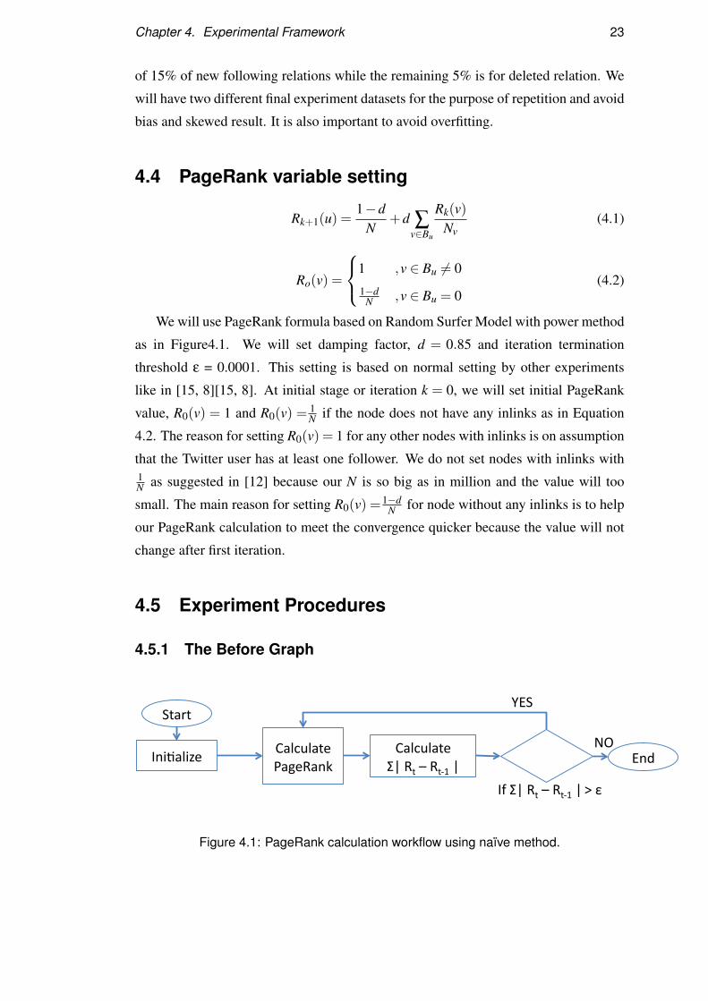
Figure 4.1: PageRank calculation workflow using naïve method.

Chapter 4. Experimental Framework 24
Algorithm 4.1 MapReduce algorithm for naïve method.1. Initialize
1.1 Map
1.1.1 Input : k: follower \t v: followee
1.1.2 Output:
k: follower v: followee
k: followee v: follower
1.2 Reduce
1.2.1 Output: k: follower \t v: old PageRank | new PageRank | outlinks
2. Calculate PageRank
2.1 Map
2.1.1 Input: k: follower \t v: old PageRank | new PageRank | outlinks
2.1.2 Output:
k: follower v: old PageRank | outlinks
For every outlinks:
k: followee v: new PageRank=(0.15/N) + (0.85*old PageRank)
2.2 Reduce
2.2.1 Output: k: follower \t v: old PageRank | new PageRank | outlinks
3. Calculate Total Residual
3.1 Map
3.1.1 Input: k: follower \t v: old PageRank | new PageRank | outlinks
3.1.2 Output: k: difference v: new PageRank - old PageRank
3.2 Reduce
3.2.1 Output: k: total residual \t v: sum of difference
Repeat 2 and 3 until total residual < ε
Note : k is key, v is value
First, we will calculate PageRank value for the graph at time before any changes
happen, we call it at time,Gt . We will use Hadoop Map Reduce to compute the
PageRank Value. There will be three MapReduce jobs as illustrated in Figure 4.1.
In the first job we will read the input in edge list format or also known as following list
into adjacency list that will list follower and outlinks or also known as followee list.
We also initialise the PageRank value as in Equation 4.2. The output from reducers in
initialisation stage will be input in the next job to calculate PageRank value. It is also
worth to note that we should use BigDecimal type when we calculate PageRank value
instead of float or double value type, because there is accuracy issue in Java float and
double type especially in division operation. We just use BigDecimal as for calculation
Chapter 4. Experimental Framework 25
but we still output it as Text to next job. In the next job we calculate the absolute value
of difference between previous PageRank and current PageRank in the map phase and
in the reduce phase we will sum the value. In the next step we use unix shell command
to check whether the sum is greater or smaller than ε value. If the sum value is less
than ε, then we will stop the iteration otherwise we keep calculate the PageRank value
until it reach termination criterion. It is a good practice to delete output from previous
iteration so that our server will not get full by temporary results. Another good practice
is to use Hadoop MapReduce -mv (move) shell command instead of -cp (copy) before
take one ouput from previous job as input in another job.
4.5.2 The After Graph
4.5.2.1 Baseline
In the next step we calculate the PageRank value for the graph at after changes happen,
we call it at Gt+1. As a baseline for comparison with other methods, we will calculate
the PageRank value same way we calculate the PageRank value for the graph at Gt .
We will record the number of iterations and time to complete.
4.5.2.2 Incremental PageRank
Calculate Σ| Rt – Rt-‐1 |
Calculate PageRank
If Σ| Rt – Rt-‐1 | > ε
Start End
YES
NO
Preprocess Gt
Preprocess Gt+1
Tagging DifferenGate
ParGGon
Merge SGll gray?
YES
NO
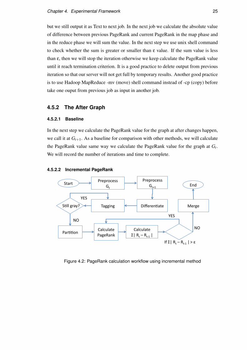
Figure 4.2: PageRank calculation workflow using incremental method
Chapter 4. Experimental Framework 26
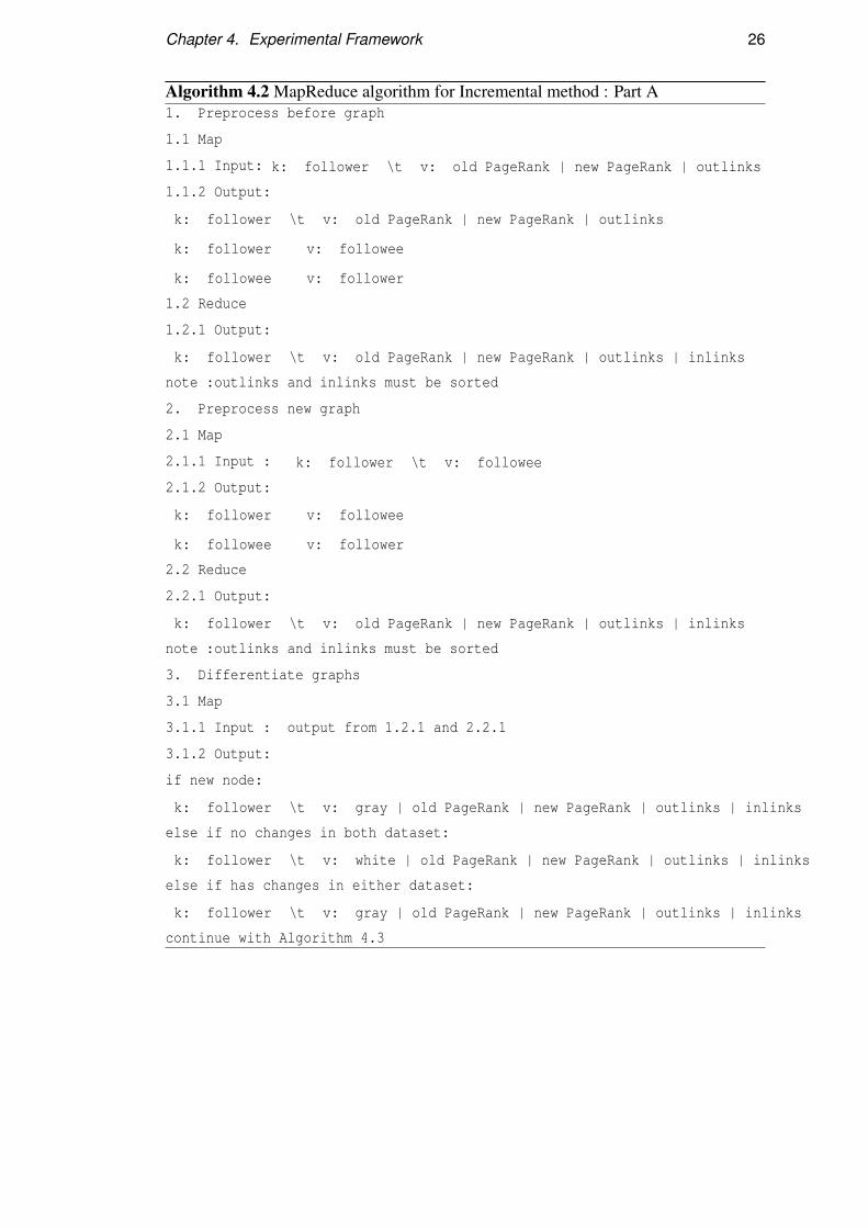
Algorithm 4.2 MapReduce algorithm for Incremental method : Part A1. Preprocess before graph
1.1 Map
1.1.1 Input: k: follower \t v: old PageRank | new PageRank | outlinks
1.1.2 Output:
k: follower \t v: old PageRank | new PageRank | outlinks
k: follower v: followee
k: followee v: follower
1.2 Reduce
1.2.1 Output:
k: follower \t v: old PageRank | new PageRank | outlinks | inlinks
note :outlinks and inlinks must be sorted
2. Preprocess new graph
2.1 Map
2.1.1 Input : k: follower \t v: followee
2.1.2 Output:
k: follower v: followee
k: followee v: follower
2.2 Reduce
2.2.1 Output:
k: follower \t v: old PageRank | new PageRank | outlinks | inlinks
note :outlinks and inlinks must be sorted
3. Differentiate graphs
3.1 Map
3.1.1 Input : output from 1.2.1 and 2.2.1
3.1.2 Output:
if new node:
k: follower \t v: gray | old PageRank | new PageRank | outlinks | inlinks
else if no changes in both dataset:
k: follower \t v: white | old PageRank | new PageRank | outlinks | inlinks
else if has changes in either dataset:
k: follower \t v: gray | old PageRank | new PageRank | outlinks | inlinks
continue with Algorithm 4.3
Chapter 4. Experimental Framework 27
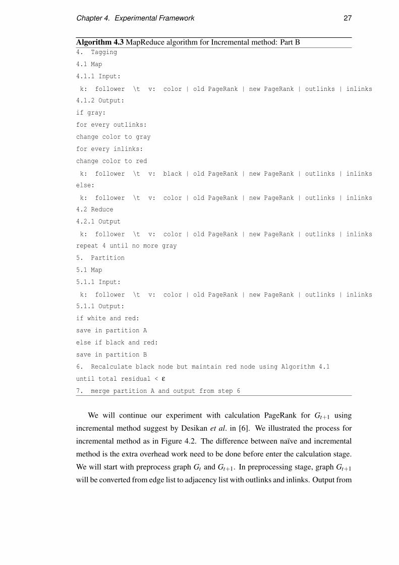
Algorithm 4.3 MapReduce algorithm for Incremental method: Part B4. Tagging
4.1 Map
4.1.1 Input:
k: follower \t v: color | old PageRank | new PageRank | outlinks | inlinks
4.1.2 Output:
if gray:
for every outlinks:
change color to gray
for every inlinks:
change color to red
k: follower \t v: black | old PageRank | new PageRank | outlinks | inlinks
else:
k: follower \t v: color | old PageRank | new PageRank | outlinks | inlinks
4.2 Reduce
4.2.1 Output
k: follower \t v: color | old PageRank | new PageRank | outlinks | inlinks
repeat 4 until no more gray
5. Partition
5.1 Map
5.1.1 Input:
k: follower \t v: color | old PageRank | new PageRank | outlinks | inlinks
5.1.1 Output:
if white and red:
save in partition A
else if black and red:
save in partition B
6. Recalculate black node but maintain red node using Algorithm 4.1
until total residual < ε
7. merge partition A and output from step 6
We will continue our experiment with calculation PageRank for Gt+1 using
incremental method suggest by Desikan et al. in [6]. We illustrated the process for
incremental method as in Figure 4.2. The difference between naïve and incremental
method is the extra overhead work need to be done before enter the calculation stage.
We will start with preprocess graph Gt and Gt+1. In preprocessing stage, graph Gt+1
will be converted from edge list to adjacency list with outlinks and inlinks. Output from

Chapter 4. Experimental Framework 28
converged PageRank vector for Gt also will be converted to adjacency list of outlinks
and inlinks. It is worth to note that in Hadoop MapReduce, only the key will be sorted
but the values are not. Sometimes output from MapReduce job will be 1\t2,3,4 and
sometimes it will output as 1\t3,4,2 (\t stands for tab). Therefore if we are going to do
comparison the system will say that this two list are not the same but in fact they are
the same list. So we have to make sure the order of outlinks and inlinks are the same.
Next, we will differentiate this two graphs. In Hadoop MapReduce we can
compare two different datasets by setting the input parameter for MapReduce job as
CompositeInputFormat class and set join expression to outer join. The reason we
use outer join is to detect any missing or new record compared to the graph Gt . In
differentiating stage, we will check if the record is not exist in before graph, we will
tag it as new record and set the initial PageRank value as in Equation 4.2. If the record
is appear in both graph and the number of outlinks and inlinks are same, we will output
as it is, but if there is different in the number of outlinks or inlinks we will output to
next stage with previous PageRank value and latest outlinks and inlinks list. By doing
this, the calculation we be faster to converge as we use previous PageRank value to
calculate. All the previous PageRank value will be rescaled (previous PageRank value
multiply the number of nodes in previous Gt and then divide by the number of nodes
in Gt+1). All nodes will be tag with either gray color or white. Color gray is for new
nodes and changed nodes while white is for unchanged nodes.
After that we will continue to the tagging stage. In tagging stage we will start
with all nodes tagged with gray color will be processed and changed to black color
and subsequently changed the color of nodes in its outlinks to gray color too and the
nodes in its inlinks will be changed to red color to remark as border nodes. In the
next iteration it will do the same until there is no more gray color left. In Hadoop
MapReduce we keep track the number of gray nodes with Custom Counter class. All
white nodes will be remained as it is.
We will continue to partition all the white and red nodes as one output and we do
not have to do recalculate this partition as we already rescaled the PageRank value in
preprocessing stage. All the black nodes and red nodes will go to recalculation stage.
The reason we bring the red nodes is because this nodes are contributing to black nodes
PageRank value, but we do not recalculate the value of red nodes themselves. After
convergence, we will merge the output from the partitioned output and the output from
this stage as final PageRank vector output.

Chapter 4. Experimental Framework 29
4.5.2.3 Incremental+ PageRank
Calculate Σ| Rt – Rt-‐1 |
Calculate PageRank
If Σ| Rt – Rt-‐1 | > ε
Start End
YES
NO
Preprocess Gt
Preprocess Gt+1
Tagging DifferenGate
Verify
Merge
ParGGon
SGll gray?
YES
NO
Figure 4.3: PageRank calculation workflow using incrementa+l method
Algorithm 4.4 MapReduce algorithm for Incremental+ method1. Follow all step in Algorithm 4.2 and continue with step 4 in
Algorithm 4.3
2. Verify
2.1 Map
2.1.1 Input : output from 1.2.1 from Algorithm 4.2 and 4.2.1 from
Algorithm 4.3
2.1.2 Output:
if descendant of changed node && black && no new outlink && number of new
inlinks less than threshold:
change to white and save to partition A
else:
remain color and partition accordingly
3. Recalculate black node but maintain red node using Algorithm 4.1
until total residual < ε
4. merge partition A and output from step 3
The next step is to run experiment using our version of incremental PageRank
update with threshold method also known as Incremental+ method. All the step is same
with Desikan et al. method but we add extra stage. After tagging stage, we will find

Chapter 4. Experimental Framework 30
all nodes tagged as black color and the number of outlinks is the same with previous
graph. The reason it must be nodes with same number of outlinks from previous state is
it will not point to any new node that need it as border node for recalculation purpose.
Then we check if the number of inlinks is changed either less or more compared to
previous graph. If the new addition is bigger than threshold percentage, let say 10%
of the number of inlinks in previous graph, we will remained the color tag as black
and recalculate the PageRank value for the node. Otherwise, we change change the
color to white and do not need to recalculate the PageRank for the particular node.
The reason we do not incorporate this in tagging stage is because tagging stage is an
iterative mode. By separating the process we will just run it once, thus we can save the
computation time. As we just approximate the verified node with previous and scaled
PageRank value, we will calculate the mean squared error compared to the actual value
of PageRank calculated using naïve method.
4.6 Evaluation Methods
We will discuss about the methods we used to evaluate our method for calculating
PageRank. We will look into two perspectives. First, how efficient is our method
based on time cost and workload. Then we will look into how effective is our method.
We will use Root Mean Square Error (RMSE) and Kendall’s Tau coefficient to measure
the effectiveness of our method.
4.6.1 Efficiency
We need to measure how our method can save time and reduce workload when
calculate PageRank value compared to other methods.
4.6.1.1 Time cost
We have three methods to compare so we used ANalysis Of VAriance between groups
(ANOVA) for significant test instead of student-T Test to compare the means of time
taken to calculate PageRank per iteration. We will combine the time to finished
the job in calculating PageRank and job to calculate the sum of residual at each of
every iteration. Sum of residual is the difference between previous rank and current
rank. Our first hypothesis null, H10 : all the method took the same amount of time
to calculate PageRank per iteration. We will used 5% significance level, so at 5%

Chapter 4. Experimental Framework 31
significant level if F-ratio > 3.68, we can reject H10 and can say that the time taken to
calculate PageRank per iteration is not the same. Then, we will do post-hoc analysis
to find which method is the best.
We also used descriptive statistics to compare the three methods. The information
that we compared are the time taken to finished the whole process, the number of
iterations and used Faster metrics as used by Desikan et al. in [6]. The method with the
least time taken to finish the whole process of calculating PageRank is considered the
best. On the other hand, the method with largest value of metrics Faster is considered
the best. Desikan et al. defined the metrics Faster to compare how fast if compared to
base method as follows.
Number of Times Faster = Number of Iterations for Based Method / (1 + (fraction
of changed portion) * (Number of Iterations for Improved Method ))
4.6.1.2 Workload
Next, we used information such as how many input going for recalculation and from
this information we can derive how many input we can save from recalculation when
compared with another method. This is as suggested by Langville and Meyer in [12],
in order to measure how many works we reduce per iteration. The best method will
have the highest percentage of input prevented to go to recalculation stage. We also
will pair with extra overhead cost in order to get the savings, as a penalty measure.
4.6.2 Effectiveness
We also need to measure how accurate our method compared to other methods. The
most common measurement for accuracy is Root Mean Square Error while Kendal’s
Tau coefficient is best for measuring which ranker is the best when compared.
4.6.2.1 Root Mean Square Error (RMSE)
Root Mean Square Error (RMSE) is a common statistical tool to measure the
differences between values predicted by a model or an estimator and the values actually
observed from the thing being modeled or estimated. In our case we will compare the
PageRank value computed by Incremental+ with PageRank value computed with naïve
method which is the exact or true value. We have to calculate Root Mean Square
Error (RMSE) for our version of incremental PageRank because we approximated
the PageRank value for the nodes that has no changes in the number of outlinks but

Chapter 4. Experimental Framework 32
has changes in the number of inlinks, either addition or deletion that is less than
the threshold that we set. In our experiments we set our threshold as 10%. If the
value is RMSE small or near zero it means we can conclude that our model is a
good approximator and effective ranker. The formula for root mean square error is
as follows.
RMSE(θ1,θ2) =
√√√√ n∑
i=1(x1,i− x2,i)2
n(4.3)
4.6.2.2 Kendall’s Tau coefficient
Kendall rank correlation coefficient, commonly referred to as Kendall’s tau (τ)
coefficient, is a statistic used to measure the association between two measured
quantities. There are few variations of Kendall’s Tau formula. We used the simplest
formula of Kendall’s tau coefficient as follows.
K(τ) =P−QP+Q
(4.4)
P = Number of correctly-ordered pairs
Q = Number of incorrectly ordered pairs
Our second null hypothesis regarding efficiency in ranking are:
H20 :The ranking order of whole Twitter user of our version of incremental
PageRank is not the same as ranking order by Desikan et al. Incremental PagRank
method.
If our Kendall’s tau value is equal to 1 for comparison among rankers, then we can
reject second null hypothesis and claim that our method produce the same ranking as
other methods.
Chapter 5
Experimental Evaluations
In this chapter we present and discuss experimental results based on experimental
framework we discussed in previous chapter. Descriptive analysis along two di-
mensions; efficiency and effectiveness is discussed in the first part. On the second
part we present the hypotheses testing results as the ground judgment to evaluate
our Incremental+ PageRank method. For naming convention, Desikan et al. original
incremental method [6] will be just called Incremental method and our incremental
method with threshold will be called Incremental+ ( pronounce incremental plus).
5.1 Efficiency
5.1.1 Time cost
-‐6
-‐4
-‐2
0
2
4
6
8
10
9 19 29 39 49 59 69 79 89 99 109 119 129 139
naïve incremental incremental+
log residual vs itera>on
Log residu
al
itera>on
Figure 5.1: Rates of convergence
33

Chapter 5. Experimental Evaluations 34
In dimension of efficiency, we focused our evaluation on the performance of our
method based on time cost and task workload. For time cost evaluation, method that
took less time to finish the process to produce output is considered as a better method.
In addition, the less workload we put on desired task also will produce faster result.
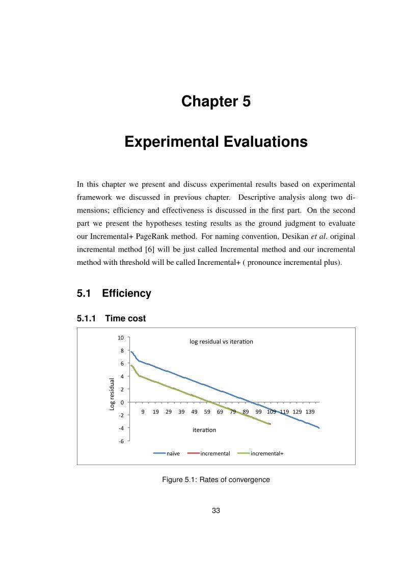
For every method we used to calculate PageRank vector, we plotted the log value
of residual for each iteration and present it in Table 5.1. Residual is the total difference
of current PageRank from previous iteration. We use log instead of the real value of
residual for better visual representation and data analysis. It help us to see how each
method reach convergence and the rate of convergence. All methods have faster rate of
convergence in first eight iterations and after that it become slower in gradual manner.
We can see that naïve method took longer time to converge compared to Incremental
and Incremental+ method. Another observation can be made is, if we look closely,
Increment+ log residual value is on top incremental method. It shows that the values is
very close and we can see only a little red line visible representing Incremental method
log residual value. This is because Incremental+ has only less one iteration compared
to Incremental method.
Method Number of iteration Iteration
Saved
Faster
naïve 147 - -
incremental 109 25.85% 6.45
incremental+ 108 26.53% 6.50
Table 5.1: Percentage of iteration saved
We continued our evaluation on how efficient is our method compared to others by
looking on how many iteration saved for calculating the PageRank vector as in Table
5.1. We save 26.53% by ommiting the new inlinks that is just too small to contribute
to PageRank value for Twitter user that has large number of follower. However, the
difference is just 0.68% compared to Incremental method or in other words, we only
have one less iteration. The faster column in Table 5.1 is based on Desikan et al.
metrics to evaluate how fast is the method compared to naïve method. The formula
is discussed as in Equation in previous chapter. This formula is not just comparing
number of iteration but also incorporated the percentage of changes portion in the
graph. This extra effort is to approximate measure to compare the computational cost
versus the naïve method.

Chapter 5. Experimental Evaluations 35
Method Time to complete (seconds) Overhead cost (seconds)
naïve 162,846 1,142
incremental 114,040 8,626
incremental+ 116,904 10,562
Table 5.2: Overhead cost for time to complete
Even though there is visible difference in term of reduced number of iteration
in power method, we also have to measure how much is overhead cost to get less
iteration and less time to complete the task. We present the overhead cost as in Table
5.2. Overhead for naïve method is just to convert from edge list to adjacency list and
intialize the PageRank value and it took about 45 hours to calculate PageRank vector.
For Incremental method it took 32 hours to complete the task and need to 2.4 hours to
differentiate the graphs and partition it before into recalculation stage. Incremental+
need extra 30 minutes compared to Incremental method for verifying and preventing
some affected nodes from being into recalculation stage.
Number of
iterations
for tagging
Time taken
for tagging
(seconds)
Changed nodes Affected nodes
10 5,583 221,543 41,567,014
Table 5.3: Ripple effect in incremental method
Next, we look into which component in both incremental and incremental+ method
that cost a lot of time based on the overhead cost. Based on result in Table 5.3, more
than 50% of overhead cost is contributed by tagging operation, where we find all
affected nodes which are the descendants of changed nodes. The tagging stage is based
on breadth-first seach algorithm and this algorithm requires iterative implementation.
Tagging stage will cause ripple effect or viral effect as we can see that only 22
thousand changed nodes but they are affecting 42 million descendants nodes and it
took 10 iterations to tag all affected descendants. The most important observation is
for iteration number 7 to 10, it only affecting one node for each iteration. It is such a
waste of time and computing resources just to find and tag a single affected node. This
is the main danger of incremental method that we should aware of. Maybe we can
use the same idea with incremental+ method which is using threshold to improve this

Chapter 5. Experimental Evaluations 36
matter in future by stopping the tagging stage when it reach less than certain number
of nodes and these nodes also has less than certain number of descendants.
naïve incremental incremental+
Sampel size 147 109 108
Mean 778.67 680.57 683.10
Std. Deviation 78.060 113.970 25.528
Std. Error 6.438 10.916 2.456
Confidence
Interval for
Mean
Lower Bound 765.95 658.93 678.23
Upper Bound 791.40 702.21 687.97
Minimum 615 537 640
Maximum 947 1080 770
Table 5.4: Descriptive statistics of time per iteration to calculate PageRank
We further our investigation on performance evaluation by looking into time per
iteration to calculate PageRank. PageRank calculation is based on power method and
involve many iterations. We would like to know which method will require less time to
calculate PageRank vector. The early analysis is by doing descriptive statistics on time
per iteration as shown in Table 5.4. Sample size is limited to number of iterations for
each method. In this stage, we can judge the performance the performance by looking
at the average value or also known as mean value, but we have to do ANOVA if we
want to compare the means in more meaningful and statistically significant.

Chapter 5. Experimental Evaluations 37
Figure 5.2: Box plot for time per iteration to calculate PageRank
We compared dataset side by side using box plot as in Figure5.2. Box plot is
very useful for us to look for early indication about the data symmetry and skewness.
This information is very important regarding using ANOVA as method to compare
means. We also can spot outliers in the Incremental and Incremental+ time per iteration
dataset. Incremental+ has the smallest variance, followed by naïve and Incremental
method.
5.1.2 Workload
Method Number of inputs into
recalculation stage
Workload Saved
naïve 41,589,858 -
incremental 41,567,014 0.05%
incremental+ 41,500,793 0.21%
Table 5.5: Dataset 1 : Number of input into recalculation stage
In this sub section, we explored the result that contribute to main idea of Incremental+
method. The main idea behind Incremental+ method is to reduce the number of
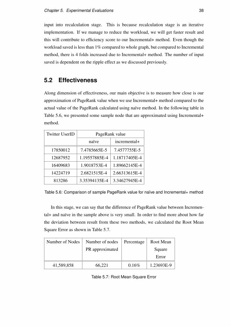
Chapter 5. Experimental Evaluations 38
input into recalculation stage. This is because recalculation stage is an iterative
implementation. If we manage to reduce the workload, we will get faster result and
this will contribute to efficiency score to our Incremental+ method. Even though the
workload saved is less than 1% compared to whole graph, but compared to Incremental
method, there is 4 folds increased due to Incremental+ method. The number of input
saved is dependent on the ripple effect as we discussed previously.
5.2 Effectiveness
Along dimension of effectiveness, our main objective is to measure how close is our
approximation of PageRank value when we use Incremental+ method compared to the
actual value of the PageRank calculated using naïve method. In the following table in
Table 5.6, we presented some sample node that are approximated using Incremental+
method.
Twitter UserID PageRank value
naïve incremental+
17850012 7.4785665E-5 7.4577755E-5
12687952 1.19557885E-4 1.18717405E-4
16409683 1.9018753E-4 1.89662145E-4
14224719 2.6821515E-4 2.66313615E-4
813286 3.35394135E-4 3.34627945E-4
Table 5.6: Comparison of sample PageRank value for naïve and Incremental+ method
In this stage, we can say that the difference of PageRank value between Incremen-
tal+ and naïve in the sample above is very small. In order to find more about how far
the deviation between result from these two methods, we calculated the Root Mean
Square Error as shown in Table 5.7.
Number of Nodes Number of nodes
PR approximated
Percentage Root Mean
Square
Error
41,589,858 66,221 0.16% 1.23693E-9
Table 5.7: Root Mean Square Error
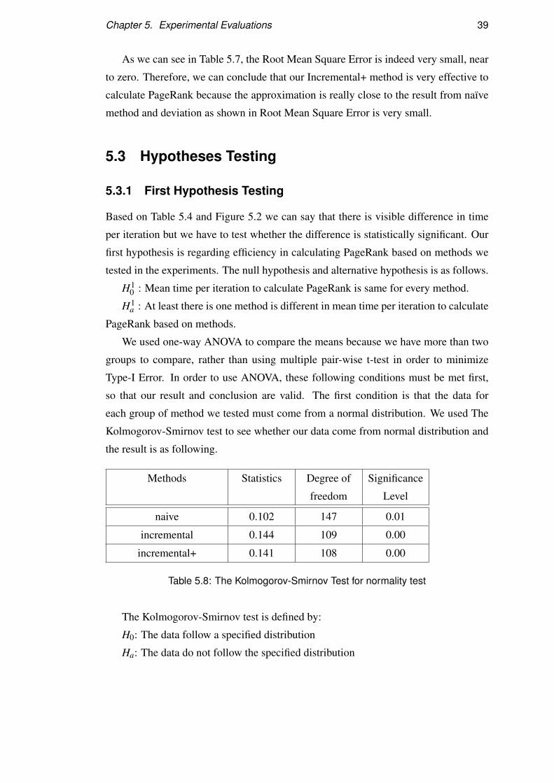
Chapter 5. Experimental Evaluations 39
As we can see in Table 5.7, the Root Mean Square Error is indeed very small, near
to zero. Therefore, we can conclude that our Incremental+ method is very effective to
calculate PageRank because the approximation is really close to the result from naïve
method and deviation as shown in Root Mean Square Error is very small.
5.3 Hypotheses Testing
5.3.1 First Hypothesis Testing
Based on Table 5.4 and Figure 5.2 we can say that there is visible difference in time
per iteration but we have to test whether the difference is statistically significant. Our
first hypothesis is regarding efficiency in calculating PageRank based on methods we
tested in the experiments. The null hypothesis and alternative hypothesis is as follows.
H10 : Mean time per iteration to calculate PageRank is same for every method.
H1a : At least there is one method is different in mean time per iteration to calculate
PageRank based on methods.
We used one-way ANOVA to compare the means because we have more than two
groups to compare, rather than using multiple pair-wise t-test in order to minimize
Type-I Error. In order to use ANOVA, these following conditions must be met first,
so that our result and conclusion are valid. The first condition is that the data for
each group of method we tested must come from a normal distribution. We used The
Kolmogorov-Smirnov test to see whether our data come from normal distribution and
the result is as following.
Methods Statistics Degree of
freedom
Significance
Level
naive 0.102 147 0.01
incremental 0.144 109 0.00
incremental+ 0.141 108 0.00
Table 5.8: The Kolmogorov-Smirnov Test for normality test
The Kolmogorov-Smirnov test is defined by:
H0: The data follow a specified distribution
Ha: The data do not follow the specified distribution

Chapter 5. Experimental Evaluations 40
According to Kolmogorov-Smirnov test, at 95% confidence level, we can reject
null hypothesis because the statistics value is greater than the critical value. Therefore
the data is does not come from normal distribution. Sometimes, statistic test can be
misleading, so we decided to do more test and use graphical method like Normal Q-Q
plot to look at the normality issue. We plotted Normal Q-Q plot for all methods we
tested in the experiments as follows.
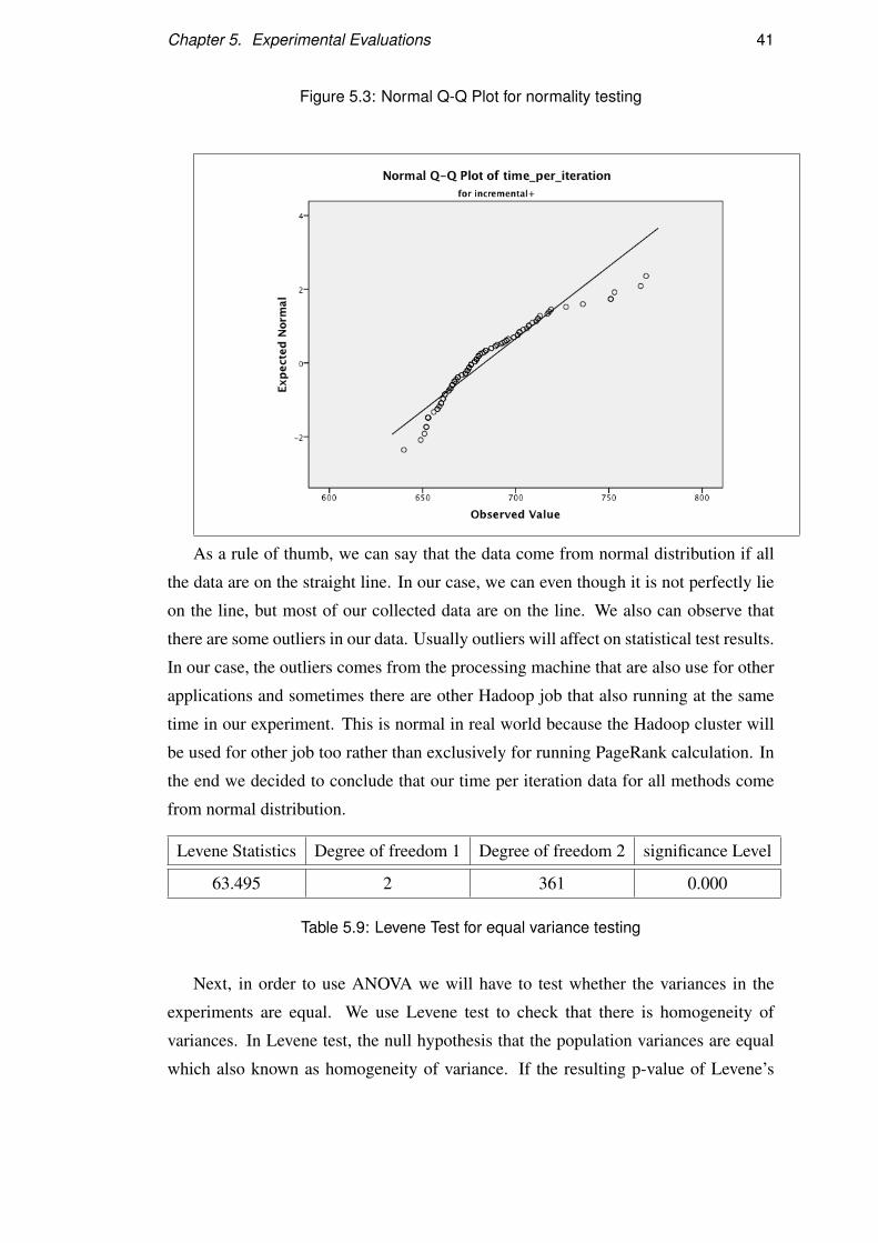
Chapter 5. Experimental Evaluations 41
Figure 5.3: Normal Q-Q Plot for normality testing
As a rule of thumb, we can say that the data come from normal distribution if all
the data are on the straight line. In our case, we can even though it is not perfectly lie
on the line, but most of our collected data are on the line. We also can observe that
there are some outliers in our data. Usually outliers will affect on statistical test results.
In our case, the outliers comes from the processing machine that are also use for other
applications and sometimes there are other Hadoop job that also running at the same
time in our experiment. This is normal in real world because the Hadoop cluster will
be used for other job too rather than exclusively for running PageRank calculation. In
the end we decided to conclude that our time per iteration data for all methods come
from normal distribution.
Levene Statistics Degree of freedom 1 Degree of freedom 2 significance Level
63.495 2 361 0.000
Table 5.9: Levene Test for equal variance testing
Next, in order to use ANOVA we will have to test whether the variances in the
experiments are equal. We use Levene test to check that there is homogeneity of
variances. In Levene test, the null hypothesis that the population variances are equal
which also known as homogeneity of variance. If the resulting p-value of Levene’s
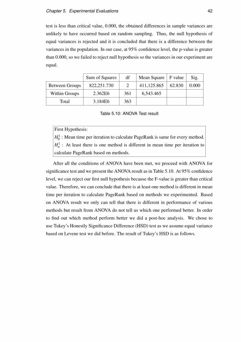
Chapter 5. Experimental Evaluations 42
test is less than critical value, 0.000, the obtained differences in sample variances are
unlikely to have occurred based on random sampling. Thus, the null hypothesis of
equal variances is rejected and it is concluded that there is a difference between the
variances in the population. In our case, at 95% confidence level, the p-value is greater
than 0.000, so we failed to reject null hypothesis so the variances in our experiment are
equal.
Sum of Squares df Mean Square F value Sig.
Between Groups 822,251.730 2 411,125.865 62.830 0.000
Within Groups 2.362E6 361 6,543.465
Total 3.184E6 363
Table 5.10: ANOVA Test result
First Hypothesis:
H10 : Mean time per iteration to calculate PageRank is same for every method.
H1a : At least there is one method is different in mean time per iteration to
calculate PageRank based on methods.
After all the conditions of ANOVA have been met, we proceed with ANOVA for
significance test and we present the ANOVA result as in Table 5.10. At 95% confidence
level, we can reject our first null hypothesis because the F-value is greater than critical
value. Therefore, we can conclude that there is at least one method is different in mean
time per iteration to calculate PageRank based on methods we experimented. Based
on ANOVA result we only can tell that there is different in performance of various
methods but result from ANOVA do not tell us which one performed better. In order
to find out which method perform better we did a post-hoc analysis. We chose to
use Tukey’s Honestly Significance Difference (HSD) test as we assume equal variance
based on Levene test we did before. The result of Tukey’s HSD is as follows.

Chapter 5. Experimental Evaluations 43
I (method) J (method) Mean
Difference
(I-J)
p-value
Std. Error Sig.
naive incremental 98.105* 10.225 0.000
incremental+ 95.572* 10.252 0.000
incremental naive -98.105* 10.225 0.000
incremental+ -2.533 10.983 0.971
incremental+ naive -95.572* 10.252 0.000
incremental 2.533 10.983 0.971
Table 5.11: Tukey’s HSD test result
Based on the result on Table 5.11, at 95% confidence level, we can say that
incremental and incremental+ performed better than naive method in calculating
PageRank because the p-values for these case are greater than critical value. However,
incremental and incremental+ method performance have no significance different
because there is not enough evidence to reject null hypothesis that claim incremental
and incremental+ has the same mean time to calculate PageRank per iteration. Even
though, incremental+ has visible difference as shown in Table 5.5 in saving the inputs
from going to recalculation stage, but apparently the benefit of incremental+ method is
not statistically good enough. Perhaps, in the future we can set the threshold parameter
bigger than 10% so that we can save more inputs from going to recalculation stage.
5.3.2 Second Hypothesis Testing
The main output of PageRank calculation in this dissertation is to rank Twitter user
based on propagation of influential follower. Even though the main formula is same
but the method for calculation may produce different result especially for incremental+
method because we used approximation in calculating PageRank value for certain
affected nodes instead of exact calculation. Our second hypothesis is about the
effectiveness of the ranker based on the ranking result. We stated our second hypothesis
is as follows.
H20 : At least one of the methods will not produce the same ranking result for
Twitter user.

Chapter 5. Experimental Evaluations 44
H2a : All the methods to calculate PageRank will produce the same ranking result
for Twitter user.
Rank Naive Incremental Incremental+ Remark
1 BarackObama BarackObama BarackObama Barack Obama
2 Number10gov Number10gov Number10gov UK Prime Minister
3 WholeFoods WholeFoods WholeFoods Whole Foods Market
4 britneyspears britneyspears britneyspears Britney Spears
5 omnomnome omnomnome omnomnome Nominius N. Nomerson
6 zappos zappos zappos Zappos.com CEO -Tony
7 TheOnion TheOnion TheOnion The Onion
8 BJMendelson BJMendelson BJMendelson Brandon Mendelson
9 threadless threadless threadless Threadless
10 Radioblogger Radioblogger Radioblogger Duane Patterson
Table 5.12: Top 10 Twitter User Ranking
Based on the ranking result of Twitter data in Table 5.12, we can visibly see that
all ranker has the same result but we need to prove it has statistically same result by
applying Kendall’s Tau Test. Kendall’s Tau Test is a non-parametric test to check if the
output from the rankers produce the same ranking result. Kendall’s Tau test is based on
Kendall’s Tau coefficient and can be calculated by using the following formula. K(τ) =P−QP+Q where P is the number of concordant pairs and Q is the number of discordant pairs.
If K(τ) = 1, it means the rankers has the same result, while if K(τ) = −1 the rankers
have opposite ordering of ranking. On the other hand if K(τ) = 0 it means the rankers
have no output with the same ranking at all.
First Ranker Second
Ranker
P Q K(τ)
naive incremental 10 0 1
naive incremental+ 10 0 1
incremental incremental+ 10 0 1
Table 5.13: Kendall’s Tau Test result.
We can reject our second hypothesis null, H20 , if at least one of the K(τ) value in
Table 5.13 produce other than K(τ) = 1 . Since K(τ) = 1 for every comparison case

Chapter 5. Experimental Evaluations 45
among rankers, we can conclude that all of the methods will produce same ranking
result, thus it show that our method, incremental+ is effective to rank Twitter user even
though we approximate some of the PageRank value for Twitter user.
Chapter 6
Discussion
6.1 Conclusion
Our aim in this dissertation is to calculate PageRank value for Twitter user. We used
Hadoop MapReduce framework to process 1.47 billion following relations in 32 hours
and came out with improved version of Incremental PageRank method which called
Incremental+ method. Incremental+ method managed to reduce the number of inputs
going to recalculation stage by applying threshold to restrict affected nodes which is
descendant of changed nodes from being into power method stage. Incremental+ also
manage to reduce the number of iteration in power method. Even though the result
shows there is improvement in time taken to calculate per iteration, unfortunately the
result is not statistically significant enough if compared to original Incremental method
but it is statistically significant if compared with naive method. On the other hand, the
result shows that even though we approximate the value of PageRank for some nodes
that suppose to be recalculated, the result shows that the Root Mean Square Error is
very small and negligible. We also successfully proved that Incremental+ can produce
same ranking result as other methods.
6.2 Future Works
There are a few things can be improved in this project. First we can try to minimize the
time to tag all affected descendant of changed nodes. Currently we are using iterative
method based on Breadth-First Search and based on observation we found that it is
not very optimal way to do this task. This is because sometimes before tagging stage
stop, it will have a few iteration that only tag a single node per iteration. This is not
46
Chapter 6. Discussion 47
very efficient and wasting computing resources. Maybe we can use the same idea that
we implemented on Incremental+ method, which we can stop the processs of tagging
when it reach certain final nodes such as 100 nodes.
We also can try to set the threshold value to higher value, perhaps until 40% and
find out whether it will produce same result and the Root Mean Square error is still
small.
Since we use the same number of mapper and reducer throughout the whole
experiment, maybe in the future we can tweak the mapper and reducer number
parameter. It is worth to note that when we reduced the input into recalculation
stage, we should also reduce the number of mapper and reducer. On preliminary post
experimental test, we tested on PageRank calculation on small dataset but we set the
number of mapper and reduce too high and it cause the computing is too slow compared
to when we change the parameter of mapper and reducer to small number. We also can
try to use compression to see if there is significant difference. Also, we can upgrade
Hadoop cluster to the latest version and test whethere there is significant difference.
Bibliography
[1] Twitter official website.
[2] Ricardo Baeza-Yates, Paolo Boldi, and Carlos Castillo. Generalizing pagerank:
Damping functions for link-based ranking algorithms, 2006.
[3] Brian P. Blake, Nitin Agarwal, Rolf T. Wigand, and Jerry D. Wood. Twitter
quo vadis: Is twitter bitter or are tweets sweet? Information Technology: New
Generations, Third International Conference on, 0:1257–1260, 2010.
[4] Paolo Boldi, Massimo Santini, and Sebastiano Vigna. Pagerank as a function
of the damping factor. In WWW ’05: Proceedings of the 14th international
conference on World Wide Web, pages 557–566, New York, NY, USA, 2005.
ACM.
[5] Jeffrey Dean and Sanjay Ghemawat. Mapreduce: simplified data processing on
large clusters. Commun. ACM, 51(1):107–113, 2008.
[6] Prasanna Desikan, Nishith Pathak, Jaideep Srivastava, and Vipin Kumar.
Incremental page rank computation on evolving graphs. In WWW ’05: Special
interest tracks and posters of the 14th international conference on World Wide
Web, pages 1094–1095, New York, NY, USA, 2005. ACM.
[7] Ronald Fagin, Ravi Kumar, and D. Sivakumar. Comparing top k lists. SIAM J.
Discret. Math., 17(1):134–160, 2004.
[8] T. Haveliwala. Efficient computation of pagerank. Technical Report 1999-31,
Stanford InfoLab, 1999.
[9] http://hadoop.apache.org/. Hadoop official website.
[10] Jon M. Kleinberg. Authoritative sources in a hyperlinked environment. J. ACM,
46(5):604–632, 1999.
48

Bibliography 49
[11] Haewoon Kwak, Changhyun Lee, Hosung Park, and Sue Moon. What is twitter,
a social network or a news media? In WWW ’10: Proceedings of the 19th
international conference on World wide web, pages 591–600, New York, NY,
USA, 2010. ACM.
[12] Amy N. Langville and Carl D. Meyer. Google’s PageRank and Beyond: The
Science of Search Engine Rankings. Princeton University Press, Princeton, NJ,
USA, 2006.
[13] Jimmy Lin and Michael Schatz. Design patterns for efficient graph algorithms
in mapreduce. In MLG ’10: Proceedings of the Eighth Workshop on Mining and
Learning with Graphs, pages 78–85, New York, NY, USA, 2010. ACM.
[14] MEJ Newman and Juyong Park. Why social networks are different from other
types of networks. 2003.
[15] Lawrence Page, Sergey Brin, Rajeev Motwani, and Terry Winograd. The
pagerank citation ranking: Bringing order to the web. Technical Report 1999-66,
Stanford InfoLab, November 1999. Previous number = SIDL-WP-1999-0120.
[16] Saša Petrovic, Miles Osborne, and Victor Lavrenko. Streaming first story
detection with application to twitter. In Human Language Technologies: The
2010 Annual Conference of the North American Chapter of the Association for
Computational Linguistics, pages 181–189, Los Angeles, California, June 2010.
Association for Computational Linguistics.
[17] Jason Venner. Pro Hadoop. Apress, 1 edition, 2009.
[18] Tom White. Hadoop: The Definitive Guide. O’Reilly Media, 1 edition, 2009.
[19] Hui Zhang, Ashish Goel, Ramesh Govindan, Kahn Mason, and Benjamin
Van Roy. Making eigenvector-based reputation systems robust to collusion. In
Stefano Leonardi, editor, Algorithms and Models for the Web-Graph, volume
3243 of Lecture Notes in Computer Science, pages 92–104. Springer Berlin /
Heidelberg, 2004. 10.1007.


![PageRank . PageRank . PageRank Googleceit.aut.ac.ir/~meybodi/paper/Forsati-IKT2007.pdf · PageRank PageRank. PageRank Google ([6,7] [8-10] [11] HITS [12] Site Rank 1 Content mining](https://img.pdfslide.us/doc/110x75/5ad6ca0c7f8b9af9068b6a17/pagerank-pagerank-pagerank-meybodipaperforsati-ikt2007pdfpagerank-pagerank.jpg)