Increasing the efficiency of paleointensity analyses by

Increasing the efficiency of paleointensity analyses by selection

of samples using first-order reversal curve diagrams

Claire Carvallo,1,2 Andrew P. Roberts,1 Roman Leonhardt,3 Carlo Laj,4

Catherine Kissel,4 Mireille Perrin,5 and Pierre Camps5

Received 27 October 2005; revised 27 June 2006; accepted 16 August 2006; published 14 December 2006.

[1] The global paleointensity database is restricted by the high failure rate ofpaleointensity analyses. Excluding thermal alteration, failure is usually caused by thepresence of multidomain grains and interactions among grains, two properties that can beidentified using first-order reversal curve (FORC) diagrams. We measured FORCdiagrams on sister samples of about 200 samples that had been used for Thellierpaleointensity determinations and determined criteria to discriminate samples that gaveacceptable paleointensity results from those that did not. The three most discriminatingcriteria are the vertical spread of the FORC distribution (indicative of interactions),expressed as the full width at half maximum (FWHM), the spread of the FORCdistribution along the Hc = 0 axis (width), and the bulk coercivity Hc (both indicative ofdomain state). Setting thresholds at 132 mT for the width of the distribution and 29 mTfor the FWHM maximizes the number of unsuccessful rejected samples. Using anadditional threshold of Hc = 5.4 mT results in rejection of 32% of unsuccessful samples.Seven samples that barely satisfy the paleointensity selection criteria would also berejected using these selection criteria. Most of the samples that fail the paleointensityexperiment without being detected by our selection criteria have ideal noninteractingsingle-domain magnetic properties but fail because of the thermal alteration that resultsfrom repeated heating. Being able to eliminate at least one third of unsuccessful samplesusing our FORC diagram-based prescreening procedure should provide a significantimprovement in efficiency of paleointensity measurements.

Citation: Carvallo, C., A. P. Roberts, R. Leonhardt, C. Laj, C. Kissel, M. Perrin, and P. Camps (2006), Increasing the efficiency of

paleointensity analyses by selection of samples using first-order reversal curve diagrams, J. Geophys. Res., 111, B12103, doi:10.1029/

2005JB004126.

1. Introduction

[2] Estimating the ancient intensity of the geomagneticfield is crucially important for understanding long-termfield evolution and for constraining models of the Earth’sdynamo. Paleointensity data are needed to understand howthe geomagnetic field reverses its polarity, how and whygeomagnetic excursions occur, to understand paleosecularvariation, and to constrain models for field generation at alltimescales from superchrons (�107 years) to secular varia-tion (102–104 years). While variations in the direction ofthe paleomagnetic vector are well known on a variety of

timescales and with a reasonable global distribution, there isa paucity of paleointensity data [e.g., Perrin and Schnepp,2004], which are needed for a full vector representation ofthe geomagnetic field. Seventy percent of paleointensitydata are concentrated in the last 20 Myr, while 35% of thedata span the last Myr. We therefore lack a completedescription of the geomagnetic field over many timescales,particularly beyond the last million years.[3] The principal reason for the paucity of reliable abso-

lute paleointensity data is that the method of Thellier andThellier [1959] (hereafter referred to as the Thellier tech-nique), which is the most reliable technique for extractingpaleointensities from materials that retain a thermoremanentmagnetization (TRM), involves a series of double heatingsthat are time consuming and that are plagued by a lowsuccess rate resulting from thermal alteration of magneticminerals and nonideal rock magnetic properties. Rocks withideal magnetic properties will satisfy the three Thellier[1938] laws, and, if they do not undergo thermal alterationduring the stepwise double heatings, provide an opportunityto obtain a reliable paleointensity determination. These lawsare as follows: (1) reciprocity, a partial thermoremanentmagnetization (pTRM) acquired between temperatures T1

JOURNAL OF GEOPHYSICAL RESEARCH, VOL. 111, B12103, doi:10.1029/2005JB004126, 2006ClickHere

for

FullArticle

1National Oceanography Centre, University of Southampton, South-ampton, UK.

2Now at Institut de Mineralogie et de Physique de la MatiereCondensee, Universite Pierre et Marie Curie, Paris, France.

3Department for Earth and Environmental Sciences, GeophysicsSection, Ludwig-Maximilians-Universitat Munchen, Munich, Germany.

4Laboratoire des Sciences du Climat et de l’Environnement, UniteMixte CEA-CNRS, Gif-sur-Yvette, France.

5Laboratoire Tectonophysique, CNRS and Universite Montpellier II,Montpellier, France.

Copyright 2006 by the American Geophysical Union.0148-0227/06/2005JB004126$09.00

B12103 1 of 15

http://dx.doi.org/10.1029/2005JB004126

and T2 during cooling in an applied field will be thermallydemagnetized over precisely this temperature interval whenheated in zero field; that is, blocking and unblockingtemperatures will be identical; (2) independence, pTRM isindependent in direction and intensity of any other pTRMproduced over a temperature interval that does not overlap(T1, T2) since the grains carrying the two pTRMs representdifferent parts of the blocking temperature (TB) spectrum;and (3) additivity, pTRMs produced by the same appliedfield have intensities that are additive because the TBspectrum can be decomposed into nonoverlapping fractions,each associated with their own pTRM.[4] None of the three Thellier [1938] laws will apply if

the strength of magnetostatic interactions among the mag-netic particles (Hint) exceeds the strength of the laboratoryfield Hlab used in the paleointensity experiment. The pres-ence of interacting single-domain (SD) particles with dif-ferent TB means that pTRMs with nonoverlapping TB rangeswill magnetostatically interact. These pTRMs will thereforenot be independent or additive. Significant magnetostaticinteractions are therefore likely to give rise to nonlinearityin the Arai diagrams [Nagata et al., 1963] that are used toevaluate paleointensity data. The most commonly usedmethod for determining the presence of magnetostaticinteractions in rock magnetism [Cisowski, 1981] is, unfor-tunately, incapable of discriminating between interactionsand non-SD behavior. More robust techniques are thereforeneeded to determine the effects of interactions on paleo-intensity experiments. Non-SD behavior can also compro-mise Thellier experiments because multidomain (MD)grains do not obey the three Thellier [1938] laws. Reci-procity is not a feature of MD pTRMs because a pTRMwith a given TB will have a distribution of unblockingtemperatures instead of a single unblocking temperature.Different MD pTRMs cannot be independent since theirunblocking temperature ranges overlap. Additivity is alsounlikely because the various MD pTRMs are not indepen-dent of each other. Therefore the presence of MD grainsleads to a curved Arai plot [Levi, 1977; Dunlop and Xu,1994; Dunlop et al., 2005].[5] Several efforts have been made to provide rock

magnetic tests to screen for ideal and nonideal magneticproperties to optimize success rates in paleointensity studies[e.g., Thomas, 1993; Cui et al., 1997; Perrin, 1998].However, most rock magnetic parameters are highlyambiguous when obtained from materials containingmixtures of different magnetic grains. In such cases, resultsprovide a weighted average of the components present inthe sample [e.g., Roberts et al., 1995; Carter-Stiglitz et al.,2001]. Ideally, a screening technique must discriminatebetween the magnetic components in the sample, includingthe degree of magnetostatic interactions.[6] First-order reversal curve (FORC) diagrams [Pike et

al., 1999; Roberts et al., 2000] have been demonstrated toenable discrimination between mixtures of grains withvariable magnetic domain states within a sample, andidentification of the presence or absence of magnetostaticinteractions. This is because grains with different domainstructures and interactions plot in different parts of theFORC diagram. The rock magnetic causes of failure tocomply with the three Thellier [1938] laws in absolutepaleointensity experiments (i.e., magnetostatic interactions

and non-SD behavior) can be identified using FORC dia-grams [Roberts et al., 2000]. In principle, interaction fieldsweaker than Hlab would not be expected to cause failure ofthe experiment. By quantifying interaction field strengthsusing the parameters of Pike et al. [1999] and Muxworthyand Dunlop [2002], it should be possible to empiricallydetermine a threshold strength for interaction fields thatwould cause failure of the paleointensity experiment. It isworth noting that Pike et al. [1999] presented a sensitivitytest by comparing estimates of interaction field strengthusing FORC diagrams compared to the standard DMmethod used in research related to magnetic recordingmedia. They found that FORC diagrams are three timesmore sensitive in determining interactions. This underscoresthe potential value of FORC diagrams in paleointensitystudies. The present study is aimed at using FORC diagramsto develop prescreening criteria for sample selection inabsolute paleointensity studies. The Thellier method is timeconsuming and can have low success rates, so proceduresthat can increase efficiency by eliminating samples that areunlikely to give useful paleointensity results could bebeneficial. Automated FORC measurements can be per-formed with sufficient efficiency for this purpose. Otherrock magnetic measurements have also been made in thisstudy in case they are useful for supplementing selectioncriteria based on FORC diagrams.

2. FORC Diagrams

[7] FORC diagrams are constructed by measuring a largenumber of partial magnetic hysteresis curves known as first-order reversal curves or FORCs [Pike et al., 1999; Robertset al., 2000]. Starting at positive saturation, the applied fieldis decreased until a specified reversal field (Hr) is reached.A FORC is the magnetization curve measured at regularfield steps from Hr back up to positive saturation. Typically,a large number of FORCs is measured, so that the FORCsfill the interior of a major hysteresis loop (Figure 1a). Themagnetization (M) on the FORC with reversal field Hr isdenoted by M(Hr, H). The FORC distribution is defined asthe mixed second derivative:

r Hr;Hð Þ � � @2M Hr;Hð Þ@Hr@H

;

which is well defined for H > Hr.[8] When plotting a FORC distribution on a FORC

diagram, it is convenient to change coordinates from {Hr,H} to Hc = (H � Hr)/2 and Hi = (H + Hr)/2. Since r(Hr, H)is only well-defined for H > Hr, a FORC diagram is onlywell-defined for Hc > 0. The FORC distribution is deter-mined at each point by fitting a mixed second-orderpolynomial of the form a1 + a2HA + a3HA

2 + a4HB +a5HB

2 + a6HAHB to a local, moving grid. r(HA, HB) is equalto the fitted parameter �a6. The size of the local area isdetermined by a user-defined smoothing factor (SF), wherethe size of the grid is (2SF + 1)2. A more completeexplanation of the measurement and construction of FORCdiagrams is given by Muxworthy and Roberts [2006].Details of the interpretive framework for FORC diagramsare given by Pike et al. [1999] and Roberts et al. [2000],with the most complete published descriptions given by

B12103 CARVALLO ET AL.: FORC DIAGRAMS AND PALEOINTENSITIES

2 of 15

B12103

Figure 1


3 of 15

B12103

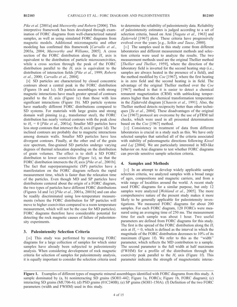
Pike et al. [2001a] andMuxworthy and Roberts [2006]. Thisinterpretive framework has been developed through exam-ination of FORC diagrams from well-characterized naturalsamples, as well as using simulated FORC diagrams frommagnetic models. Additional micromagnetic and othermodeling has confirmed this framework [Carvallo et al.,2003a, 2004; Muxworthy and Williams, 2005]. A crosssection of the FORC distribution along the Hc axis isequivalent to the distribution of particle microcoercivities,while a cross section through the peak of the FORCdistribution parallel to the Hi axis is equivalent to thedistribution of interaction fields [Pike et al., 1999; Robertset al., 2000; Carvallo et al., 2004].[9] SD particles are characterized by closed concentric

contours about a central peak in the FORC distribution(Figures 1b and 1c). SD particle assemblages with strongmagnetic interactions have much greater spread of contoursparallel to the Hi axis (Figure 1c) than those with lesssignificant interactions (Figure 1b). MD particle systemshave markedly different FORC distributions compared toSD systems. For materials with large grains and strongdomain wall pinning (e.g., transformer steel), the FORCdistribution has nearly vertical contours with the peak closeto Hc = 0 [Pike et al., 2001a]. Smaller MD particles haveless steep contours that intersect the Hi axis (Figure 1d). Theinclined contours are probably due to magnetic interactionsamong domain walls. Smaller MD particles have lessdivergent contours. Finally, at the other end of the grainsize spectrum, fine-grained SD particles undergo varyingdegrees of thermal relaxation depending on the distributionof grain volumes. The effect is to shift a SD FORCdistribution to lower coercivities (Figure 1e), so that theFORC distribution intersects the Hi axis [Pike et al., 2001b].The fact that superparamagnetic (SP) particles have amanifestation on the FORC diagram reflects the rapidmeasurement time, which is faster than the relaxation timeof the particles. Even though MD and SP particles havedistributions centered about the origin of a FORC diagram,the two types of particles have different FORC distributions(Figures 1d and 1e) [Pike et al., 2001a, 2001b] and can alsobe readily discriminated using low-temperature measure-ments (where the FORC distribution for SP particles willmove to higher coercivities compared to a room temperaturemeasurement, which will not be the case for MD particles).FORC diagrams therefore have considerable potential fordetecting the rock magnetic causes of failure of paleointen-sity experiments.

3. Paleointensity Selection Criteria

[10] This study was performed by measuring FORCdiagrams for a large collection of samples for which sistersamples have already been subjected to paleointensityanalysis. When considering development of rock magneticcriteria for selection of samples for paleointensity analysis,it is equally important to consider the selection criteria used

to determine the reliability of paleointensity data. Reliabilityof paleointensity estimates is judged according to a set ofselection criteria, based on Arai [Nagata et al., 1963] andZijderveld [1967] plots. These criteria have progressivelyevolved over the years [e.g., Selkin and Tauxe, 2000].[11] The samples used in this study come from different

laboratories and different measurement methods and selec-tion criteria were used to analyze the results. The twomeasurement methods used are the original Thellier method[Thellier and Thellier, 1959], where the direction of thelaboratory field is inverted for the second heating step (i.e.,samples are always heated in the presence of a field), andthe method modified by Coe [1967], where the first heatingis in zero field and the second heating is in field. Theadvantage of the original Thellier method over the Coe[1967] method is that it is easier to detect a chemicalremanent magnetization (CRM) with unblocking temper-atures higher than the chemical transformation temperaturein the Zijderveld diagram [Chauvin et al., 1991]. Also, theThellier method detects reciprocity better than other techni-ques [Yu et al., 2004]. These disadvantages of the originalCoe [1967] protocol are overcome by the use of pTRM tailchecks, which were used in all presented determinationsbased on the Coe [1967] method.[12] Consistency in treatment of data from different

laboratories is crucial in a study such as this. We have onlyselected samples that satisfied all of the criteria associatedwith stability of paleomagnetic directions following Kisseland Laj [2004]. We are particularly interested in MD-likebehavior on Arai diagrams to test whether FORC diagramscan provide sensitive sample selection criteria.

4. Samples and Methods

[13] In an attempt to develop widely applicable sampleselection criteria, we analyzed samples with a broad rangeof ages, compositions and magnetic carriers, and from awide range of localities around the world. A recent studyused FORC diagrams for a similar purpose, but only 12samples were analyzed [Wehland et al., 2005]. The morecomprehensive nature of the present study makes it morelikely to be generally applicable for paleointensity inves-tigations. We measured FORC diagrams for about 200samples. For each FORC diagram, 120 FORCs were mea-sured using an averaging time of 250 ms. The measurementtime for each sample was about 1 hour. Two usefulparameters are defined from FORC diagrams for this study.The first is the spread of the FORC distribution along the Hi

axis at Hc = 0, which is defined as the interval in which themagnitude of the FORC distribution decreases to 10% of itsmaximum (Figure 1f). We refer to this as the ‘‘width’’parameter, which reflects the MD contribution to a sample.The second parameter is the full width at half maximum(FWHM) for a profile of the distribution through thecoercivity peak parallel to the Hi axis (Figure 1f). Thisparameter indicates the strength of magnetostatic interac-

Figure 1. Examples of different types of magnetic mineral assemblages identified with FORC diagrams from this study. Asample dominated by (a, b) noninteracting SD grains (SOH1-442; Figure 1a, FORCs; Figure 1b, FORC diagram); (c)interacting SD grains (MU706-6); (d) PSD grains (01C240B); (e) SP grains (SOH1-150A). (f) Definition of the two FORCparameters (width and FWHM) used in this study.


4 of 15

B12103

tions within a sample. It should be noted that the FORCdistribution is least rigorously calculated along the Hc = 0axis because data cannot be obtained for Hc < 0, so thesmoothing associated with the polynomial used to calculatethe FORC distribution must be relaxed near Hc = 0 [Robertset al., 2000]. Despite possible distortion of the FORCdistribution in this part of the FORC diagram, we havepreferred to define the width parameter here (Figure 1f)because it best captures the vertical spread of contoursassociated with MD particles.[14] Half of the analyzed samples are from the Hawaiian

Scientific Drilling Project (HSDP) and Scientific Observa-tion Hole (SOH) numbers 1 and 4 on Kilauea volcano,Hawaii. Paleointensity analyses were performed on SOH1samples by Teanby et al. [2002], with a 70% success rate.SOH4 basalts also gave good paleointensity results, with a40% success rate [Laj et al., 2002]. Both SOH cores coverthe last 100 kyr. The HSDP core spans the last 420 kyr andwas drilled in the Mauna Loa and Mauna Kea volcanicseries. Paleointensity measurements for the HSDP core hada 75% success rate [Laj and Kissel, 1999]. The paleointen-sity results from the three cores together with paleodirectiondeterminations, carried out at the Laboratoire des Sciencesdu Climat et de l’Environnement paleomagnetic laboratoryin Gif-sur-Yvette, France, allowed detailed analysis ofgeomagnetic field behavior for the 0–420 kyr time interval.[15] Further samples analyzed in this study were collected

from localities around the world from rocks and potsherdsof a wide range of ages (Table 1). Samples were subjectedto absolute paleointensity analysis in the paleomagneticlaboratories of the Ludwig-Maximilians University,Munich, Germany, and of the University of Montpellier,France. Paleointensity determinations for the samples ana-lyzed in Munich included pTRM tail checks as well asadditivity checks [Krasa et al., 2003] in order to detect MDbehavior by checking the validity of Thellier’s law ofadditivity. The combination of pTRM checks and additivitychecks allows discrimination between magnetic mineralalteration and MD bias, therefore the alteration correctionof Valet et al. [1996] can be applied in appropriate cases[Leonhardt et al., 2003]. However, MD behavior identifiedat high temperature could also be a product of thermalalteration, and might not indicate the domain structure of theoriginal magnetic carrier, which is what matters for a correctpaleointensity determination. Any alteration correctionsmust therefore be applied with care. The paleointensityresults were analyzed using the ThellierTool software of

Leonhardt et al. [2004]. The other samples analyzed in thisstudy are described below in the following sections. Theresults described below are organized according to differentrelationships observed in FORC diagrams and Arai plotsregardless of sample locality and age.

5. Paleointensity Data and FORC Diagrams

5.1. Clear Correlation Between Paleointensity Resultsand FORC Diagrams

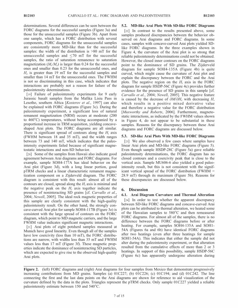
[16] Basalt samples from Mexico have a consistent trendbetween Arai plots and FORC diagrams. We analyzed 13samples from the early eruptive stage of the Trans-MexicanVolcanic Belt. The lavas erupted between 11 and 7 Ma andwere sampled from the Pacific coast to the longitude ofMexico City, to the north of the modern volcanic arc[Ferrari et al., 1999]. Paleointensity determinations weremade using the Thellier method. The resulting Arai plots areall more or less concave-curved (Figure 2). According to thecriteria of Selkin and Tauxe [2000], the least curved Araiplot still provides a reliable paleointensity estimate. Thelines shown on the Arai plots do not represent the fits usedto estimate the paleofield intensity. Rather, they connect thefirst and the last data points on the plots in order to aidvisualization of the curvature of the Arai plots.[17] FORC diagrams range from being SD-like, with

closed inner contours and little spread along the Hi axis(Figure 2a), to being more MD-like, with progressivelymuch larger spread of the outer contours, less closed innercontours, and a smaller tail toward high coercivities(Figure 2d). However, the coercivities associated with thepeaks of the FORC distributions do not vary significantly.The amount of curvature of the outer contours clearlycorrelates to the amount of spreading along the Hc = 0 axis,which is a measure of the MD contribution to the sample[Pike et al., 2001a]. For the four examples shown in Figure 2,the width of the distribution along the Hc = 0 axis (seeFigure 1f) increases progressively from 93 to 159 mT. Thissuggests that the progressively increasing curvature on theAraiplots is a result of increased contributions from MD grains.[18] The 8 studied samples from Amsterdam Island

(Indian Ocean) also have a clear relationship betweenFORC diagrams and paleointensity behavior. Completepaleointensity results, magnetic properties and radiometricage determinations for the analyzed samples are describedby Carvallo et al. [2003b]. These samples gave high-qualitypaleointensity determinations, with a success rate of 50%.Out of the 8 studied samples, 6 gave reliable paleointensity

Table 1. Summary of Samples Analyzed in This Study

Sample Location Age LithologySuccessfulSamples

FailedSamples Method Laboratory Reference

SOH1 Hawaii 20–120 kyr tholeiite 29 20 Thellier Gif-sur-Yvette Teanby et al. [2002]SOH4 Hawaii 0–100 kyr tholeiite 22 18 Thellier Gif-sur-Yvette Laj et al. [2002]HSDP Hawaii 0–420 kyr tholeiite 12 18 Thellier Gif-sur-Yvette Laj and Kissel [1999]98C Amsterdam Island 9–41 kyr tholeiite 6 2 Thellier Montpellier Carvallo et al. [2003b]92M Lesotho 180 Ma tholeiite 0 9 Thellier Montpellier Kosterov et al. [1997]01C Mexico 7–11 Ma andesitic basalt 1 12 Thellier Montpellier

Sao Tome 1–5 Ma alkali basalt 10 9 Coe MunichNazca 1.5 kyr potsherds 8 0 Coe MunichTenerife 6 Ma alkali basalt 2 5 Coe Munich Leonhardt and Soffel [2006]Hawaii 1 Ma tholeiite 0 6 Coe MunichBrazil 3 Ma alkali basalts 2 0 Coe Munich Leonhardt et al. [2003]


5 of 15

B12103

Figure 2


6 of 15

B12103

determinations. Several differences can be seen between theFORC diagrams for the successful samples (Figure 3a) andthose for the unsuccessful samples (Figure 3b). Apart fromone sample, which has a FORC distribution with severalcomponents, FORC diagrams for the unsuccessful samplesare consistently more MD-like than for the successfulsamples: the width of the distribution is >80 mT for theunsuccessful samples and �70 mT for the successfulsamples, the ratio of saturation remanence to saturationmagnetization (Mr/Ms) is larger than 0.24 for the successfulones and smaller than 0.23 for the unsuccessful ones, andHc is greater than 19 mT for the successful samples andsmaller than 14 mT for the unsuccessful ones. The FWHMis not so discriminating in this case, which indicates thatinteractions are probably not a reason for failure of thepaleointensity determinations.[19] Failure of paleointensity experiments for 9 early

Jurassic basalt samples from the Mafika Lisiu Pass inLesotho, southern Africa [Kosterov et al., 1997] can alsobe explained with FORC diagrams (Figure 3c). During thepaleointensity experiment, a significant loss of naturalremanent magnetization (NRM) occurs at moderate (200to 460�C) temperatures, without being accompanied by aproportional increase in TRM acquisition, yielding concave-shaped Arai plots. The FORC diagrams are all similar.There is significant spread of contours along the Hi axis(FWHM between 18 and 35 mT), and the width rangesbetween 73 and 140 mT, which indicates that the paleo-intensity experiments failed because of significant magne-tostatic interactions and non-SD behavior.[20] Some of the samples from Hawaii also indicate good

agreement between Arai diagrams and FORC diagrams. Forexample, sample SOH4-177A has ideal behavior on theArai plot (Figure 3d), with a long linear portion, goodpTRM checks and a linear characteristic remanent magne-tization component on a Zijderveld diagram. The FORCdiagram is consistent with this result: almost all of thecontours are closed, spread along the Hi axis is minimal andthe negative peak on the Hi axis together indicate thepresence of noninteracting SD grains [cf. Carvallo et al.,2004; Newell, 2005]. The ideal rock magnetic properties ofthis sample are clearly consistent with the high-qualitypaleointensity result. On the other hand, the strongly con-cave-curved Arai plot for sample SOH4-117B (Figure 3e) isconsistent with the large spread of contours on the FORCdiagram, which point to MD magnetic carriers, and the largeFWHM value indicates significant magnetic interactions.[21] Arai plots of eight potsherd samples measured at

Munich have good linearity. Even though all of the sampleshave low coercivity (less than 10 mT), the FORC distribu-tions are narrow, with widths less than 35 mT and FWHMvalues less than 17 mT (Figure 3f). These magnetic prop-erties indicate the dominance of noninteracting SD particles,which are expected to give rise to the observed high-qualityArai plots.

5.2. MD-like Arai Plots With SD-like FORC Diagrams

[22] In contrast to the results presented above, somesamples produced discrepancies between the behavior ob-served on Arai diagrams and FORC diagrams. In somecases, samples with concave-curved Arai plots yielded SD-like FORC diagrams. In the three examples shown inFigure 4, the curvature of the Arai plot is so strong thatreliable paleointensity determinations could not be obtained.However, the closed inner contours on the FORC diagramspoint to the dominance of SD grains. The Zijdervelddiagram for sample SOH4-135A (Figure 4b) is quitecurved, which might cause the curvature of Arai plot andexplain the discrepancy between the FORC and the Araiplots. The negative region on the Hi axis in the FORCdiagram for sample HSDP-56C (Figure 4c) provides furtherevidence for the presence of SD grains in this sample [cf.Carvallo et al., 2004; Newell, 2005]. This negative featureis caused by the decrease of @M/@Hr with decreasing H,which results in a positive mixed derivative valueand therefore a negative value for the FORC distribution[Muxworthy and Roberts, 2006]. Furthermore, magneto-static interactions, as indicated by the FWHM values shownin Figure 4, do not appear to be substantial in thesesamples. Reasons for the discrepancy between these Araidiagrams and FORC diagrams are discussed below.

5.3. SD-like Arai Plots With MD-like FORC Diagrams

[23] We also observed a few cases where samples havelinear Arai plots and MD-like FORC diagrams (Figure 5).Even though sample HSDP-28C (Figure 5a) gave reliablepaleointensity determinations, the FORC diagram has noclosed contours and a coercivity peak that is close to thevertical axis. Sample MU606-6 also yielded a good paleo-intensity result, but this is not consistent with the signif-icant vertical spread of the FORC distribution (FWHM =28.9 mT) through its maximum (Figure 5b). Reasons forthese discrepancies are discussed below.

6. Discussion

6.1. Arai Diagram Curvature and Thermal Alteration

[24] In order to test whether the apparent discrepancybetween SD-like FORC diagrams and concave-curved Araiplots can be attributed to thermal alteration, we heated someof the Hawaiian samples to 580�C and then remeasuredFORC diagrams. For almost all of the samples, there is nodifference between the FORC diagrams before or afterheating. For example, samples SOH4-135A and SOH1-54A (Figures 6a and 6b) have identical FORC diagramsafter two heatings (even after three heatings for sampleSOH1-54A). This indicates that either the sample did notalter during the paleointensity experiment, or that alterationresulted from the cumulative effects of more than 2 or 3heatings. In support of this possibility, sample HSDP-56C(Figure 6c) has apparently undergone alteration during

Figure 2. (left) FORC diagrams and (right) Arai diagrams for four samples from Mexico that demonstrate progressivelyincreasing contributions from MD grains. Samples (a) 01C227; (b) 01C226; (c) 01C194; and (d) 01C242. The lineconnecting the first and the last data points on the Arai diagrams are shown for reference to aid visualization of thecurvature defined by the data in the plots. Triangles represent the pTRM checks. Only sample 01C227 yielded a reliablepaleointensity estimate between 150 and 540�C.


7 of 15

B12103

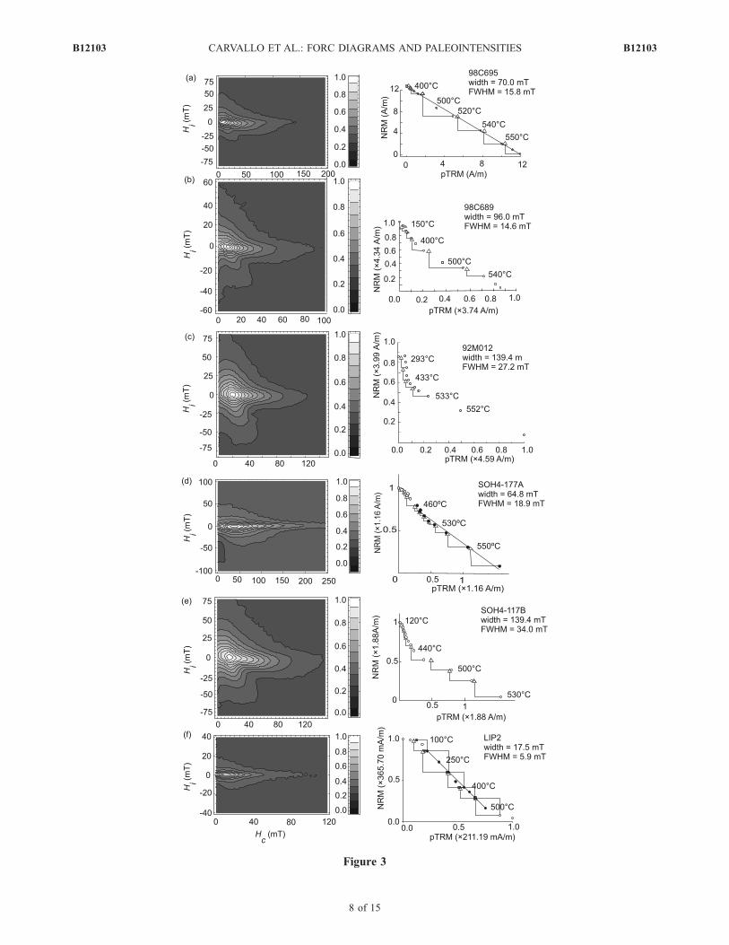
Figure 3


8 of 15

B12103

heating: the FORC distribution becomes more contractedalong both axes after progressive heating and the negativepeak that is evident in the pristine sample has almostdisappeared after the second heating.[25] In addition to analyzing samples that yielded con-

cave-curved Arai diagrams to test the effects of thermalalteration, we also heated and remeasured some samples forwhich the Arai plots indicate evidence of thermal alteration.However, the FORC diagrams after heating are similar to

those before heating. This result indicates that thermalalteration is difficult to detect with only a few heatings. Insome cases alteration occurs after only one heating, but inother cases it occurs after repeated heatings. The likelihoodof thermal alteration during the paleointensity experiment isoften assessed by examining the reversibility of Ms(T)curves, usually up to the Curie point. However, somesamples might alter at higher temperatures, but not at alower temperature range that would still give a reliable

Figure 3. (left) FORC diagrams and (right) Arai diagrams for samples with consistent behavior on the two diagrams. (a)Sample 98C695 (Amsterdam Island); (b) sample 98C689 (Amsterdam Island); (c) sample 92M012 (Lesotho); (d) sampleSOH4-177A (Hawaii); (e) sample SOH4-117B (Hawaii); and (f) sample LIP2 (Nazca). On the Arai plots, trianglesrepresent pTRM checks, and solid squares represent the pTRM tail checks on Figure 3f. The line on Figures 3a, 3d, and 3frepresent the best fits used for paleointensity estimates, the solid (open) symbols correspond to accepted (rejected) points.The other samples did not yield reliable paleointensity results.

Figure 4. (left) FORC diagrams and (right) Arai diagrams for samples with SD-like FORC diagramsand MD-like Arai diagrams. (a) Sample SOH1-54A (Hawaii); (b) sample SOH4-135A (Hawaii); and (c)sample HSDP-56C (Hawaii). On the Arai plots, triangles represent the pTRM checks. None of themyielded a reliable paleointensity estimate. The line connects the first and the last data points to aidvisualization of the curvature of the Arai plot.


9 of 15

B12103

paleointensity determination. Also, as we have shown here,alteration might occur after more than one heating. Thesefactors make it practically difficult to test for thermalalteration.[26] Another way of checking for thermal alteration is by

measuring a FORC diagram after a sample has beenanalyzed in a paleointensity experiment since this is thesample that has undergone heating at multiple steps. FORCdiagrams for 5 such samples from the HSDP core aremarkedly different from the FORC diagrams for the un-heated twin samples, which indicates that thermal alterationhas occurred. Sample HSDP-56C (Figure 6c) is a typicalexample: the FORC distribution after completion of thepaleointensity experiment is expanded along both axes. Theextent of the alteration is much more marked in the multiplyheated sample than after only one or two heatings. Thermalalteration could therefore be the cause of the curvature ofsome Arai plots despite the SD-like magnetic propertiesindicated by FORC diagrams for some samples (Figure 4).Unfortunately, only a small number of heated samples were

available after completion of paleointensity analysis, so wecould not systematically check for thermal alteration afterthe paleointensity measurement.

6.2. Sample Selection Criteria Based on FORCDiagrams

[27] Hysteresis parameters (e.g., Mrs/Ms and the ratio ofthe coercivity of remanence over the coercivity Hcr/Hc) areoften used to characterize domain structure. We have foundthat the parameters FWHM and width associated with theFORC distribution, as well as the coercive force Hc, aremuch more discriminating parameters than standard hyster-esis parameters represented on a Day plot [Day et al., 1977](Figure 7). Successful samples should have large Hc, smallwidth and small FWHM, to approximate ideal noninteract-ing SD magnetic properties. However, parts of the distribu-tions of these three parameters overlap for samples thatyielded successful and unsuccessful paleointensity results.This overlap partially results from the fact that magneticallyideal samples failed to produce high-quality paleointensityresults because of thermal alteration. However, the average

Figure 5. (left) FORC diagrams and (right) Arai diagrams for samples with MD-like FORC diagramsand SD-like Arai diagrams. (a) Sample HSDP-28C (Hawaii) and (b) sample MU606-6 (Brazil). On theArai plots, triangles represent the pTRM checks, the lines indicate the best fits used for paleointensityestimates, and the solid (open) symbols correspond to accepted (rejected) data points.


10 of 15

B12103

width of the FORC distribution for failed samples (86.1 mT)is higher than that of the successful samples (79.1 mT). Theaverage FWHM is also slightly higher for the failed samplescompared to the successful samples (20.2 mT compared to18.6 mT). Finally, the average Hc is only slightly lower forthe failed (18.2 mT) compared to the successful (19.5 mT)samples.[28] Statistically, the FWHM, width and Hc distributions

for successful and unsuccessful samples are not distinct.

However, only one third of the unsuccessful samples failedthe paleointensity experiment because of nonideal grain sizeor because of magnetic interactions. Two thirds of thesamples failed because of thermal alteration, thereforestatistics are not useful for assessing the distinctness ofour parameters.[29] However, in order to use FORC diagrams to develop

criteria for sample selection in paleointensity studies, weneed to set threshold values on these three parameters.

Figure 6. FORC diagrams measured at room temperature prior to any thermal treatment and afterheating for 20 min at 580�C. (a) Sample SOH4-135A; (b) sample SOH1-54A; and (c) FORC diagramsmeasured at room temperature prior to heating, after heating for 20 min at 580�C and after the fullpaleointensity experiment for sample HSDP-56C.


11 of 15

B12103

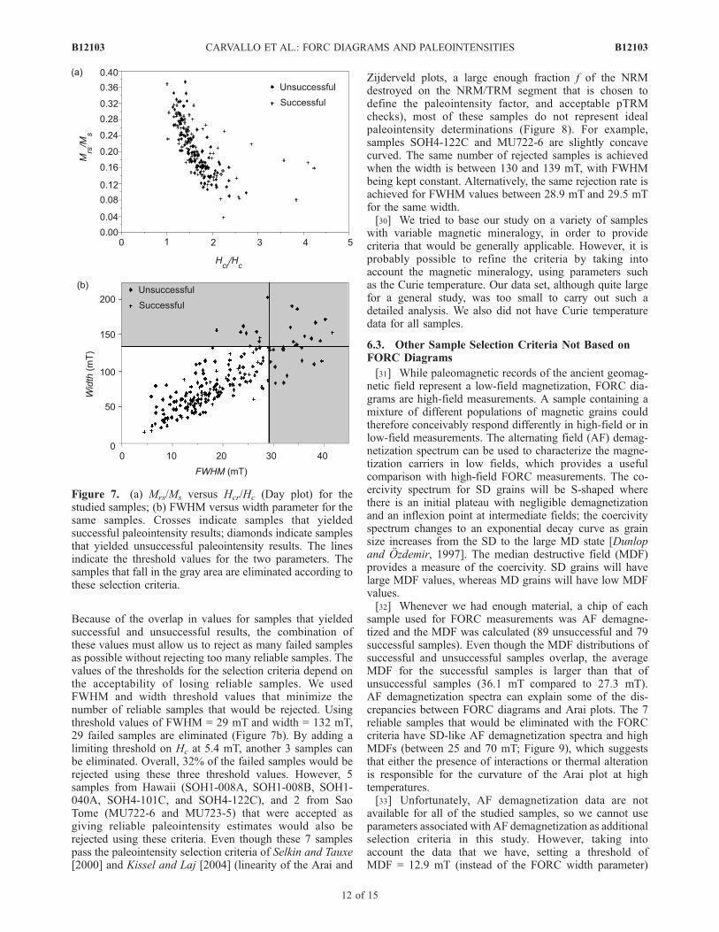
Because of the overlap in values for samples that yieldedsuccessful and unsuccessful results, the combination ofthese values must allow us to reject as many failed samplesas possible without rejecting too many reliable samples. Thevalues of the thresholds for the selection criteria depend onthe acceptability of losing reliable samples. We usedFWHM and width threshold values that minimize thenumber of reliable samples that would be rejected. Usingthreshold values of FWHM = 29 mT and width = 132 mT,29 failed samples are eliminated (Figure 7b). By adding alimiting threshold on Hc at 5.4 mT, another 3 samples canbe eliminated. Overall, 32% of the failed samples would berejected using these three threshold values. However, 5samples from Hawaii (SOH1-008A, SOH1-008B, SOH1-040A, SOH4-101C, and SOH4-122C), and 2 from SaoTome (MU722-6 and MU723-5) that were accepted asgiving reliable paleointensity estimates would also berejected using these criteria. Even though these 7 samplespass the paleointensity selection criteria of Selkin and Tauxe[2000] and Kissel and Laj [2004] (linearity of the Arai and

Zijderveld plots, a large enough fraction f of the NRMdestroyed on the NRM/TRM segment that is chosen todefine the paleointensity factor, and acceptable pTRMchecks), most of these samples do not represent idealpaleointensity determinations (Figure 8). For example,samples SOH4-122C and MU722-6 are slightly concavecurved. The same number of rejected samples is achievedwhen the width is between 130 and 139 mT, with FWHMbeing kept constant. Alternatively, the same rejection rate isachieved for FWHM values between 28.9 mT and 29.5 mTfor the same width.[30] We tried to base our study on a variety of samples

with variable magnetic mineralogy, in order to providecriteria that would be generally applicable. However, it isprobably possible to refine the criteria by taking intoaccount the magnetic mineralogy, using parameters suchas the Curie temperature. Our data set, although quite largefor a general study, was too small to carry out such adetailed analysis. We also did not have Curie temperaturedata for all samples.

6.3. Other Sample Selection Criteria Not Based onFORC Diagrams

[31] While paleomagnetic records of the ancient geomag-netic field represent a low-field magnetization, FORC dia-grams are high-field measurements. A sample containing amixture of different populations of magnetic grains couldtherefore conceivably respond differently in high-field or inlow-field measurements. The alternating field (AF) demag-netization spectrum can be used to characterize the magne-tization carriers in low fields, which provides a usefulcomparison with high-field FORC measurements. The co-ercivity spectrum for SD grains will be S-shaped wherethere is an initial plateau with negligible demagnetizationand an inflexion point at intermediate fields; the coercivityspectrum changes to an exponential decay curve as grainsize increases from the SD to the large MD state [Dunlopand Ozdemir, 1997]. The median destructive field (MDF)provides a measure of the coercivity. SD grains will havelarge MDF values, whereas MD grains will have low MDFvalues.[32] Whenever we had enough material, a chip of each

sample used for FORC measurements was AF demagne-tized and the MDF was calculated (89 unsuccessful and 79successful samples). Even though the MDF distributions ofsuccessful and unsuccessful samples overlap, the averageMDF for the successful samples is larger than that ofunsuccessful samples (36.1 mT compared to 27.3 mT).AF demagnetization spectra can explain some of the dis-crepancies between FORC diagrams and Arai plots. The 7reliable samples that would be eliminated with the FORCcriteria have SD-like AF demagnetization spectra and highMDFs (between 25 and 70 mT; Figure 9), which suggeststhat either the presence of interactions or thermal alterationis responsible for the curvature of the Arai plot at hightemperatures.[33] Unfortunately, AF demagnetization data are not

available for all of the studied samples, so we cannot useparameters associated with AF demagnetization as additionalselection criteria in this study. However, taking intoaccount the data that we have, setting a threshold ofMDF = 12.9 mT (instead of the FORC width parameter)

Figure 7. (a) Mrs/Ms versus Hcr/Hc (Day plot) for thestudied samples; (b) FWHM versus width parameter for thesame samples. Crosses indicate samples that yieldedsuccessful paleointensity results; diamonds indicate samplesthat yielded unsuccessful paleointensity results. The linesindicate the threshold values for the two parameters. Thesamples that fall in the gray area are eliminated according tothese selection criteria.


12 of 15

B12103

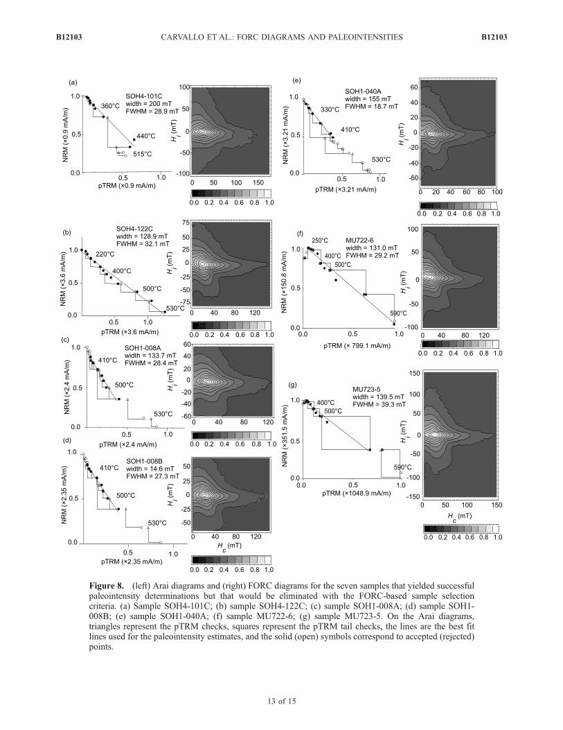
Figure 8. (left) Arai diagrams and (right) FORC diagrams for the seven samples that yielded successfulpaleointensity determinations but that would be eliminated with the FORC-based sample selectioncriteria. (a) Sample SOH4-101C; (b) sample SOH4-122C; (c) sample SOH1-008A; (d) sample SOH1-008B; (e) sample SOH1-040A; (f) sample MU722-6; (g) sample MU723-5. On the Arai diagrams,triangles represent the pTRM checks, squares represent the pTRM tail checks, the lines are the best fitlines used for the paleointensity estimates, and the solid (open) symbols correspond to accepted (rejected)points.


13 of 15

B12103

would allow us to reject 20 unsuccessful samples, withoutrejecting reliable samples, in addition to the 19 that arerejected using the FWHM interaction criterion. Togetherwith the 5 samples rejected using Hc, a total of 43% ofunsuccessful samples can be rejected using our preselec-tion criteria, while only rejecting 3 out of 94 reliablesamples. The MDF is more discriminating than the FORCdistribution width for detecting MD contributions to thelow field magnetization (NRM). However, AF demagneti-zation spectra cannot detect the presence of interactions, soFORC diagrams still represent a critical aspect of ourselection criteria.

7. Conclusions

[34] FORC diagrams were measured for 99 unsuccessfuland for 92 successful samples used for paleointensityexperiments. In general, the FORC diagrams for the suc-cessful samples are SD-like with minor to negligible inter-actions, while FORC diagrams for the unsuccessful samplesare more diverse. Unsuccessful samples could have failedthe paleointensity criteria because of thermal alteration,which is not detectable on a FORC diagram measured atroom temperature.[35] Selection criteria based on the FWHM of a vertical

profile through the maximum of the FORC distribution andon the width of the distribution along the Hc = 0 axis,provide a measure of interaction strength and of MDcontributions. Setting thresholds at 132 mT for width and29 mT for FWHM allows maximization of the number ofunsuccessful rejected samples and minimization of thenumber of successful rejected samples. With an additionalthreshold of Hc = 5.4 mT, 32 unsuccessful samples could berejected. Seven reliable samples (about 8%) would also berejected using these selection criteria. However, eventhough they satisfied the paleointensity selection criteria,these ‘‘reliable’’ samples did not represent ideal paleointen-sity determinations (Figure 8).[36] AF demagnetization spectra and the resultant MDFs

provide a measure of the MD contribution that might bemore discriminating of their contribution to the NRM thanthe FORC distribution width at Hc = 0. We were unable tomeasure AF demagnetization spectra for all of our samples,

but available data suggest that 43% of the unsuccessfulsamples can be eliminated (and only 3 reliable samples) if acriterion using a threshold value of 12.9 mT for MDF isused instead of the width of the FORC distribution.[37] Considering that thermal alteration is a major cause

of failure for paleointensity determinations and that itcannot be detected on FORC diagrams measured at roomtemperature, being able to eliminate at least one third of theunsuccessful samples with nonideal rock magnetic proper-ties (and potentially more than 40% of unsuccessful sam-ples) represents a significant improvement in paleointensitymeasurement time. It took about one hour to measure eachFORC diagram in this study, but it is possible to decreasethis time to 30 min for strongly magnetized material such asbasalts. The samples that failed because of the presence ofinteractions or MD behavior are efficiently detected usingFORC diagrams. Our sample selection criteria thereforeappear to have considerable promise for increasing theefficiency of absolute paleointensity studies.

[38] Acknowledgments. This research was funded by Marie CurieEC contract MCIF-CT-2004-0107843. We thank Jeff Gee and Ken Kodamafor constructive review comments that helped to improve the paper.

ReferencesCarter-Stiglitz, B., B. Moskowitz, and M. Jackson (2001), Unmixingmagnetic assemblages and the magnetic behavior of bimodal mixtures,J. Geophys. Res., 106, 26,397–26,411.

Carvallo, C., A. R. Muxworthy, D. J. Dunlop, and W. Williams (2003a),Micromagnetic modeling of first-order reversal curve (FORC) diagramsfor single-domain and pseudo-single-domain magnetite, Earth Planet.Sci. Lett., 213, 375–390.

Carvallo, C., P. Camps, G. Ruffet, B. Henry, and T. Poidras (2003b), MonoLake or Laschamps geomagnetic event recorded from lava flows in Am-sterdam Island (southeastern Indian Ocean), Geophys. J. Int., 154, 767–782.

Carvallo, C., O. Ozdemir, and D. J. Dunlop (2004), First-order reversalcurve (FORC) diagrams of elongated single-domain grains at high andlow temperatures, J. Geophys. Res., 109, B04105, doi:10.1029/2003JB002539.

Chauvin, A., P. Y. Gillot, and N. Bonhommet (1991), Paleointensity of theEarth’s magnetic field recorded by two late Quaternary volcanic se-quences at the island of La Reunion (Indian Ocean), J. Geophys. Res.,96, 1981–2006.

Cisowski, S. (1981), Interacting vs. non-interacting domain behavior innatural and synthetic samples, Phys. Earth Planet. Inter., 26, 56–62.

Coe, R. S. (1967), The determination of paleointensities of the Earth’smagnetic field with emphasis on mechanisms which could cause non-

Figure 9. AF demagnetization spectra for three successful samples that would have been rejected withthe FORC-based sample selection criteria.


14 of 15

B12103

ideal behavior in Thellier’s method, J. Geomagn. Geoelectr., 19, 157–179.

Cui, Y. L., K. L. Verosub, A. P. Roberts, and M. Kovacheva (1997), Mineralmagnetic criteria for sample selection in archaeomagnetic studies,J. Geomagn. Geoelectr., 49, 567–585.

Day, R., M. Fuller, and V. A. Schmidt (1977), Hysteresis properties oftitanomagnetites: Grain size and composition dependence, Phys. EarthPlanet. Inter., 13, 260–267.

Dunlop, D. J., and O. Ozdemir (1997), Rock Magnetism: Fundamentalsand Frontiers, 573 pp., Cambridge Univ. Press, New York.

Dunlop, D. J., and S. Xu (1994), Theory of partial thermoremanent mag-netization in multidomain grains: 1. Repeated identical barriers to wallmotion (single microcoercivity), J. Geophys. Res., 99, 9005–9023.

Dunlop, D. J., B. Zhang, and O. Ozdemir (2005), Linear and non-linearThellier paleointensity behavior of natural minerals, J. Geophys. Res.,110, B01103, doi:10.1029/2004JB003095.

Ferrari, L., M. Lopez-Martinez, G. Aguirre Diaz, and G. Carrasco Nunez(1999), Space-time patterns of Cenozoic arc volcanism in central Mexico:From the Sierra Madre Occidental to the Mexican volcanic belt, Geology,27, 303–306.

Kissel, C., and C. Laj (2004), Improvements in procedure and paleointen-sity selection criteria (PICRIT-03) for Thellier and Thellier determina-tions: Applications to Hawaiian basaltic long cores, Phys. Earth Planet.Inter., 147, 155–169.

Kosterov, A. A., M. Prevot, M. Perrin, and V. A. Shashkanov (1997),Paleointensity of the Earth’s magnetic field in the Jurassic: New resultsfrom a Thellier study of the Lesotho Basalt, southern Africa, J. Geophys.Res., 102, 24,859–24,872.

Krasa, D., C. Heunemann, R. Leonhardt, and N. Petersen (2003), Experi-mental procedure to detect multidomain remanence during Thellier-Thellier experiments, Phys. Chem. Earth, 28, 681–687.

Laj, C., and C. Kissel (1999), Geomagnetic field intensity at Hawaii for thelast 420 kyr from the Hawaii Scientific Drilling Project Core, Big Island,Hawaii, J. Geophys. Res., 104, 15,317–15,338.

Laj, C., C. Kissel, V. Scao, J. Beer, D. M. Thomas, H. Guillou, R. Muscheler,and G. Wagner (2002), Geomagnetic intensity and inclination variations atHawaii for the past 98 kyr from core SOH-4 (Big Island): A new study anda comparison with existing contemporary data, Phys. Earth Planet. Inter.,129, 205–243.

Leonhardt, R., and H. C. Soffel (2006), The growth, collapse and quies-cence of Teno volcano, Tenerife: New constraints from paleomagneticdata, Int. J. Earth Sci, in press.

Leonhardt, R., J. Matzka, and E. A. Menor (2003), Absolute paleointensi-ties and paleodirections from Fernando de Noronha, Brazil, Phys. EarthPlanet. Inter., 139, 285–303.

Leonhardt, R., C. Heunemann, and D. Krasa (2004), Analyzing absolutepaleointensity determinations: Acceptance criteria and the software Thel-lierTool4.0, Geochem. Geophys. Geosyst., 5, Q12016, doi:10.1029/2004GC000807.

Levi, S. (1977), The effect of magnetite particle size on paleointensitydeterminations of the geomagnetic field, Phys. Earth Planet. Inter., 13,245–259.

Muxworthy, A. R., and D. J. Dunlop (2002), First-order reversal curve(FORC) diagrams for pseudo-single-domain magnetites at high tempera-ture, Earth Planet. Sci. Lett., 203, 369–382.

Muxworthy, A. R., and A. P. Roberts (2006), First-order reversal curve(FORC) diagrams, in Encyclopedia of Geomagnetism and Paleomagnet-ism, edited by D. Gubbins, and E. Herrero-Bervera, Springer, New York,in press.

Muxworthy, A. R., and W. Williams (2005), Magnetostatic interactionfields in first-order-reversal-curve (FORC) diagrams, J. Appl. Phys., 97,063905.

Nagata, T., Y. Arai, and K. Momose (1963), Secular variation of the geo-magnetic total force during the last 5000 years, J. Geophys. Res., 68,5277–5281.

Newell, A. J. (2005), A high-precision model of first-order reversal curve(FORC) functions for single-domain ferromagnets with uniaxial aniso-tropy, Geochem. Geophys. Geosyst., 6, Q05010, doi:10.1029/2004GC000877.

Perrin, M. (1998), Paleointensity determination, magnetic domain structure,and selection criteria, J. Geophys. Res., 103, 30,591–30,600.

Perrin, M., and E. Schnepp (2004), IAGA paleointensity database: Distri-bution and quality of the data set, Phys. Earth Planet. Inter., 147, 255–267.

Pike, C. R., A. P. Roberts, and K. L. Verosub (1999), Characterizing inter-actions in fine magnetic particle systems using first order reversal curves,J. Appl. Phys., 85, 6660–6667.

Pike, C. R., A. P. Roberts, M. J. Dekkers, and K. L. Verosub (2001a), Aninvestigation of multi-domain hysteresis mechanisms using FORC dia-grams, Phys. Earth Planet. Inter., 126, 11–25.

Pike, C. R., A. P. Roberts, and K. L. Verosub (2001b), FORC diagrams andthermal relaxation effects in magnetic particles, Geophys. J. Int., 145,721–730.

Roberts, A. P., Y. L. Cui, and K. L. Verosub (1995), Wasp-waisted hyster-esis loops: Mineral magnetic characteristics and discrimination of com-ponents in mixed magnetic systems, J. Geophys. Res., 100, 17,909–17,924.

Roberts, A. P., C. R. Pike, and K. L. Verosub (2000), FORC diagrams: Anew tool for characterizing the magnetic properties of natural samples,J. Geophys. Res., 105, 28,461–28,475.

Selkin, P. A., and L. Tauxe (2000), Long-term variations in palaeointensity,Philos. Trans. R. Soc. London, 358, 1065–1088.

Teanby, N., C. Laj, D. Gubbins, and M. Pringle (2002), A detailed paleoin-tensity and inclination record from drill core SOH1 on Hawaii, Phys.Earth Planet. Inter., 131, 101–140.

Thellier, E. (1938), Sur l’aimantation des terres cuites et ses applicationsgeophysiques, Ann. Inst. Phys. Globe Univ. Paris, 16, 157–302.

Thellier, E., and O. Thellier (1959), Sur l’intensite du champ magnetiqueterrestre dans la passe historique et geologique, Ann. Geophys., 15, 285–376.

Thomas, D. N. (1993), An integrated rock magnetic approach to the selec-tion or rejection of ancient basalt samples for palaeointensity experi-ments, Phys. Earth Planet. Inter., 75, 329–342.

Valet, J. P., J. Brassart, I. Le Meur, V. Soler, X. Quidelleur, E. Tric, and P. Y.Gillot (1996), Absolute paleointensity and magnetomineralogicalchanges, J. Geophys. Res., 101, 25,029–25,055.

Wehland, F., R. Leonhardt, F. Vadeboin, and E. Appel (2005), Magneticinteraction analysis of basaltic samples and pre-selection for absolutepalaeointensity measurements, Geophys. J. Int., 162, 315–320.

Yu, Y., L. Tauxe, and A. Genevey (2004), Toward an optimal geomagneticfield intensity determination technique, Geochem. Geophys. Geosyst., 5,Q02H07, doi:10.1029/2003GC000630.

Zijderveld, J. D. A. (1967), AC demagnetization of rocks: Analysisof results, in Methods in Paleomagnetism, edited by D. W. Collinson,K. M. Creer, and S. K. Runcorn, pp. 254–386, Elsevier, New York.

��P. Camps and M. Perrin, Laboratoire Tectonophysique, CNRS and

Universite Montpellier II, Case 049, F-34095 Montpellier, France.C. Carvallo, Institut de Mineralogie et de Physique de la Matiere

Condensee, Universite Pierre et Marie Curie, Campus Boucicaut, 140 ruede Lourmel, F-75015 Paris, France. ([email protected])C. Kissel and C. Laj, Laboratoire des Sciences du Climat et de

l’Environnement, Unite Mixte CEA-CNRS, F-91198 Gif-sur-Yvette,France.R. Leonhardt, Department for Earth and Environmental Sciences,

Geophysics Section, Ludwig-Maximilians-Universitat Munchen, D-80333Munich, Germany.A. P. Roberts, National Oceanography Centre, University of South-

ampton, European Way, Southampton SO14 3ZH, UK.


15 of 15

B12103

Documents

Increasing the efficiency of paleointensity analyses by