INCREASING THE DAILY THROUGHPUT OF ECHOCARDIOGRAM PATIENTS ... · ii Title: Increasing the Daily Throughput of Echocardiogram Patients using Discrete Event Simulation Degree: Master

INCREASING THE DAILY THROUGHPUT OF

ECHOCARDIOGRAM PATIENTS USING DISCRETE

EVENT SIMULATION

by

Ronak Gandhi

A thesis submitted in conformity with the requirements

for the degree of Master of Health Science

Institute of Biomaterials and Biomedical Engineering

University of Toronto

© Copyright by Ronak Gandhi (2013)

ii

Title: Increasing the Daily Throughput of Echocardiogram Patients

using Discrete Event Simulation

Degree: Master of Health Science, 2013

Author: Ronak Gandhi

Department: Institute of Biomaterials and Biomedical Engineering

University: University of Toronto

ABSTRACT

Appointment scheduling involves picking a strategy for sequencing patient appointments such

that the wait time per patient is minimized and the idle time and overtime for the doctor are

minimized. The goal of this project is to increase the number of scans per day at the

echocardiogram clinic in the Hospital for Sick Children. The objectives were realized by

performing simulations of the workflow of the echo clinic using simulation software. The

simulation model did not precisely reflect the echo clinic, and the disparity was attributed to

limitations in the simulation model. Nevertheless, the user accepted the model and six different

policy change scenarios were explored. All six scenarios yielded significant increases in average

scans per day per sonographer. Scenario IV, which eliminated the use of sonographer schedules,

was recommended to be implemented due to ease of implementation and lack of negative effect

on patient wait time and sonographer overtime.

iii

ACKOWLEDGEMENTS

I would like to thank Professor Carter for all his patience, wisdom, and support throughout this

entire process. I would also like to thank the Centre for Research in Healthcare Engineering for

all of their insightful and stimulating discussion. I am particularly grateful for the guidance that

was given on useful tips for the simulation software.

I would also like to thank the staff at the echocardiogram clinic at Sick Kids Hospital for their

support during the data collection phase. I would especially like to acknowledge Dr. Luc Mertens

for being extremely supportive of the project and advocating its value to the rest of the clinic

management and physicians.

Lastly, I would like to thank my family and friends for all of their support throughout these past

couple of years.

iv

TABLE OF CONTENTS

1. INTRODUCTION ............................................................................................................................................ 1

OBJECTIVE .......................................................................................................................................................... 1 1.1

2. REVIEW OF LITERATURE ................................................................................................................................ 2

NUMBER OF DOCTORS .......................................................................................................................................... 2 2.1 NUMBER OF SERVICES ........................................................................................................................................... 3 2.2 LENGTH OF SERVICES ............................................................................................................................................ 3 2.3 ARRIVAL OF PATIENTS ........................................................................................................................................... 3 2.4 APPOINTMENT RULES ........................................................................................................................................... 4 2.5 PERFORMANCE MEASURES .................................................................................................................................... 5 2.6 SIMULATION CASE STUDIES .................................................................................................................................... 5 2.7

3. CURRENT STATE ............................................................................................................................................ 8

SICK KIDS ECHOCARDIOGRAM CLINIC ....................................................................................................................... 8 3.1 CURRENT APPOINTMENT RULES .............................................................................................................................. 9 3.2 CURRENT WORKFLOW DATA ................................................................................................................................ 10 3.3

4. SIMULATION MODEL .................................................................................................................................. 18

CONSTRUCTION OF SIMULATION MODEL ................................................................................................................ 18 4.1 SIMULATION VALIDATION .................................................................................................................................... 19 4.2

5. SIMULATIONS OF POLICY CHANGES ............................................................................................................ 25

RESULTS AND DISCUSSION ................................................................................................................................... 26 5.1

6. CONCLUSION AND FUTURE WORK .............................................................................................................. 32

7. REFERENCES ................................................................................................................................................ 34

8. APPENDIX A: SIMULATION MODEL ............................................................................................................. 36

v

LIST OF TABLES

TABLE 1. SONOGRAPHER OVERTIME CLAIMS IN 2011 .......................................................................................... 17

TABLE 2. COMPARISON OF OVERTIME CLAIMS .................................................................................................... 22

TABLE 3. DESCRIPTION OF POLICY CHANGES THAT WERE SIMULATED ................................................................. 25

TABLE 4. COMPARISON OF WHEN LATE PATIENTS ARE SCANNED IN SCENARIOS V & VI ...................................... 29

TABLE 5. SUMMARY OF RESULTS OBTAINED FROM SIMULATING DIFFERENT SCENARIOS ................................... 30

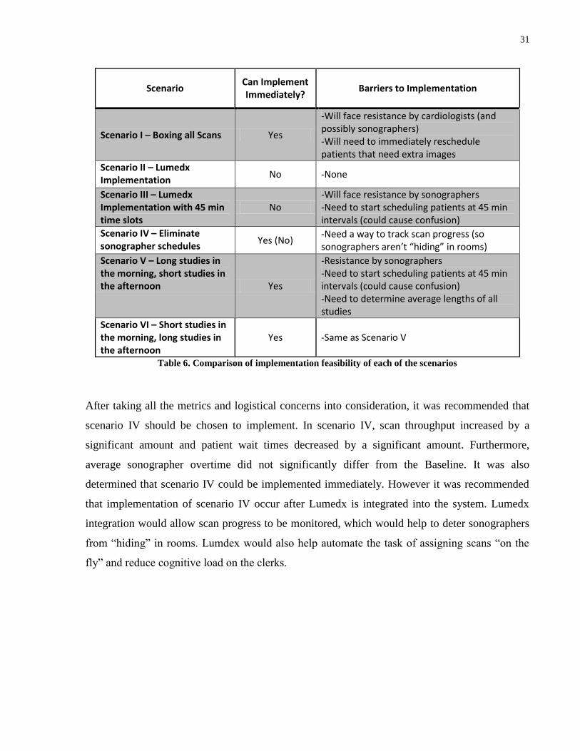
TABLE 6. COMPARISON OF IMPLEMENTATION FEASIBILITY OF EACH OF THE SCENARIOS .................................... 31

vi

LIST OF FIGURES

FIGURE 1. VISUALIZATION OF SELECTED APPOINTMENT RULES ............................................................................. 5

FIGURE 1. FLOWCHART OF PATIENT JOURNEY AT ECHO CLINIC FROM ARRIVAL TO EXIT ....................................... 8

FIGURE 2. TIMELINE OF SONOGRAPHERS’ ACTIVITY DURING THE 60 MINUTE APPOINTMENT SLOT ...................... 8

FIGURE 4. HISTOGRAM OF THE NUMBER OF ECHOCARDIOGRAM SCANS PERFORMED PER DAY PER SONOGRAPHER .................................................................................................................................................... 11

FIGURE 5. HISTOGRAM OF THE DURATION OF ECHOCARDIOGRAM SCANS. ......................................................... 11

FIGURE 6. HISTOGRAM OF THE TIME BETWEEN ECHOCARDIOGRAM SCANS FOR NON-ROVERS .......................... 12

FIGURE 7. HISTOGRAM OF THE TIME BETWEEN ECHOCARDIOGRAM SCANS FOR ROVERS ................................... 13

FIGURE 8. HISTOGRAM OF THE OUTPATIENT ARRIVAL TIMES .............................................................................. 14

FIGURE 9. HISTOGRAM OF THE OUTPATIENT WAIT TIMES ................................................................................... 14

FIGURE 10. HISTOGRAM OF THE SCAN REVIEW TIMES ......................................................................................... 15

FIGURE 11. HISTOGRAM OF THE SCAN REVIEW WAIT TIMES ............................................................................... 16

FIGURE 12. HISTOGRAM OF THE REPORT WRITING TIMES ................................................................................... 16

FIGURE 13. COMPARISON OF THE OUTPATIENT WAIT TIMES. .............................................................................. 19

FIGURE 14. COMPARISON OF THE AVERAGE WAIT TIME PER OUTPATIENT WHO EITHER EARLY OR ON TIME. .... 19

FIGURE 15. COMPARISON OF THE NUMBER OF ECHOCARDIOGRAM SCANS PERFORMED PER DAY PER SONOGRAPHER .................................................................................................................................................... 20

FIGURE 16. COMPARISON OF THE AVERAGE NUMBER OF ECHOCARDIOGRAM SCANS PERFORMED PER DAY PER SONOGRAPHER .................................................................................................................................................... 20

FIGURE 17. COMPARISON OF THE AVERAGE NUMBER OF INPATIENT ECHOCARDIOGRAM SCANS PERFORMED PER DAY PER SONOGRAPHER (NON-ROVER ONLY) .............................................................................................. 21

FIGURE 18. COMPARISON OF THE AVERAGE OVERTIME PERFORMED PER DAY PER SONOGRAPHER ................... 21

FIGURE 19. COMPARISON OF THE AVERAGE NUMBER OF ECHOCARDIOGRAM SCANS PERFORMED PER DAY PER SONOGRAPHER IN EACH OF THE SCENARIOS ....................................................................................................... 27

FIGURE 20. COMPARISON OF THE AVERAGE OUTPATIENT WAIT TIME IN EACH OF THE SCENARIOS .................... 28

FIGURE 21. COMPARISON OF THE AVERAGE SONOGRAPHER OVERTIMES IN EACH OF THE SCENARIOS .............. 29

1

1. INTRODUCTION

Patient wait times are extremely important in determining the success of a healthcare system. It

is not uncommon for patient wait times to be longer than their actual consultation times, where

the former may be over an hour, and the latter is usually 10-20mins [1]. Therefore it is not

surprising that much of the research in healthcare service operations has gone into the

improvement of appointment scheduling. This type of scheduling involves picking a strategy for

sequencing patient appointments such that the wait time per patient is minimized and the idle

time and overtime for the doctor are minimized. Patient wait time in this context is defined as the

time difference of the patient’s appointment time and when they are actually seen by the doctor

[2]. Idle time is defined as the time in which the doctor is not with a patient. This would occur if

patients arrive late to their appointment and the doctor is just waiting for them. Overtime is

defined as the amount of extra time a doctor has to stay past the regular clinic hours (e.g. 9am-

4pm). Wait time, idle time and over time have significant impact on the cost efficiency of a

clinic.

Objective 1.1

The purpose of this work is to evaluate the current situation at the echocardiogram clinic at the

Hospital for Sick Children. The goal of this project is to improve the efficiency of echo clinic

without increasing the number of resources (sonographers, doctors). Specifically, the goal is to

increase the number of scans per day. Furthermore, meeting this goal should have minimal

impact on other measures. Particularly, increases to patient wait time and sonographer overtime

should be minimized. In general, the number of scans per day should increase by a statistically

significant amount (p < 0.05), the idle time should decrease by a statistically significant amount,

and both the patient wait time and sonographer overtime should not increase a statistically

significant amount.

2

2. REVIEW OF LITERATURE

The goal of outpatient scheduling is to find an appointment scheduling system such that certain

measures of performance are optimized in a clinical environment [3]. This problem can be

thought of more generally as a subset of resource scheduling under uncertainty and can be

applied to a wide variety of environments, such as walk-in clinic patient scheduling, scheduling

patients for chemotherapy, radiology scheduling, operating room scheduling, etc.

Appointment scheduling can be broken down into two categories: static schedules and dynamic

schedules [3]. The static schedules are ones where the schedule is determined beforehand and

remains fixed throughout the duration of the day. Dynamic schedules are also determined

beforehand, but are subject to constant rescheduling if patients show up late or not at all. Most of

the literature involving appointment scheduling focuses on the static case, however some papers

have looked at the dynamic case as well [4, 5, 6, 7]. Overall, the primary factors that need to be

considered for both the static and dynamic cases include number of servers (doctors), number of

services (stages), length of services, and the arrival process of patients with regards to

punctuality and no shows. These factors and how they relate to the current circumstance at the

echo clinic will be discussed in more detail. Then we will discuss common appointment rules

used in modeling and common performance measures.

Number of Doctors 2.1

Most studies usually deal with clinics in which there is one server with multiple patients [3]. This

is akin to a situation where a patient needs to visit their family physician clinic. In this situation

there is one common queue for all patients and one server sees them one by one. As the number

of servers increases, it is still desirable to have one common queue for all patients; however,

clinics tend to use separate queues for each server. The reason for this is that patient-doctor

relationships are very important to the patient and they’d prefer to see the same doctor as they

did in their previous visit [3]. Although this would increase the wait times of patients, it would

also increase their satisfaction of the experience.

3

As mentioned previously, the echo lab has five sonographers that are available for all patients.

Although the schedules are made beforehand for each individual sonographer, any patient can

switch to another sonographer if the scheduler decides to do so. Therefore, sonographers can be

modeled as a five server system with a common queue. As for the two cardiologists, they

interpret the images after a sonographer finishes and may request a rescan. As such, cardiologists

do not usually interact with individual patients and can be modeled as a two server system with a

common queue.

Number of Services 2.2

Almost all the work done on appointment scheduling focuses on a single-stage model where

patients wait for a consultation with their doctor and then leave the clinic [3]. However there

have been studies which have investigated multi-stage models [8, 9, 10]. An example of a multi-

stage model would be where the patient has a test performed on them and the doctor has to

interpret the results and possibly redo the test. This is a two stage system and accurately reflects

the situation at the echo clinic.

Length of Services 2.3

Service time is defined as the time the server is with the patient [3]. Most appointment schedules

work with the assumption that each service time is equal for all patients and uniform throughout

the duration of the day, that is, service times are not expected to change as the day progresses.

This is similar to the situation at the echo lab. They indicate that the total service times last

between 30-60 min, with the variation strongly dependent on patient characteristics such as age,

medical condition, and type of scan requested. Therefore a service time distribution will have to

be determined empirically.

Arrival of Patients 2.4

The two main characteristics that concern the arrival of patients are punctuality and no-shows. In

a perfectly idealized model, the probability of either of these occurring would be null. However,

a high fidelity model would allow non-zero values of both. Punctuality is defined as the time

difference between their scheduled appointment time and the time they actually arrive and no-

4

shows are recorded at the end of the day if the patient did not arrive [3]. Empirical data suggest

that patients tend to arrive early for their appointment rather than late [7, 11, 12, 13, 14, 15].

When modeling patient punctuality, arrival distributions centered around patient appointment

times can be constructed from empirical data obtained from the clinic, however some authors

prefer to use theoretical probability distributions that have been fitted to empirically derived

histograms of patient arrival times [2, 9, 13, 16].

The probability of no-shows has also been investigated and values can range from 5 to 30

percent of scheduled patients per day [3]. A high probability of no-shows can have significant

impact on the efficiency of a clinic, as this can result in a significant increase of the doctors’ idle

time. For example, it was found that the no-show probability of patients has the greatest effect on

the efficiency of an appointment scheduling system [17]. Therefore, it is not surprising that there

has been much focus on determining variables that can affect patient attendance, and to identify

polices to discourage no-shows altogether. For instance, it was found that characteristics such as

patient age, gender, and even socioeconomic status can be helpful in predicting no-show

probability [18, 19]. Furthermore, Schafer suggests useful tips to deter patients from arriving late

or not at all, such as gently reminding patients of their appointment time if they were late, or

billing no-show patients if they are repeat offenders [20]. However, the latter may not be feasible

in a healthcare system in which fees for medically necessary services are covered by the

government.

Appointment Rules 2.5

The appointment rule is the primary characteristic of appointment scheduling. The rule is

essentially comprised of three variables: block size, initial block and appointment interval [1, 2,

3, 21]. The block size is defined as the number of patients scheduled for the same appointment

time, in most cases the block size is one. The initial block is the number of patients scheduled for

the first appointment of the day. The appointment interval is the interval between two

consecutive appointment times. This interval can be constant or variable.

Any combination of the above three variables can be an appointment rule. The most common

rule employed in clinics is the Individual-block/Fixed-Interval rule (IBFI). In this rule each

5

appointment block assigns only one patient and the interval between appointments is constant

and equal to the mean service time per patient. Another common tactic is to employ the IBFI rule

with an initial block. Bailey was the first to find that an IBFI rule with an initial block of two

patients would provide a good balance between patient wait time and server idle time [1, 3].

Classifying patients into subcategories can also be useful for employing more sophisticated

appointment rules [3]. Patients are usually classified as new or returning patients, but can even

be lumped together by age, medical condition or other attributes, such as type of procedure,

which would affect service time [22, 23, 24]. Classifying patients can be useful for rules that use

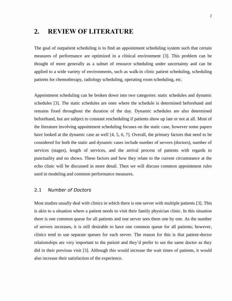
variable appointment intervals. Figure 1 is a visualization of the rules.

Figure 1. Visualization of selected appointment rules (visuals adopted from Cayirli & Veral) [3]

Performance Measures 2.6

There are many different metrics to evaluate the performance of an appointment schedule;

however they usually can all be reduced to a time-based measure [3]. In this measurement, there

are three important time variables that should be minimized: patient wait time, server idle time,

and server overtime.

Simulation Case Studies 2.7

Rule Visualization

IBFI

Bailey’s Rule where initial block is two

patients

Individual-Block/Variable-

interval

6

Simulating clinics on a case-by-case basis allows researchers and clinic management to

understand the relationship between appointment rules and their effect on clinic performance

measures. These case studies generally investigate specific real-life clinics, and therefore, a

major shortcoming of the findings from these studies is the lack of applicability to other more

general problems in outpatient appointment scheduling. Nevertheless, case studies have the

ability to offer valuable insight into the processes of real outpatient clinics.

One of the earliest studies in discrete-event outpatient simulation, performed by Fetter and

Thompson, analyzed physician utilization rates compared to patient wait time by experimenting

with various inputs (i.e. physician load, no-show rates, appointment scheduling intervals). They

determined that a 50% increase in physician load led to a significant decrease of physician idle

time and increase in patient wait time [13]. More specifically, patient wait times increased by 10

times the amount physician idle time decreased, from which the authors suggest that such a

capacity increase should only be done if physician time was at least 10 times more valuable than

patients’ time [13].

Another early study done by Williams, Covert and Steele investigated the use of a single block

appointment rule versus an IBFI appointment rule [25]. The single block rule does not specify

any appointment time and allows patients to show up anytime from when the clinic opens up

until it closes. It is the simplest type of appointment rule and one can imagine substantial patient

wait times if many patients (randomly) decided to arrive at approximately the same time. Their

study found that the single block rule yielded low physician idle times and the IBFI rule yielded

low patient wait times [25]. This study illustrates that when designing appointment rules, a

delicate balance must be struck between patient satisfaction and resource utilization.

Most of the existing literature on simulating real outpatient clinics focuses on reducing patient

wait times. However there are also studies which investigate the use of a simulation to increase

patient throughput. Centeno and Dodd perform a simulation study in order to increase the

throughput of patients at an endoscopy clinic. Although their simulation managed to show that a

30% increase in patient throughput would be possible, it came with the expense of hiring another

1.5 FTE nurse and adding a physician to two separate time slots [26]. Ramakrishnan et al.

present a simulation study aimed at increasing the throughput of patients at a radiology

7

department. They showed that adopting a digital image archiving system, along with creating

separate holding areas to perform preparatory activities before CT scanning, would increase

patient throughput by at least 20% [27]. However, this proposal also required significant capital

investment for purchasing the digital image archiving system, as well as the need to hire extra

personnel to operate the holding areas. The findings of these studies suggest that additional

resources may ultimately be required when attempting to increase patient throughput, and this is

generally not desirable given the current state of growing healthcare costs.

Another barrier to adopting authors’ recommendations from case studies is the medical

community’s resistance to change. The qualitative analysis on U.K. outpatient departments

performed by O’Keefe is a good example of how the underlying problem of appointment

scheduling can in fact be a political one. The author made recommendations for the

administrative staff to improve patient scheduling by proposing variable appointment durations

for new/follow-up patients, and made recommendations for physicians to start clinic hours on

time [11]. The first of these recommendations was rejected because those who scheduled

appointments were not expected to handle such complex appointment booking strategies. The

second recommendation was considered “unimplementable” because hospital management could

not enforce a change in the physicians’ behavior. A study conducted by Bennett and

Worthington also reported resistance by clinic staff when suggesting alternate operational

strategies to clinic staff [28]. Authors of both investigations concluded their papers by

highlighting the importance of proposing recommendations that are implementable, and urged

the inclusion of all stakeholders involved when designing strategies for improvement.

8

3. CURRENT STATE

Sick Kids Echocardiogram Clinic 3.1

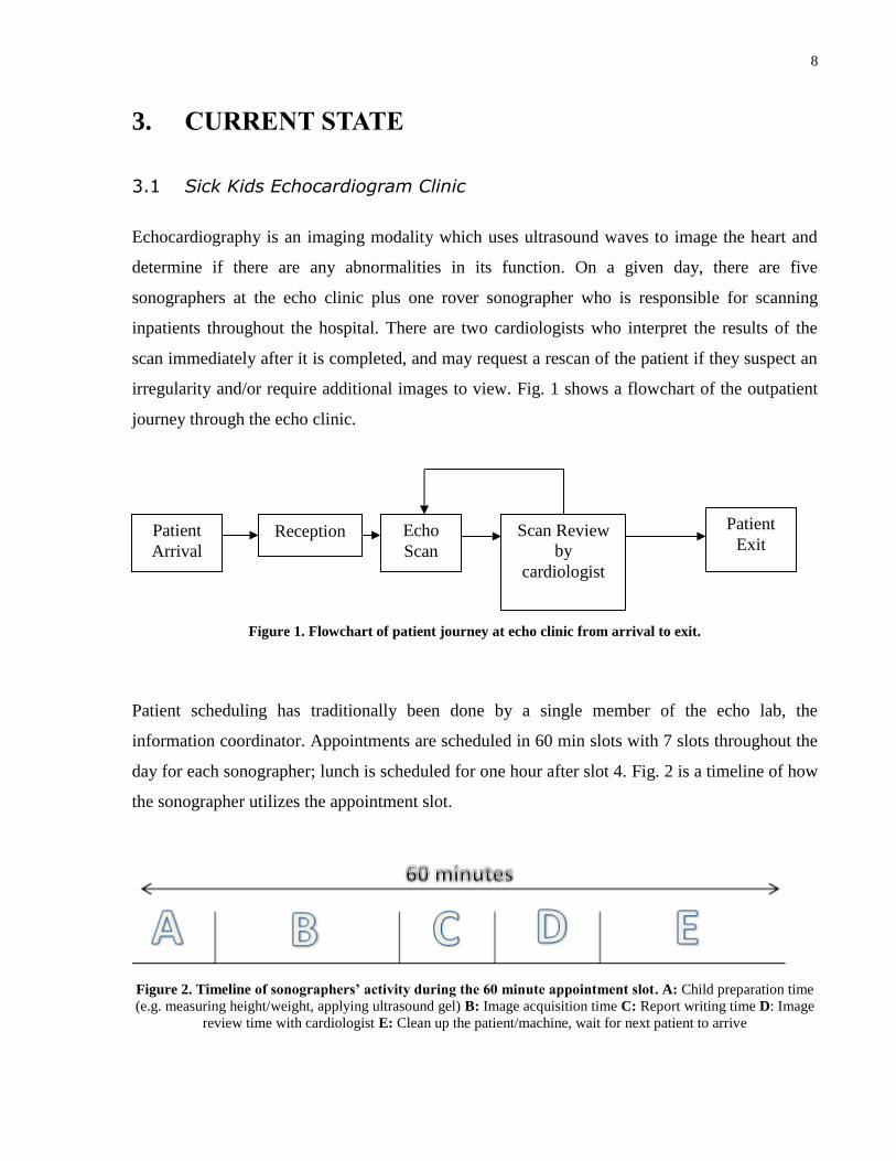
Echocardiography is an imaging modality which uses ultrasound waves to image the heart and

determine if there are any abnormalities in its function. On a given day, there are five

sonographers at the echo clinic plus one rover sonographer who is responsible for scanning

inpatients throughout the hospital. There are two cardiologists who interpret the results of the

scan immediately after it is completed, and may request a rescan of the patient if they suspect an

irregularity and/or require additional images to view. Fig. 1 shows a flowchart of the outpatient

journey through the echo clinic.

Figure 1. Flowchart of patient journey at echo clinic from arrival to exit.

Patient scheduling has traditionally been done by a single member of the echo lab, the

information coordinator. Appointments are scheduled in 60 min slots with 7 slots throughout the

day for each sonographer; lunch is scheduled for one hour after slot 4. Fig. 2 is a timeline of how

the sonographer utilizes the appointment slot.

Figure 2. Timeline of sonographers’ activity during the 60 minute appointment slot. A: Child preparation time

(e.g. measuring height/weight, applying ultrasound gel) B: Image acquisition time C: Report writing time D: Image

review time with cardiologist E: Clean up the patient/machine, wait for next patient to arrive

Patient

Arrival

Reception Echo

Scan

Scan Review

by

cardiologist

Patient

Exit

9

The scheduling of patients in each slot is done manually for each of the five sonographers,

usually the day before, and must be updated during the day if patients arrive late or not at all.

The scheduler must also be able to make adjustments for add-on and inpatient scans that have

priority. The goal of the scheduler is to shift around the schedule whenever there are late or no-

show patients, in order to maximize the number of patients seen per day (daily patient

throughput). This task is very cognitively demanding and the schedule that is decided on may not

even maximize daily patient frequency.

Current Appointment Rules 3.2

Sonographers have three possible shift times: 8am to 4pm, 8:30am to 4:30pm, or 9pm to 5pm.

Shifts are assigned by the scheduler for each sonographer one month in advance. For each

sonographer, all appointment slots are booked with outpatients except the last slot of the day.

This is intentionally left empty to deal with sonographer and/or patients running late throughout

the day. Therefore each sonographer has six patients booked for scanning each day, and the last

slot can be used to scan an inpatient if the sonographer has enough time to do so.

After the outpatients arrive, the receptionist sorts them into queues depending on their arrival

time relative to their appointment time. Patients who arrive early, defined as more than 30

minutes before their scheduled appointment time, are placed in the Early queue. Patients who

arrive late, defined as more than 5 minutes after their scheduled appointment time, are placed in

the Late queue. Patients who are not Early or Late are placed in the On Time queue.

Sonographers are given their appointment schedule at the beginning of the day. If every single

patient comes on time then sonographers will scan each patient that is listed in their schedule.

However, when patients arrive late or do not show, the sonographer does not spend time simply

waiting for their patient. Instead, if 5 minutes has passed after the scheduled appointment time

and their patient has not arrived then the sonographer must take another patient from a non-

empty queue. The rules for queue selection are as follows:

1. On Time patient who is still waiting

10

2. Earliest Late patient; Late patient who has been waiting the longest

3. Early patient

4. Inpatient; these patients are not booked ahead of time so it may be difficult

The rules essentially state that On Time patients get priority over all others and are seen first by

the next available sonographer. If there are no On Time patients waiting then the Late patient

who has been waiting the longest is next. If there are no Late patients then an Early patient is

scanned. If a patient is in the Early queue and their scheduled appointment time is in less than 30

minutes, they are automatically moved to the front of the On Time queue and will have first

priority when the next available sonographer becomes free. If there are no Early patients then the

sonographer must scan an inpatient.

Ideally, the inpatient would simply be able to come to the echo lab and be scanned. However, if

the patient is unable to do so, the sonographer must go to the patient’s room and perform the

scan there. This involves powering down the echocardiogram machine, travelling to the patient,

powering up the machine, performing the scan, powering down the machine again, travelling

back to the echo lab, and powering up the machine again. Since the sonographer needs to make it

back in time for their next scheduled appointment, inpatient scans should only be initiated if the

sonographer feels that scanning an inpatient will not keep their next scheduled patient waiting for

an unreasonably long time.

Current Workflow Data 3.3

In order to build the simulation, it was necessary to collect the preliminary data for the existing

workflow. The preliminary data included: number of scans per day (performance measure),

image acquisition times, time between image acquisitions, outpatient arrival times, outpatient

wait time (performance measure), sonographer idle and overtimes (performance measures), scan

review times, scan review wait times, report writing times.

The majority of the data were collected by conducting direct observations at the echo clinic.

However, image acquisition times, time between image acquisitions, and sonographer overtimes

were collected from the echocardiogram clinic computer database.

11

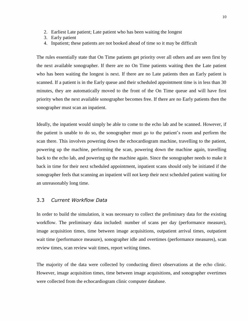
Figure 4. Histogram of the number of echocardiogram scans performed per day per sonographer

Fig. 4 shows the histogram of the number of echocardiogram scans performed per sonographer

per day. Since there are 7 one hour slots that are available for scanning, the echo clinic would be

at maximum efficiency if each sonographer performed 7 scans per day. The average number of

scans performed is approximately 5.5, which is 21% below maximum efficiency. This is a clear

indication that there is room for improvement in increasing patient throughput.

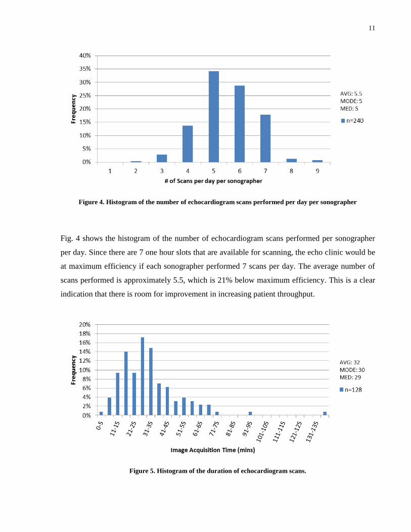
Figure 5. Histogram of the duration of echocardiogram scans.

12

Fig. 5 is a histogram of the duration of the echocardiogram scans. It should be noted that this

duration only represents the time between the acquisition of the first image to the last. This scan

duration does not include scan preparation time, the time to write the post scan report, or scan

review time with cardiologist. The average scan time is approximately 32 min, which indicates

that only about half the 60 min time slot is being used for scanning purposes.

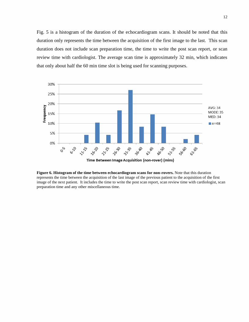
Figure 6. Histogram of the time between echocardiogram scans for non-rovers. Note that this duration

represents the time between the acquisition of the last image of the previous patient to the acquisition of the first

image of the next patient. It includes the time to write the post scan report, scan review time with cardiologist, scan

preparation time and any other miscellaneous time.

13

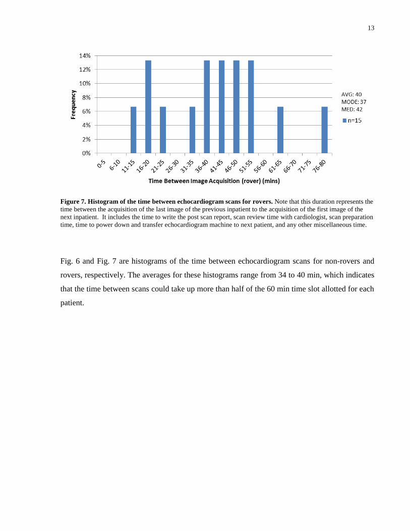
Figure 7. Histogram of the time between echocardiogram scans for rovers. Note that this duration represents the

time between the acquisition of the last image of the previous inpatient to the acquisition of the first image of the

next inpatient. It includes the time to write the post scan report, scan review time with cardiologist, scan preparation

time, time to power down and transfer echocardiogram machine to next patient, and any other miscellaneous time.

Fig. 6 and Fig. 7 are histograms of the time between echocardiogram scans for non-rovers and

rovers, respectively. The averages for these histograms range from 34 to 40 min, which indicates

that the time between scans could take up more than half of the 60 min time slot allotted for each

patient.

14

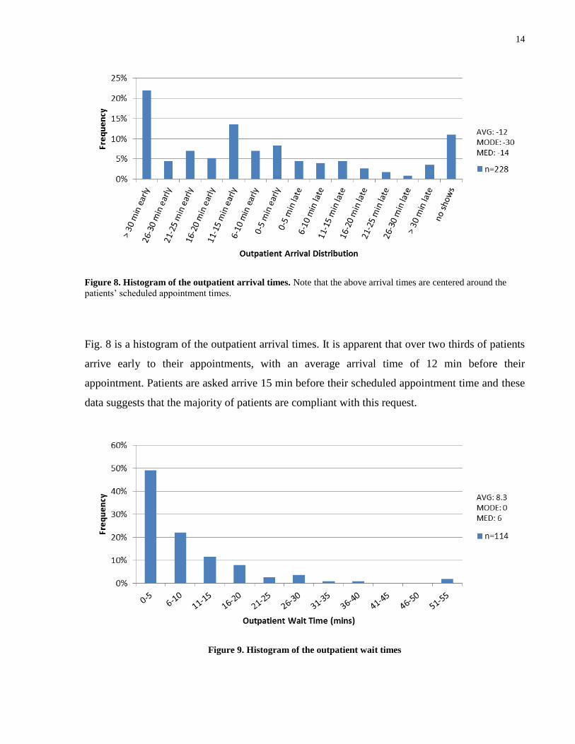
Figure 8. Histogram of the outpatient arrival times. Note that the above arrival times are centered around the

patients’ scheduled appointment times.

Fig. 8 is a histogram of the outpatient arrival times. It is apparent that over two thirds of patients

arrive early to their appointments, with an average arrival time of 12 min before their

appointment. Patients are asked arrive 15 min before their scheduled appointment time and these

data suggests that the majority of patients are compliant with this request.

Figure 9. Histogram of the outpatient wait times

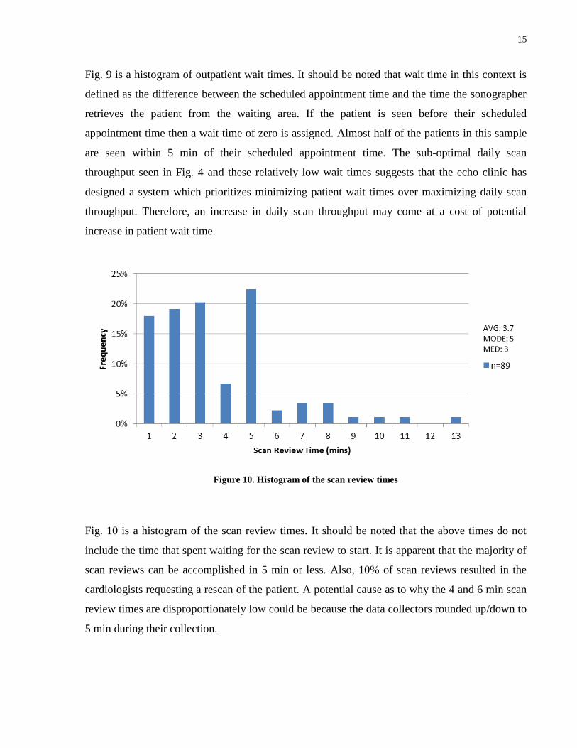
15

Fig. 9 is a histogram of outpatient wait times. It should be noted that wait time in this context is

defined as the difference between the scheduled appointment time and the time the sonographer

retrieves the patient from the waiting area. If the patient is seen before their scheduled

appointment time then a wait time of zero is assigned. Almost half of the patients in this sample

are seen within 5 min of their scheduled appointment time. The sub-optimal daily scan

throughput seen in Fig. 4 and these relatively low wait times suggests that the echo clinic has

designed a system which prioritizes minimizing patient wait times over maximizing daily scan

throughput. Therefore, an increase in daily scan throughput may come at a cost of potential

increase in patient wait time.

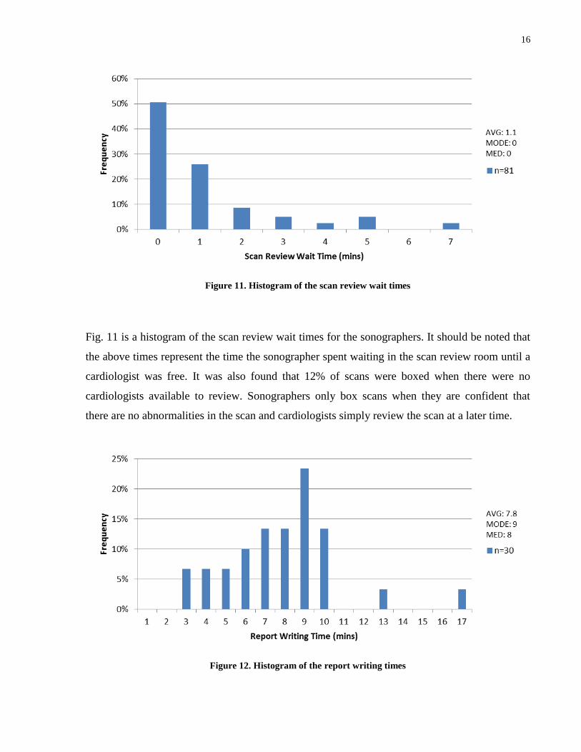
Figure 10. Histogram of the scan review times

Fig. 10 is a histogram of the scan review times. It should be noted that the above times do not

include the time that spent waiting for the scan review to start. It is apparent that the majority of

scan reviews can be accomplished in 5 min or less. Also, 10% of scan reviews resulted in the

cardiologists requesting a rescan of the patient. A potential cause as to why the 4 and 6 min scan

review times are disproportionately low could be because the data collectors rounded up/down to

5 min during their collection.

16

Figure 11. Histogram of the scan review wait times

Fig. 11 is a histogram of the scan review wait times for the sonographers. It should be noted that

the above times represent the time the sonographer spent waiting in the scan review room until a

cardiologist was free. It was also found that 12% of scans were boxed when there were no

cardiologists available to review. Sonographers only box scans when they are confident that

there are no abnormalities in the scan and cardiologists simply review the scan at a later time.

Figure 12. Histogram of the report writing times

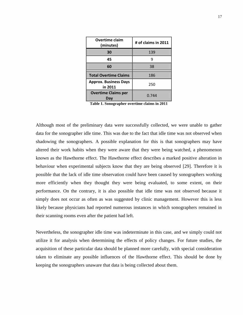
17

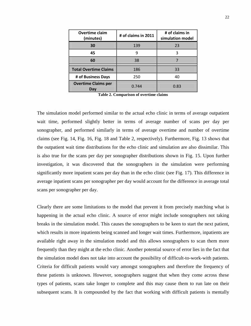
Overtime claim (minutes)

# of claims in 2011

30 139

45 9

60 38

Total Overtime Claims 186

Approx. Business Days in 2011

250

Overtime Claims per Day

0.744

Table 1. Sonographer overtime claims in 2011

Although most of the preliminary data were successfully collected, we were unable to gather

data for the sonographer idle time. This was due to the fact that idle time was not observed when

shadowing the sonographers. A possible explanation for this is that sonographers may have

altered their work habits when they were aware that they were being watched, a phenomenon

known as the Hawthorne effect. The Hawthorne effect describes a marked positive alteration in

behaviour when experimental subjects know that they are being observed [29]. Therefore it is

possible that the lack of idle time observation could have been caused by sonographers working

more efficiently when they thought they were being evaluated, to some extent, on their

performance. On the contrary, it is also possible that idle time was not observed because it

simply does not occur as often as was suggested by clinic management. However this is less

likely because physicians had reported numerous instances in which sonographers remained in

their scanning rooms even after the patient had left.

Nevertheless, the sonographer idle time was indeterminate in this case, and we simply could not

utilize it for analysis when determining the effects of policy changes. For future studies, the

acquisition of these particular data should be planned more carefully, with special consideration

taken to eliminate any possible influences of the Hawthorne effect. This should be done by

keeping the sonographers unaware that data is being collected about them.

18

4. SIMULATION MODEL

The simulation model was constructed after the preliminary data were collected. This was done

using SIMUL8™ software. After the simulation model was constructed, the model was validated

in order to justify that it was accurately representing the current workflow at the echo clinic. This

was done by comparing the data of the performance measures of the existing workflow to the

data of the performance measures that were obtained from the simulation.

Construction of Simulation Model 4.1

A discrete event simulation model was constructed based on the existing appointment rules and

statistics using SIMUL8™ software. This section will give an overview of the simulation model

and describe the validation results. For comprehensive details of the model’s structure, including

all visual logic code, please see Appendix A.

The model was based on the Monday, Tuesday, Wednesday clinic schedule. These days were

chosen to be represented by the model because the staffing requirements for these days are more

consistent than compared to the Thursday and Friday schedules. There are always a total of six

sonographers each day from Monday to Wednesday: five sonographers in the clinic plus one

rover. Three of the five sonographers plus the rover are on the 8am-4pm shift. Two sonographers

are on the 8:30am-4:30pm shift. There is usually no sonographer on the 9am-5pm shift on the

Monday to Wednesday.

Patient arrival was based on the distribution in Fig. 8. Patients are permitted to arrive up to 1

hour earlier than their appointment time and up to 1 hour late. Scan duration was based on the

distribution in Fig. 5. The distribution in Fig. 5 contained outliers; values larger than 75 minutes

were truncated and the resulting distribution was used. Report writing time was based on the

distribution in Fig. 12. Scan review time was based on the distribution in Fig. 10. The time

between image acquisitions for non-rovers was based on the distribution in Fig. 6, minus report

writing and scan review times. The time between image acquisitions for the rover is based on the

distribution in Fig. 7, minus report writing and scan review times. A more detailed breakdown of

the simulation model can be found in Appendix A.

19

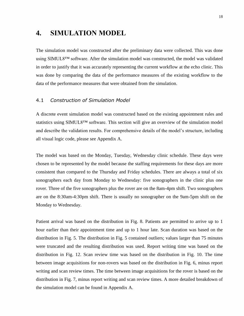
Simulation Validation 4.2

Figure 13. Comparison of the outpatient wait times. The histogram in Fig. 9 is plotted next to the results of the

outpatient wait time results obtained from the running the simulation.

Figure 14. Comparison of the average wait time per outpatient who either early or on time.

20

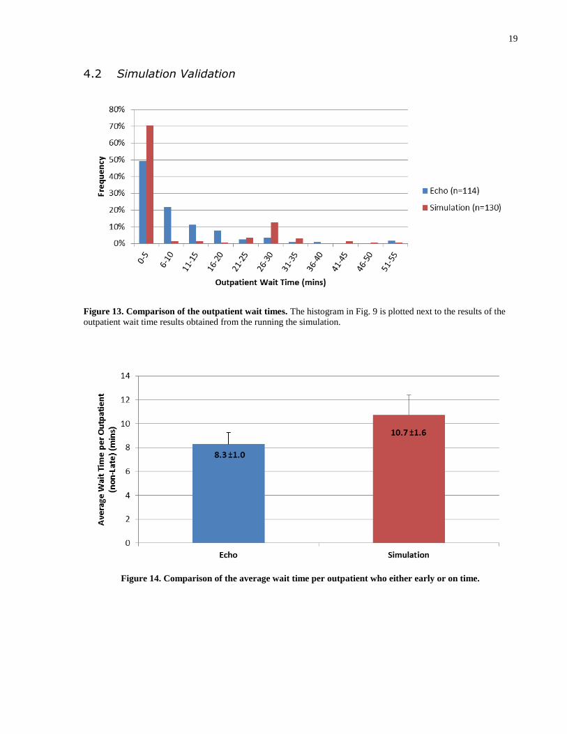
Figure 15. Comparison of the number of echocardiogram scans performed per day per sonographer. The

histogram in Fig. 4 is plotted next to the results of results obtained from the running the simulation.

Figure 16. Comparison of the average number of echocardiogram scans performed per day per sonographer *Denotes statistical significance via t-test (p < 0.05)

21

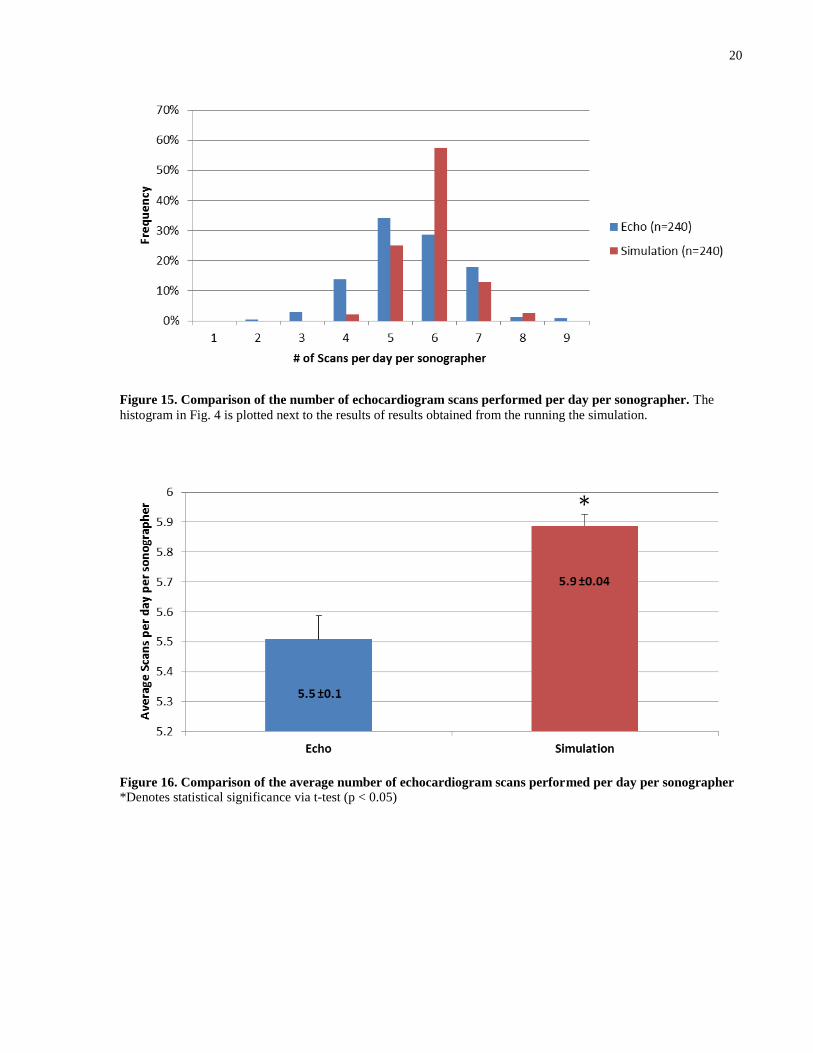
Figure 17. Comparison of the average number of inpatient echocardiogram scans performed per day per

sonographer (non-rover only). *Denotes statistical significance via t-test (p < 0.05)

Figure 18. Comparison of the average overtime performed per day per sonographer. *Denotes statistical

significance via t-test (p < 0.05)

22

Overtime claim (minutes)

# of claims in 2011 # of claims in

simulation model

30 139 23

45 9 3

60 38 7

Total Overtime Claims 186 33

# of Business Days 250 40

Overtime Claims per Day

0.744 0.83

Table 2. Comparison of overtime claims

The simulation model performed similar to the actual echo clinic in terms of average outpatient

wait time, performed slightly better in terms of average number of scans per day per

sonographer, and performed similarly in terms of average overtime and number of overtime

claims (see Fig. 14, Fig. 16, Fig. 18 and Table 2, respectively). Furthermore, Fig. 13 shows that

the outpatient wait time distributions for the echo clinic and simulation are also dissimilar. This

is also true for the scans per day per sonographer distributions shown in Fig. 15. Upon further

investigation, it was discovered that the sonographers in the simulation were performing

significantly more inpatient scans per day than in the echo clinic (see Fig. 17). This difference in

average inpatient scans per sonographer per day would account for the difference in average total

scans per sonographer per day.

Clearly there are some limitations to the model that prevent it from precisely matching what is

happening in the actual echo clinic. A source of error might include sonographers not taking

breaks in the simulation model. This causes the sonographers to be keen to start the next patient,

which results in more inpatients being scanned and longer wait times. Furthermore, inpatients are

available right away in the simulation model and this allows sonographers to scan them more

frequently than they might at the echo clinic. Another potential source of error lies in the fact that

the simulation model does not take into account the possibility of difficult-to-work-with patients.

Criteria for difficult patients would vary amongst sonographers and therefore the frequency of

these patients is unknown. However, sonographers suggest that when they come across these

types of patients, scans take longer to complete and this may cause them to run late on their

subsequent scans. It is compounded by the fact that working with difficult patients is mentally

23

draining on the sonographer. Since the simulation does not contain difficult patients, it can

potentially allow for more patients to be scanned per day compared to the echo clinic. Another

source of error could be with the receptionist in the simulation model. The receptionist in the

model queues patients instantly, which would allow patients to get into the waiting queue faster

which would allow them to be scanned more frequently. At the echo clinic, the receptionist often

performs other tasks along with registering patients which might delay them from being entered

into the queue.

Another limitation of the model is that all the sonographers were homogeneous. This resulted in

each sonographer having equivalent scan time distributions. This is potential source of error

because each sonographer in the echo clinic is unique and each would have their own unique

scan time distribution. Therefore, using homogeneous sonographers might skew the number of

scans that can be performed daily. Ideally, when modelling sonographers in the simulation

unique scan time distributions should be created for each sonographer.

The final limitation to the simulation is rooted in the fact that human sonographers have the

ability to make decisions and adjustments to their work pace, whereas the sonographers in the

simulation do not. For instance, if a human sonographer is early for their next patient they might

choose to scan the patient right away or take a quick break. Sonographers in the model do not

have the ability to make such decisions, and therefore fudge factors were included in the code. In

the model, sonographers will not take new outpatients 30 min before the start of their next

appointment and will not take new inpatients 40 min before the start of their next appointment.

Essentially, these fudge factors describe the phenomenon in which sonographers tend to “hide”

in their rooms until their next scheduled appointment, even if they have finished their last

appointment early. Furthermore, the fudge factors also allowed the simulation model to more

accurately reflect the number of scans per day being achieved at the echo clinic. However, the

fudge factors may also have contributed to longer wait times in the simulation model compared

to the echo clinic.

Nevertheless, despite all of the aforementioned limitations and sources of error in the model, it

was felt that the simulation could still provide valuable insight into the effects that might result

24

when policy changes occur. The limitations and sources of error were presented to the echo

clinic management and they too felt the model was acceptable.

25

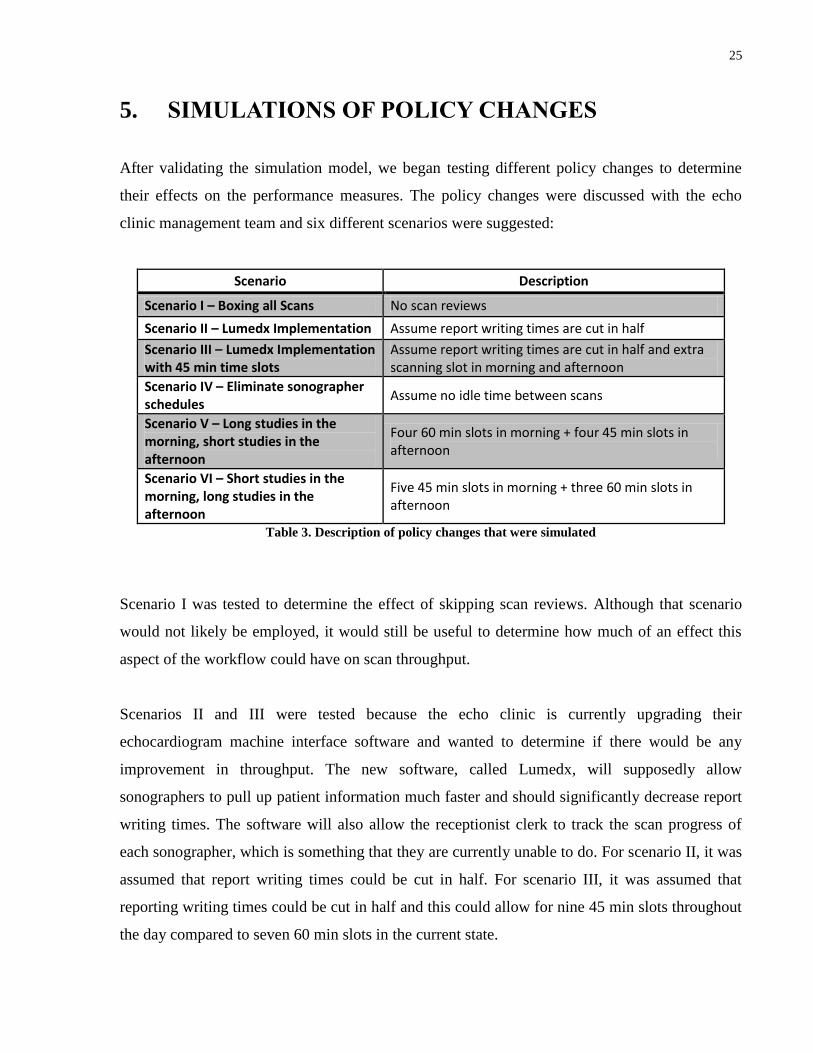
5. SIMULATIONS OF POLICY CHANGES

After validating the simulation model, we began testing different policy changes to determine

their effects on the performance measures. The policy changes were discussed with the echo

clinic management team and six different scenarios were suggested:

Scenario Description

Scenario I – Boxing all Scans No scan reviews

Scenario II – Lumedx Implementation Assume report writing times are cut in half

Scenario III – Lumedx Implementation with 45 min time slots

Assume report writing times are cut in half and extra scanning slot in morning and afternoon

Scenario IV – Eliminate sonographer schedules

Assume no idle time between scans

Scenario V – Long studies in the morning, short studies in the afternoon

Four 60 min slots in morning + four 45 min slots in afternoon

Scenario VI – Short studies in the morning, long studies in the afternoon

Five 45 min slots in morning + three 60 min slots in afternoon

Table 3. Description of policy changes that were simulated

Scenario I was tested to determine the effect of skipping scan reviews. Although that scenario

would not likely be employed, it would still be useful to determine how much of an effect this

aspect of the workflow could have on scan throughput.

Scenarios II and III were tested because the echo clinic is currently upgrading their

echocardiogram machine interface software and wanted to determine if there would be any

improvement in throughput. The new software, called Lumedx, will supposedly allow

sonographers to pull up patient information much faster and should significantly decrease report

writing times. The software will also allow the receptionist clerk to track the scan progress of

each sonographer, which is something that they are currently unable to do. For scenario II, it was

assumed that report writing times could be cut in half. For scenario III, it was assumed that

reporting writing times could be cut in half and this could allow for nine 45 min slots throughout

the day compared to seven 60 min slots in the current state.

26

Scenario IV describes the state of the echo clinic just before sonographer schedules were

introduced by the current management. In scenario IV, sonographers do not have specific

patients scheduled in slots throughout the day. Instead, they are assigned patients “on the fly” as

soon as they have finished with their last patient. In the current state, the majority of idle time

comes from sonographers just waiting for their next scheduled patient if they happen to finish

scanning their last patient early. Scenario IV should theoretically eliminate this phenomenon

since there are no sonographer schedules. It should be noted that although sonographers do not

have patients scheduled, patients are still scheduled for appointments as in the current state.

Scenarios V and VI describe what would happen if scans were categorized as short or long scans.

Short scans are defined as anything less than the average scan time and long scans are defined as

anything longer than the average scan time. In scenario V, long scans are scheduled before lunch

in four 60 min slots and short scans are scheduled after lunch in four 45 min slots, with the last

slot left empty. In the scenario VI, short scans are scheduled before lunch in five 45 min slots

and long scans are scheduled after lunch in three 60 min slots, with the last slot left empty. Both

of these scenarios allow for eight total slots in a day compared to seven slots in the current state.

Results and Discussion 5.1

The figures below show the comparison of the policy change scenarios. All the scenarios were

benchmarked against the Baseline scenario, which was the simulation model constructed in

chapter 4.

27

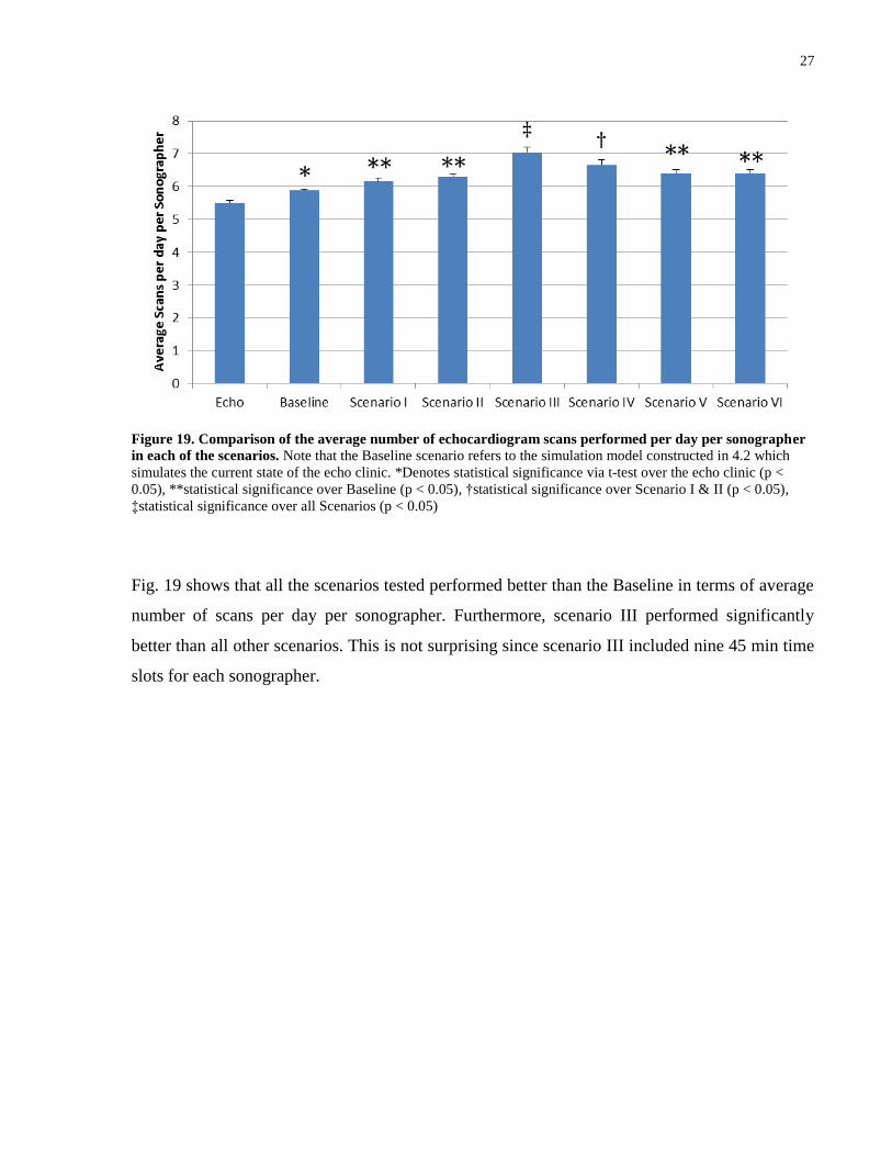
Figure 19. Comparison of the average number of echocardiogram scans performed per day per sonographer

in each of the scenarios. Note that the Baseline scenario refers to the simulation model constructed in 4.2 which

simulates the current state of the echo clinic. *Denotes statistical significance via t-test over the echo clinic (p <

0.05), **statistical significance over Baseline (p < 0.05), †statistical significance over Scenario I & II (p < 0.05),

‡statistical significance over all Scenarios (p < 0.05)

Fig. 19 shows that all the scenarios tested performed better than the Baseline in terms of average

number of scans per day per sonographer. Furthermore, scenario III performed significantly

better than all other scenarios. This is not surprising since scenario III included nine 45 min time

slots for each sonographer.

28

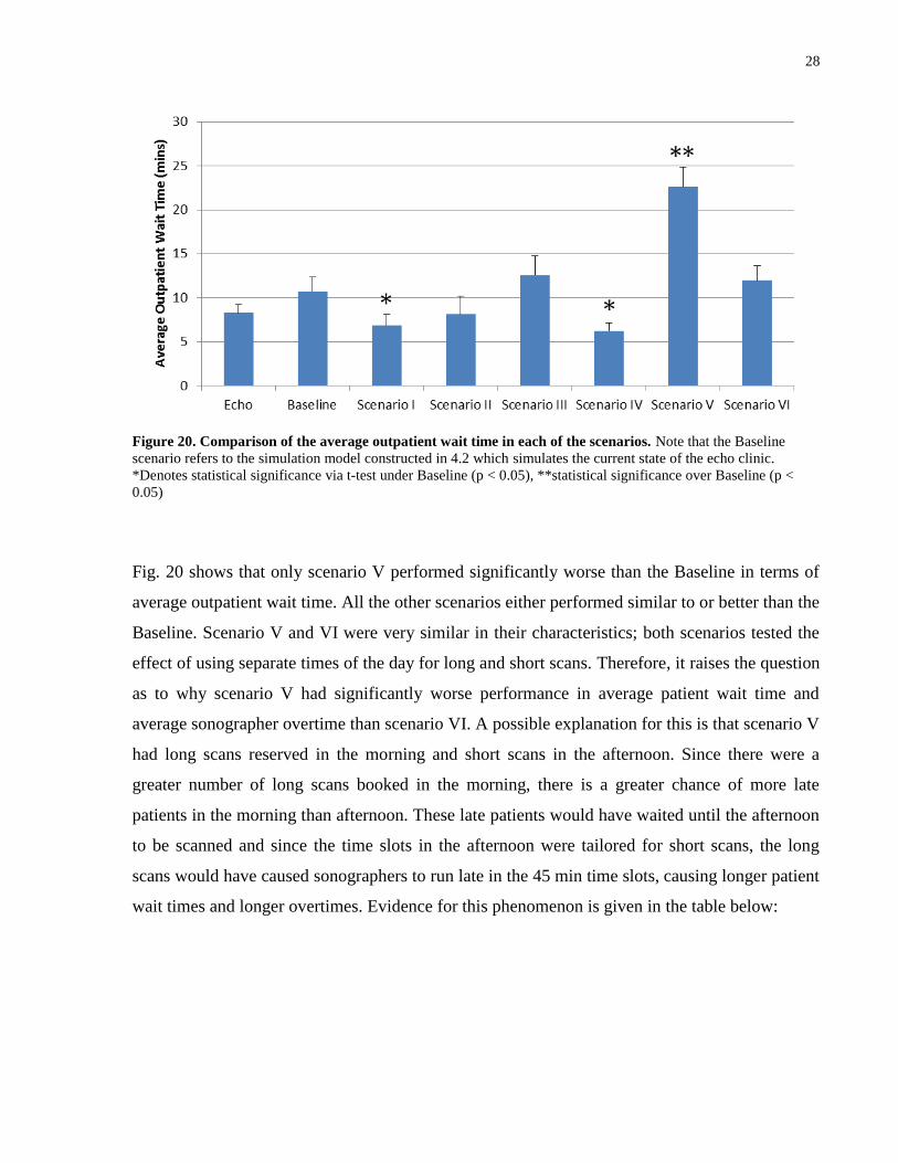
Figure 20. Comparison of the average outpatient wait time in each of the scenarios. Note that the Baseline

scenario refers to the simulation model constructed in 4.2 which simulates the current state of the echo clinic.

*Denotes statistical significance via t-test under Baseline (p < 0.05), **statistical significance over Baseline (p <

0.05)

Fig. 20 shows that only scenario V performed significantly worse than the Baseline in terms of

average outpatient wait time. All the other scenarios either performed similar to or better than the

Baseline. Scenario V and VI were very similar in their characteristics; both scenarios tested the

effect of using separate times of the day for long and short scans. Therefore, it raises the question

as to why scenario V had significantly worse performance in average patient wait time and

average sonographer overtime than scenario VI. A possible explanation for this is that scenario V

had long scans reserved in the morning and short scans in the afternoon. Since there were a

greater number of long scans booked in the morning, there is a greater chance of more late

patients in the morning than afternoon. These late patients would have waited until the afternoon

to be scanned and since the time slots in the afternoon were tailored for short scans, the long

scans would have caused sonographers to run late in the 45 min time slots, causing longer patient

wait times and longer overtimes. Evidence for this phenomenon is given in the table below:

29

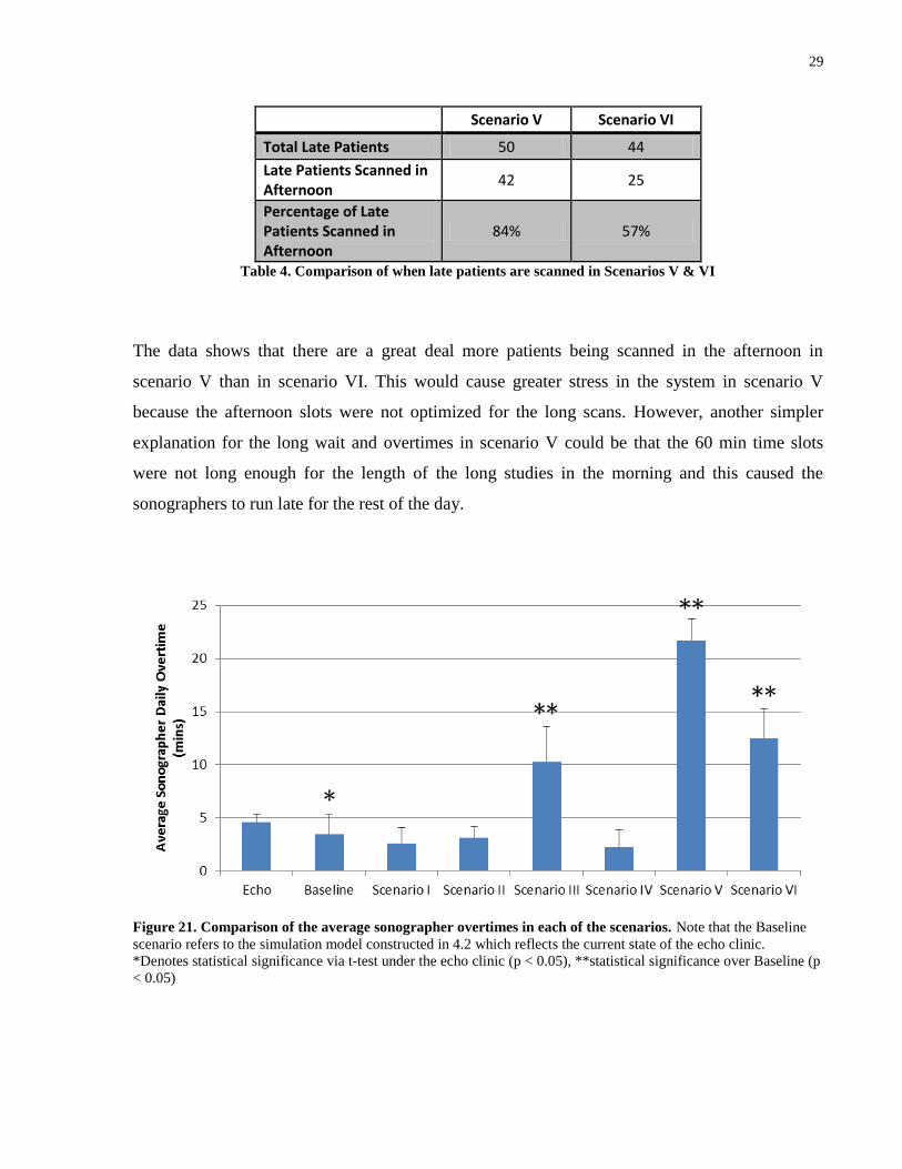
Scenario V Scenario VI

Total Late Patients 50 44

Late Patients Scanned in Afternoon

42 25

Percentage of Late Patients Scanned in Afternoon

84% 57%

Table 4. Comparison of when late patients are scanned in Scenarios V & VI

The data shows that there are a great deal more patients being scanned in the afternoon in

scenario V than in scenario VI. This would cause greater stress in the system in scenario V

because the afternoon slots were not optimized for the long scans. However, another simpler

explanation for the long wait and overtimes in scenario V could be that the 60 min time slots

were not long enough for the length of the long studies in the morning and this caused the

sonographers to run late for the rest of the day.

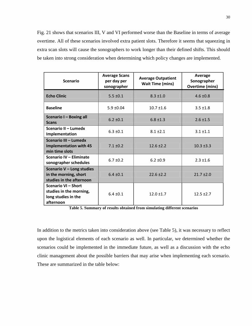
Figure 21. Comparison of the average sonographer overtimes in each of the scenarios. Note that the Baseline

scenario refers to the simulation model constructed in 4.2 which reflects the current state of the echo clinic.

*Denotes statistical significance via t-test under the echo clinic (p < 0.05), **statistical significance over Baseline (p

< 0.05)

30

Fig. 21 shows that scenarios III, V and VI performed worse than the Baseline in terms of average

overtime. All of these scenarios involved extra patient slots. Therefore it seems that squeezing in

extra scan slots will cause the sonographers to work longer than their defined shifts. This should

be taken into strong consideration when determining which policy changes are implemented.

Scenario Average Scans

per day per sonographer

Average Outpatient Wait Time (mins)

Average Sonographer

Overtime (mins)

Echo Clinic 5.5 ±0.1 8.3 ±1.0 4.6 ±0.8

Baseline 5.9 ±0.04 10.7 ±1.6 3.5 ±1.8

Scenario I – Boxing all Scans

6.2 ±0.1 6.8 ±1.3 2.6 ±1.5

Scenario II – Lumedx Implementation

6.3 ±0.1 8.1 ±2.1 3.1 ±1.1


7.1 ±0.2 12.6 ±2.2 10.3 ±3.3


6.7 ±0.2 6.2 ±0.9 2.3 ±1.6

Scenario V – Long studies in the morning, short studies in the afternoon

6.4 ±0.1 22.6 ±2.2 21.7 ±2.0


6.4 ±0.1 12.0 ±1.7 12.5 ±2.7

Table 5. Summary of results obtained from simulating different scenarios

In addition to the metrics taken into consideration above (see Table 5), it was necessary to reflect

upon the logistical elements of each scenario as well. In particular, we determined whether the

scenarios could be implemented in the immediate future, as well as a discussion with the echo

clinic management about the possible barriers that may arise when implementing each scenario.

These are summarized in the table below:

31

Scenario Can Implement Immediately?

Barriers to Implementation

Scenario I – Boxing all Scans Yes

-Will face resistance by cardiologists (and possibly sonographers) -Will need to immediately reschedule patients that need extra images

Scenario II – Lumedx Implementation

No -None


No -Will face resistance by sonographers -Need to start scheduling patients at 45 min intervals (could cause confusion)


Yes (No) -Need a way to track scan progress (so sonographers aren’t “hiding” in rooms)

Scenario V – Long studies in the morning, short studies in the afternoon Yes

-Resistance by sonographers -Need to start scheduling patients at 45 min intervals (could cause confusion) -Need to determine average lengths of all studies


Yes -Same as Scenario V

Table 6. Comparison of implementation feasibility of each of the scenarios

After taking all the metrics and logistical concerns into consideration, it was recommended that

scenario IV should be chosen to implement. In scenario IV, scan throughput increased by a

significant amount and patient wait times decreased by a significant amount. Furthermore,

average sonographer overtime did not significantly differ from the Baseline. It was also

determined that scenario IV could be implemented immediately. However it was recommended

that implementation of scenario IV occur after Lumedx is integrated into the system. Lumedx

integration would allow scan progress to be monitored, which would help to deter sonographers

from “hiding” in rooms. Lumdex would also help automate the task of assigning scans “on the

fly” and reduce cognitive load on the clerks.

32

6. CONCLUSION AND FUTURE WORK

The purpose of this project was to improve the current situation at an echocardiogram clinic at

the Hospital for Sick Children by increasing the number of scans per day. To achieve this goal,

the workflow of the echo clinic was assessed and a simulation model was constructed in order to

better understand the effects of various policy changes on performance measures, which include

number of scans per day, outpatient wait time, sonographer idle time, and sonographer overtime

Idle time was not observable, possibly due to the Hawthorne effect, and was subsequently

omitted as a metric. The results obtained from simulation model did not precisely reflect the

results obtained from the echo clinic, and this disparity was attributed to inherent limitations in

the simulation model. Nevertheless, the simulation model was still felt to have the ability to give

insight into how policy changes could affect the performance measures.

Six different policy change scenarios were explored. All scenarios yielded significant increases

in average scans per day per sonographer. Only scenario V performed significantly worse than

the Baseline in terms of average outpatient wait time. Scenarios III, V and VI performed worse

than Baseline in terms of average overtime. After considering logistical elements of each

scenario, such as time to implementation and possible barriers, Scenario IV was recommended

for implementation. In scenario IV, the average number of scans per day per sonographer

increased by a significant amount and the average patient wait time decreased by a significant

amount. The average sonographer overtime did not change significantly. The scenario is able to

be implemented immediately, but it was recommended that implementation should occur after

Lumedx is integrated into the echo clinic. Lumedx would give the clerks the ability to monitor

scan progress and will also help them assign scans to sonographers “on the fly”.

Future work for this project would involve obtaining in depth data for scan times. Specifically,

this will include obtaining scan time distributions for each type of echocardiogram study across

each sonographer working the clinic. This will allow the scheduler to more intelligently assign

scans to the sonographers. For example, sonographers could be primarily assigned to scan

studies that they are known to scan very quickly, and rarely assigned to scans that they are

known to scan slowly. Furthermore, obtaining specific scan time distributions for each

33

sonographer will improve the simulation model as the data can be used to eliminate the

homogeneity of the sonographers in simulation thereby making the simulation more of an

accurate reflection of the echo clinic.

34

7. REFERENCES

[1] N. Baily, "A study of queues and appointment systems in hospital outpatient departments

with special reference to waiting times," Journal of the Royal Statistical Society, vol. 14, p.

185–199, 1952.

[2] M. Blanco White and M. Pike, "Appointment systems in outpatients’ clinics and the effect

on patients’ unpunctuality," Medical Care, vol. 2, p. 133–145, 1964.

[3] T. Cayirli and E. Veral, "Outpatient scheduling in health care: A review of literature,"

Production and Operations Management, vol. 12, pp. 519-549, 2003.

[4] B. Fries and V. Marathe, "Determination of Optimal Variable-Sized Multiple-Block

Appointment Systems," Operations Research, vol. 29, pp. 324-345, 1981.

[5] C. Liao, C. Pegden and M. Rosenshine, "Planning Timely Arrivals to a Stochastic

Production or Service System," IIE Transactions, vol. 25, p. 63–73, 1993.

[6] L. Liu and X. Liu, "Dynamic and Static Job Allocation for Multi-Server Systems," IIE

Transactions, vol. 30, p. 845–854, 1998.

[7] K. Klassen and T. Rohleder, "Scheduling outpatient appointments in a dynamic

environment," Journal of Operations Management, vol. 14, pp. 83-101, 1996.

[8] E. Rising, R. Baron and B. Averill, "A System Analysis of a University Health Service

Outpatient Clinic," Operations Research, vol. 21, p. 1030–1047, 1973.

[9] T. Cox, J. Birchall and H. Wong, "Optimizing the Queuing System for an Ear, Nose and

Throat Outpatient Clinic," Journal of Applied Statistics, vol. 12, p. 113–126, 1985.

[10] J. Swisher, S. Jacobson, J. Jun and O. Balci, "Modeling and Analyzing a Physician Clinic

Environment Using Discrete-Event (Visual) Simulation," Computers & Operations

Research, vol. 28, pp. 105-125, 2001.

[11] R. O'Keefe, "Investigating Outpatient Departments: Implementable Policies and Qualitative

Approaches," Journal of the Operational Research Society, vol. 36, p. 705–712, 1985.

[12] E. Villegas, "Outpatient Appointment System Saves Time for Patients and Doctors,"

Hospitals, vol. 41, pp. 52-57, 1967.

[13] R. Fetter and J. Thompson, "Patients’ Waiting Time and Doctors’ Idle Time in the

Outpatient Setting," Health Services Research, vol. 1, pp. 66-90, 1966.

[14] M. Brahimi and D. Worthington, "The Finite Capacity Multi-Server Queue with

Inhomogeneous Arrival Rate and Discrete Service Time Distribution and Its Application to

Continuous Service Time Problems," European Journal of Operational Research, vol. 50,

p. 310–324, 1991.

[15] B. Lehaney, S. Clarke and J. Paul, "A Case of Intervention in an Outpatients Department,"

Journal of the Operational Research Society, vol. 50, p. 877–891, 1999.

[16] G. Swartzman, "The Patient Arrival Process in Hospitals: Statistical Analysis," Health

Services Research, vol. 5, p. 320–329, 1970.

[17] C. Ho and H. Lau, "Minimizing Total Cost in Scheduling Outpatient Appointments,"

Management Science, vol. 38, p. 1750–1764, 1992.

[18] R. Deyo and T. Inui, "Dropouts and Broken Appointments: A Literature Review and

Agenda for Future Research," Medical Care, vol. 18, p. 1146–1157, 1980.

35

[19] N. Weingarten, "Failed appointments in residency practices: Who misses them and what

providers are most affected?," Journal of the American Board of Family Practice, vol. 10,

pp. 407-411, 1997.

[20] W. Schafer, "Keep Patients Waiting? Not in My Office," Medical Economics, vol. 63, p.

137–141, 1986.

[21] T. Cayirli, E. Veral and H. Rosen, "Designing appointment scheduling systems for

ambulatory care services," Health Care Management Science, vol. 9, p. 47–58, 2006.

[22] T. Rohleder and K. Klassen, "Using Client-Variance Information to Improve Dynamic

Appointment Scheduling Performance," Omega, vol. 28, p. 293–302, 2000.

[23] H. Lau and A. Lau, "A Fast Procedure for Computing the Total System Cost of an

Appointment Schedule for Medical and Kindred Facilities," IIE Transactions, vol. 32, p.

833–839, 2000.

[24] P. Vanden Bosch and C. Dietz, "Minimizing Expected Waiting in a Medical Appointment

System," IIE Transactions, vol. 32, p. 841–848, 2000.

[25] W. Williams, R. Covert and J. Steele, "Simulation modeling of a teaching hospital

outpatient clinic.," Hospitals, vol. 41, pp. 71-75, 1967.

[26] M. Centeno, H. Dodd, M. Aranda and Y. Sanchez, "A simulation study to increase

throughput in an endoscopy center," Proceedings - Winter Simulation Conference, pp. 2462-

2473, 2010.

[27] S. Ramakrishnan, K. Nagarkar, M. DeGennaro, K. Srihari, A. Courtney and F. Emick, "A

study of the CT Scan area of a healthcare provider," Proceedings - Winter Simulation

Conference, vol. 2, pp. 2025-2031, 2004.

[28] J. Bennett and D. Worthington, "An example of a good but partially successful OR

engagement: Improving outpatient clinic operations," Interfaces, vol. 28, pp. 56-69, 1998.

[29] K. Leonard and M. Masatu, "Outpatient process quality evaluation and the Hawthorne

Effect," Social Science and Medicine, vol. 63, pp. 2330-2340, 2006.

36

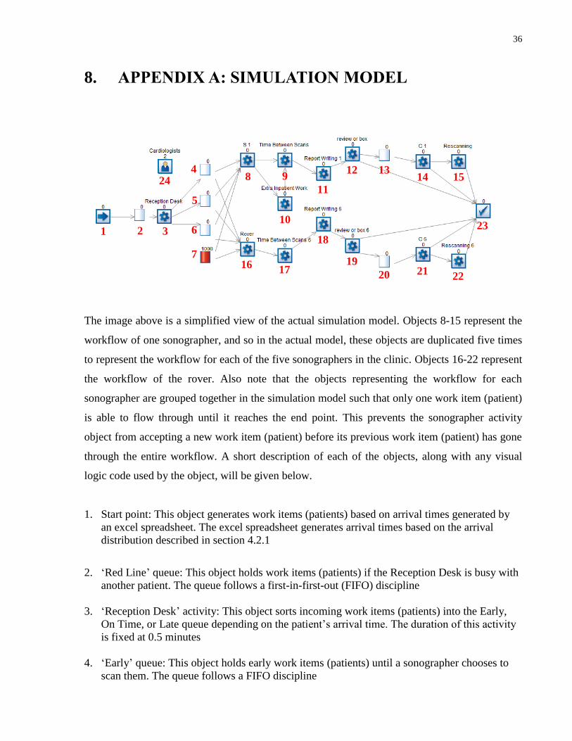
8. APPENDIX A: SIMULATION MODEL

The image above is a simplified view of the actual simulation model. Objects 8-15 represent the

workflow of one sonographer, and so in the actual model, these objects are duplicated five times

to represent the workflow for each of the five sonographers in the clinic. Objects 16-22 represent

the workflow of the rover. Also note that the objects representing the workflow for each

sonographer are grouped together in the simulation model such that only one work item (patient)

is able to flow through until it reaches the end point. This prevents the sonographer activity

object from accepting a new work item (patient) before its previous work item (patient) has gone

through the entire workflow. A short description of each of the objects, along with any visual

logic code used by the object, will be given below.

1. Start point: This object generates work items (patients) based on arrival times generated by

an excel spreadsheet. The excel spreadsheet generates arrival times based on the arrival

distribution described in section 4.2.1

2. ‘Red Line’ queue: This object holds work items (patients) if the Reception Desk is busy with

another patient. The queue follows a first-in-first-out (FIFO) discipline

3. ‘Reception Desk’ activity: This object sorts incoming work items (patients) into the Early,

On Time, or Late queue depending on the patient’s arrival time. The duration of this activity

is fixed at 0.5 minutes

4. ‘Early’ queue: This object holds early work items (patients) until a sonographer chooses to

scan them. The queue follows a FIFO discipline

4

7

8

6

5

9

10

11

12 13 14 15

23

16 17

18

19

20 21 22

24

1 2 3

37

5. ‘On Time’ queue: This object holds on time work items (patients) until a sonographer is

available to scan them. The queue follows a FIFO discipline

6. ‘Late’ queue: This object holds late work items (patients) until a sonographer chooses to scan

them. The queue follows a FIFO discipline

7. ‘Inpatient’ queue: This object holds inpatients until a sonographer chooses to scan them. The

queue has a start-up volume of 1000 work items to illustrate that there are always inpatients

ready to be scanned at any time during the simulation

8. ‘Sonographer scan’ activity: This object represents the image acquisition period. The

duration of this activity is given by the distribution described in section 4.2.1. Furthermore,

this object chooses which type of patient to scan and when to scan them depending on the

appointment rules described in section 4.1.1. It does this by executing the following visual

logic code just before a new work item (patient) is taken:

VL SECTION: S 1 Route In Before Logic

IF Simulation Time < 60

Set Route In Discipline S 1 , Locked

ELSE IF [Simulation Time >= 300] & [Simulation Time < 360] = 1


ELSE IF Simulation Time >= 540

IF [On Time.Count Contents > 0] | [Float.Count Contents > 0] | [Early.Count Contents

> 0] = 1

Set Route In Discipline S 1 , Priority

Set Route In Priority S 1 , On Time , 1

Set Route In Priority S 1 , Float , 2

Set Route In Priority S 1 , Early , 3

ELSE


ELSE IF On Time.Count Contents > 0

IF [Simulation Time > 60] & [Simulation Time < 90] = 1



ELSE IF [Simulation Time > 120] & [Simulation Time < 150] = 1












38







ELSE


ELSE

IF [Simulation Time > 65] & [Simulation Time < 90] = 1

IF Float.Count Contents > 0



ELSE IF Early.Count Contents > 0



ELSE IF Simulation Time < 90


Set Route In Priority S 1 , Inpatients , 1

ELSE












ELSE












ELSE




39









ELSE












ELSE












ELSE












ELSE


ELSE

40


The above code includes fudge factors in which sonographers will not take new outpatients

30 min before the start of their next appointment and will not take new inpatients 50 min

before the start of their next appointment (or end of their shift). Sonographers in the

simulation cannot make decisions and these fudge factors allowed the simulation model to

more accurately reflect the workings of the echo clinic.

The above code is for the three sonographers on the 8am-4pm shift. For the two sonographers

on the 8:30am-4:30pm shift, the code must be altered to account for the 30 min offset in

time. This is done by simply adding 30 to each if-statement that scrutinizes “Simulation

Time”. After this activity is finished, the work item (patient) will be routed to the ‘Time

between scans’ activity if it is an outpatient, or the ‘Extra inpatient work’ activity if it is an

inpatient

9. ‘Time between scans’ activity: This object represents the time between image acquisitions.

The duration of this activity is given by the distribution described in section 4.2.1

10. ‘Extra inpatient work’ activity: This object represents the extra time taken when

sonographers scan inpatients. It encompasses the time it takes to power up/down the

echocardiogram machine and move it to the inpatient room. The duration of this activity is

given an average of 10 minutes

11. ‘Report writing’ activity: This object represents the time taken to write the scan report once

the scan is completed. The duration of this activity is given by the distribution described in

section 4.2.1

12. ‘Review or box’ activity: This object determines whether a patient scan is to be reviewed by

the cardiologist or boxed. The object makes this decision based on the probability that 12%

of scans were boxed (see Fig. 12). If the scan is to be reviewed, then this object will route the

work item (patient) to the ‘Scan review wait’ queue. If the scan is to be boxed, then this

object will route the work item (patient) to the End point. The duration of this activity is

fixed at 0.5 minutes

13. ‘Scan review wait’ queue: This object holds work items (patients) until a cardiologist is

available for review.

14. ‘Cardiologist review’ activity: This object represents the time spent reviewing a scan. Work

items (patients) may only enter this activity if there is at least one available cardiologist

resource (see object 24). Otherwise the work item (patient) will have to remain in the ‘Scan

review wait’ queue until a cardiologist is free. The duration of this activity is given by the

distribution described in section 4.2.1. This object also determines whether or not a rescan is

necessary. It makes this decision based on the probability that 10% of scans required a rescan

(see Fig. 11). If the scan requires additional echocardiogram images, then this object will

route the work item (patient) to the ‘Rescanning’ activity. Otherwise, this object will route

the work item (patient) to the End point

41

15. ‘Rescanning’ activity: This object represents the time spent taking additional echocardiogram

images. The duration of this activity is given an average of 10 minutes

16. ‘Rover scan’ activity: This object represents the image acquisition period. The duration of

this activity is given by the distribution described in section 4.2.1. Furthermore, this object

chooses which type of patient to scan and when to scan them depending on the appointment

rules described in section 4.1.1. It does this by executing the following visual logic code just

before a new work item (patient) is taken:

VL SECTION: Rover Route In Before Logic

IF Simulation Time < 60

Set Route In Discipline Rover , Locked

ELSE IF [Simulation Time >= 300] & [Simulation Time < 360] = 1


ELSE IF Simulation Time >= 500


ELSE IF Inpatients.Count Contents > 0

Set Route In Discipline Rover , Priority

Set Route In Priority Rover , Inpatients , 1

17. ‘Time between scans for rover’ activity: This object represents the time between image

acquisitions for the rover. The duration of this activity is given by the distribution described

in section 4.2.1

18. See 11

19. See 12

20. See 13

21. See 14

22. See 15

23. End point: This object generates an excel data sheet with information about each work item’s

(patient) experience through the simulation. These include scheduled time of arrival, actual

time of arrival, wait time, and which sonographer performed their scan

24. ‘Cardiologists’ resource: This object allows us to set the amount of cardiologists available for

review, which is set at two

Documents

INCREASING THE DAILY THROUGHPUT OF ECHOCARDIOGRAM PATIENTS ... · ii Title: Increasing the Daily Throughput of Echocardiogram Patients using Discrete Event Simulation Degree: Master