Embed Size (px)
Citation preview

1
Increasing the Competitiveness of Manitoba’s Potato Industry
Investigators
Dr. Zachary Frederick (principle investigator 2017)
Dr. Oscar Molina and Garry Sloik (principle investigators 2016)
Dr. Alison Nelson- Agriculture and Agri-Food Canada (principle investigator 2015)
Dr. Mario Tenuta (Verticillium microsclerotia counts from soil 2016-17)
Dr. Francis Zvomuya (statistical consultation 2016-17)
Blair Geisel (data curation and statistical consultation 2016)
Rylee White, Charles Kuizon (student assistants 2016-17)
Research committee
Dan Sawatzky – Keystone Potato Producers Association (KPPA)
Bryce Regan – Simplot Canada II
Jason Coates - Simplot Canada II
Dan Parynuik – Simplot Canada II
Mary LeMere - McCain Foods
Craig Linde - Diversification Specialist (MAFRD)
Tim Hore - Manitoba Agriculture
Dr. Vikram Bisht - Manitoba Agriculture
Dr. Alison Nelson - Agriculture and Agri-Food Canada
Dr. Tracy Shinners-Carnelley – Peak of the Market
Andrew Ronald – KPPA Agronomist
Dave Buhler – Chipping Potato Grower Association of Manitoba
Russell Jonk - Seed Potato Growers Association of Manitoba
Dr. Zachary Frederick (Manitoba Horticultural Productivity Enhancement Centre Inc)
2
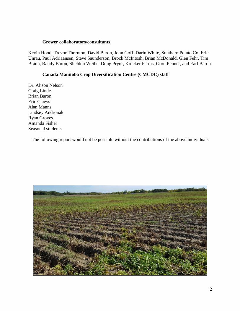
Grower collaborators/consultants
Kevin Hood, Trevor Thornton, David Baron, John Goff, Darin White, Southern Potato Co, Eric
Unrau, Paul Adriaansen, Steve Saunderson, Brock McIntosh, Brian McDonald, Glen Fehr, Tim
Braun, Randy Baron, Sheldon Weibe, Doug Pryor, Kroeker Farms, Gord Penner, and Earl Baron.
Canada Manitoba Crop Diversification Centre (CMCDC) staff
Dr. Alison Nelson
Craig Linde
Brian Baron
Eric Claeys
Alan Manns
Lindsey Andronak
Ryan Groves
Amanda Fisher
Seasonal students
The following report would not be possible without the contributions of the above individuals
3
Executive Summary
Increasing the Competitiveness of Manitoba’s Potato Industry
Manitoba potato growers must generate an increased yield of a high-quality crop grown in a
sustainable, cost effective manner to improve market competitiveness because of an upcoming
expansion in processing potential within Manitoba. Competitive factors outside our influence
include Manitoba’s distance to markets, global supply and demand of processed potato products,
and volatility in the exchange rate between Canada and the United States. Yield increases must
be achieved through regional research, development, and evaluation of crop management
strategies because the long-distance importation of research results from other areas risks
overlooking regionally significant yield-limiting factors. The overall goal of the research
program “Increasing the Competitiveness of Manitoba’s Potato Industry” is to foster sustainable,
competitive growth of the Manitoba potato industry through a research program within
Manitoba. The current objective of this research program was to identify areas of variable potato
yield and to characterize the variables responsible for variable yield. The future objective is to
compile the most important variables responsible for variable yield and evaluate strategies to
remediate each factor in-field.
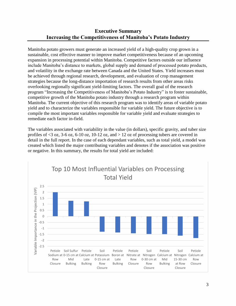
The variables associated with variability in the value (in dollars), specific gravity, and tuber size
profiles of <3 oz, 3-6 oz, 6-10 oz, 10-12 oz, and > 12 oz of processing tubers are covered in
detail in the full report. In the case of each dependant variables, such as total yield, a model was
created which listed the major contributing variables and denotes if the association was positive
or negative. In this summary, the results for total yield are included:
-2.5
-2
-1.5
-1
-0.5
0
0.5
1
1.5
2
2.5
PetioleSodium at
RowClosure
Soil Sulfur0-15 cm at
MidBulking
PetioleCalcium at
LateBulking
SoilPotassium0-15 cm at
RowClosure
PetioleBoron at
LateBulking
PetioleNitrate at
RowClosure
SoilNitrogen
0-30 cm atRow
Closure
PetioleCalcium at
MidBulking
SoilNitrogen15-30 cm
at RowClosure
PetioleCalcium at
RowClosure
Var
iab
le Im
po
rtan
ce in
th
e P
roje
ctio
n (
VIP
)
Top 10 Most Influential Variables on Processing Total Yield

4
Listed above are the top ten most influential positive and negative variables on total yield of
processing fields evaluated 2015-2017. The X axis (bottom) identifies the variable recorded,
whether it was from the soil or petioles, and the time of year it was collected. Nutrients were
generally recorded as lbs available to the plant in soil and PPM in petioles, as determined by
Agvise testing. The Y axis identifies the Variable of Importance in Projection (VIP) in the
creation of the model predicting total yield. Greater positive VIP (above zero) indicates that
variable has a bigger, positive association with yield. In other words, a bigger VIP indicates that
greater total yield from sampling points was associated with the increasing amount of this
nutrient in the soil or petiole. Lower, negative VIPs (below zero) indicates that variable has a
bigger negative association with yield. As the VIP drops, the increasing amount of that nutrient
is associated with the lowest yielding sampling points. The exact relationship between a negative
VIP and too much or too little of nutrient must be determined by a resource such as Agvise
recommendations or the Manitoba Soil Fertility guide
(https://www.gov.mb.ca/agriculture/crops/soil-fertility/soil-fertility-guide/). It is important to
note that 45-55 variables were associated with yield for all tuber size categories and total yield,
but only the top ten were reported here for simplicity.
The same type of models were created for each of the tuber size categories as total yield. It is
important to note that not all variables are consistent across total yield and each size category,
meaning that some variables are important for specific size categories. These variables can be the
target of remediation efforts if interest lies in improving the yield of that specific size category.
Variables that show up across some or all size categories are consistently associated with greater
or lesser potato yield, and the consistency is an important observation for remediation efforts to
improve yield regardless of size category. The figure below lists the top ten most influential
variables on 10-12 oz tubers to compare and contrast with total yield.

5
The most important variables contributing positively to both 10-12 oz tubers and total yield was
petiole sodium at row closure. Over the course of the experiment, the percentage sodium
recorded in the petiole by Agvise varied from 0.01% to 0.07%, indicating the percentage range
of positive benefit was small. However, the analysis indicated that the higher percentages were
associated with higher yielding sampling points. It is also important to note that the petiole
sodium content became a negative yield association from mid bulking and late bulking, albeit not
one of the top ten.
There were also two variables that were negatively associated with yield for both total yield and
10-12 oz yield. In these cases, too much or too little of either nutrient was associated with lower
yielding sampling points. A soil test and reference are necessary to determine whether it was too
much or too little – the model will not inform this result. Soil potassium at row closure from 0-15
cm was one such example, and 91 to 1150 PPM recorded as lowest to very high. The other
consistent variables were petiole calcium at row closure and mid bulking. The percentage of
petiole calcium at row closure ranged from 0.87-2.48%, which appeared to range from high to
very high. It is possible that excessive calcium was part of the negative yield association. Field
experimentation to address the relationship between calcium or potassium on negative yield
associations is absolutely necessary to verify this claim, especially before major management
decisions are implemented.
There are also many variables that appear on the top ten for total yield, but not 10-12 oz yield.
For example, sampling points with greater petiole nitrate at row closure are associated with total
yield negatively (i.e. greater petiole nitrate at row closure is associated with the lowest yielding
-2
-1.5
-1
-0.5
0
0.5
1
1.5
2
PetioleSodium at
RowClosure
PetioleCalcium at
MidBulking
PercentageSand 0-15
cm
SoilPotassium0-15 cm at
RowClosure
PetiolePotassium
at MidBulking
PetioleCalcium at
RowClosure
EC SoilReading 0-
15cm
PetiolePotassium
at LateBulking
PetioleCalcium at
LateBulking
Verticilliumdahliae
Propagules
Var
iab
le Im
po
rtan
ce in
a P
roje
ctio
n (
VIP
)Top 10 Most Influential Variables on Processing
Percentage 10-12 oz
6
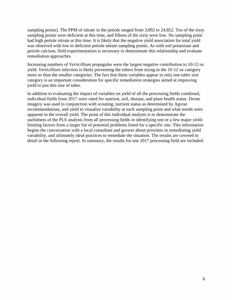
sampling points). The PPM of nitrate in the petiole ranged from 3,892 to 24,852. Ten of the sixty
sampling points were deficient at this time, and fifteen of the sixty were low. No sampling point
had high petiole nitrate at this time. It is likely that the negative yield association for total yield
was observed with low to deficient petiole nitrate sampling points. As with soil potassium and
petiole calcium, field experimentation is necessary to demonstrate this relationship and evaluate
remediation approaches.
Increasing numbers of Verticillium propagules were the largest negative contribution to 10-12 oz
yield. Verticillium infection is likely preventing the tubers from sizing in the 10-12 oz category
more so than the smaller categories. The fact that these variables appear in only one tuber size
category is an important consideration for specific remediation strategies aimed at improving
yield to just this size of tuber.
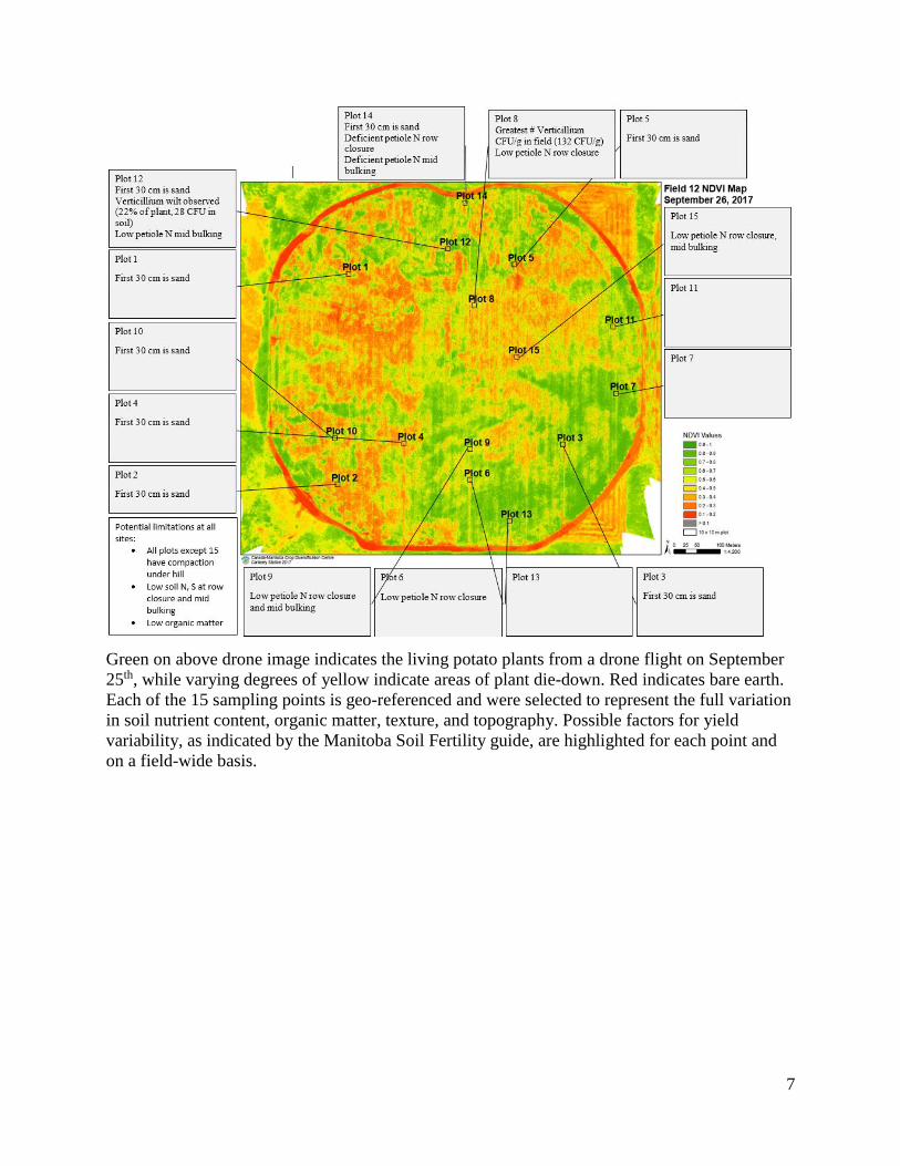
In addition to evaluating the impact of variables on yield of all the processing fields combined,
individual fields from 2017 were rated for nutrient, soil, disease, and plant health status. Drone
imagery was used in conjunction with scouting, nutrient status as determined by Agvise
recommendations, and yield to visualize variability at each sampling point and what trends were
apparent in the overall yield. The point of this individual analysis is to demonstrate the
usefulness of the PLS analysis from all processing fields in identifying one or a few major yield-
limiting factors from a larger list of potential problems listed for a specific site. This information
begins the conversation with a local consultant and grower about priorities in remediating yield
variability, and ultimately ideal practices to remediate the situation. The results are covered in
detail in the following report. In summary, the results for one 2017 processing field are included:
7
Green on above drone image indicates the living potato plants from a drone flight on September
25th, while varying degrees of yellow indicate areas of plant die-down. Red indicates bare earth.
Each of the 15 sampling points is geo-referenced and were selected to represent the full variation
in soil nutrient content, organic matter, texture, and topography. Possible factors for yield
variability, as indicated by the Manitoba Soil Fertility guide, are highlighted for each point and
on a field-wide basis.

8
The yield of the same field (#12), split by tuber size profile, is listed about by each sampling
point. Each point (1-15) on the above image corresponds to the plot numbers in the previous
image. Each color represents a specific tuber size profile. For example, yellow bars near the top
indicate the 10-11.9 oz tuber size. The yield is measured in hundredweight per acre (Cwt/A) on
the right side, and the harvest date was the first week in September. The green line connecting
the bars is the estimated dollar value of the sampling point. The scale for the dollar value is on
the left side.
In comparing the drone image of field 12 to the tuber size profile, some trends become apparent.
The lowest yielding sampling point number 14 was observed to have compaction under 30 cm,
low soil nitrogen and sulfur at row closure and mid bulking, low organic matter, high sand
composition, and deficient petiole nitrogen at row closure and mid bulking. It is possible that the
combination of some or all of these factors contributed to the yield limitation. This situation is
where the partial least squares regression (PLS) analysis from earlier can provide some clarity.
The sulfur concentration in the soil at mid bulking was an important, positive yield association
for total yield. The low soil sulfur at mid bulking could possibly be a large contributor to this
yield reduction. In addition, the noted low soil nitrogen availability is also an important variable
identified in the PLS regression analysis for all processing fields. Further trends are apparent as
the potential problems of an individual sampling point are cross-referenced with the PLS
regression analysis for each tuber size profile further into this report. The full set of conclusions
complete objective of this research program was to identify areas of variable potato yield and to
characterize the factors responsible for variable yield. These conclusions are expected to
influence the choices in meaningful yield variability remediation strategies and products are
evaluated moving forward in the future of this project.
Fields destined for processing were not the only market consideration throughout the course of
this project. Two fresh market fields were analyzed separately from processing fields in 2017.
The variables associated with variability in the misshapen tubers, knobs, growth cracks, enlarged
lenticels, russeting, and tuber size profiles of <2 in, 2-2.25 in, 2.25-3 in, 3-3.5 in, and > 3.5 in of
fresh market tubers is also covered in detail in the full report. In summary, only the results for
total yield are included:
0
100
200
300
400
500
600
0.000
1000.000
2000.000
3000.000
4000.000
5000.000
6000.000
7000.000
1 2 3 4 5 6 7 8 9 10 11 12 13 14 15
F12 Tuber Size Profile by Dollar Value
<3 oz 3-5.9 oz 6-9.9 oz
10-11.9 oz >12 oz dollars/cwt
9
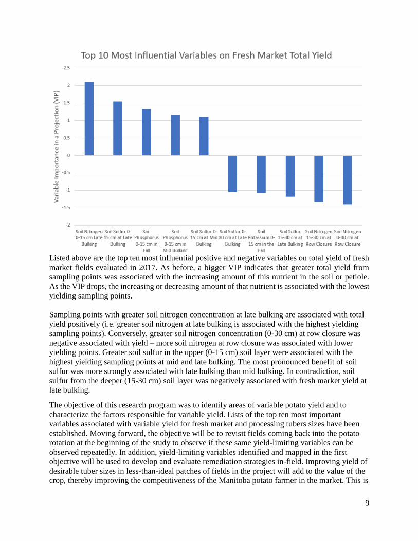
Listed above are the top ten most influential positive and negative variables on total yield of fresh
market fields evaluated in 2017. As before, a bigger VIP indicates that greater total yield from
sampling points was associated with the increasing amount of this nutrient in the soil or petiole.
As the VIP drops, the increasing or decreasing amount of that nutrient is associated with the lowest
yielding sampling points.
Sampling points with greater soil nitrogen concentration at late bulking are associated with total
yield positively (i.e. greater soil nitrogen at late bulking is associated with the highest yielding
sampling points). Conversely, greater soil nitrogen concentration (0-30 cm) at row closure was
negative associated with yield – more soil nitrogen at row closure was associated with lower
yielding points. Greater soil sulfur in the upper (0-15 cm) soil layer were associated with the
highest yielding sampling points at mid and late bulking. The most pronounced benefit of soil
sulfur was more strongly associated with late bulking than mid bulking. In contradiction, soil
sulfur from the deeper (15-30 cm) soil layer was negatively associated with fresh market yield at
late bulking.
The objective of this research program was to identify areas of variable potato yield and to
characterize the factors responsible for variable yield. Lists of the top ten most important
variables associated with variable yield for fresh market and processing tubers sizes have been
established. Moving forward, the objective will be to revisit fields coming back into the potato
rotation at the beginning of the study to observe if these same yield-limiting variables can be
observed repeatedly. In addition, yield-limiting variables identified and mapped in the first
objective will be used to develop and evaluate remediation strategies in-field. Improving yield of
desirable tuber sizes in less-than-ideal patches of fields in the project will add to the value of the
crop, thereby improving the competitiveness of the Manitoba potato farmer in the market. This is
10
important as processing expansions in Manitoba come into effect in the near future. Once
cooperators are satisfied by remediation strategies to variable yield, other Manitoba growers can
judge the fit of the practice to their operation. Remediation strategies that are adopted on a larger
scale provincially will amplify the desired goal to reach and improve the competitiveness of all
Manitoba potato growers.
Most studies examining one of the factors in the experiment, such as a nutrient, analyze said
factor in isolation as part of integrity the scientific method. While this regimented, narrowed
focus is imperative for results of ideal scientific integrity, the possibility exists that several
factors are inter-related. Strategies with the intent to mitigate one factor may require additional
adjustment to other areas to achieve the desired association observed in the results of this
document. Experience has taught the author that understand the complete range of interactions of
these 97 variables is very difficult for a singular individual entity to keep in mind, yet these
interactions remain important. The route to limiting this problem is the combined, group efforts
of the research committee, as well as growers and consultants. Only in working together can the
true objective of increasing the competitiveness of Manitoba’s potato industry be realized.
11
Introduction
Manitoba potato production has averaged 20.5 million hundredweight (cwt) annually from 2000
to 2013, landing the province with the #2 rank in Canadian potato production. Manitoba produces
20% of all the potatoes grown in Canada as of 2014 (Informa Economics, 2014). Manitoba has a
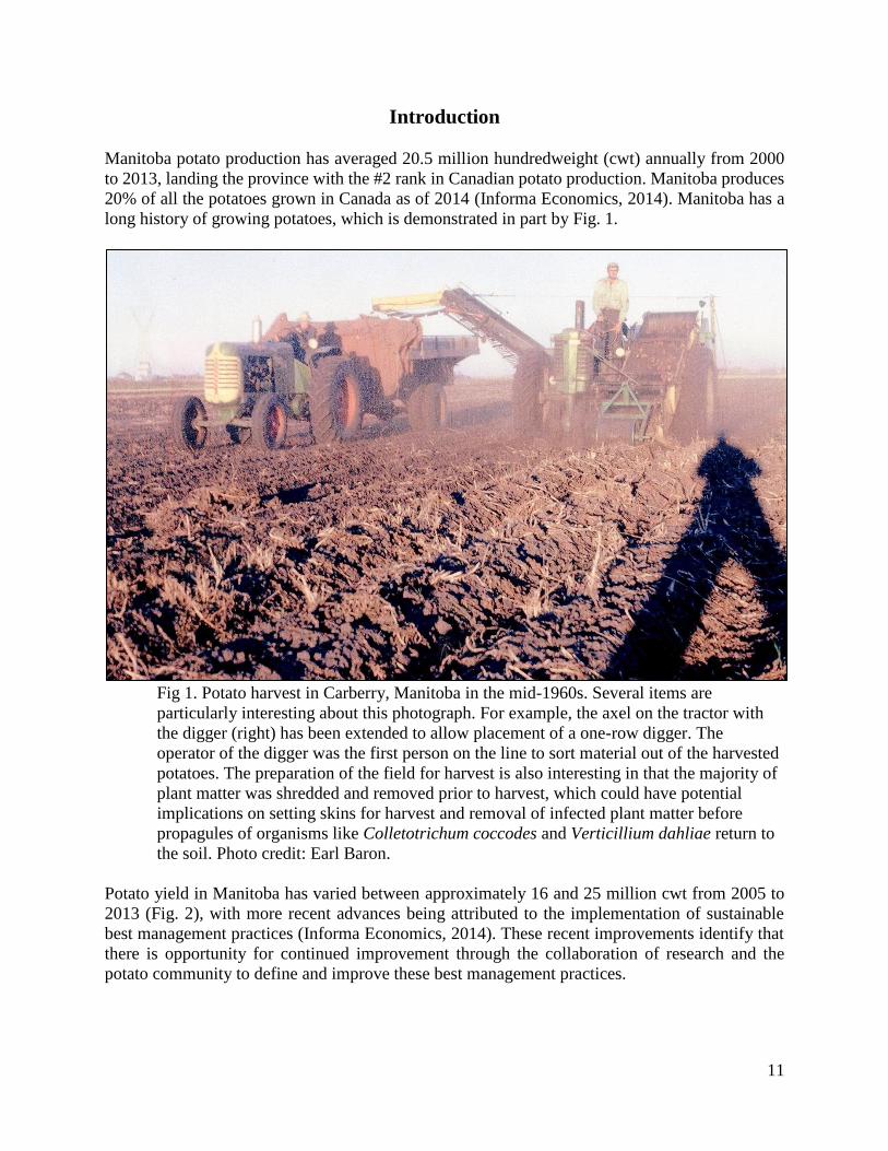
long history of growing potatoes, which is demonstrated in part by Fig. 1.
Fig 1. Potato harvest in Carberry, Manitoba in the mid-1960s. Several items are
particularly interesting about this photograph. For example, the axel on the tractor with
the digger (right) has been extended to allow placement of a one-row digger. The
operator of the digger was the first person on the line to sort material out of the harvested
potatoes. The preparation of the field for harvest is also interesting in that the majority of
plant matter was shredded and removed prior to harvest, which could have potential
implications on setting skins for harvest and removal of infected plant matter before
propagules of organisms like Colletotrichum coccodes and Verticillium dahliae return to
the soil. Photo credit: Earl Baron.
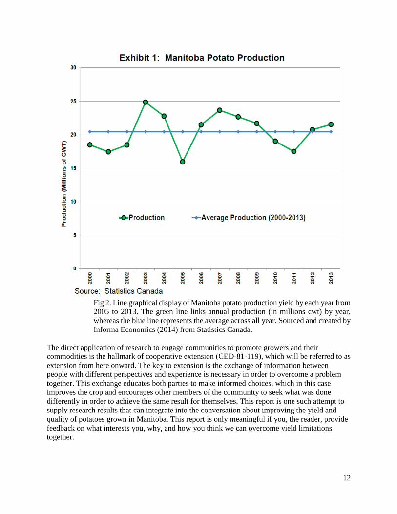
Potato yield in Manitoba has varied between approximately 16 and 25 million cwt from 2005 to
2013 (Fig. 2), with more recent advances being attributed to the implementation of sustainable
best management practices (Informa Economics, 2014). These recent improvements identify that
there is opportunity for continued improvement through the collaboration of research and the
potato community to define and improve these best management practices.
12
Fig 2. Line graphical display of Manitoba potato production yield by each year from
2005 to 2013. The green line links annual production (in millions cwt) by year,
whereas the blue line represents the average across all year. Sourced and created by
Informa Economics (2014) from Statistics Canada.
The direct application of research to engage communities to promote growers and their
commodities is the hallmark of cooperative extension (CED-81-119), which will be referred to as
extension from here onward. The key to extension is the exchange of information between
people with different perspectives and experience is necessary in order to overcome a problem
together. This exchange educates both parties to make informed choices, which in this case
improves the crop and encourages other members of the community to seek what was done
differently in order to achieve the same result for themselves. This report is one such attempt to
supply research results that can integrate into the conversation about improving the yield and
quality of potatoes grown in Manitoba. This report is only meaningful if you, the reader, provide
feedback on what interests you, why, and how you think we can overcome yield limitations
together.

13
The concept of cooperative extension is not new to North America– agricultural clubs and
societies of the early 19th century encouraged farmers to report their achievements on yield and
problem-solving. This practice of coming together to share knowledge to boost crop yield and
quality eventually led to events sponsored by local governments and universities the United
States, which eventually precipitated the formation of the land-grant college system in 1862
(CED-81-119). Attempts to overcome the current limitations of an agricultural system, potatoes
in this case, are inextricably intertwined with research and communal education efforts.
The Manitoba Crop Diversification Centre (MCDC) was established in 1993 with a ten-year
agreement amongst a community consisting of the Government of Canada, the Government of
Manitoba, and Manitoba Horticulture Productivity Enhancement Centre Inc. (MHPEC). Applied
research continues to this day under the name of the Canada-Manitoba Crop Diversification
Centre (CMCDC) on a five-year (2013-2018) agreement (Anonymous, 2017). Part of the
necessary information exchange for extension occurs at CMCDC through research in the areas of
crop diversification, intensive crop production technology practices, such as irrigation, and
facilitating development of value added processing of Manitoba-grown crops (Anonymous,
2016). Research reporting days, space for meetings for growers and industry, and individual
consultation with research agronomists means CMCDC is an integral part of the conversation to
exchange information to complete the purpose of extension for the Manitoba potato community.
The conversation to enhance Manitoba potato growers, as well as those involved in potato
processing and marketing, brings new challenges and opportunities for further research and
extension going into the future.
Manitoba potato growers must generate an increased yield of a high-quality crop grown in a
sustainable, cost effective manner to improve market competitiveness because of an upcoming
expansion in processing potential within Manitoba. Competitive factors outside our influence
include Manitoba’s distance to markets, global supply and demand of processed potato products,
and volatility in the exchange rate between Canada and the United States. Yield increases must
be achieved through regional research, development, and evaluation of crop management
strategies because the long-distance importation of research results from other areas risks
overlooking regionally significant yield-limiting factors. The overall goal of the research
program “Increasing the Competitiveness of Manitoba’s Potato Industry” is to foster sustainable,
competitive growth of the Manitoba potato industry through a research program within
Manitoba. This research program is conducted within grower fields, but is housed at CMCDC
and aligns with the centre’s objective of research into intensive crop production technology
practices.
The research program consisted of two objectives, and the first objective was to identify areas of
variable potato yield in specific fields and to characterize the factors responsible for variable
yield. A second objective uses yield-limiting factors identified in the previous objective to select
and evaluate strategies aimed at mitigating or compensating for these factors in field settings
specific to Manitoba.
This research program is designed to supply information on the remediation of yield limiting
factors for specific fields in Manitoba, which are generally representative of commercial
processing potato acres in Manitoba. The broader impact of this research is that remediation

14
strategies can be employed elsewhere in Manitoba to improve the yield or cost-effectiveness of
the potato crop. For example, the opposite of practices that are identified as selecting for larger
processing tubers could be considered by a seed grower for smaller seed potatoes. This goal can
only be achieved through the combined experience and research capacity of the Manitoba potato
growers, Manitoba Agriculture, Agriculture and Agri-Food Canada, the University of Manitoba,
the Keystone Potato Producers Association (KPPA), McCain Foods (Canada), Simplot Canada
II, the Chipping Potato Grower Association of Manitoba (CPGAM), and the Seed Potato
Growers Association of Manitoba (SPGAM).
Works Cited:
Anonymous. 2016. Canada-Manitoba Crop Diversification Centre Objectives. Published by the
Agriculture and Agri-Food Canada, retrieved from < http://www.agr.gc.ca/eng/about-us/offices-
and-locations/canada-manitoba-crop-diversification-centre/canada-manitoba-crop-
diversification-centre-objectives/?id=1185212178964? >
Anonymous. 2017. Canada-Manitoba Crop Diversification Centre. Published by the Agriculture
and Agri-Food Canada, retrieved from < http://www.agr.gc.ca/eng/about-us/offices-and-
locations/canada-manitoba-crop-diversification-centre/?id=1185205367529>
CED-81-119. 1981. Cooperative Extension Service's Mission and Federal Role Need
Congressional Clarification. United States General Accounting Office, Document Handling and
Information Services Facility. Retrieved from <https://www.gao.gov/products/CED-81-119>
Informa Economics. 2014. Manitoba Potato Industry Generates Over 1.4 Billion Dollars to the
Canadian Economy. Published by the Keystone Potato Producers Association, Chipping Potato
Growers of Manitoba, Seed Potato Growers of Manitoba, McCain Foods Canada, and Simplot
Canada II.
15
Results and Brief Discussion
Partial Least Squares regression analysis of all processing fields 2015-2017
(pooled data set)
Total Yield
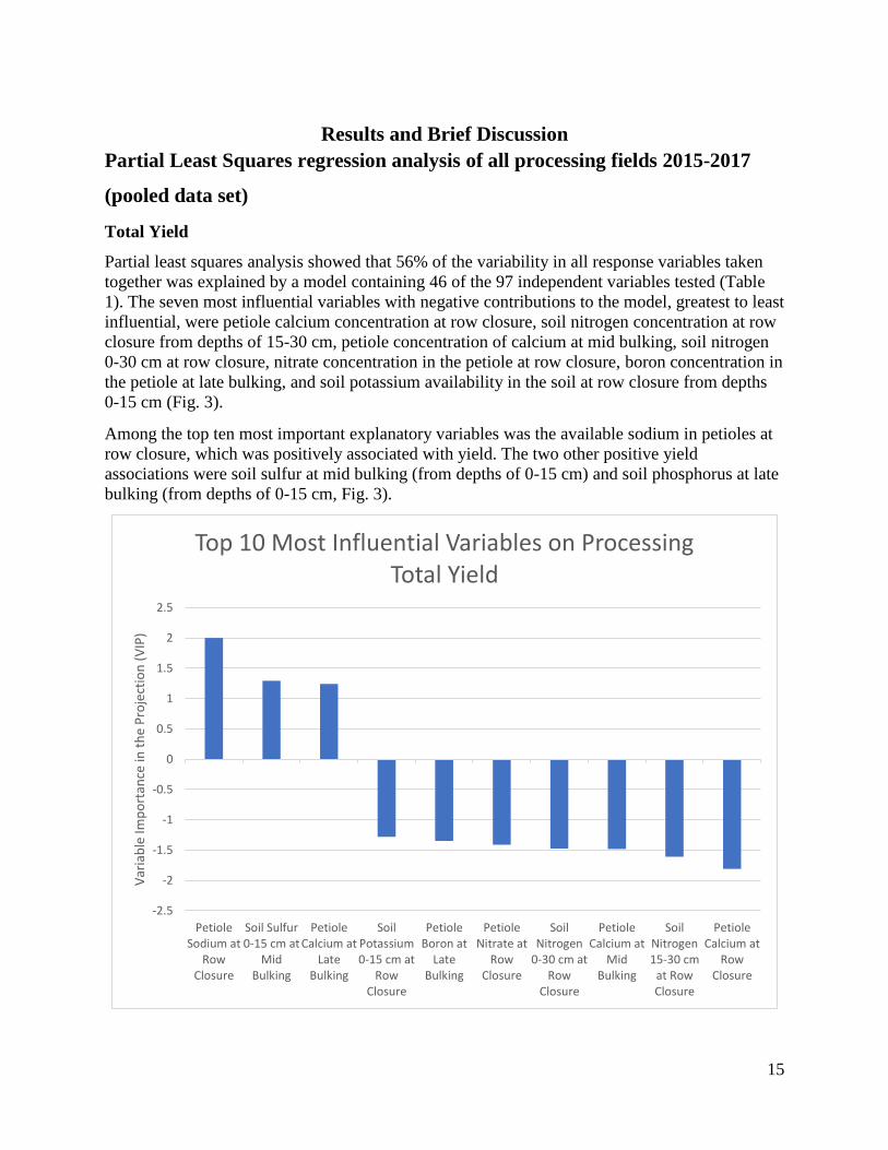
Partial least squares analysis showed that 56% of the variability in all response variables taken
together was explained by a model containing 46 of the 97 independent variables tested (Table
1). The seven most influential variables with negative contributions to the model, greatest to least
influential, were petiole calcium concentration at row closure, soil nitrogen concentration at row
closure from depths of 15-30 cm, petiole concentration of calcium at mid bulking, soil nitrogen
0-30 cm at row closure, nitrate concentration in the petiole at row closure, boron concentration in
the petiole at late bulking, and soil potassium availability in the soil at row closure from depths
0-15 cm (Fig. 3).
Among the top ten most important explanatory variables was the available sodium in petioles at
row closure, which was positively associated with yield. The two other positive yield
associations were soil sulfur at mid bulking (from depths of 0-15 cm) and soil phosphorus at late
bulking (from depths of 0-15 cm, Fig. 3).
-2.5
-2
-1.5
-1
-0.5
0
0.5
1
1.5
2
2.5
PetioleSodium at
RowClosure
Soil Sulfur0-15 cm at
MidBulking
PetioleCalcium at
LateBulking
SoilPotassium0-15 cm at
RowClosure
PetioleBoron at
LateBulking
PetioleNitrate at
RowClosure
SoilNitrogen
0-30 cm atRow
Closure
PetioleCalcium at
MidBulking
SoilNitrogen15-30 cm
at RowClosure
PetioleCalcium at
RowClosure
Var
iab
le Im
po
rtan
ce in
th
e P
roje
ctio
n (
VIP
)
Top 10 Most Influential Variables on Processing Total Yield
16
Fig. 3. Listed above are the top ten most influential positive and negative variables on total yield
of processing fields evaluated 2015-2017. The X axis (bottom) identifies the variable recorded,
whether it was from the soil or petioles, and the time of year it was collected. Nutrients were
generally recorded as lbs available to the plant in soil and PPM in petioles, as determined by
Agvise testing. The Y axis identifies the Variable of Importance in Projection (VIP) in the
creation of the model predicting total yield. Greater positive VIP (above zero) indicates that
variable has a bigger, positive association with yield. In other words, a bigger VIP indicates that
greater total yield from sampling points was associated with the increasing amount of this
nutrient in the soil or petiole. Lower, negative VIPs (below zero) indicates that variable has a
bigger negative association with yield. As the VIP drops, the increasing or decreasing amount of
that nutrient is associated with the lowest yielding sampling points. The exact relationship
between a negative VIP and too much or too little of nutrient must be determined by a resource
such as Agvise recommendations or the Manitoba Soil Fertility guide
(https://www.gov.mb.ca/agriculture/crops/soil-fertility/soil-fertility-guide/). It is important to
note that 45-55 variables were associated with yield for all tuber size categories and total yield,
but only the top ten were reported here for simplicity.
The interpretation of these results is that variables with greater VIPs have greater significance to
the model (Table 1), and therefore have greater variance between the sampling points with
greater and lesser total yield. For example, sampling points with greater petiole nitrogen at row
closure are associated with total yield negatively and could be translated as less petiole nitrate at
row closure is associated with our lowest yielding sampling points. Over the course of the
experiment, petiole nitrate results varied from 3892 to 32668. The association with decreasing
total yield would focus on the upper range of 32668, but the exact cut off of when the benefit of
available nitrogen turns to detriment cannot be determined by this form of analysis.
Recommendations from Agvise suggest that the cut off is around 25000, but experimental
validation with a remediation strategy (objective 2) aimed at identifying nitrogen practices prior
to row closure and their effect on the ideal petiole range are needed before experimentally-
validated recommendations can be issued.
Variables such as available sodium in the petiole are positively associated with total yield,
indicating the best-yielding sampling points were associated with more petiole sodium than the
lower yielding points. Over the course of the experiment, the percentage sodium recorded in the
petiole by Agvise varied from 0.01% to 0.07%, indicating the percentage range of positive
benefit was small. However, the analysis indicated that the higher percentages were associated
with higher yielding sampling points. It is also important to note that the petiole sodium content
became a negative yield association from mid bulking and late bulking, albeit not one of the top
ten.
Similarly, increased sulfur concentration in the upper (0-15 cm) horizon of the soil at mid
bulking was associated with our highest yielding sampling points. However, the benefit to total
yield associated with greater petiole sodium is larger than the benefit from increased soil sulfur,
as indicated by an increased VIP in the model (i.e. the higher the bar is on the positive side, the
greater the benefit, and the lower the bar on the negative side indicates incrementally larger
negative effect).
The results on petiole calcium are also interesting in that sampling points with greater petiole
calcium had lower total yield. In this case, too much or too little of calcium was associated with

17
lower yielding sampling points. A soil test and reference are necessary to determine whether it
was too much or too little – the model will not inform this result. The percentage of petiole
calcium at row closure ranged from 0.87-2.48%, which appeared to range from high to very
high. It is possible that excessive calcium was part of the negative yield association. Field
experimentation to address the relationship with calcium on negative yield associations is
absolutely necessary to verify this claim, especially before major management decisions are
implemented.
It is very to get lost in the morass of results and interpretation of the following results for each
size category. Repetition is key to the integrity of any result from any scientific study. The
conclusions section will list the consistent results across all size categories and total yield for the
processing and fresh sections of this report.
Value of the crop in dollars
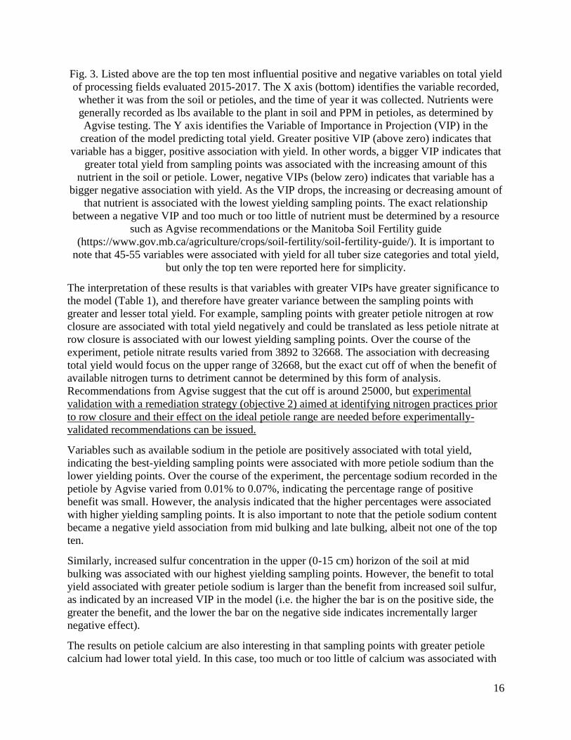
When the total dollar value of the crop was tested individually, a two-component model
containing 46 variables explained 58% of the variability was generated with strong predictive
power (Table 2). The seven most influential variables with negative contributions to the model,
greatest to least influential, were calcium concentration in the petiole at row closure, nitrogen
concentration in the 15-30 cm soil layer at row closure, soil nitrogen concentration from 0-30 cm
at row closure, calcium concentration in the petiole at mid bulking, sulfur concentration in the
15-30 cm soil layer at row closure, calcium concentration in the petiole at late bulking, and
sodium concentration in the petiole at late bulking (Fig. 4).
The three most influential variables with a significant, positive contributions to the model,
greatest to least influential, were the sodium concentration in the petiole at row closure, soil
nitrogen 0-15 cm at row closure, and soil potassium 0-15 cm at row closure (Fig. 4).
18
Fig. 4. The top 10 most influential positive and negative variables on the value of processing
fields evaluated 2015-2017. The X axis (bottom) identifies the variable recorded, whether it was
from the soil or petioles, and the time of year it was collected. Nutrients were generally recorded
as lbs available to the plant in soil as determined by Agvise testing and nutrient
recommendations. The Y axis identifies the Variable of Importance in Projection (VIP) in the
creation of the model for this yield category. Greater positive VIP (above zero) indicates that
variable has a bigger positive association with yield. Lesser negative VIP (below zero) indicates
that variable has a bigger negative association with yield.
The interpretation of these results is that variables with greater VIPs have greater significance to
the model (Table 2), and therefore have greater variance between the sampling points with
greater and lesser value in dollars. More valuable sampling points were associated with higher
petiole sodium at row closure than less valuable sampling points. More valuable sampling points
were associated with lower calcium concentrations in the petiole at row closure or lower nitrogen
concentration in the 0-15 cm soil layer at row closure than less valuable sampling points, for
example. The negative association with petiole calcium at row closure was greater than soil
nitrogen at row closure (VIP greater for petiole calcium).
The pounds of nitrogen available in the soil varied at row closure from 5 to 160 lbs, which can
explain the anomalous result that increasing soil nitrogen can be a positive value association, but
too much or too little is a negative value association. Five pounds of available soil nitrogen is too
little by row closure – limiting growth and eventual bulking, and ultimately reducing value. The
-2.5
-2
-1.5
-1
-0.5
0
0.5
1
1.5
2
2.5
PetioleSodium at
RowClosure
SoilNitrogen
0-15 cm atRow
Closure
SoilPotassium0-15 cm at
RowClosure
PetioleSodium at
LateBulking
PetioleCalcium at
LateBulking
Soil Sulfur0-15 cm at
MidBulking
PetioleCalcium at
MidBulking
SoilNitrogen
0-30 cm atRow
Closure
SoilNitrogen15-30 cm
at RowClosure
PetioleCalcium at
RowClosure
Var
iab
le Im
po
rtan
ce in
th
e P
roje
ctio
n (
VIP
)Top 10 Most Influential Variables on Processing
Value
19
consultants that took part in the 2017 year of the project seem to aim for 130-180 lbs of nitrogen
in the soil by row closure, which includes the upper range of 160 lbs nitrogen in the soil
observed in the experiment. This could explain the result where increasing soil nitrogen (up to
the 160 lbs max observed) at the 0-15 cm is a positive yield association. However, too much or
too little decrease value. Field experimentation is necessary to place the association in the
context of an actual on-farm practice.
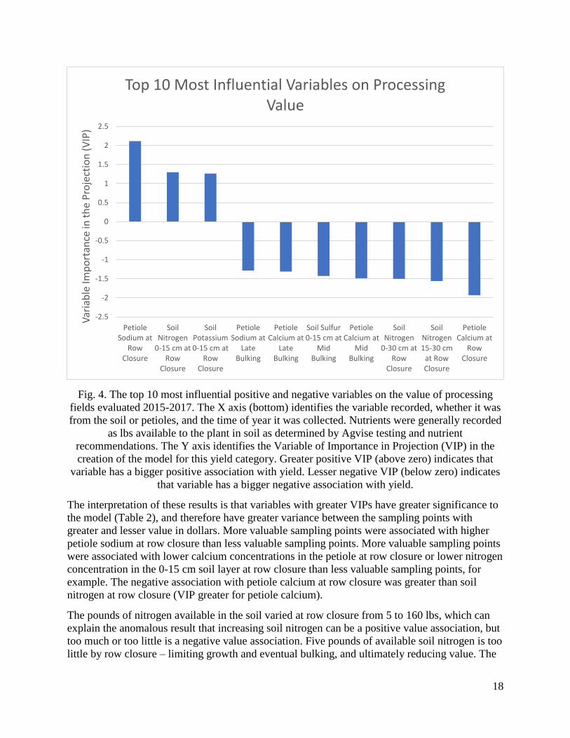
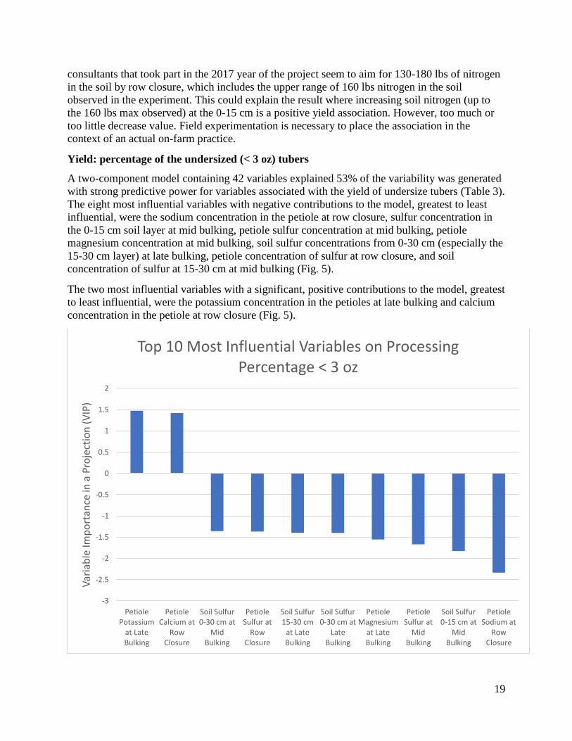
Yield: percentage of the undersized (< 3 oz) tubers
A two-component model containing 42 variables explained 53% of the variability was generated
with strong predictive power for variables associated with the yield of undersize tubers (Table 3).
The eight most influential variables with negative contributions to the model, greatest to least
influential, were the sodium concentration in the petiole at row closure, sulfur concentration in
the 0-15 cm soil layer at mid bulking, petiole sulfur concentration at mid bulking, petiole
magnesium concentration at mid bulking, soil sulfur concentrations from 0-30 cm (especially the
15-30 cm layer) at late bulking, petiole concentration of sulfur at row closure, and soil
concentration of sulfur at 15-30 cm at mid bulking (Fig. 5).
The two most influential variables with a significant, positive contributions to the model, greatest
to least influential, were the potassium concentration in the petioles at late bulking and calcium
concentration in the petiole at row closure (Fig. 5).
-3
-2.5
-2
-1.5
-1
-0.5
0
0.5
1
1.5
2
PetiolePotassium
at LateBulking
PetioleCalcium at
RowClosure
Soil Sulfur0-30 cm at
MidBulking
PetioleSulfur at
RowClosure
Soil Sulfur15-30 cm
at LateBulking
Soil Sulfur0-30 cm at
LateBulking
PetioleMagnesium
at LateBulking
PetioleSulfur at
MidBulking
Soil Sulfur0-15 cm at
MidBulking
PetioleSodium at
RowClosure
Var
iab
le Im
po
rtan
ce in
a P
roje
ctio
n (
VIP
)
Top 10 Most Influential Variables on Processing Percentage < 3 oz
20
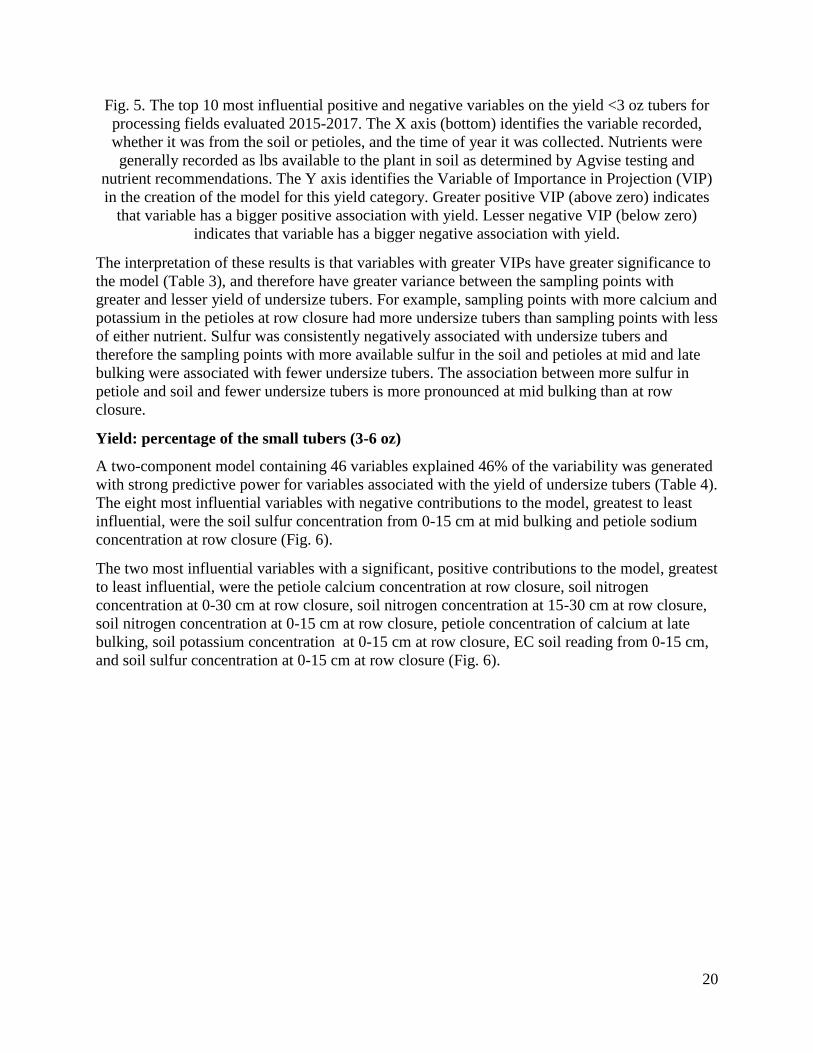
Fig. 5. The top 10 most influential positive and negative variables on the yield <3 oz tubers for
processing fields evaluated 2015-2017. The X axis (bottom) identifies the variable recorded,
whether it was from the soil or petioles, and the time of year it was collected. Nutrients were
generally recorded as lbs available to the plant in soil as determined by Agvise testing and
nutrient recommendations. The Y axis identifies the Variable of Importance in Projection (VIP)
in the creation of the model for this yield category. Greater positive VIP (above zero) indicates
that variable has a bigger positive association with yield. Lesser negative VIP (below zero)
indicates that variable has a bigger negative association with yield.
The interpretation of these results is that variables with greater VIPs have greater significance to
the model (Table 3), and therefore have greater variance between the sampling points with
greater and lesser yield of undersize tubers. For example, sampling points with more calcium and
potassium in the petioles at row closure had more undersize tubers than sampling points with less
of either nutrient. Sulfur was consistently negatively associated with undersize tubers and
therefore the sampling points with more available sulfur in the soil and petioles at mid and late
bulking were associated with fewer undersize tubers. The association between more sulfur in
petiole and soil and fewer undersize tubers is more pronounced at mid bulking than at row
closure.
Yield: percentage of the small tubers (3-6 oz)
A two-component model containing 46 variables explained 46% of the variability was generated
with strong predictive power for variables associated with the yield of undersize tubers (Table 4).
The eight most influential variables with negative contributions to the model, greatest to least
influential, were the soil sulfur concentration from 0-15 cm at mid bulking and petiole sodium
concentration at row closure (Fig. 6).
The two most influential variables with a significant, positive contributions to the model, greatest
to least influential, were the petiole calcium concentration at row closure, soil nitrogen
concentration at 0-30 cm at row closure, soil nitrogen concentration at 15-30 cm at row closure,
soil nitrogen concentration at 0-15 cm at row closure, petiole concentration of calcium at late
bulking, soil potassium concentration at 0-15 cm at row closure, EC soil reading from 0-15 cm,
and soil sulfur concentration at 0-15 cm at row closure (Fig. 6).
21
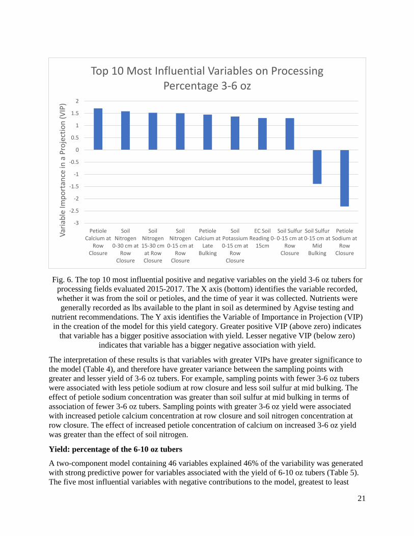
Fig. 6. The top 10 most influential positive and negative variables on the yield 3-6 oz tubers for
processing fields evaluated 2015-2017. The X axis (bottom) identifies the variable recorded,
whether it was from the soil or petioles, and the time of year it was collected. Nutrients were
generally recorded as lbs available to the plant in soil as determined by Agvise testing and
nutrient recommendations. The Y axis identifies the Variable of Importance in Projection (VIP)
in the creation of the model for this yield category. Greater positive VIP (above zero) indicates
that variable has a bigger positive association with yield. Lesser negative VIP (below zero)
indicates that variable has a bigger negative association with yield.
The interpretation of these results is that variables with greater VIPs have greater significance to
the model (Table 4), and therefore have greater variance between the sampling points with
greater and lesser yield of 3-6 oz tubers. For example, sampling points with fewer 3-6 oz tubers
were associated with less petiole sodium at row closure and less soil sulfur at mid bulking. The
effect of petiole sodium concentration was greater than soil sulfur at mid bulking in terms of
association of fewer 3-6 oz tubers. Sampling points with greater 3-6 oz yield were associated
with increased petiole calcium concentration at row closure and soil nitrogen concentration at
row closure. The effect of increased petiole concentration of calcium on increased 3-6 oz yield
was greater than the effect of soil nitrogen.
Yield: percentage of the 6-10 oz tubers
A two-component model containing 46 variables explained 46% of the variability was generated
with strong predictive power for variables associated with the yield of 6-10 oz tubers (Table 5).
The five most influential variables with negative contributions to the model, greatest to least
-3
-2.5
-2
-1.5
-1
-0.5
0
0.5
1
1.5
2
PetioleCalcium at
RowClosure
SoilNitrogen
0-30 cm atRow
Closure
SoilNitrogen15-30 cm
at RowClosure
SoilNitrogen
0-15 cm atRow
Closure
PetioleCalcium at
LateBulking
SoilPotassium0-15 cm at
RowClosure
EC SoilReading 0-
15cm
Soil Sulfur0-15 cm at
RowClosure
Soil Sulfur0-15 cm at
MidBulking
PetioleSodium at
RowClosure
Var
iab
le Im
po
rtan
ce in
a P
roje
ctio
n (
VIP
)Top 10 Most Influential Variables on Processing
Percentage 3-6 oz
22
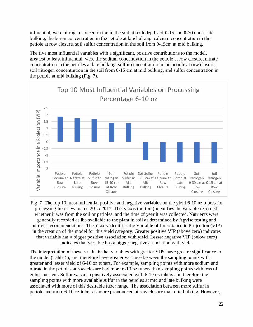
influential, were nitrogen concentration in the soil at both depths of 0-15 and 0-30 cm at late
bulking, the boron concentration in the petiole at late bulking, calcium concentration in the
petiole at row closure, soil sulfur concentration in the soil from 0-15cm at mid bulking.
The five most influential variables with a significant, positive contributions to the model,
greatest to least influential, were the sodium concentration in the petiole at row closure, nitrate
concentration in the petioles at late bulking, sulfur concentration in the petiole at row closure,
soil nitrogen concentration in the soil from 0-15 cm at mid bulking, and sulfur concentration in
the petiole at mid bulking (Fig. 7).
Fig. 7. The top 10 most influential positive and negative variables on the yield 6-10 oz tubers for
processing fields evaluated 2015-2017. The X axis (bottom) identifies the variable recorded,
whether it was from the soil or petioles, and the time of year it was collected. Nutrients were
generally recorded as lbs available to the plant in soil as determined by Agvise testing and
nutrient recommendations. The Y axis identifies the Variable of Importance in Projection (VIP)
in the creation of the model for this yield category. Greater positive VIP (above zero) indicates
that variable has a bigger positive association with yield. Lesser negative VIP (below zero)
indicates that variable has a bigger negative association with yield.
The interpretation of these results is that variables with greater VIPs have greater significance to
the model (Table 5), and therefore have greater variance between the sampling points with
greater and lesser yield of 6-10 oz tubers. For example, sampling points with more sodium and
nitrate in the petioles at row closure had more 6-10 oz tubers than sampling points with less of
either nutrient. Sulfur was also positively associated with 6-10 oz tubers and therefore the
sampling points with more available sulfur in the petioles at mid and late bulking were
associated with more of this desirable tuber range. The association between more sulfur in
petiole and more 6-10 oz tubers is more pronounced at row closure than mid bulking. However,
-2
-1.5
-1
-0.5
0
0.5
1
1.5
2
2.5
PetioleSodium at
RowClosure
PetioleNitrate at
LateBulking
PetioleSulfur at
RowClosure
SoilNitrogen15-30 cm
at RowClosure
PetioleSulfur at
MidBulking
Soil Sulfur0-15 cm at
MidBulking
PetioleCalcium at
RowClosure
PetioleBoron at
LateBulking
SoilNitrogen
0-30 cm atRow
Closure
SoilNitrogen
0-15 cm atRow
ClosureVar
iab
le Im
po
rtan
ce in
a P
roje
ctio
n (
VIP
)
Top 10 Most Influential Variables on Processing Percentage 6-10 oz

23
sampling points with more petiole boron and soil nitrogen at late bulking were associated with
fewer 6-10 oz tubers.
Yield: percentage of the 10-12 oz tubers
A two-component model containing 50 variables explained 52% of the variability was generated
with strong predictive power for variables associated with the yield of 10-12 oz tubers (Table 6).
The nine most influential variables with negative contributions to the model, greatest to least
influential, were the number of Verticillium dahliae propagules (as evaluated by the PCR test),
calcium concentration in the petioles at late bulking, potassium concentration in the petiole at
late bulking, EC soil reading from 0-15cm, calcium concentration in the petiole at row closure,
petiole potassium concentration at row closure, soil potassium concentration from 0-15 cm at
row closure, percentage sand 0-15 cm, and the calcium concentration in the petiole at mid
bulking (Fig. 8).
The only influential variable (of the top 10 total) with a significant, positive contribution to the
model was the petiole sodium concentration by row closure (Fig. 8).
Fig. 8. The top 10 most influential positive and negative variables on the yield 10-12 oz tubers
for processing fields evaluated 2015-2017. The X axis (bottom) identifies the variable recorded,
whether it was from the soil or petioles, and the time of year it was collected. Nutrients were
generally recorded as lbs available to the plant in soil as determined by Agvise testing and
nutrient recommendations. The Y axis identifies the Variable of Importance in Projection (VIP)
-2
-1.5
-1
-0.5
0
0.5
1
1.5
2
PetioleSodium at
RowClosure
PetioleCalcium at
Mid Bulking
PercentageSand 0-15
cm
SoilPotassium0-15 cm at
RowClosure
PetiolePotassium
at MidBulking
PetioleCalcium at
RowClosure
EC SoilReading 0-
15cm
PetiolePotassium
at LateBulking
PetioleCalcium at
LateBulking
Verticilliumdahliae
Propagules
Var
iab
le Im
po
rtan
ce in
a P
roje
ctio
n (
VIP
)
Top 10 Most Influential Variables on Processing Percentage 10-12 oz
24
in the creation of the model for this yield category. Greater positive VIP (above zero) indicates
that variable has a bigger positive association with yield. Lesser negative VIP (below zero)
indicates that variable has a bigger negative association with yield.
The interpretation of these results is that variables with greater VIPs have greater significance to
the model (Table 6), and therefore have greater variance between the sampling points with
greater and lesser yield of 10-12 oz tubers. There was only one variable observed, sodium
concentration in the petiole at row closure, where sampling points with more 10-12 oz tubers had
more sodium than sampling points with lower 10-12 oz yield. Over the course of the experiment,
the percentage sodium recorded in the petiole by Agvise varied from 0.01% to 0.07%, indicating
the percentage range of positive benefit was small. However, the analysis indicated that the
higher percentages were associated with higher yielding sampling points. It is also important to
note that the petiole sodium content became a negative yield association from mid bulking and
late bulking, albeit not one of the top ten.
Interestingly, sampling points with more Verticillium propagules had fewer 10-12 oz tubers. This
is the only observation in the whole experiment where Verticillium was a variable of greater
significance than most of the nutrients tested on impacting the yield of a specific tuber size
profile. In the case of Verticillium, greater numbers of propagules per gram of soil were
associated with the sampling points with the lowest percentages of 10-12 oz tubers. It is
generally accepted that 5 to 30 CFUs per gram of soil are necessary to infect a potato plant
(Colony Forming Units – a form of propagule observed under a microscope while growing on a
petri plate). In the case of the experiment, CFU counts in excess of 100 in sampling points is
where 10-12 oz yield begins to drop. More discussion on Verticillium counts in specific fields
can be found in the “2017 Processing Field Individual Analysis” section.
The results on petiole calcium are also interesting in that sampling points with greater petiole
calcium had fewer 10-12 oz tubers at any of the sampling dates, but our earliest sampling at row
closure had the most pronounced effect of the three sampling dates. The final result to note is
that more available sulfur in the petioles and soil at mid and late bulking improved 6-10 oz yield,
but more soil sulfur at mid bulking decreased 10-12 oz yield. In these cases, too much or too
little of either nutrient was associated with lower yielding sampling points. A soil test and
reference are necessary to determine whether it was too much or too little – the model will not
inform this result. Soil potassium at row closure from 0-15 cm was one such example, and 91 to
1150 PPM recorded as lowest to very high. The other consistent variables were petiole calcium
at row closure and mid bulking. The percentage of petiole calcium at row closure ranged from
0.87-2.48%, which appeared to range from high to very high. It is possible that excessive
calcium was part of the negative yield association. Field experimentation to address the
relationship between calcium or potassium on negative yield associations is absolutely necessary
to verify this claim, especially before major management decisions are implemented.
Yield: percentage of the 6-12 oz combined tuber size categories
A two-component model containing 44 variables explained 57% of the variability was generated
with strong predictive power for variables associated with the yield of 6-12 oz tubers (Table 7).
The seven most influential variables with negative contributions to the model, greatest to least
influential, were the calcium concentration in the petiole at row closure, nitrogen concentration
in the soil at both depths of 0-15 and 0-30 cm, boron concentration in the petiole at late bulking,
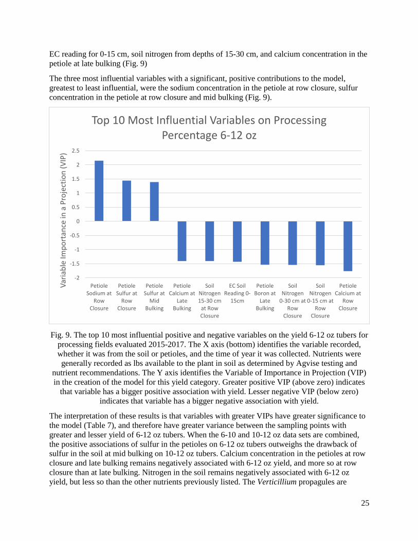
25
EC reading for 0-15 cm, soil nitrogen from depths of 15-30 cm, and calcium concentration in the
petiole at late bulking (Fig. 9)
The three most influential variables with a significant, positive contributions to the model,
greatest to least influential, were the sodium concentration in the petiole at row closure, sulfur
concentration in the petiole at row closure and mid bulking (Fig. 9).
Fig. 9. The top 10 most influential positive and negative variables on the yield 6-12 oz tubers for
processing fields evaluated 2015-2017. The X axis (bottom) identifies the variable recorded,
whether it was from the soil or petioles, and the time of year it was collected. Nutrients were
generally recorded as lbs available to the plant in soil as determined by Agvise testing and
nutrient recommendations. The Y axis identifies the Variable of Importance in Projection (VIP)
in the creation of the model for this yield category. Greater positive VIP (above zero) indicates
that variable has a bigger positive association with yield. Lesser negative VIP (below zero)
indicates that variable has a bigger negative association with yield.
The interpretation of these results is that variables with greater VIPs have greater significance to
the model (Table 7), and therefore have greater variance between the sampling points with
greater and lesser yield of 6-12 oz tubers. When the 6-10 and 10-12 oz data sets are combined,
the positive associations of sulfur in the petioles on 6-12 oz tubers outweighs the drawback of
sulfur in the soil at mid bulking on 10-12 oz tubers. Calcium concentration in the petioles at row
closure and late bulking remains negatively associated with 6-12 oz yield, and more so at row
closure than at late bulking. Nitrogen in the soil remains negatively associated with 6-12 oz
yield, but less so than the other nutrients previously listed. The Verticillium propagules are
-2
-1.5
-1
-0.5
0
0.5
1
1.5
2
2.5
PetioleSodium at
RowClosure
PetioleSulfur at
RowClosure
PetioleSulfur at
MidBulking
PetioleCalcium at
LateBulking
SoilNitrogen15-30 cm
at RowClosure
EC SoilReading 0-
15cm
PetioleBoron at
LateBulking
SoilNitrogen
0-30 cm atRow
Closure
SoilNitrogen
0-15 cm atRow
Closure
PetioleCalcium at
RowClosure
Var
iab
le Im
po
rtan
ce in
a P
roje
ctio
n (
VIP
)
Top 10 Most Influential Variables on Processing Percentage 6-12 oz

26
notably absent from the top 10 list of negative associations of 6-12 oz tubers, meaning
Verticillium still negatively impacts yield, but the nutrients listed previously are more deleterious
to yield than Verticillium in the fields we have sampled at this time. It is important to note that,
as a biological system, areas where Verticillium dahliae infections become a prominent potato
problem tend to grow in size and increase in severity with time, necessitating long-term
management strategies even if it currently isn’t the most important yield limiting factor.
Yield: percentage of the > 12 oz tubers
A two-component model containing 43 variables explained 48% of the variability was generated
with strong predictive power for variables associated with the yield of >12 oz tubers (Table 8).
The seven most influential variables with negative contributions to the model, greatest to least
influential, were the soil nitrogen availability at row closure for both depths of 0-15 and 15-30
cm, organic matter at depths of 0-15 cm, percentage of soil silt 0-15 cm, soil sulfur concentration
at mid bulking, and gravimetric water content 0-12 cm (Fig. 10).
The three most influential variables with a significant, positive contributions to the model,
greatest to least influential, were the sodium concentration in the petiole at row closure, sulfur
concentration in the soil from depths of 0-15 and 0-30 cm at row closure (Fig. 10).
Fig. 10. The top 10 most influential positive and negative variables on the yield > 12 oz tubers
for processing fields evaluated 2015-2017. The X axis (bottom) identifies the variable recorded,
whether it was from the soil or petioles, and the time of year it was collected. Nutrients were
generally recorded as lbs available to the plant in soil as determined by Agvise testing and
nutrient recommendations. The Y axis identifies the Variable of Importance in Projection (VIP)
-2
-1.5
-1
-0.5
0
0.5
1
1.5
2
2.5
3
PetioleSodium at
RowClosure
Soil Sulfur0-15 cm at
RowClosure
Soil Sulfur0-30 cm at
RowClosure
GravimetricWater
Content 0-12 cm
Soil Sulfur0-15 cm at
Mid Bulking
PercentageSilt 15-30
cm
Soil OrganicMatter 0-15
cm
SoilNitrogen 0-
15 cm atRow
Closure
SoilNitrogen
15-30 cm atRow
Closure
SoilNitrogen 0-
30 cm atRow
Closure
Var
iab
le Im
po
rtan
ce in
a P
roje
ctio
n (
VIP
)
Top 10 Most Influential Variables on Processing Percentage > 12 oz
27
in the creation of the model for this yield category. Greater positive VIP (above zero) indicates
that variable has a bigger positive association with yield. Lesser negative VIP (below zero)
indicates that variable has a bigger negative association with yield.
The interpretation of these results is that variables with greater VIPs have greater significance to
the model (Table 9), and therefore have greater variance between the sampling points with
greater and lesser yield of > 12 oz tubers. Increased soil nitrogen at row closure, regardless of
depth, is associated with decreased yield of tubers > 12 oz and 6-10 oz. This stands in contrast to
increased soil nitrogen at row closure associating with more >3 oz tubers. The > 12 oz size
category is unique in that organic matter, silt percentage, and moisture content are in the top ten
most influential variables that are negatively associated with yield. The positive association of
soil sulfur at row closure with >12 oz yield aligns with the general positive yield associations
with sulfur on 6-10 oz and 6-12 oz tubers.
Tuber specific gravity
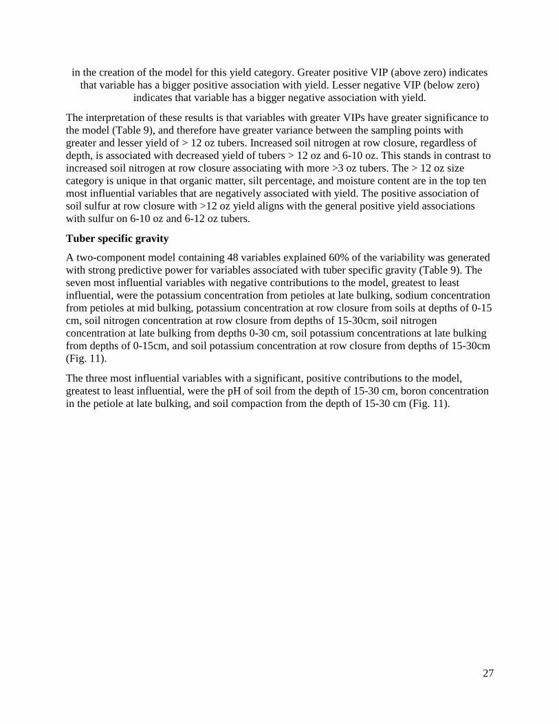
A two-component model containing 48 variables explained 60% of the variability was generated
with strong predictive power for variables associated with tuber specific gravity (Table 9). The
seven most influential variables with negative contributions to the model, greatest to least
influential, were the potassium concentration from petioles at late bulking, sodium concentration
from petioles at mid bulking, potassium concentration at row closure from soils at depths of 0-15
cm, soil nitrogen concentration at row closure from depths of 15-30cm, soil nitrogen
concentration at late bulking from depths 0-30 cm, soil potassium concentrations at late bulking
from depths of 0-15cm, and soil potassium concentration at row closure from depths of 15-30cm
(Fig. 11).
The three most influential variables with a significant, positive contributions to the model,
greatest to least influential, were the pH of soil from the depth of 15-30 cm, boron concentration
in the petiole at late bulking, and soil compaction from the depth of 15-30 cm (Fig. 11).
28
Fig. 11. The top 10 most influential positive and negative variables on specific gravity of
processing tubers evaluated 2015-2017. The X axis (bottom) identifies the variable recorded,
whether it was from the soil or petioles, and the time of year it was collected. Nutrients were
generally recorded as lbs available to the plant in soil as determined by Agvise testing and
nutrient recommendations. The Y axis identifies the Variable of Importance in Projection (VIP)
in the creation of the model for this yield category. Greater positive VIP (above zero) indicates
that variable has a bigger positive association with yield. Lesser negative VIP (below zero)
indicates that variable has a bigger negative association with yield.
The interpretation of these results is that variables with greater VIPs have greater significance to
the model (Table 10), and therefore have greater variance between the sampling points with
greater and lesser specific gravity of tubers. Boron concentration of the petiole was higher in
sampling points with higher specific gravity at late bulking. Petiole boron varied from 22 to 39
PPM over the course of the experiment, although this analysis doesn’t exactly identify the
relationship at which too much petiole boron pushes for too high of a specific gravity.
Tuber specific gravity was otherwise observed as increasing as soil compaction and pH increased
at depths of 15-30 cm.
Too much or too little soil potassium and nitrogen was associated with decreased specific
gravity. The soil nitrogen values have been identified previously, but the late bulking soil
potassium values varied from 87 to 1032 lbs. It is possible that both too much and too little soil
potassium could present problems, but further field experimentation is necessary to link exact
soil potassium values with specific gravity variability.
-2
-1.5
-1
-0.5
0
0.5
1
1.5
2
Soil pH 15-30 cm
PetioleBoron Late
Bulking
SoilCompaction
0-30 cm
SoilPotassium0-15 cm at
LateBulking
SoilNitrogen 0-
30 cm atLate
Bulking
SoilNitrogen 0-
15 cm atRow
Closure
SoilNitrogen
15-30 cm atLate
Bulking
SoilPotassium0-15 cm at
RowClosure
PetioleSodium at
Mid Bulking
PetiolePotassium
at LateBulking
Var
iab
le Im
po
rtan
ce in
a P
roje
ctio
n (
VIP
)Top 10 Most Influential Variables on Specific Gravity of
Processing Tubers
29
Drone Image Analysis
Drone images from 2017 processing fields had the NDVI values (scale 0-1 vegetative index)
were extracted and pooled for all processing fields for regression analysis independent of the
partial least squares regression discussed previously. This data was analyzed separately because
there was only data for only one year, which doesn’t represent the entire project. The limitation
of this analysis is that factors outside of those listed could influence the result, but could not be
part of the analysis. More years of data are necessary to solidify the following results, and results
that interest the committee merit the creation of their own, independent experiment to fully
validate results before recommendations can be issued.
In summary, only significant results will be presented.
• Drone flights taken in June were positively associated with total yield (i.e. the greener
spots identified by the drone correlated well with the highest yielding points (P =
0.0031).
• Drone flights taken in June (P = 0.0051) and August 18-21 (P = 0.0265) were negatively
associated with 3-6 oz yield. Drone images at these dates could become part of a
predictive tool using the drone to associate certain parts of the field with less 3-6 oz
tubers.
• Drone flights taken in June were positively associated with 6-12 oz yield (i.e. the greener
spots identified by the drone correlated well with the highest yielding points (P =
0.0467).
The June flight results are interesting when combined with individual field analysis drone images
to follow in that there is a possibility of using the June flight as a predictive tool for problem
places in certain fields.
30
2017 Processing Field Individual Analysis
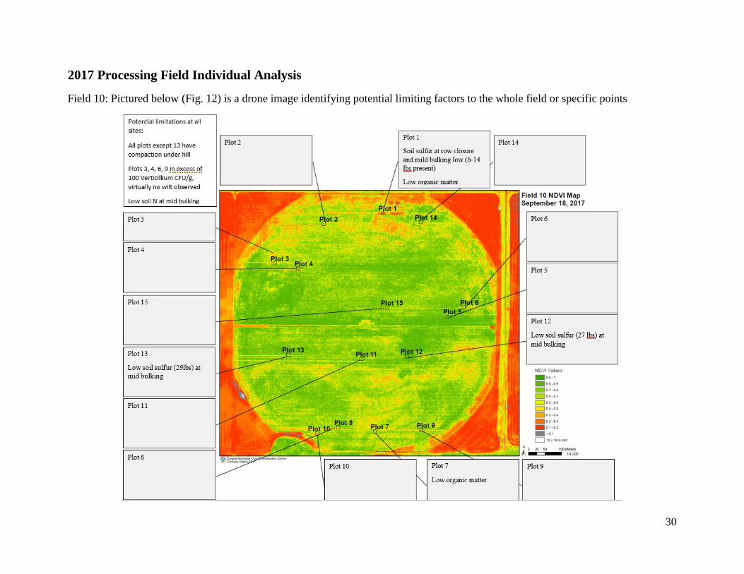
Field 10: Pictured below (Fig. 12) is a drone image identifying potential limiting factors to the whole field or specific points
31
In addition to evaluating the impact of variables on yield of fresh and processing fields together, individual fields from 2017 were
rated for nutrient, soil, disease, and plant health status. Drone imagery was used in conjunction with scouting, nutrient status as
determined by Agvise recommendations, and yield to visualize variability at each sampling point and what trends were apparent in the
overall yield. The point of this individual analysis is to demonstrate the usefulness of the Partial Least Square (PLS) analysis from all
processing fields in identifying one or a few major yield-limiting factors from a larger list of potential problems listed for a specific
site. This information begins the conversation with a local consultant and grower about priorities in remediating yield variability, and
ultimately develop practices to remediate the situation.
Plot numbers in the drone images refer to the 15 sampling points in each field. The top of each image is north in each field, and the
color scale refers to the NDVI values recorded by the drone. NDVI was recorded on a scale of 0-1, zero being red and refers to bare
earth, 1 refers to green tissue, and varying shades of green to yellow indicate senescencing plant matter. It is important to note that
weed canopy color will be recorded as well as potato, although no significant weed pressure was recorded in the sampling points in
field 10.
For each individual field, certain variables were identified as potential problems for the whole field or individual collection points that
could contribute to variable yield. Field 10 was observed to have compaction under the hill (beneath 30 cm/11.8 in from top of hill)
with an excess of 300 PSI. The only sampling point that was not compacted at this layer was plot 13, on the southwestern side of the
field. Compaction was not among the top ten most influential variables listed in the complete processing analysis, indicating that it
could be a problem on an individual field basis, but not among the worse problems across all processing fields.
Very little Verticillium wilt was recorded in the field, but Verticillium species counts exceeded 100 CFU /g in plots 3, 4, 6, and 9. It is
generally accepted that 5-30 CFU/g of V. dahliae are necessary for infection. This plate count will encompass all Verticillium species,
which doesn’t accurately rely the number of V. dahliae CFU. Verticillium will likely need to be monitored in the field, but the disease
is unlikely to be the cause of variable yield observed this year. The combined processing analysis indicated that the 10-12oz yield
category is the size range most negatively impacted by high Vertcillium counts, as severely infected plants are killed or debilitated
during late bulking when tubers are sizing in this range. Concern about any drops in 10-12 oz yield should consider the Verticillium
counts in future years based on this information.
The main indicators of variable yield, among the variables recorded for the study, in this field are low soil nitrogen and sulfur at mid
bulking. Low soil nitrogen was recorded across all collection points at mid bulking, whereas low soil sulfur was a more sporadic
problem with no obvious trend. Both sulfur and nitrogen were important nutrients involved in variable yield across all processing
fields, with low soil sulfur at mid bulking and soil nitrogen at row closure being associated with lower yielding sampling points.
32
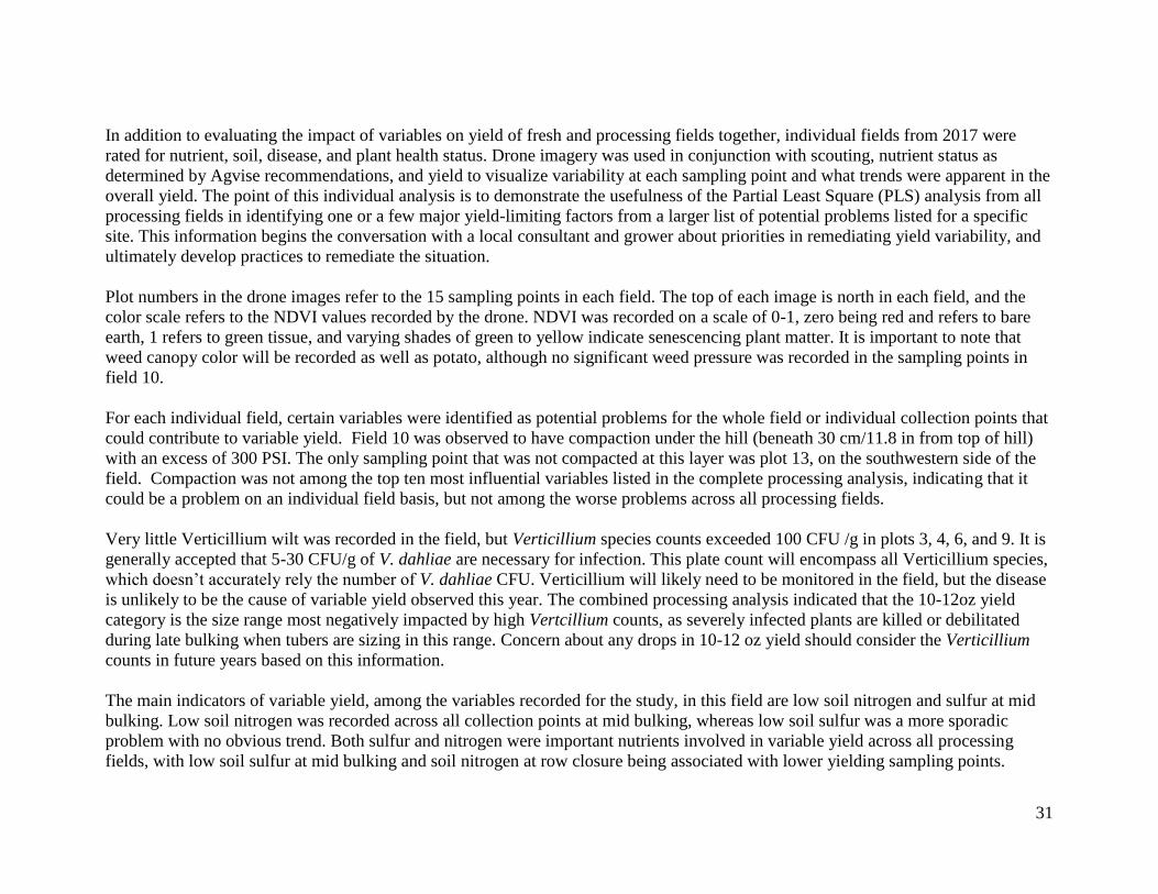
Throughout the study, the lowest yielding points often had multiple potential limiting factors listed in the drone image like Fig. 12.
Some of these limiting factors are inter-related, such as sand texture and nitrogen leaching. In the case of field 10, only point one had
four potential factors. It is extremely likely that the combined effects of multiple problems contribute to yield limitation greater when
combined than each factor individually.
Fig 13. (Above) is another method of viewing the drone image from three drone flights at once. Each line represents an individual
flight, and each flight date is on the bottom. The 1-15 on the bottom (X-axis) refers to each of the 15 sampling points. The scale on the
Y-axis on the left refers to the same 0-1 NDVI scale as in Fig. 13 where zero is a dead plant and one is a perfectly green plant. The
flights selected only show the beginning and end of the season. The scale is lower in June as some places have yet to close, and by
July (not shown) the scale is at one across all points. As the line moves across the collection points, some trends in the greener (higher
NDVI) points are apparent as opposed to the browner (lower NDVI) points. In June (blue line), the lowest points are 2, 6, and 14.
Points 8 and 10 were noticeably greener than most other points as of June. By September points 1 and 10 are becoming browner,
while points 5 and 12 are the greenest. Point 1 where there were five potential yield limiting factors, which was the greatest number of
0
0.1
0.2
0.3
0.4
0.5
0.6
0.7
0.8
0.9
1
1 2 3 4 5 6 7 8 9 10 11 12 13 14 15
F10 Change in NDVI Over Time
27-Jun 12-Sep 28-Sep
33
potential problems recorded in the field. Point 1 is also the numerically greatest decrease in the NVDI value (greenness) between the
start and end of September. It is possible that drone images can identify problem areas after the season is over if viewed in the manner.
This ability is only of limited use to a grower or consultant who wants to identify a problem while corrective action can still be taken.
In the case of this field, no clear trend was apparent in June or July to identify which point would see the greatest decrease in NDVI as
September progressed. This wasn’t the case for other fields in the study, where collection points with many factors associated with
yield limitations were present and the point had noticeably lower NDVI as of June. In these fields, the NDVI recovered to 1 as of July,
but the same pattern of decreased NDVI returned in August and became more pronounced throughout September. In these cases, a
drone flight in June may identify areas where the canopy will die prematurely in August with a NDVI value that is already low in
June, but the level of greenness is not discernable to the human eye on the ground. The fact that this June prescription would not have
been accurate with field 10 indicates that this advice must be taken on an individual field basis based on the understanding the grower
and consultant have of the situation. This interesting observation will absolutely be the subject of more study in the variability project.
0
10
20
30
40
50
60
1 2 3 4 5 6 7 8 9 10 11 12 13 14 15
F10 Tuber Size Profile
< 3 oz 3.0-5.9 oz 6.0-9.9 oz 10-11.9 oz >12 oz

34
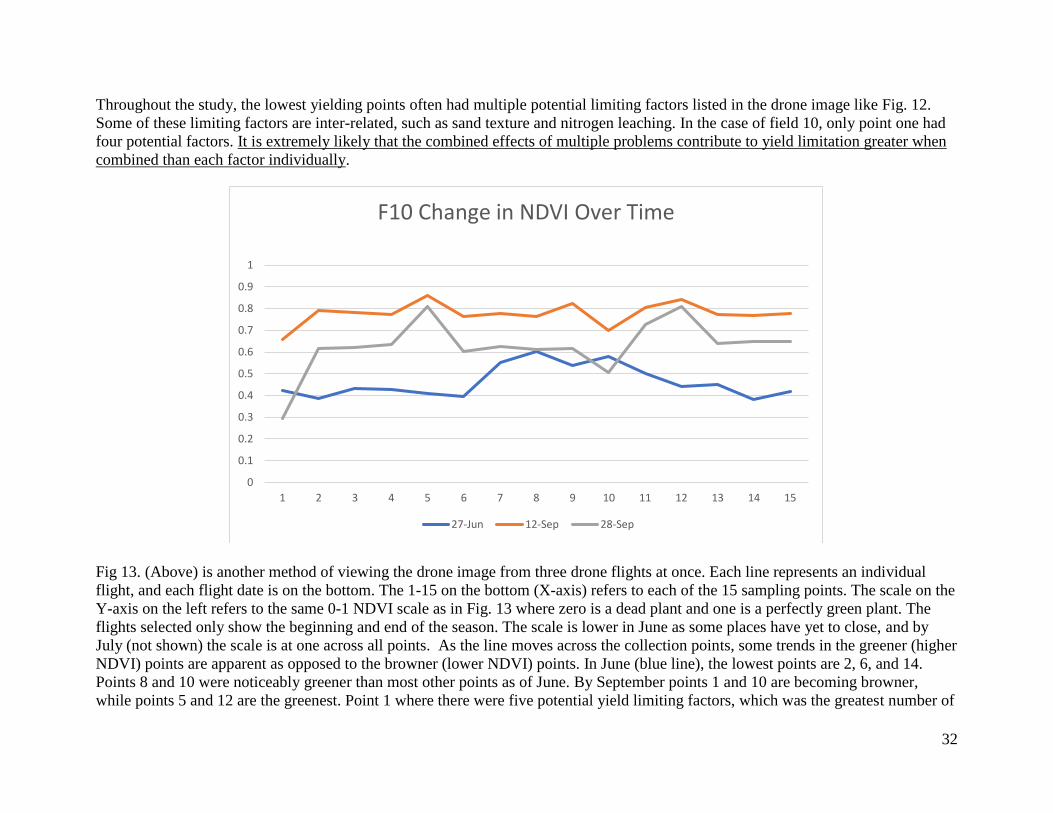
Fig. 14 (above) shows the total yield (after rot and green tubers removed) by size category. Each color represents a specific tuber size
profile. For example, yellow bars near the top indicate the 10-11.9 oz tuber size. The yield is measured in hundredweight per acre
(Cwt/A) on the right side, and the harvest date was the first week in September.
The lowest yielding sampling point numerically was point 12. In Fig. 12, this place in the field was noted as having compaction, low
soil sulfur and nitrogen at mid bulking. In Fig. 13, this point didn’t have much of a numerical drop in NDVI value throughout
September. It is possible that the underlying causes of this low yield didn’t kill the plant or enhance early die based on the drone
results. In examining figure 14, it appears that the 3-6 oz and 6-10 oz are notably less than most other collection points. In the
combined analysis for all processing fields, high soil sulfur at mid bulking was associated with yield limitation for 3-6 oz and 6-10 oz.
It is quite possible that low soil sulfur also has a pronounced effect on these size categories based on observations from this field,
although not tested by the analysis. Soil nitrogen was also important negative yield impact in the 6-10 oz size category, although it
was excess soil nitrogen at row closure associated with less 6-10 oz tubers. In this field, it appears that less soil nitrogen at bulking
also contributed to lower yield. The exact effects of sulfur and nitrogen individually on yield are not able to be separated based on
observation or association with the partial least squares regression employed for all processing fields.
A final observation of note in field 10 is the high yielding sampling point was number seven, which was located in the south-central
part of the field. This collection point had one of the largest yields with numerically greater 10-12 oz tubers and >12 oz tubers. What is
notable aside from yield is that this point was not the greenest point in the drone flights and was limited by soil nitrogen at mid
bulking, compaction, and low organic matter. This point was not limited by sulfur. It is possible that a factor outside of the study was
part of the final yield, but the combination of nutrient limitations is interesting in terms of studying the effect of sulfur availability on
yield remediation as a practice that can be altered by grower practice to increase 10-12 oz yield.
35
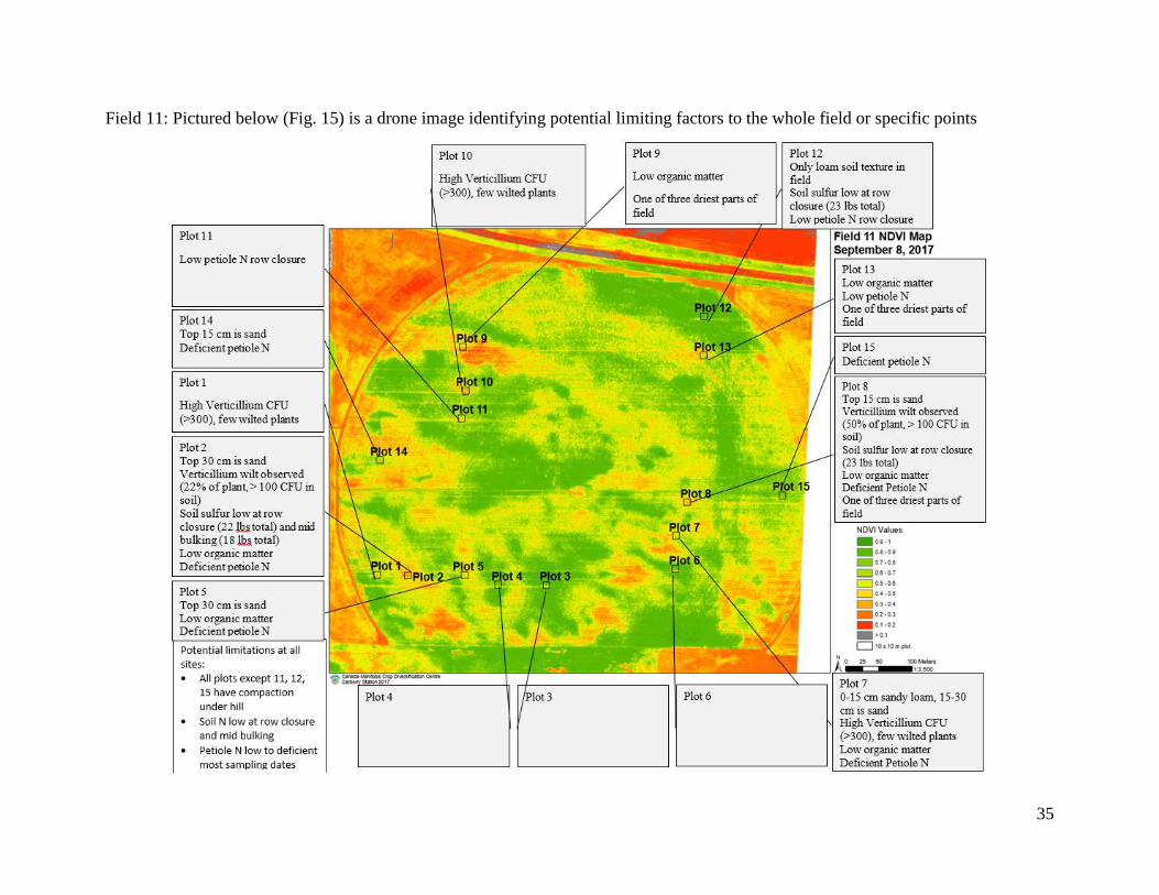
Field 11: Pictured below (Fig. 15) is a drone image identifying potential limiting factors to the whole field or specific points
36
In addition to evaluating the impact of variables on yield of fresh and processing fields together, individual fields from 2017 were
rated for nutrient, soil, disease, and plant health status. Drone imagery was used in conjunction with scouting, nutrient status as
determined by Agvise recommendations, and yield to visualize variability at each sampling point and what trends were apparent in the
overall yield. The point of this individual analysis is to demonstrate the usefulness of the Partial Least Square (PLS) analysis from all
processing fields in identifying one or a few major yield-limiting factors from a larger list of potential problems listed for a specific
site. This information begins the conversation with a local consultant and grower about priorities in remediating yield variability, and
ultimately develop practices to remediate the situation.
Plot numbers in the drone images refer to the 15 sampling points in each field. The top of each image is north in each field, and the
color scale refers to the NDVI values recorded by the drone. NDVI was recorded on a scale of 0-1, zero being red and refers to bare
earth, 1 refers to green tissue, and varying shades of green to yellow indicate senescencing plant matter. It is important to note that
weed canopy color will be recorded as well as potato, although no significant weed pressure was recorded in the sampling points in
field 11.
For each individual field, certain variables were identified as potential problems for the whole field or individual collection points that
could contribute to variable yield. Field 11 was observed to have compaction under the hill (beneath 30 cm/11.8 in from top of hill)
with an excess of 300 PSI. Compaction was not among the top ten most influential variables listed in the complete processing
analysis, indicating that it could be a problem on an individual field basis, but not among the worse problems across all processing
fields.
Very little Verticillium wilt was recorded in the field, with the most disease observed on the south side of the field in points 1, 2, 7,
and 8. Verticillium species counts exceeded 100 CFU /g in most points and >300 in points 1, 2, 7, and 10. It is generally accepted that
5-30 CFU/g of V. dahliae are necessary for infection. This plate count will encompass all Verticillium species, which doesn’t
accurately rely the number of V. dahliae CFU. Verticillium wilt will need to be monitored in the field and it could be a factor in
variable yield. The combined processing analysis indicated that the 10-12oz yield category is the size range most negatively impacted
by high Vertcillium counts, as severely infected plants are killed or debilitated during late bulking when tubers are sizing in this range.
Concern about any drops in 10-12 oz yield should consider the Verticillium counts in future years based on this information.
The main indicators of variable yield, among the variables recorded for the study, in this field are low soil nitrogen and sulfur in
petioles and soil throughout the production season. Low soil nitrogen was recorded across all collection points at row closure and mid
bulking, whereas low soil sulfur was a more sporadic problem with no obvious trend. Both sulfur and nitrogen were important
nutrients involved in variable yield across all processing fields, and lower yield was associated with lower nitrogen or sulfur. In this
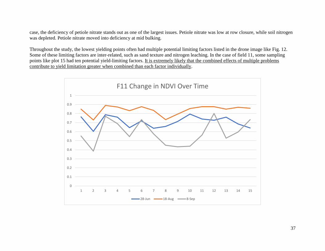
37
case, the deficiency of petiole nitrate stands out as one of the largest issues. Petiole nitrate was low at row closure, while soil nitrogen
was depleted. Petiole nitrate moved into deficiency at mid bulking.
Throughout the study, the lowest yielding points often had multiple potential limiting factors listed in the drone image like Fig. 12.
Some of these limiting factors are inter-related, such as sand texture and nitrogen leaching. In the case of field 11, some sampling
points like plot 15 had ten potential yield-limiting factors. It is extremely likely that the combined effects of multiple problems
contribute to yield limitation greater when combined than each factor individually.
0
0.1
0.2
0.3
0.4
0.5
0.6
0.7
0.8
0.9
1
1 2 3 4 5 6 7 8 9 10 11 12 13 14 15
F11 Change in NDVI Over Time
28-Jun 18-Aug 8-Sep
38
Fig 16. (Above) is another method of viewing the drone image from three drone flights at once. Each line represents an individual
flight, and each flight date is on the bottom. The 1-15 on the bottom (X-axis) refers to each of the 15 sampling points. The scale on the
Y-axis on the left refers to the same 0-1 NDVI scale as in Fig. 15 where zero is a dead plant and one is a perfectly green plant. The
flights selected only show the beginning and end of the season. The scale is lower in June as some places have yet to close, and by
July (not shown) the scale is at one across all points. As the line moves across the collection points, some trends in the greener (higher
NDVI) points are apparent as opposed to the browner (lower NDVI) points. In June (blue line), the lowest points are 2, 5, 7, and 15.
Points 3 and 10 were noticeably greener than most other points as of June. By September points 2, 8-10, and 13 are becoming
browner, while points 3, 6, and 12 are the greenest. In the case of this field, no clear trend was apparent in June or July to identify
which point would see the greatest decrease in NDVI as September progressed. Sampling points 2, 5, 7, 8, 12, and 13 had multiple
yield-limiting factors observed throughout the production season in Fig. 15. These sampling points with many factors associated with
yield limitations were present and the point had noticeably lower NDVI as of June. In these fields, the NDVI recovered to 1 as of July,
but the same pattern of decreased NDVI returned in August and became more pronounced into September. In these cases, a drone
flight in June may identify areas where the canopy will die prematurely in August with a NDVI value that is already low in June, but
the level of greenness is not necessarily discernable to the human eye on the ground. This interesting observation will absolutely be
the subject of more study in the variability project.
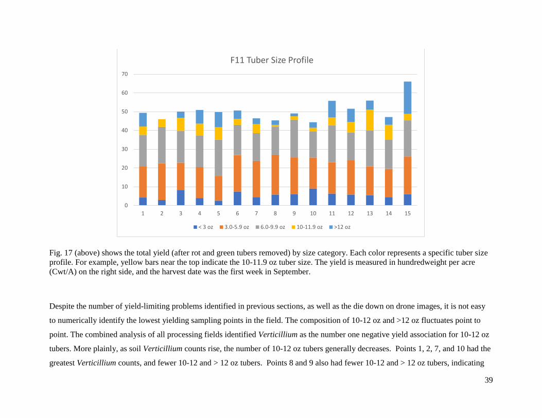
39
Fig. 17 (above) shows the total yield (after rot and green tubers removed) by size category. Each color represents a specific tuber size
profile. For example, yellow bars near the top indicate the 10-11.9 oz tuber size. The yield is measured in hundredweight per acre
(Cwt/A) on the right side, and the harvest date was the first week in September.
Despite the number of yield-limiting problems identified in previous sections, as well as the die down on drone images, it is not easy
to numerically identify the lowest yielding sampling points in the field. The composition of 10-12 oz and >12 oz fluctuates point to
point. The combined analysis of all processing fields identified Verticillium as the number one negative yield association for 10-12 oz
tubers. More plainly, as soil Verticillium counts rise, the number of 10-12 oz tubers generally decreases. Points 1, 2, 7, and 10 had the
greatest Verticillium counts, and fewer 10-12 and > 12 oz tubers. Points 8 and 9 also had fewer 10-12 and > 12 oz tubers, indicating
0
10
20
30
40
50
60
70
1 2 3 4 5 6 7 8 9 10 11 12 13 14 15
F11 Tuber Size Profile
< 3 oz 3.0-5.9 oz 6.0-9.9 oz 10-11.9 oz >12 oz
40
more than Verticillium needs to be considered. Points 8 and 9 also had low organic matter and soil moisture throughout the season, in
addition to the nitrogen problems outlined earlier. These factors could contribute to the fewer 10-12 and > 12 oz tubers.
It is relatively easier to look at Fig. 14 and identify point 15 as the numerically greatest yield. It appears that there were many > 12 oz
tubers in this point in the far east of the field. The list of potential problems is also shorter at point 15, and only includes the nitrogen
problems previously mentioned. The combined analysis of all processing fields associates more >12 oz yield with less soil nitrogen at
row closure and more soil sulfur at row closure. The nitrogen problems at this point could have been of benefit in not providing excess
nitrogen, and the availability of sulfur could have improved the >12 oz yield in this point. However, field notes indicate the entire field
was recently extended eastward. This sampling point is likely to have a different cropping history than the remainder of the field that
was not included in this study that could contribute to the >12 oz yield.

41
Field 12 Pictured below (Fig. 18) is a drone image identifying potential limiting factors to the whole field or specific points

42
In addition to evaluating the impact of variables on yield of fresh and processing fields together, individual fields from 2017 were
rated for nutrient, soil, disease, and plant health status. Drone imagery was used in conjunction with scouting, nutrient status as
determined by Agvise recommendations, and yield to visualize variability at each sampling point and what trends were apparent in the
overall yield. The point of this individual analysis is to demonstrate the usefulness of the Partial Least Square (PLS) analysis from all
processing fields in identifying one or a few major yield-limiting factors from a larger list of potential problems listed for a specific
site. This information begins the conversation with a local consultant and grower about priorities in remediating yield variability, and
ultimately develop practices to remediate the situation.
Plot numbers in the drone images refer to the 15 sampling points in each field. The top of each image is north in each field, and the
color scale refers to the NDVI values recorded by the drone. NDVI was recorded on a scale of 0-1, zero being red and refers to bare
earth, 1 refers to green tissue, and varying shades of green to yellow indicate senescencing plant matter. It is important to note that
weed canopy color will be recorded as well as potato, and all points in the northern half of the field were noted to have eastern black
nightshade.
For each individual field, certain variables were identified as potential problems for the whole field or individual collection points that
could contribute to variable yield. Field 12 was observed to have compaction under the hill (beneath 30 cm/11.8 in from top of hill)
with an excess of 300 PSI. Compaction was not among the top ten most influential variables listed in the complete processing
analysis, indicating that it could be a problem on an individual field basis, but not among the worse problems across all processing
fields.
Very little Verticillium wilt was recorded in the field, with the most disease observed on the south side of the field in point 8.
Verticillium species counts exceeded 100 CFU /g in plot 8. Wilt was only observed in plot 12, which had a low (28 CFU) count. It is
generally accepted that 5-30 CFU/g of V. dahliae are necessary for infection. This plate count will encompass all Verticillium species,
which doesn’t accurately rely the number of V. dahliae CFU. Verticillium wilt will need to be monitored in the field and it could be a
factor in variable yield. The combined processing analysis indicated that the 10-12 oz yield category is the size range most negatively
impacted by high Verticillium counts, as severely infected plants are killed or debilitated during late bulking when tubers are sizing in
this range. Concern about any drops in 10-12 oz yield should consider the Verticillium counts in future years based on this
information. Eastern black nightshade was noted as a problem in most collection points on the north side of the field. There is a known
interaction with Verticillium and nightshade where nightshade is not only a host, but also trains the Verticillium to be aggressive on
potato. As the Verticillium becomes aggressive to potato, lower counts are necessary to induce higher levels of disease. Nightshade
control then becomes another factor to keep in mind for this specific field but will be overlooked by the total analysis of combined
processing fields because nightshade wasn’t present in all fields.
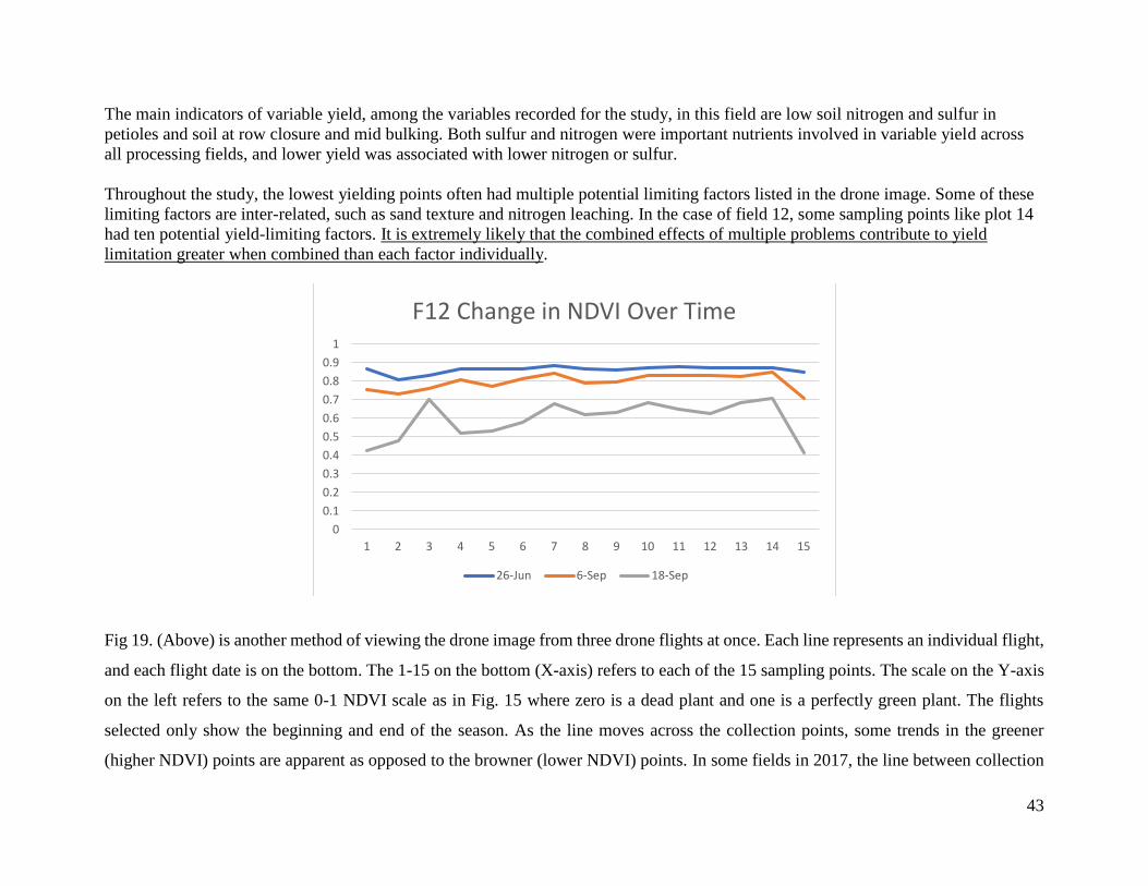
43
The main indicators of variable yield, among the variables recorded for the study, in this field are low soil nitrogen and sulfur in
petioles and soil at row closure and mid bulking. Both sulfur and nitrogen were important nutrients involved in variable yield across
all processing fields, and lower yield was associated with lower nitrogen or sulfur.
Throughout the study, the lowest yielding points often had multiple potential limiting factors listed in the drone image. Some of these
limiting factors are inter-related, such as sand texture and nitrogen leaching. In the case of field 12, some sampling points like plot 14
had ten potential yield-limiting factors. It is extremely likely that the combined effects of multiple problems contribute to yield
limitation greater when combined than each factor individually.
Fig 19. (Above) is another method of viewing the drone image from three drone flights at once. Each line represents an individual flight,
and each flight date is on the bottom. The 1-15 on the bottom (X-axis) refers to each of the 15 sampling points. The scale on the Y-axis
on the left refers to the same 0-1 NDVI scale as in Fig. 15 where zero is a dead plant and one is a perfectly green plant. The flights
selected only show the beginning and end of the season. As the line moves across the collection points, some trends in the greener
(higher NDVI) points are apparent as opposed to the browner (lower NDVI) points. In some fields in 2017, the line between collection
0
0.1
0.2
0.3
0.4
0.5
0.6
0.7
0.8
0.9
1
1 2 3 4 5 6 7 8 9 10 11 12 13 14 15
F12 Change in NDVI Over Time
26-Jun 6-Sep 18-Sep

44
points was similar in June as it was in September, indicating we can see the weaker sampling points via drone flight months before early
die sets in. Your field is a counter example where the lowest (less green) sampling point in June (plot 2) was not the lowest point in
September. Additionally, plot 14 had numerous yield-limiting factors associated with it and yet was one of the greenest points. More
research would be necessary to develop the June drone image as a predictive tool for early die.
Fig. 20 (above) shows the total yield (after rot and green tubers removed) by size category. Each color represents a specific tuber size
profile. For example, yellow bars near the top indicate the 10-11.9 oz tuber size. The yield is measured in hundredweight per acre
(Cwt/A) on the right side, and the harvest date was the first week in September.
Despite the number of yield-limiting problems identified in previous sections, as well as the die down on drone images, it is not easy
to numerically identify the lowest yielding sampling points in the field. Without statistics, it appears that point 14 is has the lowest
0
10
20
30
40
50
60
70
1 2 3 4 5 6 7 8 9 10 11 12 13 14 15
F12 Tuber Size Profile
< 3 oz 3.0-5.9 oz 6.0-9.9 oz 10-11.9 oz >12 oz
45
total yield and all size categories are less than the remaining points. Plot 14 had six possible yield-limiting factors identified though
soil and petiole samples for the project. Plot 14 also had many Eastern Black Nightshade plants that could reduce yield. The highest
yielding points (numerically) were sites 10 and 13, which had few to no potential yield-limiting factors identified.

46
Field 13 Pictured below (Fig. 21) is a drone image identifying potential limiting factors to the whole field or specific points

47
In addition to evaluating the impact of variables on yield of fresh and processing fields together, individual fields from 2017 were
rated for nutrient, soil, disease, and plant health status. Drone imagery was used in conjunction with scouting, nutrient status as
determined by Agvise recommendations, and yield to visualize variability at each sampling point and what trends were apparent in the
overall yield. The point of this individual analysis is to demonstrate the usefulness of the Partial Least Square (PLS) analysis from all
processing fields in identifying one or a few major yield-limiting factors from a larger list of potential problems listed for a specific
site. This information begins the conversation with a local consultant and grower about priorities in remediating yield variability, and
ultimately develop practices to remediate the situation.
Plot numbers in the drone images refer to the 15 sampling points in each field. The top of each image is north in each field, and the
color scale refers to the NDVI values recorded by the drone. NDVI was recorded on a scale of 0-1, zero being red and refers to bare
earth, 1 refers to green tissue, and varying shades of green to yellow indicate senescencing plant matter. It is important to note that
weed canopy color will be recorded as well as potato, and all points in the northern half of the field were noted to have eastern black
nightshade.
For each individual field, certain variables were identified as potential problems for the whole field or individual collection points that
could contribute to variable yield. Field 13 was generally sandy loam, but only two points of 2 and 13 had sand texture. Sand points
were generally the driest points in the field. Little Verticillium and few points of compaction were observed, which is unusual for this
experiment. Chlorosis unlikely to be Verticillium wilt as most points were under 30 CFU/g, which is theoretically capable of causing
disease but not often observed in the field.
The main indicators of variable yield, among the variables recorded for the study, in this field are low soil nitrogen and sulfur in
petioles and soil at row closure and mid bulking. Both sulfur and nitrogen were important nutrients involved in variable yield across
all processing fields, and lower yield was associated with lower nitrogen or sulfur.
Throughout the study, the lowest yielding points often had multiple potential limiting factors listed in the drone image. Some of these
limiting factors are inter-related, such as sand texture and nitrogen leaching. In the case of field 13, some sampling points like plot 2
had six potential yield-limiting factors. It is extremely likely that the combined effects of multiple problems contribute to yield
limitation greater when combined than each factor individually.
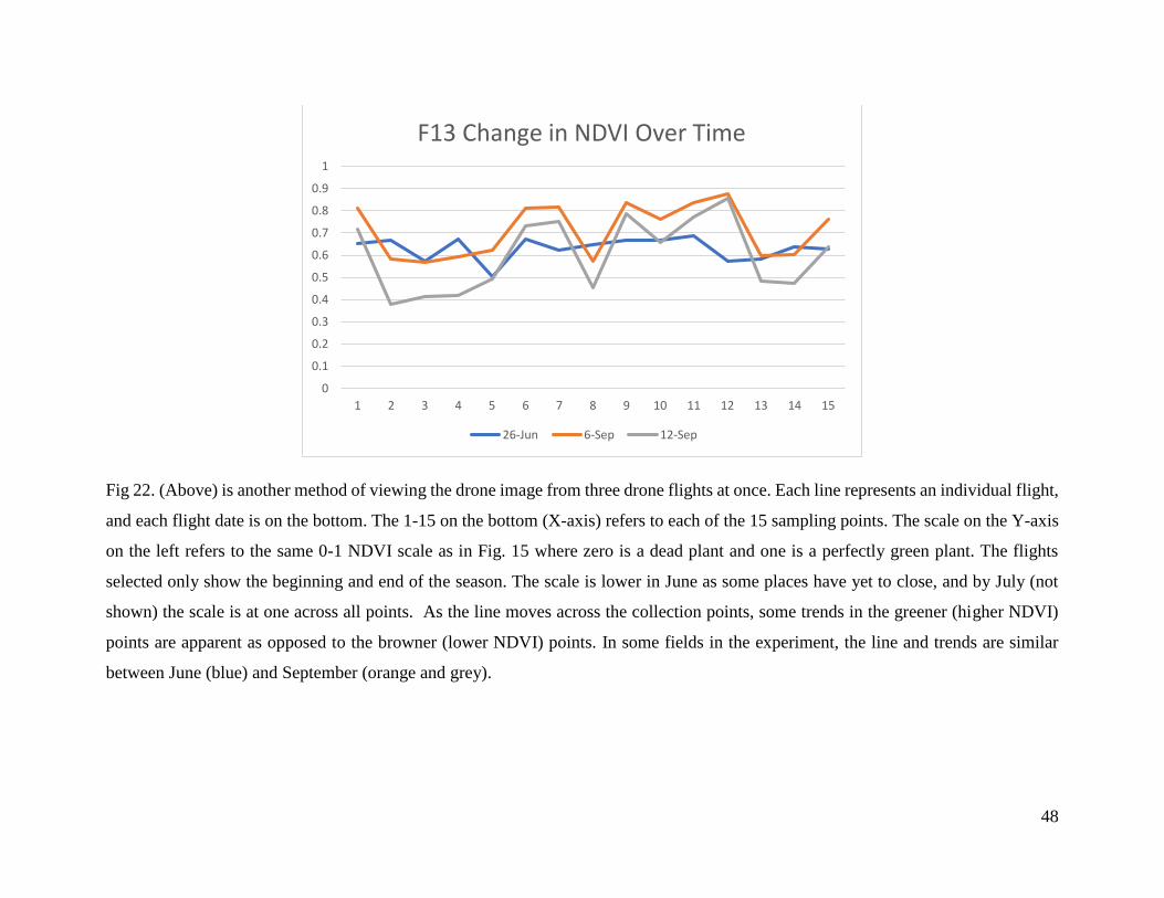
48
Fig 22. (Above) is another method of viewing the drone image from three drone flights at once. Each line represents an individual flight,
and each flight date is on the bottom. The 1-15 on the bottom (X-axis) refers to each of the 15 sampling points. The scale on the Y-axis
on the left refers to the same 0-1 NDVI scale as in Fig. 15 where zero is a dead plant and one is a perfectly green plant. The flights
selected only show the beginning and end of the season. The scale is lower in June as some places have yet to close, and by July (not
shown) the scale is at one across all points. As the line moves across the collection points, some trends in the greener (higher NDVI)
points are apparent as opposed to the browner (lower NDVI) points. In some fields in the experiment, the line and trends are similar
between June (blue) and September (orange and grey).
0
0.1
0.2
0.3
0.4
0.5
0.6
0.7
0.8
0.9
1
1 2 3 4 5 6 7 8 9 10 11 12 13 14 15
F13 Change in NDVI Over Time
26-Jun 6-Sep 12-Sep
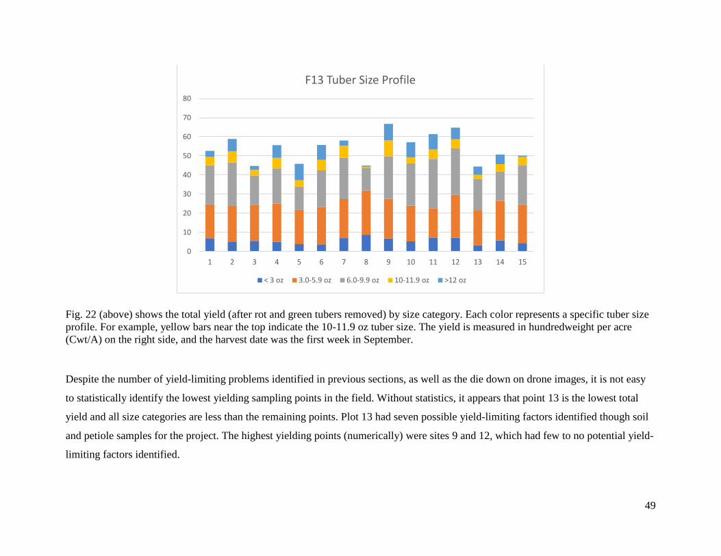
49
Fig. 22 (above) shows the total yield (after rot and green tubers removed) by size category. Each color represents a specific tuber size
profile. For example, yellow bars near the top indicate the 10-11.9 oz tuber size. The yield is measured in hundredweight per acre
(Cwt/A) on the right side, and the harvest date was the first week in September.
Despite the number of yield-limiting problems identified in previous sections, as well as the die down on drone images, it is not easy
to statistically identify the lowest yielding sampling points in the field. Without statistics, it appears that point 13 is the lowest total
yield and all size categories are less than the remaining points. Plot 13 had seven possible yield-limiting factors identified though soil
and petiole samples for the project. The highest yielding points (numerically) were sites 9 and 12, which had few to no potential yield-
limiting factors identified.
0
10
20
30
40
50
60
70
80
1 2 3 4 5 6 7 8 9 10 11 12 13 14 15
F13 Tuber Size Profile
< 3 oz 3.0-5.9 oz 6.0-9.9 oz 10-11.9 oz >12 oz
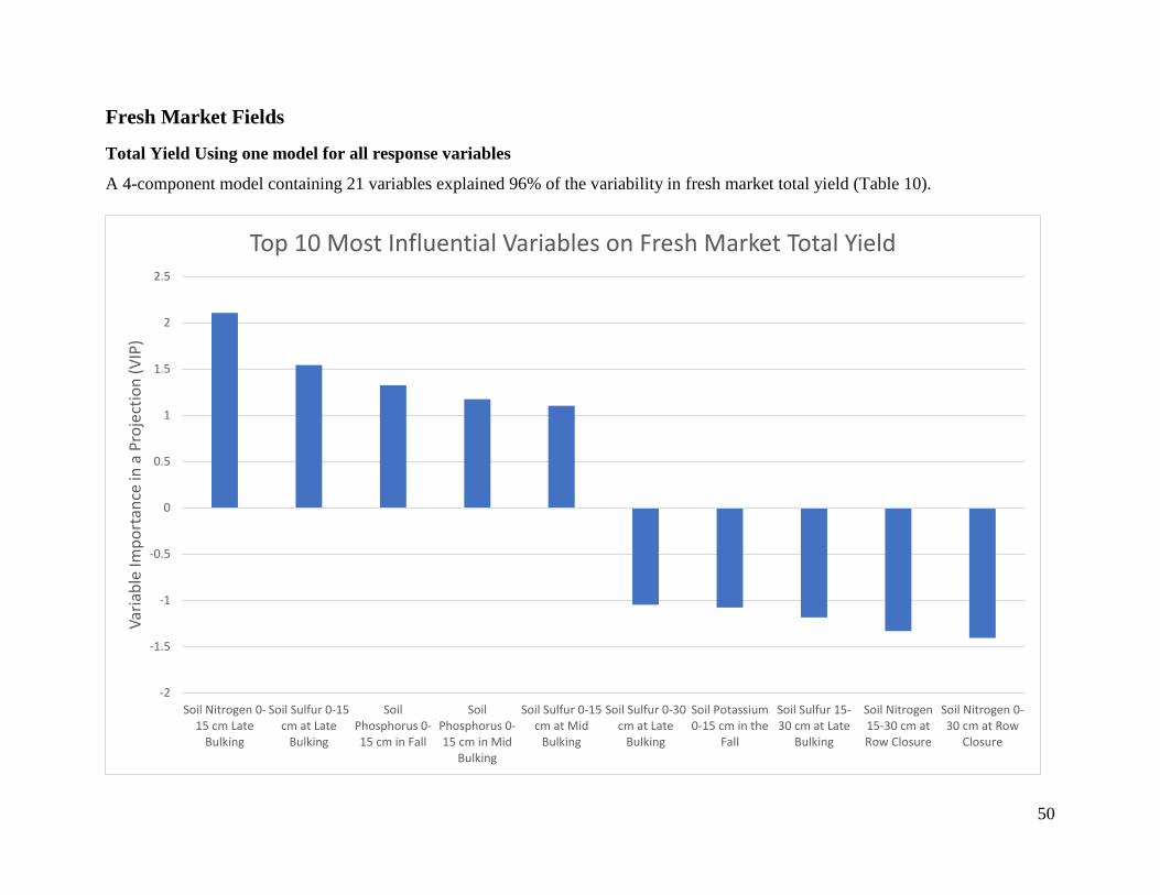
50
Fresh Market Fields
Total Yield Using one model for all response variables
A 4-component model containing 21 variables explained 96% of the variability in fresh market total yield (Table 10).
-2
-1.5
-1
-0.5
0
0.5
1
1.5
2
2.5
Soil Nitrogen 0-15 cm Late
Bulking
Soil Sulfur 0-15cm at Late
Bulking
SoilPhosphorus 0-15 cm in Fall
SoilPhosphorus 0-15 cm in Mid
Bulking
Soil Sulfur 0-15cm at Mid
Bulking
Soil Sulfur 0-30cm at Late
Bulking
Soil Potassium0-15 cm in the
Fall
Soil Sulfur 15-30 cm at Late
Bulking
Soil Nitrogen15-30 cm atRow Closure
Soil Nitrogen 0-30 cm at Row
Closure
Var
iab
le Im
po
rtan
ce in
a P
roje
ctio
n (
VIP
)
Top 10 Most Influential Variables on Fresh Market Total Yield
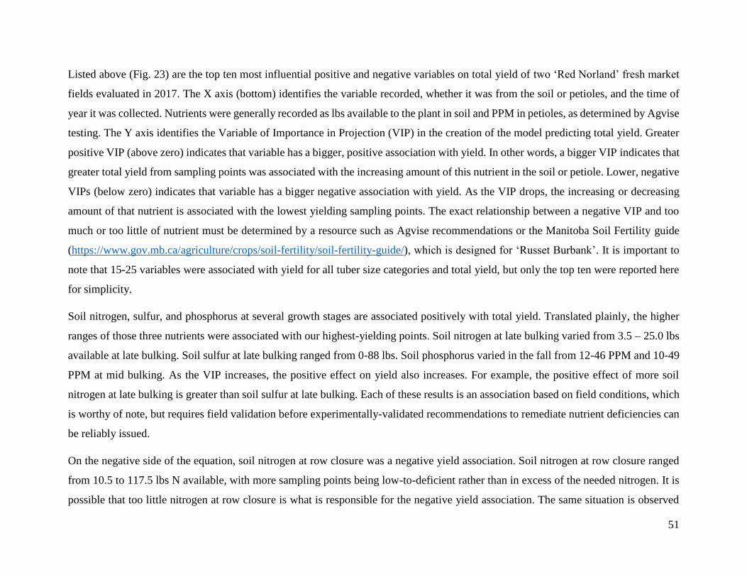
51
Listed above (Fig. 23) are the top ten most influential positive and negative variables on total yield of two ‘Red Norland’ fresh market
fields evaluated in 2017. The X axis (bottom) identifies the variable recorded, whether it was from the soil or petioles, and the time of
year it was collected. Nutrients were generally recorded as lbs available to the plant in soil and PPM in petioles, as determined by Agvise
testing. The Y axis identifies the Variable of Importance in Projection (VIP) in the creation of the model predicting total yield. Greater
positive VIP (above zero) indicates that variable has a bigger, positive association with yield. In other words, a bigger VIP indicates that
greater total yield from sampling points was associated with the increasing amount of this nutrient in the soil or petiole. Lower, negative
VIPs (below zero) indicates that variable has a bigger negative association with yield. As the VIP drops, the increasing or decreasing
amount of that nutrient is associated with the lowest yielding sampling points. The exact relationship between a negative VIP and too
much or too little of nutrient must be determined by a resource such as Agvise recommendations or the Manitoba Soil Fertility guide
(https://www.gov.mb.ca/agriculture/crops/soil-fertility/soil-fertility-guide/), which is designed for ‘Russet Burbank’. It is important to
note that 15-25 variables were associated with yield for all tuber size categories and total yield, but only the top ten were reported here
for simplicity.
Soil nitrogen, sulfur, and phosphorus at several growth stages are associated positively with total yield. Translated plainly, the higher
ranges of those three nutrients were associated with our highest-yielding points. Soil nitrogen at late bulking varied from 3.5 – 25.0 lbs
available at late bulking. Soil sulfur at late bulking ranged from 0-88 lbs. Soil phosphorus varied in the fall from 12-46 PPM and 10-49
PPM at mid bulking. As the VIP increases, the positive effect on yield also increases. For example, the positive effect of more soil
nitrogen at late bulking is greater than soil sulfur at late bulking. Each of these results is an association based on field conditions, which
is worthy of note, but requires field validation before experimentally-validated recommendations to remediate nutrient deficiencies can
be reliably issued.
On the negative side of the equation, soil nitrogen at row closure was a negative yield association. Soil nitrogen at row closure ranged
from 10.5 to 117.5 lbs N available, with more sampling points being low-to-deficient rather than in excess of the needed nitrogen. It is
possible that too little nitrogen at row closure is what is responsible for the negative yield association. The same situation is observed
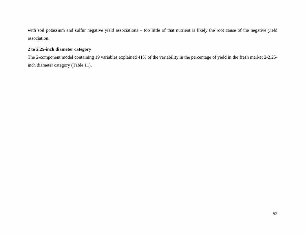
52
with soil potassium and sulfur negative yield associations – too little of that nutrient is likely the root cause of the negative yield
association.
2 to 2.25-inch diameter category
The 2-component model containing 19 variables explained 41% of the variability in the percentage of yield in the fresh market 2-2.25-
inch diameter category (Table 11).
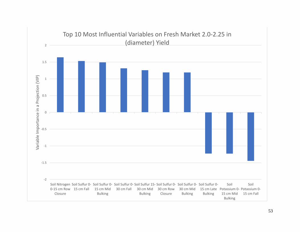
53
-2
-1.5
-1
-0.5
0
0.5
1
1.5
2
Soil Nitrogen0-15 cm Row
Closure
Soil Sulfur 0-15 cm Fall
Soil Sulfur 0-15 cm Mid
Bulking
Soil Sulfur 0-30 cm Fall
Soil Sulfur 15-30 cm Mid
Bulking
Soil Sulfur 0-30 cm Row
Closure
Soil Sulfur 0-30 cm Mid
Bulking
Soil Sulfur 0-15 cm Late
Bulking
SoilPotassium 0-
15 cm MidBulking
SoilPotassium 0-
15 cm Fall
Var
iab
le Im
po
rtan
ce in
a P
roje
ctio
n (
VIP
)Top 10 Most Influential Variables on Fresh Market 2.0-2.25 in
(diameter) Yield

54
Listed above (Fig. 24) are the top ten most influential positive and negative variables on total yield of two ‘Red Norland’ fresh market
fields evaluated in 2017. The X axis (bottom) identifies the variable recorded, whether it was from the soil or petioles, and the time of
year it was collected. Nutrients were generally recorded as lbs available to the plant in soil and PPM in petioles, as determined by Agvise
testing. The Y axis identifies the Variable of Importance in Projection (VIP) in the creation of the model predicting total yield. Greater
positive VIP (above zero) indicates that variable has a bigger, positive association with yield. In other words, a bigger VIP indicates that
greater total yield from sampling points was associated with the increasing amount of this nutrient in the soil or petiole. Lower, negative
VIPs (below zero) indicates that variable has a bigger negative association with yield.
Soil nitrogen and sulfur at several growth stages are associated positively with total yield. Translated plainly, the higher ranges of those
nutrients were associated with our highest-yielding points. Soil nitrogen at row closure ranged from 10.5 to 117.5 lbs N available, with
more sampling points being low-to-deficient rather than in excess of the needed nitrogen. Soil sulfur varied from 0-120 lbs available in
the soil throughout the sampling date from row closure to fall soil sampling (postharvest), which would range from deficient to very
high for ‘Russet Burbanks’. The positive yield association points to the higher ranges (40-60 lbs were common high observations in the
experiment) as the likely yield-benefitting range, but field experimentation is needed to identify this exact range and the best practices
to get there. This is especially important given our range of quality was determined for another cultivar other than ‘Red Norland’. The
negative yield associations for sulfur and potassium likely originate from soil samples deficient in these nutrients.
2.25 to 3.0-inch diameter category
The 2-component model containing 17 variables explained 52% of the variability in the percentage of yield in the fresh market 2.25 to
3.0-inch diameter category (Table 12).
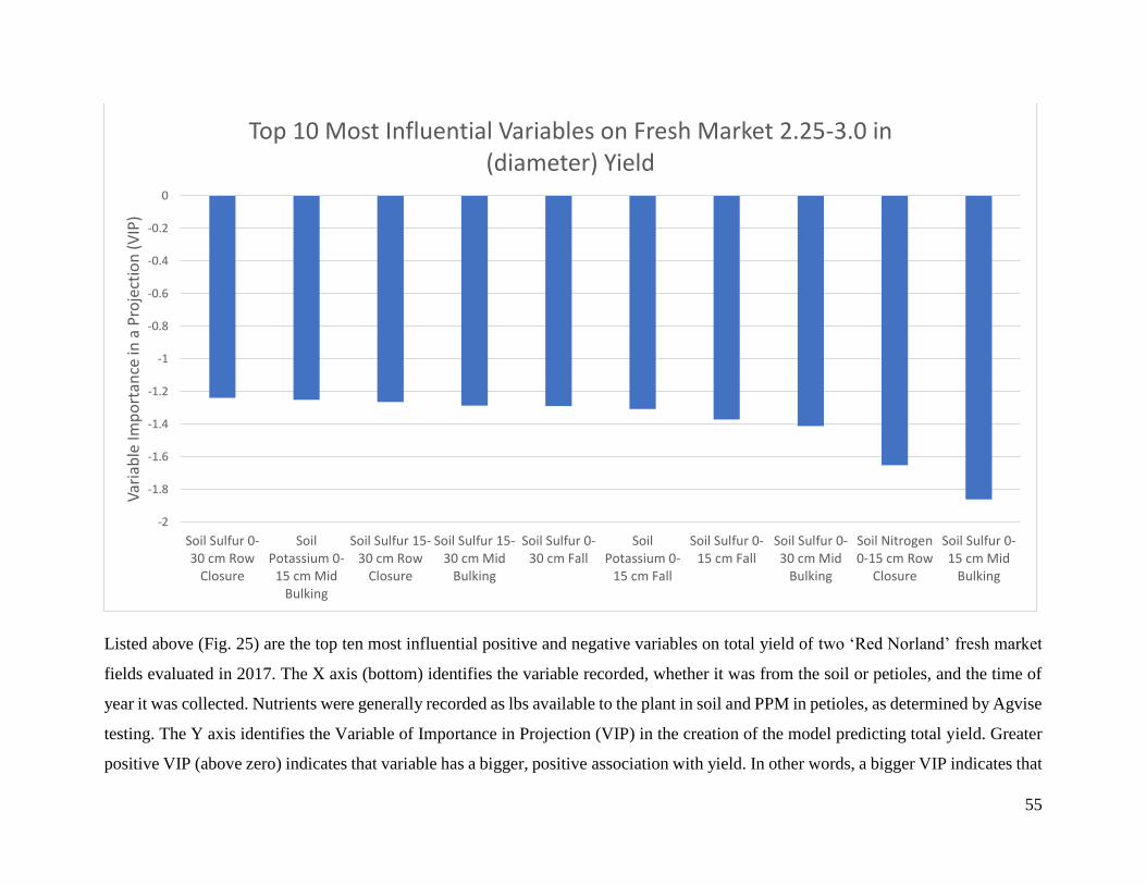
55
Listed above (Fig. 25) are the top ten most influential positive and negative variables on total yield of two ‘Red Norland’ fresh market
fields evaluated in 2017. The X axis (bottom) identifies the variable recorded, whether it was from the soil or petioles, and the time of
year it was collected. Nutrients were generally recorded as lbs available to the plant in soil and PPM in petioles, as determined by Agvise
testing. The Y axis identifies the Variable of Importance in Projection (VIP) in the creation of the model predicting total yield. Greater
positive VIP (above zero) indicates that variable has a bigger, positive association with yield. In other words, a bigger VIP indicates that
-2
-1.8
-1.6
-1.4
-1.2
-1
-0.8
-0.6
-0.4
-0.2
0
Soil Sulfur 0-30 cm Row
Closure
SoilPotassium 0-
15 cm MidBulking
Soil Sulfur 15-30 cm Row
Closure
Soil Sulfur 15-30 cm Mid
Bulking
Soil Sulfur 0-30 cm Fall
SoilPotassium 0-
15 cm Fall
Soil Sulfur 0-15 cm Fall
Soil Sulfur 0-30 cm Mid
Bulking
Soil Nitrogen0-15 cm Row
Closure
Soil Sulfur 0-15 cm Mid
Bulking
Var
iab
le Im
po
rtan
ce in
a P
roje
ctio
n (
VIP
)Top 10 Most Influential Variables on Fresh Market 2.25-3.0 in
(diameter) Yield

56
greater total yield from sampling points was associated with the increasing amount of this nutrient in the soil or petiole. Lower, negative
VIPs (below zero) indicates that variable has a bigger negative association with yield.
These results are unusual in that this is the only size category in the whole experiment, fresh market or processing, where the top 10
most influential variables were all negative. Based on previous results with nitrogen, potassium, and sulfur in the soil, low to deficient
soil status is a likely culprit for the negative yield association.
3.0 to 3.5-inch diameter category
The 2-component model containing 22 variables explained 78% of the variability in the percentage of yield in the fresh market 3.0 to
3.5-inch diameter category.
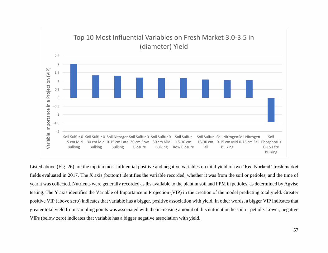
57
Listed above (Fig. 26) are the top ten most influential positive and negative variables on total yield of two ‘Red Norland’ fresh market
fields evaluated in 2017. The X axis (bottom) identifies the variable recorded, whether it was from the soil or petioles, and the time of
year it was collected. Nutrients were generally recorded as lbs available to the plant in soil and PPM in petioles, as determined by Agvise
testing. The Y axis identifies the Variable of Importance in Projection (VIP) in the creation of the model predicting total yield. Greater
positive VIP (above zero) indicates that variable has a bigger, positive association with yield. In other words, a bigger VIP indicates that
greater total yield from sampling points was associated with the increasing amount of this nutrient in the soil or petiole. Lower, negative
VIPs (below zero) indicates that variable has a bigger negative association with yield.
-2
-1.5
-1
-0.5
0
0.5
1
1.5
2
2.5
Soil Sulfur 0-15 cm Mid
Bulking
Soil Sulfur 0-30 cm Mid
Bulking
Soil Nitrogen0-15 cm Late
Bulking
Soil Sulfur 0-30 cm Row
Closure
Soil Sulfur 0-30 cm Mid
Bulking
Soil Sulfur15-30 cm
Row Closure
Soil Sulfur15-30 cm
Fall
Soil Nitrogen0-15 cm Mid
Bulking
Soil Nitrogen0-15 cm Fall
SoilPhosphorus
0-15 LateBulking
Var
iab
le Im
po
rtan
ce in
a P
roje
ctio
n (
VIP
)
Top 10 Most Influential Variables on Fresh Market 3.0-3.5 in (diameter) Yield
58
The interpretation of these results is that higher ranges of soil sulfur and nitrogen at several growth stages have positive yield associations
with these larger tubers. Interestingly, the soil sulfur at mid bulking has the strongest, positive yield association of all the growth stages.
This is very consistent with previous results for smaller diameter tubers and even total yield. Consistency is important in evaluating the
quality of the results of any study, this one included. Based on previous results with potassium in the soil, low to deficient soil status is
a likely culprit for the negative yield association.
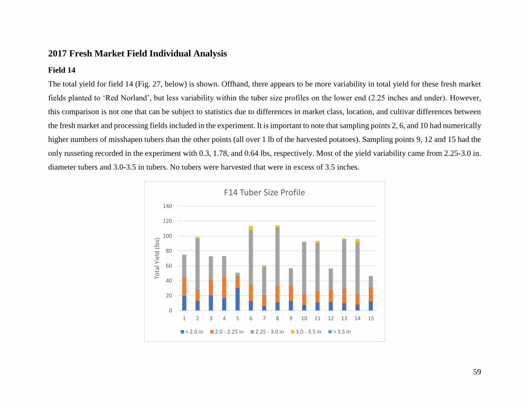
59
2017 Fresh Market Field Individual Analysis
Field 14
The total yield for field 14 (Fig. 27, below) is shown. Offhand, there appears to be more variability in total yield for these fresh market
fields planted to ‘Red Norland’, but less variability within the tuber size profiles on the lower end (2.25 inches and under). However,
this comparison is not one that can be subject to statistics due to differences in market class, location, and cultivar differences between
the fresh market and processing fields included in the experiment. It is important to note that sampling points 2, 6, and 10 had numerically
higher numbers of misshapen tubers than the other points (all over 1 lb of the harvested potatoes). Sampling points 9, 12 and 15 had the
only russeting recorded in the experiment with 0.3, 1.78, and 0.64 lbs, respectively. Most of the yield variability came from 2.25-3.0 in.
diameter tubers and 3.0-3.5 in tubers. No tubers were harvested that were in excess of 3.5 inches.
0
20
40
60
80
100
120
140
1 2 3 4 5 6 7 8 9 10 11 12 13 14 15
Tota
l Yie
ld (
lbs)
F14 Tuber Size Profile
< 2.0 in 2.0 - 2.25 in 2.25 - 3.0 in 3.0 - 3.5 in > 3.5 in
60
Fig. 27 Total yield of field 14 (‘Red Norland’) in lbs for each of the 15 sampling points. The colors denote the lbs of each size
category recorded in the one 10-meter harvest row of each sampling point.
The following page will have a bare earth drone image from the start of the season of field 14 (Fig. 28). The image identifies where
the 15 sampling points were placed in the field and list potential yield-limiting variables. It is important to note that the
recommendations were for ‘Russet Burbank’, and differences will exist between the needs of different cultivars destined for different
market classes.
The Verticillium counts are particularly noteworthy for this field in that points 8, 10, 11, and 13 had counts in excess of 100 CFU/g
soil (CFU colony forming units – a measure determined by growth on a petri plate. This is important because dead or growth-inhibited
colony forming units are of no threat). This result is peculiar in that these sampling points because they were also some of the highest
yielding (Fig. 27). Verticillium wilt generally reduced the larger (10-12 oz) tubers from ‘Russet Burbank’, thereby reducing the total
yield and value of a sampling point. There is no obvious answer why that did not happen here. It is generally accepted that 5-30 CFU
of Verticillium dahliae are necessary to infect most Verticillium wilt-susceptible russet varieties. The counts provided on this analysis
do not reliably differentiate between Verticillium species, implying that high counts are likely a mixture of species. However, the
probability of exceeding the 5-30 CFU of V. dahliae is greater when the total Verticillium species count is in excess of 100 or 200.
While the effect of Verticillium wilt may not be discernable for subsequent potato rotations, these areas of the field with high counts
risk Verticillium wilt-related economic loss in the long term if no form of management is ever enacted. Verticillium is the kind of
problem that builds with time, especially on the scale of decades. As the problem can take a long time to build, it may be possible to
enact small management changes that also work over the long scale at which Verticillium is operating on.
The lowest yielding sampling points in this field, such as points 5, 7, 9, 12, and 15, were recorded as low to deficient petiole N at mid
bulking. Granted, the scale of low to deficient was set for ‘Russet Burbank’, not ‘Red Norland’. However, Burbank yield of larger (10-
12 oz tubers) and total yield decreased when nitrogen deficiencies were noted in the petiole or soil. It is possible that the shortage of N
61
contributed to the lack of yield. It is also not impossible that another factor outside of the variables recorded in the experiment also
contributed to the lack of yield at these sampling points. This information would have to be combined with the grower and consultants
experience with this specific field in order to clarify if other explanations could exist for this specific field, but not both fresh market
fields included in this experiment.

62
Fig. 24
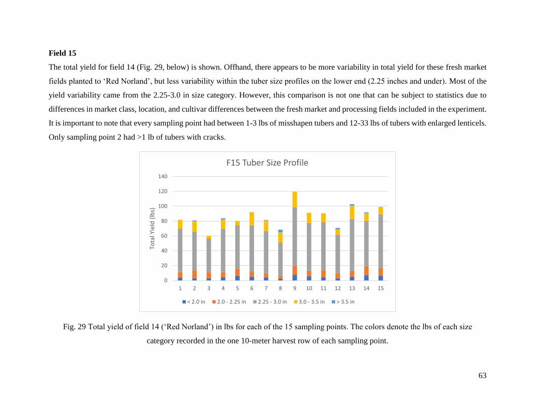
63
Field 15
The total yield for field 14 (Fig. 29, below) is shown. Offhand, there appears to be more variability in total yield for these fresh market
fields planted to ‘Red Norland’, but less variability within the tuber size profiles on the lower end (2.25 inches and under). Most of the
yield variability came from the 2.25-3.0 in size category. However, this comparison is not one that can be subject to statistics due to
differences in market class, location, and cultivar differences between the fresh market and processing fields included in the experiment.
It is important to note that every sampling point had between 1-3 lbs of misshapen tubers and 12-33 lbs of tubers with enlarged lenticels.
Only sampling point 2 had >1 lb of tubers with cracks.
Fig. 29 Total yield of field 14 (‘Red Norland’) in lbs for each of the 15 sampling points. The colors denote the lbs of each size
category recorded in the one 10-meter harvest row of each sampling point.
0
20
40
60
80
100
120
140
1 2 3 4 5 6 7 8 9 10 11 12 13 14 15
Tota
l Yie
ld (
lbs)
F15 Tuber Size Profile
< 2.0 in 2.0 - 2.25 in 2.25 - 3.0 in 3.0 - 3.5 in > 3.5 in
64
The following page will have a drone image from the start of the season of field 15 (Fig. 30). This image shows the location of the 15
sampling points used in the experiment. The box leading to each sampling point shows the potential yield-limiting variables at each
site.
The Verticillium counts are particularly noteworthy for this field in that most sampling points had counts in excess of 100 CFU/g soil
(CFU colony forming units – a measure determined by growth on a petri plate. This is important because dead or growth-inhibited
colony forming units are of no threat). Verticillium wilt generally reduced the larger (10-12 oz) tubers from ‘Russet Burbank’, thereby
reducing the total yield and value of a sampling point. It is possible that one explanation for the lack of 3.0 in or greater diameter
tubers is the prevalence of Verticllium in the field. It is generally accepted that 5-30 CFU of Verticillium dahliae are necessary to
infect most Verticillium wilt-susceptible russet varieties. The counts provided on this analysis do not reliably differentiate between
Verticillium species, implying that high counts are likely a mixture of species. However, the probability of exceeding the 5-30 CFU
of V. dahliae is greater when the total Verticillium species count is in excess of 100 or 200. A second piece of information that is
critical in identifying the areas at risk for Verticillium wilt are when the soil counts are high and disease is observed, like in sampling
point 2. In the case of point 2, it is likely that Verticillium count of > 200 CFU/g soil exceeds the threshold of V. dahliae in the soil
necessary to cause disease. While the effect of Verticillium wilt may not be discernable for subsequent potato rotations, these areas of
the field with high counts risk Verticillium wilt-related economic loss in the long term if no form of management is ever enacted.
Verticillium is the kind of problem that builds with time, especially on the scale of decades. As the problem can take a long time to
build, it may be possible to enact small management changes that also work over the long scale at which Verticillium is operating on.
The lowest yielding sampling points in this field, such as points 3,8 and 12, were also noted to have low soil sulfur. Granted, the scale
of low to deficient was set for ‘Russet Burbank’, not ‘Red Norland’. However, a lack of soil sulfur was negative yield association for
‘Russet Burbank’. It is possible that the shortage of sulfur contributed to the lack of yield. It is also not impossible that another factor
outside of the variables recorded in the experiment also contributed to the lack of yield at these sampling points. This information

65
would have to be combined with the grower and consultants experience with this specific field in order to clarify if other explanations
could exist for this specific field, but not both fresh market fields included in this experiment.
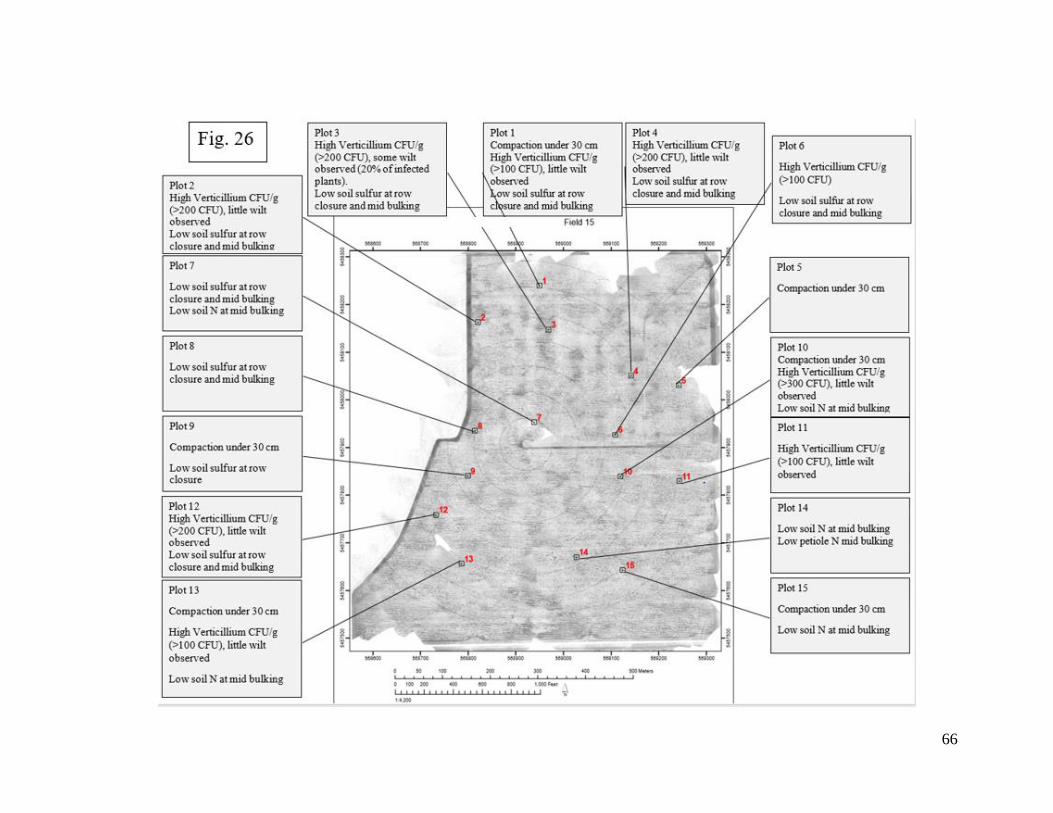
66
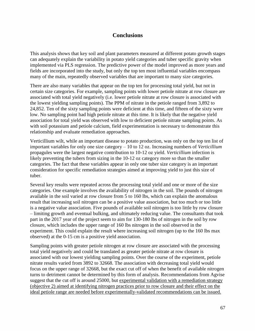
67
Conclusions
This analysis shows that key soil and plant parameters measured at different potato growth stages
can adequately explain the variability in potato yield categories and tuber specific gravity when
implemented via PLS regression. The predictive power of the model improved as more years and
fields are incorporated into the study, but only the top ten most influential variables encompass
many of the main, repeatedly observed variables that are important to many size categories.
There are also many variables that appear on the top ten for processing total yield, but not in
certain size categories. For example, sampling points with lower petiole nitrate at row closure are
associated with total yield negatively (i.e. lower petiole nitrate at row closure is associated with
the lowest yielding sampling points). The PPM of nitrate in the petiole ranged from 3,892 to
24,852. Ten of the sixty sampling points were deficient at this time, and fifteen of the sixty were
low. No sampling point had high petiole nitrate at this time. It is likely that the negative yield
association for total yield was observed with low to deficient petiole nitrate sampling points. As
with soil potassium and petiole calcium, field experimentation is necessary to demonstrate this
relationship and evaluate remediation approaches.
Verticillium wilt, while an important disease to potato production, was only on the top ten list of
important variables for only one size category – 10 to 12 oz. Increasing numbers of Verticillium
propagules were the largest negative contribution to 10-12 oz yield. Verticillium infection is
likely preventing the tubers from sizing in the 10-12 oz category more so than the smaller
categories. The fact that these variables appear in only one tuber size category is an important
consideration for specific remediation strategies aimed at improving yield to just this size of
tuber.
Several key results were repeated across the processing total yield and one or more of the size
categories. One example involves the availability of nitrogen in the soil. The pounds of nitrogen
available in the soil varied at row closure from 5 to 160 lbs, which can explain the anomalous
result that increasing soil nitrogen can be a positive value association, but too much or too little
is a negative value association. Five pounds of available soil nitrogen is too little by row closure
– limiting growth and eventual bulking, and ultimately reducing value. The consultants that took
part in the 2017 year of the project seem to aim for 130-180 lbs of nitrogen in the soil by row
closure, which includes the upper range of 160 lbs nitrogen in the soil observed in the
experiment. This could explain the result where increasing soil nitrogen (up to the 160 lbs max
observed) at the 0-15 cm is a positive yield association.
Sampling points with greater petiole nitrogen at row closure are associated with the processing
total yield negatively and could be translated as greater petiole nitrate at row closure is
associated with our lowest yielding sampling points. Over the course of the experiment, petiole
nitrate results varied from 3892 to 32668. The association with decreasing total yield would
focus on the upper range of 32668, but the exact cut off of when the benefit of available nitrogen
turns to detriment cannot be determined by this form of analysis. Recommendations from Agvise
suggest that the cut off is around 25000, but experimental validation with a remediation strategy
(objective 2) aimed at identifying nitrogen practices prior to row closure and their effect on the
ideal petiole range are needed before experimentally-validated recommendations can be issued.
68
Variables such as available sodium in the petiole are positively associated with the processing
total yield, indicating the best-yielding sampling points were associated with more petiole
sodium than the lower yielding points. The most unusual part of this observation was that petiole
sodium was often the greatest positive effect on yield or certain size categories. Over the course
of the experiment, the percentage sodium recorded in the petiole by Agvise varied from 0.01% to
0.07%, indicating the percentage range of positive benefit was small. However, the analysis
indicated that the higher percentages were associated with higher yielding sampling points. It is
also important to note that the petiole sodium content became a negative yield association from
mid bulking and late bulking, albeit not one of the top ten.
The results on petiole calcium are also interesting in that sampling points with greater petiole
calcium had lower total yield. In this case, too much or too little of calcium was associated with
lower yielding sampling points. A soil test and reference are necessary to determine whether it
was too much or too little – the model will not inform this result. The percentage of petiole
calcium at row closure ranged from 0.87-2.48%, which appeared to range from high to very
high. It is possible that excessive calcium was part of the negative yield association. As with the
nitrogen result, field experimentation is necessary to move this result from association to
concrete result that can influence recommendations.
In addition to evaluating the impact of variables on yield of all the processing fields combined,
individual fields from 2017 were rated for nutrient, soil, disease, and plant health status. Drone
imagery was used in conjunction with scouting, nutrient status as determined by Agvise
recommendations, and yield to visualize variability at each sampling point and what trends were
apparent in the overall yield. The point of this individual analysis is to demonstrate the
usefulness of the PLS analysis from all processing fields in identifying one or a few major yield-
limiting factors from a larger list of potential problems listed for a specific site. This information
begins the conversation with a local consultant and grower about priorities in remediating yield
variability, and ultimately ideal practices to remediate the situation.
Individual field analysis also highlights an interesting interaction between the June drone flight
and points of premature die down of the potato canopy. There is a possibility of using the June
flight as a predictive tool for problem places in certain fields because some spots of unhealthy
canopy already manifest by June.
On the fresh market fields, soil nitrogen and sulfur at several growth stages are associated
positively with total yield and virtually all of the size categories. Translated plainly, the higher
ranges of those nutrients were associated with our highest-yielding points. Soil nitrogen at row
closure ranged from 10.5 to 117.5 lbs N available, with more sampling points being low-to-
deficient rather than in excess of the needed nitrogen. Soil sulfur varied from 0-120 lbs available
in the soil throughout the sampling date from row closure to fall soil sampling (postharvest),
which would range from deficient to very high for ‘Russet Burbanks’. The positive yield
association points to the higher ranges (40-60 lbs were common high observations in the
experiment) as the likely yield-benefitting range, but field experimentation is needed to identify
this exact range and the best practices to get there. This is especially important given our range
of quality was determined for another cultivar other than ‘Red Norland’. The negative yield
associations for sulfur and potassium likely originate from soil samples deficient in these
nutrients.

69
There are several major limitations to these results that are necessary to keep in mind when
reading this report. Curious, interesting, or unexpected results are not necessarily biased, wrong,
or statistically inflated. These associations are based on observations across the fields included in
the experiment, and associations need a field study to further characterize the link. It is after that
characterization that scientists and consultants can try to influence that variable to full benefit on
yield. Field experimentation is especially important to address the relationship between calcium
or potassium on negative yield associations, especially before major management decisions are
implemented. Field experimentation for remediation strategies within in-field settings is a key
part of the study moving forward in order to realize these results within a potato system in an
economically feasible manner.
Most studies examining one of the factors in the experiment, such as a nutrient, analyze said
factor in isolation as part of integrity the scientific method. While this regimented, narrowed
focus is imperative for results of ideal scientific integrity, the possibility exists that several
factors are inter-related. Strategies with the intent to mitigate one factor may require additional
adjustment to other areas to achieve the desired association observed in the results of this
document. Experience has taught the author that understand the complete range of interactions of
these 97 variables is very difficult for a singular individual entity to keep in mind, yet these
interactions remain important. The route to limiting this problem is the combined, group efforts
of the research committee, as well as growers and consultants. Only in working together can the
true objective of increasing the competitiveness of Manitoba’s potato industry be realized.
70
Materials and Methods
Field Variability Study Field selection. Potato fields were deliberately chosen for exhibiting yield or quality limitations
due to soil type, topography, limited water holding capacity, compaction, or for unknown
reasons. Fields destined for French fry processing were planted with potato cultivar ‘Russet
Burbank’, and fields destined for the fresh market (that were included for analysis) were planted
to potato cultivar ‘Red Norland’. The cultivar was kept constant within the same market class to
eliminate a potential variable from analysis, and the market classes were kept separate due to
differences in cultivar growth and nutrient requirements, spatial distance between fields, as well
as the demands of each market.
Ideal fields for selection would specifically have some or all the following features: range in
variable yield and quality of previous potato crops, representative of growing conditions and
soils of potatoes in Manitoba, availability of yield maps and variability information previous to
project initiation, and grower cooperator, consultant, and processor approval of in-field
equipment use.
Having a range of yield or quality of potatoes varies within each field is important for two
reasons in order to have fields that exhibit limitations severe enough to observe repeatedly and
for the producer to consider mitigation strategies to be economically feasible. It was imperative
for fields to represent the range of conditions and practices found in Manitoba (soil types,
management practices, and environmental conditions) because the conclusions of the study need
to be applicable to the entire province, not just one growing area and crops destined for one
market. In practice, fields were selected for different soil types: sandy, clay, and silt with varying
types in-between, such as sandy-loam. Varying management practices were also taken in to
consideration, such as crop rotations, planting date, row width, irrigation type and frequency,
plant spacing, tillage practices, as well as the herbicides, fungicides, and fertilizers employed.
Encompassing Manitoba growing parameters also included environmental conditions: prevailing
weather onsite from wind speed/direction, hours of sunlight, temperature of air and soil, and
precipitation. Information and maps on previous crops in the same fields was important for
informing site selection in order to represent the maximum variability in the field. Specifically,
this included yield maps from rotational crops, other variability maps, elevation maps where
available (soils maps, soil EM maps), and aerial images from previous crops. Finally, the
growers, along with associated consultants and agronomists, are willing to consider having
treatment strips (or plots) applied in the field as well as machinery, such as quads and a tractor
with 1-row digger attached for harvest.
Sampling point selection within fields. Fifteen sampling points were established in each study
field by each May of the study year. Sampling points were determined in consultation with each
grower and their consultants using all available information: aerial imagery, variability and yield
maps, as well as producer and agronomist knowledge of the field. The sampling points will be
chosen to represent the range of field conditions and capture the areas of historical potato yield
and/or quality variability. The GPS coordinates of each sampling point would be captured by the
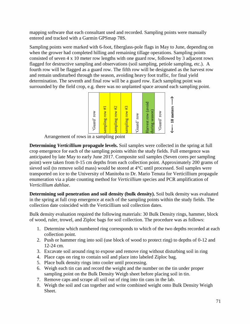
71
mapping software that each consultant used and recorded. Sampling points were manually
entered and tracked with a Garmin GPSmap 78S.
Sampling points were marked with 6-foot, fiberglass-pole flags in May to June, depending on
when the grower had completed hilling and remaining tillage operations. Sampling points
consisted of seven 4 x 10 meter row lengths with one guard row, followed by 3 adjacent rows
flagged for destructive sampling and observations (soil sampling, petiole sampling, etc.). A
fourth row will be flagged as a guard row. The fifth row will be designated as the harvest row
and remain undisturbed through the season, avoiding heavy foot traffic, for final yield
determination. The seventh and final row will be a guard row. Each sampling point was
surrounded by the field crop, e.g. there was no unplanted space around each sampling point.
‘Gu
ard
’ ro
w
sam
pli
ng
ro
w #
1
sam
pli
ng
ro
w #
2
sam
pli
ng
ro
w #
3
‘Gu
ard
’ ro
w
Har
ves
t ro
w (
avo
id
du
rin
g s
easo
n)
‘Gu
ard
’ ro
w
10
met
ers
Arrangement of rows in a sampling point
Determining Verticillium propagule levels. Soil samples were collected in the spring at full
crop emergence for each of the sampling points within the study fields. Full emergence was
anticipated by late May to early June 2017. Composite soil samples (Seven cores per sampling
point) were taken from 0-15 cm depths from each collection point. Approximately 200 grams of
sieved soil (to remove solid mass) would be stored at 4°C until processed. Soil samples were
transported on ice to the University of Manitoba to Dr. Mario Tenuta for Verticillium propagule
enumeration via a plate counting method for Verticillium species and PCR amplification of
Verticillium dahliae.
Determining soil penetration and soil density (bulk density). Soil bulk density was evaluated
in the spring at full crop emergence at each of the sampling points within the study fields. The
collection date coincided with the Verticillium soil collection dates.
Bulk density evaluation required the following materials: 30 Bulk Density rings, hammer, block
of wood, ruler, trowel, and Ziploc bags for soil collection. The procedure was as follows:
1. Determine which numbered ring corresponds to which of the two depths recorded at each
collection point.
2. Push or hammer ring into soil (use block of wood to protect ring) to depths of 0-12 and
12-24 cm.
3. Excavate soil around ring to expose and remove ring without disturbing soil in ring
4. Place caps on ring to contain soil and place into labeled Ziploc bag.
5. Place bulk density rings into cooler until processing.
6. Weigh each tin can and record the weight and the number on the tin under proper
sampling point on the Bulk Density Weigh sheet before placing soil in tin.
7. Remove caps and scrape all soil out of ring into tin cans in the lab.
8. Weigh the soil and can together and write combined weight onto Bulk Density Weigh
Sheet.
72
9. Place uncovered tins in oven at 106°C for three days.
10. Weigh the tins and soil combined again and then subtract the weight of the tin for final
dry weight and record on sheet
11. Input data from Bulk Density Weight sheet into excel spreadsheet with following
formulas:
a) Calculate volume of ring – V=πr²h b) Bulk density (g/cm3) = Dry soil weight (g)/soil volume (cm3)
c) Water content = ((wet weight – dry weight) / dry weight) * 100
Bulk density can be impacted by soil type, compaction, and tillage. Taking one bulk density
reading in a season was expected to be sufficient unless any of those three factors change after
we take our reading.
Subsurface soil compaction will be evaluated using the Manometer penetrometer available at
CMCDC at mid-bulking, which was late July in most fields. Recommended penetrometer use is
24 hours after rain, when the soil is at field capacity. Moisture must be constant for comparisons
across sites as reading can vary as soil moisture varies. A Delta-T HH2 moisture meter with
WET-2 sensor was used to determine that soil penetrometer readings are within reasonable
surface soil moisture content between sites and fields. The WET-2 sensor of the Detlta-T HH2
was used to collect 3 moisture readings from different locations within the sampling point from
depths of 4-5 cm using the following protocol (borrowed liberally from the operating manual):
1. Press Esc to wake the Moisture Meter if it is asleep.
2. Connect the sensor. The HH2 initially will assume it is an ML2 ThetaProbe in
mineral soil unless you tell it otherwise using the Options, Device menu.
3. Press Read to read and display a result.
4. Press Store to store it (or Esc to not store it).
Averaging can be done after each reading (whether or not you stored it)
5. Press the hash # key once to display the previous cumulative average.
(Initially “No Average” is displayed).
6. Press # again to update the cumulative average with the current reading (or
Esc to back out).
7. Write down the final cumulative average if you wish to retain it.
8. To erase the cumulative average press Esc until you return to “Delta-T
Devices”.
9. Output data was manually recorded on a Penetrometer Data Sheet and then data was
entered into excel sheet to calculate cone resistance with the following formula:
Cone Resistance = ((Manometer Reading)/(Base Area of Cone))/100 Mpa

73
Soil texture and water holding capacity. Composite soil samples (Seven cores per sampling
point) were taken from 0-15 cm depths from each collection point to determine % of sand, silt
and clay. In addition, a subsample will be used to determine water holding capacity. A second set
of soil samples (five cores) be collected at a depth of 15-30 cm, which will also be testing for
water holding capacity and soil texture. Samples will be collected early in the season along with
Verticillium testing and Bulk Density testing (Close to full crop emergence). Soil samples were
dried for three days after collection. Samples will be sent to Agvise for texture and water holding
capacity determination.
Soil moisture and temperature. Decagon EC50 soil data loggers with three sets of soil
moisture and temperature sensors for each logger (1 5TM 3-pronged red sensor and 2 Ec-5 2-
pronged blue sensors) have been acquired for the study to be placed in each of the 15 collection
points in two fields. The loggers were placed in June, which generally coincided with soil
sampling and bulk density.
Cellular EM50G Decagon logger and sensor protocol
Materials:
• Sensors (3/logger)
a) One 5TM sensor
b) Two EC-5 sensors
• Decagon Logger
• Tall Stake
• Auger
• Ruler
• Flags
• Zip ties (2/logger)
• Batteries (5/logger)
• Desiccant Pack
• Antenna
• Computer and USB cord to connect manually to logger
• Burlap sack
Preparation:
• Go to http://www.ech2o.com/accounts/login/?next=/ and enter each unique Device ID
and password that comes with each individual EM50G logger. Also add this information
into DataTrac3 to get live feeds of data being collected.
• Connect every EM50G logger to Ech2o Utility or DataTrac3 program to configure
EM50G logger. Set measurement interval to one hour on each logger, under Device
Identity and Name, enter logger name that is on the front of the logger. Under Data
Storage and Port Sensor 1, 2, 3, choose which sensors you are using. Under Device
Location and Site Name, enter the point at which the logger is being installed.
• Preform communication test by connecting logger with antenna attached to Ech2o or
DataTrac3 program and clicking on “Actions” pull down menu and then selecting
“Communications Test,” then click “Test.” If the logger does not have a good connection
quality, try moving to a different location or outside of the building, or change the
74
batteries. You can also select “List Cellular Carries” under the “Actions” pull down menu
to see if the logger is picking up any signal from any cellular carrier.
• Label each sensor at the non-probe end corresponding to which port it will be inserted in
to. The 5TM sensor (3-pronged red sensor) should be labelled “1” and the two EC-5 (2-
pronged blue sensors) should be labelled “2” and the other “3.” If the sensor cables are of
different lengths, reserve the longer one for the deeper depth. On the inside of the logger,
there will be a paper slip in the sleeve called “Em50 Port Configuration.” On this sheet,
indicate which depths the sensors will be installed at. “1” should be the 5TM sensor
installed at depth of 6 cm, “2” is the EC-5 sensor installed at 15 cm, “3” the last EC-5
sensor installed at 30 cm.
Installation:
1. Dig a hole in the hill with the auger to desired depth (30 cm). As you dig, place the soil
onto the burlap sack so that each horizon can approximately be placed back in the same
order after completion of sensor installation.
2. Place the ruler on the flat edge of the hole made by the auger and make pilot holes with a
pin flag at depths of 6 cm, 15 cm, and 30 cm. Then, insert the prongs of the sensors from
the bottom depth up into the pilot holes with the EC-5 sensor labelled “3” at 30 cm, the
EC-5 sensor labelled “2” at 15 cm, and the 5TM sensor labelled “1” at 6 cm. Make sure
that the prongs have sufficient soil contact for an accurate reading, later in season,
potatoes may grow and dislodge the prongs or may grow into the prongs themselves and
give an inaccurate moisture reading that is too high. If this happens, re-installation of the
affected sensors will be required.
3. Unravel the appropriate amount of chord needed for the sensor to reach to the logger at
the top of the stake (make sure the stake is tall enough so that the antenna on the logger
will be above the canopy for a good cellular signal). Group the male input ends of the
cable together, so that once the hole is filled, all wires will come up out of the ground at
the same site. Bundle the unneeded amount of cable back up with the twist tie and then
bury the cables with soil that was laid to the side on the burlap sack. Attempt to replace
the soil back at the correct horizons.
4. Attach the logger to the top of the stake with the two provided zip ties. Insert the batteries
and the male input into the correct ports labelled “1,” “2,” and “3.” Attach the antenna to
the top of the logger, place desiccant pack inside and close the logger.
5. Manually connect the logger to the laptop with the USB chord and open Ech2o utility.
Once connected, select scan to ensure that the sensors were installed correctly and are
producing moisture readings.
6. Mark the location of the wires with pin flags and ensure that the stake is marked with
bright colour so that it is clearly visible to field workers.
Soil nutrient evaluation. Soil and Petiole samples were collected at row closure, mid bulking,
and late bulking to determine in-season nutrient availability. Soils were collected from each of
the 15 sampling points in each field, and each point had be previously marked out with flags that
were not removed between sampling dates, implying that GPS confirmation of location was not
necessary between collection dates. Row closure was anticipated in early July, mid bulking in
late July, and late bulking in late August. Soils were sampled five times with a probe at 0-15 cm
and 15-30 cm, and composite soil samples from both depths at each sampling point were tested

75
through Agvise for NO3, P-Olsen, K, and S. Soils were kept at 4⁰C between field sampling and
shipment for testing.
Soil samples will also be collected in the fall following crop harvest, which is anticipated to be
complete by October. Flags denoting sampling points were removed before harvest, necessitating
the following protocol for fall soil sampling:
Procedure:
1. Use GPS to re-locate points after harvest
2. Samples from two depths will be taken, 0-15 cm and 15-60 cm. Take three full length
cores (0-60 cm) with the hydraulic-probe and take an additional three 0-15 cm cores with
the hand-probe.
3. Twist both bags for each depth together and tie. Store for processing later
4. Lay soil out in chem shed or Bernie’s shed on butcher paper, place labelled field soil
collection bag underneath butcher paper with corresponding sample ontop
5. Allow soil to dry for three days
6. Sieve soil and place into labelled Agvise bags and place into Agvise box along with
proper spreadsheet containing the information of each sampling point
7. Ship to Portage
Analysis by Agvise was completed for fall soil samples. Specifically, nitrogen (2 depths),
phosphorus, potassium, pH, soluble salts, sulfur, zinc, calcium, magnesium, sodium, CEC, and
percentage organic matter were evaluated.
Plant assessment. Plant counts will be collected on the 10-meter row lengths of the harvest row
for each study point after crop emergence, but before row closure.
Counts on sampling row lengths are collected to determine the number of plants being assessed
at later visits. Comparable numbers of plants between sampling points is important when
comparing factors such as yield, which can be influenced by the number of plants. Plant counts
therefore served as a quality control check for the initial health of the stand and crop before that
collection point is used for continued experimentation.
Plant disease assessments. Field visits assessed crop growth and health following emergence at
each sampling point in each field. Field visits varied in frequency from once a week to once
every two weeks. The notes from these visits were to be used with data and imagery
interpretation at a later date. If crop issues arise during the growing season within study fields,
regular visits and notes may point to additional sampling or data collection. Field notes to be
taken included: crop growth stage, visual crop stress symptoms, visual crop disease symptoms,
and crop pests and weeds notes.
The only consistent disease rating across two years of study (2016-17) was aVerticillium rating,
in which one of the established 10 m sampling rows was chosen to evaluate vascular
discoloration in potato stems and wilt symptoms for the whole plant using published disease
charts (below). These charts were provided by Dr. Vikram Bisht. In 2017, direct estimation of
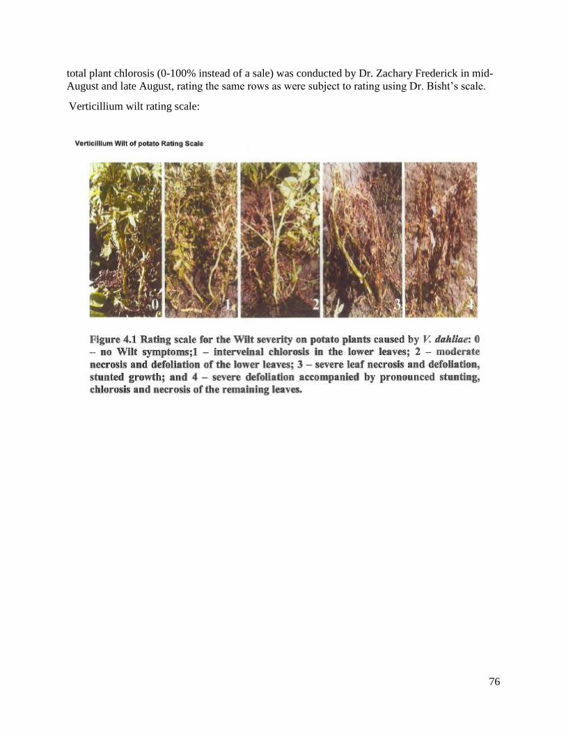
76
total plant chlorosis (0-100% instead of a sale) was conducted by Dr. Zachary Frederick in mid-
August and late August, rating the same rows as were subject to rating using Dr. Bisht’s scale.
Verticillium wilt rating scale:
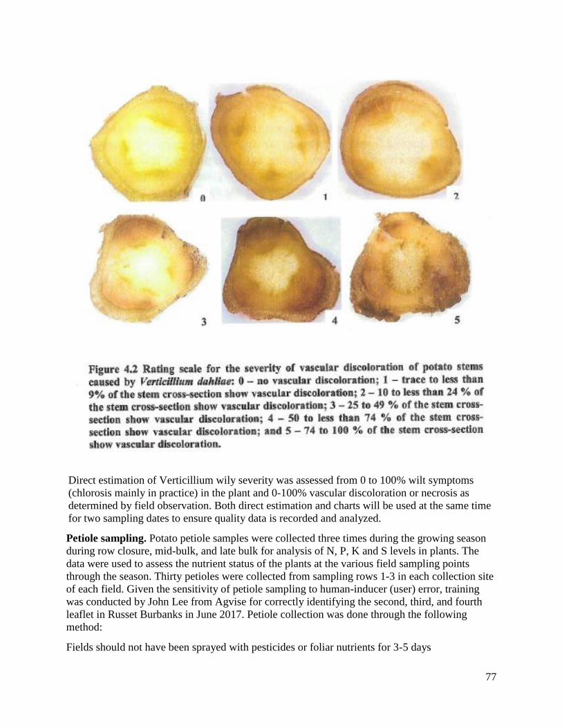
77
Direct estimation of Verticillium wily severity was assessed from 0 to 100% wilt symptoms
(chlorosis mainly in practice) in the plant and 0-100% vascular discoloration or necrosis as
determined by field observation. Both direct estimation and charts will be used at the same time
for two sampling dates to ensure quality data is recorded and analyzed.
Petiole sampling. Potato petiole samples were collected three times during the growing season
during row closure, mid-bulk, and late bulk for analysis of N, P, K and S levels in plants. The
data were used to assess the nutrient status of the plants at the various field sampling points
through the season. Thirty petioles were collected from sampling rows 1-3 in each collection site
of each field. Given the sensitivity of petiole sampling to human-inducer (user) error, training
was conducted by John Lee from Agvise for correctly identifying the second, third, and fourth
leaflet in Russet Burbanks in June 2017. Petiole collection was done through the following
method:
Fields should not have been sprayed with pesticides or foliar nutrients for 3-5 days
78
• Sample from all 15 sites, use rows 1 and 2 and 3, 30 petioles per site, go in zig zag
down the rows.
• Select plants without an inflorescence if possible.
• Attempt to maintain similar sizes of petiole throughout sample, attempt to maintain
petiole length of a minimum of three inches after stripping leaves
• Do no include snapped, torn, crushed, or otherwise damaged petioles
• Select 4th petiole from the top of the meristem, samples should not come in contact
with dirt.
• Samples must be maintained in as cool temperatures as possible and not be exposed
to sunlight.
• Samples should be delivered for processing immediately.
Tuber yield and quality. The selected 10m harvest row will be harvested in Late August or
September, and will be ahead of the producer’s harvest but be as close as possible. Total harvest
weight and quality grading will be done separately on each of the 15 samples taken from the
study fields, and based on crop sector (fresh or processing). Processing yield and quality will be
determined by Agworld at the McCain Foods (Canada) plant in Carberry. Fresh market field
yield and quality will be determined by a consultant, Kurt Ginter, in Winkler.
Weather data. Weather information from available weather stations near to the fields were used
to better understand the interactions between the factors associated to field variability and the
crop performance. Mean temperature, daily minimums and maximums, relative humidity, rain
events and wind will be recorded in an excel spreadsheet. One field in each year of study will
also have a Hobo weather station temporarily installed onsite, with sensors for Mean
temperature, daily minimums and maximums, relative humidity, rain events, solar radiation, and
wind.
Drone Imagery. Drone images will be collected from the beginning of the season on bare soil to
capture elevation, moisture and any other observable variability factors within the field. Drone
images will also be collected three times throughout the season: At row closure, late bulking, and
at senescence.
NIR and true color images will be collected at each of the three in-crop image dates. Four
ground-control points be established in each 2017 processing field (4 fields total) prior to the
collection of the drone imagery to assist with proper geo-referencing of the images. Ther fixed-
wing drone used a parrot sequoia camera that records green, red, red edge, near IR. It has a 70
degree field of view and catches one image per second that was stitched together using ArcGIS.
We get about 13 cm per pixel at 120m. The 15 collection points per field were identified in 2017
based on GPS coordinates recorded on the ground, the average Normalized Difference
Vegetation Index (NDVI) value for the collection point was extracted into a table using ArcGIS
and Microsoft Excel. These tables were then used for statistical analysis in SAS and graphical
display in Microsoft Excel.
Statistical Analysis with the Partial Least Squares Regression method The relationships between potato yield and quality parameters as dependent variables and 97
independent variables were explored with Partial Least Squares regression analysis with the
primary goal to identify the key ten to twenty variables explaining the yield and quality
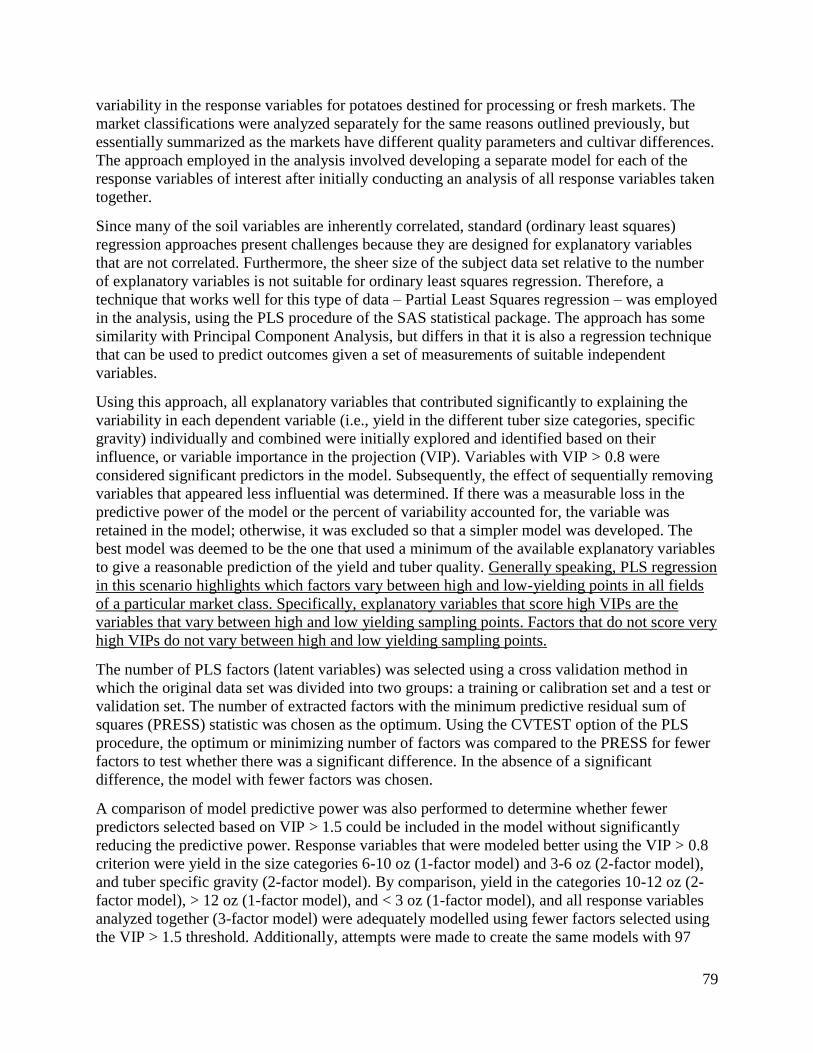
79
variability in the response variables for potatoes destined for processing or fresh markets. The
market classifications were analyzed separately for the same reasons outlined previously, but
essentially summarized as the markets have different quality parameters and cultivar differences.
The approach employed in the analysis involved developing a separate model for each of the
response variables of interest after initially conducting an analysis of all response variables taken
together.
Since many of the soil variables are inherently correlated, standard (ordinary least squares)
regression approaches present challenges because they are designed for explanatory variables
that are not correlated. Furthermore, the sheer size of the subject data set relative to the number
of explanatory variables is not suitable for ordinary least squares regression. Therefore, a
technique that works well for this type of data – Partial Least Squares regression – was employed
in the analysis, using the PLS procedure of the SAS statistical package. The approach has some
similarity with Principal Component Analysis, but differs in that it is also a regression technique
that can be used to predict outcomes given a set of measurements of suitable independent
variables.
Using this approach, all explanatory variables that contributed significantly to explaining the
variability in each dependent variable (i.e., yield in the different tuber size categories, specific
gravity) individually and combined were initially explored and identified based on their
influence, or variable importance in the projection (VIP). Variables with VIP > 0.8 were
considered significant predictors in the model. Subsequently, the effect of sequentially removing
variables that appeared less influential was determined. If there was a measurable loss in the
predictive power of the model or the percent of variability accounted for, the variable was
retained in the model; otherwise, it was excluded so that a simpler model was developed. The
best model was deemed to be the one that used a minimum of the available explanatory variables
to give a reasonable prediction of the yield and tuber quality. Generally speaking, PLS regression
in this scenario highlights which factors vary between high and low-yielding points in all fields
of a particular market class. Specifically, explanatory variables that score high VIPs are the
variables that vary between high and low yielding sampling points. Factors that do not score very
high VIPs do not vary between high and low yielding sampling points.
The number of PLS factors (latent variables) was selected using a cross validation method in
which the original data set was divided into two groups: a training or calibration set and a test or
validation set. The number of extracted factors with the minimum predictive residual sum of
squares (PRESS) statistic was chosen as the optimum. Using the CVTEST option of the PLS
procedure, the optimum or minimizing number of factors was compared to the PRESS for fewer
factors to test whether there was a significant difference. In the absence of a significant
difference, the model with fewer factors was chosen.
A comparison of model predictive power was also performed to determine whether fewer
predictors selected based on VIP > 1.5 could be included in the model without significantly
reducing the predictive power. Response variables that were modeled better using the VIP > 0.8
criterion were yield in the size categories 6-10 oz (1-factor model) and 3-6 oz (2-factor model),
and tuber specific gravity (2-factor model). By comparison, yield in the categories 10-12 oz (2-
factor model), > 12 oz (1-factor model), and < 3 oz (1-factor model), and all response variables
analyzed together (3-factor model) were adequately modelled using fewer factors selected using
the VIP > 1.5 threshold. Additionally, attempts were made to create the same models with 97

80
dependent variables and 10, 20, or 30 of the most influential dependent variables. Decreasing the
number of dependant variables decreased predictive power and the quality of the resulting
model, therefore all 97 dependant variables were used. The top 10 dependant variables could still
be reported, but it is important to consider that the model requires as many inputs from
dependant variables as possible to achieve the “best” predictive model (best defined as the model
greatest predictive power, least scatter).
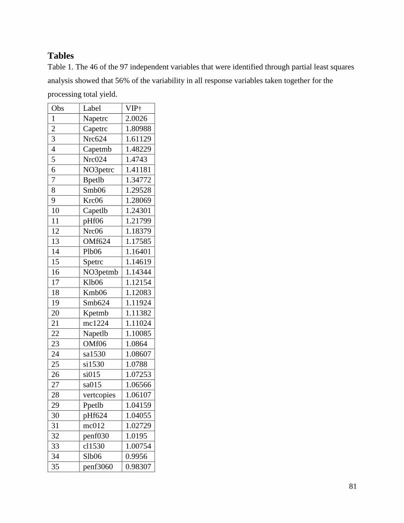
81
Tables
Table 1. The 46 of the 97 independent variables that were identified through partial least squares
analysis showed that 56% of the variability in all response variables taken together for the
processing total yield.
Obs Label VIP†
1 Napetrc 2.0026
2 Capetrc 1.80988
3 Nrc624 1.61129
4 Capetmb 1.48229
5 Nrc024 1.4743
6 NO3petrc 1.41181
7 Bpetlb 1.34772
8 Smb06 1.29528
9 Krc06 1.28069
10 Capetlb 1.24301
11 pHf06 1.21799
12 Nrc06 1.18379
13 OMf624 1.17585
14 Plb06 1.16401
15 Spetrc 1.14619
16 NO3petmb 1.14344
17 Klb06 1.12154
18 Kmb06 1.12083
19 Smb624 1.11924
20 Kpetmb 1.11382
21 mc1224 1.11024
22 Napetlb 1.10085
23 OMf06 1.0864
24 sa1530 1.08607
25 si1530 1.0788
26 si015 1.07253
27 sa015 1.06566
28 vertcopies 1.06107
29 Ppetlb 1.04159
30 pHf624 1.04055
31 mc012 1.02729
32 penf030 1.0195
33 cl1530 1.00754
34 Slb06 0.9956
35 penf3060 0.98307
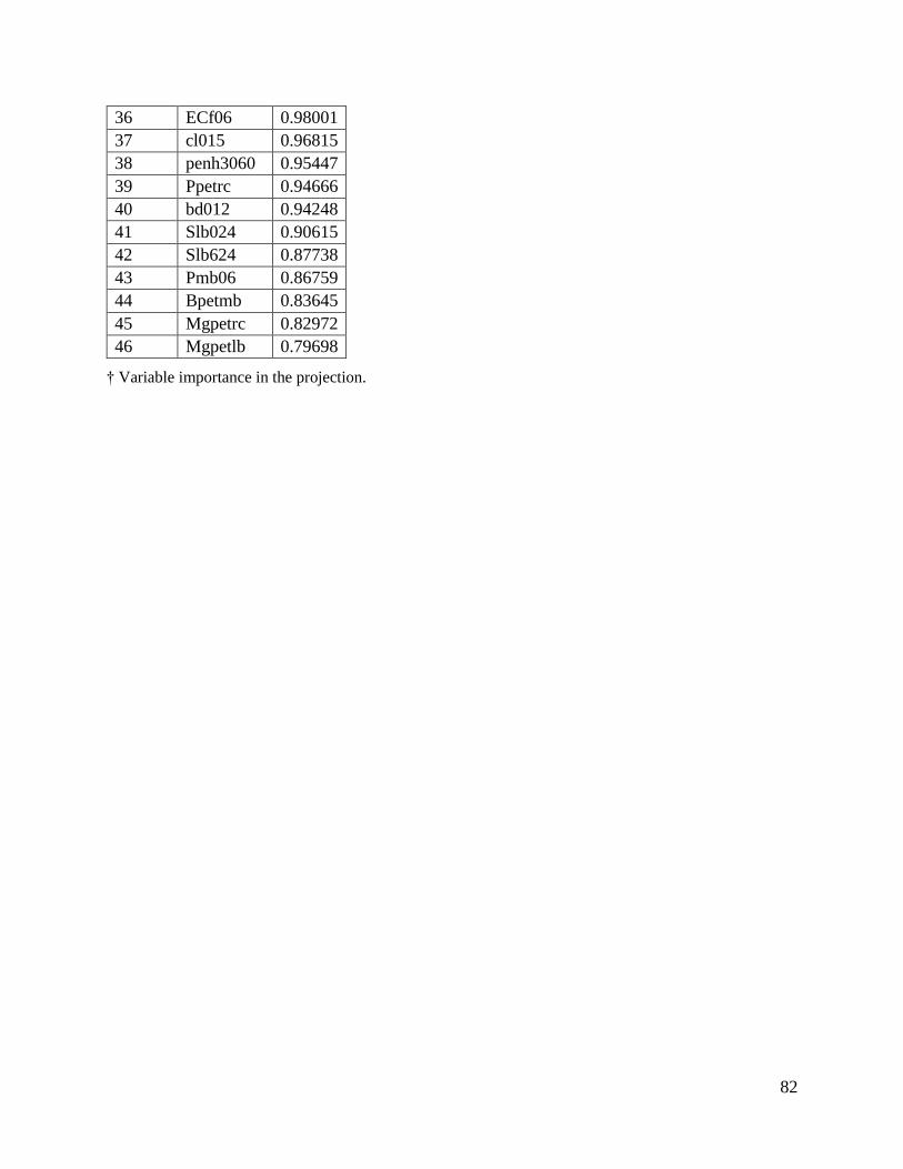
82
36 ECf06 0.98001
37 cl015 0.96815
38 penh3060 0.95447
39 Ppetrc 0.94666
40 bd012 0.94248
41 Slb024 0.90615
42 Slb624 0.87738
43 Pmb06 0.86759
44 Bpetmb 0.83645
45 Mgpetrc 0.82972
46 Mgpetlb 0.79698
† Variable importance in the projection.

83
Table 2. The 46 of the 97 independent variables that were identified through partial least squares
analysis showed that 58% of the variability in all response variables taken together for the
processing value.
Obs Label VIP †
1 Napetrc 2.11621
2 Capetrc 1.93348
3 Nrc624 1.55998
4 Nrc024 1.50282
5 Capetmb 1.48782
6 Smb06 1.42632
7 Capetlb 1.31038
8 Nrc06 1.29746
9 Napetlb 1.28349
10 Krc06 1.26368
11 NO3petrc 1.2524
12 Bpetlb 1.17175
13 Plb06 1.16575
14 OMf624 1.1594
15 vertcopies 1.13335
16 Kpetmb 1.13124
17 Spetrc 1.1191
18 ECf06 1.11586
19 mc1224 1.10633
20 NO3petmb 1.09028
21 si1530 1.08177
22 penf030 1.07939
23 OMf06 1.07078
24 Klb06 1.07038
25 sa1530 1.0693
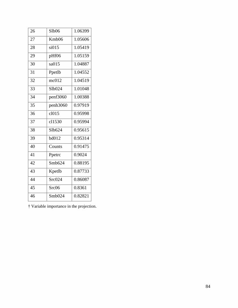
84
26 Slb06 1.06399
27 Kmb06 1.05606
28 si015 1.05419
29 pHf06 1.05159
30 sa015 1.04887
31 Ppetlb 1.04552
32 mc012 1.04519
33 Slb024 1.01048
34 penf3060 1.00388
35 penh3060 0.97919
36 cl015 0.95998
37 cl1530 0.95994
38 Slb624 0.95615
39 bd012 0.95314
40 Counts 0.91475
41 Ppetrc 0.9024
42 Smb624 0.88195
43 Kpetlb 0.87733
44 Src024 0.86087
45 Src06 0.8361
46 Smb024 0.82821
† Variable importance in the projection.
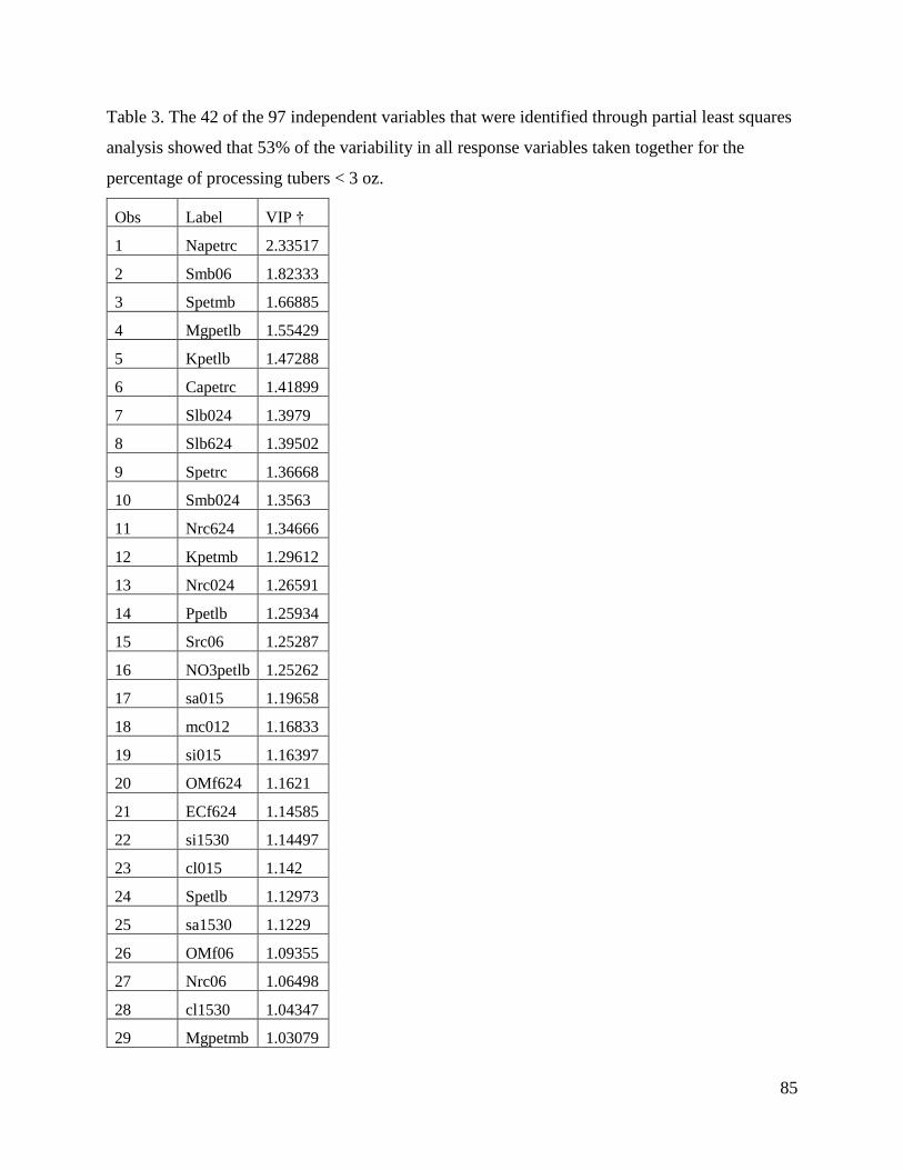
85
Table 3. The 42 of the 97 independent variables that were identified through partial least squares
analysis showed that 53% of the variability in all response variables taken together for the
percentage of processing tubers < 3 oz.
Obs Label VIP †
1 Napetrc 2.33517
2 Smb06 1.82333
3 Spetmb 1.66885
4 Mgpetlb 1.55429
5 Kpetlb 1.47288
6 Capetrc 1.41899
7 Slb024 1.3979
8 Slb624 1.39502
9 Spetrc 1.36668
10 Smb024 1.3563
11 Nrc624 1.34666
12 Kpetmb 1.29612
13 Nrc024 1.26591
14 Ppetlb 1.25934
15 Src06 1.25287
16 NO3petlb 1.25262
17 sa015 1.19658
18 mc012 1.16833
19 si015 1.16397
20 OMf624 1.1621
21 ECf624 1.14585
22 si1530 1.14497
23 cl015 1.142
24 Spetlb 1.12973
25 sa1530 1.1229
26 OMf06 1.09355
27 Nrc06 1.06498
28 cl1530 1.04347
29 Mgpetmb 1.03079
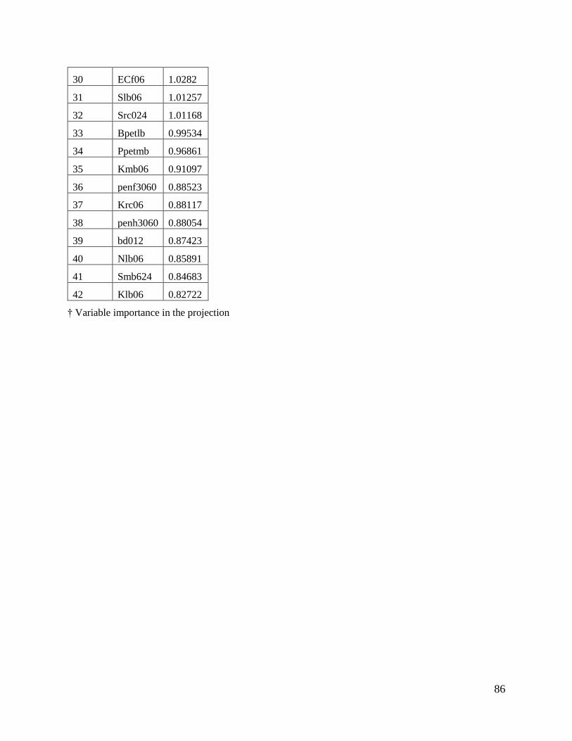
86
30 ECf06 1.0282
31 Slb06 1.01257
32 Src024 1.01168
33 Bpetlb 0.99534
34 Ppetmb 0.96861
35 Kmb06 0.91097
36 penf3060 0.88523
37 Krc06 0.88117
38 penh3060 0.88054
39 bd012 0.87423
40 Nlb06 0.85891
41 Smb624 0.84683
42 Klb06 0.82722
† Variable importance in the projection
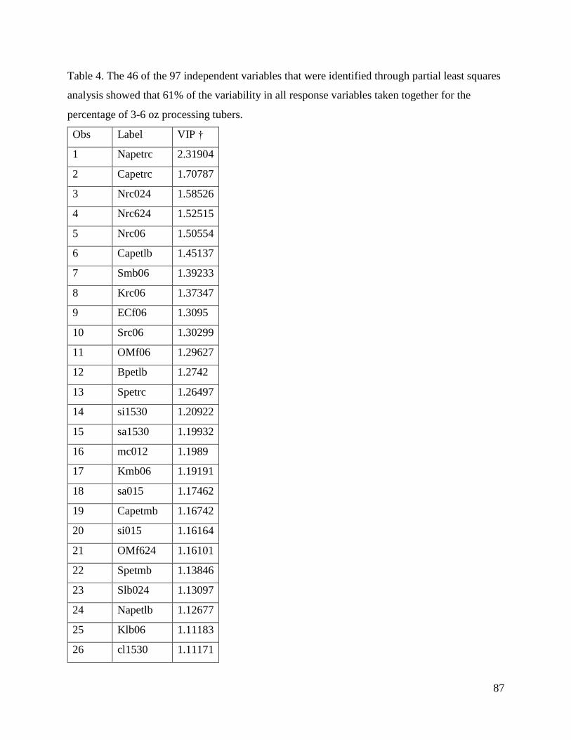
87
Table 4. The 46 of the 97 independent variables that were identified through partial least squares
analysis showed that 61% of the variability in all response variables taken together for the
percentage of 3-6 oz processing tubers.
Obs Label VIP †
1 Napetrc 2.31904
2 Capetrc 1.70787
3 Nrc024 1.58526
4 Nrc624 1.52515
5 Nrc06 1.50554
6 Capetlb 1.45137
7 Smb06 1.39233
8 Krc06 1.37347
9 ECf06 1.3095
10 Src06 1.30299
11 OMf06 1.29627
12 Bpetlb 1.2742
13 Spetrc 1.26497
14 si1530 1.20922
15 sa1530 1.19932
16 mc012 1.1989
17 Kmb06 1.19191
18 sa015 1.17462
19 Capetmb 1.16742
20 si015 1.16164
21 OMf624 1.16101
22 Spetmb 1.13846
23 Slb024 1.13097
24 Napetlb 1.12677
25 Klb06 1.11183
26 cl1530 1.11171
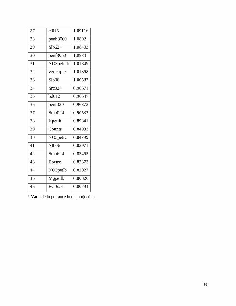
88
27 cl015 1.09116
28 penh3060 1.0892
29 Slb624 1.08403
30 penf3060 1.0834
31 NO3petmb 1.01849
32 vertcopies 1.01358
33 Slb06 1.00587
34 Src024 0.96671
35 bd012 0.96547
36 penf030 0.96373
37 Smb024 0.90537
38 Kpetlb 0.89841
39 Counts 0.84933
40 NO3petrc 0.84799
41 Nlb06 0.83971
42 Smb624 0.83455
43 Bpetrc 0.82373
44 NO3petlb 0.82027
45 Mgpetlb 0.80826
46 ECf624 0.80794
† Variable importance in the projection.
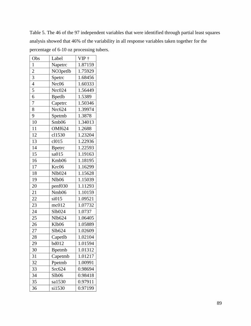
89
Table 5. The 46 of the 97 independent variables that were identified through partial least squares
analysis showed that 46% of the variability in all response variables taken together for the
percentage of 6-10 oz processing tubers.
Obs Label VIP †
1 Napetrc 1.87159
2 NO3petlb 1.75929
3 Spetrc 1.68456
4 Nrc06 1.60333
5 Nrc024 1.56449
6 Bpetlb 1.5389
7 Capetrc 1.50346
8 Nrc624 1.39974
9 Spetmb 1.3878
10 Smb06 1.34013
11 OMf624 1.2688
12 cl1530 1.23204
13 cl015 1.22936
14 Bpetrc 1.22593
15 sa015 1.19163
16 Kmb06 1.18195
17 Krc06 1.16299
18 Nlb024 1.15628
19 Nlb06 1.15039
20 penf030 1.11293
21 Nmb06 1.10159
22 si015 1.09521
23 mc012 1.07732
24 Slb024 1.0737
25 Nlb624 1.06405
26 Klb06 1.05889
27 Slb624 1.02609
28 Capetlb 1.02104
29 bd012 1.01594
30 Bpetmb 1.01312
31 Capetmb 1.01217
32 Ppetmb 1.00991
33 Src624 0.98694
34 Slb06 0.98418
35 sa1530 0.97911
36 si1530 0.97199
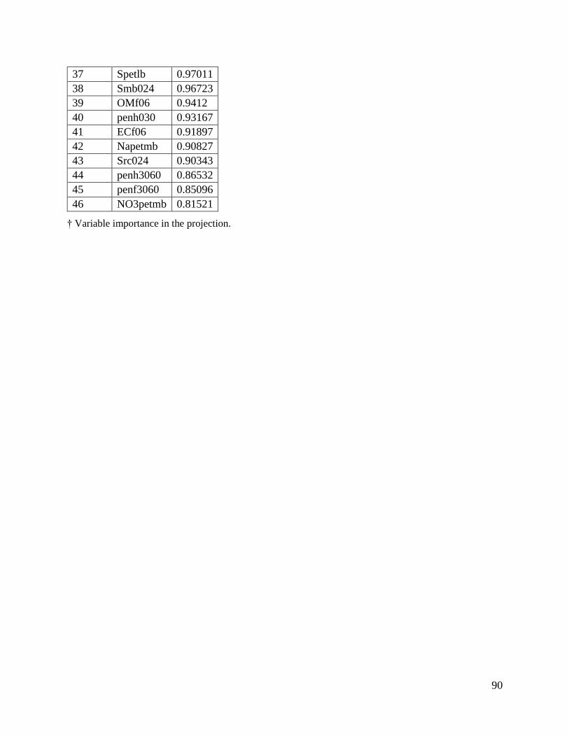
90
37 Spetlb 0.97011
38 Smb024 0.96723
39 OMf06 0.9412
40 penh030 0.93167
41 ECf06 0.91897
42 Napetmb 0.90827
43 Src024 0.90343
44 penh3060 0.86532
45 penf3060 0.85096
46 NO3petmb 0.81521
† Variable importance in the projection.
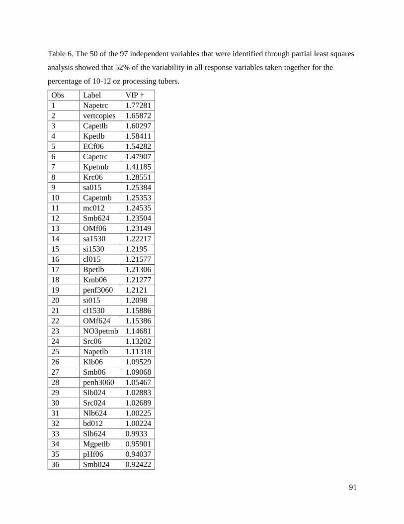
91
Table 6. The 50 of the 97 independent variables that were identified through partial least squares
analysis showed that 52% of the variability in all response variables taken together for the
percentage of 10-12 oz processing tubers.
Obs Label VIP †
1 Napetrc 1.77281
2 vertcopies 1.65872
3 Capetlb 1.60297
4 Kpetlb 1.58411
5 ECf06 1.54282
6 Capetrc 1.47907
7 Kpetmb 1.41185
8 Krc06 1.28551
9 sa015 1.25384
10 Capetmb 1.25353
11 mc012 1.24535
12 Smb624 1.23504
13 OMf06 1.23149
14 sa1530 1.22217
15 si1530 1.2195
16 cl015 1.21577
17 Bpetlb 1.21306
18 Kmb06 1.21277
19 penf3060 1.2121
20 si015 1.2098
21 cl1530 1.15886
22 OMf624 1.15386
23 NO3petmb 1.14681
24 Src06 1.13202
25 Napetlb 1.11318
26 Klb06 1.09529
27 Smb06 1.09068
28 penh3060 1.05467
29 Slb024 1.02883
30 Src024 1.02689
31 Nlb624 1.00225
32 bd012 1.00224
33 Slb624 0.9933
34 Mgpetlb 0.95901
35 pHf06 0.94037
36 Smb024 0.92422
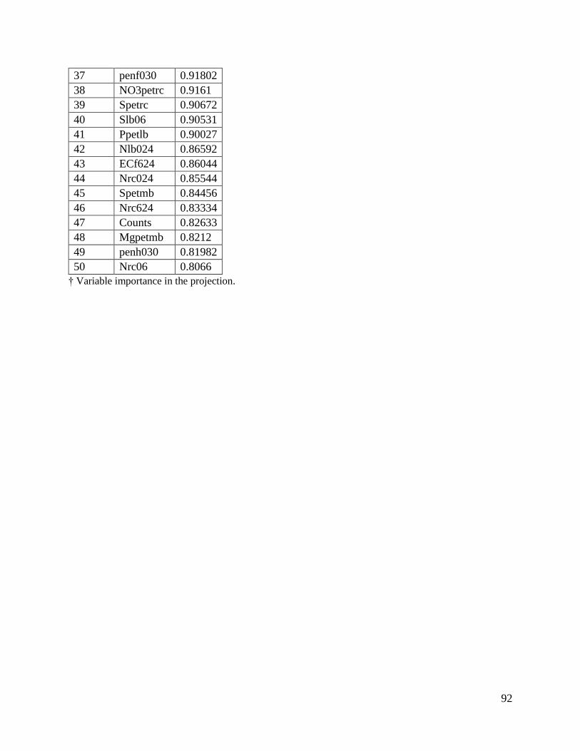
92
37 penf030 0.91802
38 NO3petrc 0.9161
39 Spetrc 0.90672
40 Slb06 0.90531
41 Ppetlb 0.90027
42 Nlb024 0.86592
43 ECf624 0.86044
44 Nrc024 0.85544
45 Spetmb 0.84456
46 Nrc624 0.83334
47 Counts 0.82633
48 Mgpetmb 0.8212
49 penh030 0.81982
50 Nrc06 0.8066
† Variable importance in the projection.
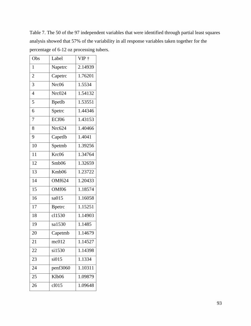
93
Table 7. The 50 of the 97 independent variables that were identified through partial least squares
analysis showed that 57% of the variability in all response variables taken together for the
percentage of 6-12 oz processing tubers.
Obs Label VIP †
1 Napetrc 2.14939
2 Capetrc 1.76201
3 Nrc06 1.5534
4 Nrc024 1.54132
5 Bpetlb 1.53551
6 Spetrc 1.44346
7 ECf06 1.43153
8 Nrc624 1.40466
9 Capetlb 1.4041
10 Spetmb 1.39256
11 Krc06 1.34764
12 Smb06 1.32659
13 Kmb06 1.23722
14 OMf624 1.20433
15 OMf06 1.18574
16 sa015 1.16058
17 Bpetrc 1.15251
18 cl1530 1.14903
19 sa1530 1.1485
20 Capetmb 1.14679
21 mc012 1.14527
22 si1530 1.14398
23 si015 1.1334
24 penf3060 1.10311
25 Klb06 1.09879
26 cl015 1.09648
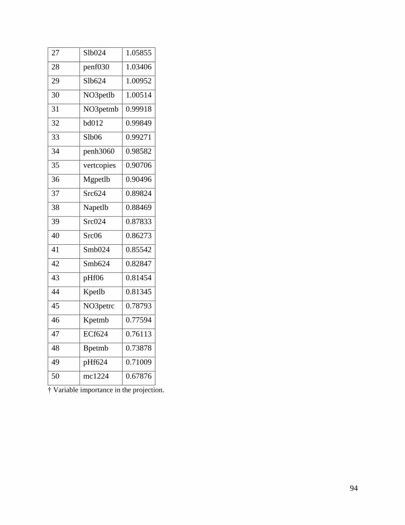
94
27 Slb024 1.05855
28 penf030 1.03406
29 Slb624 1.00952
30 NO3petlb 1.00514
31 NO3petmb 0.99918
32 bd012 0.99849
33 Slb06 0.99271
34 penh3060 0.98582
35 vertcopies 0.90706
36 Mgpetlb 0.90496
37 Src624 0.89824
38 Napetlb 0.88469
39 Src024 0.87833
40 Src06 0.86273
41 Smb024 0.85542
42 Smb624 0.82847
43 pHf06 0.81454
44 Kpetlb 0.81345
45 NO3petrc 0.78793
46 Kpetmb 0.77594
47 ECf624 0.76113
48 Bpetmb 0.73878
49 pHf624 0.71009
50 mc1224 0.67876
† Variable importance in the projection.
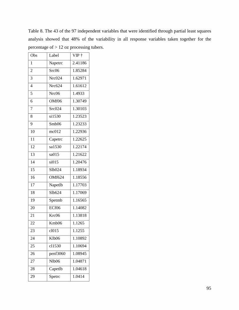
95
Table 8. The 43 of the 97 independent variables that were identified through partial least squares
analysis showed that 48% of the variability in all response variables taken together for the
percentage of > 12 oz processing tubers.
Obs Label VIP †
1 Napetrc 2.41186
2 Src06 1.85284
3 Nrc024 1.62971
4 Nrc624 1.61612
5 Nrc06 1.4933
6 OMf06 1.30749
7 Src024 1.30103
8 si1530 1.23523
9 Smb06 1.23233
10 mc012 1.22936
11 Capetrc 1.22625
12 sa1530 1.22174
13 sa015 1.21622
14 si015 1.20476
15 Slb024 1.18934
16 OMf624 1.18556
17 Napetlb 1.17703
18 Slb624 1.17069
19 Spetmb 1.16565
20 ECf06 1.14082
21 Krc06 1.13818
22 Kmb06 1.1265
23 cl015 1.1255
24 Klb06 1.10892
25 cl1530 1.10694
26 penf3060 1.08945
27 Nlb06 1.04871
28 Capetlb 1.04618
29 Spetrc 1.0414
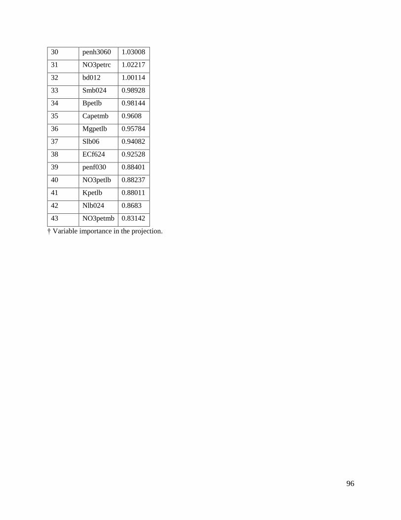
96
30 penh3060 1.03008
31 NO3petrc 1.02217
32 bd012 1.00114
33 Smb024 0.98928
34 Bpetlb 0.98144
35 Capetmb 0.9608
36 Mgpetlb 0.95784
37 Slb06 0.94082
38 ECf624 0.92528
39 penf030 0.88401
40 NO3petlb 0.88237
41 Kpetlb 0.88011
42 Nlb024 0.8683
43 NO3petmb 0.83142
† Variable importance in the projection.
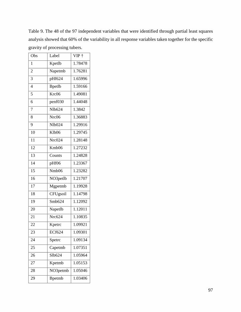
97
Table 9. The 48 of the 97 independent variables that were identified through partial least squares
analysis showed that 60% of the variability in all response variables taken together for the specific
gravity of processing tubers.
Obs Label VIP †
1 Kpetlb 1.78478
2 Napetmb 1.76281
3 pHf624 1.65996
4 Bpetlb 1.59166
5 Krc06 1.49081
6 penf030 1.44048
7 Nlb624 1.3842
8 Nrc06 1.36883
9 Nlb024 1.29916
10 Klb06 1.29745
11 Nrc024 1.28148
12 Kmb06 1.27232
13 Counts 1.24828
14 pHf06 1.23367
15 Nmb06 1.23282
16 NO3petlb 1.21707
17 Mgpetmb 1.19928
18 CFUgsoil 1.14798
19 Smb624 1.12092
20 Napetlb 1.12011
21 Nrc624 1.10835
22 Kpetrc 1.09921
23 ECf624 1.09301
24 Spetrc 1.09134
25 Capetmb 1.07351
26 Slb624 1.05964
27 Kpetmb 1.05153
28 NO3petmb 1.05046
29 Bpetmb 1.03406
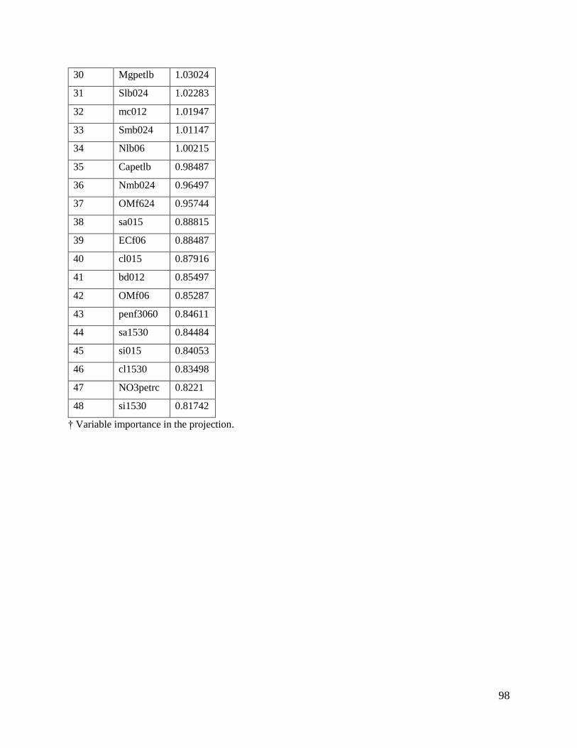
98
30 Mgpetlb 1.03024
31 Slb024 1.02283
32 mc012 1.01947
33 Smb024 1.01147
34 Nlb06 1.00215
35 Capetlb 0.98487
36 Nmb024 0.96497
37 OMf624 0.95744
38 sa015 0.88815
39 ECf06 0.88487
40 cl015 0.87916
41 bd012 0.85497
42 OMf06 0.85287
43 penf3060 0.84611
44 sa1530 0.84484
45 si015 0.84053
46 cl1530 0.83498
47 NO3petrc 0.8221
48 si1530 0.81742
† Variable importance in the projection.
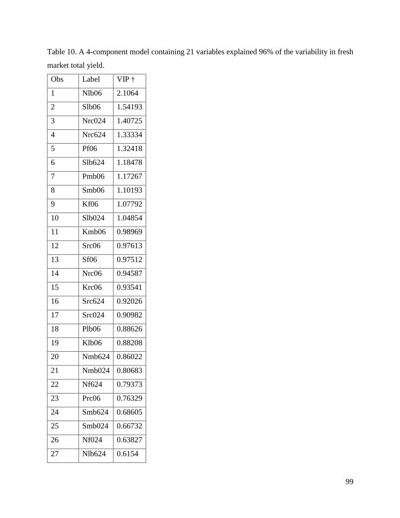
99
Table 10. A 4-component model containing 21 variables explained 96% of the variability in fresh
market total yield.
Obs Label VIP †
1 Nlb06 2.1064
2 Slb06 1.54193
3 Nrc024 1.40725
4 Nrc624 1.33334
5 Pf06 1.32418
6 Slb624 1.18478
7 Pmb06 1.17267
8 Smb06 1.10193
9 Kf06 1.07792
10 Slb024 1.04854
11 Kmb06 0.98969
12 Src06 0.97613
13 Sf06 0.97512
14 Nrc06 0.94587
15 Krc06 0.93541
16 Src624 0.92026
17 Src024 0.90982
18 Plb06 0.88626
19 Klb06 0.88208
20 Nmb624 0.86022
21 Nmb024 0.80683
22 Nf624 0.79373
23 Prc06 0.76329
24 Smb624 0.68605
25 Smb024 0.66732
26 Nf024 0.63827
27 Nlb624 0.6154
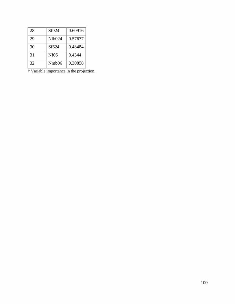
100
28 Sf024 0.60916
29 Nlb024 0.57677
30 Sf624 0.48484
31 Nf06 0.4344
32 Nmb06 0.30858
† Variable importance in the projection.
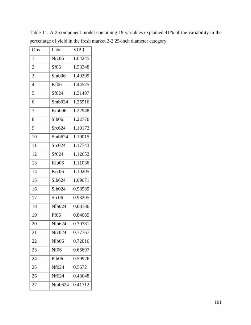
101
Table 11. A 2-component model containing 19 variables explained 41% of the variability in the
percentage of yield in the fresh market 2-2.25-inch diameter category.
Obs Label VIP †
1 Nrc06 1.64245
2 Sf06 1.53348
3 Smb06 1.49209
4 Kf06 1.44525
5 Sf024 1.31407
6 Smb024 1.25916
7 Kmb06 1.22948
8 Slb06 1.22776
9 Src624 1.19172
10 Smb624 1.19015
11 Src024 1.17743
12 Sf624 1.12652
13 Klb06 1.11036
14 Krc06 1.10205
15 Slb624 1.09071
16 Slb024 0.98989
17 Src06 0.98205
18 Nlb024 0.88786
19 Pf06 0.84085
20 Nlb624 0.79781
21 Nrc024 0.77767
22 Nlb06 0.72016
23 Nf06 0.66697
24 Plb06 0.59926
25 Nf024 0.5672
26 Nf624 0.48648
27 Nmb624 0.41712
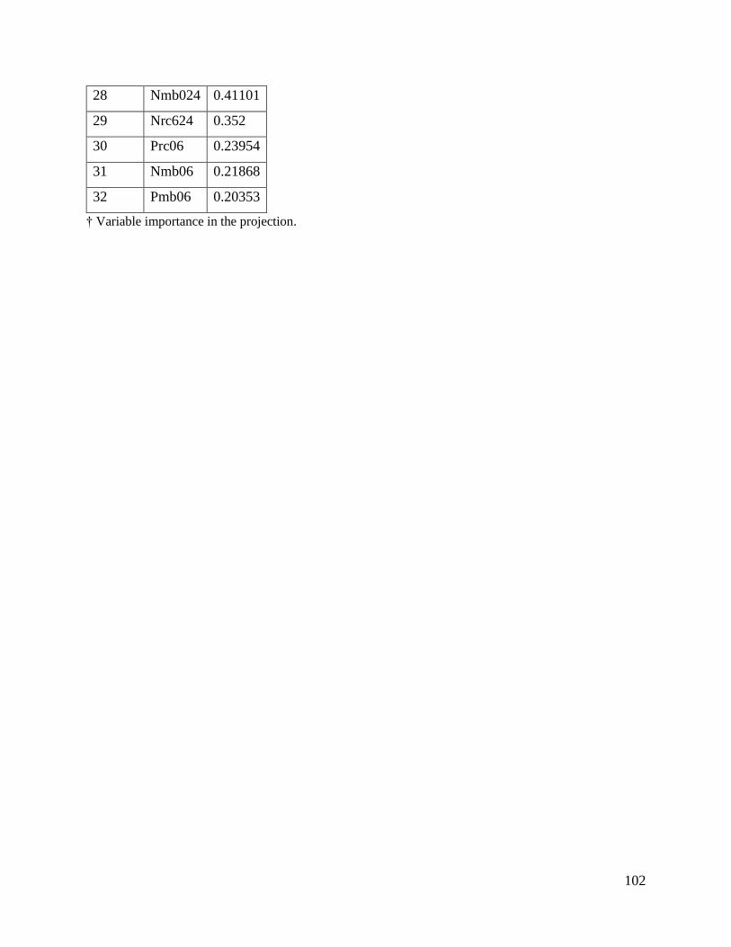
102
28 Nmb024 0.41101
29 Nrc624 0.352
30 Prc06 0.23954
31 Nmb06 0.21868
32 Pmb06 0.20353
† Variable importance in the projection.

103
Table 12. A 2-component model containing 17 variables explained 52% of the variability in the
percentage of yield in the fresh market 2.25 to 3.0-inch diameter category.
Obs Label VIP †
1 Smb06 1.86031
2 Nrc06 1.65166
3 Smb024 1.41118
4 Sf06 1.37166
5 Kf06 1.30696
6 Sf024 1.28875
7 Smb624 1.28632
8 Src624 1.26438
9 Kmb06 1.25066
10 Src024 1.23864
11 Klb06 1.19088
12 Sf624 1.19055
13 Krc06 1.11581
14 Slb624 1.10322
15 Slb024 1.04242
16 Src06 0.93008
17 Nf06 0.91616
18 Nrc024 0.77504
19 Nf024 0.74318
20 Slb06 0.737
21 Pf06 0.63511
22 Nf624 0.55272
23 Nmb024 0.52433
24 Nmb624 0.50932
25 Pmb06 0.49097
26 Prc06 0.47319
27 Nlb624 0.44465
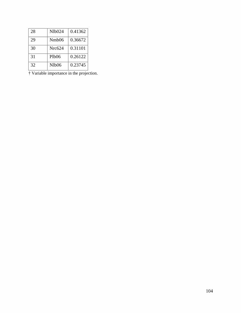
104
28 Nlb024 0.41362
29 Nmb06 0.36672
30 Nrc624 0.31101
31 Plb06 0.26122
32 Nlb06 0.23745
† Variable importance in the projection.
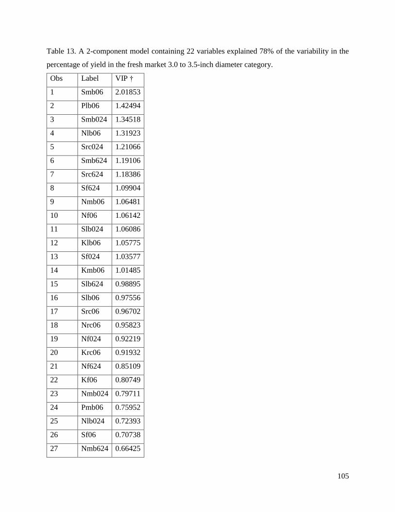
105
Table 13. A 2-component model containing 22 variables explained 78% of the variability in the
percentage of yield in the fresh market 3.0 to 3.5-inch diameter category.
Obs Label VIP †
1 Smb06 2.01853
2 Plb06 1.42494
3 Smb024 1.34518
4 Nlb06 1.31923
5 Src024 1.21066
6 Smb624 1.19106
7 Src624 1.18386
8 Sf624 1.09904
9 Nmb06 1.06481
10 Nf06 1.06142
11 Slb024 1.06086
12 Klb06 1.05775
13 Sf024 1.03577
14 Kmb06 1.01485
15 Slb624 0.98895
16 Slb06 0.97556
17 Src06 0.96702
18 Nrc06 0.95823
19 Nf024 0.92219
20 Krc06 0.91932
21 Nf624 0.85109
22 Kf06 0.80749
23 Nmb024 0.79711
24 Pmb06 0.75952
25 Nlb024 0.72393
26 Sf06 0.70738
27 Nmb624 0.66425
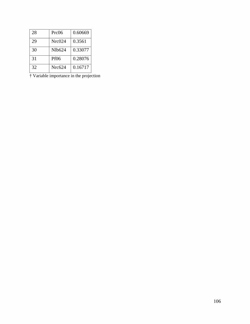
106
28 Prc06 0.60669
29 Nrc024 0.3561
30 Nlb624 0.33077
31 Pf06 0.28076
32 Nrc624 0.16717
† Variable importance in the projection